


1 Introduction
The study of moduli spaces is a central topic in algebraic geometry; among moduli spaces, Hilbert schemes form an important class of examples. They have been widely studied in geometric representation theory, enumerative and combinatorial geometry and as two of the only four known deformation classes of hyperkähler manifolds, namely Hilbert schemes of points on K3 surfaces and generalised Kummer varieties. A prominent direction in this area is to understand the local moduli space of such objects and, in particular, methods for describing modular simple normal crossing degenerations of smooth Hilbert schemes. We study how the technique of expanded degenerations applies to this problem for Hilbert schemes of points on surfaces.
1.1 Main results
Expanded degenerations are first introduced by Li [Reference Li10] and then used by Li and Wu [Reference Li and Wu11] to study Quot schemes on degenerations $\pi \colon X\to \mathbb A^1$
such that
$\pi \colon X\to \mathbb A^1$
such that $(X,\pi ^{-1}(0))$
is a simple normal crossing pair, where the singular locus of
$(X,\pi ^{-1}(0))$
is a simple normal crossing pair, where the singular locus of $\pi ^{-1}(0)$
is smooth. This paper explores the connection between two ideas:
$\pi ^{-1}(0)$
is smooth. This paper explores the connection between two ideas:
-
1. The logarithmic geometry approach to this problem considered by Maulik and Ranganathan in [Reference Maulik and Ranganathan12].
-
2. The Geometric Invariant Theory (GIT) perspective of Gulbrandsen, Halle and Hulek [Reference Gulbrandsen, Halle and Hulek6].
The construction presented in this paper is the first instance of a logarithmic moduli space of coherent sheaves built using ideas from GIT. As, historically, GIT has been used to consider stability of objects, we hope that this work can provide insights into describing stability for logarithmic sheaves. As mentioned in Section 1.3, our constructions also give minimal models for type III degenerations of Hilbert schemes of points on K3 surfaces. This is described in our paper [Reference Tschanz21].
We construct two equivalent modular simple normal crossing degenerations of smooth Hilbert schemes of points on surfaces. These extend [Reference Li and Wu11] and [Reference Gulbrandsen, Halle and Hulek6] to the case where the singular locus of $\pi ^{-1}(0)$
is singular. Understanding how these problems work in general for simple normal crossings is quite powerful, as we can always use semistable reduction to reduce to this case.
$\pi ^{-1}(0)$
is singular. Understanding how these problems work in general for simple normal crossings is quite powerful, as we can always use semistable reduction to reduce to this case.
The first degeneration of Hilbert schemes of points we construct is a stack $\mathfrak {M}^m_{\operatorname {\mathrm {LW}}}$
which uses a generalisation of Li-Wu stability to this situation (see Definition 5.3.2). The second is a stack
$\mathfrak {M}^m_{\operatorname {\mathrm {LW}}}$
which uses a generalisation of Li-Wu stability to this situation (see Definition 5.3.2). The second is a stack $\mathfrak {M}^m_{\operatorname {\mathrm {SWS}}}$
which uses a stability condition called SWS stability (see Definition 5.3.5) derived from GIT. This provides an explicit model of the degenerations theorised in [Reference Maulik and Ranganathan12] and we describe how these can be interpreted in the language of logarithmic geometry. The main results of this paper are the following.
$\mathfrak {M}^m_{\operatorname {\mathrm {SWS}}}$
which uses a stability condition called SWS stability (see Definition 5.3.5) derived from GIT. This provides an explicit model of the degenerations theorised in [Reference Maulik and Ranganathan12] and we describe how these can be interpreted in the language of logarithmic geometry. The main results of this paper are the following.
Theorem 1.1.1. The stacks $\mathfrak {M}^m_{\operatorname {\mathrm {LW}}}$
and
$\mathfrak {M}^m_{\operatorname {\mathrm {LW}}}$
and $\mathfrak {M}^m_{\operatorname {\mathrm {SWS}}}$
are Deligne-Mumford and proper over C.
$\mathfrak {M}^m_{\operatorname {\mathrm {SWS}}}$
are Deligne-Mumford and proper over C.
Theorem 1.1.2. There is an isomorphism of stacks
 $$\begin{align*}\mathfrak{M}^m_{\operatorname{\mathrm{LW}}}\cong \mathfrak{M}^m_{\operatorname{\mathrm{SWS}}}. \end{align*}$$
These stacks are also semistable degenerations over C. This is shown in [Reference Shafi and Tschanz19].
1.2 Setup and key ideas
Let k be an algebraically closed field of characteristic zero. Let $X\to C$
be a flat projective family of surfaces over a curve
$X\to C$
be a flat projective family of surfaces over a curve $C\cong \mathbb A^1$
. We take this family to be semistable, i.e. its total space is smooth and its central fibre
$C\cong \mathbb A^1$
. We take this family to be semistable, i.e. its total space is smooth and its central fibre $X_0$
is simple normal crossing. At a triple point of the singular fibre, X is étale locally given by
$X_0$
is simple normal crossing. At a triple point of the singular fibre, X is étale locally given by $\operatorname {\mathrm {Spec}} k[x,y,z,t]/(xyz-t)$
. In this étale local model, the general fibres are smooth and the central fibre
$\operatorname {\mathrm {Spec}} k[x,y,z,t]/(xyz-t)$
. In this étale local model, the general fibres are smooth and the central fibre $X_0$
is given by three planes intersecting transversely in
$X_0$
is given by three planes intersecting transversely in $\mathbb A^3$
. Throughout this work, these will be denoted
$\mathbb A^3$
. Throughout this work, these will be denoted $Y_1,Y_2$
and
$Y_1,Y_2$
and $Y_3$
, given in local coordinates by
$Y_3$
, given in local coordinates by $x=0,\ y=0$
and
$x=0,\ y=0$
and $z=0$
respectively.
$z=0$
respectively.
We may consider the relative Hilbert scheme of m points over $X\to C$
, denoted
$X\to C$
, denoted $\operatorname {\mathrm {Hilb}}^m(X/C)$
. The special fibre
$\operatorname {\mathrm {Hilb}}^m(X/C)$
. The special fibre $\operatorname {\mathrm {Hilb}}^m(X_0)$
of this degeneration is very singular. Our aim is to propose a different model of this degeneration, where the special fibre is simple normal crossing. This may be rephrased as the following compactification problem. Let
$\operatorname {\mathrm {Hilb}}^m(X_0)$
of this degeneration is very singular. Our aim is to propose a different model of this degeneration, where the special fibre is simple normal crossing. This may be rephrased as the following compactification problem. Let ![]() , which lies over
, which lies over ![]() . We may then look for compactifications of the relative Hilbert scheme of m points
. We may then look for compactifications of the relative Hilbert scheme of m points $\operatorname {\mathrm {Hilb}}^m(X^\circ /C^\circ )$
, which satisfy the desired properties.
$\operatorname {\mathrm {Hilb}}^m(X^\circ /C^\circ )$
, which satisfy the desired properties.
We say a zero dimensional closed subscheme of $X_0$
is smoothly supported if its support is contained within the smooth locus of
$X_0$
is smoothly supported if its support is contained within the smooth locus of $X_0$
. The locus of zero dimensional closed subschemes satisfying this property is not proper. The problem therefore is to modify
$X_0$
. The locus of zero dimensional closed subschemes satisfying this property is not proper. The problem therefore is to modify $X_0$
by constructing expansions (see Definition 2.1.2, in this case they will be birational modifications of X in
$X_0$
by constructing expansions (see Definition 2.1.2, in this case they will be birational modifications of X in $X_0$
) in which the limits of families of length m zero-dimensional subschemes needed to compactify
$X_0$
) in which the limits of families of length m zero-dimensional subschemes needed to compactify $\operatorname {\mathrm {Hilb}}^m(X^\circ /C^\circ )$
can be chosen to be smoothly supported. This allows us to break down the problem of studying Hilbert schemes of points on
$\operatorname {\mathrm {Hilb}}^m(X^\circ /C^\circ )$
can be chosen to be smoothly supported. This allows us to break down the problem of studying Hilbert schemes of points on $X_0$
into smaller parts, by studying the products of Hilbert schemes of points on the irreducible components of the modifications of X. See [Reference Maulik and Ranganathan13] for applications of this type of construction to enumerative geometry.
$X_0$
into smaller parts, by studying the products of Hilbert schemes of points on the irreducible components of the modifications of X. See [Reference Maulik and Ranganathan13] for applications of this type of construction to enumerative geometry.
1.3 Further results
This construction has the benefit of being very straightforward compared to the other possible constructions solving this problem, as we will discuss later. The restrictive choices made in the construction of the universal family of expansions $\mathfrak {X}$
mean that LW or SWS stability are already sufficient conditions to make the stacks of stable objects proper. This is unexpected and shows that the example we construct here is very special among all possible models of such good compactifications; indeed, in general we will need to take an additional stability condition, as can be seen in [Reference Maulik and Ranganathan12] (see Section 2.2 for the role of Donaldson-Thomas stability in this problem). In [Reference Tschanz21], we discuss how this additional stability condition can be expressed in the language we set up here.
$\mathfrak {X}$
mean that LW or SWS stability are already sufficient conditions to make the stacks of stable objects proper. This is unexpected and shows that the example we construct here is very special among all possible models of such good compactifications; indeed, in general we will need to take an additional stability condition, as can be seen in [Reference Maulik and Ranganathan12] (see Section 2.2 for the role of Donaldson-Thomas stability in this problem). In [Reference Tschanz21], we discuss how this additional stability condition can be expressed in the language we set up here.
Allowing for different choices of expansions.
In [Reference Tschanz21], we build upon these results to describe other choices of models. In this second paper, we consider an approach which parallels work of Kennedy-Hunt on logarithmic Quot schemes [Reference Kennedy-Hunt8], as well as recover certain geometrically meaningful choices of moduli stacks arising from the methods of Maulik and Ranganathan [Reference Maulik and Ranganathan12]. In particular, we discuss how tube components and Donaldson-Thomas stability enter the picture in these more general cases (see Section 2.2 for definitions), by defining an analogue of this stability condition for our constructions. Another explicit choice of expansions arises in the work of Mok [Reference Chi Mok14] on Logarithmic Fulton-MacPherson configuration spaces. The choice of expansion of Mok is more symmetric but results in a singular degeneration.
Application to hyperkähler varieties.
We only consider here the property that $\pi \colon X\to C$
is a degeneration of surfaces where
$\pi \colon X\to C$
is a degeneration of surfaces where $(X,X_0)$
is a simple normal crossing pair. A natural question is to study the more specific case where X is a type III good degeneration of K3 surfaces and try to construct a family of Hilbert schemes of points on X which will be minimal in the sense of the minimal model program, meaning a good or dlt minimal degeneration (see [Reference Nagai16] and [Reference Kollár, Laza, Saccà and Voisin9] for definitions of minimality conditions). This was done by the author and Shafi in [Reference Shafi and Tschanz19]. The singularities arising in such a degeneration X are of the type described here, i.e. we can restrict ourselves to the local problem where
$(X,X_0)$
is a simple normal crossing pair. A natural question is to study the more specific case where X is a type III good degeneration of K3 surfaces and try to construct a family of Hilbert schemes of points on X which will be minimal in the sense of the minimal model program, meaning a good or dlt minimal degeneration (see [Reference Nagai16] and [Reference Kollár, Laza, Saccà and Voisin9] for definitions of minimality conditions). This was done by the author and Shafi in [Reference Shafi and Tschanz19]. The singularities arising in such a degeneration X are of the type described here, i.e. we can restrict ourselves to the local problem where $X_0$
is thought of as given by
$X_0$
is thought of as given by $xyz=0$
in
$xyz=0$
in $\mathbb A^3$
. Among other reasons, Hilbert schemes of points on K3 surfaces are interesting to study because they form a class of examples of hyperkähler varieties. The question of minimality is addressed in [Reference Tschanz21].
$\mathbb A^3$
. Among other reasons, Hilbert schemes of points on K3 surfaces are interesting to study because they form a class of examples of hyperkähler varieties. The question of minimality is addressed in [Reference Tschanz21].
1.4 Organisation
We start, in Section 2, by giving some background on logarithmic and tropical geometry, and an overview of the work of Maulik and Ranganathan from [Reference Maulik and Ranganathan12] which we will want to refer to in later sections. Then, in Section 3, we set out an expanded construction on schemes and, in 4, we discuss how various GIT stability conditions can be defined on this construction. In Section 5, we describe a corresponding stack of expansions and family over it, building on the expanded degenerations we constructed as schemes. In Section 6, we extend our stability conditions to this setting. We then show that the stacks of stable objects defined have the desired Deligne-Mumford and properness properties.
2 Background on tropical perspective
We briefly introduce here the language of tropical and logarithmic geometry in the context of this problem. For more details on the contents of this section, see the article [Reference Abramovich, Chen, Gillam, Huang, Olsson, Satriano and Sun1], lecture notes [Reference Ranganathan17], as well as the first section of [Reference Maulik and Ranganathan12].
2.1 Tropicalisation and expansion
Tropicalisation.
Let $(X,\mathcal M_X)$
be a logarithmic scheme, where the sheaf of monoids
$(X,\mathcal M_X)$
be a logarithmic scheme, where the sheaf of monoids $\mathcal M_X$
gives the divisorial logarithmic structure with respect to some simple normal crossing divisor
$\mathcal M_X$
gives the divisorial logarithmic structure with respect to some simple normal crossing divisor $D\subset X$
. Explicitly, for an open subset
$D\subset X$
. Explicitly, for an open subset $U \subseteq X$
, the sheaf
$U \subseteq X$
, the sheaf $\mathcal M_X$
is given by
$\mathcal M_X$
is given by
Then we can associate a fan $\Sigma _X$
to this in the following way. Recall that the characteristic sheaf
$\Sigma _X$
to this in the following way. Recall that the characteristic sheaf $\overline {\mathcal M}_X$
for the divisorial logarithmic structure is defined by
$\overline {\mathcal M}_X$
for the divisorial logarithmic structure is defined by
 $$\begin{align*}\overline{\mathcal M}_X = \mathcal M_{X}/\mathcal O_X^*. \end{align*}$$
The sheaf $\mathcal M_{X}$
records functions vanishing at most on D and
$\mathcal M_{X}$
records functions vanishing at most on D and $\overline {\mathcal M}_X$
records their vanishing orders. For each point
$\overline {\mathcal M}_X$
records their vanishing orders. For each point $x\in X$
, there is an isomorphism
$x\in X$
, there is an isomorphism $\overline {\mathcal M}_{X,x} \cong \mathbb N^k$
, where k is the number of components of D which contain x. We let
$\overline {\mathcal M}_{X,x} \cong \mathbb N^k$
, where k is the number of components of D which contain x. We let
This will be contained in $\mathbb R^r_{\geq 0}$
, where r is the number of components of D, since D is a simple normal crossing divisor. We call
$\mathbb R^r_{\geq 0}$
, where r is the number of components of D, since D is a simple normal crossing divisor. We call $\Sigma _X$
the tropicalisation of X.
$\Sigma _X$
the tropicalisation of X.
Subdivisions of the tropicalisation define expansions of X.
In the following, we will want to study possible monomial birational modifications of the scheme X around the divisor D. In the tropical language, these are expressed as subdivisions.
Definition 2.1.1. Let $\Upsilon $
be a fan, let
$\Upsilon $
be a fan, let $|\Upsilon |$
be its support and
$|\Upsilon |$
be its support and $\upsilon $
be a continuous map
$\upsilon $
be a continuous map
 $$\begin{align*}\upsilon\colon |\Upsilon| \longrightarrow \Sigma_X \end{align*}$$
such that the image of every cone in $\Upsilon $
is contained in a cone of
$\Upsilon $
is contained in a cone of $\Sigma _X$
and that is given by an integral linear map when restricted to each cone in
$\Sigma _X$
and that is given by an integral linear map when restricted to each cone in $\Upsilon $
. We say that
$\Upsilon $
. We say that $\upsilon $
is a subdivision if it is injective on the support of
$\upsilon $
is a subdivision if it is injective on the support of $\Upsilon $
and the integral points of the image of each cone
$\Upsilon $
and the integral points of the image of each cone $\tau \in \Upsilon $
are exactly the intersection of the integral points of
$\tau \in \Upsilon $
are exactly the intersection of the integral points of $\Sigma _X$
with
$\Sigma _X$
with $\tau $
.
$\tau $
.
A subdivision of the tropicalisation defines a birational modification of X in the following way (for a reference on toric geometry, see [Reference Fulton5]). The subdivision
has an associated toric variety $\mathbb A_{\Upsilon }$
, which comes with a
$\mathbb A_{\Upsilon }$
, which comes with a $\mathbb G^r_m$
-equivariant birational map
$\mathbb G^r_m$
-equivariant birational map $\mathbb A_\Upsilon \to \mathbb A^r$
. Then we have an induced morphism of quotient stacks
$\mathbb A_\Upsilon \to \mathbb A^r$
. Then we have an induced morphism of quotient stacks
 $$\begin{align*}[\mathbb A_\Upsilon/\mathbb G_m^r] \longrightarrow [\mathbb A^r/\mathbb G_m^r] \end{align*}$$
and we may define the induced birational modification of X to be
Definition 2.1.2. We say that the birational modification described above is an expansion of X.
Visualising the problem.
Here, we describe how to visualise the tropicalisation arising from the divisorial logarithmic structure on X associated to a simple normal crossing divisor $D\subset X$
. We explain this for the case which interests us here, that is, we assume that
$D\subset X$
. We explain this for the case which interests us here, that is, we assume that $X\to C$
is locally given by
$X\to C$
is locally given by $\operatorname {\mathrm {Spec}} k[x,y,z,t]/(xyz-t)$
and the boundary divisor is
$\operatorname {\mathrm {Spec}} k[x,y,z,t]/(xyz-t)$
and the boundary divisor is ![]() .
.
Given a divisorial logarithmic structure on X, the tropicalisation is a fan or cone complex which for each defining function of the divisor records the degree of vanishing of this function in X. Here, the functions vanishing at D will be $x,y$
and z. As
$x,y$
and z. As $X_0$
is made up of three components meeting in a point, in this case we may actually represent
$X_0$
is made up of three components meeting in a point, in this case we may actually represent $\Sigma _X$
as a fan in
$\Sigma _X$
as a fan in $\mathbb R^3_{\geq 0}$
, given by the positive orthant and its faces, as can be seen in Figure 1. In this image the three half-lines correspond to the divisors
$\mathbb R^3_{\geq 0}$
, given by the positive orthant and its faces, as can be seen in Figure 1. In this image the three half-lines correspond to the divisors $Y_1,\ Y_2$
and
$Y_1,\ Y_2$
and $Y_3$
in X. We may think of these half-lines as recording the orders of vanishing in
$Y_3$
in X. We may think of these half-lines as recording the orders of vanishing in $x,y$
and z respectively. The 2-dimensional faces spanned by two half-lines correspond to the orders of vanishing in both coordinates vanishing at
$x,y$
and z respectively. The 2-dimensional faces spanned by two half-lines correspond to the orders of vanishing in both coordinates vanishing at $Y_i\cap Y_j$
, and the three-dimensional interior of the cone corresponds to the triple intersection point
$Y_i\cap Y_j$
, and the three-dimensional interior of the cone corresponds to the triple intersection point $Y_1\cap Y_2\cap Y_3$
, i.e. records orders of vanishing in all three variables. For convenience, we shall refer to this tropicalisation as
$Y_1\cap Y_2\cap Y_3$
, i.e. records orders of vanishing in all three variables. For convenience, we shall refer to this tropicalisation as $\operatorname {\mathrm {trop}}(X)$
in later sections.
$\operatorname {\mathrm {trop}}(X)$
in later sections.

Figure 1 Tropicalisation of X.
The dual complex of $X_0$
(see [Reference de Fernex, Kollár and Xu4] for a definition) can be visualised by taking a hyperplane slice through the cone in Figure 1; this yields a triangle with vertices corresponding to
$X_0$
(see [Reference de Fernex, Kollár and Xu4] for a definition) can be visualised by taking a hyperplane slice through the cone in Figure 1; this yields a triangle with vertices corresponding to $Y_1,Y_2$
and
$Y_1,Y_2$
and $Y_3$
in
$Y_3$
in $X_0$
, edges between these vertices corresponding to the lines
$X_0$
, edges between these vertices corresponding to the lines $Y_i\cap Y_j$
, and 2-dimensional interior corresponding to the point
$Y_i\cap Y_j$
, and 2-dimensional interior corresponding to the point $Y_1\cap Y_2\cap Y_3$
, as pictured in Figure 2. We shall abuse notation and refer to the dual complex of
$Y_1\cap Y_2\cap Y_3$
, as pictured in Figure 2. We shall abuse notation and refer to the dual complex of $X_0$
as
$X_0$
as $\operatorname {\mathrm {trop}}(X_0)$
.
$\operatorname {\mathrm {trop}}(X_0)$
.

Figure 2 Tropicalisation of $X_0$
.
$X_0$
.
Recall that $C\cong \mathbb A^1$
and it can be considered to be a logarithmic scheme with divisorial logarithmic structure given by
$C\cong \mathbb A^1$
and it can be considered to be a logarithmic scheme with divisorial logarithmic structure given by $0\in C$
. The fan of
$0\in C$
. The fan of $\mathbb A^1$
is a half-line with a distinguished vertex. The map
$\mathbb A^1$
is a half-line with a distinguished vertex. The map $X\to C$
can be seen as a log smooth morphism of log schemes and, in this case, tropicalisation is functorial. Making a choice of point on this half-line therefore corresponds to choosing a height for the triangle within the cone
$X\to C$
can be seen as a log smooth morphism of log schemes and, in this case, tropicalisation is functorial. Making a choice of point on this half-line therefore corresponds to choosing a height for the triangle within the cone $\mathbb R^3_{\geq 0}$
. Geometrically, we can think of changing the height of the triangle as making a finite base change on X.
$\mathbb R^3_{\geq 0}$
. Geometrically, we can think of changing the height of the triangle as making a finite base change on X.
2.2 Maulik-Ranganathan construction
We will briefly recall some key points of [Reference Maulik and Ranganathan12]. The aim of their work is to study the moduli space of ideal sheaves of fixed numerical type which meet the boundary divisor transversely and satisfy some predeformability condition (see [Reference Ranganathan18]). The space of ideal sheaves satisfying these properties is noncompact and the theory of expansions is used to construct a space which is proper over C. In the case of Hilbert schemes of points, it will also be flat over C, although in general this is not true. In [Reference Maulik and Ranganathan12], Maulik and Ranganathan construct appropriate compactifications and formulate the Donaldson-Thomas theory of the pair $(X,D)$
.
$(X,D)$
.
We discuss [Reference Maulik and Ranganathan12] specifically with respect to the case which interests us here, namely that of a degeneration $X\to C$
as described above, where we seek to study the moduli space of ideal sheaves with fixed constant Hilbert polynomial m, for some
$X\to C$
as described above, where we seek to study the moduli space of ideal sheaves with fixed constant Hilbert polynomial m, for some $m\in \mathbb N$
with respect to the divisorial logarithmic structure given by
$m\in \mathbb N$
with respect to the divisorial logarithmic structure given by $(X,X_0)$
. The key idea is to construct the tropicalisation of X, denoted
$(X,X_0)$
. The key idea is to construct the tropicalisation of X, denoted $\Sigma _X$
, and a corresponding tropicalisation map, which is used to obtain the desired transversality properties in our compactifications.
$\Sigma _X$
, and a corresponding tropicalisation map, which is used to obtain the desired transversality properties in our compactifications.
Tropicalisation map.
We construct a tropicalisation map which takes points of $X^\circ $
to
$X^\circ $
to $\Sigma _X$
, as in Section 1.4 of [Reference Maulik and Ranganathan12]. We recall the details of this map here. We assume that
$\Sigma _X$
, as in Section 1.4 of [Reference Maulik and Ranganathan12]. We recall the details of this map here. We assume that $\mathcal {K}$
is a valued field extending k. First, we take a point of
$\mathcal {K}$
is a valued field extending k. First, we take a point of $X^\circ (\mathcal K)$
, given by some morphism
$X^\circ (\mathcal K)$
, given by some morphism $\operatorname {\mathrm {Spec}} \mathcal K \to X^\circ $
. By the properness of X, this extends to a morphism
$\operatorname {\mathrm {Spec}} \mathcal K \to X^\circ $
. By the properness of X, this extends to a morphism $\operatorname {\mathrm {Spec}} R \to X$
for some valuation ring R. Now, let
$\operatorname {\mathrm {Spec}} R \to X$
for some valuation ring R. Now, let $P\in X$
denote the image of the closed point by the second morphism. The stalk of the characteristic sheaf at P is given by
$P\in X$
denote the image of the closed point by the second morphism. The stalk of the characteristic sheaf at P is given by $\mathbb N^r$
, where r is the number of linearly independent vanishing equations of D at the point P. For example, in our context, if
$\mathbb N^r$
, where r is the number of linearly independent vanishing equations of D at the point P. For example, in our context, if $P\in Y_1\subset X_0$
, then
$P\in Y_1\subset X_0$
, then $r = 1$
and
$r = 1$
and $\mathbb N$
is generated by the function x; if
$\mathbb N$
is generated by the function x; if $P\in Y_1\cap Y_2$
, then
$P\in Y_1\cap Y_2$
, then $r=2$
with
$r=2$
with $\mathbb N^2$
generated by the functions x and y; etc.
$\mathbb N^2$
generated by the functions x and y; etc.
Each element of $\mathbb N^r$
corresponds to a function f on X in the neighbourhood of P up to multiplication by a unit and we may then evaluate f with respect to the valuation map associated to
$\mathbb N^r$
corresponds to a function f on X in the neighbourhood of P up to multiplication by a unit and we may then evaluate f with respect to the valuation map associated to $\mathcal K$
. This determines an element of
$\mathcal K$
. This determines an element of
This gives rise to a morphism
 $$\begin{align*}\operatorname{\mathrm{trop}} \colon X^\circ(\mathcal K) \longrightarrow \Sigma_X \end{align*}$$
called the tropicalisation map. Now let the valuation map $\mathcal K\to \mathbb R$
be surjective and let
$\mathcal K\to \mathbb R$
be surjective and let $Z^\circ \subset X^\circ $
be an open subscheme. We denote by
$Z^\circ \subset X^\circ $
be an open subscheme. We denote by $\operatorname {\mathrm {trop}}(Z^\circ )$
the image of the map
$\operatorname {\mathrm {trop}}(Z^\circ )$
the image of the map $\operatorname {\mathrm {trop}}$
restricted to
$\operatorname {\mathrm {trop}}$
restricted to $Z^\circ (\mathcal K)$
. Maulik and Ranganathan are then able to show, based on previous work of Tevelev [Reference Tevelev20] for the toric case and Ulirsch [Reference Ulirsch22] for logarithmic schemes, that given such an open subscheme
$Z^\circ (\mathcal K)$
. Maulik and Ranganathan are then able to show, based on previous work of Tevelev [Reference Tevelev20] for the toric case and Ulirsch [Reference Ulirsch22] for logarithmic schemes, that given such an open subscheme $Z^\circ \subset X^\circ $
, the subset
$Z^\circ \subset X^\circ $
, the subset $\operatorname {\mathrm {trop}}(Z^\circ )$
gives rise to an expansion
$\operatorname {\mathrm {trop}}(Z^\circ )$
gives rise to an expansion $X'$
of X in which the closure Z of
$X'$
of X in which the closure Z of $Z^\circ $
has the required transversality properties. This gives us a convenient dictionary to move back and forth between the geometric and combinatorial points of view.
$Z^\circ $
has the required transversality properties. This gives us a convenient dictionary to move back and forth between the geometric and combinatorial points of view.
The possible tropicalisations of such subschemes, corresponding to expansions on the geometric side, are captured on the combinatorial side by the notion of 1-complexes embedding into $\Sigma _X$
. See [Reference Maulik and Ranganathan12] for precise definitions.
$\Sigma _X$
. See [Reference Maulik and Ranganathan12] for precise definitions.
Existence and uniqueness of transverse limits.
Maulik and Ranganathan introduce notion of algebraic transversality, which is equivalent to the admissible condition of Li and Wu (see Definition 5.3.2).
As mentioned above, for an open subscheme $Z^\circ \subset X^\circ $
, we may consider its image
$Z^\circ \subset X^\circ $
, we may consider its image $\operatorname {\mathrm {trop}}(Z^\circ )$
under the tropicalisation map. Now recall from Section 2.1 that a subdivision of the tropicalisation
$\operatorname {\mathrm {trop}}(Z^\circ )$
under the tropicalisation map. Now recall from Section 2.1 that a subdivision of the tropicalisation $\Sigma _X$
defines an expansion of X. The expansion corresponding to the subdivision given by
$\Sigma _X$
defines an expansion of X. The expansion corresponding to the subdivision given by $\operatorname {\mathrm {trop}}(Z^\circ )$
in
$\operatorname {\mathrm {trop}}(Z^\circ )$
in $\Sigma _X$
is in general not well behaved. Indeed, it may not be flat when embedded into a larger family or even representable as a scheme. It will therefore be necessary, for each possible
$\Sigma _X$
is in general not well behaved. Indeed, it may not be flat when embedded into a larger family or even representable as a scheme. It will therefore be necessary, for each possible $\operatorname {\mathrm {trop}}(Z^\circ )$
, to make a choice of polyhedral subdivision corresponding to an actual blow-up on
$\operatorname {\mathrm {trop}}(Z^\circ )$
, to make a choice of polyhedral subdivision corresponding to an actual blow-up on $X\times \mathbb A^1$
. The choices and transversality conditions are set up so that the logarithmic Hilbert schemes they construct will satisfy the valuative criterion for properness.
$X\times \mathbb A^1$
. The choices and transversality conditions are set up so that the logarithmic Hilbert schemes they construct will satisfy the valuative criterion for properness.
Construction of the stacks of expansions.
Maulik and Ranganathan construct a moduli space of possible expansions arising from Tevelev’s procedure. Let us denote the set of isomorphism classes of 1-complexes which embed into $\Sigma _X$
by
$\Sigma _X$
by $|T(\Sigma _X)|$
. Some subtleties arise at this point, namely that in general the space constructed will not be representable as a logarithmic algebraic stack. We refer the reader to [Reference Maulik and Ranganathan12] for details. In brief, the object
$|T(\Sigma _X)|$
. Some subtleties arise at this point, namely that in general the space constructed will not be representable as a logarithmic algebraic stack. We refer the reader to [Reference Maulik and Ranganathan12] for details. In brief, the object $|T(\Sigma _X)|$
is a logarithmic stack which cannot be thought of as a scheme. In order to solve this, it is necessary to make some choice of polyhedral subdivision of
$|T(\Sigma _X)|$
is a logarithmic stack which cannot be thought of as a scheme. In order to solve this, it is necessary to make some choice of polyhedral subdivision of $|T(\Sigma _X)|$
. Through this procedure, they obtain a moduli space of tropical expansions T, which has the desired cone structure.
$|T(\Sigma _X)|$
. Through this procedure, they obtain a moduli space of tropical expansions T, which has the desired cone structure.
This operation results in nonuniqueness, as we are making a choice of polyhedral subdivision and there is in general no canonical choice.
Proper Deligne-Mumford stacks.
In order to construct the universal family $\mathfrak {Y} \subset T\times \Sigma $
, some additional choices must be made. Indeed, as mentioned above,
$\mathfrak {Y} \subset T\times \Sigma $
, some additional choices must be made. Indeed, as mentioned above, $\operatorname {\mathrm {trop}}(Z^\circ )$
does not in general define a blow-up, so we must make adjustments to ensure representability and flatness when fitting the expansions together into one large family over a large base. Here this is resolved by adding distinguished vertices to the relevant complexes. These added vertices will be 2-valent vertices along edges of the 1-complexes parameterised by T and we call them tube vertices. Geometrically, they look like
$\operatorname {\mathrm {trop}}(Z^\circ )$
does not in general define a blow-up, so we must make adjustments to ensure representability and flatness when fitting the expansions together into one large family over a large base. Here this is resolved by adding distinguished vertices to the relevant complexes. These added vertices will be 2-valent vertices along edges of the 1-complexes parameterised by T and we call them tube vertices. Geometrically, they look like $\mathbb P^1$
-bundles over curves in
$\mathbb P^1$
-bundles over curves in $X_0$
(where we took X to be a family of surfaces). Again, this operation is not canonical and results in nonuniqueness.
$X_0$
(where we took X to be a family of surfaces). Again, this operation is not canonical and results in nonuniqueness.
The addition of these tube vertices in the tropicalisation means that there are more potential components in each expansion, which interferes with the previously set up uniqueness results. Indeed, recall that $\operatorname {\mathrm {trop}}(Z^\circ )$
gave us exactly the right number of vertices in the dual complex in order for each family of subschemes
$\operatorname {\mathrm {trop}}(Z^\circ )$
gave us exactly the right number of vertices in the dual complex in order for each family of subschemes $Z^\circ \subset X^\circ $
to have a unique limit representative. Therefore, to reflect this, Donaldson-Thomas stability asks for subschemes to be DT stable if and only if they are tube schemes precisely along the tube components. We say that a 1-dimensional subscheme is a tube if it is the schematic preimage of a zero-dimensional subscheme in D. In the case of Hilbert schemes of points, this condition will translate simply to a zero-dimensional subscheme Z in a modification
$Z^\circ \subset X^\circ $
to have a unique limit representative. Therefore, to reflect this, Donaldson-Thomas stability asks for subschemes to be DT stable if and only if they are tube schemes precisely along the tube components. We say that a 1-dimensional subscheme is a tube if it is the schematic preimage of a zero-dimensional subscheme in D. In the case of Hilbert schemes of points, this condition will translate simply to a zero-dimensional subscheme Z in a modification $X_0'$
of
$X_0'$
of $X_0$
being DT stable if and only if no tube component contains a point of the support of Z and every other irreducible component of
$X_0$
being DT stable if and only if no tube component contains a point of the support of Z and every other irreducible component of $X_0'$
excluding the original components of
$X_0'$
excluding the original components of $X_0$
contains at least one point of the support of Z.
$X_0$
contains at least one point of the support of Z.
Maulik and Ranganathan define a subscheme to be stable if it is algebraically transverse and DT stable. In the setting of [Reference Li and Wu11] and [Reference Gulbrandsen, Halle and Hulek6], where the singular locus of $X_0$
is smooth, Li-Wu stability is equal to the stability of Maulik and Ranganathan because there are no tube components. For fixed numerical invariants the substack of stable subschemes in the space of expansions forms a Deligne-Mumford, proper, separated stack of finite type over C.
$X_0$
is smooth, Li-Wu stability is equal to the stability of Maulik and Ranganathan because there are no tube components. For fixed numerical invariants the substack of stable subschemes in the space of expansions forms a Deligne-Mumford, proper, separated stack of finite type over C.
Comparison with the results of this paper.
The construction we present in this paper has the surprising property that we do not need to label any components as tubes in order for the stack of stable objects we define to be proper. This is an artifact of the specific choices of blow-ups to be included in our expanded degenerations. The work of Maulik and Ranganathan shows us that this is not expected in general. As mentioned in Section 1.3, we will discuss in an upcoming paper how to construct proper stacks of stable objects in cases where different choices of expansions are made and it becomes necessary for us as well to introduce an analogue of the Donaldson-Thomas stability condition for our setting.
Remark 2.2.1. In [Reference Maulik and Ranganathan12], the notion of Donaldson-Thomas stability includes the condition of having finite automorphisms (see in Definition 5.3.2 that Li-Wu stability is the condition of having finite automorphisms together with algebraic transversality). However, this in general is not a strong enough property and yields too many stable subschemes. In this sense, we speak of Donaldson-Thomas stability here as an additional stability condition or refinement of Li-Wu stability. In the smooth divisor case and for the expanded degenerations studied here, Li-Wu stability can be viewed as a somewhat trivial choice of Donaldson-Thomas stability condition.
3 The expanded construction
In this section we construct explicit expanded degenerations $X[n]$
out of a 1-parameter family
$X[n]$
out of a 1-parameter family $X\to C$
by enlarging the base C through taking a fibre product, as described at the start of Section 3.1, and making sequences of blow-ups on the expanded family. As we will see these support a global action by the torus
$X\to C$
by enlarging the base C through taking a fibre product, as described at the start of Section 3.1, and making sequences of blow-ups on the expanded family. As we will see these support a global action by the torus ![]() . We construct these spaces as schemes here. Later, in Section 5, we give a stack construction building upon these schemes, in which we impose additional equivalence relations which set to be equivalent any two fibres which are isomorphic. We will touch more upon why this is necessary in Section 5.
. We construct these spaces as schemes here. Later, in Section 5, we give a stack construction building upon these schemes, in which we impose additional equivalence relations which set to be equivalent any two fibres which are isomorphic. We will touch more upon why this is necessary in Section 5.
Setup and assumptions.
As before, let $X\to C$
be a family of surfaces over a curve isomorphic to
$X\to C$
be a family of surfaces over a curve isomorphic to $\mathbb A^1$
, where X is given in étale local coordinates by
$\mathbb A^1$
, where X is given in étale local coordinates by $\operatorname {\mathrm {Spec}} k [x,y,z,t]/(xyz-t)$
. We denote by
$\operatorname {\mathrm {Spec}} k [x,y,z,t]/(xyz-t)$
. We denote by $X_0$
the special fibre and by
$X_0$
the special fibre and by $Y_1$
,
$Y_1$
, $Y_2$
and
$Y_2$
and $Y_3$
the irreducible components of this special fibre given étale locally by
$Y_3$
the irreducible components of this special fibre given étale locally by $x=0, y=0$
and
$x=0, y=0$
and $z=0$
respectively. Figure 3 shows a copy of the special fibre
$z=0$
respectively. Figure 3 shows a copy of the special fibre $X_0$
both from the geometric point of view, on the left, and tropical point of view, on the right.
$X_0$
both from the geometric point of view, on the left, and tropical point of view, on the right.

Figure 3 Geometric and tropical pictures of the special fibre $X_0$
.
$X_0$
.
Output of expanded construction.
The expanded degeneration $X[n]\to C[n]$
which we construct in this section has the following properties:
$X[n]\to C[n]$
which we construct in this section has the following properties:
-
• The morphism $X[n]\to C[n]$
is projective and G-equivariant.
$X[n]\to C[n]$
is projective and G-equivariant. -
• Etale locally,
$X[n]$
is a subvariety of
$(X\times _{\mathbb A^1} \mathbb A^{n+1})\times (\mathbb P^1)^{2n}$
.


3.1 The blow-ups
In the following, we construct expanded degenerations by enlarging the base C and making sequences of blow-ups in the family over this larger base. We start by taking a copy of $\mathbb A^{n+1}$
, with elements labelled
$\mathbb A^{n+1}$
, with elements labelled $(t_1, \ldots , t_{n+1}) \in \mathbb A^{n+1}.$
Throughout this work, we shall refer to the entries
$(t_1, \ldots , t_{n+1}) \in \mathbb A^{n+1}.$
Throughout this work, we shall refer to the entries $t_i$
as basis directions. Now, let
$t_i$
as basis directions. Now, let $X\times _{\mathbb A^1} \mathbb A^{n+1}$
be the fibre product given by the map
$X\times _{\mathbb A^1} \mathbb A^{n+1}$
be the fibre product given by the map $X\to C\cong \mathbb A^1$
and the product
$X\to C\cong \mathbb A^1$
and the product
 $$\begin{align*}(t_1, \ldots, t_{n+1}) \longmapsto t_1\cdots t_{n+1}. \end{align*}$$
In this expanded degeneration construction, we will be blowing up schemes along Weil divisors. A consequence of the way these blow-ups are defined is that the blow-up morphisms contract only components of codimension at least 2.
First blow-up of the
$Y_1$
component.

We start by blowing up $Y_{1} \times _{\mathbb A^1} V(t_1)$
inside
$Y_{1} \times _{\mathbb A^1} V(t_1)$
inside $X\times _{\mathbb A^1} \mathbb A^{n+1}$
, where
$X\times _{\mathbb A^1} \mathbb A^{n+1}$
, where $V(t_i)$
denotes the locus where
$V(t_i)$
denotes the locus where $t_i=0$
.
$t_i=0$
.
Notation. We name the space resulting from this blow-up $X_{(1,0)}$
to signify we have blown up the component
$X_{(1,0)}$
to signify we have blown up the component $Y_1$
once and the component
$Y_1$
once and the component $Y_2$
zero times.
$Y_2$
zero times.
We can describe this blow-up locally in the following way. The ideal of the blow-up is $I_1=\langle x,t_1\rangle $
. Globally this will correspond to an ideal sheaf
$I_1=\langle x,t_1\rangle $
. Globally this will correspond to an ideal sheaf $\mathcal I_1$
. Then there is a surjective map of graded rings
$\mathcal I_1$
. Then there is a surjective map of graded rings
 $$\begin{align*}A[x_0^{(1)},x_1^{(1)}] \longrightarrow S_1 = \bigoplus_{n\geq 0} I_1^n \end{align*}$$
which maps
 $$\begin{align*}x_0^{(1)}\longmapsto x \ \textrm{ and } \ x_1^{(1)}\longmapsto t_1, \end{align*}$$
where ![]() . This induces an embedding
. This induces an embedding
and $\operatorname {\mathrm {Proj}}(S_1)$
, i.e. our blow-up, is cut out in
$\operatorname {\mathrm {Proj}}(S_1)$
, i.e. our blow-up, is cut out in $\mathbb P^1\times \operatorname {\mathrm {Spec}} A $
by the equations
$\mathbb P^1\times \operatorname {\mathrm {Spec}} A $
by the equations
 $$ \begin{align*} x_0^{(1)}t_1 &= xx_1^{(1)} \\ x_0^{(1)} yz &= x_1^{(1)} t_2 \cdots t_{n+1}. \end{align*} $$
Proposition 3.1.1. $X_{(1,0)}$
is isomorphic to
$X_{(1,0)}$
is isomorphic to $X\times _{\mathbb A^1} \mathbb A^{n+1}$
away from the locus where
$X\times _{\mathbb A^1} \mathbb A^{n+1}$
away from the locus where $t_1=t_i = 0$
, for any
$t_1=t_i = 0$
, for any $i\neq 1$
.
$i\neq 1$
.
Proof. The locus $V(x,t_1)$
where x and
$V(x,t_1)$
where x and $t_1$
vanish in
$t_1$
vanish in $X\times _{\mathbb A^1} \mathbb A^{n+1}$
is a Weil divisor. This means that blowing
$X\times _{\mathbb A^1} \mathbb A^{n+1}$
is a Weil divisor. This means that blowing $X\times _{\mathbb A^1} \mathbb A^{n+1}$
up along this divisor does nothing except where
$X\times _{\mathbb A^1} \mathbb A^{n+1}$
up along this divisor does nothing except where $V(x,t_1)$
intersects the singular locus of the total space. Let
$V(x,t_1)$
intersects the singular locus of the total space. Let $X_{(1,0)}\to \mathbb A^{n+1}$
be the natural projection. Then the fibres above
$X_{(1,0)}\to \mathbb A^{n+1}$
be the natural projection. Then the fibres above $(t_1,\ldots , t_{n+1})$
where
$(t_1,\ldots , t_{n+1})$
where $t_1$
is nonzero are still the same after the blow-up and so are the fibres where
$t_1$
is nonzero are still the same after the blow-up and so are the fibres where $t_1=0$
and all the other
$t_1=0$
and all the other $t_i$
are nonzero because the total space is still smooth at all points of these fibres. This is because, in our étale local coordinates, the total space
$t_i$
are nonzero because the total space is still smooth at all points of these fibres. This is because, in our étale local coordinates, the total space $X\times _{\mathbb A^1} \mathbb A^{n+1}$
is given by
$X\times _{\mathbb A^1} \mathbb A^{n+1}$
is given by
 $$\begin{align*}\operatorname{\mathrm{Spec}}[x,y,z,t_1,\dots,t_{n+1}]/(xyz-t_1\cdots t_{n+1}). \end{align*}$$
At a point $P\in X\times _{\mathbb A^1} \mathbb A^{n+1}$
where all but one of the
$P\in X\times _{\mathbb A^1} \mathbb A^{n+1}$
where all but one of the $t_i$
are invertible, the dimension of the Zariski tangent space is equal to that of the above quotient ring.
$t_i$
are invertible, the dimension of the Zariski tangent space is equal to that of the above quotient ring.
At points where $t_1=0$
and at least one of the other
$t_1=0$
and at least one of the other $t_i$
is zero, however, singularities of the total space occur where more than one of the coordinates
$t_i$
is zero, however, singularities of the total space occur where more than one of the coordinates $x,y,z$
is zero, i.e. at the intersections of the
$x,y,z$
is zero, i.e. at the intersections of the $Y_i$
components. Our blow-up therefore causes a new component to appear around the
$Y_i$
components. Our blow-up therefore causes a new component to appear around the $Y_1$
component.
$Y_1$
component.
Notation. We denote by $\Delta _1^{(1)}$
the new reducible exceptional component introduced by the blow-up which is described in the proof of Proposition 3.1.1 above.
$\Delta _1^{(1)}$
the new reducible exceptional component introduced by the blow-up which is described in the proof of Proposition 3.1.1 above.
This blow-up is represented in Figure 4, where the added red vertices in the tropical picture (on the right) correspond to the two irreducible components of $\Delta _1^{(1)}$
and the edge connecting them corresponds to the intersection of these irreducible components. In the geometric picture (on the left), we can see clearly that an exceptional has been added at the intersection of
$\Delta _1^{(1)}$
and the edge connecting them corresponds to the intersection of these irreducible components. In the geometric picture (on the left), we can see clearly that an exceptional has been added at the intersection of $Y_1$
with
$Y_1$
with $Y_2$
and
$Y_2$
and $Y_3$
in fibres where
$Y_3$
in fibres where $t_1=t_i=0$
, as this is the intersection of
$t_1=t_i=0$
, as this is the intersection of $V(x,t_1)$
with the singular locus of
$V(x,t_1)$
with the singular locus of $X\times _{\mathbb A^1} \mathbb A^{n+1}$
.
$X\times _{\mathbb A^1} \mathbb A^{n+1}$
.

Figure 4 Geometric (left) and tropical (right) pictures of a fibre in $X_{(1,0)}$
where
$X_{(1,0)}$
where $t_1=t_i=0$
.
$t_1=t_i=0$
.
Further blow-ups of the
$Y_1$
component.

Let $b_{(1,0)} \colon X_{(1,0)} \to X\times _{\mathbb A^1}\mathbb A^{n+1} $
be the map defined by the first blow-up given above. We then proceed to blow-up
$b_{(1,0)} \colon X_{(1,0)} \to X\times _{\mathbb A^1}\mathbb A^{n+1} $
be the map defined by the first blow-up given above. We then proceed to blow-up $b_{(1,0)}^*(Y_{1} \times _{\mathbb A^1} V(t_2))$
inside
$b_{(1,0)}^*(Y_{1} \times _{\mathbb A^1} V(t_2))$
inside $X_{(1,0)}$
. We name the resulting space
$X_{(1,0)}$
. We name the resulting space $X_{(2,0)}$
and the composition of both blow-ups is denoted
$X_{(2,0)}$
and the composition of both blow-ups is denoted $b_{(2,0)} \colon X_{(2,0)} \to X\times _{\mathbb A^1}\mathbb A^{n+1}$
. We continue to blow up each
$b_{(2,0)} \colon X_{(2,0)} \to X\times _{\mathbb A^1}\mathbb A^{n+1}$
. We continue to blow up each $b_{(k-1,0)}^*(Y_{1} \times _{\mathbb A^1} V(t_k))$
inside
$b_{(k-1,0)}^*(Y_{1} \times _{\mathbb A^1} V(t_k))$
inside $X_{(k-1,0)}$
for each
$X_{(k-1,0)}$
for each $k\leq n$
. The resulting space is denoted
$k\leq n$
. The resulting space is denoted $X_{(n,0)}$
. Each blow-up adds an additional reducible exceptional component. On the tropical side, this corresponds to adding two vertices to the triangle connected by an edge, as can be seen in Figure 5. Finally, we denote by
$X_{(n,0)}$
. Each blow-up adds an additional reducible exceptional component. On the tropical side, this corresponds to adding two vertices to the triangle connected by an edge, as can be seen in Figure 5. Finally, we denote by
 $$\begin{align*}\beta^1_{(k,0)} \colon X_{(k,0)} \longrightarrow X_{(k-1,0)} \end{align*}$$
the morphisms corresponding to each individual blow-up. We therefore have the equality
 $$\begin{align*}\beta^1_{(k,0)}\circ \cdots \circ \beta^1_{(1,0)} = b_{(k,0)} \end{align*}$$

Figure 5 Geometric (left) and tropical (right) pictures of a fibre in $X_{(2,0)}$
where
$X_{(2,0)}$
where $t_1=t_2=t_3=0$
.
$t_1=t_2=t_3=0$
.
Definition 3.1.2. We say that a dimension 2 component in a fibre of $X_{(k,0)}\to C\times _{\mathbb A^1} \mathbb A^{n+1}$
is a
$X_{(k,0)}\to C\times _{\mathbb A^1} \mathbb A^{n+1}$
is a $\Delta _1$
-component if it is contracted by the morphism
$\Delta _1$
-component if it is contracted by the morphism $\beta ^1_{(i,0)}$
for some
$\beta ^1_{(i,0)}$
for some $i\leq k$
. As mentioned above, these components are reducible. Moreover, if a
$i\leq k$
. As mentioned above, these components are reducible. Moreover, if a $\Delta _1$
-component in a fibre is contracted by such a map then we say it is expanded out in this fibre.
$\Delta _1$
-component in a fibre is contracted by such a map then we say it is expanded out in this fibre.
Proposition 3.1.3. The fibre where $t_i=0$
for all
$t_i=0$
for all $i\in \{1,\ldots , n+1\}$
has exactly n expanded
$i\in \{1,\ldots , n+1\}$
has exactly n expanded $\Delta _1$
-components. The equations of the blow-ups in local coordinates are as follows:
$\Delta _1$
-components. The equations of the blow-ups in local coordinates are as follows:
 $$ \begin{align} x_0^{(1)}t_1 &= xx_1^{(1)}, \nonumber \\ x_1^{(k-1)}x_0^{(k)}t_k &= x_0^{(k-1)}x_1^{(k)}, \qquad \textrm{ for } \ 2\leq k\leq n, \\ x_0^{(n)} yz &= x_1^{(n)} t_{n+1}. \nonumber \end{align} $$
Proof. Locally, we may think of the ideal of the first blow-up as $\langle x,t_1 \rangle $
. It introduces projective coordinates
$\langle x,t_1 \rangle $
. It introduces projective coordinates $(x_0^{(1)}:x_1^{(1)})$
. We may think of the ideal of the second blow-up as
$(x_0^{(1)}:x_1^{(1)})$
. We may think of the ideal of the second blow-up as $\langle x_0^{(1)}/x_1^{(1)},t_2 \rangle $
, introducing projective coordinates
$\langle x_0^{(1)}/x_1^{(1)},t_2 \rangle $
, introducing projective coordinates $(x_0^{(2)}:x_1^{(2)})$
, and so on. We therefore get equations
$(x_0^{(2)}:x_1^{(2)})$
, and so on. We therefore get equations
 $$ \begin{align*} x_0^{(1)}t_1 &= x_1^{(1)}x, \\ x_1^{(1)}x_0^{(2)}t_2 &= x_0^{(1)}x_1^{(2)}, \\ &\dots, \\ x_1^{(n-1)}x_0^{(n)}t_n& = x_0^{(n-1)}x_1^{(n)}. \end{align*} $$
Combining these equations with the equation $xyz=t_1\cdots t_{n+1}$
yields (3.1.1). From there, it is easy to see that when all
$xyz=t_1\cdots t_{n+1}$
yields (3.1.1). From there, it is easy to see that when all $t_i$
vanish, we see n expanded
$t_i$
vanish, we see n expanded $\Delta _1$
-components.
$\Delta _1$
-components.
We label by $\Delta _1^{(k)}$
the
$\Delta _1^{(k)}$
the $\Delta _1$
-component resulting from the k-th blow-up. The exceptional coordinates
$\Delta _1$
-component resulting from the k-th blow-up. The exceptional coordinates $(x_0^{(k)}:x_1^{(k)})$
are nonzero on its interior.
$(x_0^{(k)}:x_1^{(k)})$
are nonzero on its interior.
Remark 3.1.4. If we restrict $X_0$
to only the components
$X_0$
to only the components $Y_1$
and
$Y_1$
and $Y_2$
, i.e. restrict the original degeneration to
$Y_2$
, i.e. restrict the original degeneration to $\operatorname {\mathrm {Spec}} k[x,y,z,t]/(xy-t)$
, we get back exactly the blow-ups of Gulbrandsen, Halle and Hulek [Reference Gulbrandsen, Halle and Hulek6].
$\operatorname {\mathrm {Spec}} k[x,y,z,t]/(xy-t)$
, we get back exactly the blow-ups of Gulbrandsen, Halle and Hulek [Reference Gulbrandsen, Halle and Hulek6].
In fibres of the construction where $\Delta _1^{(k)}$
, for some k, is not expanded out, i.e. not contracted by some map
$\Delta _1^{(k)}$
, for some k, is not expanded out, i.e. not contracted by some map $\beta ^1_{(i,0)}$
, we will want to think of it in the following way.
$\beta ^1_{(i,0)}$
, we will want to think of it in the following way.
Definition 3.1.5. In a given fibre of $X_{(n,0)}\to C\times _{\mathbb A^1} \mathbb A^{n+1}$
, we say that two components are equal to each other if all of the nonvanishing coordinates of one can be expressed in terms of the nonvanishing coordinates of the other.
$X_{(n,0)}\to C\times _{\mathbb A^1} \mathbb A^{n+1}$
, we say that two components are equal to each other if all of the nonvanishing coordinates of one can be expressed in terms of the nonvanishing coordinates of the other.
The following proposition and Example 3.1.7 illustrate what is meant by this notion of equal components.
Proposition 3.1.6. Take a point $(t_1,\dots ,t_{n+1})\in C\times _{\mathbb A^1} \mathbb A^{n+1}$
. In the fibre of
$(t_1,\dots ,t_{n+1})\in C\times _{\mathbb A^1} \mathbb A^{n+1}$
. In the fibre of $X_{(n,0)}\to C\times _{\mathbb A^1} \mathbb A^{n+1}$
above this point, we have the following properties:
$X_{(n,0)}\to C\times _{\mathbb A^1} \mathbb A^{n+1}$
above this point, we have the following properties:
-
1. If k is the largest index such that
$t_k=0$
, then all
$\Delta _1^{(j)}$
such that
$j\geq k$
are equal to
$Y_1$
. -
2. If k is the smallest index such that
$t_k=0$
, then all
$\Delta _1^{(j)}$
such that
$j< k$
are equal to
$Y_2 \cup Y_3$
. -
3. If
$t_i=t_k=0$
and
$t_j\neq 0$
for all
$i<j<k$
, then
$\Delta _1^{(i)}=\Delta _1^{(j)}$
.


Proof. These properties can be shown by studying the local equations of the blow-ups. For 1., the coordinates introduced by the j-th blow-up are proportional to $yz$
. This follows from the equality
$yz$
. This follows from the equality
 $$\begin{align*}x_0^{(j)} yz = x_1^{(j)} t_{j+1} \cdots t_{n+1}, \end{align*}$$
obtained from the above equations of the blow-ups, and from the assumption that $t_{j+1},\dots ,t_{n+1}\neq 0$
.
$t_{j+1},\dots ,t_{n+1}\neq 0$
.
For 2., it follows from the equality
 $$\begin{align*}x_0^{(j)}t_1\cdots t_j = xx_1^{(j)}, \end{align*}$$
obtained from the equations of the blow-ups, and from the assumption that $t_{1},\dots ,t_{j}\neq 0$
.
$t_{1},\dots ,t_{j}\neq 0$
.
For 3., it follows from the equality
 $$\begin{align*}x_0^{(i)}x_1^{(j)} = x_1^{(i)}t_{i+1}\cdots t_j x_0^{(j)} \end{align*}$$
obtained from the equations of the blow-ups, and from the assumption that $t_j\neq 0$
for all
$t_j\neq 0$
for all $i<j<k$
.
$i<j<k$
.
Example 3.1.7. To illustrate what is meant by equal components, take $X_{(4,0)}$
. This is given by making a sequence of four blow-ups on
$X_{(4,0)}$
. This is given by making a sequence of four blow-ups on $X\times _{\mathbb A^1}\mathbb A^{5}$
. Now, we take a point
$X\times _{\mathbb A^1}\mathbb A^{5}$
. Now, we take a point $(t_1,\dots ,t_5) \in C\times _{\mathbb A^1}\mathbb A^{5}$
such that
$(t_1,\dots ,t_5) \in C\times _{\mathbb A^1}\mathbb A^{5}$
such that $t_1,t_3,t_5\neq 0$
and
$t_1,t_3,t_5\neq 0$
and $t_2=t_4=0$
. In the fibre of
$t_2=t_4=0$
. In the fibre of $X_{(4,0)} \to C\times _{\mathbb A^1}\mathbb A^{5}$
above this point, we see exactly one expanded
$X_{(4,0)} \to C\times _{\mathbb A^1}\mathbb A^{5}$
above this point, we see exactly one expanded $\Delta _1$
-component. By point 3. of Proposition 3.1.6, this expanded component is given by
$\Delta _1$
-component. By point 3. of Proposition 3.1.6, this expanded component is given by $\Delta _1^{(2)}=\Delta _1^{(3)}$
. Moreover, we have the equalities
$\Delta _1^{(2)}=\Delta _1^{(3)}$
. Moreover, we have the equalities $\Delta _1^{(1)}= Y_2\cup Y_3$
and
$\Delta _1^{(1)}= Y_2\cup Y_3$
and $\Delta _1^{(4)}= Y_1$
. This can be seen by studying the equations of the blow-ups as in the proof of Proposition 3.1.6.
$\Delta _1^{(4)}= Y_1$
. This can be seen by studying the equations of the blow-ups as in the proof of Proposition 3.1.6.
Blow-ups of the
$Y_2$
component.

For the component $Y_2$
we can make similar definitions to the above. We blow up
$Y_2$
we can make similar definitions to the above. We blow up $b_{(n,0)}^*Y_{2} \times _{\mathbb A^1} V(t_{n+1})$
in
$b_{(n,0)}^*Y_{2} \times _{\mathbb A^1} V(t_{n+1})$
in $X_{(n,0)}$
and name the resulting space
$X_{(n,0)}$
and name the resulting space $X_{(n,1)}$
. Let
$X_{(n,1)}$
. Let $b_{(n,k)} \colon X_{(n,k)} \to X\times _{\mathbb A^1}\mathbb A^{n+1} $
be the composition of the n blow-ups of
$b_{(n,k)} \colon X_{(n,k)} \to X\times _{\mathbb A^1}\mathbb A^{n+1} $
be the composition of the n blow-ups of $Y_1$
and the first k blow-ups of
$Y_1$
and the first k blow-ups of $Y_2$
on
$Y_2$
on $X_{(n,0)}$
. Similarly to the above, but with the order of the basis directions reversed, we blow up
$X_{(n,0)}$
. Similarly to the above, but with the order of the basis directions reversed, we blow up $b_{(n,k-1)}^*(Y_{2} \times _{\mathbb A^1} V(t_{n+2-k}))$
in
$b_{(n,k-1)}^*(Y_{2} \times _{\mathbb A^1} V(t_{n+2-k}))$
in $X_{(n,k-1)}$
for each
$X_{(n,k-1)}$
for each $k\leq n$
.
$k\leq n$
.
Proposition 3.1.8. The equations of the blow-ups in local coordinates are as follows, where $(y_0^{(k)}:y_1^{(k)})$
are the coordinates of the
$(y_0^{(k)}:y_1^{(k)})$
are the coordinates of the $\mathbb P^1$
introduced by the k-th blow-up:
$\mathbb P^1$
introduced by the k-th blow-up:
 $$ \begin{align} y_0^{(1)}t_{n+1} &= yy_1^{(1)}, \nonumber \\ y_1^{(k-1)}y_0^{(k)}t_{n+2-k}& = y_0^{(k-1)}y_1^{(k)} \ \textrm{ for } \ 2\leq k\leq n, \\ y_0^{(n)} xz& = y_1^{(n)} t_{1} \nonumber \\ x_0^{(k)} y_0^{(n+1-k)} z &= x_1^{(k)} y_1^{(n+1-k)}. \nonumber \end{align} $$
Proof. This follows immediately from the proof of Proposition 3.1.3.
Notation. The components introduced by these new blow-ups are labelled $\Delta _2^{(k)}$
. To simplify notation, we will denote the base
$\Delta _2^{(k)}$
. To simplify notation, we will denote the base $\mathbb A^{n+1}\times _{\mathbb A^1} C$
by
$\mathbb A^{n+1}\times _{\mathbb A^1} C$
by $C[n]$
, the expanded construction
$C[n]$
, the expanded construction $X_{(n,n)}$
by
$X_{(n,n)}$
by $X[n]$
and the natural projection to the original family X by
$X[n]$
and the natural projection to the original family X by $\pi : X[n] \to X$
.
$\pi : X[n] \to X$
.
Figure 6 shows a fibre of $X[3]\to C[3]$
over a point
$X[3]\to C[3]$
over a point $(t_1,t_2,t_3)\in C[3]$
where
$(t_1,t_2,t_3)\in C[3]$
where $t_1=t_2=0$
and
$t_1=t_2=0$
and $t_3\neq 0$
. The geometry of such a fibre is described in more detail in Example 3.1.16. We have blow-up morphisms
$t_3\neq 0$
. The geometry of such a fibre is described in more detail in Example 3.1.16. We have blow-up morphisms
 $$ \begin{align*} &\beta^1_{(i,j)} \colon X_{(i,j)} \longrightarrow X_{(i-1,j)}, \\ &\beta^2_{(i,j)} \colon X_{(i,j)} \longrightarrow X_{(i,j-1)}, \end{align*} $$
corresponding to each individual blow-up of a pullback of the $Y_1$
-component and
$Y_1$
-component and $Y_2$
-component respectively. The composition of all the blow-up morphisms is denoted
$Y_2$
-component respectively. The composition of all the blow-up morphisms is denoted
As the following proposition shows, the spaces $X_{(i,j)}$
are well-defined, as the order in which we make the blow-ups, i.e. expand out the
$X_{(i,j)}$
are well-defined, as the order in which we make the blow-ups, i.e. expand out the $\Delta _1$
or the
$\Delta _1$
or the $\Delta _2$
-components first, makes no difference. We can therefore express the space
$\Delta _2$
-components first, makes no difference. We can therefore express the space $X_{(m_1,m_2)}$
as the space
$X_{(m_1,m_2)}$
as the space $X_{(m_1,0)}$
on which we perform a sequence of blow-ups of the pullback of
$X_{(m_1,0)}$
on which we perform a sequence of blow-ups of the pullback of $Y_2$
or as the space
$Y_2$
or as the space $X_{(0,m_2)}$
on which we perform a sequence of blow-ups of the pullback of
$X_{(0,m_2)}$
on which we perform a sequence of blow-ups of the pullback of $Y_1$
, etc.
$Y_1$
, etc.

Figure 6 Geometric and tropical picture at $t_1=t_2=0$
in
$t_1=t_2=0$
in $X[2]$
.
$X[2]$
.
Proposition 3.1.9. The following blow-up diagram commutes

Proof. We show that the space $X[1] = X_{(1,1)}$
can be constructed by first blowing up along
$X[1] = X_{(1,1)}$
can be constructed by first blowing up along $Y_1$
and then
$Y_1$
and then $Y_2$
or by reversing the order of these operations. Indeed, if we start by blowing up
$Y_2$
or by reversing the order of these operations. Indeed, if we start by blowing up $Y_{1} \times _{\mathbb A^1} V(t_{1})$
in
$Y_{1} \times _{\mathbb A^1} V(t_{1})$
in $X\times _{\mathbb A^1}\mathbb A^{n+1}$
, we obtain the étale local equations (3.1.1). This gives us the space
$X\times _{\mathbb A^1}\mathbb A^{n+1}$
, we obtain the étale local equations (3.1.1). This gives us the space $X_{(1,0)}$
. Then blowing up
$X_{(1,0)}$
. Then blowing up $b_{(1,0)}^*Y_{2} \times _{\mathbb A^1} V(t_{2})$
in
$b_{(1,0)}^*Y_{2} \times _{\mathbb A^1} V(t_{2})$
in $X_{(1,0)}$
yields the étale local equations (3.1.2) and by definition this gives us the space
$X_{(1,0)}$
yields the étale local equations (3.1.2) and by definition this gives us the space $X_{(1,1)}$
.
$X_{(1,1)}$
.
Now, if we start by blowing up $Y_{2} \times _{\mathbb A^1} V(t_{2})$
in
$Y_{2} \times _{\mathbb A^1} V(t_{2})$
in $X\times _{\mathbb A^1}\mathbb A^{n+1}$
, we obtain étale local equations
$X\times _{\mathbb A^1}\mathbb A^{n+1}$
, we obtain étale local equations
 $$ \begin{align*} y_0^{(1)}t_{n+1} &= yy_1^{(1)}, \\ y_0^{(1)} xz &= y_1^{(1)} t_{1} \end{align*} $$
and this yields the space $X_{(0,1)}$
. If we then blow up
$X_{(0,1)}$
. If we then blow up $b_{(0,1)}^*Y_{1} \times _{\mathbb A^1} V(t_{1})$
in
$b_{(0,1)}^*Y_{1} \times _{\mathbb A^1} V(t_{1})$
in $X_{(0,1)}$
, we shall obtain the equations
$X_{(0,1)}$
, we shall obtain the equations
 $$ \begin{align*} x_0^{(1)} y_0^{(1)} z &= x_1^{(1)} y_1^{(1)} \\ x_0^{(1)}t_1 &= xx_1^{(1)}, \\ x_0^{(1)} yz &= x_1^{(1)} t_{2}. \end{align*} $$
But these are exactly the equations (3.1.1) and (3.1.2), so the resulting space is again $X[1] = X_{(1,1)}$
. This argument can be easily generalised to
$X[1] = X_{(1,1)}$
. This argument can be easily generalised to $X[n]$
for any n.
$X[n]$
for any n.
Proposition 3.1.10. If we take $X\to C$
to be the étale local model
$X\to C$
to be the étale local model
 $$\begin{align*}\operatorname{\mathrm{Spec}} k[x,y,z,t]/(xyz-t) \longrightarrow \operatorname{\mathrm{Spec}} k[t], \end{align*}$$
the corresponding scheme $X[n]$
obtained after the sequence of blow-ups b is a subvariety of
$X[n]$
obtained after the sequence of blow-ups b is a subvariety of $(X\times _{\mathbb A^1} \mathbb A^{n+1})\times (\mathbb P^1)^{2n}$
cut out by the local equations (3.1.1) and (3.1.2).
$(X\times _{\mathbb A^1} \mathbb A^{n+1})\times (\mathbb P^1)^{2n}$
cut out by the local equations (3.1.1) and (3.1.2).
Proof. This is immediate from the local description of the blow-ups above.
Proposition 3.1.11. The family $X[n]\to C[n]$
thus constructed is projective.
$X[n]\to C[n]$
thus constructed is projective.
Proof. The morphism $X\times _{\mathbb A^1}\mathbb A^{n+1} \to C[n]$
must be projective since
$X\times _{\mathbb A^1}\mathbb A^{n+1} \to C[n]$
must be projective since $X\to C$
is projective. Then
$X\to C$
is projective. Then $X[n]\to X\times _{\mathbb A^1}\mathbb A^{n+1}$
is just a sequence of blow-ups along Weil divisors, hence projective. This proves projectivity of the morphism
$X[n]\to X\times _{\mathbb A^1}\mathbb A^{n+1}$
is just a sequence of blow-ups along Weil divisors, hence projective. This proves projectivity of the morphism $X[n]\to C[n]$
.
$X[n]\to C[n]$
.
Remark 3.1.12. The issue with projectivity in Proposition 1.10 of [Reference Gulbrandsen, Halle and Hulek6] only arises if the local descriptions of the blow-ups they use to create the family $X[n]\to C[n]$
do not glue globally to define blow-ups.
$X[n]\to C[n]$
do not glue globally to define blow-ups.
We now extend the definition of $\Delta _1$
-components to the schemes
$\Delta _1$
-components to the schemes $X[n]$
and fix some additional terminology.
$X[n]$
and fix some additional terminology.
Definition 3.1.13. We say that a dimension 2 component of $X[n]\to C[n]$
is a
$X[n]\to C[n]$
is a $\Delta _i$
-component if it is contracted by the morphism
$\Delta _i$
-component if it is contracted by the morphism $\beta ^i_{(j,k)}$
for some
$\beta ^i_{(j,k)}$
for some $i, j, k$
. Moreover, if a
$i, j, k$
. Moreover, if a $\Delta _i$
-component in a fibre of
$\Delta _i$
-component in a fibre of $X[n]\to C[n]$
over a point
$X[n]\to C[n]$
over a point $(t_1,\dots ,t_{n+1})\in C[n]$
is contracted by such a map then we say it is expanded out in this fibre. We say that a dimension 2 component of
$(t_1,\dots ,t_{n+1})\in C[n]$
is contracted by such a map then we say it is expanded out in this fibre. We say that a dimension 2 component of $X[n]$
is a
$X[n]$
is a $\Delta $
-component if it is a
$\Delta $
-component if it is a $\Delta _i$
-component for some i. If it is expanded out in some fibre of
$\Delta _i$
-component for some i. If it is expanded out in some fibre of $X[n]\to C[n]$
we may alternatively refer to it as an expanded component. Similarly, we may extend Definition 3.1.5 to say that a
$X[n]\to C[n]$
we may alternatively refer to it as an expanded component. Similarly, we may extend Definition 3.1.5 to say that a $\Delta $
-component is equal to a component W of a fibre of
$\Delta $
-component is equal to a component W of a fibre of $X[n]\to C[n]$
if the projective coordinates associated to this
$X[n]\to C[n]$
if the projective coordinates associated to this $\Delta $
-component are proportional to the nonvanishing coordinates of W.
$\Delta $
-component are proportional to the nonvanishing coordinates of W.
Example 3.1.16 and Figure 6 illustrate how, in the $\pi ^*((Y_1\cap Y_2)^\circ )$
locus, the
$\pi ^*((Y_1\cap Y_2)^\circ )$
locus, the $\Delta _1$
and
$\Delta _1$
and $\Delta _2$
-components are equal.
$\Delta _2$
-components are equal.
Definition 3.1.14. We say that a $\Delta _i$
-component is of pure type if it is not equal to any
$\Delta _i$
-component is of pure type if it is not equal to any $\Delta _j$
-component for
$\Delta _j$
-component for $j\neq i$
. Otherwise we say it is of mixed type.
$j\neq i$
. Otherwise we say it is of mixed type.
Description of fibres of
$X[n]\to C[n]$
.

In order to understand what these blow-ups look like, we describe the fibres of the scheme $X[n]$
over
$X[n]$
over $C[n]$
, where certain basis directions vanish.
$C[n]$
, where certain basis directions vanish.
Example 3.1.15.
Only one basis direction vanishes. If only one of the $t_i=0$
and all other basis directions are nonzero, then a fibre over such a point in the base is just a copy of the special fibre
$t_i=0$
and all other basis directions are nonzero, then a fibre over such a point in the base is just a copy of the special fibre $X_0$
.
$X_0$
.
Example 3.1.16.
Two basis directions vanish. Here, we consider fibres where $t_i=t_j=0$
for some
$t_i=t_j=0$
for some $i<j$
and no other
$i<j$
and no other $t_k = 0$
. The blow-ups of pullbacks of the
$t_k = 0$
. The blow-ups of pullbacks of the $Y_1$
-component cause exactly one
$Y_1$
-component cause exactly one $\Delta _1$
-component to be expanded in such a fibre, and this expanded component is given by
$\Delta _1$
-component to be expanded in such a fibre, and this expanded component is given by $\Delta _1^{(i)} = \ldots = \Delta _1^{(j-1)}$
. In this case, the singularities of the total space occurring at the intersection of
$\Delta _1^{(i)} = \ldots = \Delta _1^{(j-1)}$
. In this case, the singularities of the total space occurring at the intersection of $Y_1$
and
$Y_1$
and $Y_2$
have already been resolved by expanding out this
$Y_2$
have already been resolved by expanding out this $\Delta _1$
-component. As the blow-ups of pullbacks of the
$\Delta _1$
-component. As the blow-ups of pullbacks of the $Y_2$
-component also cause one
$Y_2$
-component also cause one $\Delta _2$
-component to be expanded in this fibre, given by
$\Delta _2$
-component to be expanded in this fibre, given by $\Delta _2^{(n+2-j)} = \ldots = \Delta _2^{(n+1-i)}$
, we therefore have
$\Delta _2^{(n+2-j)} = \ldots = \Delta _2^{(n+1-i)}$
, we therefore have
 $$\begin{align*}\Delta_1^{(i)} = \ldots = \Delta_1^{(j-1)} = \Delta_2^{(n+2-j)} = \ldots = \Delta_2^{(n+1-i)} \end{align*}$$
in the $\pi ^*((Y_1\cap Y_2)^\circ )$
locus of the fibre. This can be easily deduced from studying the equations of the blow-ups. In the
$\pi ^*((Y_1\cap Y_2)^\circ )$
locus of the fibre. This can be easily deduced from studying the equations of the blow-ups. In the $\pi ^*((Y_1\cap Y_3)^\circ )$
locus of the fibre, we see a single expanded component of pure type given by
$\pi ^*((Y_1\cap Y_3)^\circ )$
locus of the fibre, we see a single expanded component of pure type given by $\Delta _1^{(i)} = \ldots = \Delta _1^{(j-1)}$
. Similarly, in the
$\Delta _1^{(i)} = \ldots = \Delta _1^{(j-1)}$
. Similarly, in the $\pi ^*((Y_2\cap Y_3)^\circ )$
locus of the fibre, we see a single expanded component of pure type given by
$\pi ^*((Y_2\cap Y_3)^\circ )$
locus of the fibre, we see a single expanded component of pure type given by $\Delta _2^{(n+1-j)} = \ldots = \Delta _2^{(n+1-i)}$
. Finally, the component
$\Delta _2^{(n+1-j)} = \ldots = \Delta _2^{(n+1-i)}$
. Finally, the component $\Delta _1^{(k)}$
is equal to the union
$\Delta _1^{(k)}$
is equal to the union $Y_2\cup Y_3$
for
$Y_2\cup Y_3$
for $k<i$
and
$k<i$
and $\Delta _1^{(l)}$
is equal to the component
$\Delta _1^{(l)}$
is equal to the component $Y_1$
if
$Y_1$
if $l>j-1$
. The situation for the
$l>j-1$
. The situation for the $\Delta _2$
components is similar. This can be seen in Figure 6.
$\Delta _2$
components is similar. This can be seen in Figure 6.
Before we continue we fix some terminology which will help us describe the expanded components.
Definition 3.1.17. We refer to an irreducible component of a $\Delta $
-component as a bubble. The notions of two bubbles being equal and a bubble being expanded out in a certain fibre are as in Definitions 3.1.5 and 3.1.13.
$\Delta $
-component as a bubble. The notions of two bubbles being equal and a bubble being expanded out in a certain fibre are as in Definitions 3.1.5 and 3.1.13.
Three basis directions vanish. When $t_i=t_j=t_k=0$
, where
$t_i=t_j=t_k=0$
, where $i<j<k$
, and all other basis directions are nonzero, then in the locus
$i<j<k$
, and all other basis directions are nonzero, then in the locus $\pi ^*((Y_1\cap Y_2)^\circ )$
, we see exactly two expanded components, which are both of mixed type. Note that, more generally in any fibre of
$\pi ^*((Y_1\cap Y_2)^\circ )$
, we see exactly two expanded components, which are both of mixed type. Note that, more generally in any fibre of $X[n]$
, all expanded components in the
$X[n]$
, all expanded components in the $\pi ^*((Y_1\cap Y_2)^\circ )$
locus are of mixed type. This is because, in any fibre of
$\pi ^*((Y_1\cap Y_2)^\circ )$
locus are of mixed type. This is because, in any fibre of $X[n]$
, we have that
$X[n]$
, we have that $\Delta _1^{(l)} = \Delta _2^{(n+1-l)}$
in the
$\Delta _1^{(l)} = \Delta _2^{(n+1-l)}$
in the $\pi ^*((Y_1\cap Y_2)^\circ )$
locus for all l.
$\pi ^*((Y_1\cap Y_2)^\circ )$
locus for all l.
In the example given here, the two bubbles in the $\pi ^*((Y_1\cap Y_2)^\circ )$
locus can be described as follows. The bubble which intersects
$\pi ^*((Y_1\cap Y_2)^\circ )$
locus can be described as follows. The bubble which intersects $Y_1$
nontrivially is given by
$Y_1$
nontrivially is given by $\Delta _1^{(i)} = \ldots = \Delta _1^{(j-1)}$
. By the above, each of these
$\Delta _1^{(i)} = \ldots = \Delta _1^{(j-1)}$
. By the above, each of these $\Delta _1$
-components is equivalent to a
$\Delta _1$
-components is equivalent to a $\Delta _2$
-component in the
$\Delta _2$
-component in the $\pi ^*((Y_1\cap Y_2)^\circ )$
locus, so this bubble is equivalently given by
$\pi ^*((Y_1\cap Y_2)^\circ )$
locus, so this bubble is equivalently given by $\Delta _2^{(n+1-j)} = \ldots = \Delta _2^{(n+1-i)}$
. The second bubble in this locus, which intersects
$\Delta _2^{(n+1-j)} = \ldots = \Delta _2^{(n+1-i)}$
. The second bubble in this locus, which intersects $Y_2$
nontrivially, is given by
$Y_2$
nontrivially, is given by
 $$\begin{align*}\Delta_1^{(j)} = \ldots = \Delta_1^{(k-1)} = \Delta_2^{(n+2-k)} = \ldots = \Delta_2^{(n+1-j)}. \end{align*}$$
There is a single bubble expanded out in the $\pi ^*(Y_1\cap Y_2\cap Y_3)$
locus. This is a
$\pi ^*(Y_1\cap Y_2\cap Y_3)$
locus. This is a $\mathbb P^1\times \mathbb P^1$
, given by the meeting of the
$\mathbb P^1\times \mathbb P^1$
, given by the meeting of the $\Delta _1^{(i)} = \ldots = \Delta _1^{(j-1)}$
and
$\Delta _1^{(i)} = \ldots = \Delta _1^{(j-1)}$
and $\Delta _2^{(n+2-k)} = \ldots = \Delta _2^{(n+1-j)}$
components. Finally, in the
$\Delta _2^{(n+2-k)} = \ldots = \Delta _2^{(n+1-j)}$
components. Finally, in the $\pi ^*((Y_1\cap Y_3)^\circ )$
locus we see exactly two bubbles given by the two distinct expanded
$\pi ^*((Y_1\cap Y_3)^\circ )$
locus we see exactly two bubbles given by the two distinct expanded $\Delta _1$
-components and in the
$\Delta _1$
-components and in the $\pi ^*((Y_2\cap Y_3)^\circ )$
locus we see also two bubbles given by the two distinct expanded
$\pi ^*((Y_2\cap Y_3)^\circ )$
locus we see also two bubbles given by the two distinct expanded $\Delta _2$
-components. This can be seen in Figure 7. The intersection of the two edges in the interior of the triangle in the tropical picture creates a new vertex, corresponding to the new bubble in the
$\Delta _2$
-components. This can be seen in Figure 7. The intersection of the two edges in the interior of the triangle in the tropical picture creates a new vertex, corresponding to the new bubble in the $\pi ^*(Y_1\cap Y_2\cap Y_3)$
locus. The other modified special fibres in
$\pi ^*(Y_1\cap Y_2\cap Y_3)$
locus. The other modified special fibres in $X[n]$
can be described similarly. See Figure 8 for a geometric picture of a fibre of
$X[n]$
can be described similarly. See Figure 8 for a geometric picture of a fibre of $X[n]\to C[n]$
with more expanded components.
$X[n]\to C[n]$
with more expanded components.

Figure 7 Geometric and tropical picture at $t_i = t_j = t_k =0$
in
$t_i = t_j = t_k =0$
in $X[n]$
.
$X[n]$
.
Now, we note that there is a natural inclusion

which, in turn, induces a natural inclusion
Under these inclusions, we may consider $X[n]$
as the subvariety of
$X[n]$
as the subvariety of $X[n+k]$
where all
$X[n+k]$
where all $t_i =1$
for
$t_i =1$
for $i>n+1$
.
$i>n+1$
.
The group action.
We may define a group action on $X[n]$
very similarly to [Reference Gulbrandsen, Halle and Hulek6]. Let
$X[n]$
very similarly to [Reference Gulbrandsen, Halle and Hulek6]. Let $G\subset \operatorname {\mathrm {SL}}(n+1)$
be the maximal diagonal torus. We have
$G\subset \operatorname {\mathrm {SL}}(n+1)$
be the maximal diagonal torus. We have $\mathbb G_m^n\cong G\subset \mathbb G_m^{n+1}$
, where we can view an element of G as an
$\mathbb G_m^n\cong G\subset \mathbb G_m^{n+1}$
, where we can view an element of G as an $(n+1)$
-tuple
$(n+1)$
-tuple $(\sigma _1,\dots ,\sigma _{n+1})$
such that
$(\sigma _1,\dots ,\sigma _{n+1})$
such that $\prod _i \sigma _i = 1$
. This acts naturally on
$\prod _i \sigma _i = 1$
. This acts naturally on $\mathbb A^{n+1}$
, which induces an action on
$\mathbb A^{n+1}$
, which induces an action on $C[n]$
. The isomorphism
$C[n]$
. The isomorphism $\mathbb G_m^n\cong G$
is given by
$\mathbb G_m^n\cong G$
is given by
 $$\begin{align*}(\tau_1, \ldots, \tau_{n})\longrightarrow (\tau_1, \tau_1^{-1}\tau_2, \ldots, \tau_{n-1}^{-1}\tau_{n}, \tau_n^{-1}). \end{align*}$$
We shall use the notation $(\tau _1, \ldots , \tau _{n})$
to describe elements of G throughout this work.
$(\tau _1, \ldots , \tau _{n})$
to describe elements of G throughout this work.
Proposition 3.1.18. There is a unique G-action on $X[n]$
such that
$X[n]$
such that $X[n]\to X\times _{\mathbb A^1}\mathbb A^{n+1}$
is equivariant with respect to the natural action of G on
$X[n]\to X\times _{\mathbb A^1}\mathbb A^{n+1}$
is equivariant with respect to the natural action of G on $\mathbb A^{n+1}$
.
$\mathbb A^{n+1}$
.
In the étale local model, it is the restriction of the action on $(X\times _{\mathbb A^1}\mathbb A^{n+1})\times (\mathbb P^1)^{2n}$
which is trivial on X, which acts by
$(X\times _{\mathbb A^1}\mathbb A^{n+1})\times (\mathbb P^1)^{2n}$
which is trivial on X, which acts by
 $$ \begin{align*} t_1 &\longmapsto \tau_1^{-1}t_1 \\ t_k &\longmapsto \tau_k^{-1}\tau_{k-1} t_k \\ t_{n+1} &\longmapsto \tau_{n} t_{n+1} \end{align*} $$
on the basis directions, and which acts by
 $$ \begin{align*} (x_0^{(k)}:x_1^{(k)}) &\longmapsto (\tau_k x_0^{(k)}: x_1^{(k)}) \\ (y_0^{(k)}:y_1^{(k)}) &\longmapsto (y_0^{(k)}: \tau_{n+1-k} y_1^{(k)}). \end{align*} $$
on the $\Delta $
-components.
$\Delta $
-components.
Proof. This follows immediately from [Reference Gulbrandsen, Halle and Hulek6].
Note that the group action on the $(y_0^{(k)}:y_1^{(k)})$
coordinates follows immediately from the fact that
$(y_0^{(k)}:y_1^{(k)})$
coordinates follows immediately from the fact that $\Delta _1^{(k)} = \Delta _2^{(n+1-k)}$
in the
$\Delta _1^{(k)} = \Delta _2^{(n+1-k)}$
in the $\pi ^*((Y_1\cap Y_2)^\circ )$
locus. Given the equations of the blow-ups above, there is no other possible choice of action such that the map
$\pi ^*((Y_1\cap Y_2)^\circ )$
locus. Given the equations of the blow-ups above, there is no other possible choice of action such that the map $\pi :X[n] \to X\times _{\mathbb A^1}\mathbb A^{n+1}$
is G-equivariant (the equations must be invariant under group action). Note also that the natural inclusions
$\pi :X[n] \to X\times _{\mathbb A^1}\mathbb A^{n+1}$
is G-equivariant (the equations must be invariant under group action). Note also that the natural inclusions
we described in the previous section are equivariant under the group action.
Lemma 3.1.19. We have the isomorphism
 $$\begin{align*}H^0(C[n],\mathcal O_{C[n]})^G \cong k[t], \end{align*}$$
where $H^0(C[n],\mathcal O_{C[n]})^G$
denotes the space of G-invariant sections of
$H^0(C[n],\mathcal O_{C[n]})^G$
denotes the space of G-invariant sections of $H^0(C[n],\mathcal O_{C[n]})$
.
$H^0(C[n],\mathcal O_{C[n]})$
.
Proof. This is immediate from the above description of the group action.
Remark 3.1.20. We abuse notation slightly by referring to the group acting on $X[n]$
by G, instead of
$X[n]$
by G, instead of $G[n]$
. It should always be clear from the context what group G is meant.
$G[n]$
. It should always be clear from the context what group G is meant.
3.2 Embedding into product of projective bundles
In this section, we show how $X[n]$
can be embedded into a fibre product of projective bundles, which locally corresponds to the embedding in
$X[n]$
can be embedded into a fibre product of projective bundles, which locally corresponds to the embedding in $(X\times _{\mathbb A^1}\mathbb A^{n+1})\times (\mathbb P^1)^{2n}$
. The G-action on
$(X\times _{\mathbb A^1}\mathbb A^{n+1})\times (\mathbb P^1)^{2n}$
. The G-action on $X[n]$
may be expressed as a restriction of a global action on this product of projective bundles. We will then be able to define a G-linearised ample line bundle
$X[n]$
may be expressed as a restriction of a global action on this product of projective bundles. We will then be able to define a G-linearised ample line bundle $\mathcal L$
on
$\mathcal L$
on $X[n]$
by taking the tautological bundle of this fibre product of projective bundles. From this line bundle we will then construct a second line bundle
$X[n]$
by taking the tautological bundle of this fibre product of projective bundles. From this line bundle we will then construct a second line bundle $\mathcal M$
on the relative Hilbert scheme of m points
$\mathcal M$
on the relative Hilbert scheme of m points ![]() with an induced G-linearisation.
with an induced G-linearisation.
Let $\operatorname {\mathrm {pr}}_1$
and
$\operatorname {\mathrm {pr}}_1$
and $\operatorname {\mathrm {pr}}_2$
be the projections of
$\operatorname {\mathrm {pr}}_2$
be the projections of $X \times _{\mathbb A^1} \mathbb A^{n+1}$
to X and
$X \times _{\mathbb A^1} \mathbb A^{n+1}$
to X and $\mathbb A^{n+1}$
respectively. Similarly to [Reference Gulbrandsen, Halle and Hulek6], we define vector bundles
$\mathbb A^{n+1}$
respectively. Similarly to [Reference Gulbrandsen, Halle and Hulek6], we define vector bundles
 $$ \begin{align*} \mathcal F_{1}^{(k)} &= \operatorname{\mathrm{pr}}_1^* \mathcal O_X(-Y_{1}) \oplus \operatorname{\mathrm{pr}}_2^* \mathcal O_{\mathbb A^{n+1}}(-V(t_k)) \\ \mathcal F_{2}^{(k)} &= \operatorname{\mathrm{pr}}_1^* \mathcal O_X(-Y_{2}) \oplus \operatorname{\mathrm{pr}}_2^* \mathcal O_{\mathbb A^{n+1}}(-V(t_{n+2-k})) \end{align*} $$
on $X\times _{\mathbb A^1}\mathbb A^{n+1}$
.
$X\times _{\mathbb A^1}\mathbb A^{n+1}$
.
Lemma 3.2.1. There is an embedding
where the product of projective bundles $\prod _{i,j}\mathbb P( \mathcal F_i^{(j)})$
is constructed as a fibre product over
$\prod _{i,j}\mathbb P( \mathcal F_i^{(j)})$
is constructed as a fibre product over $X\times _{\mathbb A^1}\mathbb A^{n+1}$
.
$X\times _{\mathbb A^1}\mathbb A^{n+1}$
.
Proof. Let $\mathcal I_1^{(k)},\mathcal I_2^{(k)}$
be the ideal sheaves corresponding to each blow-up we perform; for example
$\mathcal I_1^{(k)},\mathcal I_2^{(k)}$
be the ideal sheaves corresponding to each blow-up we perform; for example $\mathcal I_1^{(1)}$
is the ideal sheaf of
$\mathcal I_1^{(1)}$
is the ideal sheaf of $Y_{1} \times _{\mathbb A^1} V(t_1)$
on
$Y_{1} \times _{\mathbb A^1} V(t_1)$
on $X\times _{\mathbb A^1}\mathbb A^{n+1}$
. Then
$X\times _{\mathbb A^1}\mathbb A^{n+1}$
. Then $\mathcal I_2^{(1)}$
is the ideal sheaf of
$\mathcal I_2^{(1)}$
is the ideal sheaf of $b_{(1,0)}^*(Y_{2} \times _{\mathbb A^1} V(t_{n+1}))$
on
$b_{(1,0)}^*(Y_{2} \times _{\mathbb A^1} V(t_{n+1}))$
on $X_{(1,0)}$
, and so on for
$X_{(1,0)}$
, and so on for $\mathcal I_j^{(k)}$
.
$\mathcal I_j^{(k)}$
.
As we will explain below, we then have, for each of the vector bundles $\mathcal F_{1}^{(k_1)}$
and
$\mathcal F_{1}^{(k_1)}$
and $\mathcal F_{2}^{(k_2)}$
, the embeddings
$\mathcal F_{2}^{(k_2)}$
, the embeddings

where $b_{(0,0)}$
is understood to be just the identity map on
$b_{(0,0)}$
is understood to be just the identity map on $X_{(0,0)} = X\times _{\mathbb A^1}\mathbb A^{n+1}$
. Indeed, the scheme
$X_{(0,0)} = X\times _{\mathbb A^1}\mathbb A^{n+1}$
. Indeed, the scheme $X_{(k_1,k_2)}$
embeds into the projectivisations of the ideals of these blow-ups
$X_{(k_1,k_2)}$
embeds into the projectivisations of the ideals of these blow-ups $\mathbb P(\mathcal I_1^{(k_1)})$
and
$\mathbb P(\mathcal I_1^{(k_1)})$
and $ \mathbb P(\mathcal I_2^{(k_2)})$
. For a reference on projectivisations of ideals see [Reference Eisenbud and Harris3]. There is a surjection
$ \mathbb P(\mathcal I_2^{(k_2)})$
. For a reference on projectivisations of ideals see [Reference Eisenbud and Harris3]. There is a surjection
 $$\begin{align*}b_{(k_1-1,k_2)}^*\mathcal F_1^{(k_1)} \longrightarrow \mathcal I_1^{(k_1)} \text{ given by } \begin{pmatrix} b_{(k_1-1,k_2)}^* x\\ t_{k_1} \end{pmatrix}, \end{align*}$$
where x is a defining equation of the locus to be blown up projected forward to X, i.e. it is the defining equation of $Y_{1}$
. Similarly, there is a surjection
$Y_{1}$
. Similarly, there is a surjection
 $$ \begin{align*} b_{(k_1,k_2-1)}^*\mathcal F_2^{(k_2)} &\longrightarrow \mathcal I_2^{(k_2)}. \end{align*} $$
From this, we deduce that there are embeddings

Hence we have embeddings

Now, similarly to [Reference Gulbrandsen, Halle and Hulek6], we can embed $X[n] = X_{(n,n)}$
into
$X[n] = X_{(n,n)}$
into $\prod _{i,j}\mathbb P( \mathcal F_i^{(j)})$
, which is to be understood as the fibre product over
$\prod _{i,j}\mathbb P( \mathcal F_i^{(j)})$
, which is to be understood as the fibre product over $X\times _{\mathbb A^1} \mathbb A^{n+1}$
. This can be seen by iteration on
$X\times _{\mathbb A^1} \mathbb A^{n+1}$
. This can be seen by iteration on $i,j$
in the following way. The simplest case is
$i,j$
in the following way. The simplest case is $X_{(1,0)} \hookrightarrow \mathbb P(b_{(0,0)}^* \mathcal F_1^{(1)}) = \mathbb P( \mathcal F_1^{(1)})$
, which is obvious. Then for
$X_{(1,0)} \hookrightarrow \mathbb P(b_{(0,0)}^* \mathcal F_1^{(1)}) = \mathbb P( \mathcal F_1^{(1)})$
, which is obvious. Then for $X_{(1,1)}$
, we have the following commutative diagram
$X_{(1,1)}$
, we have the following commutative diagram

(recall $b_{(1,0)}^* \mathbb P(\mathcal F_2^{(1)})$
is a vector bundle over
$b_{(1,0)}^* \mathbb P(\mathcal F_2^{(1)})$
is a vector bundle over $X_{(1,0)}$
and
$X_{(1,0)}$
and $\mathbb P(\mathcal F_2^{(1)})$
is a vector bundle over
$\mathbb P(\mathcal F_2^{(1)})$
is a vector bundle over $X\times _{\mathbb A^1} \mathbb A^{n+1}$
, giving us the horizontal maps). By the universal property of fibre products, there is a unique map
$X\times _{\mathbb A^1} \mathbb A^{n+1}$
, giving us the horizontal maps). By the universal property of fibre products, there is a unique map $X_{(1,1)} \to \mathbb P(\mathcal F_1^{(1)})\times \mathbb P(\mathcal F_2^{(1)})$
. But by universal property of the pullback there is also a unique map
$X_{(1,1)} \to \mathbb P(\mathcal F_1^{(1)})\times \mathbb P(\mathcal F_2^{(1)})$
. But by universal property of the pullback there is also a unique map $\mathbb P(\mathcal F_1^{(1)})\times \mathbb P(\mathcal F_2^{(1)}) \to b_{(1,0)}^* \mathbb P(\mathcal F_2^{(1)})$
, hence the embedding
$\mathbb P(\mathcal F_1^{(1)})\times \mathbb P(\mathcal F_2^{(1)}) \to b_{(1,0)}^* \mathbb P(\mathcal F_2^{(1)})$
, hence the embedding $X_{(1,1)} \hookrightarrow b_{(1,0)}^*\mathbb P(\mathcal F_2^{(1)})$
factors through
$X_{(1,1)} \hookrightarrow b_{(1,0)}^*\mathbb P(\mathcal F_2^{(1)})$
factors through $\mathbb P(\mathcal F_1^{(1)})\times \mathbb P(\mathcal F_2^{(1)})$
. Since the composition of the two maps is injective, the first map, i.e.
$\mathbb P(\mathcal F_1^{(1)})\times \mathbb P(\mathcal F_2^{(1)})$
. Since the composition of the two maps is injective, the first map, i.e. $X_{(1,1)} \to \mathbb P(\mathcal F_1^{(1)})\times \mathbb P(\mathcal F_2^{(1)})$
, must be injective and the image in
$X_{(1,1)} \to \mathbb P(\mathcal F_1^{(1)})\times \mathbb P(\mathcal F_2^{(1)})$
, must be injective and the image in $\mathbb P(\mathcal F_1^{(1)})\times \mathbb P(\mathcal F_2^{(1)})$
is closed by properness. We can then iterate this argument until we obtain the embedding
$\mathbb P(\mathcal F_1^{(1)})\times \mathbb P(\mathcal F_2^{(1)})$
is closed by properness. We can then iterate this argument until we obtain the embedding $X_{(n,n)}\hookrightarrow \prod _{i,j}\mathbb P( \mathcal F_i^{(j)})$
.
$X_{(n,n)}\hookrightarrow \prod _{i,j}\mathbb P( \mathcal F_i^{(j)})$
.
The G-action is a restriction of the torus action on $\prod _{i,j}\mathbb P( \mathcal F_i^{(j)})$
, described étale locally in Proposition 3.1.18.
$\prod _{i,j}\mathbb P( \mathcal F_i^{(j)})$
, described étale locally in Proposition 3.1.18.
Linearisations.
The following lemma gives a method to construct all the linearised line bundles we will need to vary the GIT stability condition.
Lemma 3.2.2. There exists a G-linearised ample line bundle $\mathcal L$
on
$\mathcal L$
on $X[n]$
such that locally the lifts to this line bundle of the G-action on each
$X[n]$
such that locally the lifts to this line bundle of the G-action on each $\mathbb P^1$
corresponding to a
$\mathbb P^1$
corresponding to a $\Delta _1^{(k)}$
and on each
$\Delta _1^{(k)}$
and on each $\mathbb P^1$
corresponding to a
$\mathbb P^1$
corresponding to a $\Delta _2^{(n+1-k)}$
are given by
$\Delta _2^{(n+1-k)}$
are given by
 $$ \begin{align} (x_0^{(k)};x_1^{(k)}) &\longmapsto (\tau_k^{a_k} x_0^{(k)}; \tau_k^{-b_k} x_1^{(k)}) \end{align} $$
 $$ \begin{align} (y_0^{(n+1-k)};y_1^{(n+1-k)}) &\longmapsto (\tau_k^{-c_k} y_0^{(n+1-k)}; \tau_k^{d_k} y_1^{(n+1-k)}) \end{align} $$
for any choice of positive integers $a_k,b_k,c_k,d_k$
.
$a_k,b_k,c_k,d_k$
.
Proof. Similarly to the proof of Lemma 1.18 in [Reference Gulbrandsen, Halle and Hulek6], we see that each locally free sheaf $\mathcal F_i^{(k)}$
on
$\mathcal F_i^{(k)}$
on $X\times _{\mathbb A^1} \mathbb A^{n+1}$
has a canonical G-linearisation. There is an induced G-action on the projective product
$X\times _{\mathbb A^1} \mathbb A^{n+1}$
has a canonical G-linearisation. There is an induced G-action on the projective product $\prod _{i,k}\mathbb P( \mathcal F_i^{(k)})$
, which is equivariant under the embedding
$\prod _{i,k}\mathbb P( \mathcal F_i^{(k)})$
, which is equivariant under the embedding
The G-action on each $\mathbb P( \mathcal F_i^{(k)})$
lifts to a G-action on the corresponding vector bundle, which gives us a canonical linearisation of the line bundle
$\mathbb P( \mathcal F_i^{(k)})$
lifts to a G-action on the corresponding vector bundle, which gives us a canonical linearisation of the line bundle $\mathcal O_{\mathbb P( \mathcal F_i^{(k)})}(1)$
. Locally, the actions on
$\mathcal O_{\mathbb P( \mathcal F_i^{(k)})}(1)$
. Locally, the actions on $\mathcal O_{\mathbb P( \mathcal F_1^{(k)})}(1)$
and
$\mathcal O_{\mathbb P( \mathcal F_1^{(k)})}(1)$
and $\mathcal O_{\mathbb P( \mathcal F_2^{(k)})}(1)$
are given respectively by
$\mathcal O_{\mathbb P( \mathcal F_2^{(k)})}(1)$
are given respectively by
 $$\begin{align*} (x_0^{(k)}; \tau_k^{-1} x_1^{(k)}) \quad \text{and} \quad ( y_0^{(k)}; \tau_{n+1-k} y_1^{(k)}). \end{align*}$$
We therefore may define the lifts (3.2.1) and (3.2.2) on the line bundles $\mathcal O_{\mathbb P( \mathcal F_1^{(k)})}(a_k+b_k)$
and
$\mathcal O_{\mathbb P( \mathcal F_1^{(k)})}(a_k+b_k)$
and $\mathcal O_{\mathbb P( \mathcal F_{2}^{(n+1-k)})}(c_k+d_k)$
respectively. We then pull back each
$\mathcal O_{\mathbb P( \mathcal F_{2}^{(n+1-k)})}(c_k+d_k)$
respectively. We then pull back each $\mathcal O_{\mathbb P( \mathcal F_1^{(k)})}(a_k+b_k)$
and
$\mathcal O_{\mathbb P( \mathcal F_1^{(k)})}(a_k+b_k)$
and $\mathcal O_{\mathbb P( \mathcal F_{2}^{(k)})}(c_{n+1-k}+d_{n+1-k})$
to
$\mathcal O_{\mathbb P( \mathcal F_{2}^{(k)})}(c_{n+1-k}+d_{n+1-k})$
to $\prod _{i,k}\mathbb P( \mathcal F_i^{(k)})$
and form their tensor product to obtain a G-linearised line bundle, which we denote by
$\prod _{i,k}\mathbb P( \mathcal F_i^{(k)})$
and form their tensor product to obtain a G-linearised line bundle, which we denote by $\mathcal L$
.
$\mathcal L$
.
Each such line bundle $\mathcal L$
which can be constructed in this way will induce a G-linearised line bundle
$\mathcal L$
which can be constructed in this way will induce a G-linearised line bundle $\mathcal M$
on
$\mathcal M$
on $H^m_{[n]}$
. This, in turn, will yield a GIT stability condition on
$H^m_{[n]}$
. This, in turn, will yield a GIT stability condition on $H^m_{[n]}$
.
$H^m_{[n]}$
.
4 GIT stability
In this section, we set up some results analogous to those of [Reference Gulbrandsen, Halle and Hulek6] to describe various GIT stability conditions on the scheme $X[n]$
with respect to the possible choices of G-linearised line bundles described in the previous section. In particular, we show that these stability conditions do not depend on the scheme structure of the length m zero-dimensional subschemes, but instead can be reduced to combinatorial criteria on configurations of n points.
$X[n]$
with respect to the possible choices of G-linearised line bundles described in the previous section. In particular, we show that these stability conditions do not depend on the scheme structure of the length m zero-dimensional subschemes, but instead can be reduced to combinatorial criteria on configurations of n points.
4.1 Hilbert-Mumford criterion
In this section, we shall recall the definition of Hilbert-Mumford invariants and give a numerical criterion for stability and semi-stability in terms of these invariants.
Let H be a reductive group acting on a scheme S, which is proper over an algebraically closed field k. Let L be a H-linearised ample line bundle. Then a 1-parameter subgroup of H (denoted 1-PS for convenience) is defined to be a homomorphism
 $$\begin{align*}\lambda\colon \mathbb G_m \to H. \end{align*}$$
Now let P be any point in S. For $\tau \in \mathbb G_m$
, we denote by
$\tau \in \mathbb G_m$
, we denote by $P_0$
the limit of
$P_0$
the limit of $\tau P$
as
$\tau P$
as $\tau $
tends towards 0 if such a limit exists. Then let
$\tau $
tends towards 0 if such a limit exists. Then let $\mu ^L(\lambda ,P)$
be the negative of the weight of the
$\mu ^L(\lambda ,P)$
be the negative of the weight of the $\mathbb G_m$
-action on the fibre
$\mathbb G_m$
-action on the fibre $L(P_0)$
. We call
$L(P_0)$
. We call $\mu ^L(\lambda ,P)$
a Hilbert-Mumford invariant.
$\mu ^L(\lambda ,P)$
a Hilbert-Mumford invariant.
In our case we will want to think of H as being our group G, of S as being the relative Hilbert scheme of points $H^m_{[n]}$
and of L as being the line bundle
$H^m_{[n]}$
and of L as being the line bundle $\mathcal M$
on
$\mathcal M$
on $H^m_{[n]}$
, which we define in the next section. A 1-parameter subgroup of G will be given by a map
$H^m_{[n]}$
, which we define in the next section. A 1-parameter subgroup of G will be given by a map
 $$\begin{align*}\lambda\colon \mathbb G_m \to G, \quad \tau \mapsto ( \tau^{s_1}, \ldots, \tau^{s_{n}}), \end{align*}$$
where $(s_1,\ldots ,s_{n})\in \mathbb Z^{n}$
. The following result will allow us to use these invariants to determine stability and semi-stability in our GIT constructions. It is a relative version of the Hilbert-Mumford criterion (see Mumford, Fogarty and Kirwan [Reference Mumford, Fogarty and Kirwan15]) proven by Gulbrandsen, Halle and Hulek (Cor.1.1 [Reference Gulbrandsen, Halle and Hulek7]).
$(s_1,\ldots ,s_{n})\in \mathbb Z^{n}$
. The following result will allow us to use these invariants to determine stability and semi-stability in our GIT constructions. It is a relative version of the Hilbert-Mumford criterion (see Mumford, Fogarty and Kirwan [Reference Mumford, Fogarty and Kirwan15]) proven by Gulbrandsen, Halle and Hulek (Cor.1.1 [Reference Gulbrandsen, Halle and Hulek7]).
Theorem 4.1.1.
(Relative Hilbert-Mumford criterion). Let k be an algebraically closed field and ${f\colon S \to B}$
a projective morphism of k-schemes. Assume
${f\colon S \to B}$
a projective morphism of k-schemes. Assume $B=\operatorname {\mathrm {Spec}} A$
is noetherian and B is of finite type over k. Let H be an affine, linearly reductive group over k acting on S and B such that f is equivariant and let L be an ample H-linearised line bundle on S. Suppose
$B=\operatorname {\mathrm {Spec}} A$
is noetherian and B is of finite type over k. Let H be an affine, linearly reductive group over k acting on S and B such that f is equivariant and let L be an ample H-linearised line bundle on S. Suppose $P\in S$
is a closed point. Then P is stable (or semistable) if and only if
$P\in S$
is a closed point. Then P is stable (or semistable) if and only if $\mu ^L(\lambda , P)> 0 $
(or
$\mu ^L(\lambda , P)> 0 $
(or $ \geq 0$
) for every nontrivial 1-PS
$ \geq 0$
) for every nontrivial 1-PS $\lambda \colon \mathbb G_m \to H$
.
$\lambda \colon \mathbb G_m \to H$
.
4.2 Action of 1-parameter subgroup
Existence of limits under action of a 1-PS.
Let P be any point in $X[n]$
and let
$X[n]$
and let $p_n \colon X[n] \to C[n]$
be the projection to the base. As stated in [Reference Gulbrandsen, Halle and Hulek6], since the morphism
$p_n \colon X[n] \to C[n]$
be the projection to the base. As stated in [Reference Gulbrandsen, Halle and Hulek6], since the morphism $p_n \colon X[n] \to C[n]$
is proper, the limit
$p_n \colon X[n] \to C[n]$
is proper, the limit $P_0$
of P under a 1-PS as defined above exists if and only if its projection onto the base,
$P_0$
of P under a 1-PS as defined above exists if and only if its projection onto the base, $p_n(P)\in C[n]$
, has a limit. The G-action on the base is a pullback of the action on
$p_n(P)\in C[n]$
, has a limit. The G-action on the base is a pullback of the action on $\mathbb A^{n+1}$
and the corresponding action of a 1-PS is
$\mathbb A^{n+1}$
and the corresponding action of a 1-PS is
 $$ \begin{align*} t_1 &\longmapsto \tau^{-s_1}t_1, \\ t_k &\longmapsto \tau^{s_{k-1}-s_k}t_k, \quad \textrm{for } 1<k\leq n, \\ t_{n+1} &\longmapsto \tau^{s_n}t_{n+1}. \end{align*} $$
The projection $p_n(P)$
of the point P to the base has a limit as
$p_n(P)$
of the point P to the base has a limit as $\tau $
tends to zero if and only if each power of
$\tau $
tends to zero if and only if each power of $\tau $
in the action is nonnegative on the nonzero basis directions
$\tau $
in the action is nonnegative on the nonzero basis directions $t_i$
, i.e. if and only if
$t_i$
, i.e. if and only if
 $$ \begin{align} &0\geq s_1\geq \ldots \geq s_{n+1} \geq 0, \end{align} $$
where each inequality from left to right must hold if $t_1, \ldots , t_{n+1}$
is nonzero respectively. As a consequence, at a point
$t_1, \ldots , t_{n+1}$
is nonzero respectively. As a consequence, at a point $P\in X[n]$
, we look at which
$P\in X[n]$
, we look at which $t_i$
vanish at
$t_i$
vanish at $p_n(P)$
and this determines a subset of the inequalities (4.2.1). Only Hilbert-Mumford invariants for 1-PS actions satisfying these inequalities need to be considered at point P. In particular, when
$p_n(P)$
and this determines a subset of the inequalities (4.2.1). Only Hilbert-Mumford invariants for 1-PS actions satisfying these inequalities need to be considered at point P. In particular, when $t_i\neq 0$
for all i, this implies that
$t_i\neq 0$
for all i, this implies that $s_i=0$
for all i, so the 1-PS are trivial and all points are trivially semistable.
$s_i=0$
for all i, so the 1-PS are trivial and all points are trivially semistable.
Lifts of 1-PS action to the line bundle.
Let $\mathcal L$
be a line bundle as described in Lemma 3.2.2. Assume that locally the lifts to
$\mathcal L$
be a line bundle as described in Lemma 3.2.2. Assume that locally the lifts to $\mathcal L$
of the G-action on each
$\mathcal L$
of the G-action on each $\mathbb P^1$
corresponding to a
$\mathbb P^1$
corresponding to a $\Delta _1^{(k)}$
and on each
$\Delta _1^{(k)}$
and on each $\mathbb P^1$
corresponding to a
$\mathbb P^1$
corresponding to a $\Delta _2^{(n+1-k)}$
are given by
$\Delta _2^{(n+1-k)}$
are given by
 $$ \begin{align*} (x_0^{(k)};x_1^{(k)}) &\longmapsto (\tau_k^{a_k} x_0^{(k)}; \tau_k^{-b_k} x_1^{(k)}) \\ (y_0^{(n+1-k)};y_1^{(n+1-k)}) &\longmapsto (\tau_k^{-c_k} y_0^{(n+1-k)}; \tau_k^{d_k} y_1^{(n+1-k)}) \end{align*} $$
for some choice of positive integers $a_k,b_k,c_k,d_k$
. Then the corresponding lifts of the 1-PS action to
$a_k,b_k,c_k,d_k$
. Then the corresponding lifts of the 1-PS action to $\mathcal L$
are given by
$\mathcal L$
are given by
 $$ \begin{align*} (x_0^{(k)};x_1^{(k)}) &\longmapsto (\tau^{a_ks_k} x_0^{(k)}: \tau^{-b_ks_k}x_1^{(k)}) , \\ (y_0^{(n+1-k)};y_1^{(n+1-k)}) &\longmapsto (\tau^{-c_ks_{n+1-k}} y_0^{(k)}: \tau^{d_k s_{n+1-k}}y_1^{(k)}). \end{align*} $$
The Hilbert-Mumford invariants that interest us are the invariants relating to 1-PS subgroups of the induced action of G on $H^m_{[n]}$
with associated line bundle
$H^m_{[n]}$
with associated line bundle $\mathcal M$
, described in (4.3.1). In Lemma 4.3.1, we will see that these Hilbert-Mumford invariants can be seen as a sum of what is called a bounded and combinatorial weight. The bounded weight is given by the scheme structure of a length m zero-dimensional
$\mathcal M$
, described in (4.3.1). In Lemma 4.3.1, we will see that these Hilbert-Mumford invariants can be seen as a sum of what is called a bounded and combinatorial weight. The bounded weight is given by the scheme structure of a length m zero-dimensional $[Z]\in H^m_{[n]}$
, whereas the combinatorial weight depends only on the support of Z as m points with multiplicity. In Lemma 4.3.3, we will see that in certain cases the combinatorial weight can be made to overpower the bounded weight.
$[Z]\in H^m_{[n]}$
, whereas the combinatorial weight depends only on the support of Z as m points with multiplicity. In Lemma 4.3.3, we will see that in certain cases the combinatorial weight can be made to overpower the bounded weight.
4.3 Bounded and combinatorial weights
In this section, we explain the relation between what [Reference Gulbrandsen, Halle and Hulek6] call the bounded and combinatorial weights of the Hilbert-Mumford invariants.
Keeping the notation as consistent as possible with [Reference Gulbrandsen, Halle and Hulek6], let
 $$\begin{align*}Z^m_{[n]}\subset H^m_{[n]}\times_{C[n]} X[n] \end{align*}$$
be the universal family, with first and second projections p and q. The line bundle
is relatively ample on $H^m_{[n]}$
when
$H^m_{[n]}$
when $l\gg 0$
and is G-linearised, exactly as in Section 2.2.1 of [Reference Gulbrandsen, Halle and Hulek6].
$l\gg 0$
and is G-linearised, exactly as in Section 2.2.1 of [Reference Gulbrandsen, Halle and Hulek6].
Relationship between bounded and combinatorial weights.
The following lemmas describe how the Hilbert-Mumford invariant can be decomposed into a sum of invariants.
Lemma 4.3.1. Given a point $[Z]\in H^m_{[n]}$
and a 1-PS
$[Z]\in H^m_{[n]}$
and a 1-PS $\lambda _s$
given by
$\lambda _s$
given by $(s_1,\ldots ,s_{n})\in \mathbb Z^{n}$
, denote the limit of
$(s_1,\ldots ,s_{n})\in \mathbb Z^{n}$
, denote the limit of $\lambda _s(\tau )\cdot Z$
as
$\lambda _s(\tau )\cdot Z$
as $\tau $
tends to zero by
$\tau $
tends to zero by $Z_0$
. The Hilbert-Mumford invariant can be decomposed into a sum
$Z_0$
. The Hilbert-Mumford invariant can be decomposed into a sum
 $$\begin{align*}\mu^{\mathcal M_l}(Z,\lambda_s) = \mu_b^{\mathcal M_1}(Z,\lambda_s) + l \cdot \mu_c^{\mathcal M_1}(Z,\lambda_s) \end{align*}$$
of the bounded weight $\mu _b^{\mathcal M_l}(Z,\lambda _s)$
, coming from the scheme structure of
$\mu _b^{\mathcal M_l}(Z,\lambda _s)$
, coming from the scheme structure of $Z_0$
, and the combinatorial weight
$Z_0$
, and the combinatorial weight $\mu _c^{\mathcal M_l} (Z,\lambda _s)$
, coming from the weights of the 1-PS action on
$\mu _c^{\mathcal M_l} (Z,\lambda _s)$
, coming from the weights of the 1-PS action on $\mathcal L$
.
$\mathcal L$
.
Proof. The Hilbert-Mumford invariant $\mu ^{\mathcal M_l}(Z,\lambda _s)$
is given by the negative of the weight of the
$\mu ^{\mathcal M_l}(Z,\lambda _s)$
is given by the negative of the weight of the $\mathbb G_m$
-action on the line bundle
$\mathbb G_m$
-action on the line bundle $\mathcal M_l$
at the point
$\mathcal M_l$
at the point $Z_0$
. At the point
$Z_0$
. At the point $Z_0$
, the line bundle
$Z_0$
, the line bundle $\mathcal M_l$
is given by
$\mathcal M_l$
is given by $\det (H^0(\mathcal O_{Z_0} \otimes \mathcal L^{\otimes l}))$
. We can write
$\det (H^0(\mathcal O_{Z_0} \otimes \mathcal L^{\otimes l}))$
. We can write $Z_0$
as a union of length
$Z_0$
as a union of length $n_P$
zero-dimensional subschemes
$n_P$
zero-dimensional subschemes $\bigcup _P Z_{0,P}$
supported at points P. Let
$\bigcup _P Z_{0,P}$
supported at points P. Let $\mathcal L^{\otimes l}(P)$
denote the fibre of
$\mathcal L^{\otimes l}(P)$
denote the fibre of $\mathcal L^{\otimes l}$
at P. Following [Reference Gulbrandsen, Halle and Hulek6], there is an isomorphism
$\mathcal L^{\otimes l}$
at P. Following [Reference Gulbrandsen, Halle and Hulek6], there is an isomorphism
 $$\begin{align*}H^0(\mathcal O_{Z_0} \otimes \mathcal L^{\otimes l}) \cong \bigoplus_P \big( H^0(\mathcal O_{Z_0,P}) \otimes \mathcal L^{\otimes l}(P) \big). \end{align*}$$
Then, by taking determinants, as in [Reference Gulbrandsen, Halle and Hulek6], we get
 $$\begin{align*}\bigwedge^m H^0(\mathcal O_{Z_0} \otimes \mathcal L^{\otimes l}) \cong \Big( \bigwedge^m H^0(\mathcal O_{Z_0})\Big) \otimes \Big( \bigotimes_P \mathcal L^{\otimes l n_P}(P) \Big). \end{align*}$$
which allows us to write the invariant $\mu ^{\mathcal M_l}(Z,\lambda _s)$
as a sum of its bounded weight
$\mu ^{\mathcal M_l}(Z,\lambda _s)$
as a sum of its bounded weight $\mu _b^{\mathcal M_l}(Z,\lambda _s)$
, coming from
$\mu _b^{\mathcal M_l}(Z,\lambda _s)$
, coming from $\bigwedge ^m H^0(\mathcal O_{Z_0})$
in the above, and its combinatorial weight
$\bigwedge ^m H^0(\mathcal O_{Z_0})$
in the above, and its combinatorial weight $\mu _c^{\mathcal M_l} (Z,\lambda _s)$
, coming from
$\mu _c^{\mathcal M_l} (Z,\lambda _s)$
, coming from $\bigotimes _P \mathcal L^{\otimes ln_P}(P)$
. It is clear also that
$\bigotimes _P \mathcal L^{\otimes ln_P}(P)$
. It is clear also that
 $$\begin{align*}\mu_b^{\mathcal M_l}(Z,\lambda_s) = \mu_b^{\mathcal M_1}(Z,\lambda_s), \end{align*}$$
since the bounded weight does not depend on the value of l, and
 $$\begin{align*}\mu_c^{\mathcal M_l}(Z,\lambda_s) = l \cdot \mu_c^{\mathcal M_1}(Z,\lambda_s). \end{align*}$$
Hence, we have
 $$\begin{align*}\mu^{\mathcal M_l}(Z,\lambda_s) = \mu_b^{\mathcal M_1}(Z,\lambda_s) + l \cdot \mu_c^{\mathcal M_1}(Z,\lambda_s).\\[-39pt] \end{align*}$$
Note that, whereas the combinatorial weight depends on the choice of linearised line bundle, the bounded weight does not. Similarly to [Reference Gulbrandsen, Halle and Hulek6], we can show that the bounded weight, as its name suggests, can be given an upper bound in the sense of Lemma 4.3.2.
Terminology. In the proofs of the next results, we will say that a point of the support of a subscheme is on a certain side of a $\Delta $
-component to describe whether it lies on the
$\Delta $
-component to describe whether it lies on the $(0:1)$
or
$(0:1)$
or $(1:0)$
side of the corresponding
$(1:0)$
side of the corresponding $\mathbb P^1$
.
$\mathbb P^1$
.
The following result is based on Lemma 2.3 of [Reference Gulbrandsen, Halle and Hulek6], with some slight modifications to suit our setting.
Lemma 4.3.2. Let $\mu _b^{\mathcal M_1}(Z,\lambda _s)$
be the bounded weight of
$\mu _b^{\mathcal M_1}(Z,\lambda _s)$
be the bounded weight of $[Z]\in H_{[n]}^m$
and
$[Z]\in H_{[n]}^m$
and $s\in \mathbb Z^{n}$
such that the limit of
$s\in \mathbb Z^{n}$
such that the limit of $\lambda _s(\tau )\cdot Z$
as
$\lambda _s(\tau )\cdot Z$
as $\tau $
goes to zero exists. Then there exist
$\tau $
goes to zero exists. Then there exist $b_1,\dots ,b_n$
such that
$b_1,\dots ,b_n$
such that
 $$\begin{align*}\mu_b^{\mathcal M_1}(Z,\lambda_s) = \sum_{i=1}^{n} b_is_i, \end{align*}$$
where $|b_i|\leq 2m^2$
for every i.
$|b_i|\leq 2m^2$
for every i.
Proof. Let $Z_0$
be the limit point of Z with respect to some
$Z_0$
be the limit point of Z with respect to some $s\in \mathbb Z^{n}$
, where
$s\in \mathbb Z^{n}$
, where $Z_0$
is supported at points
$Z_0$
is supported at points $Q_i\in X[n]$
. Since
$Q_i\in X[n]$
. Since $Z_0$
is a limit point of the action, each
$Z_0$
is a limit point of the action, each $Q_i$
must be a
$Q_i$
must be a $\mathbb G_m$
-fixpoint. And since
$\mathbb G_m$
-fixpoint. And since $Z_{0,Q_i}$
is a finite local scheme, we can work with the local coordinates we set up earlier.
$Z_{0,Q_i}$
is a finite local scheme, we can work with the local coordinates we set up earlier.
Following our previous notation, let $n_{Q_i}$
denote the multiplicity of the scheme
$n_{Q_i}$
denote the multiplicity of the scheme $Z_0$
at the point
$Z_0$
at the point $Q_i$
. The coordinate ring of
$Q_i$
. The coordinate ring of $Z_{0,Q_i}$
is then generated by
$Z_{0,Q_i}$
is then generated by $n_{Q_i}$
monomials in the variables
$n_{Q_i}$
monomials in the variables $x,y,z,t_1,\ldots ,t_{n+1}$
and
$x,y,z,t_1,\ldots ,t_{n+1}$
and $x_0^{(k)}/x_1^{(k)}$
or
$x_0^{(k)}/x_1^{(k)}$
or $x_1^{(k)}/x_0^{(k)}$
depending on which side of
$x_1^{(k)}/x_0^{(k)}$
depending on which side of $\Delta _1^{(k)}$
the point
$\Delta _1^{(k)}$
the point $Q_i$
lies, and
$Q_i$
lies, and $y_0^{(k)}/y_1^{(k)}$
or
$y_0^{(k)}/y_1^{(k)}$
or $y_1^{(k)}/y_0^{(k)}$
depending on which side of
$y_1^{(k)}/y_0^{(k)}$
depending on which side of $\Delta _2^{(k)}$
the point
$\Delta _2^{(k)}$
the point $Q_i$
lies. Note that the coordinate ring of
$Q_i$
lies. Note that the coordinate ring of $Z_{0,Q_i}$
will only contain monomials in the variable
$Z_{0,Q_i}$
will only contain monomials in the variable $x_0^{(k)}/x_1^{(k)}$
or
$x_0^{(k)}/x_1^{(k)}$
or $x_1^{(k)}/x_0^{(k)}$
if
$x_1^{(k)}/x_0^{(k)}$
if $Q_i\in \Delta _1^{(k)}$
, and similarly for the variable
$Q_i\in \Delta _1^{(k)}$
, and similarly for the variable $y_0^{(k)}/y_1^{(k)}$
or
$y_0^{(k)}/y_1^{(k)}$
or $y_1^{(k)}/y_0^{(k)}$
. Moreover, if
$y_1^{(k)}/y_0^{(k)}$
. Moreover, if $Q_i\in (\Delta _1^{(k)})^\circ \cup (\Delta _2^{(n+1-k)})^\circ $
, then this means that
$Q_i\in (\Delta _1^{(k)})^\circ \cup (\Delta _2^{(n+1-k)})^\circ $
, then this means that $s_k =0$
as
$s_k =0$
as $Z_0$
is the limit of the 1-PS action. So the weight of the
$Z_0$
is the limit of the 1-PS action. So the weight of the $\mathbb G_m$
-action on a
$\mathbb G_m$
-action on a $\Delta $
-component will be nontrivial only if
$\Delta $
-component will be nontrivial only if $Q_i$
lies on the boundary of this component.
$Q_i$
lies on the boundary of this component.
The weight $b_k$
restricted to the point
$b_k$
restricted to the point $Q_i$
is given by adding the multiplicity of
$Q_i$
is given by adding the multiplicity of $x_0^{(k)}/x_1^{(k)}$
times
$x_0^{(k)}/x_1^{(k)}$
times $s_k$
or that of
$s_k$
or that of $x_1^{(k)}/x_0^{(k)}$
times
$x_1^{(k)}/x_0^{(k)}$
times $-s_k$
(depending on which side of
$-s_k$
(depending on which side of $\Delta _1^{(k)}$
the point
$\Delta _1^{(k)}$
the point $Q_i$
lies) in each monomial, plus the multiplicity of
$Q_i$
lies) in each monomial, plus the multiplicity of $y_0^{(n+1-k)}/y_1^{(n+1-k)}$
times
$y_0^{(n+1-k)}/y_1^{(n+1-k)}$
times $-s_k$
or that of
$-s_k$
or that of $y_1^{(n+1-k)}/y_0^{(n+1-k)}$
times
$y_1^{(n+1-k)}/y_0^{(n+1-k)}$
times $s_k$
(depending on which side of
$s_k$
(depending on which side of $\Delta _2^{(n+1-k)}$
the point
$\Delta _2^{(n+1-k)}$
the point $Q_i$
lies) in each monomial. Each monomial has degree at most
$Q_i$
lies) in each monomial. Each monomial has degree at most $n_{Q_i}$
. The parts of
$n_{Q_i}$
. The parts of $b_k$
coming from the actions on
$b_k$
coming from the actions on $\Delta _1^{(k)}$
and
$\Delta _1^{(k)}$
and $\Delta _2^{(n+1-k)}$
therefore both have absolute value at most
$\Delta _2^{(n+1-k)}$
therefore both have absolute value at most $m^2$
, so
$m^2$
, so $|b_k|\leq 2m^2$
.
$|b_k|\leq 2m^2$
.
Let us discuss now how the bounded weight affects the overall stability condition. The following lemma is immediate from [Reference Gulbrandsen, Halle and Hulek6], but we recall their proof here for convenience.
Lemma 4.3.3. Let Z be a length m zero-dimensional subscheme in a fibre of $X[n]\to C[n]$
. Assume that, for all
$X[n]\to C[n]$
. Assume that, for all $s\in \mathbb Z^n$
such that the limit
$s\in \mathbb Z^n$
such that the limit $\lambda _s(\tau )\cdot Z$
as
$\lambda _s(\tau )\cdot Z$
as $\tau $
tends to zero exists, the combinatorial weight can be written as
$\tau $
tends to zero exists, the combinatorial weight can be written as
 $$\begin{align*}\mu_c^{\mathcal M_1}(Z,\lambda_s) = \sum_{i=1}^{n} c_is_i, \end{align*}$$
where $c_is_i\geq 0$
with equality if and only if
$c_is_i\geq 0$
with equality if and only if $s_i=0$
. Then Z is stable with respect to the G-linearised line bundle
$s_i=0$
. Then Z is stable with respect to the G-linearised line bundle $\mathcal M_l$
on
$\mathcal M_l$
on $H^m_{[n]}$
for some large enough l.
$H^m_{[n]}$
for some large enough l.
Proof. As we have shown that the bounded weight can be expressed as
 $$\begin{align*}\mu_b^{\mathcal M_1}(Z,\lambda_s) = \sum_{i=1}^{n} b_is_i, \end{align*}$$
where $|b_i|\leq 2m^2$
, and recalling that the Hilbert-Mumford invariant can be expressed as
$|b_i|\leq 2m^2$
, and recalling that the Hilbert-Mumford invariant can be expressed as
 $$\begin{align*}\mu^{\mathcal M_l}(Z,\lambda_s) = \mu_b^{\mathcal M_1}(Z,\lambda_s) + l \cdot \mu_c^{\mathcal M_1}(Z,\lambda_s), \end{align*}$$
it is just a matter of choosing a big enough value of l to make the combinatorial weight overpower the bounded weight. This allows us effectively to treat the bounded weight as negligible and ignore it in our computations.
Remark 4.3.4. The assumption of Lemma 4.3.3 does not hold in general for all possible G-linearised line bundles on $H^m_{[n]}$
.
$H^m_{[n]}$
.
A criterion for positive combinatorial weights.
Let Z be a length m zero-dimensional subscheme in a fibre of $X[n]\to C[n]$
. With the following lemmas, we shall establish that if there is at least one point of the support of Z in the union
$X[n]\to C[n]$
. With the following lemmas, we shall establish that if there is at least one point of the support of Z in the union $(\Delta _1^{(k)})^\circ \cup (\Delta _2^{(n+1-k)})^\circ $
for every k (where these
$(\Delta _1^{(k)})^\circ \cup (\Delta _2^{(n+1-k)})^\circ $
for every k (where these $\Delta $
-components are not necessarily expanded out), then there exists a GIT stability condition which makes Z stable. For example, in Figure 6, there should be a point of the support of Z in at least one of the three expanded bubbles. In Figure 7, it would, for example, be enough for Z to have a point of its support in the bubble
$\Delta $
-components are not necessarily expanded out), then there exists a GIT stability condition which makes Z stable. For example, in Figure 6, there should be a point of the support of Z in at least one of the three expanded bubbles. In Figure 7, it would, for example, be enough for Z to have a point of its support in the bubble $\Delta _1^{(i)}=\Delta _2^{(k)}$
as well as in any union
$\Delta _1^{(i)}=\Delta _2^{(k)}$
as well as in any union $(\Delta _1^{(k)})^\circ \cup (\Delta _2^{(n+1-k)})^\circ $
which equals a
$(\Delta _1^{(k)})^\circ \cup (\Delta _2^{(n+1-k)})^\circ $
which equals a $Y_i$
component.
$Y_i$
component.
We start by showing that for such a subscheme Z there exists a G-linearised line bundle $\mathcal M$
on
$\mathcal M$
on $H^m_{[n]}$
such that the corresponding combinatorial weight will be strictly positive. We will then use Lemma 4.3.3 to show that Z is stable in the corresponding GIT stability.
$H^m_{[n]}$
such that the corresponding combinatorial weight will be strictly positive. We will then use Lemma 4.3.3 to show that Z is stable in the corresponding GIT stability.
Remark 4.3.5. Note, here, that such a Z will not necessarily be smoothly supported, nor will every point of the support of Z necessarily be contained in a $\Delta $
-component.
$\Delta $
-component.
Lemma 4.3.6. Let Z be in a fibre of $X[n]\to C[n]$
as above. If there is at least one point of the support of Z in the union
$X[n]\to C[n]$
as above. If there is at least one point of the support of Z in the union $(\Delta _1^{(k)})^\circ \cup (\Delta _2^{(n+1-k)})^\circ $
for every k, then there exists a G-linearised line bundle on
$(\Delta _1^{(k)})^\circ \cup (\Delta _2^{(n+1-k)})^\circ $
for every k, then there exists a G-linearised line bundle on $H^m_{[n]}$
with respect to which the combinatorial weight of Z is strictly positive for every nontrivial 1-PS
$H^m_{[n]}$
with respect to which the combinatorial weight of Z is strictly positive for every nontrivial 1-PS $\lambda _s$
such that the limit of
$\lambda _s$
such that the limit of $\lambda _s(\tau )\cdot Z$
as
$\lambda _s(\tau )\cdot Z$
as $\tau $
tends to zero exists.
$\tau $
tends to zero exists.
Proof. We will construct a G-linearised line bundle $\mathcal L$
on
$\mathcal L$
on $X[n]$
as in Lemma 3.2.2, by specifying lifts of the G-action on each
$X[n]$
as in Lemma 3.2.2, by specifying lifts of the G-action on each $\mathbb P(\mathcal F_1^{(k)})$
and
$\mathbb P(\mathcal F_1^{(k)})$
and $\mathbb P(\mathcal F_2^{(n+1-k)})$
to line bundles
$\mathbb P(\mathcal F_2^{(n+1-k)})$
to line bundles $\mathcal O_{\mathbb P( \mathcal F_1^{(k)})}(a_k+b_k)$
and
$\mathcal O_{\mathbb P( \mathcal F_1^{(k)})}(a_k+b_k)$
and $\mathcal O_{\mathbb P( \mathcal F_{2}^{(n+1-k)})} (c_k+d_k)$
for some chosen values
$\mathcal O_{\mathbb P( \mathcal F_{2}^{(n+1-k)})} (c_k+d_k)$
for some chosen values $a_k,b_k,c_k,d_k\in \mathbb Z_{\geq 0}$
.
$a_k,b_k,c_k,d_k\in \mathbb Z_{\geq 0}$
.
Let $k\in \{ 1, \dots , n \}$
. If there is some point of the support of Z, denoted P, in
$k\in \{ 1, \dots , n \}$
. If there is some point of the support of Z, denoted P, in $(\Delta _1^{(k)})^\circ \subseteq \pi ^*(Y_1\cap Y_3)$
, and if
$(\Delta _1^{(k)})^\circ \subseteq \pi ^*(Y_1\cap Y_3)$
, and if $m'$
points of the support lie on the
$m'$
points of the support lie on the $(1:0)$
side of
$(1:0)$
side of $\Delta _1^{(k)}$
, then we will want the lift of the G-action on
$\Delta _1^{(k)}$
, then we will want the lift of the G-action on $\mathbb P(\mathcal F_1^{(k)})$
to
$\mathbb P(\mathcal F_1^{(k)})$
to $\mathcal O_{\mathbb P( \mathcal F_1^{(k)})}(a_k+b_k)$
to be locally given by
$\mathcal O_{\mathbb P( \mathcal F_1^{(k)})}(a_k+b_k)$
to be locally given by
 $$\begin{align*}(x_0^{(k)}; x_1^{(k)}) \longmapsto (\tau_k^{m(m-m')} x_0^{(k)}; \tau_k^{-m(m'+1)} x_1^{(k)})\in \mathbb A^2. \end{align*}$$
This lift is therefore defined on $\mathcal O_{\mathbb P(\mathcal F_1^{(k)})}(m^2+m)$
, i.e. we have chosen
$\mathcal O_{\mathbb P(\mathcal F_1^{(k)})}(m^2+m)$
, i.e. we have chosen $a_k= m(m-m')$
and
$a_k= m(m-m')$
and $b_k = m(m'+1)$
. We will then choose
$b_k = m(m'+1)$
. We will then choose $c_k = 0$
and
$c_k = 0$
and $d_k = 1$
, so that the action on
$d_k = 1$
, so that the action on $\mathbb P( \mathcal F_{2}^{(n+1-k)})$
lifts to
$\mathbb P( \mathcal F_{2}^{(n+1-k)})$
lifts to $\mathcal O_{\mathbb P( \mathcal F_{2}^{(n+1-k)})}(1)$
and it is locally given by
$\mathcal O_{\mathbb P( \mathcal F_{2}^{(n+1-k)})}(1)$
and it is locally given by
 $$\begin{align*}(y_0^{(n+1-k)}; y_1^{(n+1-k)}) \longmapsto ( y_0^{(n+1-k)}; \tau_k y_1^{(n+1-k)})\in \mathbb A^2. \end{align*}$$
If there is no point of the support of Z in $\Delta _1^{(k)}$
, we set the lift of the G-action on
$\Delta _1^{(k)}$
, we set the lift of the G-action on $\mathbb P(\mathcal F_1^{(k)})$
to
$\mathbb P(\mathcal F_1^{(k)})$
to $\mathcal O_{\mathbb P( \mathcal F_1^{(k)})}(1)$
to be locally given by
$\mathcal O_{\mathbb P( \mathcal F_1^{(k)})}(1)$
to be locally given by
 $$\begin{align*}(x_0^{(k)}; x_1^{(k)}) \longmapsto (\tau_k x_0^{(k)}; x_1^{(k)})\in \mathbb A^2, \end{align*}$$
i.e. we have chosen $a_k=1$
and
$a_k=1$
and $b_k=0$
. In this case there must be at least one point of the support in
$b_k=0$
. In this case there must be at least one point of the support in $(\Delta _2^{n+1-k})^\circ $
. Let
$(\Delta _2^{n+1-k})^\circ $
. Let $m"$
be the number of points of the support on the
$m"$
be the number of points of the support on the $(1:0)$
side of
$(1:0)$
side of $\Delta _2^{(n+1-k)}$
. We then set
$\Delta _2^{(n+1-k)}$
. We then set $c_k = m(m-m")$
and
$c_k = m(m-m")$
and $d_k = m(m"+1)$
, i.e. we have a lift of the G-action on
$d_k = m(m"+1)$
, i.e. we have a lift of the G-action on $\mathbb P( \mathcal F_{2}^{(n+1-k)})$
to
$\mathbb P( \mathcal F_{2}^{(n+1-k)})$
to $\mathcal O_{\mathbb P( \mathcal F_{2}^{(n+1-k)})}(m^2+m)$
, locally given by
$\mathcal O_{\mathbb P( \mathcal F_{2}^{(n+1-k)})}(m^2+m)$
, locally given by
 $$\begin{align*}(y_0^{(n+1-k)}; y_1^{(n+1-k)}) \longmapsto (\tau_k^{-m(m-m")} y_0^{(n+1-k)}; \tau_k^{-m(m"+1)} y_1^{(n+1-k)})\in \mathbb A^2. \end{align*}$$
Repeating this process over all $k\in \{ 1, \dots , n \}$
will give us a description of
$k\in \{ 1, \dots , n \}$
will give us a description of $\mathcal L$
and we may form the G-linearised line bundle
$\mathcal L$
and we may form the G-linearised line bundle $\mathcal M$
from this line bundle in the way described at the start of this section. For more details on why this yields a positive combinatorial weight, see the proof of the following lemma. Note that this is not the only GIT stability condition for which Z is stable.
$\mathcal M$
from this line bundle in the way described at the start of this section. For more details on why this yields a positive combinatorial weight, see the proof of the following lemma. Note that this is not the only GIT stability condition for which Z is stable.
Lemma 4.3.7. Let Z be as in the statement of Lemma 4.3.6 and let $\mathcal M$
be a G-linearised line bundle constructed as in the proof of Lemma 4.3.6. Then, for any
$\mathcal M$
be a G-linearised line bundle constructed as in the proof of Lemma 4.3.6. Then, for any $s\in \mathbb Z^n$
, the combinatorial weight can be written
$s\in \mathbb Z^n$
, the combinatorial weight can be written
 $$\begin{align*}\mu_c^{\mathcal M}(Z,\lambda_s) = \sum_{i=1}^{n} c_is_i, \end{align*}$$
where $c_is_i \geq 0$
with equality if and only if
$c_is_i \geq 0$
with equality if and only if $s_i=0$
.
$s_i=0$
.
Proof. It is clear that the combinatorial weight may be written as a sum
 $$\begin{align*}\mu_c^{\mathcal M}(Z,\lambda_s) = \sum_{i=1}^{n} c_is_i. \end{align*}$$
Now, let us take any $k\in \{ 1, \dots , n \}$
. First, let us assume that there is at least one point of the support in
$k\in \{ 1, \dots , n \}$
. First, let us assume that there is at least one point of the support in $(\Delta _1^{(k)})^\circ \subseteq \pi ^*(Y_1\cap Y_3)$
and denote by
$(\Delta _1^{(k)})^\circ \subseteq \pi ^*(Y_1\cap Y_3)$
and denote by $m'$
the number of points of the support on the
$m'$
the number of points of the support on the $(1:0)$
side of
$(1:0)$
side of $\Delta _1^{(k)}$
. Then, if
$\Delta _1^{(k)}$
. Then, if $s_k>0$
,
$s_k>0$
,
 $$ \begin{align*} &c_ks_k \geq (-m'm(m-m') + (m-m')m(m'+1))s_k -(m')s_k = (m^2-m')s_k \geq 0. \end{align*} $$
Here, $m^2$
corresponds to the weight coming from
$m^2$
corresponds to the weight coming from $\mathbb P( \mathcal F_{1}^{(k)})$
and
$\mathbb P( \mathcal F_{1}^{(k)})$
and $m'$
corresponds to the weight coming from
$m'$
corresponds to the weight coming from $\mathbb P( \mathcal F_{2}^{(n+1-k)})$
. The value
$\mathbb P( \mathcal F_{2}^{(n+1-k)})$
. The value $m'$
arises from the fact that there are at most
$m'$
arises from the fact that there are at most $m'$
points of the support on the
$m'$
points of the support on the $(0:1)$
side of
$(0:1)$
side of $\Delta _2^{(n+1-k)}$
. And since
$\Delta _2^{(n+1-k)}$
. And since $m'$
can be at most
$m'$
can be at most $m-1$
, we have that
$m-1$
, we have that $m^2-m'>0$
.
$m^2-m'>0$
.
Now, if $s_k<0$
, then
$s_k<0$
, then
 $$\begin{align*}c_ks_k \geq (-(m'+1)m(m-m') +(m-m'-1)m(m'+1))s_k +0 = -(m'+1)ms_k \geq 0, \end{align*}$$
where again the two terms correspond to the weights coming from $\mathbb P( \mathcal F_{1}^{(k)})$
and
$\mathbb P( \mathcal F_{1}^{(k)})$
and $\mathbb P( \mathcal F_{2}^{(n+1-k)})$
. As
$\mathbb P( \mathcal F_{2}^{(n+1-k)})$
. As $(m'+1)m>0$
, this gives the desired answer.
$(m'+1)m>0$
, this gives the desired answer.
Finally, if there is no point of the support in $(\Delta _1^{(k)})^\circ \subseteq \pi ^*(Y_1\cap Y_3)$
, we can make a very similar argument, as the weight coming from
$(\Delta _1^{(k)})^\circ \subseteq \pi ^*(Y_1\cap Y_3)$
, we can make a very similar argument, as the weight coming from $\mathbb P( \mathcal F_{1}^{(k)})$
is overpowered by the weight coming from
$\mathbb P( \mathcal F_{1}^{(k)})$
is overpowered by the weight coming from $\mathbb P( \mathcal F_{2}^{(n+1-k)})$
in the line bundle
$\mathbb P( \mathcal F_{2}^{(n+1-k)})$
in the line bundle $\mathcal M$
we set up.
$\mathcal M$
we set up.
4.4 Semistable locus and GIT quotient
Lemma 4.4.1. Let Z be as in the statement of Lemma 4.3.6. Then there exists a GIT stability condition on $H^m_{[n]}$
which makes Z stable.
$H^m_{[n]}$
which makes Z stable.
Lemma 4.4.2. Let Z be a length m zero-dimensional subscheme in a fibre of $X[n]\to C[n]$
, such that no point of the support is contained in the union
$X[n]\to C[n]$
, such that no point of the support is contained in the union $(\Delta _1^{(k)})^\circ \cup (\Delta _2^{(n+1-k)})^\circ $
for some k (these components may be expanded or not in the fibre). Then there exists no GIT stability condition on
$(\Delta _1^{(k)})^\circ \cup (\Delta _2^{(n+1-k)})^\circ $
for some k (these components may be expanded or not in the fibre). Then there exists no GIT stability condition on $H^m_{[n]}$
with respect to the group G which makes Z stable.
$H^m_{[n]}$
with respect to the group G which makes Z stable.
Proof. Let us choose an arbitrary G-linearised line bundle $\mathcal M$
, not necessarily constructed as above, with respect to which Z has Hilbert-Mumford invariant
$\mathcal M$
, not necessarily constructed as above, with respect to which Z has Hilbert-Mumford invariant
 $$\begin{align*}\mu^{\mathcal M}(Z,\lambda_s) = \sum_{i=1}^{n} a_is_i, \end{align*}$$
for some $s\in \mathbb Z^n$
such that the limit of
$s\in \mathbb Z^n$
such that the limit of $\lambda _s(\tau )\cdot Z$
as
$\lambda _s(\tau )\cdot Z$
as $\tau $
tends to zero exists. Either
$\tau $
tends to zero exists. Either $a_k = 0$
, in which case Z cannot be stable (it will at best be semistable) with respect to the stability condition given by the chosen linearisation, or
$a_k = 0$
, in which case Z cannot be stable (it will at best be semistable) with respect to the stability condition given by the chosen linearisation, or $a_k\neq 0$
.
$a_k\neq 0$
.
If $\Delta _1^{(k)}$
and
$\Delta _1^{(k)}$
and $\Delta _2^{(n+1-k)}$
are expanded out in the fibre, then
$\Delta _2^{(n+1-k)}$
are expanded out in the fibre, then $s_k$
is not bounded above or below by
$s_k$
is not bounded above or below by $0$
or by any weights acting nontrivially outside of these components. Moreover, as no points of the support of Z are contained in
$0$
or by any weights acting nontrivially outside of these components. Moreover, as no points of the support of Z are contained in $(\Delta _1^{(k)})^\circ \cup (\Delta _2^{(n+1-k)})^\circ $
, we know that
$(\Delta _1^{(k)})^\circ \cup (\Delta _2^{(n+1-k)})^\circ $
, we know that $\tau ^{s_k}$
acts trivially on all points of the support. The integer
$\tau ^{s_k}$
acts trivially on all points of the support. The integer $a_k$
is therefore independent of the value of
$a_k$
is therefore independent of the value of $s_k$
; different values of
$s_k$
; different values of $s_k$
will not change
$s_k$
will not change $a_k$
. If
$a_k$
. If $a_k>0$
, we may choose
$a_k>0$
, we may choose $s_k$
to be negative with large enough absolute value to destabilise Z. Similarly, if
$s_k$
to be negative with large enough absolute value to destabilise Z. Similarly, if $a_k<0$
, we may choose
$a_k<0$
, we may choose $s_k$
to be positive and large enough to destabilise Z.
$s_k$
to be positive and large enough to destabilise Z.
Finally, if $\Delta _1^{(k)}$
and
$\Delta _1^{(k)}$
and $\Delta _2^{(n+1-k)}$
are not expanded out in the fibre, either
$\Delta _2^{(n+1-k)}$
are not expanded out in the fibre, either $t_l\neq 0$
for
$t_l\neq 0$
for $l \geq k$
or
$l \geq k$
or $t_l\neq 0$
for
$t_l\neq 0$
for $l \leq k$
. If
$l \leq k$
. If $t_l\neq 0$
for
$t_l\neq 0$
for $l \geq k$
, then
$l \geq k$
, then $\Delta _1^{(k)} = Y_1$
and
$\Delta _1^{(k)} = Y_1$
and $\Delta _2^{(n+1-k)} = Y_1 \cup Y_3$
. All points of the support of Z must therefore be on the
$\Delta _2^{(n+1-k)} = Y_1 \cup Y_3$
. All points of the support of Z must therefore be on the $(1:0)$
side of
$(1:0)$
side of $\Delta _1^{(k)}$
and on the
$\Delta _1^{(k)}$
and on the $(0:1)$
side of
$(0:1)$
side of $\Delta _2^{(n+1-k)}$
, which implies that
$\Delta _2^{(n+1-k)}$
, which implies that $a_k<0$
. But by the condition (4.2.1), we have
$a_k<0$
. But by the condition (4.2.1), we have $s_k\geq 0$
, and we can therefore choose
$s_k\geq 0$
, and we can therefore choose $s_k$
large enough to destabilise Z. A very similar argument can be made if instead
$s_k$
large enough to destabilise Z. A very similar argument can be made if instead $t_l\neq 0$
for
$t_l\neq 0$
for $l \leq k$
.
$l \leq k$
.
Theorem 4.4.3. Let Z be a length m zero-dimensional subscheme in a fibre of $X[n]\to C[n]$
. Then there exists a GIT stability condition on
$X[n]\to C[n]$
. Then there exists a GIT stability condition on $H^m_{[n]}$
which makes Z stable if and only if there is at least one point of the support of Z in
$H^m_{[n]}$
which makes Z stable if and only if there is at least one point of the support of Z in $(\Delta _1^{(k)})^\circ \cup (\Delta _2^{(n+1-k)})^\circ $
for every k.
$(\Delta _1^{(k)})^\circ \cup (\Delta _2^{(n+1-k)})^\circ $
for every k.
Example 4.4.4. In Figure 8, we see a fibre of $X[5]\to C[5]$
over a point
$X[5]\to C[5]$
over a point $(t_1,\dots ,t_5)\in C[n]$
where
$(t_1,\dots ,t_5)\in C[n]$
where $t_1 = t_2 = t_3 =t_4=0$
and
$t_1 = t_2 = t_3 =t_4=0$
and $t_5\neq 0$
. In this fibre, a subscheme supported in the blue points or a subscheme supported in the green points would be stable for some GIT stability condition, however a subscheme supported in the red points would not, as there is no red point lying in the union
$t_5\neq 0$
. In this fibre, a subscheme supported in the blue points or a subscheme supported in the green points would be stable for some GIT stability condition, however a subscheme supported in the red points would not, as there is no red point lying in the union $(\Delta _1^{(4)})^\circ \cup (\Delta _2^{(1)})^\circ $
.
$(\Delta _1^{(4)})^\circ \cup (\Delta _2^{(1)})^\circ $
.
We can now describe the GIT quotients resulting from these constructions. Let
Then we recall from Lemma 3.1.19, the isomorphism
 $$\begin{align*}H^0(C[n],\mathcal O_{C[n]})^G\cong k[t]. \end{align*}$$
For all choices of linearised line bundle described in the above, the GIT quotient on the base therefore behaves as follows
 $$\begin{align*}C[n]/\!/G =\operatorname{\mathrm{Spec}} A[n]/\!/G = \operatorname{\mathrm{Spec}} (A[n]^{G}) \cong \mathbb A^1. \end{align*}$$
Now let us denote by $H^{m,s}_{[n],\mathcal M}$
the locus of GIT stable subschemes in
$H^{m,s}_{[n],\mathcal M}$
the locus of GIT stable subschemes in $H^m_{[n]}$
with respect to the stability condition determined by one of the choices of G-linearised line bundle
$H^m_{[n]}$
with respect to the stability condition determined by one of the choices of G-linearised line bundle $\mathcal M$
as constructed in Section 4.3 and let
$\mathcal M$
as constructed in Section 4.3 and let
denote the corresponding GIT quotient.

Figure 8 Geometric picture at $t_1 = t_2 = t_3 =t_4=0$
in
$t_1 = t_2 = t_3 =t_4=0$
in $X[5]$
.
$X[5]$
.
Theorem 4.4.5. The GIT quotients $I^m_{[n],\mathcal M}$
thus constructed are projective over
$I^m_{[n],\mathcal M}$
thus constructed are projective over
 $$\begin{align*}\operatorname{\mathrm{Spec}} (A[n]^{G}) \cong \mathbb A^1. \end{align*}$$
Proof. This result follows directly from the relative Hilbert-Mumford criterion of [Reference Gulbrandsen, Halle and Hulek7].
5 Stack perspective
In this section, we generalise the scheme construction of Section 3 and define the analogous stack of expansions and its family $\mathfrak {X}\to \mathfrak {C}$
. As mentioned before, we impose additional equivalences in the stack, which have the effect of setting any two fibres with the same expanded components to be equivalent. We examine the loci of GIT stable points again on this stack and discuss their relation with stability conditions of Li and Wu and of Maulik and Ranganathan ([Reference Li and Wu11], [Reference Maulik and Ranganathan12]). Finally, we construct a proper Deligne-Mumford stack which we will show to be isomorphic to a choice of underlying algebraic stack obtained through the Maulik-Ranganthan construction. We use the word underlying here because what is constructed in [Reference Maulik and Ranganathan12] is an algebraic stack with logarithmic structure and we impose no logarithmic structure on our space.
$\mathfrak {X}\to \mathfrak {C}$
. As mentioned before, we impose additional equivalences in the stack, which have the effect of setting any two fibres with the same expanded components to be equivalent. We examine the loci of GIT stable points again on this stack and discuss their relation with stability conditions of Li and Wu and of Maulik and Ranganathan ([Reference Li and Wu11], [Reference Maulik and Ranganathan12]). Finally, we construct a proper Deligne-Mumford stack which we will show to be isomorphic to a choice of underlying algebraic stack obtained through the Maulik-Ranganthan construction. We use the word underlying here because what is constructed in [Reference Maulik and Ranganathan12] is an algebraic stack with logarithmic structure and we impose no logarithmic structure on our space.
5.1 Stacks and stability conditions
Before we describe the expanded degenerations as stacks, we comment on the stability conditions defined in Section 5.3.
Nonseparated GIT quotient stacks.
Although the GIT quotients $I^m_{[n],\mathcal M}$
are projective and thus proper over
$I^m_{[n],\mathcal M}$
are projective and thus proper over $\mathbb A^1$
, their corresponding stack quotients are not necessarily proper. Indeed, the GIT quotient does not see the orbits of the group action themselves but the closures of these orbits. For example in Figure 9, the red pair of points and the blue pair of points are in the same orbit closure, so the GIT quotient considers them as equivalent, while the corresponding stack quotient regards them as belonging to separate orbits. This means that, in the stack, allowing for both pairs will break separatedness.
$\mathbb A^1$
, their corresponding stack quotients are not necessarily proper. Indeed, the GIT quotient does not see the orbits of the group action themselves but the closures of these orbits. For example in Figure 9, the red pair of points and the blue pair of points are in the same orbit closure, so the GIT quotient considers them as equivalent, while the corresponding stack quotient regards them as belonging to separate orbits. This means that, in the stack, allowing for both pairs will break separatedness.

Figure 9 Nonseparatedness in GIT stable locus.
In the following sections, when studying quotient stacks, we will therefore want to consider the sublocus of the GIT stable locus containing only length m zero-dimensional subschemes which are smoothly supported in a given fibre of $X[n]\to C[n]$
. Building a compactification in which limits are represented by smoothly supported subschemes will also be useful for future applications as it allows us to break down the problem of a Hilbert scheme of m points on a singular surface into products of Hilbert schemes of fewer than m points on smooth components.
$X[n]\to C[n]$
. Building a compactification in which limits are represented by smoothly supported subschemes will also be useful for future applications as it allows us to break down the problem of a Hilbert scheme of m points on a singular surface into products of Hilbert schemes of fewer than m points on smooth components.
Patching together GIT stability conditions.
No single GIT quotient $I^m_{[n],\mathcal M}$
contains all desired limits as smoothly supported subschemes. Therefore in the stack construction, the stability condition we define will draw on these local quotients, but globally will not correspond to one single GIT stability condition. We now define a notion that we will use in the following sections.
$I^m_{[n],\mathcal M}$
contains all desired limits as smoothly supported subschemes. Therefore in the stack construction, the stability condition we define will draw on these local quotients, but globally will not correspond to one single GIT stability condition. We now define a notion that we will use in the following sections.
Definition 5.1.1. We say that a fibre in some expanded degeneration $X[n]\to C[n]$
has base codimension k if exactly k basis directions vanish at this fibre. This is independent of the value n.
$X[n]\to C[n]$
has base codimension k if exactly k basis directions vanish at this fibre. This is independent of the value n.
Making the expanded degenerations large enough.
Finally, if we construct a unique GIT quotient in which not all limit subschemes are smoothly supported then the limits given by orbit closures containing only subschemes with singular support will not lie in a fibre of the expected base codimension. This gives an intuition that the degeneration we have chosen is too small. That being said, it can be useful to think about this GIT quotient if what we are trying to do is simply to resolve singularities in a way that preserves some good properties of the space, e.g. in the context of constructing minimal models for type III degenerations of Hilbert schemes of points on K3 surfaces.
5.2 Expanded construction for stacks
In this section we construct a stack of expansions $\mathfrak {C}$
and family over it
$\mathfrak {C}$
and family over it $\mathfrak {X}$
, keeping our notation as close as possible to that of [Reference Li and Wu11].
$\mathfrak {X}$
, keeping our notation as close as possible to that of [Reference Li and Wu11].
The stack
$\mathfrak {C}$
.

In the following we define the stack $\mathfrak {C}$
identically to the stack of expanded degenerations defined by Li and Wu. For convenience, we recall the details of this construction here.
$\mathfrak {C}$
identically to the stack of expanded degenerations defined by Li and Wu. For convenience, we recall the details of this construction here.
Let us consider $\mathbb A^{n+1}$
with its natural torus action
$\mathbb A^{n+1}$
with its natural torus action $\mathbb G_m^{n}$
as defined above. We then impose some additional relations given by a collection of isomorphisms which we describe in the following. As before, we label elements of the base as
$\mathbb G_m^{n}$
as defined above. We then impose some additional relations given by a collection of isomorphisms which we describe in the following. As before, we label elements of the base as $(t_1,\dots , t_{n+1})$
. We start by defining the set
$(t_1,\dots , t_{n+1})$
. We start by defining the set
Let $I\subseteq [n+1]$
and
$I\subseteq [n+1]$
and $I^\circ = [n+1]-I$
be the complement of I. For
$I^\circ = [n+1]-I$
be the complement of I. For $|I|= r+1$
, let
$|I|= r+1$
, let
 $$\begin{align*}\operatorname{\mathrm{ind}}_{I}\colon [r+1] \longrightarrow I \subset [n+1] \end{align*}$$
and
 $$\begin{align*}\operatorname{\mathrm{ind}}_{I^\circ}\colon [n-r] \longrightarrow I^\circ \subset [n+1] \end{align*}$$
be the order preserving isomorphisms. Let
 $$\begin{align*}\mathbb A^{n+1}_{I} = \{ (t)\in \mathbb A^{n+1} |\ t_i = 0,\ t_i\in I \} \subset \mathbb A^{n+1} \end{align*}$$
and
 $$\begin{align*}\mathbb A^{n+1}_{U(I)} = \{ (t)\in \mathbb A^{n+1} |\ t_i \neq 0,\ t_i\in I^\circ \} \subset \mathbb A^{n+1}. \end{align*}$$
Then we have the isomorphism
 $$\begin{align*}\widetilde{\tau}_I \colon (\mathbb A^{r+1}\times \mathbb G_m^{n-r}) \longrightarrow \mathbb A^{n+1}_{U(I)} \end{align*}$$
given by
 $$\begin{align*}(a_1, \ldots, a_{r+1},\sigma_1,\dots, \sigma_{n-r}) \longmapsto (t_1,\dots, t_{n+1}), \end{align*}$$
where
 $$ \begin{align*} & t_k = a_l, \ \mathrm{ if } \ \operatorname{\mathrm{ind}}_{I}(l)=k, \\ & t_k = \sigma_l, \ \mathrm{ if } \ \operatorname{\mathrm{ind}}_{I^\circ}(l)=k. \end{align*} $$
Then, given $I,I'\subset [n+1]$
such that
$I,I'\subset [n+1]$
such that $|I|=|I'|$
, we define an isomorphism
$|I|=|I'|$
, we define an isomorphism
 $$\begin{align*}\widetilde{\tau}_{I,I'} = \widetilde{\tau}_{I} \circ \widetilde{\tau}_{I'}^{-1} \colon \mathbb A^{n+1}_{U(I')} \longrightarrow \mathbb A^{n+1}_{U(I)}. \end{align*}$$
Recall from Section 3.1 that we had natural inclusions (3.1.3)
which called standard embeddings in [Reference Li and Wu11].
Finally, we define $\mathfrak {U}^{n}$
to be the quotient
$\mathfrak {U}^{n}$
to be the quotient $[\mathbb A^{n+1}/\!\!\sim ]$
by the equivalences generated by the
$[\mathbb A^{n+1}/\!\!\sim ]$
by the equivalences generated by the $\mathbb G_m^{n}$
-action and the equivalences
$\mathbb G_m^{n}$
-action and the equivalences $\widetilde {\tau }_{I,I'}$
for pairs
$\widetilde {\tau }_{I,I'}$
for pairs $I,I'$
with
$I,I'$
with $|I|=|I'|$
. We can define open immersions
$|I|=|I'|$
. We can define open immersions
 $$ \begin{align*} \mathfrak{U}^{n} \longrightarrow \mathfrak{U}^{n+1}, \end{align*} $$
induced by the standard embeddings. Let ![]() be the direct limit over n and let
be the direct limit over n and let ![]() .
.
The stack
$\mathfrak {X}$
.

Let $X[n]\to C[n]$
be as in Section 3 and recall that
$X[n]\to C[n]$
be as in Section 3 and recall that $\pi \colon X[n] \to X$
is the projection to the original family. Let
$\pi \colon X[n] \to X$
is the projection to the original family. Let
be the standard embedding. Then the induced family (τ¯
I
*
X[n], τ¯
I
*
π) is isomorphic to $(X[m],\pi )$
over
$(X[m],\pi )$
over $C[m]$
. The equivalences on
$C[m]$
. The equivalences on $\mathfrak {U}^{n}$
lift to C-isomorphisms of fibres.
$\mathfrak {U}^{n}$
lift to C-isomorphisms of fibres.
We define $\mathfrak {X}^{n}$
to be the quotient
$\mathfrak {X}^{n}$
to be the quotient $[X[n]/\!\!\sim ]$
by the equivalences generated by the
$[X[n]/\!\!\sim ]$
by the equivalences generated by the $\mathbb G_m^{n}$
-action and equivalences lifted from
$\mathbb G_m^{n}$
-action and equivalences lifted from $\mathfrak {U}^{n}$
. There are natural immersions of stacks
$\mathfrak {U}^{n}$
. There are natural immersions of stacks
 $$ \begin{align*} \mathfrak{X}^{n} \longrightarrow \mathfrak{X}^{n+1}, \end{align*} $$
induced by the immersions $\mathfrak {U}^{n} \to \mathfrak {U}^{n+1}$
. Finally, we define
$\mathfrak {U}^{n} \to \mathfrak {U}^{n+1}$
. Finally, we define $\mathfrak {X} = \lim \limits _{\to } \mathfrak {X}^{n}$
to be the direct limit over n. It is an Artin stack.
$\mathfrak {X} = \lim \limits _{\to } \mathfrak {X}^{n}$
to be the direct limit over n. It is an Artin stack.
Tropical interpretation.
In [Reference Maulik and Ranganathan12], the stack of expansions is given as a cone complex, constructed by making a choice of polyhedral subdivision of the moduli of indistinguishable m points on $\operatorname {\mathrm {trop}}(X)$
(for the case of Hilbert schemes of points). For a Hilbert scheme of m points, the choice of polyhedral subdivision we make is the quotient of the fan of
$\operatorname {\mathrm {trop}}(X)$
(for the case of Hilbert schemes of points). For a Hilbert scheme of m points, the choice of polyhedral subdivision we make is the quotient of the fan of $\mathbb A^{2m+1}$
identifying cones of the same dimension. Note that the subdivision chosen in [Reference Li and Wu11] for a Hilbert scheme of m points is the quotient of the fan of
$\mathbb A^{2m+1}$
identifying cones of the same dimension. Note that the subdivision chosen in [Reference Li and Wu11] for a Hilbert scheme of m points is the quotient of the fan of $\mathbb A^{m+1}$
. This is because when the singular locus of
$\mathbb A^{m+1}$
. This is because when the singular locus of $X_0$
is smooth, each of the m points can tend into the singular locus of
$X_0$
is smooth, each of the m points can tend into the singular locus of $X_0$
, which is made up of a single codimension 1 stratum in
$X_0$
, which is made up of a single codimension 1 stratum in $X_0$
. We therefore require m blow-ups. In our case, the singular locus of
$X_0$
. We therefore require m blow-ups. In our case, the singular locus of $X_0$
has a second deeper stratum in codimension 2 given by the triple intersection point. We therefore need m more blow-ups to allow all m points to fall into this deeper stratum.
$X_0$
has a second deeper stratum in codimension 2 given by the triple intersection point. We therefore need m more blow-ups to allow all m points to fall into this deeper stratum.
5.3 Stability conditions.
Intersecting with the smoothly supported locus.
We start by examining some stability conditions on the scheme $H^m_{[n]}$
. We have defined several G-linearised line bundles
$H^m_{[n]}$
. We have defined several G-linearised line bundles $\mathcal M$
on this space. As before, let us denote by
$\mathcal M$
on this space. As before, let us denote by $H^{m,ss}_{[n],\mathcal M}$
and
$H^{m,ss}_{[n],\mathcal M}$
and $H^{m,s}_{[n],\mathcal M}$
the corresponding GIT semistable and stable loci respectively. As discussed in Section 5.1, considering the GIT stable locus does not give us a separated quotient stack, among other reasons because it contains some subschemes which are not smoothly supported.
$H^{m,s}_{[n],\mathcal M}$
the corresponding GIT semistable and stable loci respectively. As discussed in Section 5.1, considering the GIT stable locus does not give us a separated quotient stack, among other reasons because it contains some subschemes which are not smoothly supported.
Proposition 5.3.1. The intersections of the loci $H^{m,ss}_{[n],\mathcal M}$
and
$H^{m,ss}_{[n],\mathcal M}$
and $H^{m,s}_{[n],\mathcal M}$
with the loci of smoothly supported subschemes are G-invariant open subschemes.
$H^{m,s}_{[n],\mathcal M}$
with the loci of smoothly supported subschemes are G-invariant open subschemes.
Proof. Recall that the relative Hilbert scheme of m points on $X[n] \to C[n]$
, which we denoted
$X[n] \to C[n]$
, which we denoted $H^m_{[n]}$
, is the scheme which represents the functor
$H^m_{[n]}$
, is the scheme which represents the functor
 $$\begin{align*}h\colon {\underline{\rm k}\text{-}\underline{\rm Sch}}^{\operatorname{\mathrm{op}}} \longrightarrow {\underline{\rm Sets}}, \end{align*}$$
where ${\underline{\rm k}\text{-}\underline{\rm Sch}}^{\operatorname {\mathrm {op}}}$
is the category of k-schemes. This functor associates to any k-scheme B the set of flat families over B of subschemes of fibres of
${\underline{\rm k}\text{-}\underline{\rm Sch}}^{\operatorname {\mathrm {op}}}$
is the category of k-schemes. This functor associates to any k-scheme B the set of flat families over B of subschemes of fibres of $X[n]$
over
$X[n]$
over $C[n]$
. Restricting
$C[n]$
. Restricting $X[n]$
to the smooth locus of its fibres yields a family of open subschemes
$X[n]$
to the smooth locus of its fibres yields a family of open subschemes $X[n]^{\operatorname {\mathrm {sm}}}$
over
$X[n]^{\operatorname {\mathrm {sm}}}$
over $C[n]$
, and we can similarly define a Hilbert functor
$C[n]$
, and we can similarly define a Hilbert functor $h_{\operatorname {\mathrm {sm}}}$
on this family. There is a morphism from the corresponding Hilbert scheme
$h_{\operatorname {\mathrm {sm}}}$
on this family. There is a morphism from the corresponding Hilbert scheme ![]() to
to $H^m_{[n]}$
which is clearly a monomorphism and it is étale since deformations of smoothly supported subschemes are smoothly supported. We could also note that the complement of
$H^m_{[n]}$
which is clearly a monomorphism and it is étale since deformations of smoothly supported subschemes are smoothly supported. We could also note that the complement of $H^m_{[n],\operatorname {\mathrm {sm}}}$
in
$H^m_{[n],\operatorname {\mathrm {sm}}}$
in $H^m_{[n]}$
is closed by the valuative criterion since the limit of any subscheme with part of its support in the singular locus of a fibre must also have part of its support in the singular locus of a fibre.
$H^m_{[n]}$
is closed by the valuative criterion since the limit of any subscheme with part of its support in the singular locus of a fibre must also have part of its support in the singular locus of a fibre.
We remark that since the smooth locus of the fibres of $X[n]\to C[n]$
is G-invariant, restricting the functor to this locus preserves the G-invariance. The intersections of the semistable and stable loci with the loci of smoothly supported subschemes therefore yield G-invariant open subschemes.
$X[n]\to C[n]$
is G-invariant, restricting the functor to this locus preserves the G-invariance. The intersections of the semistable and stable loci with the loci of smoothly supported subschemes therefore yield G-invariant open subschemes.
Notation. We denote by $H^{m, s}_{[n],\mathcal M,\operatorname {\mathrm {sm}}} $
and
$H^{m, s}_{[n],\mathcal M,\operatorname {\mathrm {sm}}} $
and $ H^{m, ss}_{[n],\mathcal M,\operatorname {\mathrm {sm}}}$
the loci of GIT stable and semistable subschemes which are smoothly supported.
$ H^{m, ss}_{[n],\mathcal M,\operatorname {\mathrm {sm}}}$
the loci of GIT stable and semistable subschemes which are smoothly supported.
We have the following inclusions:
 $$\begin{align*}H^{m, s}_{[n],\mathcal M,\operatorname{\mathrm{sm}}} \subset H^{m, ss}_{[n],\mathcal M,\operatorname{\mathrm{sm}}} \subset H^{m, ss}_{[n],\mathcal M}. \end{align*}$$
Li-Wu stability.
We recall here the notion of stability used in [Reference Li and Wu11], in order to compare it with the GIT stability and construct an appropriate stability condition for this case.
Definition 5.3.2. Let $X[n]_0$
be a fibre of
$X[n]_0$
be a fibre of $X[n]\to C[n]$
over a closed point and let D denote the singular locus of
$X[n]\to C[n]$
over a closed point and let D denote the singular locus of $X[n]_0$
. A subscheme Z in
$X[n]_0$
. A subscheme Z in $X[n]_0$
is said to be admissible if the morphism
$X[n]_0$
is said to be admissible if the morphism
 $$\begin{align*}\mathcal I_Z \otimes \mathcal O_D \to \mathcal O_D \end{align*}$$
is injective, where $\mathcal I_Z$
is the ideal sheaf of Z, i.e. when Z is normal to D. A family Z in
$\mathcal I_Z$
is the ideal sheaf of Z, i.e. when Z is normal to D. A family Z in $X[n]\to C[n]$
is admissible if it is admissible in every fibre over a closed point. A subscheme Z in
$X[n]\to C[n]$
is admissible if it is admissible in every fibre over a closed point. A subscheme Z in $\mathfrak {X}$
is Li-Wu stable (LW stable) if and only if it is admissible and has finite automorphism group, which means here that the stabiliser of Z with respect to the torus action we defined on the blow-ups must be finite.
$\mathfrak {X}$
is Li-Wu stable (LW stable) if and only if it is admissible and has finite automorphism group, which means here that the stabiliser of Z with respect to the torus action we defined on the blow-ups must be finite.
For a length m zero-dimensional scheme Z in $\mathfrak {X}$
, the admissible condition will mean that none of the points in the support of Z lie in the singular locus of the given fibre. Denote the LW stable locus by
$\mathfrak {X}$
, the admissible condition will mean that none of the points in the support of Z lie in the singular locus of the given fibre. Denote the LW stable locus by $H^m_{[n],\operatorname {\mathrm {LW}}}$
.
$H^m_{[n],\operatorname {\mathrm {LW}}}$
.
Lemma 5.3.3. There is a G-equivariant open immersion
 $$ \begin{align} H^{m, s}_{[n],\mathcal M,\operatorname{\mathrm{sm}}}\subset H^m_{[n],\operatorname{\mathrm{LW}}} \end{align} $$
as subschemes of $H^m_{[n]}$
for all G-linearised line bundles
$H^m_{[n]}$
for all G-linearised line bundles $\mathcal M$
on
$\mathcal M$
on $H^m_{[n]}$
.
$H^m_{[n]}$
.
Proof. This follows from Lemma 3.7 of [Reference Gulbrandsen, Halle and Hulek6]. Indeed, $H^{m, s}_{[n],\mathcal M,\operatorname {\mathrm {sm}}}$
and
$H^{m, s}_{[n],\mathcal M,\operatorname {\mathrm {sm}}}$
and $H^m_{[n],\operatorname {\mathrm {LW}}}$
are open G-invariant schemes. Moreover, we have an inclusion since if points are GIT stable, they must have finite stabilisers.
$H^m_{[n],\operatorname {\mathrm {LW}}}$
are open G-invariant schemes. Moreover, we have an inclusion since if points are GIT stable, they must have finite stabilisers.
The above inclusion no longer holds for the GIT semistable locus. This is a strict inclusion as the LW stability is clearly a weaker condition than the GIT strict stability with smooth support.
Modified GIT stability.
As stated above, we only want to allow length m zero-dimensional subschemes to be stable if their support lies in the smooth locus of a fibre. However, restricting the GIT stability condition to this locus makes the space of stable subschemes no longer universally closed. Indeed, there is no single GIT condition which can represent all desired length m zero-dimensional subschemes as smoothly supported subschemes. We must therefore define a modified GIT stability condition which patches together several GIT stability conditions in order to obtain the desired stable locus.
Definition 5.3.4. Let $[Z]\in H^m_{[n]}$
. We say that Z is weakly strictly stable (WS stable) if there exists a G-linearised ample line bundle on
$[Z]\in H^m_{[n]}$
. We say that Z is weakly strictly stable (WS stable) if there exists a G-linearised ample line bundle on $H^m_{[n]}$
with respect to which Z is stable. We denote the WS stable locus in
$H^m_{[n]}$
with respect to which Z is stable. We denote the WS stable locus in $H^m_{[n]}$
by
$H^m_{[n]}$
by $H^m_{[n],\operatorname {\mathrm {WS}}}$
. We shall denote by
$H^m_{[n],\operatorname {\mathrm {WS}}}$
. We shall denote by $H^m_{[n],\operatorname {\mathrm {SWS}}}$
the locus of WS stable smoothly supported subschemes.
$H^m_{[n],\operatorname {\mathrm {SWS}}}$
the locus of WS stable smoothly supported subschemes.
We may write $H^m_{[n],\operatorname {\mathrm {SWS}}}$
as the union
$H^m_{[n],\operatorname {\mathrm {SWS}}}$
as the union
over all choices of G-linearised line bundle $\mathcal M$
. The G-equivariant open immersion (5.3.1) implies that
$\mathcal M$
. The G-equivariant open immersion (5.3.1) implies that $H^m_{[n],\operatorname {\mathrm {SWS}}} \subset H^m_{[n],\operatorname {\mathrm {LW}}}$
is also a G-eeqiuvariant open immersion in
$H^m_{[n],\operatorname {\mathrm {SWS}}} \subset H^m_{[n],\operatorname {\mathrm {LW}}}$
is also a G-eeqiuvariant open immersion in $H^m_{[n]}$
. We will now want to compare these stability conditions on the stack
$H^m_{[n]}$
. We will now want to compare these stability conditions on the stack $\mathfrak {X}$
, so we will need to extend our definition of WS stability to this stack.
$\mathfrak {X}$
, so we will need to extend our definition of WS stability to this stack.
Given a C-scheme S, an object of $\mathfrak {X}(S)$
is a pullback family
$\mathfrak {X}(S)$
is a pullback family $\xi ^* X[n]$
for a morphism
$\xi ^* X[n]$
for a morphism
 $$\begin{align*}\xi \colon S \to C[n]. \end{align*}$$
Now we describe WS stability on the stack $\mathfrak {X}$
.
$\mathfrak {X}$
.
Definition 5.3.5. A pair $(Z,\mathcal {X})$
, where Z is a family of length m zero-dimensional subschemes in
$(Z,\mathcal {X})$
, where Z is a family of length m zero-dimensional subschemes in $\mathcal X \in \mathfrak {X}(S)$
, is said to be WS stable if and only if
$\mathcal X \in \mathfrak {X}(S)$
, is said to be WS stable if and only if ![]() for some morphism
for some morphism $\xi \colon S \to C[n]$
and there exists some G-linearised ample line bundle on
$\xi \colon S \to C[n]$
and there exists some G-linearised ample line bundle on $H^m_{[n]}$
which makes Z be GIT stable. We will say that Z is SWS stable if it is smoothly supported and is WS stable.
$H^m_{[n]}$
which makes Z be GIT stable. We will say that Z is SWS stable if it is smoothly supported and is WS stable.
Remark 5.3.6. Note that we are slightly abusing notation in the above definition, by asking for Z to be GIT stable in $H^m_{[n]}$
, when Z is defined in
$H^m_{[n]}$
, when Z is defined in $\mathcal X$
, and it is in fact
$\mathcal X$
, and it is in fact $\xi _* Z$
which must be GIT stable in
$\xi _* Z$
which must be GIT stable in $H^m_{[n]}$
. This is a harmless simplification as it will always be clear from context what we mean. We continue to use it throughout the work for convenience, especially where the map
$H^m_{[n]}$
. This is a harmless simplification as it will always be clear from context what we mean. We continue to use it throughout the work for convenience, especially where the map $\xi $
has not been specified.
$\xi $
has not been specified.
Stacks of stable objects.
Let us denote by $\mathfrak {M}^m_{\operatorname {\mathrm {SWS}}}$
and
$\mathfrak {M}^m_{\operatorname {\mathrm {SWS}}}$
and $\mathfrak {M}^m_{\operatorname {\mathrm {LW}}}$
the stacks of SWS and LW stable length m zero-dimensional subschemes in
$\mathfrak {M}^m_{\operatorname {\mathrm {LW}}}$
the stacks of SWS and LW stable length m zero-dimensional subschemes in $\mathfrak {X}$
respectively. Let S be a C-scheme. An object of
$\mathfrak {X}$
respectively. Let S be a C-scheme. An object of $\mathfrak {M}^m_{\operatorname {\mathrm {SWS}}}(S)$
is defined to be a pair
$\mathfrak {M}^m_{\operatorname {\mathrm {SWS}}}(S)$
is defined to be a pair $(Z,\mathcal X)$
, where
$(Z,\mathcal X)$
, where $\mathcal X\in \mathfrak {X}(S)$
and Z is an S-flat SWS stable family in
$\mathcal X\in \mathfrak {X}(S)$
and Z is an S-flat SWS stable family in $\mathcal X$
. Similarly, an object of
$\mathcal X$
. Similarly, an object of $\mathfrak {M}^n_{\operatorname {\mathrm {LW}}}(S)$
is a pair
$\mathfrak {M}^n_{\operatorname {\mathrm {LW}}}(S)$
is a pair $(Z,\mathcal X)$
, where
$(Z,\mathcal X)$
, where $\mathcal X\in \mathfrak {X}(S)$
and Z is an S-flat LW stable family in
$\mathcal X\in \mathfrak {X}(S)$
and Z is an S-flat LW stable family in $\mathcal X$
.
$\mathcal X$
.
Remark 5.3.7. Note that it does not make sense in general to speak of Maulik-Ranganathan stability (MR stability) without defining an appropriate notion of tube components on our stacks as in Section 2.2. In this specific setting, however, we will see that there is no need to specify tube components as the stacks $\mathfrak {M}^m_{\operatorname {\mathrm {SWS}}}$
and
$\mathfrak {M}^m_{\operatorname {\mathrm {SWS}}}$
and $\mathfrak {M}^m_{\operatorname {\mathrm {LW}}}$
are already proper. The LW stability which we extended to our situation will therefore be equivalent to MR stability on
$\mathfrak {M}^m_{\operatorname {\mathrm {LW}}}$
are already proper. The LW stability which we extended to our situation will therefore be equivalent to MR stability on $\mathfrak {X}$
. In this setting we may therefore use both terminologies interchangeably.
$\mathfrak {X}$
. In this setting we may therefore use both terminologies interchangeably.
As is briefly discussed in Section 1.3, we can also make constructions, equivalent to some of the constructions of Maulik and Ranganathan, which require choices of representatives of limit subschemes and labelling of components as tube components. The construction we make here requires the minimal amount of choice (the only choice was in choosing to blow up $Y_1$
and
$Y_1$
and $Y_2$
but not
$Y_2$
but not $Y_3$
at the very start).
$Y_3$
at the very start).
6 The moduli stack
In this section we show that the stacks $\mathfrak {M}^m_{\operatorname {\mathrm {SWS}}}$
and
$\mathfrak {M}^m_{\operatorname {\mathrm {SWS}}}$
and $\mathfrak {M}^m_{\operatorname {\mathrm {LW}}}$
are proper and Deligne-Mumford and that they are in fact isomorphic.
$\mathfrak {M}^m_{\operatorname {\mathrm {LW}}}$
are proper and Deligne-Mumford and that they are in fact isomorphic.
6.1 Properness and Deligne-Mumford property
In this section, we show that the stacks $\mathfrak {M}^m_{\operatorname {\mathrm {SWS}}}$
and
$\mathfrak {M}^m_{\operatorname {\mathrm {SWS}}}$
and $\mathfrak {M}^m_{\operatorname {\mathrm {LW}}}$
are universally closed, separated and have finite automorphisms. Before we give these proofs, we make the following definition.
$\mathfrak {M}^m_{\operatorname {\mathrm {LW}}}$
are universally closed, separated and have finite automorphisms. Before we give these proofs, we make the following definition.
Definition 6.1.1. Let ![]() , where R is some discrete valuation ring and let
, where R is some discrete valuation ring and let $\eta $
denote the generic point of S. Now, let
$\eta $
denote the generic point of S. Now, let $(Z,\mathcal X)$
be a pair where
$(Z,\mathcal X)$
be a pair where $\mathcal X\in \mathfrak {X}(S)$
and Z is an S-flat family of length m zero-dimensional subschemes in
$\mathcal X\in \mathfrak {X}(S)$
and Z is an S-flat family of length m zero-dimensional subschemes in $\mathcal X$
. Let
$\mathcal X$
. Let $S'\to S$
be some finite base change and denote the generic and closed points of
$S'\to S$
be some finite base change and denote the generic and closed points of $S'$
by
$S'$
by $\eta '$
and
$\eta '$
and $\eta ^{\prime }_0$
respectively. We say that a pair
$\eta ^{\prime }_0$
respectively. We say that a pair $(Z^{\prime }_{\eta _0'},\mathcal X^{\prime }_{\eta _0'})$
is an extension of
$(Z^{\prime }_{\eta _0'},\mathcal X^{\prime }_{\eta _0'})$
is an extension of $(Z_\eta ,\mathcal X_\eta )$
if there exists such a base change and
$(Z_\eta ,\mathcal X_\eta )$
if there exists such a base change and $(Z^{\prime }_{\eta _0'},\mathcal X^{\prime }_{\eta _0'})$
is the restriction to
$(Z^{\prime }_{\eta _0'},\mathcal X^{\prime }_{\eta _0'})$
is the restriction to $\eta ^{\prime }_0$
of some S-flat family
$\eta ^{\prime }_0$
of some S-flat family $(Z',\mathcal X')$
with
$(Z',\mathcal X')$
with $\mathcal X'\in \mathfrak {X}(S')$
such that
$\mathcal X'\in \mathfrak {X}(S')$
such that $Z_\eta \times _{\eta } \eta ' \cong Z^{\prime }_{\eta '}$
and
$Z_\eta \times _{\eta } \eta ' \cong Z^{\prime }_{\eta '}$
and $\mathcal X_\eta \times _{\eta } \eta ' \cong \mathcal X^{\prime }_{\eta '}$
.
$\mathcal X_\eta \times _{\eta } \eta ' \cong \mathcal X^{\prime }_{\eta '}$
.
Proposition 6.1.2. The stack $\mathfrak {M}^m_{\operatorname {\mathrm {SWS}}}$
is universally closed.
$\mathfrak {M}^m_{\operatorname {\mathrm {SWS}}}$
is universally closed.
Proof. Let ![]() , where R is some discrete valuation ring with uniformising parameter w and quotient field k. We denote by
, where R is some discrete valuation ring with uniformising parameter w and quotient field k. We denote by $\eta $
and
$\eta $
and $\eta _0$
the generic and closed points of S respectively. Let
$\eta _0$
the generic and closed points of S respectively. Let $(Z, \mathcal X)$
be an S-flat family of length m zero-dimensional subschemes such that
$(Z, \mathcal X)$
be an S-flat family of length m zero-dimensional subschemes such that ![]() for some morphism
for some morphism $\zeta \colon S\to C[r]$
and
$\zeta \colon S\to C[r]$
and $(Z_\eta , \mathcal X_\eta )\in \mathfrak {M}^m_{\operatorname {\mathrm {SWS}}}(\eta )$
. Additionally, we assume that all basis directions are invertible at
$(Z_\eta , \mathcal X_\eta )\in \mathfrak {M}^m_{\operatorname {\mathrm {SWS}}}(\eta )$
. Additionally, we assume that all basis directions are invertible at $\zeta (\eta )$
, i.e.
$\zeta (\eta )$
, i.e. $\mathcal X_\eta $
has base codimension zero. As mentioned at the end of this proof, the other case is treated in Proposition 6.1.9. We show that there exists a finite base change
$\mathcal X_\eta $
has base codimension zero. As mentioned at the end of this proof, the other case is treated in Proposition 6.1.9. We show that there exists a finite base change ![]() , for some discrete valuation ring
, for some discrete valuation ring $R'$
and a pair
$R'$
and a pair $(Z', \mathcal X')\in \mathfrak {M}^m_{\operatorname {\mathrm {SWS}}}(S')$
satisfying the following condition. We denote by
$(Z', \mathcal X')\in \mathfrak {M}^m_{\operatorname {\mathrm {SWS}}}(S')$
satisfying the following condition. We denote by $\eta '$
and
$\eta '$
and $\eta _0'$
the generic and closed points of
$\eta _0'$
the generic and closed points of $S'$
respectively. Then
$S'$
respectively. Then $S'$
and
$S'$
and $(Z', \mathcal X')$
are chosen such that we have an equivalence
$(Z', \mathcal X')$
are chosen such that we have an equivalence $\mathcal X^{\prime }_{\eta '} \cong \mathcal X_\eta \times _\eta \eta '$
which induces an equivalence
$\mathcal X^{\prime }_{\eta '} \cong \mathcal X_\eta \times _\eta \eta '$
which induces an equivalence $Z^{\prime }_{\eta '} \cong Z_\eta \times _\eta \eta '$
.
$Z^{\prime }_{\eta '} \cong Z_\eta \times _\eta \eta '$
.
Let $\mathfrak {X}(S)$
be defined étale locally by the equation
$\mathfrak {X}(S)$
be defined étale locally by the equation $xyz= cw^h$
, where w is the uniformising parameter of R as above and c is a unit in R. The subscheme Z is a union of irreducible components
$xyz= cw^h$
, where w is the uniformising parameter of R as above and c is a unit in R. The subscheme Z is a union of irreducible components $Z_i$
whose defining equations we will want to express in terms of the uniformising parameter. We therefore start by taking an appropriate base change
$Z_i$
whose defining equations we will want to express in terms of the uniformising parameter. We therefore start by taking an appropriate base change ![]() , which maps
, which maps $u^k \to w^h$
, where u is the uniformising parameter of
$u^k \to w^h$
, where u is the uniformising parameter of $R'$
and where u is chosen such that each
$R'$
and where u is chosen such that each $Z_i$
can be written locally in terms of its
$Z_i$
can be written locally in terms of its $x,y$
and z coordinates as
$x,y$
and z coordinates as
 $$ \begin{align} \{ (c_{i,1}u^{e_{i,1}}, c_{i,2}u^{e_{i,2}}, c_{i,3}u^{e_{i,3}})\}, \end{align} $$
for some $e_{i,j}\in \mathbb Z$
and some units
$e_{i,j}\in \mathbb Z$
and some units $c_{i,j}$
in
$c_{i,j}$
in $R'$
. Note that
$R'$
. Note that $\mathfrak {X}(S')$
is defined by the equation
$\mathfrak {X}(S')$
is defined by the equation $xyz = cu^k$
and we therefore have the equality
$xyz = cu^k$
and we therefore have the equality
 $$\begin{align*}c_{i,1}c_{i,2}c_{i,3} u^{e_{i,1}+ e_{i,2} + e_{i,3}} = cu^k \end{align*}$$
for all i.
Tropical perspective. The choice of uniformising parameter w corresponds to a choice of height of the triangle $\operatorname {\mathrm {trop}}(X_0)$
within
$\operatorname {\mathrm {trop}}(X_0)$
within $\operatorname {\mathrm {trop}}(X)$
. We may then examine the rays in
$\operatorname {\mathrm {trop}}(X)$
. We may then examine the rays in $\operatorname {\mathrm {trop}}(X)$
corresponding to the image
$\operatorname {\mathrm {trop}}(X)$
corresponding to the image $\operatorname {\mathrm {trop}}(Z_\eta )$
of Z under the tropicalisation map (see Section 2.2) for definitions. If the vertices given by
$\operatorname {\mathrm {trop}}(Z_\eta )$
of Z under the tropicalisation map (see Section 2.2) for definitions. If the vertices given by $\operatorname {\mathrm {trop}}(Z_\eta )\cap \operatorname {\mathrm {trop}}(X_0)$
do not already lie on integral points of the cone, then we must change the height of the triangle within
$\operatorname {\mathrm {trop}}(Z_\eta )\cap \operatorname {\mathrm {trop}}(X_0)$
do not already lie on integral points of the cone, then we must change the height of the triangle within $\operatorname {\mathrm {trop}}(X)$
until the intersection vertices
$\operatorname {\mathrm {trop}}(X)$
until the intersection vertices $\operatorname {\mathrm {trop}}(Z_\eta )\cap \operatorname {\mathrm {trop}}(X_0)$
become integral. This dictates exactly what base change
$\operatorname {\mathrm {trop}}(Z_\eta )\cap \operatorname {\mathrm {trop}}(X_0)$
become integral. This dictates exactly what base change $S'\to S$
to make as the edge length of the new triangle is given by
$S'\to S$
to make as the edge length of the new triangle is given by $e_{i,1}+ e_{i,2} + e_{i,3}$
. The integral intersection vertices on this triangle corresponding to each
$e_{i,1}+ e_{i,2} + e_{i,3}$
. The integral intersection vertices on this triangle corresponding to each $Z_i$
will be given by
$Z_i$
will be given by $(e_{i,1}, e_{i,2}, e_{i,3})$
.
$(e_{i,1}, e_{i,2}, e_{i,3})$
.
Let q denote the number of irreducible components $Z_i$
in Z. We now form an ordered list
$Z_i$
in Z. We now form an ordered list $(d_1u^{e_1}, \dots , d_{2q}u^{e_{2q}})$
, where we arrange all values
$(d_1u^{e_1}, \dots , d_{2q}u^{e_{2q}})$
, where we arrange all values $c_{i,1}u^{e_{i,1}}$
and
$c_{i,1}u^{e_{i,1}}$
and $(c_{i,2})^{-1}c u^{k-e_{i,2}}$
from smallest to largest power of u. We highlight the difference in notation between
$(c_{i,2})^{-1}c u^{k-e_{i,2}}$
from smallest to largest power of u. We highlight the difference in notation between $e_i$
and
$e_i$
and $e_{i,j}$
, as these now refer to different integers. If two terms have the same power of u, we may place them in any order. We shall now inductively construct an element
$e_{i,j}$
, as these now refer to different integers. If two terms have the same power of u, we may place them in any order. We shall now inductively construct an element $(t_1,\dots , t_{n+1})$
of
$(t_1,\dots , t_{n+1})$
of $\mathbb A^{n+1}$
determining a morphism
$\mathbb A^{n+1}$
determining a morphism $\xi \colon S'\to C[n]$
such that the pullback
$\xi \colon S'\to C[n]$
such that the pullback $\xi ^*X[n]$
defines the family
$\xi ^*X[n]$
defines the family $\mathcal X'$
. We start by setting
$\mathcal X'$
. We start by setting
 $$\begin{align*}(t_1,t_2) = (d_1u^{e_1}, (d_1u^{e_1})^{-1}cu^k). \end{align*}$$
If $e_1 = e_2$
, then we do not include
$e_1 = e_2$
, then we do not include $d_2u^{e_2}$
and move on to
$d_2u^{e_2}$
and move on to $e_3$
. If
$e_3$
. If $e_1 \neq e_2$
, however, we set
$e_1 \neq e_2$
, however, we set
 $$\begin{align*}(t_1,t_2,t_3) = (d_1u^{e_1}, (d_1u^{e_1})^{-1} d_2u^{e_2}, (d_2u^{e_2})^{-1} cu^k). \end{align*}$$
We continue to iterate this process in the following way. Assume we have $(t_1,\dots , t_j)$
, where
$(t_1,\dots , t_j)$
, where ${t_j = (d_lu^{e_l})^{-1} cu^k}$
. Then, if
${t_j = (d_lu^{e_l})^{-1} cu^k}$
. Then, if $e_{l+1}\neq e_l$
, we write
$e_{l+1}\neq e_l$
, we write
 $$\begin{align*}(t_1,\dots,t_j,t_{j+1}) = (d_1u^{e_1}, \dots, (d_lu^{e_l})^{-1} d_{l+1}u^{e_{l+1}}, (d_{l+1}u^{e_{l+1}})^{-1} cu^k), \end{align*}$$
and if $e_{l+1}= e_l$
, then we move on to
$e_{l+1}= e_l$
, then we move on to $l+2$
without including
$l+2$
without including $d_{l+1}u^{e_{l+1}}$
in the expression. We iterate this until we obtain an expression
$d_{l+1}u^{e_{l+1}}$
in the expression. We iterate this until we obtain an expression
 $$ \begin{align} (t_1,\dots, t_{n+1}) = (f_1u^{g_1},\dots, f_{n+1}u^{g_{n+1}}) \end{align} $$
which has exactly one entry for each different power of u in the list $(d_1u^{e_1}, \dots , d_{2q}u^{e_{2q}})$
.
$(d_1u^{e_1}, \dots , d_{2q}u^{e_{2q}})$
.
We now denote by $\pi _n\colon C[n] \to \mathbb A^{n+1}$
the natural projection. The morphism
$\pi _n\colon C[n] \to \mathbb A^{n+1}$
the natural projection. The morphism $\xi \colon S'\to C[n]$
is defined by the condition that
$\xi \colon S'\to C[n]$
is defined by the condition that
 $$ \begin{align} \pi_n\circ \xi = (f_1u^{g_1},\dots, f_{n+1}u^{g_{n+1}}). \end{align} $$
We may then define ![]() and let
and let ![]() . We show now that this satisfies all the necessary conditions.
. We show now that this satisfies all the necessary conditions.
By our assumption, $\mathcal X \in \mathfrak {X}(S)$
is a pullback
$\mathcal X \in \mathfrak {X}(S)$
is a pullback $\mathcal X = \zeta ^* X[r]$
for some r, where
$\mathcal X = \zeta ^* X[r]$
for some r, where $\zeta \colon S \to C[r]$
is given by a similar expression to (6.1.3), i.e. by an expression for
$\zeta \colon S \to C[r]$
is given by a similar expression to (6.1.3), i.e. by an expression for $(t_1,\dots ,t_{r+1})$
where the entries are given as elements of R and the equality
$(t_1,\dots ,t_{r+1})$
where the entries are given as elements of R and the equality $t_1\cdots t_{r+1} = cw^h$
holds.
$t_1\cdots t_{r+1} = cw^h$
holds.
Over the generic point, the uniformising parameter is invertible and any two expressions $(t_1,\dots ,t_{l})$
and
$(t_1,\dots ,t_{l})$
and $(t_1,\dots ,t_{l'})$
are equivalent in
$(t_1,\dots ,t_{l'})$
are equivalent in $\mathfrak {C}$
up to the equivalences of this stack if they have the same product
$\mathfrak {C}$
up to the equivalences of this stack if they have the same product $t_1\cdots t_l = t_1\cdots t_{l'}$
. Remark now that by construction, the expression given in (6.1.2) satisfies the equality
$t_1\cdots t_l = t_1\cdots t_{l'}$
. Remark now that by construction, the expression given in (6.1.2) satisfies the equality $t_1\cdots t_{n+1} = cu^k$
. The products
$t_1\cdots t_{n+1} = cu^k$
. The products $t_1\cdots t_{r+1}$
and
$t_1\cdots t_{r+1}$
and $t_1\cdots t_{n+1}$
are therefore identical up to the base change factor. It then follows that
$t_1\cdots t_{n+1}$
are therefore identical up to the base change factor. It then follows that $\mathcal X^{\prime }_{\eta '} \cong \mathcal X_\eta \times _\eta \eta '$
.
$\mathcal X^{\prime }_{\eta '} \cong \mathcal X_\eta \times _\eta \eta '$
.
Moreover, the expression (6.1.3) is chosen precisely to give an $S'$
-flat extension of
$S'$
-flat extension of $Z\times _{\eta }\eta '$
where all points of the support of this extension lie in the smooth locus of the fibre
$Z\times _{\eta }\eta '$
where all points of the support of this extension lie in the smooth locus of the fibre $\mathcal X^{\prime }_{\eta _0'}$
. Indeed, for a
$\mathcal X^{\prime }_{\eta _0'}$
. Indeed, for a $Z^{\prime }_i$
determined by equations
$Z^{\prime }_i$
determined by equations $x = c_{i,1}u^{e_{i,1}}$
and
$x = c_{i,1}u^{e_{i,1}}$
and $y = c_{i,2}u^{e_{i,2}}$
, there exists an integer l such that
$y = c_{i,2}u^{e_{i,2}}$
, there exists an integer l such that $g_1+\dots + g_l = e_{i,1}$
and an integer
$g_1+\dots + g_l = e_{i,1}$
and an integer $l'$
such that
$l'$
such that $g_{l'} + \dots + g_{n+1} = e_{i,2}$
. As the blow-ups defining the modified special fibres in
$g_{l'} + \dots + g_{n+1} = e_{i,2}$
. As the blow-ups defining the modified special fibres in $\mathfrak {X}$
are defined along the vanishing of the basis directions, the blow-ups which yield the modification
$\mathfrak {X}$
are defined along the vanishing of the basis directions, the blow-ups which yield the modification $\mathcal X^{\prime }_{\eta _0'}$
are precisely blow-ups along the defining equations of each
$\mathcal X^{\prime }_{\eta _0'}$
are precisely blow-ups along the defining equations of each $Z^{\prime }_i$
in
$Z^{\prime }_i$
in $Z'$
. By flatness, the limits of each irreducible component of
$Z'$
. By flatness, the limits of each irreducible component of $Z\times _{\eta }\eta '$
must land in the interior of the components of
$Z\times _{\eta }\eta '$
must land in the interior of the components of $\mathcal X^{\prime }_{\eta _0'}$
. Finally, the expression (6.1.3) ensures that we have expanded out the
$\mathcal X^{\prime }_{\eta _0'}$
. Finally, the expression (6.1.3) ensures that we have expanded out the $\Delta $
-components in the fibre
$\Delta $
-components in the fibre $\mathcal X^{\prime }_{\eta _0}$
in such a way that every expanded
$\mathcal X^{\prime }_{\eta _0}$
in such a way that every expanded $\Delta $
-component in this fibre contains some point of the support of
$\Delta $
-component in this fibre contains some point of the support of $Z'$
. By Theorem 4.4.3, such a configuration will be stable with respect to some GIT stability condition on
$Z'$
. By Theorem 4.4.3, such a configuration will be stable with respect to some GIT stability condition on $H^m_{[n]}$
.
$H^m_{[n]}$
.
The above discussion shows that if $(Z_\eta , \mathcal X_\eta )$
is pulled back from a fibre above a point
$(Z_\eta , \mathcal X_\eta )$
is pulled back from a fibre above a point $(t_1,\dots , t_{r+1})$
in some
$(t_1,\dots , t_{r+1})$
in some $C[r]$
whose entries are all invertible, then
$C[r]$
whose entries are all invertible, then $(Z_\eta , \mathcal X_\eta )$
has an SWS stable extension. See Proposition 6.1.9 for a proof that there exists an extension if
$(Z_\eta , \mathcal X_\eta )$
has an SWS stable extension. See Proposition 6.1.9 for a proof that there exists an extension if $\mathcal X_\eta $
is a modified special fibre, i.e. if some of the entries of
$\mathcal X_\eta $
is a modified special fibre, i.e. if some of the entries of $(t_1,\dots , t_{r+1})$
are not invertible.
$(t_1,\dots , t_{r+1})$
are not invertible.
Corollary 6.1.3. The stack $\mathfrak {M}^m_{\operatorname {\mathrm {LW}}}$
is universally closed.
$\mathfrak {M}^m_{\operatorname {\mathrm {LW}}}$
is universally closed.
Proof. As every SWS stable subscheme must be LW stable, the existence of limits in $\mathfrak {M}^m_{\operatorname {\mathrm {LW}}}$
follows from the existence of limits in
$\mathfrak {M}^m_{\operatorname {\mathrm {LW}}}$
follows from the existence of limits in $\mathfrak {M}^m_{\operatorname {\mathrm {SWS}}}$
.
$\mathfrak {M}^m_{\operatorname {\mathrm {SWS}}}$
.
Proposition 6.1.4. The stacks $\mathfrak {M}^m_{\operatorname {\mathrm {SWS}}}$
and
$\mathfrak {M}^m_{\operatorname {\mathrm {SWS}}}$
and $\mathfrak {M}^m_{\operatorname {\mathrm {LW}}}$
are separated.
$\mathfrak {M}^m_{\operatorname {\mathrm {LW}}}$
are separated.
Proof. Let ![]() , where R is a discrete valuation ring with uniformising parameter u. Let
, where R is a discrete valuation ring with uniformising parameter u. Let $\eta $
denote the generic point of S and
$\eta $
denote the generic point of S and $\eta _0$
its closed point. Now, assume that there are two pairs
$\eta _0$
its closed point. Now, assume that there are two pairs $(Z,\mathcal X)$
and
$(Z,\mathcal X)$
and $(Z',\mathcal X')$
in
$(Z',\mathcal X')$
in $\mathfrak {M}^m_{\operatorname {\mathrm {SWS}}}(S)$
such that
$\mathfrak {M}^m_{\operatorname {\mathrm {SWS}}}(S)$
such that $(Z_\eta ,\mathcal X_\eta ) \cong (Z^{\prime }_\eta ,\mathcal X^{\prime }_\eta )$
. We will show that it must follow that
$(Z_\eta ,\mathcal X_\eta ) \cong (Z^{\prime }_\eta ,\mathcal X^{\prime }_\eta )$
. We will show that it must follow that $(Z_{\eta _0},\mathcal X_{\eta _0}) \cong (Z^{\prime }_{\eta _0},\mathcal X^{\prime }_{\eta _0})$
. Similarly to the proof of Proposition 6.1.2, we assume that
$(Z_{\eta _0},\mathcal X_{\eta _0}) \cong (Z^{\prime }_{\eta _0},\mathcal X^{\prime }_{\eta _0})$
. Similarly to the proof of Proposition 6.1.2, we assume that $\mathcal X_\eta $
has base codimension zero. The other case is treated in Proposition 6.1.9.
$\mathcal X_\eta $
has base codimension zero. The other case is treated in Proposition 6.1.9.
We may assume that S is chosen so that the i-th irreducible component of Z is given in terms of its local coordinates $x,y$
and z by
$x,y$
and z by
 $$ \begin{align} \{ (c_{i,1}u^{e_{i,1}}, c_{i,2}u^{e_{i,2}}, c_{i,3}u^{e_{i,3}})\}, \end{align} $$
and the i-th irreducible component of $Z'$
is given in terms of its local coordinates x, y and z by
$Z'$
is given in terms of its local coordinates x, y and z by
 $$ \begin{align} \{ (d_{i,1}u^{f_{i,1}}, d_{i,2}u^{f_{i,2}}, d_{i,3}u^{f_{i,3}})\}. \end{align} $$
Since the equivalences of the stack fix x, y and z and we know that $(Z_\eta ,\mathcal X_\eta ) \cong (Z^{\prime }_\eta ,\mathcal X^{\prime }_\eta )$
, it must therefore follow that Z and
$(Z_\eta ,\mathcal X_\eta ) \cong (Z^{\prime }_\eta ,\mathcal X^{\prime }_\eta )$
, it must therefore follow that Z and $Z'$
have the same number of irreducible components. Moreover, if these components are labelled in a compatible way, then
$Z'$
have the same number of irreducible components. Moreover, if these components are labelled in a compatible way, then $c_{i,1} = d_{i,1}$
and
$c_{i,1} = d_{i,1}$
and $e_{i,1} = f_{i,1}$
for all i. But now, by flatness, each
$e_{i,1} = f_{i,1}$
for all i. But now, by flatness, each $Z_i$
and
$Z_i$
and $Z_i'$
component must satisfy the equations
$Z_i'$
component must satisfy the equations
 $$ \begin{align} x &= c_{i,1}u^{e_{i,1}}, \end{align} $$
 $$ \begin{align} y &= c_{i,2}u^{e_{i,2}}, \end{align} $$
 $$ \begin{align} z &= c_{i,3}u^{e_{i,3}}, \end{align} $$
also above the closed point. If more than one element of the set $\{ e_{i,1}, e_{i,2}, e_{i,3} \}$
is nonzero, then this implies that either
$\{ e_{i,1}, e_{i,2}, e_{i,3} \}$
is nonzero, then this implies that either $Z_i$
and
$Z_i$
and $Z_i'$
are not smoothly supported or are supported in a component blown-up along the vanishings of both sides of the above components. The stability condition forces
$Z_i'$
are not smoothly supported or are supported in a component blown-up along the vanishings of both sides of the above components. The stability condition forces $Z_i$
and
$Z_i$
and $Z_i'$
to be smoothly supported, so the latter must be true. Moreover, since in our construction we have chosen to do our blow-ups along the vanishing of x and the vanishing of y, this implies that
$Z_i'$
to be smoothly supported, so the latter must be true. Moreover, since in our construction we have chosen to do our blow-ups along the vanishing of x and the vanishing of y, this implies that $Z_i$
and
$Z_i$
and $Z_i'$
must be supported in a component blown up along the ideals
$Z_i'$
must be supported in a component blown up along the ideals $\langle x, cu^{e_{i,1}} \rangle $
and
$\langle x, cu^{e_{i,1}} \rangle $
and $\langle y, c'u^{e_{i,2}} \rangle $
over the closed point
$\langle y, c'u^{e_{i,2}} \rangle $
over the closed point $\eta _0$
, for some units c and
$\eta _0$
, for some units c and $c'$
in R.
$c'$
in R.
Note that different values of c and $c'$
will cause the relevant points of the support of
$c'$
will cause the relevant points of the support of $Z_i$
and
$Z_i$
and $Z_i'$
to take on different values in the interior of the
$Z_i'$
to take on different values in the interior of the $\mathbb P^1$
introduced by each blow-up. Since the
$\mathbb P^1$
introduced by each blow-up. Since the $\mathbb G_m$
-action imposed on the
$\mathbb G_m$
-action imposed on the $\mathbb P^1$
identifies all points within the interior of a
$\mathbb P^1$
identifies all points within the interior of a $\mathbb P^1$
, this choice makes no difference.
$\mathbb P^1$
, this choice makes no difference.
Notice also that blowing up along $\langle x, cu^{e_{i,1}} \rangle $
and blowing up along
$\langle x, cu^{e_{i,1}} \rangle $
and blowing up along $\langle yz, (cu^{e_{i,1}})^{-1} du^k \rangle $
, where
$\langle yz, (cu^{e_{i,1}})^{-1} du^k \rangle $
, where $\mathfrak {X}(S)$
is defined by the equation
$\mathfrak {X}(S)$
is defined by the equation $xyz = du^k$
, are the same. This allows us to obtain the equation (6.1.8).
$xyz = du^k$
, are the same. This allows us to obtain the equation (6.1.8).
We have established that both $Z_i$
and
$Z_i$
and $Z_i'$
must be supported in the blown-up components described above for all i such that more than one element of the set
$Z_i'$
must be supported in the blown-up components described above for all i such that more than one element of the set $\{ e_{i,1}, e_{i,2}, e_{i,3} \}$
is nonzero. We also know that by the stability conditions the pairs
$\{ e_{i,1}, e_{i,2}, e_{i,3} \}$
is nonzero. We also know that by the stability conditions the pairs $(Z_{\eta _0},\mathcal X_{\eta _0})$
and
$(Z_{\eta _0},\mathcal X_{\eta _0})$
and $(Z^{\prime }_{\eta _0},\mathcal X^{\prime }_{\eta _0})$
cannot have an expanded component containing no point of the support. Let
$(Z^{\prime }_{\eta _0},\mathcal X^{\prime }_{\eta _0})$
cannot have an expanded component containing no point of the support. Let $\pi _n\colon C[n] \to \mathbb A^{n+1}$
denote the natural projection, as above. It follows that the morphism
$\pi _n\colon C[n] \to \mathbb A^{n+1}$
denote the natural projection, as above. It follows that the morphism
 $$ \begin{align} \pi_n\circ \xi = (h_1u^{g_1},\dots, h_nu^{g_n})\colon S \to C[n] \to \mathbb A^{n+1} \end{align} $$
defining the family $\mathcal X = \xi ^* X[n]$
is uniquely determined up to the choices of units
$\mathcal X = \xi ^* X[n]$
is uniquely determined up to the choices of units $h_i$
in R and embeddings by the standard embeddings. If the family
$h_i$
in R and embeddings by the standard embeddings. If the family $\mathcal X'$
is defined by a morphism as in (6.1.9) but with different nonzero
$\mathcal X'$
is defined by a morphism as in (6.1.9) but with different nonzero $g_i$
values, then either
$g_i$
values, then either $Z^{\prime }_{\eta _0}$
is not smoothly supported in
$Z^{\prime }_{\eta _0}$
is not smoothly supported in $\mathcal X^{\prime }_{\eta _0}$
or
$\mathcal X^{\prime }_{\eta _0}$
or $\mathcal X^{\prime }_{\eta _0}$
has an expanded component containing no point of the support of
$\mathcal X^{\prime }_{\eta _0}$
has an expanded component containing no point of the support of $Z^{\prime }_{\eta _0}$
. This shows uniqueness of limits for general elements. Since Proposition 6.1.9 shows uniqueness of limits for special elements, we have that the stacks
$Z^{\prime }_{\eta _0}$
. This shows uniqueness of limits for general elements. Since Proposition 6.1.9 shows uniqueness of limits for special elements, we have that the stacks $\mathfrak {M}^m_{\operatorname {\mathrm {SWS}}}$
and
$\mathfrak {M}^m_{\operatorname {\mathrm {SWS}}}$
and $\mathfrak {M}^m_{\operatorname {\mathrm {LW}}}$
are separated.
$\mathfrak {M}^m_{\operatorname {\mathrm {LW}}}$
are separated.
Equivalences of tropicalisations.
Let $\eta $
and
$\eta $
and $\eta _0$
be the generic and closed points of
$\eta _0$
be the generic and closed points of ![]() , for a discrete valuation ring R with uniformising parameter u. Note that in the above proofs we have abused notation slightly: when considering pairs
, for a discrete valuation ring R with uniformising parameter u. Note that in the above proofs we have abused notation slightly: when considering pairs $(Z_\eta ,\mathcal X_\eta )\in \mathfrak {M}^m_{\operatorname {\mathrm {SWS}}}(\eta )$
(or
$(Z_\eta ,\mathcal X_\eta )\in \mathfrak {M}^m_{\operatorname {\mathrm {SWS}}}(\eta )$
(or $\mathfrak {M}^m_{\operatorname {\mathrm {LW}}}(\eta )$
), the object we refer to as
$\mathfrak {M}^m_{\operatorname {\mathrm {LW}}}(\eta )$
), the object we refer to as $\operatorname {\mathrm {trop}}(Z_\eta )$
is actually the image of
$\operatorname {\mathrm {trop}}(Z_\eta )$
is actually the image of $\xi _*(Z_\eta )$
under the tropicalisation map, where
$\xi _*(Z_\eta )$
under the tropicalisation map, where $\xi \colon S \to C[n]$
.
$\xi \colon S \to C[n]$
.
Similarly, if $\mathcal X_{\eta _0}$
is pulled back from some modified special fibre along a morphism
$\mathcal X_{\eta _0}$
is pulled back from some modified special fibre along a morphism $\xi $
, then we will write
$\xi $
, then we will write $\operatorname {\mathrm {trop}}(\mathcal X_{\eta _0})$
to mean the tropicalisation of the pushforward along
$\operatorname {\mathrm {trop}}(\mathcal X_{\eta _0})$
to mean the tropicalisation of the pushforward along $\xi $
. Notice that the morphism
$\xi $
. Notice that the morphism $\xi $
determines the tropicalisation. The expanded components of
$\xi $
determines the tropicalisation. The expanded components of $\mathcal X_{\eta _0}$
are blow-ups along the vanishing of x or y with some power of u, therefore for different choices of powers of u, the resulting expanded components are not the same and will correspond to different tropical pictures. They may, however, get mapped to the same component in
$\mathcal X_{\eta _0}$
are blow-ups along the vanishing of x or y with some power of u, therefore for different choices of powers of u, the resulting expanded components are not the same and will correspond to different tropical pictures. They may, however, get mapped to the same component in $X[n]$
. For example, let
$X[n]$
. For example, let $X_0'$
be the fibre given by
$X_0'$
be the fibre given by $t_1=t_2=0$
in
$t_1=t_2=0$
in $X[1]$
and let
$X[1]$
and let $\mathcal X_{\eta _0}$
and
$\mathcal X_{\eta _0}$
and $\mathcal X^{\prime }_{\eta _0}$
be the pullbacks of
$\mathcal X^{\prime }_{\eta _0}$
be the pullbacks of $X[1]$
over the closed point
$X[1]$
over the closed point $\eta _0$
of S under the morphisms
$\eta _0$
of S under the morphisms $\xi = (u,u^3)$
and
$\xi = (u,u^3)$
and $\xi '= (u^2,u^2)$
from S to
$\xi '= (u^2,u^2)$
from S to $C[1]$
. The tropicalisations of
$C[1]$
. The tropicalisations of $\mathcal X_{\eta _0}$
and
$\mathcal X_{\eta _0}$
and $\mathcal X^{\prime }_{\eta _0}$
are different, as shown in Figure 10, although the corresponding fibre
$\mathcal X^{\prime }_{\eta _0}$
are different, as shown in Figure 10, although the corresponding fibre $X_0'$
of
$X_0'$
of $X[1]$
is the same.
$X[1]$
is the same.

Figure 10 Tropicalisations identified by the isomorphisms of the stack $\mathfrak {X}$
.
$\mathfrak {X}$
.
This phenomenon of several different tropical pictures corresponding to the same geometric fibre in $X[n]$
can then be be interpreted as coming from the fact that
$X[n]$
can then be be interpreted as coming from the fact that $X[n]$
can be seen as a sublocus of a larger
$X[n]$
can be seen as a sublocus of a larger $X[n']$
, for
$X[n']$
, for $n'>n$
, and from the equivalences on the stack
$n'>n$
, and from the equivalences on the stack $\mathfrak {X}$
given by the isomorphisms set up in Section 5.2. We may take
$\mathfrak {X}$
given by the isomorphisms set up in Section 5.2. We may take $n'$
to be such that there is a morphism
$n'$
to be such that there is a morphism $S\to C[n']$
given by
$S\to C[n']$
given by $(u,\dots ,u)$
. Over
$(u,\dots ,u)$
. Over $\eta _0$
this yields the fibre of maximal base codimension of
$\eta _0$
this yields the fibre of maximal base codimension of $X[n']$
, which we denote by
$X[n']$
, which we denote by $X[n']_0$
. Then the pushforward of
$X[n']_0$
. Then the pushforward of $\mathcal X_{\eta _0}$
and
$\mathcal X_{\eta _0}$
and $\mathcal X^{\prime }_{\eta _0}$
by
$\mathcal X^{\prime }_{\eta _0}$
by $\xi $
and
$\xi $
and $\xi '$
correspond to contracting different components of
$\xi '$
correspond to contracting different components of $X[n']_0$
, so to different fibres of
$X[n']_0$
, so to different fibres of $X[n']$
. In the example above, we may consider
$X[n']$
. In the example above, we may consider $\mathcal X_{\eta _0}$
and
$\mathcal X_{\eta _0}$
and $\mathcal X^{\prime }_{\eta _0}$
to be the pullbacks of
$\mathcal X^{\prime }_{\eta _0}$
to be the pullbacks of $X[3]$
along the morphisms
$X[3]$
along the morphisms $\xi = (u,u^3,1,1)$
and
$\xi = (u,u^3,1,1)$
and $\xi ' = (1,u^2,u^2,1)$
restricted to the generic point
$\xi ' = (1,u^2,u^2,1)$
restricted to the generic point $\eta _0$
. These will correspond to fibres
$\eta _0$
. These will correspond to fibres $t_1=t_2=0$
and
$t_1=t_2=0$
and $t_2=t_3=0$
of
$t_2=t_3=0$
of $X[3]$
respectively. As these two fibres are identified by the isomorphisms of Section 5.2, so are
$X[3]$
respectively. As these two fibres are identified by the isomorphisms of Section 5.2, so are $\mathcal X_{\eta _0}$
and
$\mathcal X_{\eta _0}$
and $\mathcal X^{\prime }_{\eta _0}$
. We may therefore define the corresponding equivalence class for the tropicalisations.
$\mathcal X^{\prime }_{\eta _0}$
. We may therefore define the corresponding equivalence class for the tropicalisations.
Definition 6.1.5. Let S be a scheme and $\mathcal X\in \mathfrak {X}(S)$
. The equivalence class
$\mathcal X\in \mathfrak {X}(S)$
. The equivalence class $[\operatorname {\mathrm {trop}}(\mathcal X)]$
is defined as follows. For any scheme
$[\operatorname {\mathrm {trop}}(\mathcal X)]$
is defined as follows. For any scheme $S'$
and any
$S'$
and any $\mathcal X'\in \mathfrak {X}(S')$
, we say
$\mathcal X'\in \mathfrak {X}(S')$
, we say $\operatorname {\mathrm {trop}}(\mathcal X')$
belongs to the equivalence class
$\operatorname {\mathrm {trop}}(\mathcal X')$
belongs to the equivalence class $[\operatorname {\mathrm {trop}}(\mathcal X)]$
if and only if
$[\operatorname {\mathrm {trop}}(\mathcal X)]$
if and only if $\mathcal X$
and
$\mathcal X$
and $\mathcal X'$
are equivalent in
$\mathcal X'$
are equivalent in $\mathfrak {X}$
. We call
$\mathfrak {X}$
. We call $[\operatorname {\mathrm {trop}}(\mathcal X)]$
the combinatorial type of
$[\operatorname {\mathrm {trop}}(\mathcal X)]$
the combinatorial type of $\operatorname {\mathrm {trop}}(\mathcal X)$
.
$\operatorname {\mathrm {trop}}(\mathcal X)$
.
By convention, for a scheme S and an object $\mathcal X\in \mathfrak {X}(S)$
, if
$\mathcal X\in \mathfrak {X}(S)$
, if $\operatorname {\mathrm {trop}}(\mathcal X)$
is not well-defined (for example, if we have only specified a family in
$\operatorname {\mathrm {trop}}(\mathcal X)$
is not well-defined (for example, if we have only specified a family in $X[n]$
from which it is pulled back but not a morphism
$X[n]$
from which it is pulled back but not a morphism $S\to C[n]$
), we may take
$S\to C[n]$
), we may take $\operatorname {\mathrm {trop}}(\mathcal X)$
to be any element of the equivalence class
$\operatorname {\mathrm {trop}}(\mathcal X)$
to be any element of the equivalence class $[\operatorname {\mathrm {trop}}(\mathcal X)]$
. Implicitly, we have used this assumption to draw the Figures in Section 3.1.
$[\operatorname {\mathrm {trop}}(\mathcal X)]$
. Implicitly, we have used this assumption to draw the Figures in Section 3.1.
Existence and uniqueness of limits for special objects.
We need to establish some definitions before we prove the following auxiliary result on existence and uniqueness of limits for special elements, i.e. when the fibre $\mathcal X_\eta $
over the generic point of S is a modified special fibre itself.
$\mathcal X_\eta $
over the generic point of S is a modified special fibre itself.
Let ![]() for some discrete valuation ring R, let
for some discrete valuation ring R, let $\eta $
be its generic point and take
$\eta $
be its generic point and take $(Z_\eta , \mathcal X_\eta ) \in \mathfrak {M}^m_{\operatorname {\mathrm {SWS}}}(\eta )$
(or
$(Z_\eta , \mathcal X_\eta ) \in \mathfrak {M}^m_{\operatorname {\mathrm {SWS}}}(\eta )$
(or $\mathfrak {M}^m_{\operatorname {\mathrm {LW}}}(\eta )$
). Here
$\mathfrak {M}^m_{\operatorname {\mathrm {LW}}}(\eta )$
). Here $\eta $
is not necessarily pulled back from a point in
$\eta $
is not necessarily pulled back from a point in $C[n]$
with only invertible basis directions (i.e.
$C[n]$
with only invertible basis directions (i.e. $\mathcal X_\eta $
may be a modified special fibre). We can consider the image
$\mathcal X_\eta $
may be a modified special fibre). We can consider the image $\operatorname {\mathrm {trop}}(Z_\eta )$
under the tropicalisation map given in Section 2.2 as a collection of rays in
$\operatorname {\mathrm {trop}}(Z_\eta )$
under the tropicalisation map given in Section 2.2 as a collection of rays in $\operatorname {\mathrm {trop}}(X)$
.
$\operatorname {\mathrm {trop}}(X)$
.
In order to construct an extension $(Z^{\prime }_{\eta ^{\prime }_0}, \mathcal X^{\prime }_{\eta ^{\prime }_0})$
of
$(Z^{\prime }_{\eta ^{\prime }_0}, \mathcal X^{\prime }_{\eta ^{\prime }_0})$
of $(Z_\eta , \mathcal X_\eta )$
such that
$(Z_\eta , \mathcal X_\eta )$
such that $Z^{\prime }_{\eta ^{\prime }_0}$
is smoothly supported in
$Z^{\prime }_{\eta ^{\prime }_0}$
is smoothly supported in $\mathcal X^{\prime }_{\eta ^{\prime }_0}$
, each ray making up
$\mathcal X^{\prime }_{\eta ^{\prime }_0}$
, each ray making up $\operatorname {\mathrm {trop}}(Z_\eta )$
(or, equivalently, the corresponding vertex in
$\operatorname {\mathrm {trop}}(Z_\eta )$
(or, equivalently, the corresponding vertex in $\operatorname {\mathrm {trop}}(X_0)$
) must correspond to a nonempty bubble in
$\operatorname {\mathrm {trop}}(X_0)$
) must correspond to a nonempty bubble in $\mathcal X^{\prime }_{\eta ^{\prime }_0}$
. This effectively determines all nonempty bubbles which must exist in
$\mathcal X^{\prime }_{\eta ^{\prime }_0}$
. This effectively determines all nonempty bubbles which must exist in $(Z^{\prime }_{\eta ^{\prime }_0}, \mathcal X^{\prime }_{\eta ^{\prime }_0})$
, but in order for these rays to appear as part of a polyhedral subdivision of
$(Z^{\prime }_{\eta ^{\prime }_0}, \mathcal X^{\prime }_{\eta ^{\prime }_0})$
, but in order for these rays to appear as part of a polyhedral subdivision of $\operatorname {\mathrm {trop}}(X)$
, we might need to add more rays (or vertices in
$\operatorname {\mathrm {trop}}(X)$
, we might need to add more rays (or vertices in $\operatorname {\mathrm {trop}}(X_0)$
) corresponding to the empty bubbles in the pair
$\operatorname {\mathrm {trop}}(X_0)$
) corresponding to the empty bubbles in the pair $(Z^{\prime }_{\eta ^{\prime }_0}, \mathcal X^{\prime }_{\eta ^{\prime }_0})$
.
$(Z^{\prime }_{\eta ^{\prime }_0}, \mathcal X^{\prime }_{\eta ^{\prime }_0})$
.
Definition 6.1.6. In the notation of the above paragraph, we will call $(Z^{\prime }_{\eta ^{\prime }_0}, \mathcal X^{\prime }_{\eta ^{\prime }_0})$
an associated pair for a collection of rays in
$(Z^{\prime }_{\eta ^{\prime }_0}, \mathcal X^{\prime }_{\eta ^{\prime }_0})$
an associated pair for a collection of rays in $\operatorname {\mathrm {trop}}(X)$
(or vertices in
$\operatorname {\mathrm {trop}}(X)$
(or vertices in $\operatorname {\mathrm {trop}}(X_0)$
) if these rays (or vertices) correspond exactly to the nonempty bubbles in
$\operatorname {\mathrm {trop}}(X_0)$
) if these rays (or vertices) correspond exactly to the nonempty bubbles in $(Z^{\prime }_{\eta ^{\prime }_0}, \mathcal X^{\prime }_{\eta ^{\prime }_0})$
in the manner described above.
$(Z^{\prime }_{\eta ^{\prime }_0}, \mathcal X^{\prime }_{\eta ^{\prime }_0})$
in the manner described above.
For $I\subset [n]$
, we denote by
$I\subset [n]$
, we denote by $X[n]_I$
the fibres where
$X[n]_I$
the fibres where $t_i$
vanish for all
$t_i$
vanish for all $i\in I$
. Now we define the necessary condition for compatibility of limits in the stacks of stable objects.
$i\in I$
. Now we define the necessary condition for compatibility of limits in the stacks of stable objects.
Definition 6.1.7. Let $(Z_\eta ,\mathcal X_\eta )\in \mathfrak {M}^m_{\operatorname {\mathrm {SWS}}}(\eta )$
(or
$(Z_\eta ,\mathcal X_\eta )\in \mathfrak {M}^m_{\operatorname {\mathrm {SWS}}}(\eta )$
(or $\mathfrak {M}^m_{\operatorname {\mathrm {LW}}}(\eta )$
) be any pair over the generic point of some
$\mathfrak {M}^m_{\operatorname {\mathrm {LW}}}(\eta )$
) be any pair over the generic point of some ![]() , for some discrete valuation ring R as before. Moreover, let
, for some discrete valuation ring R as before. Moreover, let $\mathcal X_\eta $
be the generic fibre of
$\mathcal X_\eta $
be the generic fibre of ![]() for some nonempty set I, i.e.
for some nonempty set I, i.e. $\mathcal X_\eta $
is pulled back from some modified special fibre. If, for any associated pair
$\mathcal X_\eta $
is pulled back from some modified special fibre. If, for any associated pair $(Z^{\prime }_{\eta ^{\prime }_0}, \mathcal X^{\prime }_{\eta ^{\prime }_0})$
of
$(Z^{\prime }_{\eta ^{\prime }_0}, \mathcal X^{\prime }_{\eta ^{\prime }_0})$
of $\operatorname {\mathrm {trop}}(Z_\eta )$
in
$\operatorname {\mathrm {trop}}(Z_\eta )$
in $\mathfrak {M}^m_{\operatorname {\mathrm {SWS}}}$
(or
$\mathfrak {M}^m_{\operatorname {\mathrm {SWS}}}$
(or $\mathfrak {M}^m_{\operatorname {\mathrm {LW}}}$
), the tropicalisation
$\mathfrak {M}^m_{\operatorname {\mathrm {LW}}}$
), the tropicalisation $\operatorname {\mathrm {trop}}(\mathcal X^{\prime }_{\eta ^{\prime }_0})$
is a subdivision of a representative of the equivalence class
$\operatorname {\mathrm {trop}}(\mathcal X^{\prime }_{\eta ^{\prime }_0})$
is a subdivision of a representative of the equivalence class $[\operatorname {\mathrm {trop}}(\mathcal X_\eta )]$
(as in Definition 6.1.5), then we say that
$[\operatorname {\mathrm {trop}}(\mathcal X_\eta )]$
(as in Definition 6.1.5), then we say that $\mathfrak {M}^m_{\operatorname {\mathrm {SWS}}}$
(or
$\mathfrak {M}^m_{\operatorname {\mathrm {SWS}}}$
(or $\mathfrak {M}^m_{\operatorname {\mathrm {LW}}}$
) is tropically compatible.
$\mathfrak {M}^m_{\operatorname {\mathrm {LW}}}$
) is tropically compatible.
Lemma 6.1.8. Let $(Z_\eta ,\mathcal X_\eta )\in \mathfrak {M}^m_{\operatorname {\mathrm {SWS}}}(\eta )$
(or
$(Z_\eta ,\mathcal X_\eta )\in \mathfrak {M}^m_{\operatorname {\mathrm {SWS}}}(\eta )$
(or $\mathfrak {M}^m_{\operatorname {\mathrm {LW}}}(\eta )$
) be a pair over the generic point of some
$\mathfrak {M}^m_{\operatorname {\mathrm {LW}}}(\eta )$
) be a pair over the generic point of some $\operatorname {\mathrm {Spec}} R$
, for some discrete valuation ring R. Then
$\operatorname {\mathrm {Spec}} R$
, for some discrete valuation ring R. Then $\operatorname {\mathrm {trop}}(Z_\eta )$
has a unique associated pair in
$\operatorname {\mathrm {trop}}(Z_\eta )$
has a unique associated pair in $\mathfrak {M}^m_{\operatorname {\mathrm {SWS}}}$
(or
$\mathfrak {M}^m_{\operatorname {\mathrm {SWS}}}$
(or $\mathfrak {M}^m_{\operatorname {\mathrm {LW}}}$
). Moreover, the stacks
$\mathfrak {M}^m_{\operatorname {\mathrm {LW}}}$
). Moreover, the stacks $\mathfrak {M}^m_{\operatorname {\mathrm {SWS}}}$
and
$\mathfrak {M}^m_{\operatorname {\mathrm {SWS}}}$
and $\mathfrak {M}^m_{\operatorname {\mathrm {LW}}}$
are tropically compatible.
$\mathfrak {M}^m_{\operatorname {\mathrm {LW}}}$
are tropically compatible.
Proof. Given any configuration of vertices in $\operatorname {\mathrm {trop}}(X_0)$
, we have allowed, by our restrictive choice of blow-ups in the construction of
$\operatorname {\mathrm {trop}}(X_0)$
, we have allowed, by our restrictive choice of blow-ups in the construction of $\mathfrak {X}$
, exactly one way of adding edges to the triangle
$\mathfrak {X}$
, exactly one way of adding edges to the triangle $\operatorname {\mathrm {trop}}(X_0)$
such that each of these vertices land on the intersection of at least two edges and such that the corresponding extension of
$\operatorname {\mathrm {trop}}(X_0)$
such that each of these vertices land on the intersection of at least two edges and such that the corresponding extension of $(Z_\eta ,\mathcal X_\eta )$
is stable.
$(Z_\eta ,\mathcal X_\eta )$
is stable.
We now assume that $\mathcal X_\eta $
is pulled back from some modified special fibre
$\mathcal X_\eta $
is pulled back from some modified special fibre $X_0'$
(which may be
$X_0'$
(which may be $X_0$
itself) and show that these stacks are tropically compatible. Let
$X_0$
itself) and show that these stacks are tropically compatible. Let $(Z^{\prime }_{\eta ^{\prime }_0}, \mathcal X^{\prime }_{\eta ^{\prime }_0})$
be the unique associated pair of
$(Z^{\prime }_{\eta ^{\prime }_0}, \mathcal X^{\prime }_{\eta ^{\prime }_0})$
be the unique associated pair of $\operatorname {\mathrm {trop}}(Z_\eta )$
. The base codimension of
$\operatorname {\mathrm {trop}}(Z_\eta )$
. The base codimension of $\mathcal X^{\prime }_{\eta ^{\prime }_0}$
must be greater or equal to that of
$\mathcal X^{\prime }_{\eta ^{\prime }_0}$
must be greater or equal to that of $\mathcal X_\eta $
(nonzero variables of
$\mathcal X_\eta $
(nonzero variables of $Z_\eta $
may tend to zero but not the other way around). By definition, the base codimension tells us how many integral points along the
$Z_\eta $
may tend to zero but not the other way around). By definition, the base codimension tells us how many integral points along the $Y_1\cap Y_2$
edge of
$Y_1\cap Y_2$
edge of $\operatorname {\mathrm {trop}}(X_0)$
have both edges of type 1 and 2 attached to them. Any two subdivisions of
$\operatorname {\mathrm {trop}}(X_0)$
have both edges of type 1 and 2 attached to them. Any two subdivisions of $\operatorname {\mathrm {trop}}(X_0)$
for which this number is the same are equivalent in the sense of Definition 6.1.5. It therefore follows that
$\operatorname {\mathrm {trop}}(X_0)$
for which this number is the same are equivalent in the sense of Definition 6.1.5. It therefore follows that $\operatorname {\mathrm {trop}}(\mathcal X^{\prime }_{\eta ^{\prime }_0})$
must be a subdivision of some representative of the class
$\operatorname {\mathrm {trop}}(\mathcal X^{\prime }_{\eta ^{\prime }_0})$
must be a subdivision of some representative of the class $[\operatorname {\mathrm {trop}}(\mathcal X_\eta )]$
.
$[\operatorname {\mathrm {trop}}(\mathcal X_\eta )]$
.
Let ![]() , where R is a discrete valuation ring and
, where R is a discrete valuation ring and $\eta $
is the generic point of S. Let
$\eta $
is the generic point of S. Let $(Z_\eta ,\mathcal X_\eta )\in \mathfrak {M}^m_{\operatorname {\mathrm {SWS}}}(\eta )$
(or
$(Z_\eta ,\mathcal X_\eta )\in \mathfrak {M}^m_{\operatorname {\mathrm {SWS}}}(\eta )$
(or $\mathfrak {M}^m_{\operatorname {\mathrm {LW}}}(\eta )$
). We have shown in the proofs of Propositions 6.1.4 and 6.1.2 that if
$\mathfrak {M}^m_{\operatorname {\mathrm {LW}}}(\eta )$
). We have shown in the proofs of Propositions 6.1.4 and 6.1.2 that if $\mathcal X_\eta $
is pulled back from a fibre in some
$\mathcal X_\eta $
is pulled back from a fibre in some $X[n]$
over a point
$X[n]$
over a point $(t_1,\dots ,t_{n+1})$
whose entries are all nonzero, then
$(t_1,\dots ,t_{n+1})$
whose entries are all nonzero, then $(Z_\eta ,\mathcal X_\eta )$
has a stable extension in
$(Z_\eta ,\mathcal X_\eta )$
has a stable extension in $\mathfrak {M}^m_{\operatorname {\mathrm {SWS}}}$
(or
$\mathfrak {M}^m_{\operatorname {\mathrm {SWS}}}$
(or $\mathfrak {M}^m_{\operatorname {\mathrm {LW}}}$
). We now prove the following statement, to complete the proofs that
$\mathfrak {M}^m_{\operatorname {\mathrm {LW}}}$
). We now prove the following statement, to complete the proofs that $\mathfrak {M}^m_{\operatorname {\mathrm {SWS}}}$
and
$\mathfrak {M}^m_{\operatorname {\mathrm {SWS}}}$
and $\mathfrak {M}^m_{\operatorname {\mathrm {LW}}}$
are universally closed and separated.
$\mathfrak {M}^m_{\operatorname {\mathrm {LW}}}$
are universally closed and separated.
Proposition 6.1.9. In the notation of the above paragraph, let $(Z_\eta ,\mathcal X_\eta )\in \mathfrak {M}^m_{\operatorname {\mathrm {SWS}}}(\eta )$
(or
$(Z_\eta ,\mathcal X_\eta )\in \mathfrak {M}^m_{\operatorname {\mathrm {SWS}}}(\eta )$
(or $\mathfrak {M}^m_{\operatorname {\mathrm {LW}}}(\eta )$
) and assume that
$\mathfrak {M}^m_{\operatorname {\mathrm {LW}}}(\eta )$
) and assume that $\mathcal X_\eta $
is the pullback of
$\mathcal X_\eta $
is the pullback of $X[n]_I$
over the generic point along some morphism
$X[n]_I$
over the generic point along some morphism $\xi \colon S\to C[n]_I$
and some nonempty set I. The fibre
$\xi \colon S\to C[n]_I$
and some nonempty set I. The fibre $\mathcal X_\eta $
is therefore pulled back from a modified special fibre. Then there exists a unique extension of
$\mathcal X_\eta $
is therefore pulled back from a modified special fibre. Then there exists a unique extension of $(Z_\eta ,\mathcal X_\eta )$
in
$(Z_\eta ,\mathcal X_\eta )$
in $\mathfrak {M}^m_{\operatorname {\mathrm {SWS}}}$
(or
$\mathfrak {M}^m_{\operatorname {\mathrm {SWS}}}$
(or $\mathfrak {M}^m_{\operatorname {\mathrm {LW}}}$
).
$\mathfrak {M}^m_{\operatorname {\mathrm {LW}}}$
).
Proof. This result follows from the fact that there exists a unique associated pair for $\operatorname {\mathrm {trop}}(Z_\eta )$
and the fact that the stacks are tropically compatible. The tropically compatible condition tells us that the unique associated pair
$\operatorname {\mathrm {trop}}(Z_\eta )$
and the fact that the stacks are tropically compatible. The tropically compatible condition tells us that the unique associated pair $(Z^{\prime }_{\eta ^{\prime }_0}, \mathcal X^{\prime }_{\eta ^{\prime }_0})$
of
$(Z^{\prime }_{\eta ^{\prime }_0}, \mathcal X^{\prime }_{\eta ^{\prime }_0})$
of $\operatorname {\mathrm {trop}}(Z_\eta )$
in
$\operatorname {\mathrm {trop}}(Z_\eta )$
in $\mathfrak {M}^m_{\operatorname {\mathrm {SWS}}}$
(or
$\mathfrak {M}^m_{\operatorname {\mathrm {SWS}}}$
(or $\mathfrak {M}^m_{\operatorname {\mathrm {LW}}}$
) is an extension for
$\mathfrak {M}^m_{\operatorname {\mathrm {LW}}}$
) is an extension for $(Z_\eta ,\mathcal X_\eta )$
or for some equivalent pair in
$(Z_\eta ,\mathcal X_\eta )$
or for some equivalent pair in $\mathfrak {M}^m_{\operatorname {\mathrm {SWS}}}$
(or
$\mathfrak {M}^m_{\operatorname {\mathrm {SWS}}}$
(or $\mathfrak {M}^m_{\operatorname {\mathrm {LW}}}$
), proving existence of limits. Moreover, for any pair
$\mathfrak {M}^m_{\operatorname {\mathrm {LW}}}$
), proving existence of limits. Moreover, for any pair $(Z^{\prime \prime }_{\eta "},\mathcal X^{\prime \prime }_{\eta "})$
equivalent to
$(Z^{\prime \prime }_{\eta "},\mathcal X^{\prime \prime }_{\eta "})$
equivalent to $(Z_\eta ,\mathcal X_\eta )$
, we must have
$(Z_\eta ,\mathcal X_\eta )$
, we must have $\operatorname {\mathrm {trop}}(Z_\eta ) = \operatorname {\mathrm {trop}}(Z^{\prime \prime }_{\eta "})$
. As the associated pair of
$\operatorname {\mathrm {trop}}(Z_\eta ) = \operatorname {\mathrm {trop}}(Z^{\prime \prime }_{\eta "})$
. As the associated pair of $\operatorname {\mathrm {trop}}(Z_\eta )$
is unique, if an extension of
$\operatorname {\mathrm {trop}}(Z_\eta )$
is unique, if an extension of $(Z^{\prime \prime }_{\eta "},\mathcal X^{\prime \prime }_{\eta "})$
exists in
$(Z^{\prime \prime }_{\eta "},\mathcal X^{\prime \prime }_{\eta "})$
exists in $\mathfrak {M}^m_{\operatorname {\mathrm {SWS}}}$
(or
$\mathfrak {M}^m_{\operatorname {\mathrm {SWS}}}$
(or $\mathfrak {M}^m_{\operatorname {\mathrm {LW}}}$
), it must also be equal to
$\mathfrak {M}^m_{\operatorname {\mathrm {LW}}}$
), it must also be equal to $(Z^{\prime }_{\eta ^{\prime }_0}, \mathcal X^{\prime }_{\eta ^{\prime }_0})$
.
$(Z^{\prime }_{\eta ^{\prime }_0}, \mathcal X^{\prime }_{\eta ^{\prime }_0})$
.
Deligne-Mumford property.
Finally, we show that both stacks of stable objects constructed have finite automorphisms.
Proposition 6.1.10. The stacks $\mathfrak {M}^m_{\operatorname {\mathrm {LW}}}$
and
$\mathfrak {M}^m_{\operatorname {\mathrm {LW}}}$
and $\mathfrak {M}^m_{\operatorname {\mathrm {SWS}}}$
have finite automorphisms.
$\mathfrak {M}^m_{\operatorname {\mathrm {SWS}}}$
have finite automorphisms.
Proof. On the stack $\mathfrak {M}^m_{\operatorname {\mathrm {LW}}}$
this is immediate from the definition of LW stability. Since the SWS stable locus is a subset of the LW stable locus, it follows that
$\mathfrak {M}^m_{\operatorname {\mathrm {LW}}}$
this is immediate from the definition of LW stability. Since the SWS stable locus is a subset of the LW stable locus, it follows that $\mathfrak {M}^m_{\operatorname {\mathrm {SWS}}}$
must also have finite automorphisms. Alternatively, one can recall that a GIT stable point must have finite stabiliser with respect to the relevant G-action.
$\mathfrak {M}^m_{\operatorname {\mathrm {SWS}}}$
must also have finite automorphisms. Alternatively, one can recall that a GIT stable point must have finite stabiliser with respect to the relevant G-action.
Note that any equivalence on $\mathfrak {X}$
lifted from an isomorphism
$\mathfrak {X}$
lifted from an isomorphism $\widetilde {\tau _{I,I'}}$
does not fix any object unless
$\widetilde {\tau _{I,I'}}$
does not fix any object unless $\widetilde {\tau _{I,I'}}$
is the identity map. This is clear from the fact that
$\widetilde {\tau _{I,I'}}$
is the identity map. This is clear from the fact that $\widetilde {\tau _{I,I'}}$
acts on a tuple in
$\widetilde {\tau _{I,I'}}$
acts on a tuple in $\mathbb A^{n+1}$
by changing the position of its zero entries while preserving the relative order of its nonzero entries. The only way to fix a tuple is to leave its zero entries in their original position, but any map
$\mathbb A^{n+1}$
by changing the position of its zero entries while preserving the relative order of its nonzero entries. The only way to fix a tuple is to leave its zero entries in their original position, but any map $\widetilde {\tau _{I,I'}}$
which does this is just the identity map.
$\widetilde {\tau _{I,I'}}$
which does this is just the identity map.
Corollary 6.1.11. The stacks $\mathfrak {M}^m_{\operatorname {\mathrm {LW}}}$
and
$\mathfrak {M}^m_{\operatorname {\mathrm {LW}}}$
and $\mathfrak {M}^m_{\operatorname {\mathrm {SWS}}}$
are Deligne-Mumford and proper.
$\mathfrak {M}^m_{\operatorname {\mathrm {SWS}}}$
are Deligne-Mumford and proper.
Proof. This follows directly from the results of this section.
6.2 An isomorphism of stacks
We shall now show that the stacks $\mathfrak {M}^m_{\operatorname {\mathrm {SWS}}}$
and
$\mathfrak {M}^m_{\operatorname {\mathrm {SWS}}}$
and $\mathfrak {M}^m_{\operatorname {\mathrm {LW}}}$
are isomorphic. The following lemma is a standard result, quoted from [Reference Gulbrandsen, Halle and Hulek6].
$\mathfrak {M}^m_{\operatorname {\mathrm {LW}}}$
are isomorphic. The following lemma is a standard result, quoted from [Reference Gulbrandsen, Halle and Hulek6].
Lemma 6.2.1. Let $\mathfrak {W}$
and
$\mathfrak {W}$
and $\mathfrak {Y}$
be Deligne-Mumford stacks of finite type over an algebraically closed field k, and let
$\mathfrak {Y}$
be Deligne-Mumford stacks of finite type over an algebraically closed field k, and let
 $$\begin{align*}f \colon \mathfrak{W} \to \mathfrak{Y} \end{align*}$$
be a representable étale morphism of finite type. Let $|\mathfrak {W}(k)|$
denote the set of equivalence classes of objects in
$|\mathfrak {W}(k)|$
denote the set of equivalence classes of objects in $\mathfrak {W}(k)$
and similarly for
$\mathfrak {W}(k)$
and similarly for $|\mathfrak {Y}(k)|$
.
$|\mathfrak {Y}(k)|$
.
Assume that $|f| \colon |\mathfrak {W}(k)| \to |\mathfrak {Y}(k)|$
is bijective and that for every
$|f| \colon |\mathfrak {W}(k)| \to |\mathfrak {Y}(k)|$
is bijective and that for every $x\in \mathfrak {W}(k)$
, f induces an isomorphism Aut
𝔚
(x) !Aut
𝔜
(f(x)). Then f is an isomorphism of stacks.
$x\in \mathfrak {W}(k)$
, f induces an isomorphism Aut
𝔚
(x) !Aut
𝔜
(f(x)). Then f is an isomorphism of stacks.
We may construct such a map $f\colon \mathfrak {M}^m_{\operatorname {\mathrm {SWS}}} \to \mathfrak {M}^m_{\operatorname {\mathrm {LW}}}$
, which we will show to have the required properties, in the following way. First recall from Section 5.3 that we have a G-equivariant open immersion
$f\colon \mathfrak {M}^m_{\operatorname {\mathrm {SWS}}} \to \mathfrak {M}^m_{\operatorname {\mathrm {LW}}}$
, which we will show to have the required properties, in the following way. First recall from Section 5.3 that we have a G-equivariant open immersion $H^m_{[n],\operatorname {\mathrm {SWS}}} \subset H^m_{[n],\operatorname {\mathrm {LW}}}$
in
$H^m_{[n],\operatorname {\mathrm {SWS}}} \subset H^m_{[n],\operatorname {\mathrm {LW}}}$
in $H^m_{[n]}$
. The natural surjective morphism
$H^m_{[n]}$
. The natural surjective morphism $H^m_{[n],\operatorname {\mathrm {LW}}} \to \mathfrak {M}^m_{\operatorname {\mathrm {LW}}}$
is smooth and G-equivariant. Its restriction to the open subscheme
$H^m_{[n],\operatorname {\mathrm {LW}}} \to \mathfrak {M}^m_{\operatorname {\mathrm {LW}}}$
is smooth and G-equivariant. Its restriction to the open subscheme $H^m_{[n],\operatorname {\mathrm {SWS}}}$
therefore also gives a G-equivariant smooth morphism
$H^m_{[n],\operatorname {\mathrm {SWS}}}$
therefore also gives a G-equivariant smooth morphism $H^m_{[n],\operatorname {\mathrm {SWS}}}\to \mathfrak {M}^m_{\operatorname {\mathrm {LW}}}$
. As it is equivariant, it must factor through the smooth morphism
$H^m_{[n],\operatorname {\mathrm {SWS}}}\to \mathfrak {M}^m_{\operatorname {\mathrm {LW}}}$
. As it is equivariant, it must factor through the smooth morphism
 $$\begin{align*}f\colon \mathfrak{M}^m_{\operatorname{\mathrm{SWS}}} \longrightarrow \mathfrak{M}^m_{\operatorname{\mathrm{LW}}}. \end{align*}$$
Lemma 6.2.2. The function $|f|\colon |\mathfrak {M}^m_{\operatorname {\mathrm {SWS}}}(k)| \to |\mathfrak {M}^m_{\operatorname {\mathrm {LW}}}(k)|$
induced by f is a bijection.
$|f|\colon |\mathfrak {M}^m_{\operatorname {\mathrm {SWS}}}(k)| \to |\mathfrak {M}^m_{\operatorname {\mathrm {LW}}}(k)|$
induced by f is a bijection.
Proof. As we have an inclusion of the SWS stable locus into the LW stable locus, we know that this map must be injective. It remains to show that it is surjective. Let us take any point in $|\mathfrak {M}^m_{\operatorname {\mathrm {LW}}}(k)|$
. This is given by the equivalence class of a pair
$|\mathfrak {M}^m_{\operatorname {\mathrm {LW}}}(k)|$
. This is given by the equivalence class of a pair $(Z_k,\mathcal X_k)$
, where
$(Z_k,\mathcal X_k)$
, where $Z_k$
is a length m zero-dimensional subscheme in a fibre
$Z_k$
is a length m zero-dimensional subscheme in a fibre $\mathcal X_k$
over the point
$\mathcal X_k$
over the point $\operatorname {\mathrm {Spec}} k$
. If the pair
$\operatorname {\mathrm {Spec}} k$
. If the pair $(Z_k,\mathcal X_k)$
is already SWS stable, then there is nothing left to prove. Otherwise,
$(Z_k,\mathcal X_k)$
is already SWS stable, then there is nothing left to prove. Otherwise, $(Z_k,\mathcal X_k)$
is LW stable but not SWS stable. This implies that there is at least a point of the support in each expanded
$(Z_k,\mathcal X_k)$
is LW stable but not SWS stable. This implies that there is at least a point of the support in each expanded $\Delta $
-component, but there is at least one
$\Delta $
-component, but there is at least one $\Delta $
-component which is not expanded out which contains no point of the support. Let us say this
$\Delta $
-component which is not expanded out which contains no point of the support. Let us say this $\Delta $
-component is equal to
$\Delta $
-component is equal to $Y_i$
. But by the equivalences of the stack
$Y_i$
. But by the equivalences of the stack $\mathfrak {X}$
such a fibre is equivalent to a fibre where
$\mathfrak {X}$
such a fibre is equivalent to a fibre where $Y_i$
is not equal to any
$Y_i$
is not equal to any $\Delta $
-component. It will therefore be equivalent to a fibre in which every
$\Delta $
-component. It will therefore be equivalent to a fibre in which every $\Delta $
-component contains at least one point of the support, which gives us an SWS stable fibre-subscheme pair.
$\Delta $
-component contains at least one point of the support, which gives us an SWS stable fibre-subscheme pair.
We will need also the following result from Alper and Kresch [Reference Alper and Kresch2].
Lemma 6.2.3. Let $\mathfrak {W}$
be a Deligne-Mumford stack with finite inertia, let
$\mathfrak {W}$
be a Deligne-Mumford stack with finite inertia, let $\mathfrak {Y}$
be an algebraic stack with separated diagonal and let
$\mathfrak {Y}$
be an algebraic stack with separated diagonal and let $f\colon \mathfrak {W}\to \mathfrak {Y}$
be a morphism. Then the largest open substack
$f\colon \mathfrak {W}\to \mathfrak {Y}$
be a morphism. Then the largest open substack $\mathfrak {U}$
of
$\mathfrak {U}$
of $\mathfrak {W}$
on which the restriction of f is a representable morphism enjoys the following characterisation: the geometric points of
$\mathfrak {W}$
on which the restriction of f is a representable morphism enjoys the following characterisation: the geometric points of $\mathfrak {U}$
are precisely those at which f induces an injective homomorphism of stabiliser group schemes.
$\mathfrak {U}$
are precisely those at which f induces an injective homomorphism of stabiliser group schemes.
Now we are in a position to prove the following theorem:
Theorem 6.2.4. The map $f\colon \mathfrak {M}^m_{\operatorname {\mathrm {SWS}}} \to \mathfrak {M}^m_{\operatorname {\mathrm {LW}}}$
is an isomorphism of stacks.
$f\colon \mathfrak {M}^m_{\operatorname {\mathrm {SWS}}} \to \mathfrak {M}^m_{\operatorname {\mathrm {LW}}}$
is an isomorphism of stacks.
Proof. This can be seen by applying Lemma 6.2.1 to the map f. In order to do this we must show that this morphism is representable, with the help of Lemma 6.2.3. It follows directly from the fact that $\mathfrak {M}^m_{\operatorname {\mathrm {SWS}}}$
is a separated Deligne-Mumford stack that it has finite inertia. It is étale as it is smooth and unramified. Smoothness has been shown above and the unramified condition can easily be checked at each point. By Lemma 6.2.2, the first condition of Lemma 6.2.1 is satisfied. Moreover, the map f defined above must also induce a bijective homomorphism of stabilisers since the only elements which can stabilise a family
$\mathfrak {M}^m_{\operatorname {\mathrm {SWS}}}$
is a separated Deligne-Mumford stack that it has finite inertia. It is étale as it is smooth and unramified. Smoothness has been shown above and the unramified condition can easily be checked at each point. By Lemma 6.2.2, the first condition of Lemma 6.2.1 is satisfied. Moreover, the map f defined above must also induce a bijective homomorphism of stabilisers since the only elements which can stabilise a family $(Z,\mathcal X)$
in
$(Z,\mathcal X)$
in $\mathfrak {M}^m_{\operatorname {\mathrm {SWS}}}$
or
$\mathfrak {M}^m_{\operatorname {\mathrm {SWS}}}$
or $\mathfrak {M}^m_{\operatorname {\mathrm {LW}}}$
are elements of
$\mathfrak {M}^m_{\operatorname {\mathrm {LW}}}$
are elements of $\mathbb G_m^n$
(the other equivalences on
$\mathbb G_m^n$
(the other equivalences on $\mathfrak {X}$
do not stabilise any families as explained in Proposition 6.1.10) and, by construction, if a family
$\mathfrak {X}$
do not stabilise any families as explained in Proposition 6.1.10) and, by construction, if a family $(Z,\mathcal X)$
in
$(Z,\mathcal X)$
in $\mathfrak {M}^m_{\operatorname {\mathrm {SWS}}}$
has stabiliser
$\mathfrak {M}^m_{\operatorname {\mathrm {SWS}}}$
has stabiliser $\operatorname {\mathrm {Stab}}_{(Z,\mathcal X)} \subset \mathbb G_m^n$
then
$\operatorname {\mathrm {Stab}}_{(Z,\mathcal X)} \subset \mathbb G_m^n$
then $f((Z,\mathcal X))$
must have the same stabiliser in
$f((Z,\mathcal X))$
must have the same stabiliser in $\mathbb G_m^n$
. Lemma 6.2.1 therefore holds and f is an isomorphism of stacks.
$\mathbb G_m^n$
. Lemma 6.2.1 therefore holds and f is an isomorphism of stacks.
Acknowledgements
I would like to thank Gregory Sankaran for all his support throughout this project. Thank you also to my PhD examiners, Alastair Craw and Dhruv Ranganathan, for their many helpful comments. I am also grateful to Patrick Kennedy-Hunt and Thibault Poiret for many interesting conversations. This project was developed while funded by the University of Bath Research Studentship Award. Revisions to this work were made while employed under the grant Narodowe Centrum Nauki 2018/30/E/ST1/00530.
Competing interests
The author has no competing interests to declare.
Financial support
This project was undertaken during my PhD at the University of Bath while funded by the Bath Research Studentship Award. Revisions to this work were made while employed as a postdoctoral researcher at the Jagiellonian University in Krakow under the grant Narodowe Centrum Nauki 2018/30/E/ST1/00530 and final minor revisions were made while supported by the DFG through projects number 530132094 and 550535392.
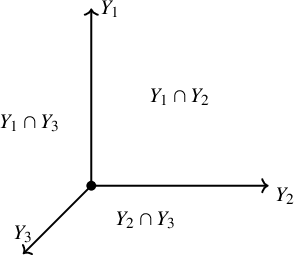


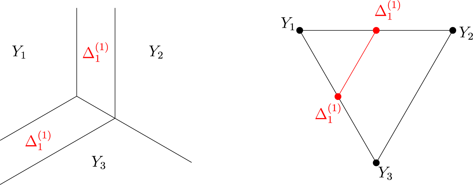


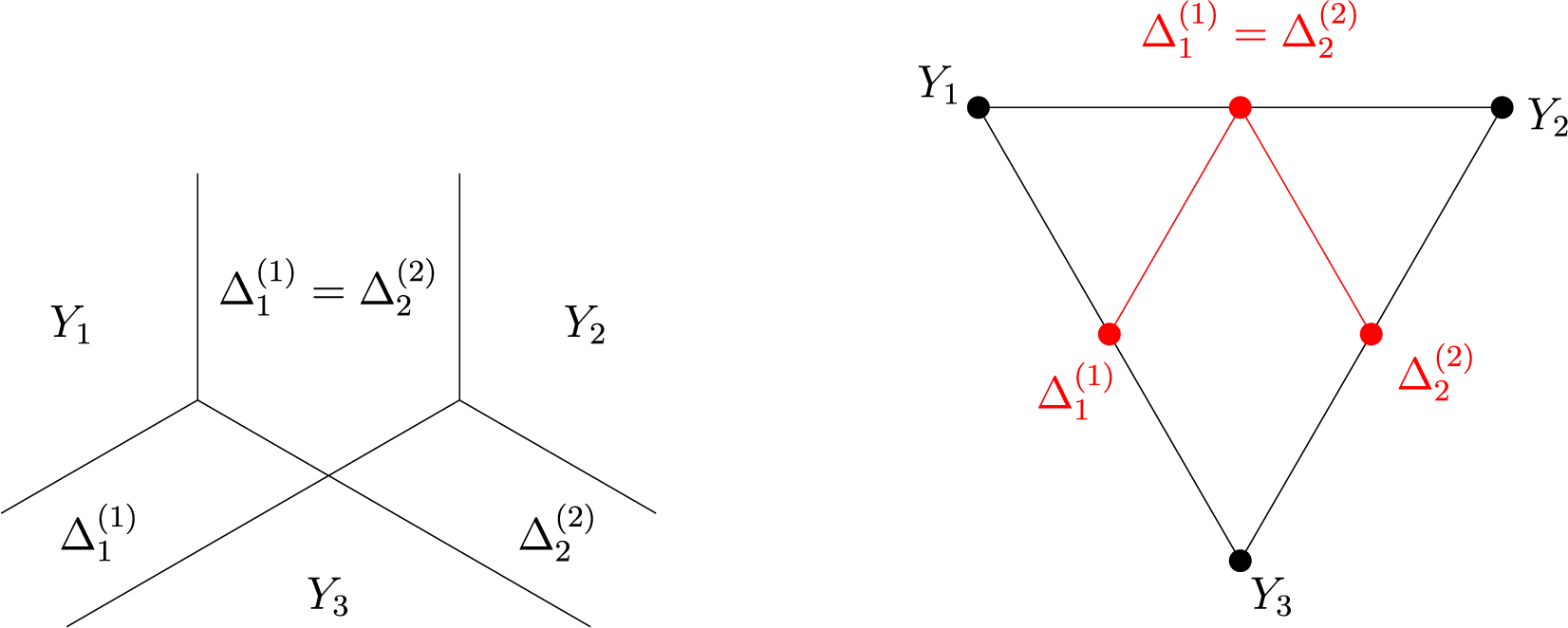


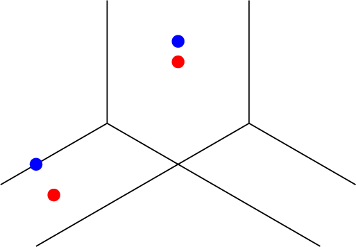


 Open access