


Impact statement
Understanding how blood flows inside the human heart is critical for improving cardiovascular diagnostics and treatments. This study explores how swirling blood flow patterns, known as vortex rings, form and evolve within the left ventricle, the chamber responsible for pumping oxygenated blood throughout the body. By using a combination of high-fidelity computer simulations and advanced data analysis tools, we identify the key flow structures that emerge during the filling phase of the heartbeat and how these are affected by heart geometry. Our approach also produces a highly efficient reduced-order model that can predict the future evolution of blood flow from only a short initial input. This has the potential to enable real-time simulations of cardiac function, which could assist clinicians in diagnosing heart dysfunction, designing patient-specific treatment plans or optimizing prosthetic heart devices. More broadly, this work bridges fundamental fluid mechanics with translational tools for healthcare and biomedical engineering.
1. Introduction
Cardiovascular diseases remain the leading cause of mortality worldwide, with heart failure representing a major source of morbidity and a significant reduction in quality of life (World Health Organization 2024). In this context, understanding and predicting intraventricular blood flow dynamics is essential to improving diagnosis, prognosis, and treatment planning in patients with cardiac dysfunction (see Kilner et al. Reference Kilner, Yang, Wilkes, Mohiaddin, Firmin and Yacoub2000; Thomas & Popovic Reference Thomas and Popovic2006). The left ventricle (LV), as the main pumping chamber of the heart, plays a central role in cardiac output, and its hemodynamics are intimately linked to both structural integrity and functional performance (Pedrizzetti & Domenichini Reference Pedrizzetti and Domenichini2015; Sengupta et al. Reference Sengupta, Korinek, Belohlavek, Narula, Vannan, Jahangir and Khandheria2006).
Computational fluid dynamics (CFD) has emerged as a powerful tool for investigating intraventricular flows, complementing in vivo measurements by enabling detailed, controllable exploration of flow patterns. Numerous studies have applied CFD to both idealized and patient-specific LV geometries, providing valuable insights into vortex dynamics, energy dissipation and wall shear stresses. For instance, Spandan et al. (Reference Spandan, Meschini, Ostilla-Mónico, Lohse, Querzoli, De Tullio and Verzicco2017) introduced a parallel interaction potential approach coupled with the immersed boundary method for fully resolved fluid–structure interaction simulations of deformable cardiac structures. This methodology has been extended to simulate healthy and pathological ventricles with natural and prosthetic mitral valves (Meschini et al. Reference Meschini, De Tullio, Querzoli and Verzicco2018), as well as to investigate systolic anterior motion in hypertrophic cardiomyopathy (Meschini, Mittal & Verzicco Reference Meschini, Mittal and Verzicco2021).
Domenichini et al. (Reference Domenichini, Pedrizzetti and Baccani2005) conducted early numerical studies on the three-dimensional inflow into a ventricular-shaped cavity. They later complemented this with experimental validation (Domenichini et al. Reference Domenichini, Querzoli, Cenedese and Pedrizzetti2007), providing deeper insights into the mechanisms driving intraventricular flow. More recently, they explored the interaction between myocardial motion and fluid dynamics, demonstrating how alterations in tissue displacement are reflected in hemodynamic force distributions (Domenichini & Pedrizzetti Reference Domenichini and Pedrizzetti2016). Quarteroni et al. (Reference Quarteroni, Lassila, Rossi and Ruiz-Baier2017) have developed advanced frameworks for cardiac modelling that combine electromechanics, fluid dynamics and patient-specific data (Africa et al. Reference Africa, Fumagalli, Bucelli, Zingaro, Fedele, Dede’ and Quarteroni2024; Quarteroni et al. Reference Quarteroni, Lassila, Rossi and Ruiz-Baier2017). These contributions reinforce the value of CFD as a predictive tool in cardiac research.
These works represent only a small sample of the growing body of literature. A comprehensive overview of CFD-based cardiac flow simulations, including their application to vortex ring (VR) analysis, is provided in the review by Nagargoje et al. (Reference Nagargoje, Lazpita, Garicano-Mena and Clainche2025). The VR forms during early diastolic filling and plays a critical role in the efficient reorientation of the blood influx towards the aortic valve throughout the cardiac cycle. Its formation and stability are closely tied to ventricular geometry, wall motion and pathological changes, making it a relevant biomarker for cardiovascular health. In a recent study (see Lazpita et al. Reference Lazpita, Neidlin, Garicano-Mena and Clainche2025), we analysed the physical mechanisms underlying VR dynamics in two idealized LV geometries, identifying the VR as the dominant flow structure driving the system’s temporal evolution and highlighting its potential as a diagnostic indicator.
Despite these advancements, generating high-fidelity CFD simulations of cardiac flows remains computationally demanding. The need to account for large deformations, moving boundaries and physiologically realistic conditions results in considerable computational cost. Moreover, many CFD solvers suffer from numerical instability when applied to complex ventricular geometries or pathological flow regimes, often requiring extensive tuning or simplification of the physical model. These challenges restrict the scope of CFD applications in both clinical and research contexts.
As a result, many studies are constrained to a limited number of cardiac cycles, often fewer than five, impeding the statistical robustness and generalizability of the resulting data (Kheradvar et al. Reference Kheradvar, Pedrizzetti, Kheradvar and Pedrizzetti2012; Chnafa et al. Reference Chnafa, Mendez and Nicoud2014). This limitation poses a significant barrier to the development of data-driven models, which require temporally rich datasets to achieve reliable performance across varying cardiac conditions.
In order to address these challenges, a novel reduced-order model (ROM) is proposed. This model is designed to accelerate the obtention of intraventricular flow databases as an alternative to high-fidelity CFD simulations. Although ROMs are widely used in fluid mechanics to reduce computational cost, their application to cardiac hemodynamics is still limited. This is mainly due to the complexity of the problem, which involves large deformations, moving boundaries, strong nonlinearities and fluid–structure interaction (Ballarin et al. Reference Ballarin, Faggiano, Ippolito, Manzoni, Quarteroni, Rozza and Scrofani2016; Lassila et al. Reference Lassila, Manzoni, Quarteroni and Rozza2014). Our method extends the capabilities of existing modal decomposition frameworks by leveraging the higher-order dynamic mode decomposition (HODMD) algorithm (Le Clainche & Vega Reference Le Clainche and Vega2017 a). The HODMD technique extracts the dominant coherent structures of the flow and models their temporal evolution. In doing so, it captures the underlying physics, most notably the VR dynamics that govern early diastolic filling in the LV.
Although HODMD has been successfully applied in simplified fluid scenarios, such as bluff body wakes or laminar shear flows (Le Clainche & Vega Reference Le Clainche and Vega2017 b), this work presents its first application, to the authors’ knowledge, to cardiac flows. In this context, we address additional challenges inherent to cardiac flow simulations, such as significant domain deformation driven by myocardial motion (i.e. involving moving meshes). These complexities are further augmented by the influence of the ventricular wall on VR dynamics, as well as by the substantial temporal variability in velocity and pressure fields throughout the cardiac cycle, driven by the strong coupling between geometry deformation and flow evolution. By adapting the ROM to the spatiotemporal characteristics of the data, we achieve significant computational savings while preserving the essential dynamics of the system.
Recent advances in deep learning have introduced a variety of architectures, such as autoencoders, convolutional neural networks and recurrent models, for data-driven flow reconstruction and ROM (Sanchis-Agudo et al. Reference Sanchis-Agudo, Wang, Arnau, Guastoni, Lim, Duraisamy and Vinuesa2024; Solera-Rico et al. Reference Solera-Rico, Vila, Gómez-López, Wang, Almashjary, Dawson and Vinuesa2024). These approaches can offer rapid predictions once trained, but they typically require a problem-specific network design and extensive hyperparameter tuning to ensure both numerical stability and physical consistency. In contrast, the HODMD framework employed in this study extracts dominant coherent structures and their characteristic frequencies directly from data, without the need for prior assumptions about the underlying dynamics or geometry. This provides a more interpretable, physics-grounded representation of the flow while maintaining competitive accuracy with significantly lower model complexity.
The following sections are structured as follows: § 2 introduces the ROM methodology based on HODMD and its implementation. Section 3 presents the two idealized LV databases used in this study. In § 4, we provide a detailed analysis of the ROM configuration using two distinct idealized LV geometries. Finally, § 5 summarizes the main findings and discusses future directions.
2. Reduced-order modelling
As mentioned, the ROM employed in this study is based on HODMD, a data-driven technique that extracts dominant spatiotemporal patterns from complex dynamical systems. To handle the inherently high-dimensional nature of the simulation data, we adopt a tensor-based extension of the algorithm, known as multidimensional HODMD (mdHODMD) (Hetherington et al. Reference Hetherington, Corrochano, Abadía-Heredia, Lazpita, Muñoz, Díaz, Maiora, López-Martín and Le Clainche2024). This formulation allows us to preserve the multidimensional structure of the dataset and enhance both computational efficiency and interpretability.
The input data consists of time-resolved three-dimensional velocity fields obtained from CFD simulations. For each time instant, the velocity field is represented by three components defined over a structured grid in three spatial directions. By stacking all temporal snapshots together, the dataset can be naturally arranged as a five-dimensional tensor $ \boldsymbol{V} \in \mathbb{R}^{J_1 \times J_2 \times J_3 \times J_4 \times K}$
, where
$ \boldsymbol{V} \in \mathbb{R}^{J_1 \times J_2 \times J_3 \times J_4 \times K}$
, where
-
(i) $ J_1 = 3$
corresponds to the velocity components
$ (v_x, v_y, v_z)$
,
$ J_1 = 3$
corresponds to the velocity components
$ (v_x, v_y, v_z)$
, -
(ii)
$ J_2, J_3, J_4$
represent the spatial discretization density along the three coordinate directions and -
(iii)
$ K$
denotes the number of time steps.


The mdHODMD algorithm is then applied to this tensor in three consecutive main steps: dimensionality reduction via tensor decomposition, extraction of dynamic modes and their associated frequencies, and prediction of the system’s temporal evolution.
2.1. Data dimensionality reduction
The processing of large-scale datasets directly poses a significant computational challenge, requiring the implementation of dimensionality reduction techniques to ensure manageability. Singular value decomposition (SVD) (Sirovich Reference Sirovich1987) is widely used in fluid dynamics to reduce data dimensionality and filter out noise. However, the intraventricular flow simulations considered in this work are high-dimensional, transient and highly nonlinear. They involve moving geometries subject to large temporal deformations and complex spatiotemporal patterns that appear. As a result, more advanced techniques are required to analyse and predict their behaviour effectively. In this study, we apply the high-order singular value decomposition (HOSVD) (Le Clainche & Vega Reference Le Clainche and Vega2017 a), a tensor-based extension of SVD that enables simultaneous decomposition along multiple data dimensions. This method improves compression and noise filtering by decoupling the modes in each dimension. As a result, it can distinguish and eliminate noise or redundancies independently across spatial, temporal and physical-magnitude components. Such enhanced denoising and compression capabilities make HOSVD particularly well-suited for building robust, low-rank representations from transient flow data (Groun et al. Reference Groun, Villalba-Orero, Casado-Martín, Lara-Pezzi, Valero, Le Clainche and Garicano-Mena2025), thereby supporting the construction of accurate and efficient predictive models.
The HOSVD is applied to the fifth-dimensional tensor $\mathbf{V}$
, which in turn is factorized as
$\mathbf{V}$
, which in turn is factorized as
 \begin{equation} \mathbf{V}_{j_1j_2j_3j_4k} \simeq \sum _{p_1=1}^{P_1}\sum _{p_2=1}^{P_2}\sum _{p_3=1}^{P_3}\sum _{p_4=1}^{P_4} \sum _{n=1}^{N} \mathbf{S}_{p_1p_2p_3p_4n} \mathbf{W}^{(v)}_{j_1p_1}\mathbf{W}^{(x)}_{j_2p_2} \mathbf{W}^{(y)}_{j_3p_3}\mathbf{W}^{(z)}_{j_4p_4}\mathbf{T}_{kn}, \end{equation}
where $\mathbf{S}_{p_1p_2p_3p_4n}$
is the fifth-dimensional core tensor, and the orthonormal matrices
$\mathbf{S}_{p_1p_2p_3p_4n}$
is the fifth-dimensional core tensor, and the orthonormal matrices $\mathbf{W}^{(v)}$
,
$\mathbf{W}^{(v)}$
, $\mathbf{W}^{(x)}$
,
$\mathbf{W}^{(x)}$
, $\mathbf{W}^{(y)}$
,
$\mathbf{W}^{(y)}$
, $\mathbf{W}^{(z)}$
and
$\mathbf{W}^{(z)}$
and $\mathbf{T}$
contain the SVD modes for each dimension. A tuneable tolerance
$\mathbf{T}$
contain the SVD modes for each dimension. A tuneable tolerance $ \varepsilon$
determines the number of retained modes
$ \varepsilon$
determines the number of retained modes $ N$
, ensuring that
$ N$
, ensuring that $ \sigma _{N +1}^{(j)}/\sigma _1^{(j)} \leq \varepsilon _1$
with
$ \sigma _{N +1}^{(j)}/\sigma _1^{(j)} \leq \varepsilon _1$
with $j = 1,\ldots ,5$
. This temporal matrix
$j = 1,\ldots ,5$
. This temporal matrix $\mathbf{T}$
containing the temporal coefficients associated with each mode (of dimensions
$\mathbf{T}$
containing the temporal coefficients associated with each mode (of dimensions $N \times K$
) serves as input for the subsequent dynamic mode decomposition (DMD) computation.
$N \times K$
) serves as input for the subsequent dynamic mode decomposition (DMD) computation.
2.2. Calculation of DMD modes
Dynamic mode decomposition (Schmid Reference Schmid2010) provides a ROM approach by expressing complex spatiotemporal data as a linear combination of $ M$
coherent structures, or modes, that evolve in time. The approximation of the dataset
$ M$
coherent structures, or modes, that evolve in time. The approximation of the dataset $ \mathbf{V}_{j_1}(x,y,z,t_k)$
(where
$ \mathbf{V}_{j_1}(x,y,z,t_k)$
(where $ j_1=1,\ldots ,3$
indexes the velocity components) is formulated as
$ j_1=1,\ldots ,3$
indexes the velocity components) is formulated as
 \begin{equation} \mathbf{V}_{j_1}(x,y,z,t_k) \approx \sum _{m=1}^{M} a_m \, \mathbf{u}_m(x,y,z) \, e^{(\delta _m + i\omega _m)t_k} \quad \text{for} \; k=1,\ldots ,K \, , \end{equation}
where $ \mathbf{u}_m$
denotes the spatial structure of each DMD mode,
$ \mathbf{u}_m$
denotes the spatial structure of each DMD mode, $ a_m$
is the mode amplitude,
$ a_m$
is the mode amplitude, $ \delta _m$
is the temporal growth rate and
$ \delta _m$
is the temporal growth rate and $ \omega _m$
represents the oscillation frequency.
$ \omega _m$
represents the oscillation frequency.
To obtain these modes, DMD assumes a linear mapping between consecutive data snapshots $ \{ \mathbf{v}_1, \mathbf{v}_2, \ldots , \mathbf{v}_K \}$
, posing the relation to be described as
$ \{ \mathbf{v}_1, \mathbf{v}_2, \ldots , \mathbf{v}_K \}$
, posing the relation to be described as
 \begin{equation} \mathbf{V}_2^{K} \approx \mathbf{R} \, \mathbf{V}_1^{K-1} \, , \end{equation}
where $ \mathbf{R}$
is a linear operator that approximates the underlying dynamics, effectively capturing the temporal progression through the so-called Koopman framework (Mezić Reference Mezić2013; Otto & Rowley Reference Otto and Rowley2021).
$ \mathbf{R}$
is a linear operator that approximates the underlying dynamics, effectively capturing the temporal progression through the so-called Koopman framework (Mezić Reference Mezić2013; Otto & Rowley Reference Otto and Rowley2021).
Higher-order DMD (Le Clainche & Vega Reference Le Clainche and Vega2017
a) extends standard DMD by incorporating multiple time-delayed snapshots, enhancing robustness and accuracy in capturing complex flow structures. Furthermore, the mdHODMD algorithm preserves the tensorial formulation by applying the higher-order Koopman assumption to the temporal matrix $\mathbf{T}$
extracted in the previous step using HOSVD (see (2.1)) as
$\mathbf{T}$
extracted in the previous step using HOSVD (see (2.1)) as
 \begin{equation} \mathbf{T}_{d+1}^K \approx \widehat {\mathbf{R}}_1 \mathbf{T}_1^{K-d}+ \widehat {\mathbf{R}}_2 \mathbf{T}_2^{K-d+1} + \cdots + \widehat {\mathbf{R}}_d \mathbf{T}_d^{K-1}. \end{equation}
This formulation links each snapshot to $d$
previous time steps, capturing intricate temporal dynamics beyond what standard DMD offers. The modified Koopman matrix
$d$
previous time steps, capturing intricate temporal dynamics beyond what standard DMD offers. The modified Koopman matrix $\widehat {\mathbf{R}}$
, which contains all the linear operators (
$\widehat {\mathbf{R}}$
, which contains all the linear operators ( $ \hat {R_1}, \hat {R_2}, \ldots , \hat {R_d}$
), is then computed to extract the DMD modes. Another tuneable tolerance is introduced for the HODMD; in this work, and following the guidelines discussed in Le Clainche & Vega (Reference Le Clainche and Vega2017
a) and Hetherington et al. (Reference Hetherington, Corrochano, Abadía-Heredia, Lazpita, Muñoz, Díaz, Maiora, López-Martín and Le Clainche2024) which is set equal to the one selected for the HOSVD, such that
$ \hat {R_1}, \hat {R_2}, \ldots , \hat {R_d}$
), is then computed to extract the DMD modes. Another tuneable tolerance is introduced for the HODMD; in this work, and following the guidelines discussed in Le Clainche & Vega (Reference Le Clainche and Vega2017
a) and Hetherington et al. (Reference Hetherington, Corrochano, Abadía-Heredia, Lazpita, Muñoz, Díaz, Maiora, López-Martín and Le Clainche2024) which is set equal to the one selected for the HOSVD, such that $ \varepsilon _1 = \varepsilon _2 = \varepsilon$
.
$ \varepsilon _1 = \varepsilon _2 = \varepsilon$
.
2.3. Prediction
Once the data is decomposed into DMD modes, future-state predictions are obtained by evaluating (2.2) at time instants beyond the training window $ t \gt t_K$
. Specifically, the model is constructed using data within the interval
$ t \gt t_K$
. Specifically, the model is constructed using data within the interval $ t \in [0,\, pT]$
, where
$ t \in [0,\, pT]$
, where $ T$
is the period of the cardiac cycle and
$ T$
is the period of the cardiac cycle and $ p$
is the number of cycles employed for training. In this work, we will consider
$ p$
is the number of cycles employed for training. In this work, we will consider $ p \in \mathbb{R}$
and
$ p \in \mathbb{R}$
and $p\leq 10$
. The resulting ROM is then used to predict the flow dynamics in a later interval, namely
$p\leq 10$
. The resulting ROM is then used to predict the flow dynamics in a later interval, namely $ t \in [10T,\, 20T]$
, allowing us to assess the long-term predictive capabilities of the method.
$ t \in [10T,\, 20T]$
, allowing us to assess the long-term predictive capabilities of the method.
The way modes are selected plays a crucial role in ensuring prediction accuracy and stability in the model. Depending on the calibration of the algorithm, spurious modes unrelated to the underlying physics may be captured, typically associated with noise or numerical artefacts. As a result, using all computed $ M$
DMD modes can degrade the quality of the extrapolated prediction. To address this difficulty, we adopt a filtering strategy in which only those modes with growth rates lower than a certain threshold are deemed physically relevant and retained for prediction. This threshold is set with a tuneable growth rate value
$ M$
DMD modes can degrade the quality of the extrapolated prediction. To address this difficulty, we adopt a filtering strategy in which only those modes with growth rates lower than a certain threshold are deemed physically relevant and retained for prediction. This threshold is set with a tuneable growth rate value $ \delta _{tune}$
. Thus, stable modes will correspond to
$ \delta _{tune}$
. Thus, stable modes will correspond to $ -\delta _{tune} \lt \delta _m\lt 0$
with
$ -\delta _{tune} \lt \delta _m\lt 0$
with $\delta _{tune}\gt 0$
. Almost all of the selected modes correspond to frequencies associated with the dominant dynamics of the system.
$\delta _{tune}\gt 0$
. Almost all of the selected modes correspond to frequencies associated with the dominant dynamics of the system.
Furthermore, when working with transient simulation data, certain modes, although physically relevant, may exhibit highly negative growth rates, leading to their rapid attenuation over time. This offers the potential to enhance the temporal stability of the model predictions; we also construct an alternative formulation in which we enforce $ \delta _m = 0$
, thereby eliminating exponential decay. This modification prevents excessive damping of key flow structures and enables more reliable long-term forecasts of the intraventricular dynamics.
$ \delta _m = 0$
, thereby eliminating exponential decay. This modification prevents excessive damping of key flow structures and enables more reliable long-term forecasts of the intraventricular dynamics.
To assess the accuracy of the ROM, we analyse the absolute error distribution over the entire dataset by computing the histogram of the normalized absolute error, defined as
 \begin{equation} E(\%) = \frac {|\textbf {v} - \textbf {v}_{\text{pred}}|}{\max |\textbf {v} - \textbf {v}_{\text{pred}}|} \times 100, \end{equation}
where $\textbf {v}$
denotes the reference simulation data and
$\textbf {v}$
denotes the reference simulation data and $\textbf {v}_{\text{pred}}$
is the reconstructed prediction. The normalization factor corresponds to the maximum absolute error computed independently for each velocity component, considering all spatial locations and time steps in the domain.
$\textbf {v}_{\text{pred}}$
is the reconstructed prediction. The normalization factor corresponds to the maximum absolute error computed independently for each velocity component, considering all spatial locations and time steps in the domain.
The number of bins in the histogram is determined using Sturges’s formula, applied to the spatial grid,
 \begin{equation} N_{\text{bins}} = 1 + \log _2(N_{\text{grid}}), \end{equation}
where $N_{\text{grid}} = N_x \times N_y \times N_z$
represents the total number of spatial points. In our case, this results in approximately 20 bins, allowing for an intuitive interpretation: the first bin represents the relative frequency of errors within the range 0 %–5 %, the second within 5 %–10 %, and so forth.
$N_{\text{grid}} = N_x \times N_y \times N_z$
represents the total number of spatial points. In our case, this results in approximately 20 bins, allowing for an intuitive interpretation: the first bin represents the relative frequency of errors within the range 0 %–5 %, the second within 5 %–10 %, and so forth.
A key advantage of the ROM is its drastic reduction in computational cost. In this study, this increase in computational efficiency is quantified using the speed-up factor (SUF), defined as
 \begin{equation} \text{SUF} = \frac {t_{{\rm CFD}} \times N_{{\rm CPU}}}{t_{{\rm ROM}}} \end{equation}
where $t_{\text{CFD}}$
is the runtime of the full-order CFD simulation,
$t_{\text{CFD}}$
is the runtime of the full-order CFD simulation, $N_{\text{CPU}}$
is the number of processors used, and
$N_{\text{CPU}}$
is the number of processors used, and $t_{\text{ROM}}$
is the time required for the ROM prediction.
$t_{\text{ROM}}$
is the time required for the ROM prediction.
Finally, we note that the HODMD-based ROM involves several tuneable parameters that require careful calibration. These include the truncation tolerance $\varepsilon$
, which controls the number of modes retained; the window size
$\varepsilon$
, which controls the number of modes retained; the window size $d$
, which determines the number of snapshots used in each HODMD window; and the threshold
$d$
, which determines the number of snapshots used in each HODMD window; and the threshold $\delta _{tune}$
applied to the growth rates to distinguish physically relevant modes from spurious ones. To calibrate the ROM, multiple combinations of
$\delta _{tune}$
applied to the growth rates to distinguish physically relevant modes from spurious ones. To calibrate the ROM, multiple combinations of $\varepsilon$
and
$\varepsilon$
and $d$
are explored during training. While
$d$
are explored during training. While $\varepsilon$
is adjusted depending on the noise level,
$\varepsilon$
is adjusted depending on the noise level, $d$
is typically chosen between 15 %–50 % of the total snapshots. Once the physical modes are identified, their growth rates and frequencies are analysed to set an appropriate threshold
$d$
is typically chosen between 15 %–50 % of the total snapshots. Once the physical modes are identified, their growth rates and frequencies are analysed to set an appropriate threshold $\delta _{tune}$
, ensuring that only persistent, physically meaningful modes are retained for prediction. This procedure enhances the robustness and accuracy of the resulting ROM.
$\delta _{tune}$
, ensuring that only persistent, physically meaningful modes are retained for prediction. This procedure enhances the robustness and accuracy of the resulting ROM.
To calibrate the HODMD-based ROM, multiple combinations of the truncation tolerance $\varepsilon$
and the window size
$\varepsilon$
and the window size $d$
are explored. The tolerance
$d$
are explored. The tolerance $\varepsilon$
is adjusted depending on the noise present in the data, whereas
$\varepsilon$
is adjusted depending on the noise present in the data, whereas $d$
is typically chosen to be between 10 %–50 % of the total snapshots (Le Clainche et al. Reference Le Clainche, Izbassarov, Rosti, Brandt and Tammisola2020; Hetherington et al. Reference Hetherington, Corrochano, Abadía-Heredia, Lazpita, Muñoz, Díaz, Maiora, López-Martín and Le Clainche2024). After identifying the physical modes, their growth rates and frequencies are analysed to define a threshold that separates persistent modes from spurious ones, ensuring the robustness of the ROM construction.
$d$
is typically chosen to be between 10 %–50 % of the total snapshots (Le Clainche et al. Reference Le Clainche, Izbassarov, Rosti, Brandt and Tammisola2020; Hetherington et al. Reference Hetherington, Corrochano, Abadía-Heredia, Lazpita, Muñoz, Díaz, Maiora, López-Martín and Le Clainche2024). After identifying the physical modes, their growth rates and frequencies are analysed to define a threshold that separates persistent modes from spurious ones, ensuring the robustness of the ROM construction.
3. Flow dynamics
To evaluate the performance of the ROM introduced earlier, we apply it to two distinct datasets, both representing idealized LV geometries. The first model, referred to as Ideal 1, consists of a semiellipsoidal chamber extracted from Zheng et al. (Reference Zheng, Seo, Vedula, Abraham and Mittal2012) and will be used to develop and illustrate the methodology. The second model, Ideal 2, has a smoother, more rounded chamber shape and has been studied in prior works (Vedula et al. Reference Vedula, Fortini, Seo, Querzoli and Mittal2014; Kjeldsberg, Sundnes & Valen-Sendstad Reference Kjeldsberg, Sundnes and Valen-Sendstad2023). This model will serve as an additional test case to evaluate the robustness of the approach under different conditions.
3.1. Database
To ensure that the idealized geometries represent physiologically realistic left ventricular conditions, particularly the end-systolic volume that corresponds to the minimum volume at the end of systole, we define a set of non-dimensional geometric parameters. These parameters are expressed in table 1 using the base radius $ a$
of the ventricular chamber as the reference length for each model.
$ a$
of the ventricular chamber as the reference length for each model.
Non-dimensional geometric parameters for the two idealized ventricular models, using base radius $ a$
as reference length.
$ a$
as reference length.

A schematic representation of these parameters and their spatial arrangement is provided in figure 1, illustrating the geometry and orientation of each feature. The figure also identifies the symmetry plane A–A’ (located at $y=0$
) used throughout the analysis (highlighted in blue). Additionally, a probe line (L1), indicated in red, is defined to extract temporal data at specific spatial locations. For the Ideal 1 model, L1 is located at
$y=0$
) used throughout the analysis (highlighted in blue). Additionally, a probe line (L1), indicated in red, is defined to extract temporal data at specific spatial locations. For the Ideal 1 model, L1 is located at $ x/a = 0, \, y/a = 0$
, and it extends through all the vertical
$ x/a = 0, \, y/a = 0$
, and it extends through all the vertical $z$
of the chamber. For the Ideal 2 model, L1 is positioned at
$z$
of the chamber. For the Ideal 2 model, L1 is positioned at $ x/a = 0, \, y/a = 0$
, and again it takes all the chamber height.
$ x/a = 0, \, y/a = 0$
, and again it takes all the chamber height.
Representation of both idealized LV models: (a) Ideal 1 and (b) Ideal 2. Blue, symmetry plane A–A’ used for two-dimensional visualization; red, probe line L1 to represent temporal data.

Using the two idealized geometries of the LV, we conducted CFD simulations to investigate intraventricular flow dynamics. Simulations were carried out using the solver Ansys Fluent (Ansys, Inc. 2023). In both cases, blood was modelled as an incompressible Newtonian fluid with constant density $\rho = 1060\,\text{kg m}^{-3}$
and dynamic viscosity
$\rho = 1060\,\text{kg m}^{-3}$
and dynamic viscosity $\mu = 0.004\,\text{Pa}\, \text{s}$
.
$\mu = 0.004\,\text{Pa}\, \text{s}$
.
To characterize the flow regime, we computed the Reynolds number ( $\textit{Re}$
) based on the inlet tube diameter
$\textit{Re}$
) based on the inlet tube diameter $D$
(non-dimensionalized as
$D$
(non-dimensionalized as $D/a$
) and the peak inlet velocity
$D/a$
) and the peak inlet velocity $V_{\text{max}}$
over the cardiac cycle. The resulting Reynolds numbers were approximately
$V_{\text{max}}$
over the cardiac cycle. The resulting Reynolds numbers were approximately $\textit{Re} \approx 5500$
for the Ideal 1 model and
$\textit{Re} \approx 5500$
for the Ideal 1 model and $\textit{Re} \approx 4900$
for Ideal 2. Despite these values indicating transitional or potentially turbulent flow, we assumed a laminar regime, in line with previous studies (He et al. Reference He, Han, Zhang, Shah, Kaczorowski, Griffith and Wu2022; Tagliabue, Dedè & Quarteroni Reference Tagliabue, Dedè and Quarteroni2017), where coherent vortex structures, such as the main VR, were accurately captured under laminar assumptions.
$\textit{Re} \approx 4900$
for Ideal 2. Despite these values indicating transitional or potentially turbulent flow, we assumed a laminar regime, in line with previous studies (He et al. Reference He, Han, Zhang, Shah, Kaczorowski, Griffith and Wu2022; Tagliabue, Dedè & Quarteroni Reference Tagliabue, Dedè and Quarteroni2017), where coherent vortex structures, such as the main VR, were accurately captured under laminar assumptions.
A zero-velocity initial condition is set in the simulation pipeline for both models. Moreover, for both simulations, pressure-based boundary conditions were set at the inlet and outlet. These boundaries dynamically alternated between open and closed states to represent the cardiac cycle: during diastole, the inlet was open and the outlet treated as a wall; during systole, the roles were reversed. This boundary-switching was complemented by the dynamic motion of the ventricular wall, imposed by prescribing an interpolated sequence of meshes corresponding to each time instant. This approach induces pressure gradients within the chamber that drive blood in and out, thereby mimicking physiological behaviour.
The simulation framework and its assumptions were extensively validated in previous studies (Lazpita et al. Reference Lazpita, Garicano-Mena, Paniagua, Le Clainche and Valero2024 a,b, Reference Lazpita, Neidlin, Garicano-Mena and Clainche2025), including convergence analyses and comparisons with benchmark data. All numerical simulations were performed on the high-performance computing cluster Magerit, hosted at CeSViMa (Centro de Supercomputación y Visualización de Madrid). The computations were parallelized using 40 message passing interface (MPI) tasks within a single node.
For the rest of the manuscript, time is non-dimensionalized using the period $ T$
, such that
$ T$
, such that $ t^* = t/T$
. This normalization allows for a consistent comparison of corresponding time instants across both simulation databases. It is also important to note that, for the first geometry, the diastolic phase takes place within the interval
$ t^* = t/T$
. This normalization allows for a consistent comparison of corresponding time instants across both simulation databases. It is also important to note that, for the first geometry, the diastolic phase takes place within the interval $ t^* \in [i,\, i + 0.67]$
, followed by the systolic phase in
$ t^* \in [i,\, i + 0.67]$
, followed by the systolic phase in $ t^* \in [i + 0.67,\, i + 1]$
. In contrast, for the second geometry, diastole spans
$ t^* \in [i + 0.67,\, i + 1]$
. In contrast, for the second geometry, diastole spans $ t^* \in [i,\, i + 0.8]$
, and systole occurs within
$ t^* \in [i,\, i + 0.8]$
, and systole occurs within $ t^* \in [i + 0.8,\, i + 1]$
, where
$ t^* \in [i + 0.8,\, i + 1]$
, where $ i$
denotes the cycle index.
$ i$
denotes the cycle index.
A key aspect of intraventricular hemodynamics is the formation and evolution of a VR during diastole, triggered by the inflow through the mitral valve (Nagargoje et al. Reference Nagargoje, Lazpita, Garicano-Mena and Clainche2025). This structure undergoes tilting and eventual breakdown due to instabilities, and its dynamics are considered a primary indicator of pumping efficiency. Accurately capturing the VR behaviour is, therefore, essential.
Figure 2 illustrates representative time instants for both geometries. The green isocontours show the Q-criterion at a level of 2500, highlighting vortex cores, while the colormap on the symmetry plane displays the out-of-plane vorticity in the range $[-100, 100] \: \text{s}^{-1}$
. Notably, the VR in Ideal 1 dissipates earlier than in Ideal 2; by
$[-100, 100] \: \text{s}^{-1}$
. Notably, the VR in Ideal 1 dissipates earlier than in Ideal 2; by $ t^* = 0.25$
, the ring in Ideal 1 is already breaking up, whereas Ideal 2 still maintains a coherent and smooth structure. Even at
$ t^* = 0.25$
, the ring in Ideal 1 is already breaking up, whereas Ideal 2 still maintains a coherent and smooth structure. Even at $ t^* = 0.40$
, the second model, though deformed, maintains a closed VR, while the first model’s ring has fully dissipated.
$ t^* = 0.40$
, the second model, though deformed, maintains a closed VR, while the first model’s ring has fully dissipated.
As shown in Lazpita et al. (Reference Lazpita, Neidlin, Garicano-Mena and Clainche2025), the vortex breakdown process is strongly influenced by ventricular geometry. In the Ideal 1 configuration, which features a narrower chamber, the vortex interacts with the ventricular wall at an earlier stage. This early interaction triggers the breakdown process before the VR can reach the apex. In contrast, the Ideal 2 model, with a wider chamber, allows the VR to fully develop, travel towards the apex, and break down as a combination of a reduction in velocity and wall interaction.
Representative snapshots of the intraventricular flow fields for Ideal 1 (a) and Ideal 2 (b). Green, Q-criterion isosurface at 2500; background, vorticity in the symmetry plane; range $[-100, 100]$
.
$[-100, 100]$
.

These contrasting behaviours can be attributed to two main factors:
-
(i) the narrower geometry of Ideal 1 causes the vortex to interact more strongly with the ventricular walls, preventing it from reaching the apex and accelerating its breakdown;
-
(ii) Ideal 2 exhibits a lower ejection fraction and volume change, resulting in reduced pressure gradients and slower flow dynamics.
These differences in VR dynamics will be key for assessing the ROM’s ability to capture flow physics across varying conditions.
Each simulation database consists of 20 cardiac cycles, with flow fields sampled at a time interval of $ \Delta t^* = 0.05$
: therefore, these are 20 snapshots per cycle and a total of
$ \Delta t^* = 0.05$
: therefore, these are 20 snapshots per cycle and a total of $ K = 400$
snapshots. For training the ROM, we use data from the first 10 cycles, which include the initial transient phase. The remaining 10 cycles are reserved for validation, as they capture the dynamics once the system has reached temporal convergence. This distinction is further supported by the application of DMD, which reveals that growth rates stabilize only in the latter cycles.
$ K = 400$
snapshots. For training the ROM, we use data from the first 10 cycles, which include the initial transient phase. The remaining 10 cycles are reserved for validation, as they capture the dynamics once the system has reached temporal convergence. This distinction is further supported by the application of DMD, which reveals that growth rates stabilize only in the latter cycles.
Although it is common practice in the literature to simulate up to six cycles, we shall find that the flow remains in a transient state at that point (Canè et al. Reference Canè, Delcour, Luigi Redaelli, Segers and Degroote2022; Grünwald et al. Reference Grünwald, Korte, Wilmanns, Winkler, Linden, Herberg, Groß-Hardt, Steinseifer and Neidlin2022; Korte et al. Reference Korte, Rauwolf, Thiel, Mitrasch, Groschopp, Neidlin, Schmeißer, Braun-Dullaeus and Berg2023). This highlights the importance of longer simulations to ensure the reliability of the ROM and the physical relevance of the extracted modes.
The cases listed in table 2 are analogous for both LV geometries and thus we maintain the same denomination for consistency and brevity. Each case corresponds to a specific time window and number of cycles, which are used either for training or validation of the ROM. We also report the tuneable growth rate value selected for each case, which enables the identification of persistent modes that represent the main dynamics of the system, effectively discarding the spurious modes extracted by HODMD.
Summary of simulation cases used to build and evaluate the ROM discussed in § 2, including the number of cardiac cycles $p$
, normalized time intervals
$p$
, normalized time intervals $ t^*$
, snapshot count
$ t^*$
, snapshot count $K$
, their intended purpose and the selected tuneable growth rate parameter
$K$
, their intended purpose and the selected tuneable growth rate parameter $ \delta _{tune}$
.
$ \delta _{tune}$
.

3.2. Database sensitivity assessment
Despite careful simulation set-up, the complex nature of moving-wall CFD simulations introduces inherent variability across cycles, even setting the boundary conditions perfectly periodic (Chnafa et al. Reference Chnafa, Mendez and Nicoud2014). While major flow structures, such as the primary VR, secondary vortices and outflow jets, are consistently reproduced, smaller-scale features might vary.
We quantify the variability across cardiac cycles by analysing the cycle-to-cycle variation of the total kinetic energy (TKE), defined at each non-dimensional time instant $ t^*$
as
$ t^*$
as
 \begin{equation} \mathrm{TKE}(t^*) = \int _{V(t^*)} \frac {1}{2}\rho \mathbf{v}^2\, \text{d}V, \end{equation}
where $ V(t^*)$
is the time-dependent ventricular volume,
$ V(t^*)$
is the time-dependent ventricular volume, $ \rho$
is the fluid density, and
$ \rho$
is the fluid density, and $ \mathbf{v}$
is the velocity vector. The TKE integrated over each cardiac cycle is computed as
$ \mathbf{v}$
is the velocity vector. The TKE integrated over each cardiac cycle is computed as
 \begin{equation} \mathrm{TKE}_i = \int _{i-1}^{i} \mathrm{TKE}(t^*)\, \text{d}t^*, \quad i = 1, \ldots , 20, \end{equation}
where $ i$
, again, denotes the index of the cycle. To measure convergence and variability, we evaluate the relative root mean square error (RRMSE) of each cycle with respect to the last one,
$ i$
, again, denotes the index of the cycle. To measure convergence and variability, we evaluate the relative root mean square error (RRMSE) of each cycle with respect to the last one,
 \begin{equation} \mathrm{RRMSE}_{\mathrm{TKE}}(\%) = \frac {|\mathrm{TKE}_{20} - \mathrm{TKE}_i|}{|\mathrm{TKE}_{20}|} \times 100, \end{equation}
where $ \mathrm{TKE}_{20}$
is the integrated kinetic energy for the 20th cycle, considered as the reference.
$ \mathrm{TKE}_{20}$
is the integrated kinetic energy for the 20th cycle, considered as the reference.
Figure 3 illustrates the cycle-to-cycle variability in TKE error, expressed as the RRMSE for both Ideal 1 and Ideal 2 geometries. Remember that the simulation was initialized from a zero-velocity condition. After the initial transient, the RRMSE remains below 4 % across all subsequent cycles, indicating good reproducibility of global flow features. However, local flow characteristics, such as instantaneous velocity fields, may still exhibit larger discrepancies due to intrinsic variability in the numerical solution (Chnafa et al. Reference Chnafa, Mendez and Nicoud2014; Canè et al. Reference Canè, Delcour, Luigi Redaelli, Segers and Degroote2022). As such, predictions obtained from ROMs should be interpreted within a baseline uncertainty margin of approximately 5 %–10 %.
Cycle-to-cycle RRMSE of TKE for Ideal 1 and Ideal 2, visualized using a grouped bar plot.

Spectrum of DMD modes for both idealized models: normalized amplitude versus frequency (a) and absolute value of growth rate versus frequency (b). The dashed line at $ \delta _{tune} = 5 \times 10^{-2}$
in (b) separates persistent physical modes from transient or spurious ones.
$ \delta _{tune} = 5 \times 10^{-2}$
in (b) separates persistent physical modes from transient or spurious ones.

3.3. True frequency analysis
Figure 4 presents the DMD spectra obtained from a representative HODMD calibration applied to both Ideal 1 and Ideal 2 cases. Figure 4(a) shows the normalized amplitude of each mode with respect to frequency, while figure 4(b) displays the corresponding absolute values of the growth rates. Although only one calibration is depicted here for clarity, the modes shown have been previously identified as robust through an exhaustive sensitivity analysis involving the HODMD parameters $d$
and
$d$
and $\varepsilon$
, following the methodology described in Le Clainche et al. (Reference Le Clainche, Izbassarov, Rosti, Brandt and Tammisola2020) and Hetherington et al. (Reference Hetherington, Corrochano, Abadía-Heredia, Lazpita, Muñoz, Díaz, Maiora, López-Martín and Le Clainche2024).
$\varepsilon$
, following the methodology described in Le Clainche et al. (Reference Le Clainche, Izbassarov, Rosti, Brandt and Tammisola2020) and Hetherington et al. (Reference Hetherington, Corrochano, Abadía-Heredia, Lazpita, Muñoz, Díaz, Maiora, López-Martín and Le Clainche2024).
The amplitude spectra in figure 4(a) reveal the dominant frequencies that appear consistently across both geometries. These include the fundamental frequency $\omega = 2\pi$
and its harmonics, such as
$\omega = 2\pi$
and its harmonics, such as $4\pi$
,
$4\pi$
, $6\pi$
and up to approximately
$6\pi$
and up to approximately $14\pi$
, indicating strong periodicity and physical relevance of these modes. Lower-amplitude modes, scattered throughout the spectrum, are not persistent across calibrations and are interpreted as numerical noise or transient artefacts.
$14\pi$
, indicating strong periodicity and physical relevance of these modes. Lower-amplitude modes, scattered throughout the spectrum, are not persistent across calibrations and are interpreted as numerical noise or transient artefacts.
Figure 4(b) provides additional insight through the analysis of growth rates $|\delta _m|$
. Robust physical modes tend to have small or nearly zero-growth rates, indicating long-term persistence throughout the simulation. A threshold of
$|\delta _m|$
. Robust physical modes tend to have small or nearly zero-growth rates, indicating long-term persistence throughout the simulation. A threshold of $ \delta _{\text{tune}} = 5 \times 10^{-2}$
(shown as a dashed line) distinguishes these physical modes from the spurious ones, which exhibit larger decay or amplification rates and lack consistency. This threshold was established based on a qualitative shift observed in the spectral structure during the calibration study: below this value, the modes were consistently identified and physically meaningful, while above it, the spectrum became irregular and inconsistent.
$ \delta _{\text{tune}} = 5 \times 10^{-2}$
(shown as a dashed line) distinguishes these physical modes from the spurious ones, which exhibit larger decay or amplification rates and lack consistency. This threshold was established based on a qualitative shift observed in the spectral structure during the calibration study: below this value, the modes were consistently identified and physically meaningful, while above it, the spectrum became irregular and inconsistent.
These results confirm that the dominant dynamics of both Ideal 1 and Ideal 2 models are governed by a limited number of coherent structures oscillating at fundamental and harmonic frequencies, in agreement with the known periodicity of the cardiac cycle.
While the current study focuses on filtering spurious modes to construct a robust ROM, a detailed analysis of the retained modes and their physical interpretation is presented in a complementary work (Lazpita et al. Reference Lazpita, Neidlin, Garicano-Mena and Clainche2025), where the underlying flow dynamics in idealized LV models are extensively characterized. In that study, the leading modes were shown to capture the formation, tilting, and breakdown of the primary VR generated during early diastole, associated with the fundamental frequency $\omega = 2\pi$
, as well as the appearance of a secondary VR during the late diastolic inflow (
$\omega = 2\pi$
, as well as the appearance of a secondary VR during the late diastolic inflow ( $\omega = 4\pi$
). Higher-order modes revealed nonlinear interactions between these frequencies, describing the onset of vortex breakdown and the emergence of smaller-scale structures. This modal hierarchy thus provides a physically consistent picture of the intraventricular flow, linking coherent structures to characteristic temporal dynamics.
$\omega = 4\pi$
). Higher-order modes revealed nonlinear interactions between these frequencies, describing the onset of vortex breakdown and the emergence of smaller-scale structures. This modal hierarchy thus provides a physically consistent picture of the intraventricular flow, linking coherent structures to characteristic temporal dynamics.
4. Results
4.1. Semiellipsoidal model Ideal 1
For the first model, HODMD is applied to analyse several training subsets, each consisting of a varying number of cardiac cycles $p$
as defined in table 2. The objective is to determine how many cycles are necessary to accurately capture the temporal dynamics of the system. To evaluate this, we construct the temporal evolution of the system using the frequencies and growth rates extracted using HODMD. We consider two scenarios: (i) using the growth rates computed by HODMD, and (ii) setting all growth rates to zero.
$p$
as defined in table 2. The objective is to determine how many cycles are necessary to accurately capture the temporal dynamics of the system. To evaluate this, we construct the temporal evolution of the system using the frequencies and growth rates extracted using HODMD. We consider two scenarios: (i) using the growth rates computed by HODMD, and (ii) setting all growth rates to zero.
Comparison of (a) the calculated frequency and (b,c) temporal coefficient with HODMD with the true system (black) for the Ideal 1 model: (b) computed growth-rate and (c) growth-rate set to zero. The cases are coloured as (red) T-1.5, (blue) T-3 and (cyan) T-10 cases (see table 2).

Figure 5 provides a detailed evaluation of HODMD performance across different temporal window lengths. Figure 5(a) shows the estimated frequencies compared with the theoretical ones. The results confirm that, for all cases, the dominant frequency and its harmonics are accurately captured, with minimal deviation from the true system values.
Figure 5(b,c) illustrates the reconstructed temporal coefficients $\hat {T}$
for each case, comparing the original reconstruction that preserves the computed growth rates (figure 5
b) with a modified version where all growth rates are manually set to zero (figure 5
c), thereby enforcing purely periodic behaviour.
$\hat {T}$
for each case, comparing the original reconstruction that preserves the computed growth rates (figure 5
b) with a modified version where all growth rates are manually set to zero (figure 5
c), thereby enforcing purely periodic behaviour.
In the shortest window (T-1.5, red), the dominant frequency is already reasonably well estimated; however, the temporal coefficients show significant distortion, primarily due to an excessive negative growth rate and the inaccurate capture of higher harmonics. Suppressing growth in this case provides some improvement but remains suboptimal. For the intermediate case (T-3, blue), frequency estimates are much more precise, and enforcing zero growth yields a nearly periodic signal with minimal distortion. Finally, in the longest window (T-10, cyan), both frequency and growth rate estimates are sufficiently accurate, and the temporal evolution remains consistent with the physical oscillatory behaviour even without modifications, leaving the zero-growth correction redundant.
The results indicate that the estimated growth rate for some modes is significantly negative (e.g. $ \delta \approx -0.3$
), which causes an artificial attenuation of the signal over time with respect to the ground truth. Therefore, a negative growth rate leads to exponential decay, reducing the amplitude of the reconstructed signal and compromising long-term prediction accuracy. Setting the growth rate to zero significantly improves prediction stability by removing the artificial damping and better representing the periodic nature of these simulations.
$ \delta \approx -0.3$
), which causes an artificial attenuation of the signal over time with respect to the ground truth. Therefore, a negative growth rate leads to exponential decay, reducing the amplitude of the reconstructed signal and compromising long-term prediction accuracy. Setting the growth rate to zero significantly improves prediction stability by removing the artificial damping and better representing the periodic nature of these simulations.
Furthermore, including all modes introduces noise and spurious contributions, resulting in degraded accuracy, whereas the principal modes alone sufficiently capture the main dynamics. While 1.5 cycles are sufficient to recover the overall behaviour, at least three cycles are needed for more precise predictions.
Now that the spectral characteristics of the simulations have been shown to be accurately captured using only three cycles (when the growth rate is set to zero), we turn our attention towards the spatial support. To this end, we perform predictions using DMD modes extracted from datasets of different lengths. The analysis focuses on the most accurate configurations, which are constructed by selecting modes with a growth rate below a defined threshold and subsequently enforcing a zero-growth rate. This procedure ensures that all retained modes contribute equally over time.
Figure 6 illustrates the temporal evolution of the $ v_x$
velocity component along probe line L1. This component is particularly relevant because the flow exhibits a strong recirculating behaviour around the vortex structure within the chamber. Consequently,
$ v_x$
velocity component along probe line L1. This component is particularly relevant because the flow exhibits a strong recirculating behaviour around the vortex structure within the chamber. Consequently, $ v_x$
captures the dominant dynamics. Predictions obtained from different training sets are compared with the reference case V-10. Figure 6(a) presents the predicted evolution, while figure 6(b) shows the corresponding absolute error with respect to the reference data.
$ v_x$
captures the dominant dynamics. Predictions obtained from different training sets are compared with the reference case V-10. Figure 6(a) presents the predicted evolution, while figure 6(b) shows the corresponding absolute error with respect to the reference data.
The flow evolution at line L1 is influenced by both the inflow near the inlet and the recirculation induced by the VR moving towards the apex. Across all configurations, accurate predictions are obtained by selecting only the permanent, physically relevant modes. This choice effectively removes spurious contributions that would otherwise corrupt the predictions. Enforcing a zero-growth rate further improves accuracy by preventing any mode from dominating or decaying over time.
Temporal evolution of the $ v_x$
velocity component along centre line L1 for the Ideal 1 case. Panel (a) shows predictions from ROMs constructed using training sets T-1.5, T-3 and T-10. Panel (b) presents the absolute error relative to the reference case V-10. All results are obtained using a subset of selected modes with an enforced zero-growth rate (
$ v_x$
velocity component along centre line L1 for the Ideal 1 case. Panel (a) shows predictions from ROMs constructed using training sets T-1.5, T-3 and T-10. Panel (b) presents the absolute error relative to the reference case V-10. All results are obtained using a subset of selected modes with an enforced zero-growth rate ( $ \delta = 0$
).
$ \delta = 0$
).

The results again show that using only 1.5 cycles of data leads to poor predictions with limited potential for improvement. Increasing the training length to three cycles significantly enhances accuracy, especially when the growth rate is set to zero, which prevents amplitude decay. Note that, even with 10 cycles, small discrepancies persist, particularly near the inlet where the inflow dominates. This reflects the intrinsic difficulty of reconstructing the complex nonlinear behaviour in that region. The overall results, despite these deviations, are consistent with the expected simulation accuracy and are considered reliable.
After evaluating the accuracy of the line evolution over time, we performed a similar analysis to evaluate quality in a larger spatial region. Figure 7 shows the two-dimensional contours of the $v_z$
velocity component in the A–A’ plane at
$v_z$
velocity component in the A–A’ plane at $t^* = 19.25$
(
$t^* = 19.25$
( $1/4$
of cycle) for the Ideal 1 case, comparing the T-1.5, T-3 and T-10 configurations (figure 7
a). When compared with the reference case V-10, all configurations capture the main features of the flow field, including the inflow and recirculation zones within the chamber at this time instant. However, the T-1.5 case exhibits noticeable inaccuracies, particularly a non-physical influence of the outflow that should not be present at this phase of the cycle.
$1/4$
of cycle) for the Ideal 1 case, comparing the T-1.5, T-3 and T-10 configurations (figure 7
a). When compared with the reference case V-10, all configurations capture the main features of the flow field, including the inflow and recirculation zones within the chamber at this time instant. However, the T-1.5 case exhibits noticeable inaccuracies, particularly a non-physical influence of the outflow that should not be present at this phase of the cycle.
The corresponding absolute error plots (figure 7 b) support the previous statement, computed as the absolute difference with respect to the V-10 solution. The T-1.5 configuration shows higher overall discrepancies, especially in the outlet region. In contrast, the T-3 case significantly reduces the error, achieving accuracy levels comparable to those of the T-10 configuration, which includes many more samples.
Comparison of the $v_z$
velocity component in the A–A’ plane at
$v_z$
velocity component in the A–A’ plane at $t^* = 19.25$
for the Ideal 1 case using ROMs constructed from training sets T-1.5, T-3 and T-10 (a), along with the corresponding absolute error with respect to the reference case V-10 (b). The results displayed are using a selected subset of modes and a zero-growth rate (
$t^* = 19.25$
for the Ideal 1 case using ROMs constructed from training sets T-1.5, T-3 and T-10 (a), along with the corresponding absolute error with respect to the reference case V-10 (b). The results displayed are using a selected subset of modes and a zero-growth rate ( $\delta = 0$
) enforced.
$\delta = 0$
) enforced.

A more quantitative evaluation of the error is shown in figure 8. Here, the error histograms for this configuration over different numbers of cycles for, again, the most accurate configurations are presented. As observed, across all cases, in at least 99 % of the spatial locations, the error is below 5 %, demonstrating the reliability of the ROM.
Histogram of the absolute error $E$
using 20 bins for the Ideal 1 model (each bin corresponds to 5 % of error).
$E$
using 20 bins for the Ideal 1 model (each bin corresponds to 5 % of error).

Now, instead of aggregating the error over all cycles, figure 9 presents the temporal evolution of the probability that the predicted data remain within a 5 % error threshold. The results show that this probability remains above 0.7 throughout all predicted cycles, indicating consistent predictive performance. The highest accuracy is observed during systole, where the flow is mainly vertical and directed towards the outlet, exhibiting simpler dynamics. Conversely, the probability of maintaining low error decreases during diastole, reaching its minimum in the late diastolic phase, when the flow becomes fully three-dimensional, the velocity magnitudes are comparatively lower, and the range of spatial length-scales involved is larger. Additionally, the T-1.5 configuration, trained with only one and a half cycles, shows greater variability in the probability distribution, whereas larger training sets such as T-3 and T-10 yield more stable and consistent results across cycles.
Temporal evolution of the probability that the predicted data remain within a 5 % absolute error for the Ideal 1 model across the 10 predicted cycles.

It is important to acknowledge the intrinsic variability present in these types of simulations. Even when comparing different cycles of the ground truth simulation, minor discrepancies arise. Given this inherent variability, the accuracy achieved by the ROM is particularly noticeable, considering its significantly lower computational cost, which will be discussed shortly.
The greatest potential of using the ROM lies in its significant reduction of computational cost. For instance, the full-order CFD simulation was executed using 40 central processing units (CPUs) and required approximately 38 hr to compute 10 cardiac cycles with a well-resolved mesh configuration. In contrast, the training phase, which involved exploring 10 different combinations of the truncation tolerance $\varepsilon$
and window size
$\varepsilon$
and window size $d$
to ensure robust selection of physically relevant modes, took only 20 min and 14 s (for the case with 10 training cycles). The ROM prediction over the same time span was completed in just 36 s, yielding a SUF of
$d$
to ensure robust selection of physically relevant modes, took only 20 min and 14 s (for the case with 10 training cycles). The ROM prediction over the same time span was completed in just 36 s, yielding a SUF of $4.4 \times 10^4$
. Although the training cost adds a small overhead, it remains negligible compared with the full CFD runtime. Furthermore, the training cost scales approximately linearly with the number of snapshots and the number of calibration cases, and can be optimized through parallelization or by using a reduced dataset during calibration.
$4.4 \times 10^4$
. Although the training cost adds a small overhead, it remains negligible compared with the full CFD runtime. Furthermore, the training cost scales approximately linearly with the number of snapshots and the number of calibration cases, and can be optimized through parallelization or by using a reduced dataset during calibration.
However, a trade-off must be established between computational savings and reconstruction accuracy. While shorter training windows significantly reduce the offline cost, as observed in case T-1.5, the ROM derived from such an economic (but poor) dataset may fail to capture essential flow features, leading to poor performance. In contrast, our analysis shows that using three cycles (case T-3) attains a reasonable balance: it provides sufficient temporal information to capture the dominant dynamics with acceptable accuracy, while still offering notable reductions in computational effort compared with longer simulations such as T-10.
4.2. Experimentally derived model: Ideal 2
Having analysed the tuning and performance of the ROM with the first idealized geometry, we now extend our study to the Ideal 2 model. This serves as a test case to evaluate the method’s performance on a different geometry, where the intraventricular flow dynamics are notably different and evolve at a slower pace. More details about the flow patterns and the development of flow instabilities in this geometry can be found in Lazpita et al. (Reference Lazpita, Neidlin, Garicano-Mena and Clainche2025).
Counterpart of figure 6 for the Ideal 2 model.

The frequency accuracy obtained with HODMD is comparable to the Ideal 1 case shown in figure 5; thus, a detailed analysis is omitted for brevity. It is important to recall, however, that although the dominant frequency was accurately captured using only 1.5 cycles, the associated growth rate was not. As a result, improving the temporal predictions required either increasing the number of cycles or enforcing a zero-growth rate. As before, the following results are obtained using a subset of selected modes with an enforced zero-growth rate ( $ \delta = 0$
).
$ \delta = 0$
).
A central part of the analysis focuses on the evolution of the $ v_x$
velocity component along the centre line (L1) within the chamber. This evaluation compares ROM predictions with the original CFD data. Figure 10 presents the temporal evolution of
$ v_x$
velocity component along the centre line (L1) within the chamber. This evaluation compares ROM predictions with the original CFD data. Figure 10 presents the temporal evolution of $ v_x$
at L1 using a selected subset of modes enforcing zero-growth rate (
$ v_x$
at L1 using a selected subset of modes enforcing zero-growth rate ( $ \delta = 0$
). The absolute error between the ROM predictions and the reference data is also shown.
$ \delta = 0$
). The absolute error between the ROM predictions and the reference data is also shown.
In this case, the flow exhibits slower dynamics due to smaller volume variations when compared with the Ideal 1 configuration (Lazpita et al. Reference Lazpita, Neidlin, Garicano-Mena and Clainche2025). This adds new challenges to the prediction task. The model trained with only 1.5 cycles shows the highest error, although the error levels are comparatively smaller than for the previous case. Increasing the training set length to three cycles improves the predictions, yet the accuracy remains limited and comparable to that achieved with 10 cycles.
Counterpart of figure 7 for the Ideal 2 model.

Again, spatial resolution is assessed in figure 11, showing the contours of the $v_z$
velocity component in the A–A’ plane at
$v_z$
velocity component in the A–A’ plane at $t^* = 19.25$
(
$t^* = 19.25$
( $1/4$
of cycle) for the configurations yielding the most accurate results for cases T-1.5, T-3 and T-10, along with the associated absolute error computed against the reference case V-10 for the Ideal 2 case. The analysis of the two-dimensional contours in this geometry reveals that, for the T-1.5 case, the error is already quite low, although some localized inaccuracies remain. Nevertheless, the general flow features are well captured. Accuracy improves notably when the ROM is constructed using three cycles (T-3), and is significantly enhanced for the T-10 case, where the training data is richer. Despite this, the results obtained with T-3, or even T-1.5, are particularly appealing given the substantial computational savings achieved when only 1.5 or three cycles are needed instead of 10 or more (see later).
$1/4$
of cycle) for the configurations yielding the most accurate results for cases T-1.5, T-3 and T-10, along with the associated absolute error computed against the reference case V-10 for the Ideal 2 case. The analysis of the two-dimensional contours in this geometry reveals that, for the T-1.5 case, the error is already quite low, although some localized inaccuracies remain. Nevertheless, the general flow features are well captured. Accuracy improves notably when the ROM is constructed using three cycles (T-3), and is significantly enhanced for the T-10 case, where the training data is richer. Despite this, the results obtained with T-3, or even T-1.5, are particularly appealing given the substantial computational savings achieved when only 1.5 or three cycles are needed instead of 10 or more (see later).
Comparing these results with the ones obtained in Ideal 1 § 4.1, the results for 1.5 cycles have improved, while T-3 or T-10 both offer good results for either model. This could be linked to the simpler vortex evolution that the second model has compared with the complex early breakdown seen in the first one (see Lazpita et al. Reference Lazpita, Neidlin, Garicano-Mena and Clainche2025), which makes the dynamics easier to capture.
As before, we use error histograms to assess the relative frequency of different error magnitudes. Figure 12 shows the distribution of the normalized absolute error across predictions. The relative frequency of errors below 5 % is close to 90 %, indicating accurate overall performance, even though the overall error is slightly higher than in Ideal 1.
Counterpart of figure 8 for the Ideal 2 model.

These results are even more pronounced in terms of computational cost reduction, as reflected in the SUF. In this idealized model, the high-fidelity CFD simulation required 48 hours on 40 CPUs to compute the cycles between $t=10$
and
$t=10$
and $t=20$
. By contrast, the training phase, again exploring 10 combinations of
$t=20$
. By contrast, the training phase, again exploring 10 combinations of $\varepsilon$
and
$\varepsilon$
and $d$
for robust mode selection, took 22 min and 33 s. The ROM executed the same cycles in just 41 s, yielding an SUF of
$d$
for robust mode selection, took 22 min and 33 s. The ROM executed the same cycles in just 41 s, yielding an SUF of $5.1 \times 10^4$
. As in Ideal 1, the training cost represents only a minor fraction of the full-order simulation and can be further optimized with parallelization or reduced calibration datasets.
$5.1 \times 10^4$
. As in Ideal 1, the training cost represents only a minor fraction of the full-order simulation and can be further optimized with parallelization or reduced calibration datasets.
As already discussed at the end of § 4.1, there is a trade-off between ROM accuracy and computational cost. For this second model, training with 1.5 or three cycles greatly reduces data and offline cost compared with the full 10 cycles, while maintaining acceptable accuracy even for T-1.5. Nonetheless, T-3 should be preferred for improved performance.
5. Conclusions
This work introduced a predictive ROM based on HODMD to accelerate data acquisition in idealized intraventricular flow simulations, offering a faster alternative to full CFD. Unlike previous applications focused on data reconstruction (Corrochano et al. Reference Corrochano, D’Alessio, Parente and Le Clainche2024; Lazpita et al. Reference Lazpita, Martínez-Sánchez, Corrochano, Hoyas, Clainche and Vinuesa2022; Lazpita et al. Reference Lazpita, Mares, Quintero, Garicano-Mena and Le Clainche2024), the proposed model predicts flow evolution by constructing a modal expansion and fitting the temporal dynamics of dominant modes. While similar ROMs have been used in other fluid contexts (Le Clainche & Vega Reference Le Clainche and Vega2017 a,b), this is, to the authors’ knowledge, the first time such an approach is applied to cardiac flows with moving walls and complex, time-varying geometries.
The ROM was tested on two contrasting cases: one with early vortex breakdown (Ideal 1) and another with a more stable VR (Ideal 2). The HODMD enabled robust mode extraction from short training sequences, effectively filtering noise and transient features. Enforcing zero-growth rates further stabilized long-term predictions.
Results showed that the ROM accurately reproduced key flow patterns and frequencies, including vortex formation and breakdown. When combined with spectral filtering, the model improved interpretability and reduced sensitivity to spurious components.
Quantitatively, the ROM yielded low relative errors and high spatial–temporal correlation with CFD results, even with minimal training data. Predictions ran in seconds on a laptop versus hours for full CFD, achieving SUFs of $O(10^5)$
. Training with three cycles offered a good balance between efficiency and accuracy. However, the study also highlights that very short training windows (e.g. 1.5–3 cycles), commonly used in prior work, may fail to capture the full dynamics, emphasizing the need for longer time series.
$O(10^5)$
. Training with three cycles offered a good balance between efficiency and accuracy. However, the study also highlights that very short training windows (e.g. 1.5–3 cycles), commonly used in prior work, may fail to capture the full dynamics, emphasizing the need for longer time series.
In terms of computational efficiency, it is worth distinguishing between projection-based and data-driven ROM approaches. Among the former, the most employed techniques in the literature include Galerkin-projection ROMs (Kalashnikova & Barone Reference Kalashnikova and Barone2010; Rapún & Vega Reference Rapún and Vega2018), which project the governing equations onto a reduced modal subspace. Although these methods are physics-based and capable of capturing the dominant flow structures, they often require the definition of appropriate closure models to maintain stability, and their implementation can become cumbersome for complex three-dimensional or unsteady configurations.
Data-driven approaches, by contrast, do not rely on the explicit projection of the governing equations. Within this category, we find both the HODMD method proposed here and other machine-learning-based models, such as autoencoders or convolutional and recurrent neural networks. While purely deep learning models can yield fast predictions once trained (Sanchis-Agudo et al. Reference Sanchis-Agudo, Wang, Arnau, Guastoni, Lim, Duraisamy and Vinuesa2024; Solera-Rico et al. Reference Solera-Rico, Vila, Gómez-López, Wang, Almashjary, Dawson and Vinuesa2024), they generally require large training datasets, extensive hyperparameter optimization, and problem-specific architectures, which may limit their generalization and interpretability.
The proposed HODMD framework, on the other hand, directly extracts coherent structures and their characteristic frequencies from data, providing a compact and physically interpretable representation of the flow. It requires minimal tuning, remains fully data-driven, and achieves a favourable trade-off between accuracy, interpretability, and computational cost. Moreover, its direct applicability to both CFD and experimental (e.g. medical imaging) data makes it a robust and versatile tool for future cardiovascular flow studies.
The present analysis focuses on the large-scale dynamics of the VR generated during early diastole, which has been shown in previous works (He et al. Reference He, Han, Zhang, Shah, Kaczorowski, Griffith and Wu2022; Vedula et al. Reference Vedula, Fortini, Seo, Querzoli and Mittal2014; Zheng et al. Reference Zheng, Seo, Vedula, Abraham and Mittal2012); Tagliabue et al. Reference Tagliabue, Dedè and Quarteroni2017) to be accurately captured under laminar flow assumptions. This simplification is therefore sufficient for studying the main mechanisms of efficient intraventricular filling. In addition, the ROM developed here inherently filters out small-scale noise, providing a clear representation of the dominant coherent structures.
Nevertheless, if the objective were to reconstruct or predict transitional or turbulent regimes, the methodology could be extended to incorporate uncertainty quantification or stochastic modelling techniques, allowing the ROM to account for smaller-scale flow fluctuations. In fact, the HODMD framework has already demonstrated strong performance in turbulent and transitional configurations in other fields, including wind turbine aerodynamics (Ferrer & Le Clainche Reference Ferrer and Clainche2019; Le Clainche & Ferrer Reference Le Clainche and Ferrer2018) and complex fluid flows (Beltrán et al. Reference Beltrán, Clainche and Vega2022; Le Clainche & Vega Reference Le Clainche and Vega2017b; Kou et al. Reference Kou, Clainche and Zhang2018), confirming its versatility and robustness across a wide range of flow regimes.
It is worth noting that the ROM developed in this study is fully data-driven and physics-based, which makes its extension to patient-specific cases straightforward. Once the input database is available, either from CFD simulations or medical imaging, the same methodology can be directly applied to anatomies with more irregular geometries or pathological conditions. The model does not rely on any geometrical simplification, and its ability to learn dominant spatiotemporal flow features from data ensures its adaptability to complex cardiac configurations.
In summary, this HODMD-based ROM delivers accurate, interpretable, and highly efficient predictions of intraventricular flow, with potential for real-time applications and fast parametric studies. Future work will extend this framework to patient-specific anatomies, clinical data integration and pathological scenarios.
Supplementary data
Supplementary information, codes and databases are available at https://modelflows.github.io/modelflowsapp/.
Acknowledgements
The authors gratefully acknowledge Professor Vedula for kindly providing the geometry data of Ideal 2 model that was essential for conducting this study.
Data availability statement
The data that support the findings of this study are available upon reasonable request. Should the reader wish to gain a more detailed understanding of the process by which the databases were obtained, as well as other pertinent information, they are invited to visit the following website, where they will find the relevant codes and tutorials in DigitHEART (0000).
Author contributions
E.L. performed the simulations, processed and visualized the results, and draughted the manuscript. E.L., J.G.M. and S.L.C. jointly conceived the analysis and contributed to the interpretation and discussion of the findings. J.G.M. and S.L.C. supervised the study, assisted in manuscript preparation and provided critical feedback throughout the project. All authors have read and approved the final version of the manuscript.
Funding statement
The authors acknowledge the grant PLEC2022-009235 funded by MCIN/AEI/ 10.13039/501100011033 and by the European Union ‘NextGenerationEU’/PRTR and the grant PID2023-147790OB-I00 funded by MCIU/AEI/10.13039/501100011033/FEDER, UE. The authors gratefully acknowledge the Universidad Politécnica de Madrid (www.upm.es) for providing computing resources on Magerit Supercomputer.
Competing interests
The authors declare no conflict of interest.
Ethical standards
The research meets all ethical guidelines, including adherence to the legal requirements of the study country.

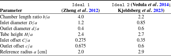


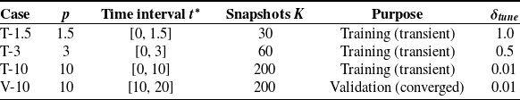


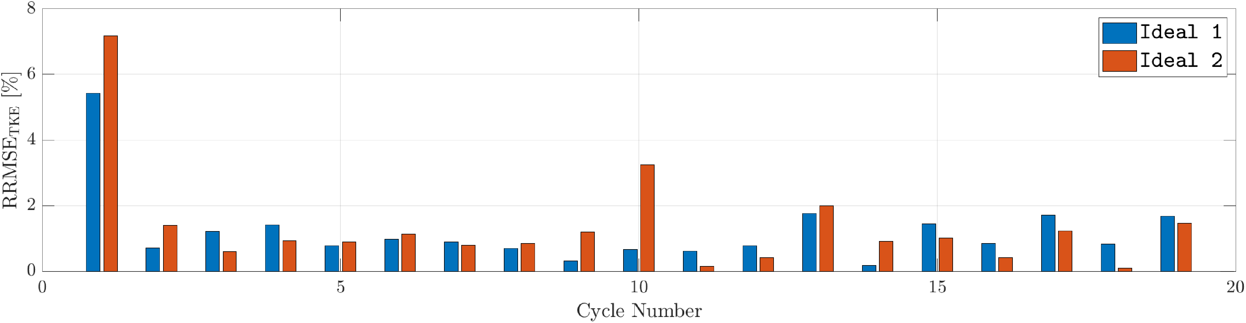
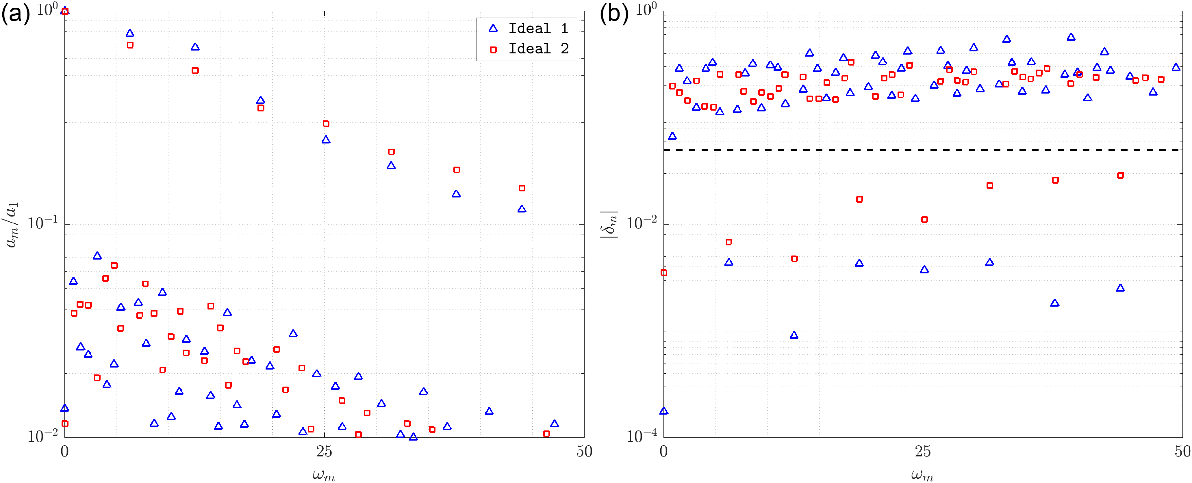


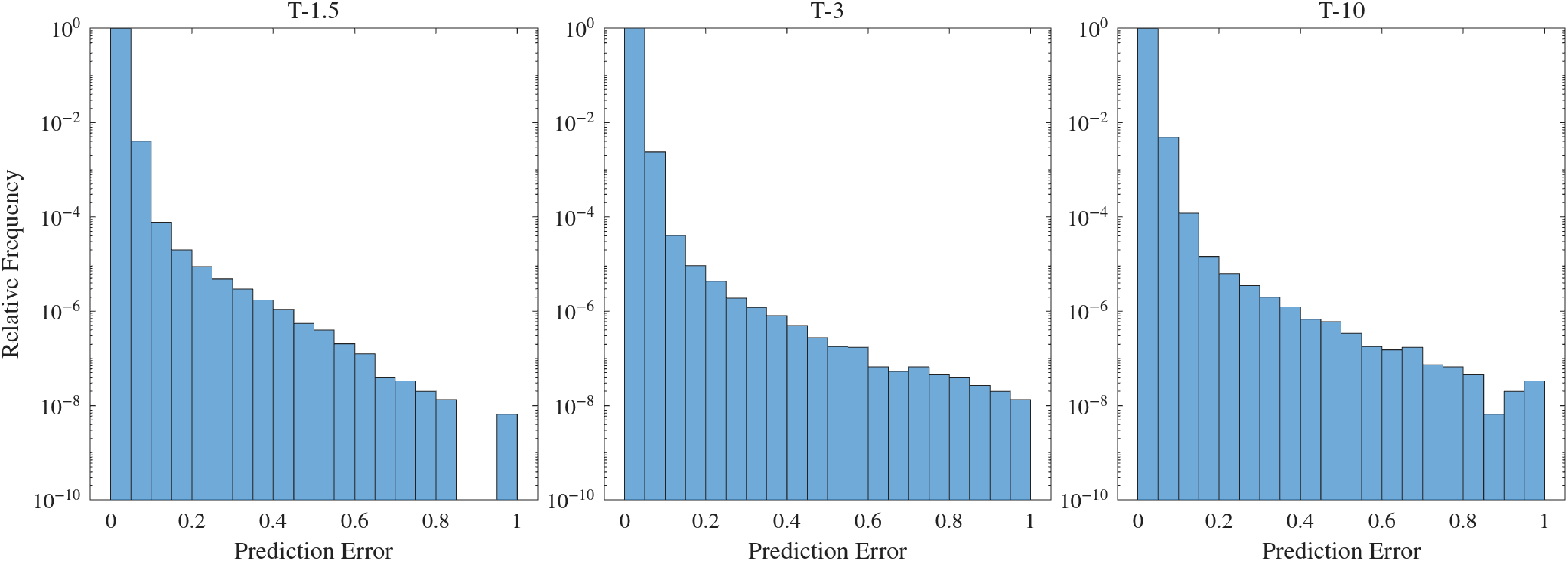

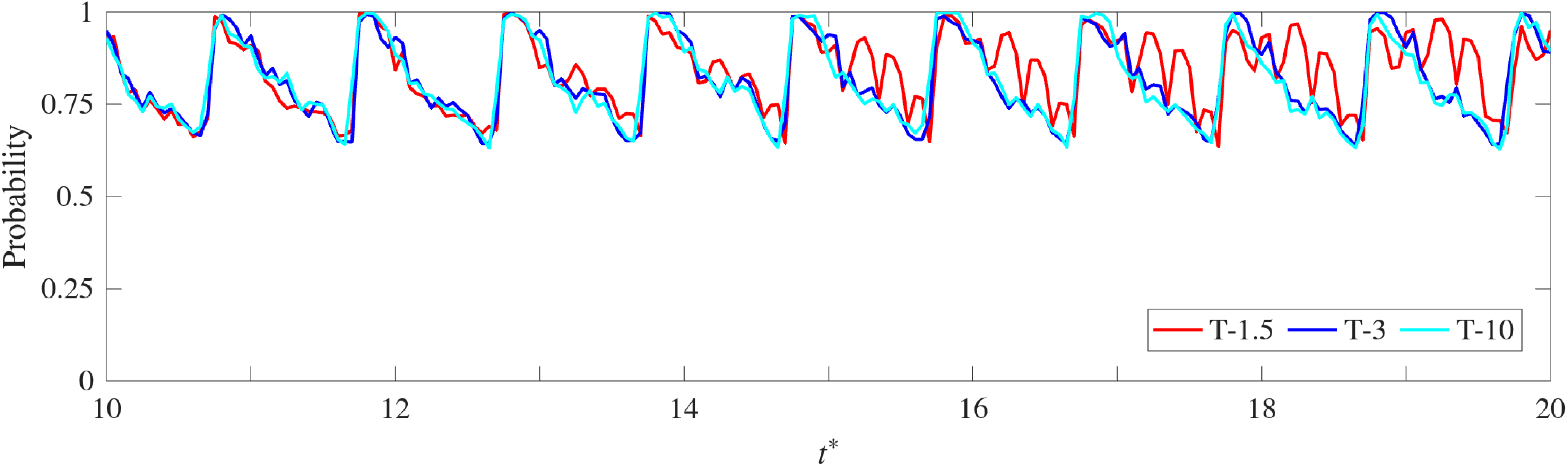


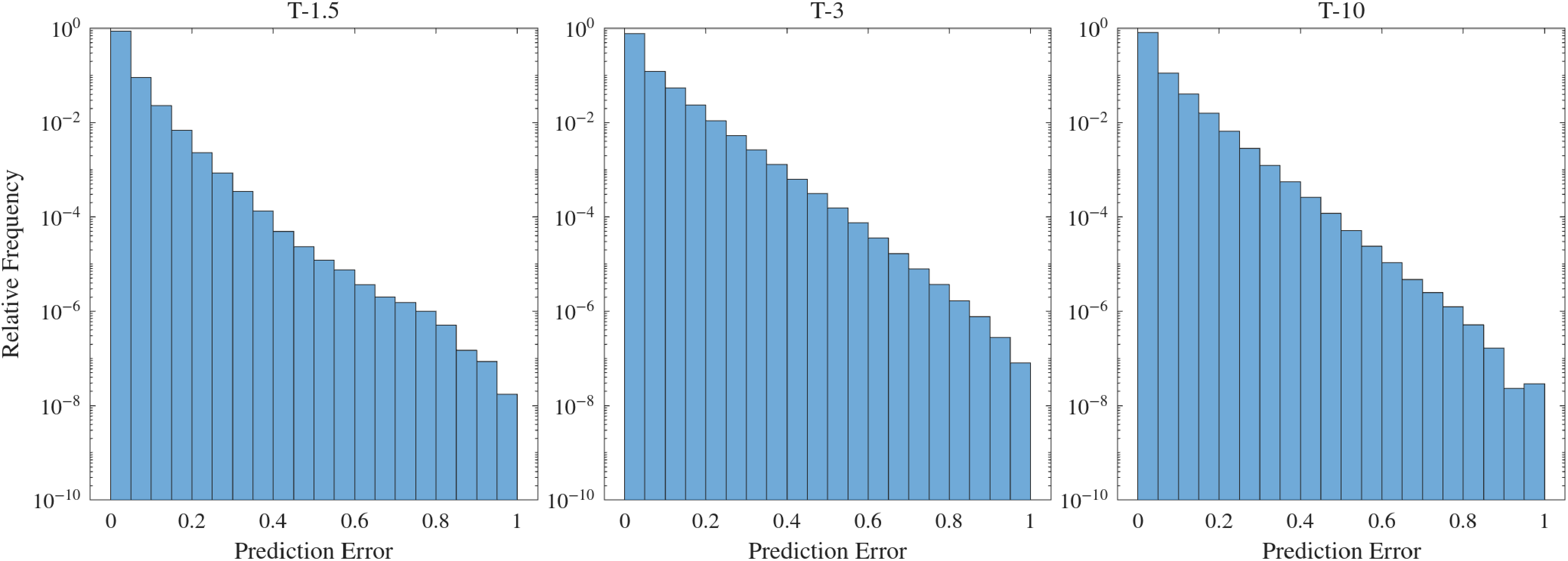

 Open access