


1. Introduction
Agriculture provides the main source of food for human consumption. Agricultural prices are directly related to the stability of national economics and the improvement in people’s living standards. China is a prominent example, having shifted from an agricultural economy to an industrial economy within four decades. Along with economic development, China’s commodity futures market has experienced rapid growth in the past three decades (Li et al., Reference Li, Chavas, Etienne and Li2017). According to the China Securities Regulatory Commission (2018), China has gradually formed a relatively complete agricultural futures trading mechanism. Driven by the advantages of large liquidity, high transparency, and low trading cost, the futures market runs much faster in responding to information flows than the spot market does. Price signals from futures markets are accordingly considered the “beacon” of spot trading and the “vane” of spot prices. The evolving futures markets in China indicate a need to better understand how they function. Better transmission effects between futures prices and spot prices have the potential to boost the price discovery function of futures markets. An important subject that has received much attention from researchers, producers, and policy makers is the dynamic linkages between futures prices and spot prices in the Chinese agricultural commodity markets. More specifically, how do price signals diffuse across the futures and spot markets? How have the transmission effects of futures and spot prices changed over time? Are there different behaviors from each market in response to external factors? Definitive answers to these questions would provide information and implications for the market participants to better understand the price discovery function in agricultural futures markets. In this article, we attempt to investigate these issues by estimating the linkages between the futures market and spot market based on the rolling window cointegration approach.
The full functioning of the futures market is closely related to vibrant spot trading; thus, efficient price transmission drives a wedge between the futures market and the spot market and exerts a critical effect on the function of the futures market, such as price discovery. The topic of the price discovery function of the futures market has drawn the interest of scholars (Adaemmer, Bohl, and Christian, Reference Adammer, Bohl and Christian2016; Gay, Simkins, and Turac, Reference Gay, Simkins and Turac2009; Yang and Leatham, Reference Yang and Leatham1999). A large body of literature examines whether the market efficiently exerts its function of price discovery function from the perspective of price transmission, especially because cointegration testing methods were successively proposed by Engle and Granger (Reference Engle and Granger1987) and Johansen (Reference Johansen1997). Under a similar framework, several measurements have been well developed and widely applied in the agricultural economics literature, such as the cointegration test, error correction model (Aulton Ennew, and Rayner, Reference Aulton, Ennew and Rayner1997; Bekiros and Diks, Reference Bekiros and Diks2008), Granger causality (Kellard et al., Reference Kellard, Newbold, Rayner and Ennew1999) at the first-order mean level, and the multiple GARCH (generalized autoregressive conditional heteroscedasticity) models (Bhar, Reference Bhar2001; Brümmer et al., Reference Brümmer, Korn, Schlüßler and Jaghdani2016; Kang, Cheong, and Yoon, Reference Kang, Cheong and Yoon2013; Zhong, Darrat, and Otero, Reference Zhong, Darrat and Otero2004) from the second-order variance perspective. There is also an argument that a large impact could notably trigger structural breaks, which would break and then rebuild the long-term relationship between variables (Peri, Baldi, and Vandone, Reference Peri, Baldi and Vandone2013). When being conscious of the potential structural breaks, many time-series models appropriate for nonstationary data have been developed, and some types of these models that are in wide use in this field are the TVECM (threshold vector error correction model; Piggott, Reference Piggott2001) and MS-AVECM (Markov-switching assymetric vector error correction model; Nemati and Saghaian, Reference Nemati and Saghaian2018). Such a threshold framework works well in generally solving nonlinear issues, but it could fail to detect cointegration in an extreme scenario where the cointegrating relationship appears only beyond the critical threshold.
The aforementioned literature provides a foundation for further study, but there appear to be certain limitations because of its static framework. The empirical findings of the previously discussed works are somehow mixed, partly because of the usage of different sample periods. Some studies support the existence of the price discovery function in certain sample periods whereas others do not. The framework of the one-off static analysis, most importantly, cannot tell us how price transmission between the futures market and its physical market is changing against exogenous shocks, such as policy adjustment. With the development of economic models, the time-varying characteristics of the spillover effect have attracted much attention in the financial futures field (Brada, Kutan, and Zhou, Reference Brada, Kutan and Zhou2002; Guidi and Ugur, Reference Guidi and Ugur2014; Mylonidis and Kollias, Reference Mylonidis and Kollias2010). Although a predominant number of empirical studies have focused on financial markets, some recent studies have extended the analysis to commodity markets as well, taking agricultural product futures markets as cases (Peri and Baldi, Reference Peri and Baldi2013; Wang, Lin, and Shih, Reference Wang, Lin and Shih2011). Adammer, Bohl, and Christian (Reference Adammer, Bohl and Christian2016) and Adammer and Bohl (Reference Adammer and Bohl2018) adopted the time-varying parameters of the Kalman filter to effectively detect the temporary effects in the process of price discovery, and they indicated that this function of the futures market takes effect when prices are soaring. These methods to obtain time-varying parameters can also track an evolving system, but they usually are sensitive to model biases and require unrealistic assumptions. The following merits of the rolling window approach can be regarded as a supplementary explanation for why we choose the research paradigm of a rolling cointegration analysis. First, the phenomenon of overgeneralization rarely occurs when information can be fully extracted from the sample data. Second, taking the multistage nature of the price discovery process into account, it roundly grasps the complete picture of the transmission effect along with time. Finally, mixed data including potential break points are replaced by data sets regenerated by rolling and iterating (Peri and Baldi, Reference Peri and Baldi2013), which could result in more comprehensive and convincing results.
To date, we know little about the price discovery function of agricultural futures markets in China from a time-varying perspective. The usefulness of a rolling cointegration analysis is applied to this dynamic progress. Taking key agricultural commodities (i.e., wheat, rice, corn, and soybeans) as cases, there are two key components included in this article. First, the static analysis of the transmission effects using the entire sample from April 2009 to May 2018 proposes that the leading role of the futures market in price transmission is applicable in Chinese agricultural futures markets. Second, we apply the rolling window approach (including 1,929 subsamples in total) to capture the time-varying characteristics of price transmission effects, with a special focus on dynamic panorama under the background of economic and policy changes. Differences in both the frequency at which cointegration appears and its duration indicate that the transmission effects between futures prices and spot prices in the corn and soybean markets are stronger than those in the wheat and rice markets. Different from the results of the normal vector error correction model (VECM), there is less support for the stable existence of a price discovery function in the agricultural commodity futures market, especially being in an uncertain economic environment. Of special interest is that in a case where oil prices rise and drop suddenly and sharply, price transmission from futures to spot prices at the same time may be weakened and even distorted, which could be attributed to price stabilization policies against unstable economics and their lagged effects. This highlights the importance of economic stability for the price discovery function of futures markets. The findings also confirm the positive effects of the market-oriented reform in the corn and soybean markets, because such reform could release market power and intensify the leading role of futures markets in pricing. We accordingly suggest promoting the duly and properly market-oriented reform of wheat and rice prices based on carefully and scientifically evaluating the potential impact of policy changes on these markets.
The rests of the article is organized as follows: We introduce the basic features of the data set in Section 2. Section 3 details the empirical model employed in the study and the technical principles of the rolling window approach. In Section 4, corresponding empirical findings under static and dynamic frameworks are presented, discussed, and interpreted, respectively. Section 5 concludes and presents ideas for further work.
2. Sample data
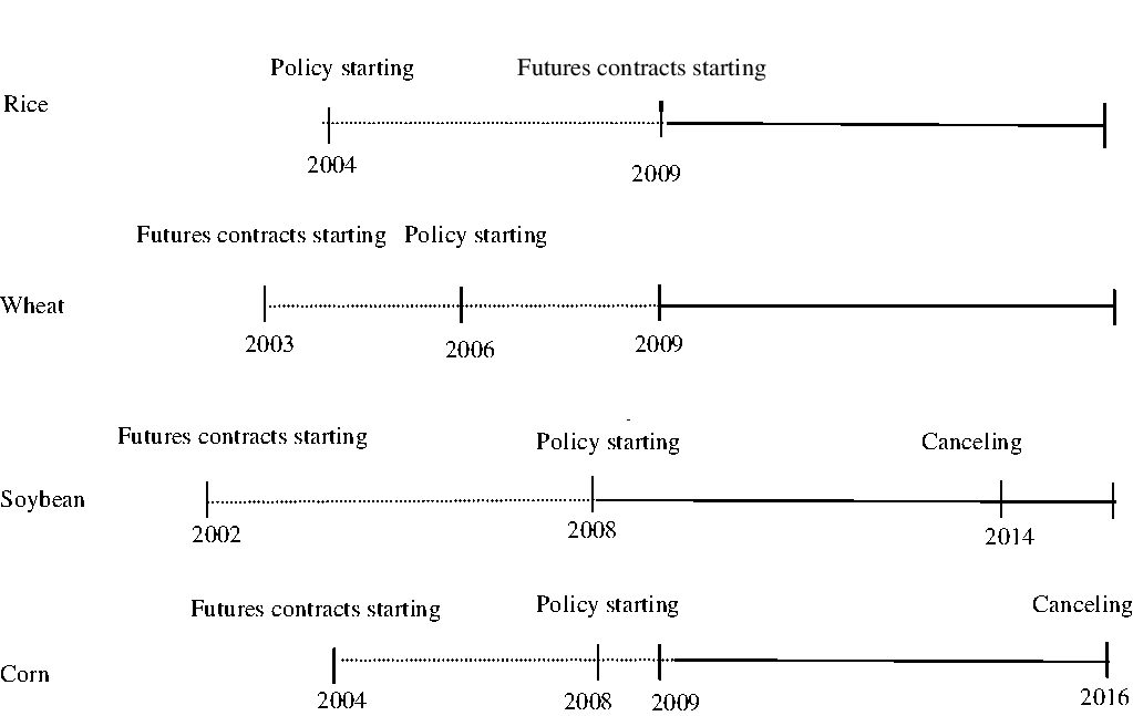
With application to Chinese corn, soybean, wheat, and rice markets, this article studies the price transmission effects between futures markets and spot markets. To ensure food security in China, there are two key programs that are influential in price stabilization: the Minimum Purchase Price policy for wheat and rice and the National Provisional Reserve (NPR) policy for corn and soybeans. Although both are price support policies, there is a divergence that exists in their implementation time, coverage scope, and control intensity (Li, Li, and Chavas, Reference Li, Li and Chavas2017). Figure 1 presents the start and end points of “policy execution” and the start time of futures contracts. Because the futures market, as an emerging market, is characterized by high growth and multiple stages, high-frequency daily data are more informative to show the dynamic evolution of the price discovery process. Considering the availability of data, this article sets up consistent periods (from April 20, 2009, to May 31, 2018) for corn, soybeans, rice, and wheat to easily make horizontal comparisons across agricultural commodity markets. After removing the days of nontrading, there are 2,160 sets of matched data in total. The daily spot prices of corn, soybeans, rice, and wheat are correspondingly estimated using the national weighted average prices, and the daily futures prices originate from the daily settlement prices of active contracts, both of which are available from the Wind database (https://www.wind.com.cn/en/data.html).
The listing time of four grain futures contracts and start and end times of the implementation of the price support policy.
Under the strategy of food security, staple grain prices are all subject to the macrocontrol of the Chinese government to different extents. They present diverse trend characteristics because of the different intensity and time of intervention. The ZA test (Zivot and Andrews, Reference Zivot and Andrews2002) traces the break point in each price series. For example, the spot prices of soybeans and corn presented structural breaks in September 2014 and August 2015, respectively. Those break points corresponded to the Chinese policy shifts regarding the soybean and corn (in trial) price support programs. There is a similar case in the wheat market—a fall in the price has appeared because of a cut in the support price since 2017. The last decade has witnessed different price trajectories in the Chinese agricultural commodity markets. As shown in Figure 2, there are price trends that vary from one market to another. Generally, wheat and rice prices increase smoothly, whereas soybean and corn prices boom and bust (i.e., climb up and then decline). An inverted V-shaped pattern in the soybean market and an inverted U-shaped pattern in the corn market are exhibited for both futures and spot prices. It often seems that spot prices follow futures prices and mimic their ups and downs, perhaps with a few lags; however, the wheat market presents different growth patterns in rising spot prices and fluctuating futures prices, as does the rice market. In Table 1, the descriptive statistics show that futures prices have higher volatility than spot prices in the soybean and corn markets, but the opposite is true in the rice and wheat markets. Jarque Bera’s statistics reject the null assumption of a normal distribution of prices in Chinese agricultural product markets. In addition, the correlation between price series is highest in the corn market, followed by soybeans, rice, and wheat in sequence.
The trends in futures and spot prices in Chinese agricultural commodity markets.

Descriptive statistics of futures and spot prices

The prices of wheat and rice have been shaped by the government’s price support policies and import quotas. Simply stated, the Chinese government will purchase surplus grain from farmers at the given prices if the market prices are below the floor; volume limits on import quotas are set annually to maintain high self-sufficiency as “strategic” crops. The combined actions of these policies play a dominant role in the wheat and rice markets, such that there appear “policy-oriented” price volatilities of wheat and rice, characterized by gentle fluctuations in price growth, which eventually lead to a vicious circle of “simultaneous increases” in production, imports, and inventory. Similarly, because of stable market expectations and narrow profit margins, there are fewer futures traders and less trading in the futures markets, which is the reason why the futures prices did not experience large volatility.
However, unlike other self-sufficiency foods, the multifunctionality of corn, such as for cereals, fodder, and energy, makes its price vulnerable to the shocks of many market forces, such as energy and its substitutes. Meanwhile, after 2016, the corn market gradually switched from policy leading to marketization pricing, which improved its sensitivity and response speed to information. The price of corn dropped significantly without minimum price support, as shown in Figure 2. The corn futures market has thereby attracted more hedgers who are interested in avoiding risk and speculators who attempt to profit from price volatility, and these have tended to strengthen the connection between the futures and spot markets since the end of 2016 (in Fig. 2). Of special note, the corn market, rather than the soybean market, has the highest correlation between futures and spot prices in the scenario in which the Chinese government has basically been deprived of its control of the soybean price because of the country’s serious import dependence (less than 25% self-sufficiency). Soybeans have been opened up most to world trade and increasingly integrated into the global financial system since being removed as a “strategic” crop. However, owing to large imports from the United States, soybean contracts on the Chicago Board of Trade (CBOT) are regarded as a preferred alternative whereby the Chinese soybean traders hedge risks. This somewhat explains why a lower correlation between the spot and futures markets in China appeared. According to the previous discussion, the different extents to which spot prices are related to futures prices across varieties could be attributed to the differences in market mechanisms shaped by policies.
3. Methodology
As a comprehensive prediction for the future status of supply and demand, the futures price is generated from open bidding and evolves in response to the information available to market participants. Participants in agricultural futures markets are composed of producers, sellers, processors, and importers-exporters, as well as speculators, the majority of which are familiar with commodity markets and able to expect future trends in prices from different perspectives. They submit ideal prices based on the available information (e.g., weather) to compete with numerous traders and contribute to forming the futures price. Overall, the futures price is an authoritative and advanced prediction for the future state according to the current information, which thereby makes it characterized by price discovery. Based on this, the price discovery function means that futures prices are unbiased estimates of future spot prices—that is, F t = E(S T |I t ), where I t represents the information set at the tth day, S T refers to the spot price at the time (Tth) of the due date, and F t is the futures price on the tth day. This proves that the futures price will generally inch toward or even become equal to the spot price with the delivery date of a futures contract approaching. In addition, there are other arguments on the relationship between the spot and futures prices. For example, the futures price is equal to the sum of the spot price and the holding cost in the pricing model of the cost of carrying; the futures price could provide the guidance for agricultural produce in turn and thus affect the spot price. These points provide theoretical support for the “price discovery function of the futures market.”
Indeed, the convergence property between futures and spot prices is consistent with the hypothesis that arbitrage binds prices into a long-run relationship (Saghaian, Reference Saghaian2010). It is now an established practice to test the price transmission across markets by cointegration analytical approaches. In this case, we adopted this mainstream research thinking, combining a cointegration relationship test with vector error correction analysis, to study the transmission effects between futures prices and spot prices. After taking the first difference, the cointegration equation can be described as
 $$\Delta {Y_t} = \alpha {\beta ^{'}}{Y_{t - 1}} + \sum\nolimits_{i = 1}^{k - 1} {{\Gamma _i}\Delta {Y_{t - i}}} + {\varepsilon _t},$$
where the rank of Π = αβ is r, which is equal to 0 or 1 in this study. The null hypothesis (H 0: r = 0) denies the existence of a cointegration relationship between the futures price and the spot price because of a nonstationary linear combination between sequences. Under the alternative hypothesis (H 1: r = /0), there appears a smooth linear combination between the two series. Empirically, the trace test function in equation (2) plays a decisive role in whether or not to accept the null hypothesis and accordingly judge the existence of a significant cointegration relationship.
The overall judgment of whether the equilibrium relationship exists can be drawn by comparing the trace statistic λ trace with its critical value. Other indictors in equation (2) to measure λ trace are the observation value of T, the ith maximum eigenvalue λ i of the constraint matrix Π, the number of variables n, and the rank r of the constraint matrix.
 $${\lambda _{trace}} = - T\sum\nolimits_{i = r + 1}^n {ln(1 - {\lambda _i}),r = 0,1, \ldots ,n - 1} .$$
According to the analysis theory of the Johansen cointegration test, the series are indeed cointegrated once a smooth linear combination appears among them, although the individual series itself could be nonstationary. In the case of a known long-term equilibrium relationship, the VECM could be further established to estimate short-run speeds at which one series converges dynamically to a long-run relationship with the other. Theoretical analyses indicate that futures and spot prices connect directly with each other. Based on that, with a focus on long-term equilibrium and short-term adjustment between spot and futures prices, it is reasonable to include only them in the VECM. The equation of the VECM is denoted as follows:
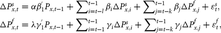 $$ \Delta P_{x,t}^s = \alpha \beta _1^{'}{P_{x,t - 1}} + \sum\nolimits_{i = t - l}^{t - 1} {{\beta _i}\Delta P_{x,i}^s} + \sum\nolimits_{j = t - k}^{t - 1} {{\beta _j}\Delta P_{x,j}^f} + \varepsilon _t^s, \\\Delta P_{x,t}^f = \lambda \gamma _1^{'}{P_{x,t - 1}} + \sum\nolimits_{i = t - 1}^{t - 1} {{\gamma _i}\Delta P_{x,i}^s} + \sum\nolimits_{j = t - k}^{t - 1} {{\gamma _j}\Delta P_{x,j}^f} + \varepsilon _t^f,$$
where ε
t
is an error term, and l and k represent the optimal time lags determined by the minimal values of final prediction error (FPE), Akaike information criterion (AIC), likelihood radio (LR), Schwarz criterion (SC), and Hannan Quinn (HQ). Aggregative variables, $\Delta P_{x,t}^s$
and
$\Delta P_{x,t}^s$
and $\Delta P_{x,t}^f,$
are the first differences in prices, of which the subscript x is set to “b,” “c,” “r,” and “w,” representing “soybeans,” “corn,” “rice,” and “wheat,” respectively. The s and f of their superscripts correspond successively to the spot price and the futures price.
$\Delta P_{x,t}^f,$
are the first differences in prices, of which the subscript x is set to “b,” “c,” “r,” and “w,” representing “soybeans,” “corn,” “rice,” and “wheat,” respectively. The s and f of their superscripts correspond successively to the spot price and the futures price.
The aforementioned VECM measures the price transmission effect via three types of parameters. The first type includes error correction coefficients, denoted by α and λ, the relative speed that (how fast) the spot price and the futures price could rebuild the long-term cointegration status, after the markets are shocked by external factors, such as policy and technology changes. If α is significant but λ not, this means that the spot price is the one and only dynamic factor in the process of recovering to the equilibrium between two variables, and accordingly, the price is transmitted from the futures market to the spot market. In contrast, we can infer that there is significant transmission from the spot price to the futures price. When both are significant, the market with a large absolute value of the error correction coefficient is subject to correct toward the equilibrium faster following short-term shock; thus, we deduce that the other market performs better in price discovery. The second type of parameters are cointegration coefficients—namely, β
1 and γ1—which reflect the direct long-term relationship between prices. They are used to measure the degree to which the spot (futures) price is affected by futures (spot) price changes. The first-lagged error correction terms are expressed by $\beta _1^{'}{P_{x,t - 1}}$
and
$\beta _1^{'}{P_{x,t - 1}}$
and $\gamma _1^{'}{P_{x,t - 1}},$
which refer to the departures from the long-term relationship after external shocks. The last type of parameters are interaction coefficients, β
j
and γ
i
, reflecting the short-term mutual effects between prices. If β
j
(γ
i
) is significant, this means that the futures (spot) price will affect the spot (futures) price in the short term. Taken together, the three kinds of coefficients are complementary, providing handy tool kits for analyzing the transmission effects between futures prices and spot prices.
$\gamma _1^{'}{P_{x,t - 1}},$
which refer to the departures from the long-term relationship after external shocks. The last type of parameters are interaction coefficients, β
j
and γ
i
, reflecting the short-term mutual effects between prices. If β
j
(γ
i
) is significant, this means that the futures (spot) price will affect the spot (futures) price in the short term. Taken together, the three kinds of coefficients are complementary, providing handy tool kits for analyzing the transmission effects between futures prices and spot prices.
As mentioned previously, empirical analyses based on the whole time span can only reflect the general relationships between futures prices and spot prices and cannot track the dynamic changes in the relationships, which may lead to overgeneralization and even biased estimations. The dynamic rolling window cointegration test is an alternative form of the static cointegration test. It is more informative and refined for the reason that it captures the dynamics changes in the cointegration relationship over time. It makes no more assumptions than the ordinary cointegration tests, but it has more requirements for the data. Dynamic rolling window tests do need more observations than the static cointegration test to validate the detection in each period. As shown subsequently, we made efforts to collect the 10-year daily futures-spot prices in four Chinese key agricultural markets, which is informative enough for us to form the dynamic rolling windows in this research. Hence, cointegration analysis extended and modified by the rolling window approach is a statistical technique used to explore the changes in interactive patterns or relationships over time. Under the analysis framework of the Johansen cointegration equation and the VECM, the rolling window approach to structure subsample intervals captures dynamic transmission effects of futures prices and spot prices in each subsample. Figure 3 introduces the operation procedures of the rolling window approach. Under the fixed window length, each scroll forward generates a new subsequence by adding a new datum at the end of the previous window and removing the first datum.
Schematic diagram of the rolling window principle: (a) General cointegration analysis with the fixed time window. (b) Rolling cointegration analysis with rolling time window.
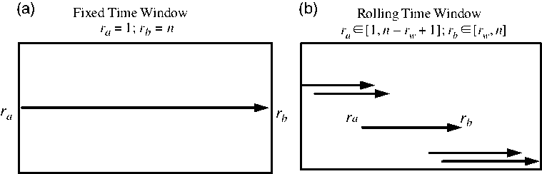
Let n be the total number of samples, equal to 2,160 in this study. Denote r a and r b as the starting and ending fractions of the subsample, respectively, and r w as the fixed window size. Then, we have r w = r b − r a + 1; r a moves forward 1 unit every time, and so does r b . After rolling, n – r w + 1 pairs of price subsequences can be obtained altogether. With the fixed window, the trace statistics and coefficients in the VECM are calculated by varying the starting point r a from 1 to n – r w + 1 and varying the end point r b from r w to n. the Johansen cointegration test and the VECM based on rolling window approach are shown as in equations (4) and (5), respectively:
 $${\lambda _{trace,[ra,rb]}} = - {T_{rw}}\sum\nolimits_{i = r + 1}^n {ln(1 - {\lambda _{i,[ra,rb]}})} ,r = 0,1, \ldots ,n - 1,$$
 $$\eqalign{\Delta P_{x,t}^s = {\alpha _{[ra,rb]}}\beta _{1,[ra,rb]}^{'}{P_{x,t - 1}} + \sum\nolimits_{i = t - 1}^{t - 1} {{\beta _{i,[ra,rb]}}\Delta P_{x,i}^s} + \sum\nolimits_{j = t - k}^{t - 1} {{\beta _{j,[ra,rb]}}\Delta P_{x,j}^f} + \varepsilon _t^s \cr \\\Delta P_{x,t}^f = {\lambda _{[ra,rb]}}\gamma _{1,[ra,rb]}^{'}{P_{x,t - 1}} + \sum\nolimits_{i = t - 1}^{t - 1} {{\gamma _{i,[ra,rb]}}\Delta P_{x,i}^s} + \sum\nolimits_{j = t - k}^{t - 1} {{\gamma _{j,[ra,rb]}}\Delta P_{x,j}^f} + \varepsilon _t^f,}$$
where starting point (r a ) and ending point (r b ) of the window are put on r a ϵ [1, n – r w + 1] and r b ϵ[r w ,n]; the sample size for each test is equal to the fixed window size, namely, T rw = r w ; εt is an i.i.d. (independent and identically distributed) error term—that is, ε t ∼ i. i. d. N(0, σ [ra,rb] 2). The Johansen cointegration test and the VECM are conducted successively in new subsequences, denoted as [r a ,r b ], for each group to obtain the time series of the trace statistics, cointegration coefficients, and error correction coefficients.
4. Result analysis
4.1. Static test of transmission effect between futures prices and spot prices
A unit root test should be performed to explore whether the futures price and spot price are stationary before the cointegration test is carried out. In Table 2, the results of augmented Dickey-Fuller (ADF) tests and augmented Dickey-Fuller generalized least squares (ADF-GLS) show that the original price series are nonstationary, but their first-difference sequences are stationary—namely, I (1)—which satisfies the premise of the cointegration test and the VECM. Johansen cointegration tests for all varieties provide the evidence of the long-term equilibrium between futures prices and spot prices at the 5% significance level. Given that the cointegration relationship exists, the VECM is further used to quantitatively evaluate the retro-regulation mechanism of each market, as shown in Table 3. The error correction coefficients of spot prices are all negative and significant at the 1% level, indicating that the spot prices of corn, soybeans, wheat, and rice can return to the long-term equilibrium by the traction of counterforce after being shocked by external factors. Similarly, it is found that the futures price is also somewhat corrected toward original equilibrium in the corn market, whereas in the soybean, rice, and wheat markets, the recovery to long-term equilibrium is mainly achieved through the adjustment of spot prices. By comparing the relative size of the absolute values, it turns out that the deviation of spot prices could be adjusted at a faster speed in the corn market.
The results of unit root and Johansen cointegration

Notes: Asterisks (*** and **) correspond to 1% and 5% significance level, respectively. ADF, augmented Dickey-Fuller; ADF-GLS, augmented Dickey-Fuller generalized least squares.
The results of vector error correction model estimation

Notes: The values in brackets are the t-statistics; the optimal lag order of the Johansen cointegration test is “2,” determined by minimal values of final prediction error (FPE), Akaike information criterion (AIC), likelihood radio (LR), Schwarz criterion (SC), and Hannan Quinn (HQ).
It is worth clarifying that, regardless of whether there is a change in policy type in the corn and soybean markets or a change in support strength in the wheat and rice markets, different policies have been implemented over time, which causes the role of the market in pricing to change greatly. Despite the effectiveness of the ZA test in detecting the break point of each series, it does not identify the break points of the relationship between two variables. The method of Bai and Perron (Reference Bai and Perron2003) will be used to perform the simultaneous estimation of multiple break points in the VECM, by testing or assessing deviations from stability in statistical relation. The results of multiple structural break points in the transmission effects between futures and spot prices are reported in Table 4. Based on the detected break points, there are significant impacts of energy shocks in 2014 and impacts of policy reforms in 2014 and/or 2015 on the soybean and corn markets. In addition, the structural break points detected are greatest in the rice market and least in the wheat market. In 2011, because of an increase in support prices and the frequent phenomenon of “panic buying,” the spot prices of the wheat and rice markets were high, but the futures market suffered, the prices of which were falling. These factors worked together and led to the break point of 2011 in the wheat and rice markets. An economic relationship varies on the two sides of any break point, so the results of one-off whole samples to conclude the existence of a “price discovery process” in these markets is less reasonable. Moreover, the soybean and corn markets were jointly shocked in the years 2014 and 2015. We conjecture that the change in this relationship was because of policy changes. An in-depth analysis of specific shocks on the price discovery process would be warranted by further rolling time window analysis.
The results of the test for multiple structural changes

Notes: Assume that there are m break points that are boundaries of alternating regimes (m + 1). The optimal number of break points could be determined by the minimum Bayesian information criterion (BIC) estimator, and the dates of the break points can be traced. RSS, residual sum of squares.
4.2. Dynastic characteristics of transmission effect between futures prices and spot prices
This section uses the rolling window approach to further test and analyze the cointegration relationship and error correction between futures and spot prices. Consider that cointegration is a long-run property, and the presence of cointegrating relations can be captured only under the requirement of long time spans. However, a longer window tends to hide partial information on time-varying effects and yield smoother rolling window estimates than shorter ones. Based on both considerations, the size of the rolling windows is set to 232 days (i.e., approximately one financial year; Mylonidis and Kollias, Reference Mylonidis and Kollias2010; Peri and Baldi, Reference Peri and Baldi2013), of which the optimal lag orders are determined by AIC and SC. After rolling forward and performing an empirical test for each subsequence, we obtain three indicator series—trace statistics, cointegration coefficients, and error correction coefficients—for a total of 1,929 sets.
4.2.1. The rolling cointegration relationship
As previously mentioned, whether or not a cointegration relationship exists depends directly on the significance of the trace statistics. To achieve a visualized comparison, the trace statistics in this study are standardized (i.e., the trace statistics are divided by the 5% critical value). If the standard values in the subintervals are not lower than 1, we will reject the null hypothesis at the 5% significance level and support the existence of a cointegration relationship. According to the statistical results of the normalized trace statistics in Table 5, the maximum values are all greater than 1, indicating that specific subintervals, where futures prices and spot prices cointegrate with each other, are supposed to exist. In terms of the mean and the median, the normalized trace statistics are greater than 1 in the corn market, followed by the soybean market. This result supports the existence of a stable and strong correlation between the futures price and the spot price in the two markets. However, the normalized trace statistics of both wheat and rice are much lower. Weaker cointegration relationships mean that the spot and futures markets are in relative isolation.
The normalized trace statistic of the rolling Johansen cointegration test

The statistical probability of cointegration between futures prices and spot prices of four agricultural products ranges from 17.63% to 55.46%. The highest frequency (more than 50%) of cointegration relationships appears in the corn market, and the frequency in the soybean market ranks second, with a little more than 30%. There is an approximately 20% probability for “≥1 ratio” in the wheat market, followed by the rice market, which further demonstrates that their futures prices and spot prices are loosely linked with one another. The path to reform the market mechanisms, designed according to national conditions, varies greatly across agricultural product markets. Taking soybeans and corn as pioneers, China has started the marketization reform of main grains since 2014, which has gradually cancelled the country’s NPR policies and launched the target price and marketization purchase policies. Under the background of “depoliticization” in the corn and soybean markets, spot prices can respond sensitively to market signals, especially to the information flows from futures markets. In contrast, the role of government in pricing tends to overshadow the role of the market itself, which contributes to forming a fragmented state across spot and futures markets. Even if the subsidy level for wheat and rice has been reduced gradually, it still has a distorting effect on the markets. Thus, the level of cointegration between futures prices and spot prices varies among different grain markets, and a stable and long-term cointegration relationship between futures prices and spot prices has not been formed overall in the Chinese agricultural product market.
Figure 4 is the dynamic graph of the normalized trace statistics drawn on a unified timeline. Generally, each group of trace statistics changes obviously with time, detecting the unstable equilibrium and time-varying relationship between futures prices and spot prices. The cointegration relationship appears yearly in the corn market and shows the characteristics of short cycles and high frequency. Taking 2015 as the watershed, the cointegration relationship was relatively stable and concentrated before 2015, and then it changed frequently. The soybean market almost shared the peak and trough of the trace statistics at roughly the same time as the corn market, but its significant cointegration relationships would be for a relatively shorter time. Nevertheless, the distribution of cointegration relationships characterized by shorter periods and lower frequencies in the wheat and rice markets is dispersed. A cut in their support prices since 2017 has contributed to highlighting the role of the market itself.
Time-varying tendency of rolling trace statistics.

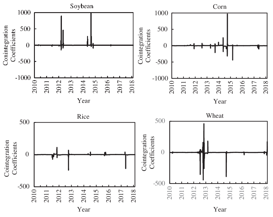
The rolling cointegration coefficients reflect the extent to which futures prices exert an influence on spot prices within a specific sample interval. The high sensitivity of futures markets to market environments leads to abnormal values of rolling cointegration coefficients when the markets encounter a large shock. Based on this, the rolling cointegration coefficients are extracted and spread along the time axis to detect the time points when unexpected impacts appear. As shown in Figure 5, several abnormal values of rolling cointegration coefficients occur, most of which are involved in the neighboring areas of the break points shown in Table 4. For example, the cointegration coefficients in the soybean market peaked at 3,515.65 in a rolling sample interval of 2014, and in the corn market, they successively reached a maximum of 969.98 and a minimum of −437.51 in 2015. We attribute these values to the shocks brought by energy market turbulence in 2014 and the strategic shift in price policy for soybeans (in 2014) and corn (in 2015). Similarly, with the guidelines of promoting supply-side structural reform and deepening the formation mechanism of agricultural prices proposed by the “No. 1 central document” of the Chinese government in 2017 (http://www.chinadaily.com.cn/china/2017-02/05/content_28108022.htm [accessed February 5, 2017]), a series of policies targeted at rice and wheat have changed, such as a cut in purchasing prices. Additionally, in the scenario when international oil prices boomed and then collapsed from 2012 to 2014, abnormal values of the cointegration coefficients also appeared frequently across agricultural products in China. It has been proved that changes in energy prices affect food markets (Saghaian et al., Reference Saghaian, Nemati, Walters and Chen2018; Xiarchos and Burnett, Reference Xiarchos and Burnett2018).
Time-varying tendency of cointegration vectors.
4.2.2. The rolling effects of price transmission effect
Rolling out correction coefficients along the timeline is conductive to tracing the dynamic effects and then further determining how price transmission may be affected in a neighborhood of the event. The temporary deviation caused by short-term shocks tends to be pulled back by a long-term equilibrium state, and accordingly, we pay more attention to the scenario in which the cointegration relationships are significant. The error correction coefficients in Figures 6 and 7 indicate how quickly the spot price and the futures price return to their long-run equilibrium, respectively, after a temporary shock. When the rolling error correction coefficients in the spot market (Fig. 6) exceed the 95% confidence interval, the null hypothesis (H 0: α = 0) is rejected, indicating that the spot price can be continuously adjusted to reach a new equilibrium and that a reverse correction mechanism exists in the spot market within a specific subinterval. Otherwise, the null hypothesis (H 0: α = 0) is accepted at the 95% significance level. Similarly, whether an error correction mechanism exists in the futures market (Fig. 7) could be worked out through the parallel rules.
The time-varying characteristics of the transmission effect of futures prices on spot prices.
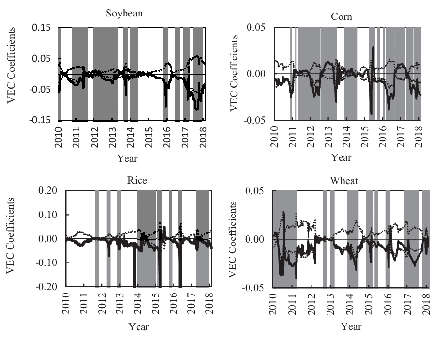
The time-varying characteristics of the transmission effect of spot prices on futures prices.

In Figure 6, the error correction coefficients of spot prices in scenarios with significant cointegration relationships are basically negative and significant throughout the rolling sample intervals. Overall, because of low cointegration levels between futures prices and spot prices in the wheat and rice markets, the error correction coefficients of spot prices are rarely significant. It turns out that the reverse correction mechanism does not function as well in the wheat and rice markets as in the other two markets. The correction speed of spot prices toward equilibrium could be reflected by the relative magnitude of the absolute error correction coefficients. Excluding some special values, the ranges of the error correction coefficients in the soybean and rice markets are relatively larger than those in the corn and wheat markets, with absolute values ranging from 0 to 0.10 for the former and ranging from 0 to 0.05 for the latter two markets.
The absolute error correction coefficients of soybeans increased sharply and reached 0.06 at the beginning of 2014, which supports the importance of cancelling soybeans’ NPR policy for boosting the price discovery function of its futures market. Although policy reform released market forces, its effect is limited because of the long-term dependence on imports and high import volume, which can be attested by the subsequent movement of the error correction coefficients. The error correction coefficients in the corn market changed from positive to negative by the end of 2015, and the absolute value increased. This indicates that the reform of the price support policy of corn accelerated the marketization process of the corn industry and strengthened the guiding role of its futures price to some degree. A set of agricultural policy reforms (i.e., adjusting and reducing the protective price of wheat and rice included) since 2017 have strengthened the linkage between futures markets and spot markets. Coincidently, the adjustment of spot prices to the long-term equilibrium has accelerated since then, likely because the role in pricing shifted slightly from the government to markets. Overall, in the scenarios when international crude oil prices were soaring (the end of 2011 to the beginning of 2012) and plunging (the end of 2014 to the beginning of 2015), the absolute error correction coefficients of the spot price in four agricultural commodity markets were close to zero and of no significance. The control policies against them seem to be the reason for the insignificant price discovery function of futures markets because these could make food prices less sensitive to outer shocks.
After rectification and standardization in recent years, the futures markets of corn and soybeans have achieved better docking with the spot market, which contributes to improving its price discovery function. From the perspective of futures market turnover, the monthly trading volume of No. 1 soybean futures contracts is relatively stable, basically maintaining between 40 million and 50 million metric tons. Recently, the activeness of the soybean futures market in China has been surpassed by the corn futures market because of the shunting effect of CBOT soybean futures trading and the rapid expansion of the corn futures market. The volume of corn contracts increased from 24.14 million metric tons in April 2009 to 56.95 million metric tons in May 2018, an increase of 135.90%. Because of the policy adjustment of corn starting in 2015, the corn futures market has been unprecedentedly active, and its trading volume has been continuously rising. In contrast, it has been proved that there is less participation in the other two futures markets, because of the thin trading volumes of futures contracts, with an average of 695,100 for wheat and 6,422,000 for rice monthly. The possible reason for the aforementioned data is that the spot prices of wheat and rice have been shaped by agricultural support policies, and the utility value of futures markets is largely compressed under stable market expectations. Specifically, a large national capacity to release or augment stocks when prices extensively soar or fall can effectively reduce speculative behavior in the wheat and rice futures markets.
Figure 7 shows that there are significant differences in the error correction coefficients of futures prices across the four agricultural products in the rolling sample intervals. The error correction coefficients of soybean, wheat, and rice futures prices are basically positive, whereas the coefficients in the corn futures market are mostly negative. This proves that a reverse error correction mechanism still exists in the corn futures market, whereas soybean, wheat, and rice futures prices tend to deviate further from long-term equilibrium after short-term shocks. In the scenarios of unstable international oil markets, the error correction coefficients of agricultural commodity futures prices had a trend of changing from positive to negative, thereby indicating that the transmission effects between spot prices and futures prices could be affected, albeit not powerfully. The error correction coefficients of futures prices in the rice market have become significant and have increased since 2017. This indicates that the reform of lowering the rice purchasing price has affected, to some extent, the function of its futures market to perceive and transmit price signals.
By comparing the spot error correction coefficients with the futures error correction coefficients, the price discovery process can be further quantified by the relative speed at which two markets adjust to the long-term equilibrium. Comparing Figures 6 and 7, with a special focus on the scenarios when the cointegration relationship is significant, it can be seen that, overall, the error correction coefficients of futures prices fluctuate greatly but are basically insignificant. This means that the futures market has a lower dependence on the cointegration relationship and seldom corrects to the long-term equilibrium on its own initiative following short-term shocks. In contrast, the spot price of agricultural products tends to correct continuously and converge to the long-term equilibrium. That is, the price signals of agricultural products are mainly transmitted along the single direction of “futures to spot,” and the agricultural product futures market occupies the main position in the process of price discovery.
5. Conclusions
Based on the daily data of futures and spot prices in the corn, soybean, wheat, and rice markets from April 2009 to May 2018, this study empirically analyzes the price discovery function of Chinese agricultural futures markets and its evolutionary process by examining the transmission effects of futures prices on spot prices. The Johansen cointegration equation and VECM are first applied to conduct a full-sample analysis of the transmission between futures prices and spot prices. The results confirm the existence of a cointegration relationship and error correction in four markets, and among them, the corn futures market runs most effectively and interacts well with its spot market. However, the existence of break points in price transmission highlights a need to better understand the dynamic change in the price discovery function, such as when futures markets function well and when they do not.
The rolling window approach is subsequently used to trace the evolution of transmission effects and to further explore the time-varying characteristics of the price discovery function. In summary, the transmission effects between futures prices and spot prices of agricultural products are affected not only by market mechanisms that are specific to each variety but also by changes in the macromarket environment, such as economic background and policy changes. Our findings provide useful insights into the factors contributing to differences in the price discovery function across commodity futures markets and to their evolution over time. The detailed results are threefold.
First, across the rolling sample periods, higher cointegration levels between futures prices and spot prices in the corn and soybean markets, characterized by a long cycle and high frequency, are derived from the tight linkage between futures prices and spot prices. For the wheat and rice markets, the cointegration relationship with the characteristics of a short period and low frequency between futures prices and spot prices testifies that they are not easily affected by each other and are almost in a state of segmentation. Therefore, when the crisis occurs, in accordance with the principle of “hierarchical monitoring,” a special focus should be placed on active futures markets (i.e., corn and soybeans). These identify the one-sidedness of all-sample analysis, because it does not identify the differences in the extent of price transmission from each market like rolling cointegration analysis.
Second, in the scenarios when cointegration relationships are significant, the error correction coefficients of spot prices are basically negative and significant throughout the rolling sample intervals, while the futures error correction coefficients are larger but less significant. This finding provides evidence that the long-term equilibrium between futures and spot markets is mainly realized through the adjustment of spot prices after short-term shocks. To be brief, the volatilities of agricultural product prices are mainly transmitted along the direction of “futures to spot,” as discussed in previous literature (e.g., Wang, Lin, and Shih, Reference Wang, Lin and Shih2011; Yang and Leatham, Reference Yang and Leatham1999) that supports the leading role the futures markets play in price discovery. Note that although the direction of price transmission has no significant differences, its strength varies across agricultural product markets. Although low-liquidity futures markets (i.e., wheat and rice) cannot fully demonstrate their functions of price discovery because of narrow investment space, high-liquidity futures markets (i.e., corn and soybeans) are sensitive to information flows and are thereby considered as price signal sources of spot trading.
Third, the transmission effects between futures prices and spot prices are easily affected by the policy environment. The market-oriented reforms of the soybean and corn prices began in 2014 and in 2016, respectively, and have, to some extent, boosted the price discovery function of the futures market, especially in the corn market. With the marketization of spot prices advancing and the liquidity pools of futures markets deepening, the price leading role of agricultural futures markets has been continuously strengthened since 2017. Additionally, the instability of the external economy, such as oil turmoil, will somewhat affect futures markets, which could be embodied in the frequent occurrences of abnormal values of the cointegration coefficients. In these scenarios, the price stability policy against volatile markets, which acts like a shield between futures markets and spot markets, tends to reduce the transmission effects and weaken the price discovery function of agricultural commodity futures markets. These findings seem to be missing in the previous literature partially because of the methodological limitations.
Based on the aforementioned conclusions, our research provides useful information about the contributing factors that affect the price discovery function in agricultural futures markets. It has explicit implications for the design and implementation of agricultural policy in China. A new and dynamic perspective to study the price discovery function of the agricultural futures market is documented as well. Most importantly, this perspective encourages researchers to explain why transmission effects between futures markets and spot markets vary over time, with a special focus on the impacts of varied macroeconomic and policy circumstances. Needless to say, the analysis presented in this article also has some limitations, and more remains to be done in such a field—which is faced with the complexity of the price discovery process and the technical requirements of targeted models. The seasonality factors, structural breaks in futures price volatility, and nonlinear dynamics have not been taken into account in the current study. These points seem to be good topics for future research in order to provide more comprehensive insights on the price discovery function of the agricultural futures market.
Author ORCIDs
Yuanyuan Xu, 0000-0002-1594-4835; Fanghui Pan, 0000-0001-8104-1549
Financial support
This work was supported by the National Natural Science Foundation of China (Grant Nos. 71673103 and 71803058) and Fundamental Research Funds from the Central Universities of China (Grant No. 2662017QD023).


 Open access