


1. Introduction
As a result of global climate warming, glaciers and ice caps are projected to shrink and retreat in all regions on Earth, continuing on the current trajectory of large-scale ice loss (Oppenheimer and others, Reference Oppenheimer2019; Rounce and others, Reference Rounce2023). Any assessment of ensuing consequences is dependent on knowledge of the ice volume existing today. This concerns not only projections of sea-level rise, but also water management in general where the regional ice volume can be a key determinant for the future availability of water for basic needs and irrigation (e.g. in the Himalaya; Pritchard, Reference Pritchard2019), or for hydro-power production, as in Scandinavia (Ekblom Johansson and others, Reference Ekblom Johansson, Bakke, Støren, Gillespie and Laumann2022). Besides total ice volume, knowledge of the spatial distribution of ice within a region, between different glaciers and within one glacier is crucial. Such maps of ice thickness and, thereby, subglacial topography are essential for future projections of glacier response to climate warming as the bed shape controls the future hypsometric distribution of ice, and through that, whether a glacier will be able to stabilize at higher elevations (Rounce and others, Reference Rounce2023). For marine-terminating glaciers, subglacial topography is crucial in determining the dynamical response to an external signal, and consequently, whether stabilization (e.g. on pinning points or bathymetric highs) or retreat of the grounding line (e.g. due to inland sloping beds) is likely to occur (Åkesson and others, Reference Åkesson, Nisancioglu and Nick2018; Frank and others, Reference Frank, Åkesson, de Fleurian, Morlighem and Nisancioglu2022). The location of future lakes and the routing of future rivers can likewise be deduced from the shape of the glacier bed (Farinotti and others, Reference Farinotti, Round, Huss, Compagno and Zekollari2019; Ekblom Johansson and others, Reference Ekblom Johansson, Bakke, Støren, Gillespie and Laumann2022). Furthermore, ice thickness maps can help both the tourism industry and scientists on fieldwork to plan economic or scientific investments (Marr and others, Reference Marr, Winkler and Löffler2022). Importantly, knowledge of subglacial topography also helps to assess the risks associated with future deglaciated landscapes, e.g. the potential for glacier lake outburst floods or landslides (Liestøl, Reference Liestøl1956; Engeset and others, Reference Engeset, Schuler and Jackson2005; Breien and others, Reference Breien, De Blasio, Elverhøi and Høeg2008; Jackson and Ragulina, Reference Jackson and Ragulina2014). Finally, the topography of future exposed lands is important in shaping the emerging habitats that form when glaciers retreat (Bosson and others, Reference Bosson2023).
To estimate ice volume and bed shape while overcoming the lack of ice thickness observations for most glaciers in the world (GlaThiDa Consortium, 2020; Welty and others, Reference Welty2020) inversion techniques have been developed that allow the derivation of subglacial topography based on surface observations. The recent years have seen continued progress in this field (Farinotti and others, Reference Farinotti2017, Reference Farinotti2021), expanding from early works on volume–area scaling (Bahr and others, Reference Bahr, Meier and Peckham1997, Reference Bahr, Pfeffer and Kaser2014) to techniques such as shear-stress-based approaches (e.g. Nye, Reference Nye1952; Linsbauer and others, Reference Linsbauer, Paul, Hoelzle, Frey, Haeberli, Purves, Gruber, Straumann and Hengl2009; Frey and others, Reference Frey2014) and mass-conservation approaches (e.g. Farinotti and others, Reference Farinotti, Huss, Bauder, Funk and Truffer2009; Huss and Farinotti, Reference Huss and Farinotti2012). With the advent of high-quality remote-sensing products regional-scale ice flow velocity-based approaches have become possible (e.g. Gantayat and others, Reference Gantayat, Kulkarni and Srinivasan2014; Millan and others, Reference Millan, Mouginot, Rabatel and Morlighem2022) alongside methods involving full ice dynamics models on distributed grids that require a combination of several observational datasets (e.g. ice velocity fields, dh/dt) and/or auxiliary model products (e.g. from a mass-balance model) as inputs (van Pelt and others, Reference van Pelt2013; Jouvet, Reference Jouvet2023; Frank and others, Reference Frank, van Pelt and Kohler2023).
While some ice volume estimates for Scandinavia have been proposed in the early 2010s (Radić and Hock, Reference Radić and Hock2010; Huss and Farinotti, Reference Huss and Farinotti2012; Marzeion and others, Reference Marzeion, Jarosch and Hofer2012; Grinsted, Reference Grinsted2013; Andreassen and others, Reference Andreassen, Huss, Melvold, Elvehøy and Winsvold2015), the methodological limitations associated with these approaches have prevented the creation of distributed maps of ice thickness. Such products only became available recently when Farinotti and others (Reference Farinotti2019) and Millan and others (Reference Millan, Mouginot, Rabatel and Morlighem2022) mapped ice thickness on a global scale. However, the large-scale perspective of these works, the methodological limitations of each approach (Section 6), the large uncertainties reported for Scandinavia (>±25% of total calculated ice volume in both studies) and the fact that the two approaches have led to wildly different outcomes in some areas on the globe leave the question whether their results are reliable for Scandinavia. Therefore, we here produce a new ice volume estimate, and ice thickness and bed topography maps for all glaciers and ice caps in Scandinavia. We follow a recent methodology developed in Frank and others (Reference Frank, van Pelt and Kohler2023) which showed excellent performance in a variety of settings. A novelty in the approach is the use of the machine learning-based instructed glacier model (IGM; Jouvet and Cordonnier, Reference Jouvet and Cordonnier2023) which allows us to employ higher-order ice physics on a regional scale.
2. Study area
According to the Randolph Glacier Inventory v6.0 (RGI Consortium, 2017), hereafter referred to as RGI60, based on mapping from Andreassen and others (Reference Andreassen, Winsvold, Paul and Hausberg2012), Scandinavia hosts 3417 glaciers covering a total area of 2949 km2 (Fig. 1). The median and mean glacier size is 0.2 and 0.9 km2, respectively. Of these, 3130 glaciers are located in Norway, 283 in Sweden and 4 in the Fennoscandian part of Russia which were included as nominal glaciers in the RGI60, yet their outlines are missing and so they are not considered here. Note that there is a recent update of glacier outlines for Norway by Andreassen and others (Reference Andreassen, Nagy, Kjøllmoen and Leigh2022) which, however, we do not use due to practical issues related to their compatibility with other input products (see Section 4 for more details).
Geographical distribution of glaciers in Sweden and Norway with zoom to Jostedalsbreen (a), Folgefonna with its northern part Nordre Folgefonna and southern part Søndre Folgefonna (b), Storglaciären (c), Svartisen with its western ice cap Svartisen-Vestisen and eastern ice cap Svartisen-Østisen (d), Blåmannsisen (e) and Hardangerjøkulen (f). Glacier outlines are taken from the RGI60 (RGI Consortium, 2017), originally compiled by Andreassen and others (Reference Andreassen, Winsvold, Paul and Hausberg2012) for Norway. Note that in the context of this study, adjacent RGI60 glaciers are merged together in glacier complexes to avoid introducing artificial steps in bed topography between them (Section 4). Background imagery includes ArcGis World Imagery © Esri.

After Scandinavia was completely covered by the Fennoscandian ice sheet during the Last Glacial Maximum, the ensuing deglaciation resulted in ice-free conditions by the early Holocene (Stroeven and others, Reference Stroeven2016). The glaciers of today are thought to have re-emerged and grown after the mid-Holocene, interrupted by smaller retreat phases (Karlén, Reference Karlén1973; Karlén and Matthews, Reference Karlén and Matthews1992). After having reached the most recent maximum extent around the mid 17-hundreds in the context of the Little Ice Age (Grove, Reference Grove2004), the past century has been characterized by glacier retreat, although periods with positive mass balances have been recorded after the 1960s as well (Holmlund and others, Reference Holmlund, Karlén and Grudd1996; Andreassen and others, Reference Andreassen, Elvehøy, Kjøllmoen and Belart2020). Today, mass loss clearly dominates and future projections for Scandinavia suggest close to ice-free conditions with 93 ± 9% mass loss relative to 2015 by the end of the century under the RCP8.5 scenario. Even under the more optimistic RCP2.6 scenario wide-spread deglaciation is projected, as shown by an estimated mass loss of 72 ± 33% (Rounce and others, Reference Rounce2023).
Due to Sweden's location on the leeward side of the Scandes the climate there is considerably drier than on the maritime Norwegian side to the west. Accordingly, the predominant glacier types are mountain and cirque glaciers of smaller size, and their geographical distribution is concentrated in the north of the country, namely in the Sarek area and the mountains of the Kebnekaise massif (Fig. 1). There is no ice cap in Sweden. Of Sweden's glaciers, Storglaciären is best known and has been the subject of numerous studies (Fig. 1c; e.g. Holmlund and Eriksson, Reference Holmlund and Eriksson1989; Hooke and others, Reference Hooke, Calla, Holmlund, Nilsson and Stroeven1989; Pohjola, Reference Pohjola1993; Fountain and others, Reference Fountain, Jacobel, Schlichting and Jansson2005; Hock and Holmgren, Reference Hock and Holmgren2005; Terleth and others, Reference Terleth, Pelt and Pettersson2023). Storglaciären is also the site of the longest mass-balance observation time series in the world using the direct glaciological method (Holmlund and Jansson, Reference Holmlund and Jansson1999). Despite this long tradition of glaciological studies, there are only a few thickness observations publicly available for Sweden (Björnsson, Reference Björnsson1981) with the global Glacier Thickness Database (GlaThiDa) listing no entry for the country (GlaThiDa Consortium, 2020; Welty and others, Reference Welty2020).
Norwegian glaciers generally have steeper mass-balance gradients and accordingly higher mass fluxes owing to their maritime setting. High precipitation has allowed the formation of six ice caps (Jostedalsbreen, Svartisen-Vestisen, Svartisen-Østisen, Folgefonna, Blåmannsisen and Hardangerjøkulen; Figs 1a, b, d, e, f) characterized by low surface slopes at the top and outlet glaciers extending into surrounding valleys. The glacier cover, totalling 2669 km2 according to the RGI60 and 2328 ± 70 km2 according to Andreassen and others (Reference Andreassen, Nagy, Kjøllmoen and Leigh2022), is somewhat more extensive in the south of the country (57 or 60% of glacier area following those references) compared to the north (43%/40%) (Andreassen and others, Reference Andreassen, Winsvold, Paul and Hausberg2012, Reference Andreassen, Nagy, Kjøllmoen and Leigh2022). Numerous thickness observations have been collected throughout the past few decades which were compiled by Andreassen and others (Reference Andreassen, Huss, Melvold, Elvehøy and Winsvold2015).
3. Methods
3.1 Inversion methodology
The inversion methodology is based on Frank and others (Reference Frank, van Pelt and Kohler2023), and inspired by van Pelt and others (Reference van Pelt2013). It was applied in different settings and showed excellent performance for benchmark glaciers of the Ice Thickness Modelling Intercomparison eXperiment (ITMIX; Farinotti and others, Reference Farinotti2017, Reference Farinotti2021). The method relies on iteratively updating an initial guess of bed topography inside a domain defined by observed glacier outlines. Specifically, in each iteration, a new bed B i+1 is produced based on the mismatch between observed and modelled rates of surface elevation change dh/dt such that:
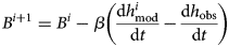
where B i is the bed elevation from the previous iteration and β is a scalar controlling the strength of bed updates applied in each iteration i. To obtain dh/dt mod, an ice flow model forced with a prescribed climatic mass balance $\dot {b}$ is run forward over a short time span dt (Frank and others, Reference Frank, van Pelt and Kohler2023). The rationale behind Eqn (1) is to find the bed which is consistent with the dynamic state of a given glacier as represented by its dh/dt obs field, implying that no steady-state assumption is made. Instead of applying Eqn (1) directly, however, one may also use available dh/dt observations and a climatic mass-balance product to compute the apparent mass balance $\tilde {b}$
 (Farinotti and others, Reference Farinotti, Huss, Bauder, Funk and Truffer2009), and feed that to the forward model instead of $\dot {b}$
 . $\tilde {b}$
 represents the climatic mass balance that would be needed for the glacier in its present shape to be in steady state. We do that here due to benefits in producing consistent input data (Section 4) which, considering that dh/dt obs is thus already incorporated into the mass balance that the forward model sees, requires us to set dh/dt obs = 0 in Eqn (1) when applying the bed updates.
To avoid introducing small-scale features in the bed solution not justified by the input data and to prevent fitting to errors regularization is needed (Habermann and others, Reference Habermann, Maxwell and Truffer2012). As detailed in Frank and others (Reference Frank, van Pelt and Kohler2023), this is done by adjusting the surface as a small fraction θ of the bed updates but in the opposite direction such that a new surface S i+1 is given by

The surface updates locally change the driving stress (e.g. where the bed becomes deeper, the surface height increases and thus the surface gradient and ice flow to surrounding gridcells is enhanced) resulting in a regular distribution of ice, while allowing the model to accommodate errors in the input data through small surface changes rather than large bed adjustments (Gudmundsson, Reference Gudmundsson2003). As shown in Frank and others (Reference Frank, van Pelt and Kohler2023), a larger value for θ leads to a smoother thickness field but it also increases the dependence on the initial bed because more of the dh/dt misfit is accommodated by surface updates rather than bed changes.
3.2 Ice flow model
The ice flow model used is the physics-informed deep learning-based IGM v2.0.4 ( Jouvet and Cordonnier, Reference Jouvet and Cordonnier2023) which builds on, yet significantly improves an earlier version (Jouvet and others, Reference Jouvet2022; Jouvet, Reference Jouvet2023). IGM represents a fusion between classical finite-element and deep learning methods in that the mass continuity equation
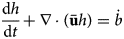
is solved where the ice flow velocities $\bar {{\bf u}}$ are obtained from a convolutional neural network (CNN). However, IGM not only relies on the CNN but also on a higher-order solver which is used to re-train the CNN in regular intervals during transient model runs.
Specifically, the ice viscosity-dependent higher-order ice flow approximation (Blatter, Reference Blatter1995; Pattyn, Reference Pattyn2003) including a Weertman-type sliding law (Weertman, Reference Weertman1957) is formulated as a minimization problem where a loss function seeks to find the ice velocity that minimizes the energy associated with the higher-order equations on a regular 2-D grid (eqn 18 in Jouvet and Cordonnier, Reference Jouvet and Cordonnier2023). While the solver finds the ice velocities by actually solving the minimization equation, the CNN seeks to obtain the same result, although through optimizing its weights. As such, the CNN learns the actual higher-order ice flow equation which as a result can be regarded as being encoded in the structure and weights of the CNN. This strategy is superior to the earlier versions of IGM that merely ‘copied’ the solutions obtained from a full-Stokes instructor model (Jouvet and others, Reference Jouvet2022) as it makes the CNN independent of an instructor model and the limited training data simulated with it. To ensure a close agreement between the emulator and solver solutions in transient simulations the CNN is retrained at a user-defined interval (here chosen to be every fifth model iteration). This means that at those instances, the solver is run to calculate the minimal energy associated with the current model state, followed by an update of the CNN weights such that the solution of the emulator is as close as possible to that of the solver. Due to the re-training strategy and the fact that the equation itself is learned, IGM can in principle be used with any spatial resolution and for any glacier type (as demonstrated by the application to an ice shelf in Jouvet and Cordonnier, Reference Jouvet and Cordonnier2023), in contrast to the previous IGM versions which were limited to a few possible resolutions and applications that were within the ‘hull’ defined by the training data (Jouvet, Reference Jouvet2023; Jouvet and others, Reference Jouvet2022). Thanks to the low computational cost of evaluating the CNN and because IGM is coded in a highly parallelized manner favourable for running on graphics processing units (GPU), IGM is efficient and allows us to use more advanced ice flow physics than previous studies on a regional scale.
3.3 Inversion workflow and parameter choices
To obtain an initial guess for ice thickness and bed topography, we use the perfect plasticity assumption (Nye, Reference Nye1952) given by

where h is the ice thickness, ρ = 910 kg m−3 is the ice density, α is the surface slope, g = 9.8 m s−2 is the gravitational acceleration and τ b is the basal shear stress. We estimate τ b based on Haeberli and Hoelzle (Reference Haeberli and Hoelzle1995) who established a parameterization relating glacier hypsometry to average basal shear stress along the central flowline of glaciers in the alps. Note that while this may be a crude approach, especially for ice caps, we do not see a significant impact of the initial ice thickness on the final result. Then, using the ice flow model IGM setup with observations of surface height, an apparent mass-balance field, a glacier mask, the initial guess of bed topography and a calibrated estimate on ice viscosity and sliding coefficient (Sections 3.4 and 4), we simulate 5000 model years in which we update bed and surface based on Eqns (1) and (2). The regularization parameter θ is 0.05 as in Frank and others (Reference Frank, van Pelt and Kohler2023).
To stabilize the inversion and aid convergence, we let β increase with each iteration i as in Frank and others (Reference Frank, van Pelt and Kohler2023) such that
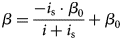
where β 0 is 1 and i s is 20.
This workflow, in general, allows to obtain a spatially distributed ice thickness map. However, due to imperfections in the representation of reality by the model and due to data errors, some ice may be leaving the glacier outlines laterally or at the front in each iteration, in which case other areas inside the domain remain ice-free. The magnitude of this ‘mass leakage rate’ can be calculated as the integrated climatic mass balance of the ice-free areas since that is the amount of mass missing to close the mass budget of a glacier inside its domain. To enable a closure of the mass budget, we add the total mass leakage rate divided by the glacier area to the specific apparent mass balance at each gridcell in the domain 2000 model years before the end of the simulation when the glacier already has reached a steady state. The ensuing advance of the glacier brings the mass budget closer to zero, although we note that in some cases, some of the added mass may be leaking out laterally or at the front too, meaning that areas within the glacier outline remain ice-free. While another round of mass-balance updates could resolve this, the fact that we do not know where exactly the leaking ice would have flown if the model and reality were perfectly aligned means that distributing the mass addition spatially uniformly carries the danger of much too-thick ice in some parts of the domain. Hence, we stick with one mass-balance update and instead fill holes in the ice thickness (i.e. where the ice thickness is smaller than 15 m; corresponding to on average ~8% of glacier area in this study) at the end of the inversion process through linear interpolation. In a final step, we apply a two-sigma Gaussian filter to the solution while taking into account local ice thickness and whether or not a given gridcell was interpolated. Specifically, we normalize the ice thickness field relative to a maximum value of 500 m. In the resulting norm raster (with values between 0 and 1), interpolated gridcells are also assigned 1, regardless of their thickness. The final ice thickness at each gridcell is then calculated as the sum of the smoothed ice thickness multiplied by the norm raster plus the non-smoothed thickness multiplied by 1 minus the norm raster. This approach allows to preserve small details in the bed shape where the ice is thin, while it removes such details where the ice is thick following the principle that there is an inverse relationship between the detail that can be possibly obtained through an inversion and ice thickness (Gudmundsson, Reference Gudmundsson2003; Raymond and Gudmundsson, Reference Raymond and Gudmundsson2005).
3.4 Calibration, validation and error estimation using thickness observations
3.4.1 Calibration
We calibrate our model results against all ice thickness observations (h obs) available for Scandinavia in the Glacier Thickness Database (GlaThiDa Consortium, 2020; Welty and others, Reference Welty2020) and a bed elevation model of Storglaciären (Björnsson, Reference Björnsson1981) ($n_{\text {obs\_total}} > 11\, 000$ ). This is done by tuning the region-wide rate factor A and the friction coefficient c of the Weertman sliding law (eqn 10 in Jouvet and Cordonnier, Reference Jouvet and Cordonnier2023). However, we exclude the observations of Jostedalsbreen from the region-wide calibration since we find that the errors in the modelled thicknesses are significantly larger than those at all other glaciers, indicating that Jostedalsbreen is not representative of the remaining glaciers (Section 5). Jostedalsbreen is calibrated separately based on its observations. The remaining observations cover ten glacier complexes (cf. Section 4) of different size, type and geographical distribution. Note that whether or not to correct the thickness observations for surface elevation changes that may have occurred since radar data acquisition has no appreciable effects on the results. This is in line with the general absence of trends in the mass balance of Scandinavian glaciers from the 1950s up until the 2000s (Holmlund and others, Reference Holmlund, Karlén and Grudd1996; Andreassen and others, Reference Andreassen, Elvehøy, Kjøllmoen and Belart2020). In this study, all mentions of thickness observations refer to the actual thickness values reported in the GlaThiDa. To allow constraining the two unknowns A and c against only one set of observations, we follow a similar approach as in Jouvet (Reference Jouvet2023) and assume that A cannot be larger than 78 MPa−3 a−1 (corresponding to the typical value used for temperate ice; Cuffey and Paterson, Reference Cuffey and Paterson2010) while sliding beyond a set minimum given by c = 100 km MPa−3 a−1 cannot occur for cold ice, i.e. when A < 78 MPa−3 a−1. Although this approach is a simplification that does not reflect the complex poly-thermal nature of glaciers in Scandinavia (Pettersson and others, Reference Pettersson, Jansson and Holmlund2003) as well as their possibly enhanced viscous deformation due to high liquid water content resulting from their maritime setting, it is chosen here since it allows to place A and c on one continuous scale with a unique solution for the combination of the two that minimizes the misfit to observations, and hence ensures an unbiased total ice volume estimate with respect to the observations.
To obtain the optimized A and c, we consider two different strategies: (1) minimizing the mean difference between modelled and observed thickness on a point-by-point basis for all observations pooled together. (2) For each glacier complex, determine the values for A and c which minimize the point-by-point bias for that glacier, and then select the A, c combination corresponding to the mean or median of the ranks of the sorted A, c combinations tested (note that for creating an evenly spaced A, c scale necessary for calculating means and medians of the A, c ranks, we find that setting a 5 MPa−3 a−1 change in A equal to a 500 km MPa−3 a−1 change in c is appropriate). While the former approach assigns equal weights to each thickness observation, the latter instead assigns equal weight to each glacier with observations. We find that following strategy 1 as well as taking the mean of the A, c ranks of strategy 2 yields the same optimal combination A = 70 MPa−3 a−1, c = 100 km MPa−3 a−1, whereas the median of strategy 2 gives A = 78 MPa−3 a−1, c = 100 km MPa−3 a−1. Given that two of the three indicators favour the former and since that A, c combination also yields overall better validation statistics, we settle for A = 70 MPa−3 a−1 and c = 100 km MPa−3 a−1. The obtained values are close to what one would expect for Scandinavian glaciers (A = 70 MPa−3 a−1 corresponds to an ice temperature of $\sim \!-0.6^\circ {\rm C}$ ) which are generally thought to be temperate but often feature cold surface layers (Pettersson and others, Reference Pettersson, Jansson and Holmlund2003; Andreassen and others, Reference Andreassen, Winsvold, Paul and Hausberg2012), suggesting that there are no major biases in our setup which need to be compensated by the calibration process. For Jostedalsbreen where we test a large parameter space of A and c to obtain the best validation statistics, we find an optimal combination A = 70 MPa−3 a−1, c = 1000 km MPa−3 a−1, i.e. elevated sliding is required to match the thickness observations best. Whether or not this represents a physical process is unclear given that the calibration of A and c against observations implies that all errors in the study setup (including those in the observations) are subsumed in these parameters.
3.4.2 Validation
The results are validated against the same set of thickness observations. Using the same set of observations for calibration and validation is not considered problematic here given that only Scandinavia-wide parameters are tuned against observations, while the validation is done on a point-by-point basis. We consider the RMSE and the mean absolute difference (MAD), both indicative of how far (in absolute terms) the modelled ice thickness is off from the observed one at any given point on a glacier; the mean difference/bias, showing whether the average ice thickness and thus total ice volume is over- or underestimated; and Pearson's correlation coefficient r between modelled and observed thicknesses which, too, indicates how well modelled and observed bed shapes agree. In addition, we calculate the slope of the linear regression between h mod and h obs to evaluate whether both high and low thicknesses are matched as well as the relative difference in variance $\Delta \sigma ^2 = ( \sigma ^2_{\text {mod}} - \sigma ^2_{\text {obs}}) / \sigma ^2_{\text {mod}}$ of ice thickness values at those locations where observations exist. The latter is a measure for how smooth the modelled bed shapes are in relation to the observations.
Furthermore, a direct volume validation is performed against five glacier complexes (Nordre Folgefonna, Søndre Folgefonna, Hardangerjøkulen, Blåmannsisen and Storglaciären) which have such dense radar coverage that their true volume can be assumed to be known (Björnsson, Reference Björnsson1981; Andreassen and others, Reference Andreassen, Huss, Melvold, Elvehøy and Winsvold2015; Ekblom Johansson and others, Reference Ekblom Johansson, Bakke, Støren, Gillespie and Laumann2022).
3.4.3 Error estimation
Since we calibrate the rate factor A and the sliding coefficient c, and through that the total ice volume, against observed thicknesses, an error estimation on the total ice volume can be made by varying A and c. If we had ice thickness observations that could be assumed entirely representative of the ‘true’ ice thickness distribution, tuning A and c so that the mean misfit with observations is zero would give an accurate Scandinavia-wide ice volume. However, since we do not know whether the thickness observations are representative, we ask the following question: If the sample of thickness observations was biased towards glaciers which are well-represented with high (low) values for A and c, what are plausible lowest (highest) values for the A, c combination? To resolve this question, we consider the results from strategy 2 above, and remove the highest and lowest A, c combination obtained for the ten glacier complexes. Based on that, we are left with a range (A, c) ∈ {(50, 100), (78, 1500)} which covers eight out of ten glacier complexes, and thus can be assumed plausible. With that, the results of the thickness inversion using A = 50 MPa−3 a−1 and c = 100 km MPa−3 a−1 form the high-end estimate for Scandinavian ice volume, while the values obtained using A = 78 MPa−3 a−1 and c = 1500 km MPa−3 a−1 mark the lower bound. To estimate the ice volume uncertainty of Jostedalsbreen, we assume the same range in A as for all other glaciers, but set c to 1000 and 2500 km MPa−3 a−1 in the upper and lower ice volume scenarios, respectively, following the results from the calibration where it was found that this glacier complex generally requires more sliding.
Further errors in the total ice volume could result from errors in the glacier outlines. Andreassen and others (Reference Andreassen, Nagy, Kjøllmoen and Leigh2022) suggest that an area uncertainty of up to 3% can be expected. If the outlines are too small, we do not know the ice thickness of the excluded areas. If the outlines are too big, it is likewise not possible to directly estimate how this would have affected the glacier thickness distribution inside these outlines, and thereby the ice volume overestimation of our result. Therefore, we simply assume that the volume uncertainty from glacier outlines is $\pm 3\%$ of the total ice volume.
Deriving a formal error estimate on local ice thickness for each gridpoint in the domain is difficult since the main error source likely are ice flow errors (i.e. when the model directs ice in a different direction than where it flows in reality) which are hard to quantify. However, thanks to the available thickness observations, the MAD between h mod and h obs can serve as an indicator for expected errors.
4. Input data
As input to the inversion, we require a DEM, spatially distributed climatic mass balance and dh/dt, as well as glacier outlines. Generally, we base our investigation on the RGI60 (RGI Consortium, 2017) and the glacier IDs therein which tie together the different input products. We, hence, do not use the updated outlines presented recently by Andreassen and others (Reference Andreassen, Nagy, Kjøllmoen and Leigh2022) for Norway for 2018–19 which have increased the number of glaciers by more than 2000 (covering an area of 48 km2) while the total glacierized area in the country reduced by 15% due to glacier retreat (Andreassen and others, Reference Andreassen, Nagy, Kjøllmoen and Leigh2022). This is because the climatic mass balance and dh/dt input datasets described below are not available for these new outlines. Since the glaciers added in the newer inventory are all small (the largest is 0.205 km2, and only 23 are larger than 0.1 km2; Andreassen and others, Reference Andreassen, Nagy, Kjøllmoen and Leigh2022), ignoring them here is not expected to have a significant impact on the modelled ice volume. The glacier outlines in the RGI60 for Scandinavia were acquired between 1999 and 2006 with a mean year of acquisition in 2003. However, a systematic misalignment with the topography is evident for the Swedish glacier outlines, possibly as a result of reprojection errors that occurred when the outlines were transferred from their original source to the RGI60 database. We correct these issues by re-aligning the outlines with the topography which yields a substantial improvement as confirmed visually. The new outlines are now included in the Global Land Ice Measurements from Space (GLIMS) database (Raup and others, Reference Raup2007; Paul and others, Reference Paul, Winsvold, Kääb, Nagler and Schwaizer2016) and in the newest release of the Randolph Glacier Inventory v7.0 which our results here hence are compatible with. Note that the original shape of each outline is unaltered (Fig. 2).
Input datasets used in this study alongside their date of acquisition. dh/dt from Hugonnet and others (Reference Hugonnet2021), climatic mass balance $\dot {b}$ from Rounce and others (Reference Rounce2023), DEMs from the Norwegian and Swedish mapping authorities, outlines from the RGI60 (RGI Consortium, 2017) corrected for an obvious misalignment with the topography in Sweden.

We use the national DEMs of Sweden and Norway in each country, respectively, with a 50 m resolution as provided by the national mapping authorities and stated elevation uncertainties of 5 m. The Norwegian DEM (Kartverket, 2013) is primarily from 2007, but has seen updates in different regions throughout the 2010s. The Swedish 50 m DEM (Lantmäteriet, 2022) is downsampled from the 1 m national DEM which was acquired between 2009 and 2019.
The dh/dt data are taken from Hugonnet and others (Reference Hugonnet2021) who compiled rates of surface elevation change for all glaciers on Earth. Following Huss (Reference Huss2013), these volume changes are converted to mass changes assuming a density of 850 kg m−3. The dh/dt data are available in 5 year bins from 2000 to 2019, but the signal in each bin alone may be contaminated considerably by noise. To avoid such issues we consider the entire 20 year period which yields the most stable signal.
The climatic mass balance $\dot {b}$ is taken from the global study by Rounce and others (Reference Rounce2023) who modelled $\dot {b}$
 in elevation bins for all glaciers on Earth for the 21st century. They performed an initial Bayesian calibration against the geodetic mass-balance estimates from Hugonnet and others (Reference Hugonnet2021) while validating against observations from the WGMS database (WGMS, 2022). For each glacier, we extract the years 2000–19 to match the dh/dt data temporally and create a distributed field of climatic mass balance by applying the elevation-dependent $\dot {b}$
 on the DEMs.
To close the mass budget of a glacier, it is necessary that:

where Ω is the glacier domain. Although Rounce and others (Reference Rounce2023) calibrated their modelled $\dot {b}$ against dh/dt from Hugonnet and others (Reference Hugonnet2021), the Bayesian approach does not guarantee that Eqn (6) is fulfilled. Further issues arise from the fact that there are spatial inconsistencies between dh/dt and $\dot {b}$
 in some places. For instance, dh/dt at the highest point in the accumulation area may be larger than $\dot {b}$
 , or comparably, dh/dt may be more negative than $\dot {b}$
 in some places in the ablation area. Given that a glacier cannot gain more in ice thickness than what it receives in accumulation where there is no influx from above, and that the glacier cannot thin more than what it loses from melt in the ablation area unless there are large changes in the ice dynamics which are not known to have occurred in Scandinavia, both cases most likely represent data errors. To mitigate such issues, we apply the following workflow (Fig. 3): first, we calculate the apparent mass balance (Farinotti and others, Reference Farinotti, Huss, Bauder, Funk and Truffer2009) as

Next, we bias correct $\tilde {b}$ such that $\int _{\Omega } \tilde {b} = 0$
 . Finally, we fit an elevation-dependent piece-wise linear function with two segments through $\tilde {b}$
 where we enforce the breakpoint at the apparent ELA. To ensure that $\tilde {b}$
 is monotonically increasing with elevation, we do not allow negative slopes in any of the two segments of the piece-wise fit, and replace the piece-wise fit with a linear fit if that should be the case. As a result of these steps, applied to each glacier individually based on the climatic mass balance and dh/dt inputs, we obtain a smooth $\tilde {b}$
 field that obeys Eqn (6) and is physically consistent.
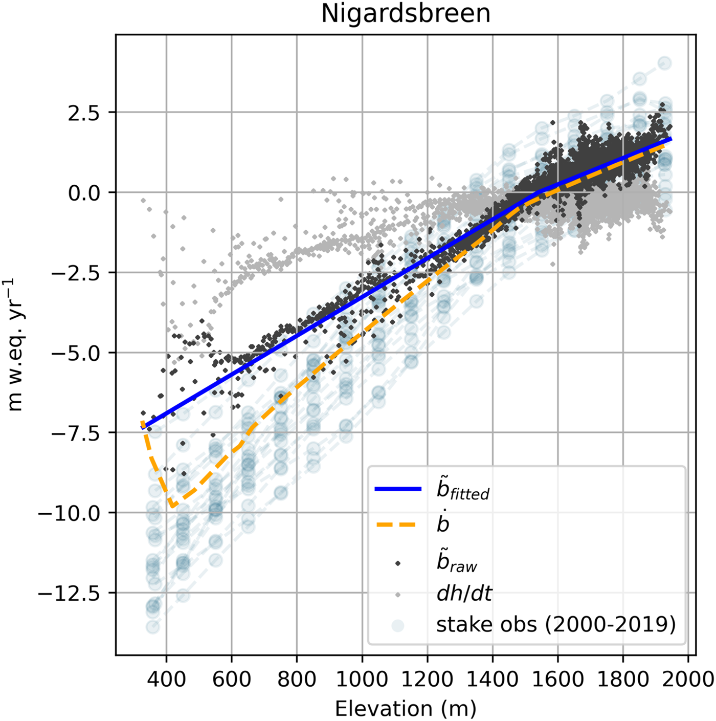
Methodology for computing the apparent mass balance $\tilde {b}$ using the example of Nigardsbreen. Based on the stake observations of mass balance for 2000–19 (where available) from WGMS (2022), Rounce and others (Reference Rounce2023) derived the elevation-dependent climatic mass balance $\dot {b}$
 . The difference between $\dot {b}$
 and the spatially distributed dh/dt (taken from Hugonnet and others, Reference Hugonnet2021) is the apparent mass balance $\tilde {b}_{\rm raw}$
 (Eqn (7)). $\tilde {b}_{\rm raw}$
 is then bias corrected to obey Eqn (6) (by 0.09 m w.e. for Nigardsbreen; not shown as it would not be visible) before a piece-wise linear function with the breakpoint at the apparent ELA is fitted through $\tilde {b}_{\rm raw}$
 to obtain the final apparent mass balance $\tilde {b}_{\rm fitted}$
 .
.
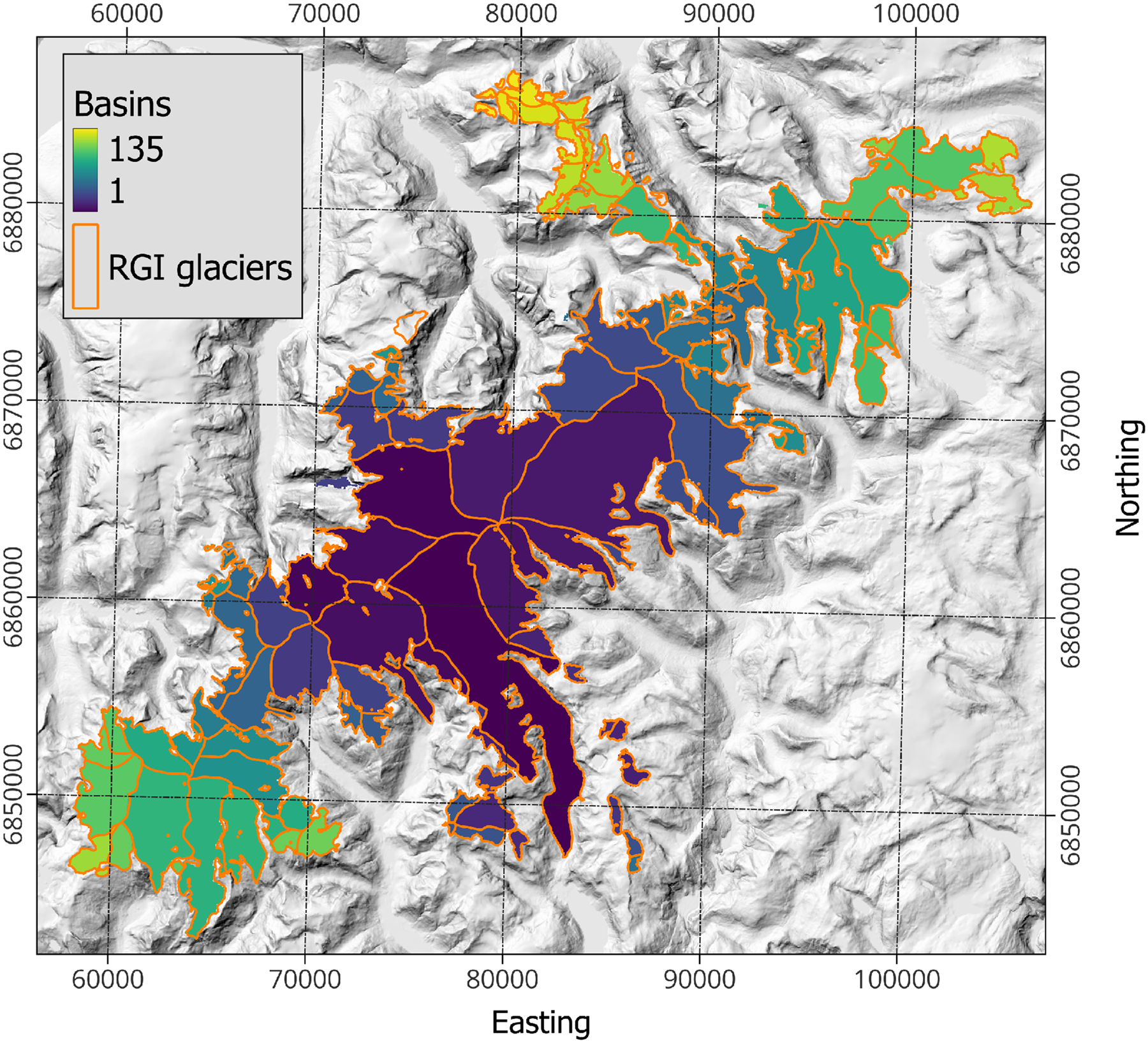
As a last step to input data preparation, we merge connected glaciers and all of their input fields together in one grid with 100 m resolution (Fig. 4). These glacier complexes are then modelled as one ice body which has the major advantage of preventing artificial boundaries and steps in modelled bed topography between connected glaciers. Particularly for ice caps where the RGI60 outlines may not always correctly delineate the actual flow units this is greatly advantageous as compared to modelling each RGI60 glacier individually.
Jostedalsbreen Ice Cap as an example of a glacier complex (coordinate system is UTM 33N). All 135 RGI60 glaciers are modelled simultaneously on the same grid to not introduce inconsistencies at the boundaries between flow units. Note that the glacier complex shown here includes some glaciers that are formally not seen as part of Jostedalsbreen (Andreassen, Reference Andreassen2022).
5. Results
5.1 Ice volume
We find an ice volume of 302.7 km3 for Norway and 18.4 km3 for Sweden, summing to a total of 321.1 km3 for all Scandinavian glaciers and ice caps. This corresponds to a sea-level equivalent of 0.81 mm (based on eqn 7 in Millan and others, Reference Millan, Mouginot, Rabatel and Morlighem2022). The mean glacier thickness is 113 m in Norway and 66 m in Sweden. The upper and lower bounds of ice volume estimated from varying A and c are 327.7/281.0 km3 for Norway, 20.6/16.9 km3 for Sweden and 348.3/297.9 km3 in total. By adding the uncertainty on glacier outlines, the ice volume for Norway is between 272.5 and 337.5 km3 ($h_{\text {mean\_NO}}$ in [102, 126] m), 16.4 and 21.2 km3 for Sweden ($h_{\text {mean\_SWE}}$
 in [59, 76] m) and 289.0 and 358.8 km3 for entire Scandinavia. This corresponds to a total uncertainty of ~±11%. The six large ice caps Hardangerjøkulen, Jostedalsbreen, Folgefonna, Svartisen-Vestisen, Svartisen-Østisen and Blåmannsisen, all located in Norway and covering 1238.2 km2 (42% of Scandinavian glacierized area), contain 61% of the total Scandinavian ice volume. In contrast, all Scandinavian glaciers with an area <0.5 km2 (n = 2420) together have an ice volume of 14.2 km3 (4% of total volume), while they cover 393.9 km2 (13% of total area). This small volume contained in the numerous little glaciers confirms that including the >2000 new very small glaciers (only 23 are larger than 0.1 km2) detected recently by Andreassen and others (Reference Andreassen, Nagy, Kjøllmoen and Leigh2022) would not have changed the overall Scandinavian ice volume appreciably. Indeed, to obtain a first-order estimate, we multiply the mean modelled thickness of all glaciers with an area smaller than 0.1 km2 by the total area covered by the new glaciers (48 km2) which yields an ice volume of 2.1 km3 which we are potentially missing. Considering individual RGI60 glaciers instead of the glacier complexes, the most voluminous glacier in Sweden is Salajekna with 3.2 km3, although it partially lies in Norway. The largest glacier by volume completely located in Sweden is the neighbouring Stuorrajekna with an ice volume of 1.8 km3. In Norway, the most voluminous glacier is Austerdalsisen (an outlet glacier of Svartisen-Østisen Ice Cap) with 13.6 km3. On that ice cap as well as on Jostedalsbreen we also find the largest ice thicknesses just above 600 m.
5.2 Bed shapes
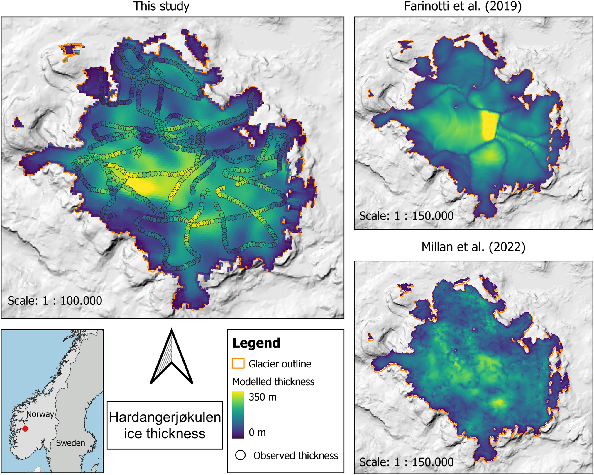
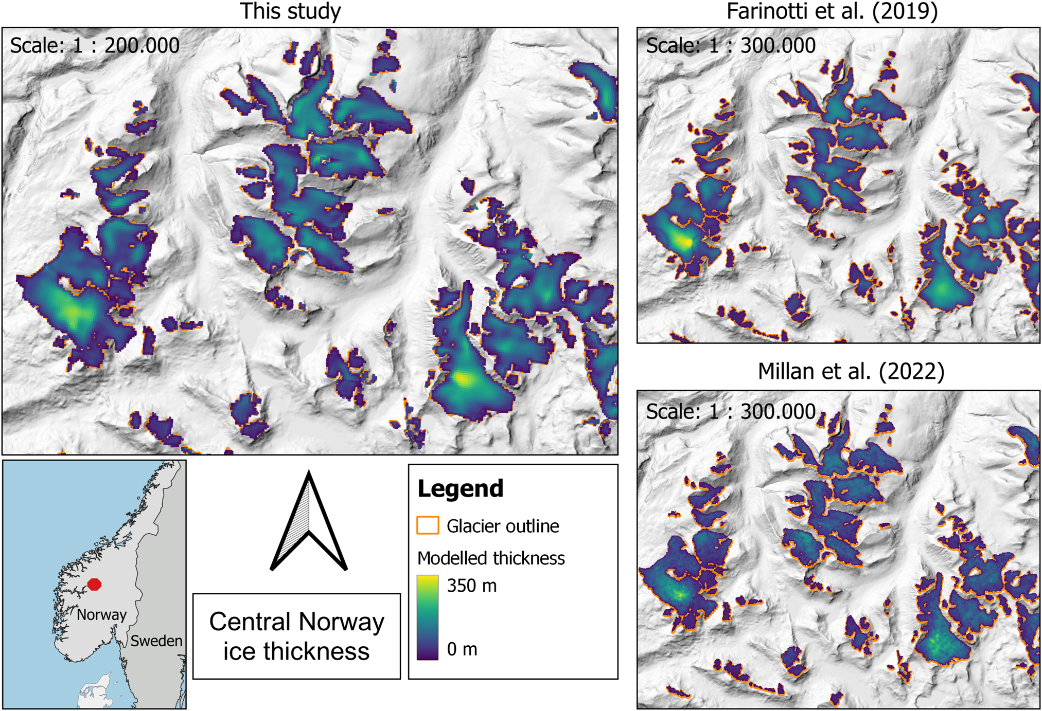
Besides ice volume, another main result of this study is a distributed map of bed topography and ice thickness for every glacier and ice cap in Scandinavia. While all results are available from https://zenodo.org/doi/10.5281/zenodo.10876057, we here show the example of an ice cap (Hardangerjøkulen) including observed thicknesses (Fig. 5) and of smaller mountain glaciers in central Norway (Fig. 6). We find that our modelled thickness field for Hardangerjøkulen is smooth but with clear variations in ice thickness, suggesting a variable subglacial topography. This agrees well with the observations, thus providing strong evidence that the obtained bed shape is realistic. Indeed, the general thickness pattern seems to be very well reproduced even where there are strong gradients in thickness, although the magnitude of certain subglacial features (e.g. the depth of a subglacial valley) may not always be matched exactly. Thanks to the approach of modelling the entire ice cap as one a bed topography free of artificial steps at the boundary of RGI60 flow units is obtained. For the central Norwegian mountain glaciers, our results likewise show an overall realistic pattern.
Modelled ice thickness for Hardangerjøkulen Ice Cap from this study as well as Farinotti and others (Reference Farinotti2019) and Millan and others (Reference Millan, Mouginot, Rabatel and Morlighem2022). Overlain on the results of this study are observations of ice thickness from the Glacier Thickness Database (GlaThiDa Consortium, 2020), originally collected by Sellevold and Kloster (Reference Sellevold and Kloster1964); Østen (Reference Østen1998) and Elvehøy and others (Reference Elvehøy2002).
Modelled ice thickness for mountain glaciers in central Norway from this study, from Farinotti and others (Reference Farinotti2019) and from Millan and others (Reference Millan, Mouginot, Rabatel and Morlighem2022).
5.3 Validation
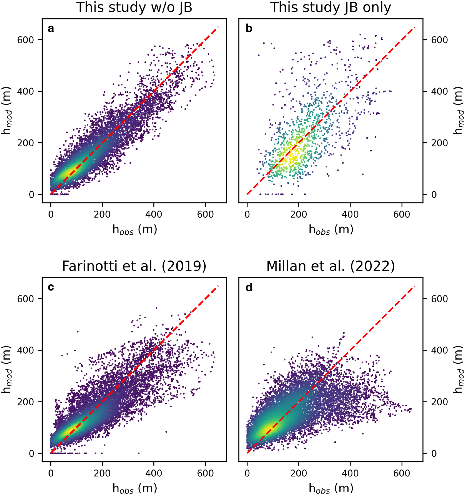
We find a good overall agreement between modelled and observed thicknesses with errors evenly spread around zero (Fig. 7a; Table 1). With the optimized values for A = 70 MPa−3 a−1 and c = 100 km MPa−3 a−1, the bias to all thickness observations pooled together is 0.8 m (for comparison, the bias obtained for the upper and lower ice volume estimates is −14.8 and 8.3 m, respectively). The MAD is 40 m, indicating that on average the modelled ice thickness at the observation locations is off by this value. Given a mean ice thickness of the observations of 165 m, this corresponds to an average thickness uncertainty of 24%. The correlation coefficient r is 0.87 demonstrating that the approach captures the Scandinavian ice thickness distribution very well, and it lends trust to the modelled bed shapes. We also compute the variance of ice thickness for all observations and the model output at those locations where there are observations; if the modelled variance is much smaller, the modelled bed is likely too smooth. For the same reason, we also consider the slope of the linear regression between h obs and h mod. A slope of one demonstrates that both low and high ice thicknesses are accurately captured. If the slope is significantly lower than one, as is often found for modelled ice thickness products, it usually implies that low thicknesses are over- and high ones underestimated, again due to too-smooth bed shapes. We obtain a variance that is 12% lower than the observations and a slope of 0.82 which is a good result compared to other studies (Section 6). This, too, indicates that not only the total ice volume but also the bed shape is well captured and realistic.
Correlation between modelled and observed ice thicknesses for this study for all glaciers except for Jostedalsbreen (a), for Jostedalsbreen alone (b), for Farinotti and others (Reference Farinotti2019) (c) and for Millan and others (Reference Millan, Mouginot, Rabatel and Morlighem2022) (d) with colours indicating point density and the red dashed line denoting the diagonal.
Descriptive statistics for thickness products from this study and previous work in relation to thickness observations

RMSE, mean absolute difference (MAD), mean difference/bias, slope of the linear regression between modelled and observed thicknesses, Pearson's correlation coefficient r and percentage difference in variance between h obs and h mod at those locations where thickness observations are available (Δσ 2).
We find the largest outliers in the thickness errors at Jostedalsbreen, even after calibrating it separately (Fig. 7b). Indeed, comparing modelled against observed thicknesses for all other glaciers together yields an MAD of only 35 m (corresponding to an average thickness uncertainty of 22%) and an RMSE of 46 m, indicating a close clustering of points around the diagonal (Fig. 7a). The 99th percentile of absolute errors is limited to 134 m for those glaciers meaning that there is virtually no point in space outside Jostedalsbreen where the true ice thickness should be off by more than this value. Meanwhile, the MAD for Jostedalsbreen alone is 82 m (35% of ice thickness).
For further validation, we consider glaciers that have such dense radar coverage that their ice volume can be established accurately through interpolation. We compare the observed ice volume as reported in the literature with the modelled values (Table 2) and find very good agreement. All modelled volumes are close to the observations and well within their uncertainty range, with no apparent bias.
Observed (V obs) and modelled (V mod) ice volumes for ice caps and glaciers in Scandinavia that have such dense radar coverage that their ice volume can be considered known
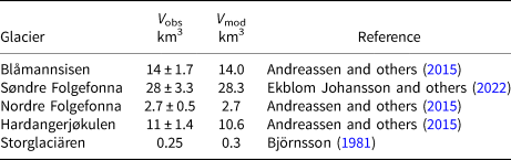
All values on V obs are directly from the literature except for Storglaciären where the ice volume was calculated by subtracting the bed topography by Björnsson (Reference Björnsson1981) (with no published error estimate) from a current DEM.
6. Discussion
6.1 Ice volume
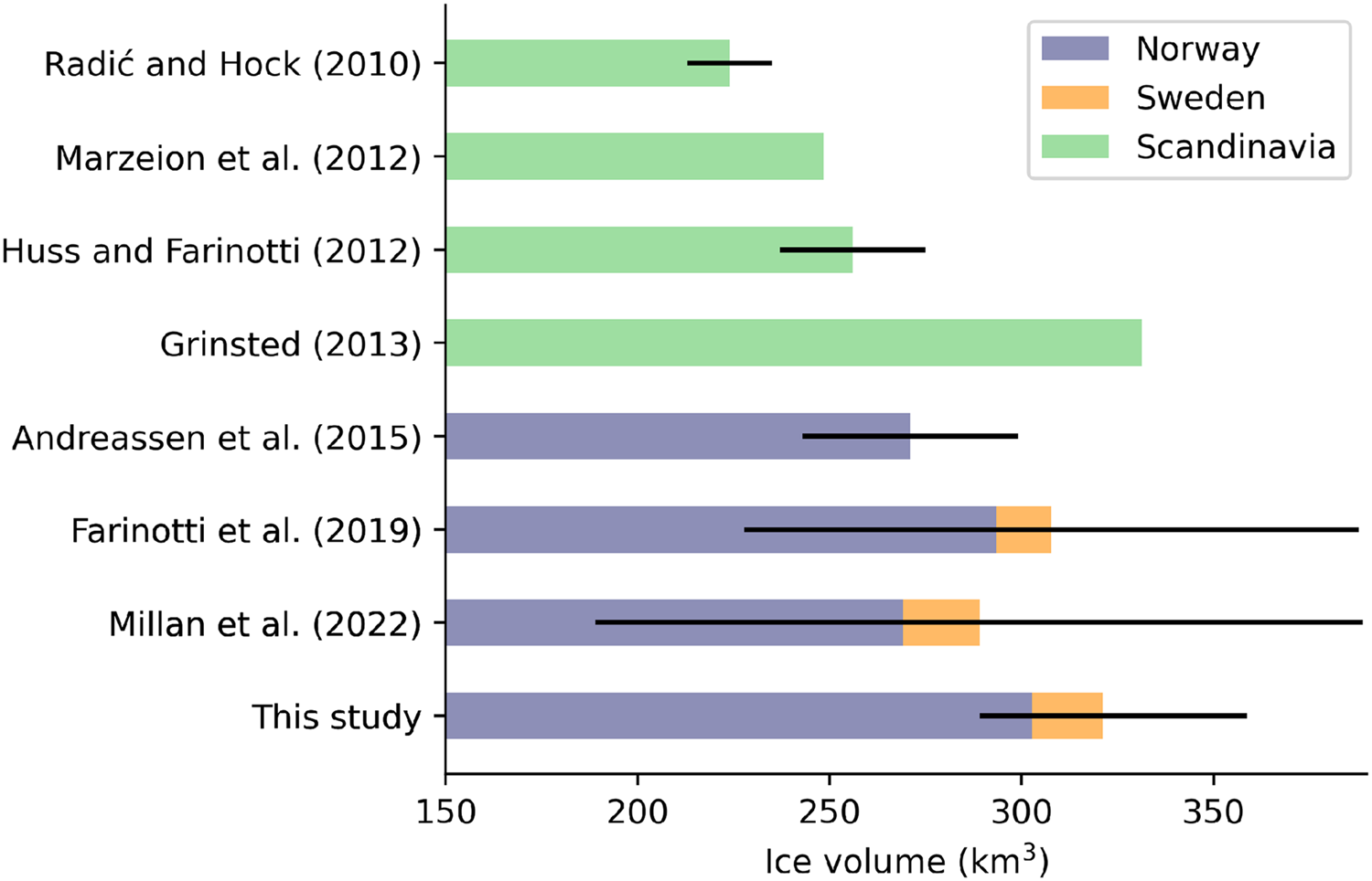
Our calibrated ice volume estimate of 321.1 km3 for Scandinavia with an estimated uncertainty range between 289.0 and 358.8 km3 is generally within the limits of previously published values (Fig. 8). However, it is significantly larger than the early works by Radić and Hock (Reference Radić and Hock2010); Marzeion and others (Reference Marzeion, Jarosch and Hofer2012) (which were based on volume–area scaling; Bahr and others, Reference Bahr, Meier and Peckham1997) and Huss and Farinotti (Reference Huss and Farinotti2012). It is also somewhat larger than what the more recent global studies by Farinotti and others (Reference Farinotti2019) and Millan and others (Reference Millan, Mouginot, Rabatel and Morlighem2022) calculated although the differences are small and well within the uncertainty bounds. The only previous study predicting a larger ice volume than this study is Grinsted (Reference Grinsted2013) with ~330 km3. Andreassen and others (Reference Andreassen, Huss, Melvold, Elvehøy and Winsvold2015) conducted a dedicated study on Norwegian ice volume combining different methods with observations and arrived at a ‘best guess’ of 271 ± 28 km3, although the total spread among methods was from 257 to 300 km3. This, too, tends to be less than what we obtain but again, the uncertainty ranges clearly overlap with ours (272.5–337.5 km3 for Norway).
Ice volume estimates from this study and previous work given either for Norway, Sweden or entire Scandinavia. Black lines indicate error estimates on the Scandinavian-wide ice volume (except for Andreassen and others, Reference Andreassen, Huss, Melvold, Elvehøy and Winsvold2015, where the error bar is on the Norwegian ice volume) as reported in the respective publications. Note the non-zero origin of the x-axis.
The only Scandinavian thickness products that are available as distributed grids and hence allow validation against observed ice thicknesses are the ones by Farinotti and others (Reference Farinotti2019) and Millan and others (Reference Millan, Mouginot, Rabatel and Morlighem2022). Both of them show a larger negative bias than our study (Table 1) indicative of an ice volume underestimation. Meanwhile, the close match that we obtain for the glaciers with known ice volume (Table 2) may suggest that our Scandinavia-wide uncertainties are rather conservative.
6.2 Bed shape
The early studies based on volume area scaling by Radić and Hock (Reference Radić and Hock2010); Marzeion and others (Reference Marzeion, Jarosch and Hofer2012) and Grinsted (Reference Grinsted2013) only yielded the mean ice thickness per glacier, no bed shape. The remaining works shown in Figure 8 produce distributed thickness fields although Huss and Farinotti (Reference Huss and Farinotti2012) and Farinotti and others (Reference Farinotti2019) completely or partially rely on flowline approaches at heart. As shown in Table 1, the product from Farinotti and others (Reference Farinotti2019) generally has larger errors than our results as indicated by the RMSE, MAD and r statistics. Also in terms of slope and Δσ 2, there are clear differences. The values obtained for our study (slope = 0.82, Δσ 2 = −12%) indicate that our modelled bed is smoother than reality, but given that there is a theoretical limit to how much detail in bed topography can be obtained through an ice thickness inversion (Gudmundsson, Reference Gudmundsson2003; Raymond and Gudmundsson, Reference Raymond and Gudmundsson2005), we find the results satisfactory. For Farinotti and others (Reference Farinotti2019) the slope and Δσ 2 are considerably lower (slope = 0.66, $\Delta \sigma ^2 = -37\%$ ) indicating that their computed bed is considerably too smooth. This is confirmed by Figure 7c where a clear tendency towards overestimating small thicknesses and underestimating large ones can be seen. A possible explanation for that is the ensemble approach underlying the methodology in Farinotti and others (Reference Farinotti2019) which naturally results in smoother results. The thickness product by Millan and others (Reference Millan, Mouginot, Rabatel and Morlighem2022) appears to align the least with the known ice thicknesses given the statistics in Table 1. As is also seen in Figure 7d, the modelled thicknesses are generally less precise than those of this study and Farinotti and others (Reference Farinotti2019), and there is a clear underestimation of large thicknesses. Given that Millan and others (Reference Millan, Mouginot, Rabatel and Morlighem2022) rely on remotely sensed velocity observations to compute ice thicknesses, the slow flow of most Scandinavian glaciers and consequently, the weak signal obtained is a likely cause for that. These difficulties in obtaining reliable ice flow velocities are also the reason why we did not use velocity observations to calibrate ice viscosity and sliding, as was suggested as a possible strategy for mountain glaciers in Frank and others (Reference Frank, van Pelt and Kohler2023). Experiments not shown here yielded consistently too-thin ice compared to observations.
Besides the statistical perspective, a visual inspection of the modelled thickness fields provides context on the quality of a thickness product. As concluded from Figures 5 and 6, our methodology produces realistic bed shapes both for ice caps and mountain glaciers. This is not necessarily the case for the products from Farinotti and others (Reference Farinotti2019) and Millan and others (Reference Millan, Mouginot, Rabatel and Morlighem2022) (Figs 5b, c). In the former, clear boundaries between RGI60 flow units as well as ‘stripes’ perpendicular to the flow direction can be seen for the ice cap Hardangerjøkulen. Both of these features are related to the underlying flowline approach which is generally known to perform poorly on ice caps (Huss and Farinotti, Reference Huss and Farinotti2012). For mountain glaciers, however, the results from Farinotti and others (Reference Farinotti2019) visually appear well confirming the strength of the methodology when applied to this glacier type. The results by Millan and others (Reference Millan, Mouginot, Rabatel and Morlighem2022) are somewhat noisy for both the ice cap and the mountain glaciers, again due to the methodological dependence on remotely sensed ice flow velocities. If taken at face value, these results would imply a highly unrealistic bed topography. Also the general thickness distribution of Hardangerjøkulen is not well captured as the observed thickness maxima of ~350 m are not reproduced.
The origin of the larger errors which we obtain at Jostedalsbreen (MAD = 35% of local ice thickness) compared to all other glaciers (MAD = 22%) is difficult to pinpoint. One possible explanation is that the thickness observations of Jostedalsbreen in the GlaThiDa date back to the 1980s (Kennet, Reference Kennet1989; GlaThiDa Consortium, 2020) with only limited documentation, making it difficult to assess data quality, potential biases or projection errors that could explain the large spread of the point cloud in Figure 7b. Indeed, there are some locations where all three thickness studies available (this study, Farinotti and others, Reference Farinotti2019, Millan and others, Reference Millan, Mouginot, Rabatel and Morlighem2022) unanimously indicate clearly larger values than the observations. Another reason could be that the low surface slopes of such a large ice cap are generally more inducive of large thickness errors in inversion products since bed undulations leave only small surface expressions (Gudmundsson, Reference Gudmundsson2003). Lastly, the topography surrounding Jostedalsbreen is generally very steep and spatially variable, suggesting that it could look similar under the ice which would naturally result in larger errors. We find that the error distribution for Jostedalsbreen is skewed with a median absolute error of 67 m (28% of local thickness), indicating that a few large outliers dominate the mean error. Therefore, if considering the median instead of the mean error, the value obtained is similar to the error that most thickness inversions yield which is typically at ~30% of the ice thickness (Farinotti and others, Reference Farinotti2017, Reference Farinotti2021).
6.3 Future perspectives
The methodology presented here is novel for Scandinavia in that it uses a full numerical ice dynamics model on a distributed grid to invert for ice thickness (Frank and others, Reference Frank, van Pelt and Kohler2023). Thanks to using dh/dt to infer subglacial topography, the bed shapes computed are in line with the dynamic state of the modelled glaciers, meaning that prognostic simulations of glacier evolution could be conducted without requiring any additional spin-up. Another benefit of the applied methodology is that it can readily profit from further improvements in input data quality which is not the case for approaches that are limited by the dependence on simplified ice physics. Indeed, all previous studies conducted in Scandinavia relied on volume–area scaling or simplified shallow ice physics, often applied along flowlines, in contrast to the higher-order physics in IGM. Experiments not shown here using a shallow ice approximation (SIA) model instead of IGM yielded unrealistic bed shapes which can be linked directly to the insufficiently complete ice flow physics with the SIA. Specifically, ice flow with the SIA is strictly downhill (Hutter, Reference Hutter1983), meaning that in an inversion context local topographic minima in the glacier surface accumulate ice and become very thick. Likewise, the convex across-flow profile of glaciers as seen in the DEMs directs ice flow with the SIA to the glacier margins. When doing an inversion this leads to larger ice thicknesses on the glacier margins than in the centre. While flowline approaches are not affected by these issues in the same way, these examples underscore the value of using sophisticated ice dynamics when modelling on a distributed grid.
Nevertheless, local errors in ice thickness remain which we attribute mostly to originate from errors in modelled flow directions as it has been shown that the methodology in general is not very sensitive to either initial conditions, parameter choices or climatic mass balance and dh/dt errors (Frank and others, Reference Frank, van Pelt and Kohler2023). While these erroneous flow directions may be the result of omitting terms in the higher-order model as compared to the full-Stokes equations (Blatter, Reference Blatter1995; Pattyn, Reference Pattyn2003), and hence of incomplete ice dynamics, they can also be caused by other factors related to input data or modelled processes. It has been shown that thickness inversions are highly sensitive to the input DEM as surface shape controls both flow directions and absolute thicknesses via the surface angle (Gudmundsson, Reference Gudmundsson2003; Chen and others, Reference Chen2022). Since we are using high-quality products from the national mapping authorities of Sweden and Norway we estimate errors associated with those to be overall small. However, even accurate DEMs do not immunize against certain topographic issues, for instance that in an inversion context, middle moraines protruding from the surrounding ice are interpreted as ice dynamical features formed by flow over a subglacial ridge, rather than as sediment lying on top of the glacier.
Further improvements in a future study could include the use of temporally more consistent input datasets which are currently not available. Due to the different time stamps of the inputs used here (Fig. 2) errors are likely introduced in the modelled thickness field, e.g. where parts of the DEM inside the RGI60 outlines show deglaciated terrain. Another difficulty arising from temporally inconsistent inputs is to establish what time our thickness product actually represents. Given that the mean year of the RGI60 outlines is 2003 (RGI Consortium, 2017), the mean of the climatic mass balance and dh/dt is 2010 (Hugonnet and others, Reference Hugonnet2021; Rounce and others, Reference Rounce2023) and an estimate for the mean for the DEMs is 2012, we suggest to refer to our results as representing the period 2003–12. Note, however, that assigning a time stamp to a product derived from temporally mismatched inputs is rather hypothetical, and so the given period is a mere estimate. If we accept that the computed ice thickness distribution corresponds to the abovementioned period, a first estimate on the Norwegian ice loss relative to 2018–19 when new glacier outlines are available for the country (Andreassen and others, Reference Andreassen, Nagy, Kjøllmoen and Leigh2022) can be made by considering the ice volume stored in those areas that have become ice-free over the time interval. We find that 18.5 km2 of ice are located outside the most recent glacier outlines, i.e. 6% of the Norwegian ice volume may have disappeared over an approximate time span of 6–16 years. Note that this is only a first estimate due to the difficulties of establishing a precise time stamp of our product as specified above, and because we do not take into account neither adjustments of ice dynamic processes nor thinning in those areas that have not become ice-free.
Lastly, more thickness observations would be of great help to improve future ice thickness inversions in Scandinavia. Currently, there is an over-representation of large ice caps among the ice bodies with observations (GlaThiDa Consortium, 2020). Since the ice caps are un-proportionally voluminous compared to the many smaller mountain glaciers (Section 5), this is not necessarily disadvantageous. However, more observations on smaller glaciers would allow for a better calibration there and could reduce the uncertainty on ice volume further. This is particularly true for Swedish glaciers where publicly available thickness observations are lacking almost entirely, meaning that the calibration for these glaciers is currently reliant on Norwegian observations obtained in a different climatic setting.
7. Conclusions
We here produced a new map of distributed bed topography and ice thickness alongside an updated ice volume estimate for each glacier and ice cap in Scandinavia. We anticipate that this product will be of benefit in a variety of applications, such as for water management in the context of hydropower production, for risk assessment of glacier lake outburst floods and landslides, for the planning of scientific projects, for the tourism industry and for future projections of glacier response to climate warming. The calibrated ice volume estimate for Scandinavia of 321.1 km3 with an uncertainty range of between 289.0 and 358.8 km3 is similar to, although slightly larger than, recent estimates proposed. Thanks to the novel methodology, this study is the first to provide realistic bed maps for all glaciers and ice caps in Scandinavia, outperforming previous studies (Farinotti and others, Reference Farinotti2019; Millan and others, Reference Millan, Mouginot, Rabatel and Morlighem2022) as shown by validation against thickness observations. Nevertheless, we find that the global perspective of the studies by Farinotti and others (Reference Farinotti2019) and Millan and others (Reference Millan, Mouginot, Rabatel and Morlighem2022) and their methodologically simpler approaches as compared to this study have not resulted in inaccurate ice volume estimates for Scandinavia. However, when it comes to the computed bed shapes the product by Farinotti and others (Reference Farinotti2019) suffers from clear issues on ice caps while the results by Millan and others (Reference Millan, Mouginot, Rabatel and Morlighem2022) are adversely affected by challenges in mapping the flow speeds of slow glaciers. We deem it likely that similar issues in these products are present in other regions on Earth, suggesting that future studies could seek to provide a further improved global ice thickness product.
Data
The distributed ice thickness and bed topography maps are available from https://zenodo.org/doi/10.5281/zenodo.10876057.
Acknowledgements
We thank David Rounce for kindly sharing climatic mass balance data with us. This research has been supported by Vetenskapsrådet (grant No. 2020-04319) and Rymdstyrelsen (189/18). The computations were enabled by resources provided by the National Academic Infrastructure for Supercomputing in Sweden (NAISS) at Chalmers partially funded by the Swedish Research Council through grant agreement No. 2022-06725.


 Open access