Introduction

Ice sheets respond dynamically to changes in boundary conditions, such as climate variations, basal thermal conditions, and isostatic adjustments of the underlying bedrock. The boundary conditions cause ice sheets to evolve towards a new equilibrium. The response is further influenced by feedback processes which may amplify or mitigate the ice sheet’s adjustment to the boundary conditions, or by internal dynamic-flow instabilities that may cause rapid changes in ice volume (Reference PatersonPaterson, 1994; Reference Rignot and KanagaratnamRignot and Kanagaratnam, 2006).

The near-surface air temperature is one of the boundary conditions and is considered to be a relatively straightforward meteorological variable to extrapolate or interpolate on climatic timescales. Temperature fields are, in general, continuous, and horizontal temperature gradients are typically low for long-term climatology, in which the effects of weather systems and fronts average out (Reference OhmuraOhmura, 1987; Reference GrotjahnGrotjahn, 1993). Vertical temperature gradients are much larger, and the common practice when extrapolating temperature fields to higher or lower elevations is to assume a constant atmospheric lapse rate (Reference OhmuraOhmura, 1987; Reference ReehReeh, 1991; Reference Ritz, Fabre and LetréguillyRitz and others, 1997). The choice is based on the average observed lapse rate in the free atmosphere and represents a typical moist adiabatic cooling rate. Despite their broad application, it is not clear that free-air lapse rates offer an appropriate estimate of slope lapse rates, which is the difference between near-surface air temperature at two locations divided by the difference in elevation (Reference Pepin and LoslebenPepin and Losleben, 2002; Reference Marshall, Sharp, Burgess and AnslowMarshall and others, 2007).

A measure of air temperature’s influence on annual ablation is the sum of positive degree-days (PDDs) (Reference OhmuraOhmura, 2001). The number of degree-days is defined as the total number of days when the temperature exceeds 0 ^° C in a year (Reference BraithwaiteBraithwaite, 1995). Many studies have used this type of model to calculate melt from mean monthly temperatures, which includes a magnitude for temperature fluctuations, σ _pdd, that can account for melt within a month with a negative mean temperature. This σ _pdd is the standard deviation of the near-surface air temperature and is mainly determined by the diurnal cycle and weather systems (Reference Lefebre, Gallée, van Ypersele and HuybrechtsLefebre and others, 2002). Values of σ _pdd in the literature range from 4.5 to 5.5 ^° C (Reference ReehReeh, 1991; Reference Ritz, Fabre and LetréguillyRitz and others, 1997; Reference Huybrechts and de WoldeHuybrechts and de Wolde, 1999; Reference Tarasov and PeltierTarasov and Peltier, 1999).

The primary motivation for developing a temperature parameterization is to use it with a PDD model to calculate spatial and temporal variability of the surface mass balance in numerical ice-sheet models without a full coupling between atmosphere and ice sheet, which takes a longer time to integrate numerically. Regional climate models would be more suitable to couple to an ice-sheet model in order to model the behaviour of the climate system on short timescales. Unfortunately, models of this type (Reference Box and CohenBox and others, 2006; Reference FettweisFettweis, 2007) cannot be applied in studies of the evolution of the Greenland ice sheet (GrIS) through ice ages with a sufficiently high spatial and temporal resolution, due to poorly constrained parameters, such as radiative fluxes and wind speed. This makes the combination of a temperature parameterization and a PDD model currently the best option for studies of the long-term evolution of ice sheets.

This study aims to improve the near-surface air-temperature parameterization for Greenland with the use of new observations from climate stations located on land, in the ablation zone and up to the dry snow in the accumulation zone on the ice sheet. The parameterization is tested by comparing melt-area observations from satellite algorithms with the calculated melt area from a PDD model. A comparison with a previous study by Reference Ritz, Fabre and LetréguillyRitz and others (1997) is also carried out, to test whether the new parameterization improves the calculated melt area extent.

Methods

Temperature parameterization

Observations from the Greenland Climate Network (GC-Net) (Reference Steffen, Box and AbdalatiSteffen and others, 1996; Reference Steffen and BoxSteffen and Box, 2001), the Geological Survey of Denmark and Greenland (GEUS) (Reference Ahlstrøm, Bennike and HigginsAhlstrøm and others, 2008) and the K-transect (Reference Van de Wal, Greuell, van den Broeke, Reijmer and OerlemansVan de Wal and others, 2005) (Table 1) and the automatic weather stations (AWS) of the Danish Meteorological Institute (DMI) (see www.dmi.dk for further information), are used to determine a new present-day near-surface air-temperature parameterization for the GrIS (Fig. 1). This study uses observations from locations on land, in the ablation zone and in the accumulation zone of the GrIS.

Fig. 1. The locations of the AWS on the ice sheet used in this study. Black lines indicate seven transects used for the slope lapse-rate

Table 1. Details of automatic weather stations (AWS) placed on the ice sheet

A mean monthly temperature is calculated from hourly observations each month in a given year for each station. Subsequently, the annual mean and the July mean temperatures are calculated for each station using all available mean values for the whole period (1996–2006; Table 2). The observations show that the slope lapse rate exhibits a strong seasonal variation, with a minimum in July. This variation needs to be taken into account in order to produce a realistic temperature field.

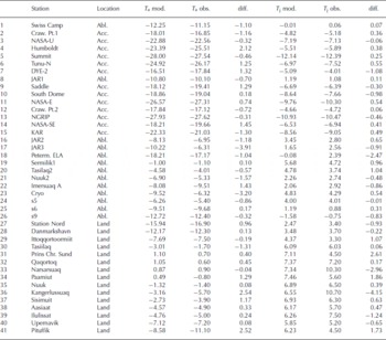
Table 2. A comparison between the modelled (mod.) temperature distribution and observed data (obs.) from the stations. T _a is the annual mean temperature and T _j is the mean July temperature. The difference (diff.) is calculated between the modelled and observed data. Acc., Abl. and Land denote stations located in the accumulation zone, in the ablation zone or on land, respectively

Following a study by Reference Ritz, Fabre and LetréguillyRitz and others (1997) the annual mean (T _ma) and July mean (T _mj) temperatures are parameterized as a function of altitude, z _s, latitude, φ, and longitude, λ:

((1))

((2))

where γ _ma is the annual mean slope lapse rate, γ _mj is the July mean slope lapse rate, c _ma and c _mj are coefficients determining the dependence on latitude, κ _ma and κ _mj determine the dependence on longitude, and d _ma and d _mj are constants. The values of the coefficients are given in Table 3. The coefficients were optimized by fitting the two parameterization functions to the observed mean temperature values (Table 2), using the least-squares method. The longitudinal dependence is new compared to the study of Reference Ritz, Fabre and LetréguillyRitz and others (1997) and is introduced in order to include the observation that temperatures are generally slightly colder in East Greenland than West Greenland for similar altitudes and latitudes. Mean monthly slope lapse rates (Table 4) are calculated between stations along seven different transects around Greenland in order to determine the variability of γ _ma and γ _mj used in the temperature parameterization. The transects are established between low-lying stations located in the ablation zone and stations in the accumulation zone on the GrIS (Fig. 1).

Table 3. Coefficients for Equations (1) and (2) and their root-mean-square difference (rmsd) in relation to the observed temperatures

Table 4. Mean monthly slope lapse rates and their standard deviation from seven transects (see Fig. 1)

Positive degree-days

The PDD method is based on the statistical relationship between positive air temperatures and the melting of snow or ice (Reference OhmuraOhmura, 2001). The percentage of days with melt, calculated on a monthly basis, is assumed to be equal to the probability that the near-surface air temperature exceeds 0 ^° C and the PDD factors relate the near-surface air temperature to melt of snow or ice (Reference BraithwaiteBraithwaite, 1995). Normally, large-scale melt models over Greenland calculate the number of PDDs by assuming an annual sinusoidal evolution of the air temperature (Reference GreveGreve, 2005).

The approach and the values of the degree-day factors are identical to those given by Reference GreveGreve (2005) and are briefly summarized here. The number of PDDs from the normal probability distribution around the monthly mean temperatures during the years is given as:

((3))

where t is the time, T air temperature and T _a ( ^° C) is the actual near-surface ( ^° C) is the annual near-surface melting temperature cycle. T _a is assumed to vary sinusoidally over time,

((4))

where A is taken to be 1 year.

Degree-day factors, β _ice, β _snow, are assumed to be different for ice and snow melt, and for warm and cold climate conditions. South of 72 ^° N the degree- day factors are assumed to be under warm conditions:

((5))

where and mm w.e.d^{− 1°} C^{− 1}. Cold conditions prevail north of 72 ^° N, and the mean July near-surface air temperature, T _mj, is used to calculate the degree-day factors:

((6))

((7))

where and mm w.e. d^{− 1°} C^{− 1}. The limiting temperature values, T _w = 10 ^° C and T _c = −1 ^° C, are used to calculate the limiting degree-day factors, which differentiate according to changes in T _mj.

The σ _pdd in the degree-day integral (Equation (3)) is different to that provided by Reference GreveGreve (2005). The value used here is smaller (σ _pdd = 2.53) than the value of 4.5 used by Reference GreveGreve (2005). The value of 2.53 is calculated from the mean value of the standard deviation of the mean monthly temperatures throughout the observation period (1996–2006).

The PDD model, combined with the new temperature parameterization, is used to model the current mean melt area extent of the GrIS. Results are tested against satellite-derived observations, that show the area of melt on the ice sheet (Reference Steffen, Nghiem, Huff and NeumannSteffen and others, 2004; Reference Fausto, Mayer and AhlstrømFausto and others, 2007; Reference FettweisFettweis and others, 2007; Reference Wang, Sharp, Rivard and SteffenWang and others, 2007). Three zones are defined: (1) the dry-snow zone where no occurs; (2) the melting-snow zone where melting occurs but all the meltwater is refrozen again as superimposed ice or internal accumulation; and (3) the runoff zone where meltwater is lost from the ice sheet. The melt area extent is then defined as the combined area of the runoff zone and the melting-snow zone. The definition corresponds well with the melt area extent categories of the satellite-derived observations because they use the reflected and emitted radiances to set up threshold values for no melting (dry-snow zone) and for melting of snow and ice (melting-snow zone and runoff zone).

Results

The inclusion of data from the GEUS stations provides a much clearer picture of the slope lapse rates (Table 4). The results from the transects show a great deal of variability, with a distinct seasonal cycle that has a double peak in winter. The largest slope lapse rates are seen in winter and the smallest in summer. The standard deviation of the slope lapse rate is also calculated, with the highest values in the winter and the smallest in the summer (Table 4). The maximum monthly slope lapse rate of −8.9 ^° Ckm^{− 1} occurred in February, and the minimum (−4.6 ^° C km^{− 1}) occurred in July. The relatively cold and variable winter temperatures in the interior of the GrIS results in steep slope lapse rates and high standard deviations in contrast to the summer (Table 4). In the summer, the near-surface air temperature can rise further in the interior than at the margin, since temperatures are low enough not to be limited by the ice surface reaching the melting point. The highest standard deviation values of the ablation season (3.0–6.0 ^° C) are found in May, June and September. The lowest values (<2.0 ^° C) occur in July and August.

The optimized values for γ _ma in Equations (1) and (2) (Table 3) are well within the standard deviation of the observed values. The discrepancy between γ _mj and the observations may be related to the fact that the observed slope lapse rates in Table 4 were calculated without using data from the land stations, while all the available data to determine the coefficients for Equations (1) and (2) were used.

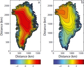
Figure 2 gives a visual presentation of the near-surface air-temperature fields computed from the new parameterization. It is clear that the altitudinal component dominates the temperature field. The figure shows that the effect of the latitudinal component changes with time of year due to the abundance of solar radiation in summer, or lack of it in winter. The effect of the longitudinal dependence can be examined by comparing the difference maps of Figure 3a and b (including longitudinal dependence) with those of Figure 4a and b (excluding longitudinal dependence). For example, the effect can be seen in the northwestern part of Greenland, where the temperatures in Figure 3a and b show higher positive differences than in Figure 4a and b. The new temperature parameterization, in general, also yields higher temperatures over the ice sheet for the annual case, whereas the July temperature only yields higher temperatures over the north and northwestern part of the ice sheet, due to a small latitudinal dependence combined with the longitudinal component. Similar higher temperatures also exist when not taking the longitudinal component into account, but with less difference in the northwestern part of Greenland. Figure 5a and b show the difference between the new temperature parameterization with and without data from the land stations. Without the land-station data the northeastern part of Greenland appears too cold compared with observations, due to a stronger longitudinal dependence, especially in the July temperature (Table 3). This is likely to be because of the sparse station data available in the north; land stations are therefore needed to predict the temperature more accurately.

Fig. 2. Parameterized (a) mean annual and (b) mean July temperatures. Dots show the locations of the AWS.

Fig. 3. The difference between the temperature parameterization for this study with a longitudinal dependence and that of Reference Ritz, Fabre and LetréguillyRitz and others (1997): (a) for the annual temperature and (b) for the July temperature.

Fig. 4. Same as Figure 3 but without a longitudinal dependence.

Fig. 5. The difference between the temperature parameterization for this study with and without land stations: (a) for the annual temperature and (b) for the July temperature.

Figure 6 shows the temperature difference between the observed values from the AWS and the temperature parameterizations of this study and those of Reference Ritz, Fabre and LetréguillyRitz and others (1997). The differences in temperature between the parameterization of this study and the observations are also given in Table 2. Comparing the new parameterization with Reference Ritz, Fabre and LetréguillyRitz and others (1997), both the annual and July temperature of the new parameterization show a better performance at 37 station sites out of 41, in relation to observations, corresponding to over 90%. The parameterizations by Reference Ritz, Fabre and LetréguillyRitz and others (1997) have a general overestimation at low elevations and a general underestimation at high elevations. The root-mean-square difference (rmsd) on the residuals from the temperature parameterization is given in Table 3. The values of the rmsd indicate a slight improvement when longitudinal dependence is included in the temperature parameterization.

Fig. 6. The temperature difference between the observed values from the AWS and the temperature parameterizations of this study and that of Reference Ritz, Fabre and LetréguillyRitz and others (1997). (a) The annual temperature and (b) the July temperature.

The annual melt extent was calculated with the PDD model using both the new parameterization and the temperature parameterization by Reference Ritz, Fabre and LetréguillyRitz and others (1997) for a spatial resolution of 10 km. The cut-off value for the Gaussian distribution in the degree-day integral (Equation (3)) is set to 1mm of melt, which implies that melt rates <1mma^{− 1} will be regarded as dry snow. The melt area extent for the parameterization by Reference Ritz, Fabre and LetréguillyRitz and others (1997) is 13.1 × 10⁵ km² (Fig. 7b). The melt area extent from the new parameterization is 6.6 × 10⁵ km² (Fig. 7a). The modelled melt area extent is then compared to a satellite-derived melt area extent. The satellite-derived melt area extent has a mean value of 4.6 × 10⁵ km² calculated over a 6 year period (2000–05) based on a moderate-resolution imaging spectroradiometer (MODIS) algorithm (Reference Fausto, Mayer and AhlstrømFausto and others, 2007). A mean value of ∼4.6 × 10⁵ km² for a period (1979–2002) of 24 years by Reference Steffen, Nghiem, Huff and NeumannSteffen and others (2004) and ∼5.2 × 10⁵ km² for a period (1979–2005) of 27 years by Reference FettweisFettweis and others (2007) is calculated using passive- and active-microwave data. Reference Wang, Sharp, Rivard and SteffenWang and others (2007) derive a melt area extent using the SeaWinds scatterometer on QuikSCAT, which is an active-microwave radar (Ku-band sensor). The QuikSCAT melt area extent has a mean value of 58% for the ice-sheet area of Greenland during the period 2000–04, corresponding roughly to a melt area extent of 7.1 × 10⁵ km². The largest difference in melt area extent between the modelled area and the satellite-derived area is ∼18% for Reference Fausto, Mayer and AhlstrømFausto and others (2007), and the smallest difference is 4% for Reference Wang, Sharp, Rivard and SteffenWang and others (2007). The four satellite-derived melt area extents agree reasonably well with the PDD model using the new parameterization, which gives confidence in its applicability.

Fig. 7. (a) The annual melt area extent for this study. (b) The annual melt area extent for Reference Ritz, Fabre and LetréguillyRitz and others (1997).

Discussion

Model parameterizations of this type have been applied often to the existing ice sheets of Greenland and Antarctica, and to those which covered the continents of the Northern Hemisphere during the Quaternary ice ages (Reference Huybrechts and de WoldeHuybrechts and de Wolde, 1999; Reference Tarasov and PeltierTarasov and Peltier, 1999; Reference GreveGreve, 2005). For example, Reference GreveGreve (2005) uses a glacial index, which is based on the results from ice-core data, to derive a time-dependent temperature forcing. A temperature distribution is then interpolated linearly between the present and the LastGlacial Maximum (LGM) values from a general circulation model. The glacial index scales the Greenland Icecore Project (GRIP) record to represent glacial and present conditions. The simulated anomaly from the glacial index is added to the near-surface air-temperature field over the whole region. The index is a useful tool, but it implies that the temperature distribution of Greenland can be interpolated between two climate extremes and that the climatic perturbation is the same for the whole ice sheet, which will not be the case. The parameterizations were primarily based on data from land climate stations and a few climate stations on the ice sheet. This may not give a clear picture of the evolution of the temperature field, due to different climatic and environmental conditions, and parameters that influence the temperature. However, the land-station data are needed to calculate the temperature parameterization, as without it the optimized coefficients would yield unrealistic temperatures, especially in the northeast.

The transition from land to ice further complicates the temperature distribution. Land and ice interact differently with the atmosphere. Over ice there is an ever-present shallow near-surface inversion layer, but land conditions will vary between convective and stable conditions (Reference GrotjahnGrotjahn, 1993). The observed slope lapse rate could be biased by frequent inversion layers that dominate the coastal climate under conditions of low clouds or sea fog coming from the ocean (∼400–500 m a.s.l.; Reference Box and CohenBox and Cohen, 2006). Reference ReehReeh (1991) includes a simple way to account for the coastal inversion layer in his parameterization to get a better fit to observations. It was necessary to include an inversion layer, because he used over 30 land stations and only 5 stations on the ice sheet, to parameterize his temperature field. The coastal inversion layer is not accounted for in this study because the majority of the stations used for the parameterization are located on the ice sheet. However, this could be a reason for the small discrepancy in the optimized coefficients in Equations (1) and (2) compared to the observations in Table 4.

The new temperature parameterization may not fully represent a climatological mean, as only limited data are available, obtained over different periods and sometimes for only a few months. This may therefore be responsible for a bias in the modelled temperature distribution. A proper validation of the parameterization is very difficult because all trustworthy observational data are used for optimizing the coefficients in Table 3. It could be argued that some of the station data should be used for validation. However, the scarcity of near-surface air-temperature observations and their uneven spatial and temporal distribution means that omitting any part of the dataset would cause a substantial change in the resulting optimized coefficients of Table 3.

To investigate interannual variability and the effect of varying spatial data coverage, the optimized coefficients in Equations (1) and (2) are calculated for each year in the data period (1996–2006; Table 5). The difference is quite high in some of the years when compared to the coefficients in Table 3, and the largest difference is seen in 1996 where the longitudinal dependence is negative, compared to the other years, for the July fit. However, all parameters obtained in this study (Table 3) fall within the standard deviations in Table 5. This gives us confidence that our parameters are representative of present-day conditions over the GrIS.

Table 5. Coefficients for Equations (1) and (2) and their rmsd in relation to the observed temperatures

The modelled melt area extent agrees reasonably well with the observed fit from satellite measurements (Reference Steffen, Nghiem, Huff and NeumannSteffen and others, 2004; Reference Fausto, Mayer and AhlstrømFausto and others, 2007; Reference Fettweis, van Ypersele, Gallée, Lefebre and LefebvreFettweis and others, 2007; Reference Wang, Sharp, Rivard and SteffenWang and others, 2007). The agreement depends primarily on the degree-day factors, σ _pdd and the cut-off value of the Gaussian distribution in the degree-day integral. In this study, the degree-day factors were not changed compared to the work of Reference GreveGreve (2005) (Equations (5) and (6)), which leaves σ _pdd and the cut-off value to account for the variation in melt area extent produced by the PDD model. The degree-day factors in the PDD model may show considerable spatial and temporal variability, as they incorporate all the energy-balance components into a single value for very different surface and climate conditions. It is therefore important to be aware of their limitations (Reference OhmuraOhmura, 2001; Reference HockHock, 2003).

The cut-off value of the Gaussian distribution was set to 1mm and it can be demonstrated that the sensitivity of the calculated melt area extent to this parameter is not very large. The cut-off value of 1 mm melt rate was chosen because it is assumed that a melt rate less than a snow grain size of ∼1 mm is not measurable (Bøggild Reference Bøggild, Reeh and Oerterand others, 1994).

It is commonly assumed that the values of σ _pdd span the interval 4.5–5.5 ^° C (Reference ReehReeh, 1991; Reference Ritz, Fabre and LetréguillyRitz and others, 1997; Reference Tarasov and PeltierTarasov and Peltier, 1999). In this study the value of σ _pdd = 2.53 ^° C was chosen, based on the mean value of the standard deviations of the mean monthly temperatures from each station located on the ice sheet. This is a direct reflection of the temperature variations observed at the climate stations on the ice sheet. Reference Lefebre, Gallée, van Ypersele and HuybrechtsLefebre and others (2002) reached a similar value for σ _pdd using a coupled atmosphere–ocean general circulation model for the southern part of Greenland. PDDs show a high sensitivity to changes in the value of σ _pdd, so it is important to constrain the value within observations. For example, it can be demonstrated that an increase of σ _pdd from 2.53 to 4.5 ^° C results in an increase of 33% in the melt area extent in the model (Fig. 7). This additional source of uncertainty is often not considered in other model studies, and their corresponding standard deviation is kept fixed or used as a tuning parameter in order to get a better fit to observations (Reference ReehReeh, 1991; Reference Ritz, Fabre and LetréguillyRitz and others, 1997; Reference Huybrechts and de WoldeHuybrechts and de Wolde, 1999).

Using the mean value of the standard deviations of mean monthly temperatures may not necessarily be the best choice for σ _pdd for modelling melt on short timescales. For example, using a value of σ _pdd determined for different sectors on the ice sheet may be a better choice. Such an approach would require more temperature observations from stations located on the ice sheet in order to improve the spatial coverage. An even larger problem occurs on long timescales, as we cannot know the standard deviation of the mean temperatures during the ice age. Therefore, we emphasize that the σ _pdd value is only valid for the present. A value of σ _pdd = 2.53 ^° C seems to be the best choice available for this study. The comparison between the modelled melt area extent and the satellite-derived measurements cannot qualify as a validation of the temperature parameterization because of the crude PDD method and poorly constrained degree-day factors, but the comparison tests the outcome so it can be used in large-scale ice-sheet models.

Reference Wang, Sharp, Rivard and SteffenWang and others (2007) find that the melt area extent, determined using their algorithm for enhanced-resolution QuikSCAT images, depends mostly on the variation in altitude, then on variation in latitude and least of all on the variation in longitude. This agrees with our findings. However, we have shown that longitude still plays a role in the temperature variation. The rmsd values indicate (see Results section and Table 3) that it contributes to a better agreement between model and observations. This gives an overall confidence in the inclusion of longitude in the temperature parameterization. Moreover, the spatial distribution of the AWS used in this study is, to the authors’ knowledge, the most comprehensive so far.

Calculating ablation using surface energy balance (Reference Van de WalVan de Wal, 1996; Reference Box and CohenBox and others, 2006) requires information about net radiation, wind speed, relative humidity and other poorly constrained variables that affect energy fluxes at the surface. Lacking input, there is no reason why energy-balance models should produce estimates of past or future ablation that are better than those based on the PDD model (Reference BougamontBougamont and others, 2007). To produce reliable scenarios for the GrIS, the ice-sheet models require temperature and precipitation data to reproduce the state of the ice sheet. The most reliable palaeoclimate proxies are air temperature and precipitation, which makes the PDD approach a powerful method for describing the surface mass balance in ice-sheet models.

Conclusion

A new temperature parameterization is used to estimate a melt area extent derived from a PDD approach. The temperature parameterization and the PDD model, which is based on physical and statistical considerations (Reference OhmuraOhmura, 2001), allow a fast integration speed in numerical schemes. The inclusion of new observational data and a longitudinal dependence in the temperature parameterization gives more accurate sensitivity values for elevation and latitude, and has produced a reliable near-surface air-temperature map. The standard deviation of the temperature observations, σ _pdd, is used as direct input for the PDD model. The value of σ _pdd = 2.53 ^° C is smaller than the generally used value of 4.5–5.5 ^° C. The strength of using the new σ _pdd is that it mimics the observed standard deviation of the temperature measurements from the climate stations more closely. A case study using the new temperature parameterization and σ _pdd = 2.53 ^° C showed that the PDD model provided a reasonable estimate for the mean melt area extent observed from satellites in Greenland. Acquisition of more temperature data and a longer time series is crucial to improve the temperature parameterization further; such an improvement closely follows the technical progress in such fields as ice-core drilling, remote sensing and the establishment of more AWS on the ice sheet. So far, the scarcity in the observational dataset precludes a proper validation of the temperature parameterization. More observational data will help improve this situation and are expected from the more than 30 AWS currently in operation on the GrIS.