1.1 Synoptic Paleoclimatology: A Bridge between Weather and Paleoclimate

Planetary or dynamic meteorology and climatology have been covered by several comprehensive textbooks, including Holton (Reference Holton1979), Peixoto and Oort (Reference Peixoto and Oort1992), Gill (Reference Gill1982), Barry and Carleton (Reference Barry and Carleton2001), Saltzman (Reference Saltzman2001), Vallis (Reference Vallis2017), Neelin (Reference Neelin2011) and Bigg (Reference Bigg2003). Similarly, the discipline of paleoclimatology has been comprehensively covered by several books, including Bradley (Reference Bradley1999), Cronin (Reference Cronin1999), Ruddiman (Reference Ruddiman2001), Bender (Reference Bender2013) and Ramstein et al. (Reference Ramstein2021). This book takes a different approach and focuses on applying the understanding of modern large-scale and synoptic climatology to the reconstruction of past climates, under the umbrella of ‘synoptic paleoclimatology’.

Synoptic paleoclimatology is an interdisciplinary approach that draws on atmospheric, oceanic and earth sciences to investigate and bridge the gap in the dynamics between paleoweather and paleoclimate. The traditional interpretation of the paleoclimate archive in terms of weather and climate has been based on a Lagrangian approach to understanding past air- or water-mass trajectories at a single site and their representation by parametric time series. Instead, examining the relationship of paleoclimate time series to the synoptic map through time allows an expanded view using a Eulerian approach akin to the climate field data generated by numerical modelling. The synoptic map has been the chief tool used to represent the array of modern weather-station data as a composite and is the most relevant tool for the representation of the array of paleoweather data. In the historical development of the synoptic map, orography was combined with the weather-station data array to identify the wind field as streamlines. While this is a Eulerian approach, the application of the synoptic map to paleoclimate investigations can also be a Lagrangian approach due to the lower temporal resolution (monthly and longer) of the paleoclimate signal being derived from ‘weather regime frequency’ and hence an approximation of air- or water-mass trajectories produced by an apparently quasi-stationary wind field. This concept is built upon the evolution of synoptic climatology (see Bergeron, Reference Bergeron1959) and applied to paleoclimatology. In a nutshell, the basis of this book is to view past climate change from the perspective of a deep understanding of circulation through the ‘weather map’ in much the same way as we would plan a modern-day sailing voyage route across the ocean (Figure 1.1).

Figure 1.1

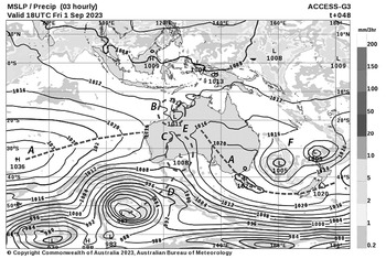
The weather map: the synoptic framework for viewing paleoclimatic change as responses to large-scale circulation modes, showing the forecast mean sea-level pressure (MSLP) and three-hourly precipitation for the Australasian and adjacent Indo-Pacific regions for 18 UTC, 1 September 2023 (accessed from www.bom.gov.au). The major surface-pressure features are shown: A – ridge and ridge axis; B – tropical low; C – secondary low; D – trough axis; E – col; F – subtropical low.

We use subjective and objective means to describe the ‘weather regime’ (WR) (described in Section 1.5) as a basis for the identification of large-scale flow patterns, their persistence or transience and associated weather characteristics. This is a spatial approach to paleoclimate and is complementary to the temporal approach characterised by time-series generation of paleoclimate attributes such as site, regional or global temperature, or precipitation. The synoptic paleoclimatology approach is based on the view that climate archives contain the ‘imprint’ of WRs on different scales, and time series of paleoweather and climate can be generated from an understanding of dynamical air- and water-mass transport paths and stochastic feedbacks.

Atmospheric variability is scaling and occurs on timescales from seconds to decades: for example (1) turbulence on seconds to minutes; (2) gravity waves on hours; (3) weather systems on days; (4) atmospheric blocking on weeks; (5) the Madden–Julian Oscillation on months; (6) the Quasi-Biennial Oscillation and the El Niño-Southern Oscillation (ENSO) on years; and (7) the North Atlantic, Arctic, Antarctic, Pacific Decadal and Atlantic Multidecadal Oscillations on decades (Williams et al., Reference Williams2017). The continuum between weather and climate is interrupted by a dynamic gap in the scales of processes and variability that extends from the limit of weather (7–10 days) through the subseasonal (10–60 days), to the multi-decadal (10–30 years), the centennial (100 years) and the millennial (1,000 years). The gap between weather and climate is dominated by low-frequency variability and has been termed ‘macroweather’ by Lovejoy and Schertzer (Reference Lovejoy and Schertzer2013). Macroweather is described in Section 1.5. This low-frequency variability displays weather-like spatial patterns of atmospheric pressure, winds, temperature and precipitation, and mesoscale sea-surface temperatures, currents and eddies.

The interpretation of the past century of instrumental weather observations is attached to the paradigm that 30-year periods define ‘climate’, yet this is an arbitrary period selected by the International Meteorological Organisation in the 1930s because there was high-quality data available for 1900 to 1930. We now know that the transition between weather and climate is much longer and that a 30-year period can correspond to one phase of quasi-macroweather oscillations such as the Pacific Decadal Oscillation (PDO, see Section 1.4). Therefore, we need to take a much longer view in paleoclimatology to define climate as an average of macroweather and for the duration of each stationary forcing period.

Modern climate analogues provide a basis for assessing the departure of past macroweather and climate from our own human experience. Hence, an understanding of the modern circulation at the global, large-scale (hemispheric) and synoptic (continental-ocean basin) levels is essential for a dynamic interpretation of past climate changes. A paleoclimate record includes up to three levels of information about the climate system. First-order information is recorded about the interaction of local-scale or microclimate processes with regional weather frequency defined by synoptic-scale patterns. Second-order information is recorded about the variability and persistence of large-scale climate modes in the atmosphere and ocean, such as storm tracks or ocean currents. The variability of large-scale climate modes ranges from seasons to centennial and is subject to internal system dynamics. Third-order information is recorded about changes in the mean state and seasonality of the climate system. These are externally forced changes or responses to planetary-scale feedbacks such as ice sheet growth and decay and land cover changes.

Often paleoclimate studies focus on interpreting the records as only changes in the mean circulation: for example, poleward–equatorward shifts in the westerlies, tradewinds or major convergence zones such as the Inter-Tropical Convergence Zone. To obtain a deeper understanding of paleoweather and paleoclimate dynamics, we need a sound knowledge of (1) global-scale seasonal patterns of pressure, wind field, air and sea-surface temperatures, precipitation, evaporation and sea-surface salinity; (2) atmospheric centres of action (quasi-stationary climatological anticyclones and cyclones and storm tracks) and associated wind-driven ocean currents; (3) timescales of variability and persistence; (4) atmospheric and ocean modes of inherent internal variability and their respective global teleconnection patterns; and (5) the past climatology of large-scale and synoptic-scale features including anticyclones, cyclones, storm tracks, planetary waves, air masses, clouds and convergence zones.

The driving force of the hierarchy of atmosphere–ocean circulation is the Earth’s energy balance and the resulting heat flux, temperature, precipitation, evaporation, salinity, cloud cover and sea-ice fields. The energy budget is highly variable across the latitudinal range since the Earth is an oblate spheroid and its spin axis is inclined (tilted) to the ecliptic plane around the Sun. The Earth’s axial tilt is at present 23.4° inclined to the plane. This means that at any given time latitudinal seasonal variations in radiation occur across Earth. Latitude and season determine the radiation balance at any point on Earth. The solar altitude determines the amount of radiation received. Over the tropics, where the Sun is close to the zenith angle, the mean annual absorption is ~50% of incoming solar radiation. In contrast, over the extratropics, this declines, reaching just ~20% at the poles due to low solar elevation and the high albedo of perennial snow and ice cover. The average energy flux for the combined atmosphere–earth surface system is positive between 40°N and 30°S and negative poleward of these latitudes. Hence, the heat flux, temperature, precipitation, evaporation, salinity, cloud cover and sea-ice fields are controlled by the seasonal latitudinal temperature gradients (LTG) and represent modern climate boundary conditions. These conditions, in turn, determine the general circulation and associated large-scale features and embedded weather or synoptic patterns.

From a paleo perspective, each component of the system needs to be resolved to understand climate evolution in response to changes in the Earth’s energy balance through time. A number of factors combine to drive paleoclimate change: external forces on the radiation budget produced by the astronomical progression in Earth–Sun orbital geometry, solar radiation output, changes in terrestrial forcing such as explosive volcanism, atmospheric gas composition, high-latitude ice sheet growth and decay and tropical ocean–atmosphere dynamics. The climate system is also forced internally by instabilities, interactions due to internal dynamics and feedbacks such as water-vapour temperature, snow and ice albedo, cloud and biosphere. Hence, synoptic paleoclimatology seeks to determine the shifts in regional atmosphere–ocean circulation and the associated synoptic features in relation to the time-varying LTG. (See Putnam, Reference Putnam2015, for a description of the glacial zephyr during the Last Glacial Maximum and Compagnucci, Reference Compagnucci2011, for the evolution of paleoclimate forcings and the atmospheric circulation for Patagonia and southern South America from the Jurassic to the present.)

Linking proxy weather and climate attributes to past atmosphere–ocean circulation patterns unlocks climate field analogues for evaluating forecast and hindcast model sensitivities to forcings, climate feedbacks, the physical robustness of modelled decadal- to millennial-scale variability, statistical artefacts in our understanding of climate mechanisms, and biases in the representation of the mean state of the troposphere or ocean. The end game for all paleoclimate studies is to be able to determine robust differences in the past climate and their physical causes, from those of the modern era and those in future climate projections.

1.2 Latitudinal Insolation, Temperature Gradients, and Paleoclimate Change

Essential for the study of paleoclimatology is the concept that the Earth’s energy balance has evolved through time, resulting in hot-house and ice-house climates. This evolution is due to changing atmospheric gas composition, plate tectonics and changing ocean circulation and solar irradiance receipts at the Earth’s atmosphere. The latter is a function of the orbital geometry of the elliptical Earth–Sun orbit. The respective periodicities for the orbital forcing of climate are 100 ka (eccentricity), 41 ka (obliquity) and 19/23 ka (precessional). Hemispheric impacts of eccentricity and precession are opposite and of obliquity are the same. This ‘orbital forcing’ is known as the ‘pacemaker’ of the climate system (Croll-Milankovich in Berger, Reference Berger1978; Imbrie and Imbrie, Reference Imbrie and Imbrie1979; Berger and Loutre, Reference Berger and Loutre1991), although the proxy record shows that scaling only roughly corresponds with the spectra associated with orbital forcing (Lovejoy, Reference Lovejoy2019).

Paleoclimate interpretations and modelling studies have shown that there is only a small variation in low-latitude temperatures, while there is a contrasting amplification in temperature change at high latitudes. This is recorded by the global ice volume fluctuations associated with the Quaternary ice ages, first at 41 ka and then at 100 ka cyclicity. Low-latitude climate varies through variations in eccentricity and precession of the equinoxes (monsoons and the ENSO phenomena). In contrast, high-latitude climate and the growth and decay of the ice sheets vary with the obliquity cycle, as do the temperature and salinity of the North Atlantic Ocean and the resulting Atlantic Meridional Overturning Circulation (AMOC). Consequently, paleoclimatological research has been somewhat polarised about the role of the tropics in climate change: for example, around the sensitivity of the Intertropical Convergence Zone (ITCZ) to small spatial gradients in sea surface temperature (SST), and the off-equatorial reach of changes in the ITCZ through the Hadley Circulation (Chiang, Reference Chiang2009), as opposed to the large temperature changes and ice sheet growth–decay cycles observed in the polar regions.

On paleoclimate timescales, varying latitudinal insolation gradients (LIGs) drive LTG, which in turn drive poleward–equatorward shifts in the key features of the general circulation such as the ITCZ, Hadley Cell, intensity and position of mid-latitude storms, subtropical anticyclone and extratropical low-pressure centres (Rind, Reference Rind1998; Jain et al., Reference Jain1999, cited in Davis and Brewer, Reference Davis and Brewer2009). Several researchers have focused on the orbital-forced and time-varying LIG between high and low latitudes to explain polar amplification and the ice-age cyclicity on Milankovitch timescales (Raymo and Nisancioglu, Reference Raymo and Nisancioglu2003; Davis and Brewer, Reference Davis and Brewer2009). The LIG is dominated by both obliquity (in summer) and precession (in winter). Obliquity controls the mean annual insolation, differential heating or LTG atmospheric meridional flux of heat, moisture, latent energy and ocean circulation. Accordingly, the LIG controls poleward energy fluxes, precipitation and ice volume at high latitudes. The LIG forcing of the LTG may cause the propagation of orbital signatures in the observed cyclicity of the ITCZ/monsoon, Arctic and Antarctic oscillations and ocean circulation in paleoclimate records (Davis and Brewer, Reference Davis and Brewer2009, figure 8) and on ENSO (Clement et al., Reference Clement1999). Obliquity-forced changes in the meridional temperature gradient have been shown to change the position and strength of the circumAntarctic westerly winds and the easterly flow of the Antarctic Circumpolar Current (ACC) and to influence the degree of ocean heat transport to the Antarctic ice sheet margin (Levy et al., Reference Levy2019, see figure 4 within).

Past climate changes are the product of orbitally forced shifts in the ‘latitudinal climatic zones, but more specifically the longitudinal variations caused by planetary and synoptic wave systems interacting with the earth’s surface’ (Barry and Carleton, Reference Barry and Carleton2001). The time-varying LTG is the baseline for understanding paleoclimate evolution and is responsible for determining the boundary conditions for the synoptic climatology through time that proxy climate variables record. The simplest way to think about the orbitally forced changes in the LTG and their impact on the synoptic climate is to deconvolve into periods of tropical expansion and contraction. Modelling studies indicate that an increased LTG is associated with an increase in global average surface winds, intensified subtropical jetstreams, a strengthened meridional Hadley circulation and drier subtropics (Rind, Reference Rind1998). This leads to an increased poleward moisture flux for ice sheet growth (Vimeux et al., Reference Vimeux1999). Another key finding from Rind (Reference Rind1998) was that increased poleward energy transport in the atmosphere is offset by reduced transport in the ocean.

The combination of orbital obliquity and precession controls the strength of seasonality in insolation, the equator–pole temperature gradient and the resultant tropical extent and strength of subtropical highs (Hays et al., Reference Hays1976; Davis and Brewer, Reference Davis and Brewer2009, figure 8; Mantsis et al., Reference Mantsis2013). A strong winter LTG produces changes in general circulation such as an equatorial shift in the subtropical ridge (STR) at 30°S; conversely, a poleward shift in the STR occurs during a weak winter LTG and a strengthened summer LTG. In general terms, a weak LTG is associated with reduced ice cover over Greenland, and the converse also holds (Davis and Brewer, Reference Davis and Brewer2009). A weakened summer LTG is associated with a poleward shift in the ITCZ, a strengthened summer monsoon, poleward subtropical anticyclones, warm subtropical gyre waters and reduced tradewind strength (Davis and Brewer, Reference Davis and Brewer2009). Modelling work by Clement et al. (Reference Clement1999), after Zebiak and Cane (Reference Zebiak and Cane1987) and Timmermann et al. (Reference Timmermann2007), illustrate the effect of the precessional cycle on the tropical mean climate, variability and the equatorial annual cycle, and the ENSO. The sensitivity of the tropics to orbital forcing and the non-linearity of ENSO’s response, together with its off-equatorial global teleconnections, highlight the role of the tropics in projecting climate changes across the globe (Chiang, Reference Chiang2009).

1.3 The Atmospheric Pressure Field and the Wind-Driven Ocean

This section is intended to be a brief introduction to the global atmospheric pressure field, its geographic centres of action (COA) and the role of wind and wind stress on global ocean circulation: particularly ocean gyres and major surface ocean currents, together with the surface ocean mixed layer. These topics are dealt with in detail in Chapters 2–4.

1.3.1 The Global Atmospheric Pressure Field

Knowledge of the general circulation of the atmosphere and ocean is the most fundamental platform for assessing future climate change or paleoclimate change. All changes in heat and water balance at a location on Earth are determined by the general circulation given energy-balance forcing. Gridded atmospheric pressure and wind-field data across the globe are essential to understanding both natural and anthropogenic-forced climate variability. The most detailed spatial array of atmospheric pressure and wind-field data spanning the troposphere and stratosphere is only available from 1979 with the advent of satellite meteorological observations. Prior to that, the number of observations (NOB) of station surface pressure and upper-air pressure decrease in time back to the earliest in 1775 CE. This causes a serious problem of spatial field heterogeneity through time.

During the past millennium, the expansion of Polynesian voyaging through the Pacific enabled the development of a cultural knowledge of the variable tradewind zones and westerly incursions into the subtropics. Later, European maritime circumnavigations including voyages to the Americas, Asia and throughout the Southern Hemisphere into the easterly tradewind zones and then into the westerly ‘anti-tradewind’ zones or ‘passage wind’ zones provided the earliest source of recorded and systematic, hemispheric-scale weather and climate observations. Captain Robert Fitzroy of the British Royal Navy set out the criteria for standardisation of marine weather observations (following on from Sir Francis Beaufort’s pioneering efforts with both a poetic and a numeric wind-strength scale) in 1863, following which the first regional and global maps of winds and currents were produced by Maury (1848–Reference Maury1860, also see Maury, Reference Levy1861) and Vladimir Köppen (1879) in sailing handbooks for each ocean basin (Deutsche Seewarte, 1885, 1892, 1897) (see the history of marine wind compilations in Lewis, Reference Lewis1996). The first global maps of atmospheric pressure and winds were published by Alexander Buchan (Reference Buchan1868, Reference Buchan1869) and later updated monthly and annual mean maps after the Challenger voyage (1873–1876) (Buchan, Reference Buchan1890). These global maps of winds, pressure, ocean currents and ice limits became standard products for ocean navigation and were published as Pilot Charts in the Admiralty Sailing Directions and in commercial volumes such as Findlay’s Sailing Directions for the regional oceans (e.g. the South Atlantic). The culmination of mapping the tradewind fields from shipping observations were the maps produced by Wyrtki and Meyers (Reference Wyrtki and Meyers1975a, Reference Wyrtki and Meyers1975b), prior to the expansion of instrumental ocean buoy coverage and later satellite altimeter-, radiometer- and scatterometer-derived global wind fields.

Prior to 1950, there is negligible pressure data for the Southern Hemisphere extratropics (see NOB figures at https://psl.noaa.gov/data/20CRv3_ISPD_obscounts/). Observational data over this region was significantly improved following the International Geophysical Year in 1957–1958. The lack of spatial homogeneity of atmospheric pressure data since the industrial revolution (~1850) to the satellite observation era (post 1979) means that it is difficult to accurately describe the pre-global-warming mean state of the atmosphere. The only complete spatial coverage is from 1979 onwards, and data from this period is contaminated by the additional anthropogenic forcing from industrial pollution: ozone, CO₂, other greenhouse gases and particulate aerosols. In addition, decadal-scale variability from internal climate dynamics means that choice of period for baseline climatology is biased towards the internal climate state. These shortcomings in the observational data and inherent biases need to be overcome by extending the spatial coverage of past meteorological variables, both instrumental and proxy sources.

Reanalysis of meteorological data using the assimilation of observations with climate modelling has attempted to hindcast gridded pressure and wind-field data across the globe. The most recent long-term reanalysis projects are the NCEP Twentieth Century V3 (1836–2015) and the ERA-40 and ERA5. These reanalysis projects are based upon the International Surface Pressure Databank (ISPD), which spans the period 1722–2015 (https://reanalyses.org/observations/international-surface-pressure-databank). The ISPD contains the established archives of meteorological variables together with recovered historical observations from the Atmospheric Reconstruction of Earth (ACRE) and Old Weather projects. Data over the oceans has been extracted to form the International Comprehensive Ocean–Atmosphere Data Set (ICOADS) and Simple Ocean Data Assimilation (SODA).

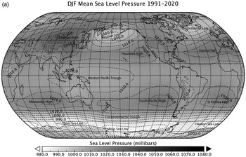
The highest-spatial-resolution representation of the modern mean atmospheric circulation is that produced from ground and satellite instrumental observations spanning the current climatological period 1991–2020. The surface pressure (sea-level pressure [SLP]) and wind fields are shown for the austral summer (December, January and February [DJF]) and austral winter (June, July and August [JJA]) in Figures 1.2 and 1.3, respectively.

Figure 1.2

Mean global MSLP climatology for the baseline period 1991–2020, (a) DJF and (b) JJA, showing the quasi-stationary centres of action (COA).

Figure 1.2a

Figure 1.2a Long description

Global map displaying mean sea level pressure for the period 1991-2020 during the DJF (December-January-February) season. Key pressure systems such as the Aleutian Low, Hawaiian High, and Western Pacific Trough are labeled. The map uses contour lines to indicate pressure levels in millibars, ranging from 980.0 to 1080.0 mb. Notable regions include the Circumpolar Trough, South Pacific High, and various sea level pressure lows and highs.

Figure 1.2b

Figure 1.2b Long description

Global map displaying mean sea level pressure for the period 1991–2020 during the JJA (June, July, August) season. Key pressure systems such as the Hawaiian High, Bermuda High, and others are labeled. The map uses contour lines to indicate varying pressure levels, with a scale ranging from 980.0 to 1080.0 millibars.

(NCEP2 reanalysis data obtained from https://psl.noaa.gov/data/reanalysis/reanalysis.shtml)

Figure 1.3

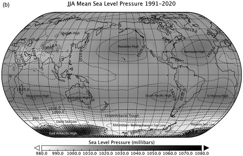
Mean global surface wind-field climatology for the baseline period 1991–2020, (a) DJF and (b) JJA, showing the wind direction (vector) and wind speed in graduated greyscale.

(NCEP2 reanalysis data obtained from https://psl.noaa.gov/data/reanalysis/reanalysis.shtml)

The most pervasive features in the global patterns of pressure and winds are the subtropical anticyclones and the zonal wind fields in the tropics (easterlies) and mid-latitude (westerlies) to subpolar (easterlies) regions. The pattern of surface winds is the expression of the meridional equator-to-pole cellular transfer of heat in the troposphere driven by the latitudinal insolation and temperature gradients. The global- to large-scale pressure patterns control the location and track of synoptic-scale disturbances such that there are preferred regions of cyclogenesis, storm tracks and eventual cyclolysis in both the tropics and the extratropics.

The global patterns of pressure can be subdivided into quasi-stationary centres of mean high pressure and mean low pressure, the COA. While the Buchan (1868–1888) pressure and wind maps first defined these semi-permanent features of the atmosphere, it was Teisserenc de Bort (Reference Teisserenc de Bort1883) who classified them as ‘centres of action’ and Hildebrandsson (Reference Hildebrandsson1897) who attempted to classify the climatology of each COA. The COA control mid-latitude weather and winds. The high-pressure COA are the quasi-stationary subtropical anticyclones primarily located over the regional ocean basins and are maintained by upper-level convergence and subsidence. The subtropical anticyclones generate high-pressure synoptic cells that travel eastwards and are intensified over continents. The COAs comprise the following and are shown in Figure 1.2:

• Northern Hemisphere: the North Atlantic High, 25–40°N, 20–45°W, with a clockwise seasonal displacement known as the Azores High in December and the Bermuda High in summer; the North Pacific High (Hawaiian High); the Greenland High; and the Siberian High (winter only), 45–50°N, 90–110°E.

• Southern Hemisphere: the South Atlantic High (St. Helena High); the South Indian High (Mascarene High); the Australian High; and the South Pacific High.

• Upper troposphere: the Bolivian High, 15–25°S, 60–70°W.

• Middle troposphere: the Botswana High, 15–25°S, 15–22°E; and the Bilybara High, 15–25°S, 115–125°E.

In addition, quasi-stationary subpolar anticyclones occur over the eastern Pacific in the Tierra del Fuego–Bellingshausen Sea region; and the western Pacific south of New Zealand. A quasi-stationary high-pressure COA known as the East Antarctic High occurs in the lower troposphere, above 850 hPa.

The low-pressure COA are depressions or troughs at locations where there is a high frequency of tracking mid-latitude cyclone centres, deepening of cyclones or centres of cyclogenesis and cyclolysis. These low-pressure COA represent the mean location of stationary disturbances of the zonal westerly flow and are maintained by upper-level divergence and uplift:

• Icelandic Low and Aleutian Low in the Northern Hemisphere;

• CircumAntarctic Trough (includes mid-latitude cyclone tracks and the Antarctic Coastal Lows, comprising the Davis Sea Low, Ross Sea Low, Amundsen-Bellingshausen Sea Low, Weddell Sea Low and Haakon Sea Low);

• West Antarctic Trough;

• Antarctic vortex, in the middle to upper troposphere.

The climatology of the oceanic and continental (Southern Hemisphere) COA are described in detail in Chapters 3 and 5 together with the associated weather regimes. This also includes the seasonal COA troughs located in the tropics that are produced by summer heating over the continents. This classification underpins synoptic typing in that COA represent the mean monthly to annual state of the regional climate and comprise an array of weather or synoptic types that occur on a daily frequency. In synoptic paleoclimatology, we aim to reconstruct the temporal evolution of the COA that is produced by the changing magnitude and frequency of weather regimes. In turn, the proxy record preserves the cumulative environmental impact of the magnitude and frequency of synoptic types.

1.3.2 The Wind-Driven Ocean

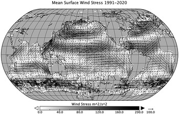
Surface ocean circulation is forced by the atmosphere (see overview in Talley et al., Reference Talley2011). The surface ocean is wind-driven since wind stress acts as a drag on the sea surface, setting in motion the ocean currents. The climatology of global surface ocean wind stress is shown in Figure 1.4. (Note that wind stress is a vector proportional in strength to the square of the wind speed, and its direction is in the direction of the wind.) The exchange of buoyancy fluxes of heat and freshwater between the atmosphere–ocean–atmosphere creates a contrast between lighter and denser water masses. This drives the subsurface thermohaline circulation. The ocean circulation is in geostrophic balance between the pressure gradient and Coriolis forces (Figure 1.5). Altogether, wind, heat and freshwater forcing drives meridional overturning circulation (MOC). Hence, large-scale and synoptic-scale weather, macroweather and climate all force mesoscale variability in ocean circulation.

Figure 1.4

Mean global ocean surface wind stress climatology for the baseline period 1991–2020, showing the wind stress direction (vector) and wind stress magnitude in graduated greyscale.

Figure 1.4 Long description

Global map displaying mean ocean surface wind stress from 1991 to 2020. The map features vectors indicating wind-stress direction and a greyscale gradient showing wind stress magnitude. Darker areas represent higher wind stress. Data sourced from ICOADS reanalysis.

(ICOADS reanalysis data obtained from https://psl.noaa.gov/data/gridded/data.coads.1deg.html)

Figure 1.5

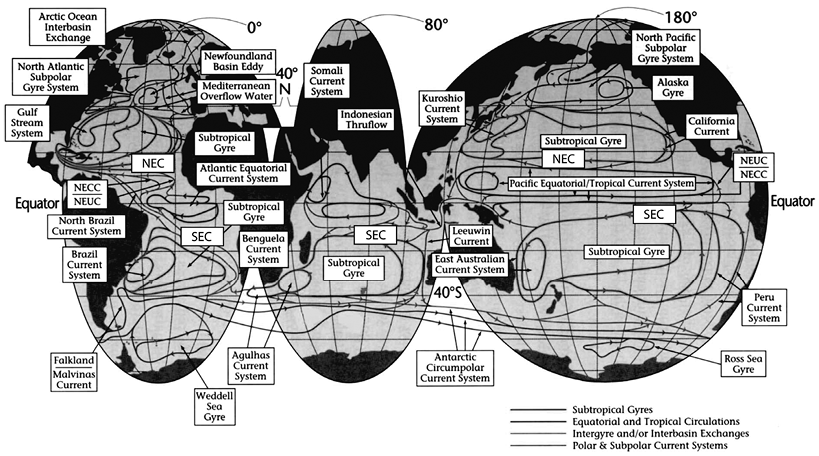
General surface ocean circulation including the major currents and gyres.

Figure 1.5 Long description

Global map illustrating major ocean currents and gyres. Key features include the Gulf Stream, Kuroshio Current, and Antarctic Circumpolar Current. Subtropical gyres are highlighted in the North and South Pacific, Atlantic, and Indian Oceans. The map also shows polar and subtropical current systems, equatorial and tropical circulations, and the Indonesian Throughflow.

(From Schmitz, 1996b.)

Opposing easterly tradewinds and mid-latitude westerlies drive ocean circulation as a system of rotating gyres (anticlockwise in the Southern Hemisphere and clockwise in the Northern Hemisphere). The subtropical gyres are centred on the subtropics and are connected by inter-ocean and interhemispheric currents, including the equatorial current system. The two major interhemispheric surface ocean transports occur in the Indonesian Throughflow from the North Pacific to the Indian Ocean and from the South Atlantic to the Gulf Stream. The gyres are asymmetric due to their rotation on a rotating Earth and the resulting Coriolis force (Stommel, Reference Stommel1948; Munk, Reference Munk1950), with the fastest flow along the poleward western sides of the gyres. The largest gyre is the circumpolar gyre driven by the ACC and connects the Southern Ocean to the Atlantic, Indian and Pacific Oceans via the Drake Passage.

While wind stress drives the ocean surface in motion, it is wind stress curl (vorticity) that drives the rotating gyres within the surface 1,000 m of the global oceans. The ocean gyres are located where the wind stress curl is zero. While the Coriolis force drives the surface current to the left of the wind direction in the Southern Hemisphere, and to the right of it in the Northern Hemisphere, friction and shear within the water column results in the Ekman Spiral, where the surface Ekman Layer transport is at 20–25° to the wind stress and where water at the base of the mixed layer is transported at 90° to the wind direction (after Ekman, Reference Ekman1905). Ekman transport controls the geography of upwelling and downwelling zones due to convergence and divergence of water masses (known as Ekman pumping). These convergence and divergence zones are discussed in Chapter 4 with respect to mesoscale ocean processes. The volume of water transported via Ekman pumping is known as Sverdrup Transport (Sverdrup, Reference Sverdrup1947). Positive wind stress curl causes downwelling and poleward Sverdrup transport (anticlockwise vorticity in the Southern Hemisphere). Negative wind stress curl causes upwelling and equatorward Sverdrup transport (clockwise vorticity in the Southern Hemisphere). Return flow via boundary currents is poleward in the subtropical gyres and equatorward in the subpolar gyres (see Chapter 4). A quote from Sverdrup (Reference Sverdrup1947, pages 325–326) highlights why the study of modern and paleo-wind fields in synoptic paleoclimatology are so important for understanding not only atmospheric variability but also ocean circulation: ‘the distribution of density and the mass transport by the accompanying currents … depend entirely upon the average stress exerted on the sea surface by the prevailing winds’, such that the meridional mass transport (Sverdrup transport) is proportional to the curl of the wind stress.

Global coverage of surface ocean currents, sea-surface temperature, sea-level atmospheric pressure (SLP), winds, salinity and waves has been derived from satellite tracked Lagrangian drifting buoys (see Global Drifter program www.gdp.uscd.edu, currently 1,300 drifting buoys in a 5 × 5 degree array, Risien and Chelton, Reference Risien and Chelton2008).

1.3.3 The Ocean Surface Mixed Layer

The ocean mixed layer extends for tens of metres of depth to at least 300 m down to the seasonal thermocline, where ocean temperatures are relatively constant and decrease with depth to the ocean bottom. The global ocean mixed layer depth climatology is shown in Figure 1.6 (see also Holte et al., Reference Holte2017). The temperature of the ocean mixed layer is largely controlled by solar radiation that penetrates a few tens of metres, together with vertical mixing with subsurface waters near the thermocline. The mixed layer loses heat to the atmosphere. Surface winds drive evaporation, and freshwater fluxes control surface ocean salinity. Overall, the ocean mixed layer is warm and has relatively low salinity, making it buoyant.

Figure 1.6

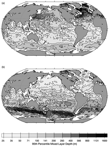
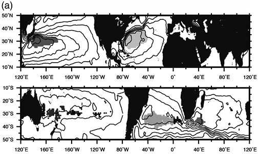
Maximum seasonal surface ocean mixed layer depth climatologies from the Global Ocean Surface Mixed Layer (GOSML) data compiled from ARGO float data for (a) mid-March and (b) mid-September: 95th percentile mixed layer depths contoured on a logarithmic scale (greyscale bar) from 25 to 1,600 m.

(From Johnson and Lyman, 2022, with permission from the American Geophysical Union.)

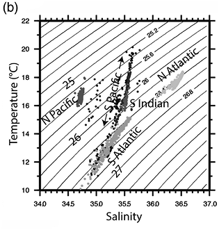
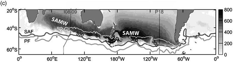
The highest wind speeds mix the surface ocean to the greatest depths, and hence mixing is greatest in the mid-latitudes during winter and in the North Atlantic Ocean, Northwest Pacific Ocean and Southern Ocean (to depths of between 400 and 800 m). These regions are where synoptic variability not only impacts the surface mixed layer and the gyre circulation but also modulates the surface water buoyancy and mixing that drives stratification and density-driven circulation at depth in the MOC. Strong wind mixing results in a constant turnover of surface water masses that drive the MOC together with tidal forcing. However, seasonal persistence creates ‘wind memory’ since seasonal water masses are advected both horizontally and vertically within the MOC, and hence, weather and macroweather anomalies are preserved and transported within the depth-integrated wind-driven ocean circulation. The regions where the synoptic forcing of the ocean is most pronounced are where the upper ocean mode waters form. Mode waters are geographically distinct water masses with vertically homogeneous temperature and salinity that form at the top of the permanent pycnocline (Hanawa and Talley, Reference Hanawa, Talley, Siedler and Church2001). The global ocean distribution of mode water masses is shown in Figure 1.7.

Figure 1.7

Mode water characteristics:

(a)

Distribution of the regional ocean basin subtropical mode water (STMW) mass areas.

(b)

Regional STMW masses mapped onto the temperature/salinity diagram together with the density surfaces.

(after Tsubouchi et al., 2016)

(c)

Location of subantarctic mode water mass formation north of the Subantarctic Front and the Antarctic Circumpolar Current, also showing the geographic distribution of the annual mean thickness (m) of SAMW together with the maximum mixed layer depth (MLD, m).

(From Li et al., 2021, with permission from the American Meteorological Society.)

The ocean responds to weather, macroweather and climate such that (1) ocean mixing in the surface layer by wind and buoyancy changes on hours to days; (2) the upper ocean responds to heating on months to years; (3) ocean eddy lifecycles on months; (4) ocean currents cross basins (1,000s of km) in decades; and (5) the MOC responds to atmospheric forcing on decades to millennia. In summary: the surface heat flux pattern is determined by wind-driven circulation; wind stress transport of heat fluxes by Ekman transport results in ocean heat gain from the atmosphere in divergence zones, and ocean heat loss to the atmosphere in convergence zones; and heat flux and ocean current changes are intensified in western boundary currents.

1.4 Climate Modes of Variability

1.4.1 Overview of Climate Modes

Climate modes of atmosphere–ocean variability have a sub-hemispheric to hemispheric spatial scale where quasi-periodic to periodic oscillations in regional atmospheric pressure are dynamically coupled to oscillations in air and sea-surface temperature, precipitation, wind, surface ocean currents, thermocline depth, and tropical and/or extratropical storm tracks (see Sun and Bryan, Reference Sun and Bryan2010). They modulate the strength, latitude and longitude of the COA. Hence, they are described as a teleconnection index between two or more COA that has an identified dynamical coupling. Beyond the primary COA, other correlated COA as defined by the projected spatial pattern are primarily associated with stochastic turbulence. Climate modes begin with multiscale convection organisation (such as tropical convective and mid-latitude baroclinic systems) and have an underlying physical mechanism that drives the inherent internal variability in the atmosphere and ocean, either by dynamics or by stochastic turbulence at both spatial and temporal scales.

Climate modes are typically a product of dynamics on short timescales from months to a year, and beyond that, they persist through stochastic scaling or long-term memory of the annual atmosphere and ocean weather (see Section 1.5 on the transition from weather to climate). The dynamical timescales are determined by the time for geostrophic restoring forces, such as Rossby waves and Kelvin waves to travel in the atmosphere and ocean; air–sea feedbacks on the temperature and wind fields; and transport within the ocean gyres and the MOC and stochastic turbulence forcing. The persistent climate modes consist mainly of scaling stochastic climate noise at interannual to decadal timescales, although some dynamical processes such as ocean convection persist at decadal scales in the extratropics (Franzke, Reference Franzke2009). Hence, paleoclimatolgists must consider that a proxy climate time series contains deterministic information mainly on shorter timescales and stochastic information on longer timescales. We will see that climate variability can be expressed in the form of WRs in Chapter 5. Climate modes of variability are described as the product of a spatial climate pattern and an associated climate index time series.

The connections between weather across the globe (teleconnections) and the availability of a decade of station pressure data in the late 1800s lead meteorologists to investigate statistical correlations and, subsequently, the discovery of weather oscillations, first in the atmosphere and then later as coupled atmosphere–ocean oscillations. The first discovery was the oscillation between pressure in the North Atlantic and Europe that gave rise to the identification of the North Atlantic Oscillation (NAO) between the Azores High and the Icelandic Low. Hildebrandsson (Reference Hildebrandsson1897) first published a global assessment with particular attention on oscillating pressure between Sydney, Australia, and Cordoba, Argentina (the precursor of the Southern Oscillation [SO]). These results were confirmed by Lockyer and Lockyer (Reference Lockyer and Lockyer1902, Reference Lockyer and Lockyer1904), who also constructed the first conceptual diagram of the Southern Hemisphere air circulation from a circumAntarctic view (Lockyer, Reference Lockyer1909, Reference Lockyer1910). Mossman (Reference Mossman1913) published the first compendium on Southern Hemisphere seasonal correlations of pressure, temperature and rainfall, and mapped the COA (Figure 1.8). Walker (Reference Walker1928) presented a global view and concluded that there were three major oscillations: (1) the North Atlantic Oscillation (NAO) between the Atlantic subtropics and the North Pole; (2) the North Pacific Oscillation (NPO) between the North Pacific High and the Aleutian Low, and its relation, the Pacific-North American Oscillation (PNA); and (3) the SO between the South Pacific and the land surrounding the Indian Ocean (Australia, India and Africa). Walker (Reference Walker1923, Reference Walker1928) based on the correlation between station pressure records (pressure COA), and the oscillating patterns in regional weather impacts (floods and droughts) described by rainfall COA, that appeared to oscillate on quasi interannual to biennial periodicity. Berlage (Reference Berlage1966) and Troup (Reference Troup1965) advanced the statistical robustness of the SO at seasonal fluctuations and further developed the Southern Oscillation Index (SOI), calculated as the difference in SLP between Tahiti and Darwin following more complicated multi-station indices. The Troup SOI that is used operationally in forecasting is defined in Eq. (1.1):

$\text{SOI}=10\frac{(P_{diff}-P_{diffav})}{\text{SD}(P_{diff})},$(1.1)

where P_diff = (average Tahiti MSLP for the month) − (average Darwin MSLP for the month), P_diffav = long-term average of P_diff for the month in question, and SD(P_diff) = long-term standard deviation of P_diff for the month in question, and the baseline period is 60 years (1933–1992) (Definition from www.bom.gov.au/climate/enso/soi/www.bom.gov.au/climate/enso/soi/.)

Figure 1.8

Early-twentieth-century atmospheric centres of action (COA) synthesis from the seasonal correlation of MSLP by Mossman.

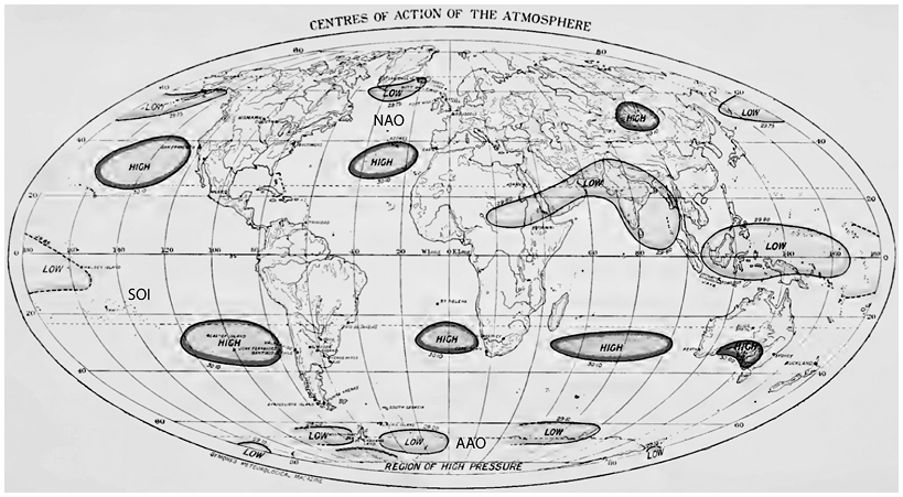
Figure 1.8 Long description

Global map illustrating early 20th-century atmospheric centres of action (COA) synthesis from seasonal correlation of mean sea level pressure (MSLP) by Mossman (1913). The map highlights regions of high and low atmospheric pressure, labelled with abbreviations such as NAO, SOI, and AAO, and shows pressure anomalies across various continents including North America, Europe, Africa, and Asia.

(1913)

The dynamics of the SO was first reported by Bjerknes (Reference Bjerknes1969) who proposed a coupled atmosphere–ocean interaction with dynamical feedbacks between the meridional Walker Circulation (the rising atmospheric motion and positive heat flux in the western tropics and the subsiding motion and negative heat flux in the eastern tropics, see Section 2.5) and the underlying ocean mixed layer and, hence, the identification of the El Niño-Southern Oscillation (ENSO) (see also Philander, Reference Philander1990; Allan et al., Reference Allan1996; Neelin et al., Reference Neelin1998). The dynamics of ENSO is described in Section 2.5.1.

Hence, the complex climate system can be broken down into the simplest configuration of understanding spatial and temporal variability in the three major ocean basins: the zonal east-west Indo-Pacific Ocean, the meridional north-south Atlantic Ocean and the zonal circumAntarctic Southern Ocean. The primary tropical ocean–atmosphere climate modes that describe seasonal to annual variability in ocean-basin SST are shown in Figure 1.9 and include The QBO and ENSO, the Indian Ocean Basin mode and the Indian Ocean Dipole (IOD) in the Indo-Pacific tropics (Saji et al., Reference Saji1999), the Atlantic Zonal Mode and the Atlantic Meridional Mode. The Pacific North American (PNA) and Pacific South American (PSA) modes that connect the tropics to the extratropics are discussed together with the dynamics of ENSO and the SAM in Section 2.5 (see Figure 2.17) and in relation to large-scale circulation and planetary wave modes in Chapter 3.

Figure 1.9

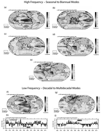
The major climate modes defined by global and basin-wide SST variability spanning: (a–e) high-frequency seasonal to biannual periods for 1958–2019 using ERSSTv5 data; (f–g) low-frequency decadal to multi-decadal periods for 1900–2014 after 10-year low-pass filtering using ERSSTv5 data. (a) DJF El Niño–Southern Oscillation (ENSO) mode with SST anomalies regressed onto the NINO3.4 time series. (b) March–April–May (MAM) Indian Ocean Basin (IOB) mode with SST anomalies regressed onto the IOB index time series. (c) September–October–November (SON) Indian Ocean Dipole (IOD) mode with SSR anomalies regressed onto the IOD index time series. (d) JJA Atlantic Zonal Mode (AZM) SST anomalies regressed onto the ATL3 time series. (e) JJA Atlantic Meridional Mode (AMM) SST anomalies regressed onto the AMM time series. (f) Pacific Decadal Variability (PDV) based on the tripole index (TPI) with SST anomalies regressed onto the TPI shown in (h). (g) Atlantic Multi-decadal Variability (AMV) based on the AMV index defined from Trenberth and Shea (Reference Trenberth and Shea2006) with SST anomalies regressed onto the AMV index shown in (i).

(From IPCC 2021, Appendix IV Modes of Variability, with permission from Cambridge University Press.)

The primary extratropical atmospheric modes of variability are the North Atlantic Oscillation (NAO) between the Atlantic subtropics and the North Pole; the Northern Annular Mode (NAM) or Arctic Oscillation (AO) and the Southern Annular Mode (SAM), also known as the Antarctic Oscillation (AAO); and the Arctic Oscillation (AO) and the North Pacific Oscillation (NPO). While, the AAO (SAM or High Latitude Mode) (Karoly, Reference Karoly1989, Reference Karoly1990; Gong and Wang, Reference Gong and Wang1999) was not statistically and dynamically revealed until post the 1970s, the precursor was observed by Mossman (Reference Mossman1913, Reference Mossman1916, Reference Mossman1918) in the South Atlantic Ocean region and seen as a southern counterpart of the NAO. Mossman observed a seasonal to interannual oscillation in pressure between Buenos Aires, Argentina and rainfall at Rosario, Brazil, with pressure at Orcadas, South Orkney Islands, and sea-ice concentration and extent in the Weddell Sea. He concluded that high seasonal (austral spring) rainfall in southern Brazil occurred during most northward sea-ice extent in the Weddell Sea when the South Atlantic storm tracks were deflected equatorward. He also identified relationships between pressure at St. Helena (South Atlantic High) and Punta Arenas (circumpolar trough). Therefore, Mossman’s observations were the first to describe the zonal oscillation in the COA and the mid-latitude storm tracks in the South Atlantic that we attribute to the SAM. Further, Gregory (Reference Gregory1904), Simpson (Reference Simpson1919a, Reference Simpson1919b), Griffith-Taylor (Reference Taylor and Joerg1928) and Kidson (Reference Kidson1928, Reference Kidson1946) produced the first spatial correlations between the mid-latitude Indo-Pacific and the Antarctica that demonstrated a zonal or annular pressure oscillation in the circumAntarctic. The SAM is now understood to be the internal atmospheric variability that is maintained by the eddy–mean interaction of the westerly flow (after Limpasuvan and Hartmann, Reference Limpasuvan and Hartmann1999, Reference Limpasuvan and Hartmann2000; Thompson and Wallace, Reference Thompson and Wallace2000; Thompson and Solomon, Reference Thompson and Solomon2002) with decadal ~20-year periodicity (Franzke, Reference Franzke2009) and hence is a primary mode in all paleoclimate timescales. The primary extratropical atmospheric modes of variability defined by the reanalysis data (NAO/NAM and the SAM) are shown in Figure 1.10.

Figure 1.10

The major extratropical atmospheric modes of variability defined in observations and reanalyses. (a) Boreal winter North Atlantic Oscillation (NAO) and Northern Annular Mode (NAM) extracted as the leading empirical orthogonal function (EOF) of DJF sea-level pressure (SLP) anomalies and regressed onto the leading principal component (PC) time series from 1959 to 2019. (b) The austral summer Southern Annular Mode (SAM) extracted as the leading empirical orthogonal function (EOF) of DJF sea-level pressure (SLP) anomalies and regressed onto the leading principal component (PC) time series from 1979 to 2019.

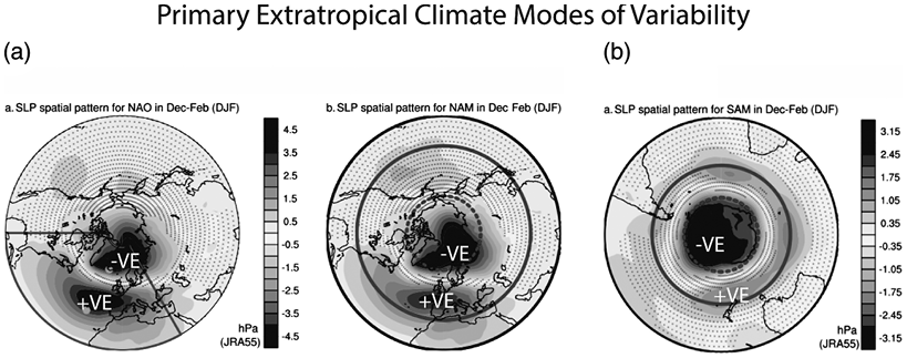
Figure 1.10 Long description

Graph showing primary extratropical climate modes of variability. Panel (a) displays the North Atlantic Oscillation (NAO) and Northern Annular Mode (NAM) patterns for boreal winter, indicated by sea-level pressure (SLP) anomalies from 1959 to 2019. Panel (b) illustrates the Southern Annular Mode (SAM) pattern for austral summer, indicated by SLP anomalies from 1979 to 2019. Each panel includes a polar map with pressure anomalies and key regions labelled.

(From IPCC 2021, Appendix IV Modes of Variability, with permission from Cambridge University Press.)

Subtropical modes of climate variability have been discovered in the South Indian Ocean (IOSD) (Behera and Yamagata, Reference Behera and Yamagata2001); South Pacific Ocean (SPSD) (Fauchereau et al., Reference Fauchereau2003); and South Atlantic Ocean (SASD) (Morioka et al., Reference Morioka2014) and summarised in Yamagata et al. (Reference Yamagata, Behera and Yamagata2016) and shown in Figure 1.11. These subtropical dipole modes all involve latitudinal shifts in the subtropical highs that are in response to both the ENSO-IOD and AAO phenomena. These modes can also be induced without tropical SST variability: The IOSD and SPSD are forced by the subtropical high response to AAO phases; the SASD is associated with a propagating Rossby wave generated by mid-latitude SLP anomalies in the western Pacific (Morioka et al., Reference Morioka2014). There is strong coherence between the IOSD and the SASD during the Austral summer (NDJF) (Fauchereau et al., Reference Fauchereau2003). Regional versions of these subtropical dipole modes occur over western Australia and the eastern Indian Ocean (the Ningaloo Niño: see Feng et al., Reference Feng2013; Kataoka et al., Reference Kataoka2014) and over south-west Africa and the south-east Atlantic Ocean (the Benguela Niño: see Shannon et al., Reference Shannon1986; Richter et al., Reference Richter2010).

Figure 1.11

Oceanic COA defined by sea surface temperature anomalies (SSTa) for the tropical and subtropical dipole modes.

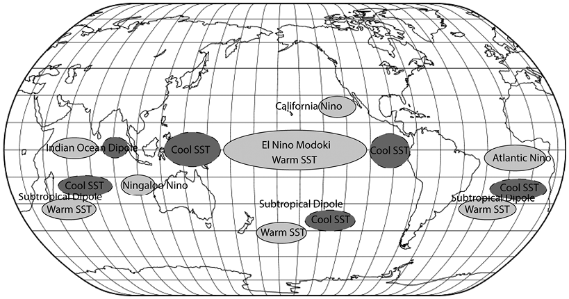
Figure 1.11 Long description

Global map illustrating oceanic climate anomalies (COA) defined by sea surface temperature anomalies (SSTa) for tropical and subtropical dipole modes. Key regions include the Indian Ocean Dipole, Ningaloo Niño, California Niño, El Niño Modoki, Atlantic Niño, and Subtropical Dipole, each marked with cool or warm SST areas.

(From Yamagata et al., 2016, with permission from World Scientific Publishing.)

I have included an account of this historical development of the understanding of climate modes of variability to show that these modes were initially defined with limited spatial and temporal instrumental data. Hence, they are robust features of the climate system and can be reconstructed with similar data limitations in paleoclimate as a measure of the mean state of the atmosphere–ocean system and its internal variability. While these climate modes are represented as independently and physically forced, they are components of the zonal and meridional atmosphere–ocean circulation, where climate signals are communicated via the large-scale atmospheric flow, ocean gyres and the MOC. The crucial element in any paleoclimate mode reconstruction is that the logic must be based on the behaviour of the primary COA as each mode projects onto distal regions via atmospheric and oceanic teleconnections that are mostly non-stationary through time and primarily a result of stochastic scaling (see Section 1.5.2).

The major climate modes have their own ‘flavours’ or varieties that are forced by regional wind anomalies. For example, ENSO can occur as an eastern Pacific (canonical) or central Pacific (Modoki) event with discrete pressure, wind, temperature, precipitation and salinity anomalies (Ashok et al., Reference Ashok2007; Ashok and Yamagata, Reference Ashok and Yamagata2009; Yeh et al., Reference Yeh2009). Cross-equatorial winds play an important role in driving the flavours of ENSO (Hu and Federov, Reference Hu and Federov2018), as do tropical Atlantic winds associated with the Atlantic Niño (Zebiak, Reference Zebiak1993), which can force a westward shift in the Walker circulation over the Indo-Pacific (McGregor et al., Reference McGregor2014; Li et al., Reference Li2015). Each of the Indo-Pacific and Atlantic tropical climate modes has a dynamically associated set of subtropical dipoles (Yamagata et al., Reference Yamagata, Behera and Yamagata2016). In addition, subseasonal to seasonal variability in tropical convection associated with the Walker Circulation and ENSO is described as the intra-seasonal Madden–Julian Oscillation (Madden and Julian, Reference Madden and Julian1994) and is associated with the Quasi-Biennial Oscillation between the troposphere and stratosphere (QBO) (Baldwin et al., Reference Baldwin2001). The atmospheric propagation of these Indo-Pacific tropical convective anomalies via Rossby Waves forces hemispheric scale variability in the extratropical Southern Hemisphere, known as the Pacific South American Modes (PSA1 and PSA2) (Mo and Higgins, Reference Mo and Higgins1998; Mo and Paegle, Reference Mo and Paegle2001) (see Figure 2.17).

Perhaps the most pertinent frequency of climate variability for synoptic paleoclimatology is low frequency due to the temporal resolution and smoothing of the paleoclimate archive. The two largest ocean basins, the Pacific and the Atlantic, exhibit low-frequency variability (decadal-multidecadal scale). These are known as the Pacific Decadal Variability (PDO, Mantua et al., Reference Mantua1997) and its SH variant the Interdecadal Pacific Oscillation (IPO, Folland et al., Reference Folland2002), and the Atlantic Multidecadal Variability (AMV, also known as the AMO) (Schlesinger, Reference Schlesinger1994; Mann et al., Reference Mann2014, Reference Mann2021). The PDV and AMV spatial patterns described by SST anomalies and their time series are shown in Figure 1.9. Decadal scale variability is inherent in the climate system and comprises the quasi-oscillatory slow-flow, physical behaviour, together with stochastic noise of the ocean system and long memory signal decay. The observed decadal-scale variability is a visible imprint of the scaling and long-range dependence combined with non-linear ocean–atmosphere interactions (Gil-Alana, Reference Gil-Alana2008; Graves et al., Reference Graves2015; Franzke et al., Reference Franzke2020).

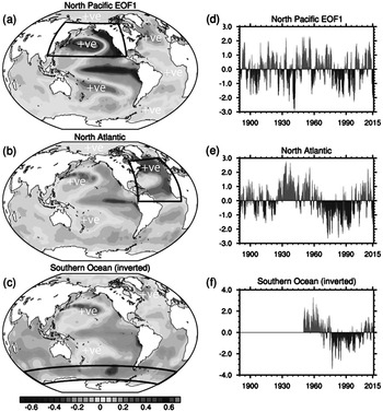
Wunsch (Reference Wunsch2003) showed that the quasi-periodic signals represent only a small fraction of the total climate variability. Most of the primary climate modes that represent EOF1 and 2 describe ~20–30% of the total climate variability variance. Many studies have focused on understanding these quasi-periodic signals, but the continuous variance spectrum is of equal significance (Franzke et al., Reference Franzke2020). Figure 1.12 shows the decadal climate variability for the North Pacific, North Atlantic and Southern Ocean basins by defining the leading EOF time series of monthly SSTa from ICOADS over the respective domains: North Pacific (20–70°N, 110°E–100°W, after Mantua et al., Reference Mantua1997); North Atlantic (0–60°N, 80–0°W, Trenberth and Shea, Reference Trenberth and Shea2006); and the Southern Ocean (50–70°S, 0°W–360°E, Fan et al., Reference Fan2014).

Figure 1.12

Multidecadal climate modes defined by the spatial and temporal characteristics of sea surface temperature anomaly (SSTa) variability in selected ocean basins. Left column: global SSTa* regression maps (degrees C) based on (a) the leading principal component of North Pacific SSTa,* (b) North Atlantic SSTa* and (c) inverted Southern Ocean SSTa. All indices were standardized prior to computing the regression maps. Index regions are outlined by black boxes. Right column: standardized 3-month running mean time series (1880–2015) of (d) the leading principal component of North Pacific SSTa,* (e) North Atlantic SSTa* and (f) inverted Southern Ocean SSTa. (From Deser and Phillips, Reference Deser and Phillips2017.)

* The global mean SSTa was removed prior to computing the time series and regression maps.

Pacific Decadal Variability (PDV) is a dominant mode and has attracted a large body of research to understand the drivers both in the instrumental and paleo records. PDV ranges from ~8 to 40 years for each La-Niña-like or El-Niño-like cancelling phase of low frequency variability. There are multiple drivers, and hence, it has underlying complex physical processes (that are poorly defined) and prevents deterministic approaches to forecast the interannual PDV variability and future phase or regime shifts. The PDV signal is the combination of macroweather turbulence and any forced component due to volcanism and/or solar irradiance variability (Earth’s mean temperature). Shorter decadal cycles with phases of 8–15 years are driven by the internal dynamics of the atmosphere and ocean system (scaling turbulence from eddies, horizontal and vertical currents and gyres). The simplest explanation is that these short PDV cycles develop as a cumulative residual of largely independent ENSO events (1–2 years) in the tropical to subtropical ocean. This is manifest in the form of a build-up or release of upper ocean heat content between 5° and 30° latitude in the south-west and north-west Pacific Oceans (Power et al., Reference Power2021). In the Australian region, a long-term build-up of subtropical ocean heat content in the Tasman Sea and out to the Cook Islands in the south-west Pacific drives a La-Niña-like climate (Meehl et al., Reference Meehl2016).

Since individual La Niña events tend to last longer than El Niño events (ENSO magnitude-frequency asymmetry, Power et al., Reference Power2021), it is consistent that La-Niña-like PDV events persist for longer than stronger El-Niño-like PDV events. These shorter internal cycles in the climate system impact both the western and eastern tropical Pacific with teleconnected impacts on the mid-high latitude wind fields and storm track in both hemispheres. To complicate matters, emerging observations and model output indicate that mean-state changes in the tropical Pacific Ocean may be remotely forced by the SST pattern and associated tradewind fields in the tropical Atlantic.

Longer multi-decadal cycles with phases of 15–40 years are driven by external forcing such as intermittent volcanic eruptions with residual cooling of the sub-surface ocean, slowly increasing greenhouse gases and varying anthropogenic aerosols emission. These influence cloud cover and the solar radiation budget in the atmosphere. The slower dynamics involves the slow adjustment timescale of the wind-driven ocean, particularly the circulation connecting the subtropical and equatorial regions. The possible dynamical mechanisms for the low frequency variability involve the slow propagation of water mass anomalies around the ocean gyres and the MOC, together with complex air–sea interactions (see Newman et al., Reference Newman2016 for the PDO, and O’Reilly et al., Reference O’Reilly2016 for the AMV). Simplistically, the decadal scale variability is produced by ocean circulation feedback from the subtropics, and the longer multi-decadal variability is produced by ocean feedback from the extratropics. The influence of the stratosphere on the troposphere also forces a slowing of climate variability and may also play a role in the timescale (Franzke et al., Reference Franzke2020). Hence, the PDV is an aggregation of several different physical processes: ENSO teleconnections; SST re-emergence; and stochastic atmospheric (turbulence) forcing (after Newman et al., Reference Newman2016). The PDO and AMV best describe the macroweather (weather to climate transition, see Section 1.5) variability although their physical drivers remain uncertain despite their representation in the paleoclimate record (Figures 1.9 and 1.12). The superposition of climate subcomponent processes can result in scaling and an apparent low-frequency oscillation (Franzke et al., Reference Franzke2020) (see Sections 1.5 and 13.4 for a detailed discussion).

These low-frequency oscillations produce spatial patterns that are similar to the higher frequency climate modes ENSO pattern for the PDO/IPO and the NAO for the AMV. The PDO/IPO is often described as a La-Niña-like or El-Niño-like pattern extending between the tropics and the extratropics. Newman et al. (Reference Newman2016) suggest that differences between the PDO and IPO are due to internal North Pacific processes. The PDO has a stronger north Pacific spatial signal and is less correlated with indices used to track ENSO than does the IPO. They describe the IPO as the reddened ENSO component that is driven both by intraseasonal and decadal ENSO variability. The AMV pattern is strongest in the NH Atlantic between the tropics and the extratropics, although there is some significant correlation with the mid-latitude South Atlantic. While the spatial patterns are similar, the magnitude of the anomalies is significantly reduced due to averaging over the decadal-multidecadal periods. In addition, the southern high latitudes exhibit lower frequency climate variations. The SAM has also been shown to have a strong bidecadal frequency component that has been attributed to non-linear ocean–atmosphere interactions (Franzke et al., Reference Franzke2020), while there exists the Southern Ocean Centennial Variability that arises from feedbacks between the lower atmosphere (wind fields) and deep convection, with impacts on sea-ice extent, surface and deep ocean temperature (Latif et al., Reference Latif2013). These modes have varied throughout the Holocene in conjunction with the climate boundary forcing, which is reviewed in Hernandez et al. (Reference Hernandez2020).

In summary, each climate mode of variability describes a physical coupled atmosphere–ocean dynamical mechanism, which produces a unique spatial pattern in weather, and can be represented by a statistical index or time series. However, many studies have found that climate anomalies at specific locations may have instationary relationships with a hemispheric climate index such as the IPO/PDO. This is due to the interference of climate modes such as the IPO and SAM and to the instationarity between synoptic (weather) patterns particularly in the subtropics and mid-latitudes with the IPO/PDO index. This makes decadal forecasting of climate impacts and determination of climate risk for decadal phases problematic.

The spatial pressure, wind, temperature and rainfall patterns associated with climate mode phases are explored in Chapter 5, together with the WR clusters that are unique to each climate mode. Similarly, the elements of the natural archive – coasts, deep-ocean sediments, glaciers and ice sheets – all contain an omnipresent multi-decadal to millennial scale variability that is discussed in many chapters.

1.4.2 Global and Regional Climate Mode Teleconnections

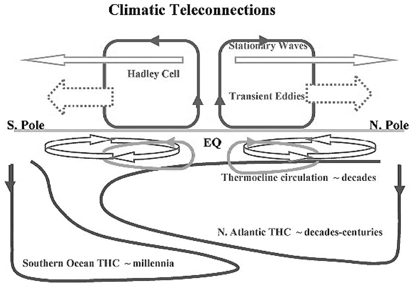
Climate mode teleconnections are statistical associations between climate variables at fixed spatial locations and the spatial pattern of climate mode anomalies that are dynamically and stochastically associated. Their origins lie with the early work by Mossman (Reference Mossman1913), Walker (Reference Walker1924) and Walker and Bliss (Reference Walker and Bliss1932, Reference Walker and Bliss1936) on statistical correlations in World Weather; the link between station weather and the SOI, NPO and NAO, and Walker’s quest to determine the basis for seasonal weather forecasting (see the modern re-evaluation of Walker’s contribution as the basis for seasonal forecasting and understanding of climate variability in Wallace, Reference Wallace2025). The fundamental physical mechanisms that underpin teleconnections between the tropics and extratropics and interhemispheric involve energy transport and wave propagation in the atmosphere and the ocean (Alexander et al., Reference Alexander2002; Liu and Alexander, Reference Liu and Alexander2007). On global scales, the Hadley circulation teleconnects weather and climate anomalies between the tropics and the extratropics, while the underlying subtropical ocean gyre transports extratropical anomalies back to the tropics. In the atmosphere, teleconnections bridge ocean regions, while oceanic teleconnections provide a tunnel between atmospheric regions (Figure 1.13). These are discussed in what follows.

Figure 1.13

Global types of climate teleconnections comprising the atmospheric bridge and oceanic tunnel pathways, as shown in Liu and Alexander.

Figure 1.13 Long description

Climatic Teleconnections Diagram. Shows atmospheric pathways including Hadley Cell, stationary waves, transient eddies, and thermocline circulation. Indicates global climate interactions between South Pole and North Pole, with time scale for thermocline circulation, North Atlantic THC, and Southern Ocean THC.

(2007, with permission from the American Geophysical Union)

1.4.2.1 Teleconnections with the Atmospheric Bridge

Atmospheric teleconnections are forced by internal atmospheric processes as well as surface ocean conditions. Tropical SST anomalies associate with ENSO produce convection anomalies that influence precipitation and vertical motion that excites atmospheric planetary waves that travel to the extratropics via the bridge. These waves produce quasi-stationary anomalies in the extratropics and constitute a robust bridge teleconnection (Liu and Alexander, Reference Liu and Alexander2007). Strong, zonally symmetric atmospheric teleconnections are produced by the Hadley circulation, while weaker teleconnections occur in the extratropical Ferrel Cell where mid-latitude storms drive a poleward eddy-driven teleconnection. Zonally asymmetric atmospheric teleconnections involve internal atmospheric processes such as the interactions between the jetstreams and the mid-latitude storm tracks and Rossby wave – eddy–mean flow interactions (Liu and Alexander, Reference Liu and Alexander2007). These asymmetric teleconnections are principally responsible for the strong regional dipole relationships that define the dominant climate modes like the ENSO, NAO, NPO, PNA and PSA. Extratropical SST and wind anomalies also drive an equatorward atmospheric bridge, but this is weaker than the poleward bridge generated by tropical SST variability.

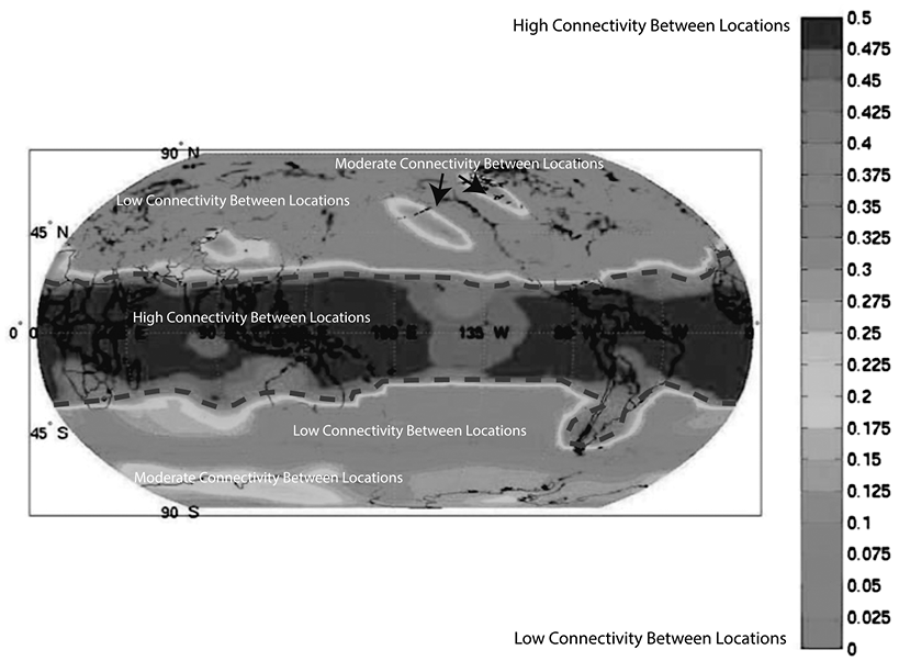
The teleconnections form network communities of nodes (Figure 1.14) and represent zones that correspond to the transition from a barotropic atmosphere (where pressure depends on density only; appropriate for the tropics–subtropics) to a baroclinic atmosphere (where pressure depends on both density and temperature; appropriate for higher latitudes) (Tsonis, Reference Tsonis and Tsonis2018). The tropics are a fully connected system due to climate signals being communicated by fast gravity waves. The extratropics are characterised by the super nodes (regions connected to many other regions) or teleconnection patterns that have been shown to act as climate stabilisers (Tsonis et al., Reference Tsonis2008; Tsonis, Reference Tsonis and Tsonis2018).

Figure 1.14

Global circulation viewed as a connected spherical network. The connectivity or teleconnections between regions are described by total number of links at each geographic location (node). This shows the fraction of the total global area that a point is connected to. The uniformity observed in the tropics indicates that each node possesses the same number of connections. This is not the case in the extratropics, where certain nodes possess more links than the rest (e.g. in the Southern Hemisphere, East Antarctica, MacRobertson Land to Wilkes Land and West Antarctica, Marie Byrd Land). The diagram is consistent with the known teleconnected regions in the climate systems described by the ENSO-IOD, PNA and PSA.

(From Tsonis, 2018, with permission from Springer International Publishing.)

Across the globe, COAs represent super nodes and form the major teleconnection patterns at the 500 hPa level. In the Northern Hemisphere, the Pacific North American (PNA) pattern is described by the super nodes in North America and Northeast Pacific Ocean (after Wallace and Gutzler, Reference Wallace and Gutzler1981). In the Southern Hemisphere, the Pacific South America (PSA) pattern is described by the super nodes over the southern tip of South America, Antarctica and South Indian Ocean (after Mo and Higgins, Reference Mo and Higgins1998). The NAO represents the extratropical network that is not connected to the tropics.

1.4.2.2 Teleconnections with the Oceanic Tunnel

The deepest oceanic tunnel of the MOC is that which transports high-latitude heat and freshwater fluxes: North Atlantic Deep Water (NADW) from the Greenland–Iceland–Norwegian Sea that outcrops at the surface in the South Atlantic and Southern Ocean and the Antarctic Bottom Water (AABW) that travels northwards along the abyssal plain to outcrop in the eastern Pacific and mid-Atlantic equatorial oceans (Schmitz, 1999a and b). The Southern Ocean determines the interhemispheric MOC because its freshwater forcing is far greater than that in the North Atlantic (this competition between NADW and AABW in driving the MOC was described by Broecker (Reference Broecker1998) as the ‘bipolar seesaw’ in ocean transport). The timescale for climate forcing in the Southern Ocean is longer than for the North Atlantic because of the absence of Kelvin waves and a western boundary current in the SO (Liu and Alexander, Reference Liu and Alexander2007). Climate signals are propagated in the surface ocean by Kelvin waves and Rossby waves at depth.

Similar to the atmospheric bridge of the Hadley circulation, the subtropical ocean cell forms an oceanic tunnel for transport of atmospheric forced mixed-layer anomalies equatorward around the gyres. Gu and Philander (Reference Gu and Philander1997) first described this oceanic tunnel as a major conduit and regulator of ocean feedback between the extratropics and the tropics. The oceanic tunnel results from the subtropical or mid-latitude temperature/salinity anomalies to be subducted from the subtropical convergence into the interior of the gyre, then propagating northwards to upwell near the equator to excite a Bjerknes feedback onto the off-equatorial atmospheric bridge (Alexander, Reference Alexander, Sun and Bryan2010). Farnetti et al. (Reference Farnetti2014) further explored the ocean tunnel mechanism via subduction in the subtropical cell driven by tradewind anomalies.

This oceanic tunnel is one mechanism that may explain the Pacific variability on decadal scales and the association between ENSO and the PDO/IPO, and the NPO/PDO and the North Pacific Gyre Oscillation (Di Lorenzo et al., Reference Di Lorenzo2008). Broadly, the distance for particle transport from the mixed layer subduction location determines the ~10–30-year feedback from the subtropical atmosphere to equatorial upwelling. Hence, the length of the oceanic tunnel has a significant impact on the pace of low-frequency macroweather variability.

1.4.2.3 Teleconnections with the Oceanic Super Gyres and Leakage

Inter-ocean basin exchanges of water masses occur at all levels in the ocean as part of the overall MOC, with the most significant being the Bering Strait, Drake Passage and the Indonesian Throughflow. However, in the SH, the subtropical South Pacific and South Indian Ocean gyres extend polewards towards the ACC to form a super-gyre from the leakage of intermediate depth water masses from the East Australian Current (EAC) Tasman Sea and the Agulhas Current (Ridgway and Dunn, Reference Ridgway and Dunn2007). This super-gyre connects the three ocean basins and is a feeder to the AMOC.

Mixed layer leakage of heat and salt anomalies from the Indonesian Throughflow and subtropical South Indian Ocean via the Agulhas Current around South Africa and into the South Atlantic Ocean teleconnects the Indian and Atlantic Oceans (Gordon, Reference Gordon1986). The Agulhas Current leakage results from mesoscale processes drive eddy transport westwards into the South Atlantic at the terminus of the Indian Ocean western boundary current, separating from the bulk retroflection eastwards in the Southern Ocean. Expansion of the tropics results in a poleward shift in the subtropical ridge and/or a poleward shift in mid-latitude westerly winds, and the subtropical front (Bard and Rickaby, Reference Bard and Rickaby2009) and/or strengthened tradewinds allow the atmospheric forcing of the Agulhas leakage (Biastoch et al., Reference Biastoch2009). Hence, the zero line of the wind stress curl allows the inter-ocean connection of the South Indian and South Atlantic Ocean gyres. The Agulhas leakage has a strong interannual and decadal-scale variability, whereby it leads the AMO variability by ~15 years (Biastoch et al., Reference Biastoch2015). Agulhas leakage has been identified as the amplifier of climate change during interglacials (Turney and Jones, Reference Turney and Jones2010) through its role in transporting warm salty water into the surface branch of the AMOC (Gordon, Reference Gordon1986) and warming the North Atlantic region.

1.4.2.4 Thermal Bipolar Seesaw

Anti-correlated bipolar climate change at the first order is produced by opposite-phase, obliquity-forced latitudinal and seasonal insolation shifts, plus the interhemispheric transport of temperature/salinity anomalies via the MOC ‘ocean tunnel’ (after Broecker, Reference Broecker1998). The spatial pattern of the modern AMO shows a strong signal in the NH but an overall bipolar structure in the Atlantic. The investigation of abrupt and rapid glacial age climate change events such as Dansgaard–Oeschger events (D-O) in the NH (Dansgaard et al., Reference Dansgaard1982) led to the discovery of an apparent interhemispheric asynchrony between the North Atlantic and rapid climate change events in the South Atlantic/Southern Ocean regions known as the Antarctic Isotope Maximum (AIM) events (Crowley, Reference Crowley1992; Blunier et al., Reference Blunier1998). The resulting thermal ‘Bipolar Seesaw’ analogy of Stocker and Johnsen (Reference Stocker and Johnsen2003) is an oceanic tunnel paradigm where North Atlantic meltwater and salinity anomalies force a shift in the meridional heat transport via the MOC to the Southern Ocean where the heat anomalies are integrated over a ~200-year period to influence Antarctic temperatures. Recent, papers have demonstrated that wind and SST changes in the Southern Ocean also force a reciprocal influence on the North Atlantic region via the MOC ‘tunnel’.

Global teleconnections during D-O and AIM events indicate that abrupt shifts in North Atlantic heat content drive latitudinal shifts in the Hadley circulation and the ITCZ into the warmer hemisphere, linking tropical climate change with that in the North Atlantic via an ‘atmospheric bridge’ (Broccoli et al., Reference Broccoli2006). Remote interhemispheric teleconnections such as between the North Atlantic and the southwest (SW) subtropical-mid-latitude Pacific are modulated by the NH atmospheric bridge, impacting the Asian monsoon and forcing a southward shift in the ITCZ. Accordingly, Chiang et al. (Reference Chiang2014) found that North Atlantic cooling (AMOC collapse) was robustly correlated with a weakening SW Pacific subtropical split jet and westerly winds, the proxy signature of which is reduced New Zealand glacial extent. More recently, Buizert et al. (Reference Buizert2018) and Markle et al. (Reference Markle2017) showed that a global ‘atmospheric bridge’ is linked to D-O events, since the Antarctic moisture sources migrate latitudinally in the SH within decades of the North Atlantic heat content. This global ‘atmospheric bridge’ arises from the latitudinal migration of the SH mid-latitude storm tracks in concert with the ITCZ migration. A comprehensive review of the oceanic and atmospheric dynamics of the AMOC is provided in Weijer et al. (Reference Weijer2019).

The underlying ‘bipolar seesaw’ hypothesis has been challenged by Pedro et al. (Reference Pedro2018) as over-simplistic. They found that (1) ‘oceanic’ heat transport is partially compensated by negative feedbacks via the ‘atmospheric bridge’ and response in the Pacific Ocean; (2) the SH heat reservoir is located in the global interior ocean to the north of the ACC, not the Southern Ocean; and (3) AIM warming events result from an increase in poleward atmospheric heat and moisture transport following sea-ice retreat and surface warming over the Southern Ocean. Skinner et al. (Reference Skinner2020) found that deep ocean convection and ventilation results in heat exchange in the Southern Ocean that modifies the sea-ice extent and the atmosphere by modulating westerly winds and Antarctic temperatures. Hence, the interhemispheric communication of abrupt climate changes during D-O and AIM events involves both the atmospheric bridge and oceanic tunnel and takes a decade or more through the atmosphere and ~200 years via the ocean (Markle et al., Reference Markle2017).

1.4.2.5 Teleconnection Non-stationarity and Implications for Paleoclimatology

There is robust evidence of global-scale teleconnections between the major centres of action or dipoles of the climate modes. However, the relatively recent discovery of ENSO flavours (canonical vs Modoki) has demonstrated that regional teleconnections may be non-stationary. Subtropical dipoles associated with the Atlantic Niño, IOD and ENSO are also non-stationary, particularly in longitude. Planetary wave modes and harmonics (discussed in Chapter 2) modulate mid to lower tropospheric atmospheric anomalies. Similarly, wind-forced shifts in the oceanic convergence, divergence and frontal zones change the oceanic tunnel pathway and similarly surface current fields and inter-basin exchanges. Hence, both the spatial and temporal associations between regionally teleconnected areas maybe non-stationary even on short timescales. Many teleconnections are the product of stochastic relationships that are non-stationary in space and time. Hence, in synoptic paleclimatology the robust approach is to examine the direct relationship with the proximal COA and treat any dynamically or statistical teleconnected relationship as non-stationary. Forced climate change also modulates the strength and dominance of the climate mode physics as well as changes the spatial representation of statistical relationships (Empirical Orthogonal Functions [EOF] for the major climate modes may explain less or more variance).

In addition, the view of climate modes and teleconnections fashioned from the anthropogenic instrumental data may be flawed when applied to the paleoclimate record. It is prudent to assume a priori that the dynamics of regional proxy-climate signals from centres of action or dipoles need to be resolved before drawing any conclusions about their relationship to climate mode phase and global implications. This is where atmospheric and surface ocean reconstructions using the synoptic paleoclimatology techniques outlined in this book, provide the framework for understanding weather-to-climate variability and climate mode phase, stationarities or non-stationarities, dynamical or stochastic forcing. The integrity of gridded paleoclimate reanalyses builds more robust time series of climate mode flavours.

1.5 Macroweather, Earth System Memory and the Proxy Climate World

The solar heating of the Earth’s atmosphere and surface drives turbulence and winds in the atmosphere that then drive ocean eddies and currents (this is the so-called heat engine). The turbulent heating of the atmosphere perturbs the planetary features such as the jetstreams, which then excite Rossby waves that propagate in the atmosphere to develop the large-scale flow that steers individual weather systems. The scaling for the onset, transition and decay of the large-scale flow is ~7–10 days (Lovejoy, Reference Lovejoy2019). In contrast, turbulent eddies in the ocean (the ocean weather) take 1–2 years to reach the planetary scale of an ocean gyre. Hence, the synoptic scale of the atmosphere (troposphere) is fast and that of the ocean is slow. Similarly, circulation in the stratosphere, tropical convection propagation across the equatorial zone and land surface heating/cooling regimes are all slower than the evolution of weather in the troposphere. The slower modes regulate the propagation and life cycle of weather and can influence tropical cyclone tracks, jetstreams and mid-latitude storm tracks (Lang et al., Reference Lang2020). Hence, weather patterns can be classified into WRs that are defined as persistent states of large-scale circulation (see Chapter 5). They are a function of natural internal variability and forced climate change boundary conditions. In general, they categorise weather into cyclonic (transient) and blocked (quasi-stationary) states and have a large influence on the likelihood of extremes that represent the transition from ‘quiescence to chaos’.

The proxy climate record that contains weather-like information such as that contained in the ice core archive, coral archive and speleothem archive has a resolution (both discrete recording potential and current analytical capability) of subseasonal at best (10–60 days) and typically of seasonal to biannual. Other records such as varved-lacustrine sediments and tree-ring records can be resolved at bi-annual to annual resolution, while glacial extent (defined by moraines, for example), and the coastal morphosedimentary record can be resolved at multi-decadal to centennial resolution. Thus, the proxy climate record contains discrete weather-like information across the subseasonal to centennial scales. This corresponds to the scaling of macroweather, a term proposed by Lovejoy and Schertzer (Reference Lovejoy and Schertzer2013) to fill the gap between weather and climate (see Lovejoy, Reference Lovejoy2019, figure 2). See recent review papers on climate variability for scales by Franzke et al. (Reference Franzke2020) and Lovejoy (Reference Lovejoy2019). The current understanding of the drivers of variability separates macroweather and climate states, and distinguishes between deterministic or dynamical atmosphere–ocean processes and pure stochastic noise. This is the fundamental difference between the ‘dynamical meteorological’ view and the ‘stochastic turbulent’ view of the coupled system (Lovejoy, Reference Lovejoy2019). Indicative time series showing the variability on weather, macroweather and climate scales is shown in Figure 1.15.

Figure 1.15

Air temperature variability for each of the weather, macroweather and climate scaling regimes driven by different non-linear climate dynamics. The scaling comparison is made for 1 hour, 20 days and 1 century as far as possible, by making the sample 720 points long (t on the x-axis); each series has its mean removed and the temperature fluctuation $\Delta T$ is normalized by its standard deviation (4.49 ± K, 2.59 ± K, 1.39 ± K, respectively), with $\Delta T/\sigma$ shown on the y-axis. The weather and macroweather series have been displaced in the vertical by four units for clarity. The most important observation of the scaling regimes is that in the weather (Haar Fluctuation $H=0.4$, increasing) and climate (Haar Fluctuation $H=0.4$, increasing) series the signal has a tendency to ‘wander’ whereas in the middle (the macroweather regime) successive fluctuations have a tendency to cancel each other out (Haar Fluctuation $H=-0.4$, decreasing). The figure was accessed from S. Lovejoy, McGill University, www.physics.mcgill.ca/~gang/reference.list.htm). See also Lovejoy (Reference Lovejoy2019).

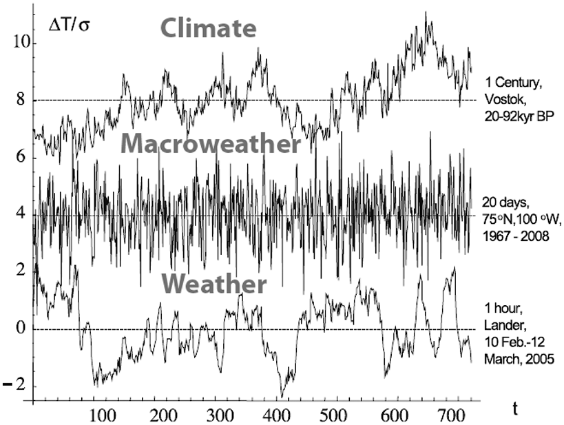
Macroweather is an averaging state (cancelling fluctuations around a zero mean) of successive 10-day weather cycles and the low-frequency internal (unforced) variability of the atmosphere–ocean system. Macroweather results from the breakup, decay or scaling of weather turbulence and represents many lifetimes of planetary structures. The average of macroweather is climate and is a window into time where the external boundary forcings are unchanged. Macroweather comprises (1) the annual cycle; (2) weather-like stochastic noise (e.g. eddy, wave and current propagation); superimposed quasi-periodic internal atmosphere–ocean oscillations that respond to stochastic and feedback forcing (e.g. ENSO and PDO); and the delayed system response to abrupt or intermittent external forcings such as volcanism or solar output variability. Low-frequency internal variability on centennial timescales has been attributed to deep ocean convection cycles such as Southern Ocean Centennial Variability (SOCV, Latif et al., Reference Latif2013) and on millennial timescales to the thermohaline circulation and the response to glacial discharge-ocean circulation feedbacks in the North Atlantic and Southern Ocean. Internal atmosphere–ocean variability is at the core of paleoclimate investigations and because it is the product of dynamical mechanisms and stochastic noise, we need to comprehensively investigate the component variances in each paleoclimate time series, for seasonal, intraannual, interanual and decadal periods.

Lovejoy’s definition of weather, macroweather and climate is that it is not scalebound (invariant) but instead is scaling and can be characterised by scaling exponents across all scales from weather to mega-climate. The statistical scale symmetries and power-law correlations of macroweather imply long climate-system memory or long-range dependence. Weather to climate fluctuations are expressed and based on the Haar fluctuation power exponent according to

$\text{Fluctuations}\sim {(\text{Interval}\Delta t)}^H\sim {(\text{Scale})}^H.$(1.2)

Haar fluctuations are the difference between the averages of the first and second halves of intervals, and they define which weather-to-climate regimes are distinguished by average fluctuations that increase with timescale $\text{(}H>0)$ and those in which they decrease with scale $\text{(}H\text{<}0)$ (Lovejoy and Schertzer, Reference Lovejoy and Schertzer2013). This can be distinguished from Gaussian ‘white noise’ that has an H exponent of –0.5. Macroweather fluctuations decrease with scale (inter-annual variability has greater magnitude than interdecadal for the same spatial scale); and at climate scale fluctuations increase (glacial–interglacial variability has greater magnitude than millennial variability).

Here H is the fluctuation power exponent, $H>0$ when fluctuations are unstable (producing a trend or wandering), and $H\text{<}0$ when fluctuations are stable or converge to an average. Typically, the ocean has $H\text{<}0$ (Lovejoy, Reference Lovejoy2019). In Figure 1.16, it can be seen that H varies with latitude and is near zero over the oceans and lower over land, typical values being –0.1 and –0.3, respectively. Hence the oceans have large memory (high hindcast/forecast skill) and shorter memory over land (low hindcast/forecast skill). Therefore, the ocean provides the most potential for both reconstructing past paleoclimate and modelling future projections at subseasonal to multi-decadal scales (see Chapter 13). However, the challenge in analysing and interpreting paleoclimate data is to remove forced low-frequency variability (such as volcanism and solar) and quasi-periodic oscillations from the stochastic macroweather signal. Spatial macroweather time series are highly intermittent (high spikiness) and multifractal, whereas temporal macroweather time series are nearly Gaussian with low intermittency (low spikiness). These characteristics can be applied to forecasting at monthly, seasonal, annual and decadal scales.

Figure 1.16

Global distribution of H exponents for macroweather: spatial distribution of the exponent H estimated at 5 × 5 resolution using monthly resolution data from the NCEP reanalyses (1948–2010) and estimated by a maximum likelihood method. The mean was –0.11 ± 0.09. H is near zero over the oceans and is lower over land, typical values being –0.1 and –0.3, respectively. Important for high temporal resolution paleoclimatology, these H values correspond to large memory (and hence hindcast skill) over oceans and lower memory and skill over land.

(From Lovejoy, 2018b.)

The transition from weather to climate scales has primarily been investigated for temperature and based upon the regional to global energy flux ε. The lifetime of planetary structures and hence the weather–macroweather transition is ${\tau }_w\approx 5–10\text{days}$, based on an $\epsilon \approx \text{1}\text{mW/kg,}L=20,000\text{km}$ (the largest great circle distance). The 10-day transition is expressed by the statistical properties of the atmospheric signal since the atmosphere is a heat engine that converts solar energy into mechanical (wind) energy (Lovejoy, Reference Lovejoy2019). When the theory is applied to the ocean (which is similarly turbulent with $\epsilon \approx {\text{10}}^{-\text{8}}\text{W/kg}$ but with a 1,000 times higher heat capacity), a transition occurs up to 40 times longer at about ${\tau }_w\approx 1–2\text{years}$, and up to ${\tau }_w\approx 3–4\text{years}$ for the tropical oceans (Lovejoy, Reference Lovejoy and Tsonis2018). The estimated transition between scales ${\tau }_w$ using precipitation varies somewhat with latitude from about 2 to 5 days, which is a little less than for the temperature (5–10 days) (Lovejoy and Schertzer, Reference Lovejoy and Schertzer2013; de Lima and Lovejoy, Reference de Lima and Lovejoy2015). The weather–macroweather transition is $\text{(}{\tau }_w\approx 10\text{days)}$.

Over land, consecutive values of macroweather (e.g. temperature) tend to cancel out, whereas over the ocean the temperature is more persistent and the anomalies change sign only after several time steps in Haar fluctuation analysis. Hence, the longer ocean weather–ocean macroweather transition corresponds to lifetimes of large-scale ocean gyres (and other structures) that live much longer than atmospheric structures (Lovejoy and Schertzer, Reference Lovejoy and Schertzer2013).

Macroweather is the dynamical regime of fluctuations with timescales between the lifetimes of planetary structures $({\tau }_w)$ and the climate regime where either new (slow) internal processes or external forcings begin to dominate $\text{(}{\tau }_c\text{)}$ (Lovejoy et al., Reference Lovejoy and Tsonis2018). The true climate regime begins at ${\tau }_c\approx 10\text{or}30\text{years}$ in the Anthropocene, and ${\tau }_c\approx \ge 100\text{years}$ in the pre-industrial epoch, although ${\tau }_c$ is highly uncertain over the Holocene. The recognition of slow climate and fast macroweather scales is an important basis for reducing a paleoclimate time series into two components: (1) signal of the macroweather response to changes in climate boundary conditions (such as those that are orbitally forced) and (2) signal of the response due to the internal variability (dynamic and stochastic). Climate stability has been redefined into the length of the macroweather-to-climate transition scale. Lovejoy and Lambert (Reference Lovejoy and Lambert2019) analysed the EPICA Dome C ice core dust flux time series for the past 800,000 years. They resolved that interglacials and glacial maxima experienced exceptionally stable climate with a large macroweather-to-climate transition scale, ${\tau }_c$ (~2 ka), compared to unstable mid-glacial phases with a ${\tau }_c$ of 300 years. The latter observations accord with ice-age abrupt climate changes associated with D-O and Heinrich events. The Holocene has had a very large ${\tau }_c$ of ~7.9 kyr that is approaching the half-orbital precession cycle, with a known strong forcing of interhemispheric seasonality strength.

Important for synoptic paleoclimatology is the fact that at the macroweather scale, atmospheric processes and changes in the hydrological cycles are the main drivers of variability (Lovejoy and Lambert, Reference Lovejoy and Lambert2019). Stable climate during interglacials, glacial maxima and glacial inceptions is characterised by low drift, moderate intermittency and strong extremes (spikiness). In other words, stable atmospheric conditions are punctuated by strong extreme events such as flood and drought. With unstable climate during mid-glacials, where boundary conditions are changing, the atmosphere is characterised by high drift, weak intermittency and weak extremes. Hence, long (short) macroweather scales are characterised by strong (weak) extremes; for example, the Holocene paleoclimate archive should be punctuated by strong flood and drought regimes that are represented in spatial and temporal time series as high intermittency of spikiness.

Lovejoy (Reference Lovejoy2019) calculated macroweather scaling as 10 days to >100 years (for pre-1850 CE industrialisation) and 10 days to ~30 years (for post-1850 CE industrialisation), since the recent anthropogenic climate change signal emerges above natural variability after 30 years. At its highest frequency, macroweather comprises monthly weather averages that correspond to two planetary weather cycles (Lovejoy, Reference Lovejoy2019), which is comparable to the quasi-monthly resolution of the proxy climate archive. Autocorrelation in macroweather fluctuations represents the memory in the atmospheric-ocean system including large-scale flow (transient and blocking), storm tracks, mesoscale ocean eddies, tropical convection locations, and land surface and ocean heat storage. It is this ‘macroweather memory’ that the proxy climate archive is recording: that is, glacial memory, land-surface memory, coastal memory, ice-sheet memory and ocean thermocline memory. The macroweather scaling is slightly different for latitudinal zones and between hemispheres because of the difference in weather-ocean turbulence between land-ocean area and tropical versus extratropical regions. Southern Hemisphere climate proxies would have the greatest reliability in preserving the macroweather signal due to the 60% ocean cover. An example of characteristics of atmospheric phenomena and macroweather circulation for the Northern Hemisphere is shown in Figure 1.17.

Figure 1.17

Characteristics and interactions between large-scale atmosphere–ocean circulation and ocean and land memory that lead to macroweather variability for the Northern Hemisphere.

(Adapted from Lang et al., 2020, with permission from the American Geophysical Union.)

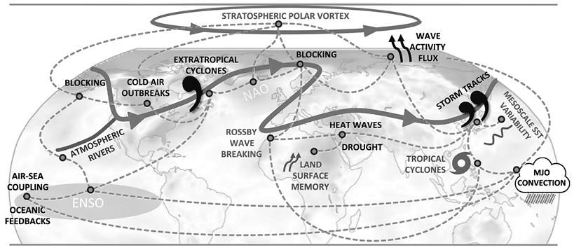
Macroweather states can be used to define clustered, stochastic, weather-like anomalies in paleoclimate records and are hence a departure from the large-scale atmospheric and ocean flow. Macroweather has flavours depending upon the dominance of internal climate modes at monthly to interannual timescales (e.g. ENSO and NAO) and decadal timescales NAM and SAM (after Franzke, Reference Franzke2009; see Section 1.4 for the definition of climate modes), and transitional macroweather between climate modes. The temporal accordance between macroweather and the higher-resolution natural archive highlights why spatial paleoclimate reconstructions display weather-like characteristics or ‘imprints’ of large-scale circulation such as mid-latitude storm tracks, in addition to shifts in global circulation features such as cloud convergence zones, and subtropical anticyclone and extratropical oceanic cyclone COA.

The scalebound view requires that every power of 10 scale requires a new mechanism or law to explain variability and forces paleoclimate investigations to fit spectra to processes or modes. In contrast, self-similar scaling produces similarity at all scales by zooming up and down scale under the same physical laws and principles (known as fractal scaling; see Lovejoy, Reference Lovejoy2019), such that an eddy squall can be scaled to a low pressure system. This is important for paleoclimate process models scaling up to explain regional macroweather variability, or deconvolution to dynamic and stochastic contributions. In the morpho-sedimentary record, cascading scales have been identified, particularly in fluvial, hydrological and coastal environments, for example, the coastal tract approach uses self-similar scaling processes from a sand ripple to the shoreface (Cowell et al., Reference Cowell2003).

A high-level challenge for synoptic paleoclimatology is to reconstruct natural climate variability during the pre-industrial period because our modern observations reflect the anthropogenic ‘slowing of the climate system’ and a reduction in ${\tau }_c$ from a few hundred years to a decade (Lovejoy, Reference Lovejoy2019). However, from pre-industrial through the Late Holocene, macroweather types depend upon whether they are partially forced by random volcanism and solar output variability. Arguably, macroweather during the past millennium (1000–1850 CE) is impacted by a high frequency of explosive volcanism events together with minima in solar output. Lovejoy and Varotsos (Reference Lovejoy and Varotsos2016) found that the solar forcing was small at annual scales and generally increased with scale, whereas volcanic forcing was very strong at annual scales but rapidly decreased, with the two becoming roughly equal after about 200 years. In addition, volcanic intermittency was much stronger than solar intermittency between 1000 and 1850 CE, and hence should produce high spikiness in millennial proxy records.

These results were challenged by Rypdal and Rypdal (Reference Rypdal and Rypdal2016), who suggest that the Little Ice Age is explained as mainly due to volcanic cooling or as a long-memory response to a strong radiative disequilibrium during the Medieval Climate Anomaly and should not be attributed to low solar activity during the Maunder Minimum. The combined work on scaling regimes and linear/non-linear responses to climate forcing presents paleoclimatologists with two paradigms to at least consider when interpreting the archive. The scaling paradigm extends the turbulence framework to encompass the dynamics of the entire climate system across scales with responses that are close to power laws. Alternatively, the dynamic paradigm treats the climate as a high-dimensional dynamical system residing in non-equilibrium stationary states, invoking response theory of non-equilibrium statistical mechanics (Rypdal and Rypdal, Reference Rypdal and Rypdal2016).

Modes of climate variability such as ENSO are considered non-linear modes of the climate system (they deviate from the scaling laws such that fluctuations on the timescales of a few years are larger than what could be expected from a scaling model), and such internal variability can be influenced non-linearly by external forces such as volcanism and solar output and lagged due to the thermal inertia of the ocean (Rypdal and Rypdal, Reference Rypdal and Rypdal2016). Quaternary examples such as D-O cycles, also known as rapid climate change events between stadial and interstadial climate in the North Atlantic region have much larger millennial-scale fluctuations than what can be expected from a 1/f description of climate noise (Rypdal and Rypdal, Reference Rypdal and Rypdal2016; Hebert et al., Reference Hebert2022). The D-O events are part of the natural variability and not externally forced, and they contribute to relatively longer persistence time and stronger non-linearities in the glacial climate (Shao and Ditlevsen, Reference Shao and Ditlevsen2016). The impact of volcanic and solar forcing together with low frequency (decadal- to centennial-scale) quasi-oscillations or long memory in the internal dynamics, means that it is prudent to test for heterogeneity between centennial periods in the natural archive if we are to understand the associated synoptic states (see Chapter 13).

1.6 The Way Forward and Scope of the Book

Modern climate analogues provide a basis for assessing the departure of past climates from our own human experience. Hence, an understanding of modern circulation at the global, large (hemispheric) and synoptic (continental-ocean basin) scales is essential for a dynamic interpretation of past climate changes. A paleoclimate record includes up to three levels of information about the weather-climate system. First-order information is recorded about the interaction of local-scale or microclimate processes with regional weather frequency defined by synoptic-scale patterns. Second-order information is recorded about the variability and persistence of the large-scale macroweather and climate modes in the atmosphere and ocean, such as storm tracks or ocean currents. The variability ranges from seasons to centennial and is subject to internal system dynamics and teleconnection stationarities. Third-order information is recorded about changes in the mean state of the climate system. These are the externally forced climate changes or responses to volcanism or solar output and planetary scale feedbacks such as ice sheet growth and decay, albedo, water vapour and land cover changes.

The challenge for paleoclimatology is to separate the three orders of information that the proxy record may contain. The main theme for the book is that synoptic reconstruction using multi-proxies allows a spatial framework to decompose the climate signal from macroweather noise, and the coupled atmosphere–ocean drivers of the macroweather and low-frequency signals, such that the paleoclimate record can be applied to forecasting and projecting from the sub-seasonal to centennial scale. The book’s aim is to provide a detailed treatment of the theory and application of synoptic paleoclimatology to the study of weather–climate evolution. While it has become common in the past few decades to see synoptic circulation patterns on weather and macroweather scales as key to understanding climatology, the study of past atmospheric circulation has received less attention in the study of paleoclimatology. The book has its origins in almost four decades of researching and teaching synoptic climatology and paleoclimatology, through the prism of the paleoclimate archive, particularly coastal morphosedimentary records, glacial mass balance and geological records, ice core glaciochemistry and isotope records, coral geochemistry and reef morphosedimentary records, aeolian dust and lacustrine sedimentary records, and marine sedimentary records. The book is structured as follows.

The Global atmospheric circulation and energy budget, together with the modern heat budget, air temperature, sea-surface temperature, sea-ice cover, moisture budget and cloud cover fields, are presented in Chapter 2. This forms the basis for the study of large-scale to synoptic scale circulation, modes and regimes. Part II focuses on the large-scale to synoptic scale atmospheric circulation (Chapter 3) and the regional wind and wave climate and ocean circulation (Chapter 4). These chapters cover the circulation and characteristics that we seek to reconstruct in paleoclimatology. The dynamics of atmospheric and ocean processes and the resulting circulation are treated largely in descriptive terms. I have chosen to present the material in this way so that the dynamics can be assessable to field-observational paleoclimatology students and paleoclimatologists first and numerical modellers second. Chapter 5 is on synoptic signatures of macroweather regimes and climate modes, where the WR or synoptic typing approaches are applied to the centres of action for each of the major regional climate modes. The synoptic tying approach underpins paleoclimate reconstructions. Part III focuses on the natural archive of proxy macroweather and climate data. Here, the approach is to define the primary archives of past large-scale to synoptic-scale atmosphere–ocean circulation, and to describe the methods and approaches to transform macroweather/climate impact to the atmospheric and ocean ‘synoptic’ attributes and dynamics. The paleoclimate archive has broadened significantly with new geochemical proxies from the terrestrial, marine and cryospheric environments, this book focuses on the primary sources of paleo-circulation: paleo-air and water masses; winds and waves; currents; storm tracks; and extreme events. The coastal archive of ocean wave, marine wind and storm climate is investigated in Chapter 6, and the tropical–subtropical marine archive of sea surface, sea-level and ocean circulation, and paleoweather in Chapter 7. The glacial archive of atmospheric circulation change is investigated in Chapter 8, and the glacier-weather regime relationships and glacial history in Chapter 9. The ice core archive of circumAntarctic atmospheric circulation change, hydroclimate and polar weather regimes are presented in Chapter 10. The aerosol tracer archive, paleo-wind fields and polar paleoweather regimes are presented in Chapter 11. Part IV of the book is focused on synoptic paleoclimate reconstruction and applications. Chapter 12 investigates the paleoclimate and proxy databases, data-assimilation and modelling approaches applied to the reconstruction of gridded paleoclimate reanalyses. Chapter 13 presents recent paleoclimate data-assimilation reconstructions and advances in defining large-scale circulation evolution and WR. It provides examples of paleoclimate reconstructions for warm climate, with a focus on the Holocene and the MIS5 period. Chapter 13 provides a forward view of assimilating synoptic paleoclimatology into climate science approaches: such as resolving future problem climates with regional weather regime knowledge and causal networks.