


Impact Statement
The indoor environment poses health challenges due to various sources of pollutants, such as volatile organic compounds and particulate matter, and could be life threatening in cases such as potential gas leaks and airborne transmission of infectious diseases. In such scenarios, cross-ventilation could play a crucial role in dispersing indoor pollutants through the exchange of indoor and outdoor air and thus minimizing the concentration of harmful substances. To understand the pollutant transport mechanisms in such scenarios, we experimentally investigate a flow through a scaled-down hollow building, immersed in an atmospheric turbulent boundary, with a pollutant source inside. The focus has been on characterizing the scalar transport through simultaneous scalar and flow measurements. The present simplified study will enable us to better understand the intricacies of scalar transport within indoor and across indoor–outdoor environments and build useful models, helping better design indoor spaces for a healthier and sustainable urban habitat.
1. Introduction
In urban environments, pollutants can emanate from both indoor and outdoor sources, posing a threat to human health, as noted in many review articles (Reference WallaceWallace 1996; Reference HannaHanna 2003; Reference Geiss, Tirenti, Bernasconi, Barrero, Gotti, Cimino-Reale, Casati, Marafante, Sarigiannis and KotziasGeiss et al. 2008; Reference Blake and WentworthBlake & Wentworth 2023; Reference MulcahyMulcahy 2023). Numerous studies have focused on modelling indoor pollutant dispersion, with a particular emphasis on flow patterns and pollutant spread in indoor spaces (Reference Holmberg and LiHolmberg & Li 1998; Reference Zhang and ChenZhang & Chen 2006; Reference Van Hooff, Blocken, Defraeye, Carmeliet and Van HeijstVan Hooff et al. 2012; Reference Blocken, Tominaga and StathopoulosBlocken, Tominaga & Stathopoulos 2013; Reference Lim, Foat, Parker and VanderwelLim et al. 2024), for example, studies on the exchange of dispersion between different indoor spaces due to natural ventilation (Reference Liu and ZhaiLiu & Zhai 2007; Reference Ai and MakAi & Mak 2015, Reference Ai and Mak2016), and then dispersion of tracer gases in agricultural settings such as greenhouses or livestock buildings (Reference Bartzanas, Boulard and KittasBartzanas, Boulard & Kittas 2004; Reference Norton, Grant, Fallon and SunNorton et al. 2009). A large number of studies (Reference Finnegan, Pickering and BurgeFinnegan, Pickering & Burge 1984; Reference Karava, Stathopoulos and AthienitisKarava, Stathopoulos & Athienitis 2007, Reference Karava, Stathopoulos and Athienitis2011; Reference Tablada, De Troyer, Blocken, Carmeliet and VerschureTablada et al. 2009; Reference Van Hooff and BlockenVan Hooff & Blocken 2010a) emphasized the critical role of cross-ventilation for ensuring a sustainable and healthy indoor environment. In such scenarios, the ventilation could be driven by (forced) wind or buoyancy or by a combination of both (Reference LindenLinden 1999; Reference Li and DelsanteLi & Delsante 2001; Reference Reichrath and DaviesReichrath & Davies 2002; Reference ChenChen 2009; Reference Ohba and LunOhba & Lun 2010). Over the last few decades, research on natural ventilation has encompassed experiments (Reference Kato, Murakami, Mochida, Akabayashi and TominagaKato et al. 1992; Reference Karava, Stathopoulos and AthienitisKarava et al. 2011), analytical models (Reference Li and DelsanteLi & Delsante 2001; Reference Costola, Blocken and HensenCostola, Blocken & Hensen 2009) and simulations (Reference Jiang, Alexander, Jenkins, Arthur and ChenJiang et al. 2003; Reference Van Hooff and BlockenVan Hooff & Blocken 2010b; Reference Kosutova, Van Hooff, Vanderwel, Blocken and HensenKosutova et al. 2019). Despite the extensive body of work on dispersion in indoor environments, there is a noticeable gap in the literature concerning investigations into cross-ventilation coupled with indoor dispersion sources. To bridge this gap, the present study experimentally explores a scenario involving the flow through a scaled-down hollow building (a cube) with windows positioned upstream and downstream. This set-up is submerged within a rough-wall turbulent boundary layer inside a water-tunnel facility, and a pollutant (scalar) source is introduced within the hollow cube, as depicted in figure 1.
Schematic showing the side view of the experimental arrangements used in the present study. The hollow (cubic) building with openings upstream and downstream was immersed in a rough-wall turbulent boundary layer, mimicking the flow through a hollow building in an atmospheric boundary layer condition. The cube was affixed on the false floor set-up mounted on the glass floor of the flume test section. The cube faced an incoming rough-wall boundary layer obtained using a series of roughness blocks mounted on the false floor far upstream of the test section. A scalar (dye) source was flush mounted on the building's floor, facilitating dye injection, essentially representing a pollutant source. Simultaneous PLIF and PIV measurements were performed in the streamwise centre plane ( $x$–
$x$– $y$ plane) along the building centre and the source, to capture the scalar concentration and velocity fields, respectively.

It is well known that the placement of windows relative to the building's floor is a critical parameter governing the flow patterns within the building and, hence, would influence the ventilation performance, as reported in a number of studies (Reference MeroneyMeroney 2009; Reference Ramponi and BlockenRamponi & Blocken 2012; Reference Bangalee, Miau, Lin and FerdowsBangalee et al. 2014; Reference Perén, Van Hooff, Leite and BlockenPerén et al. 2015; Reference Kasim, Zaki, Ali, Ikegaya and RazakKasim et al. 2016; Reference Tominaga and BlockenTominaga & Blocken 2016; Reference Kosutova, Van Hooff, Vanderwel, Blocken and HensenKosutova et al. 2019). However, it is worth noting that these studies, while providing valuable information shedding light on flow patterns and turbulence statistics, notably lack the exchange of scalar across indoor and outdoor environments, as was also noted by Reference Tominaga and BlockenTominaga & Blocken (2016). They conducted experimental measurements of flow and dispersion in a wind tunnel to study cross-ventilation through a hollow cube with high aspect ratio ( ${\rm width/height}=3$) openings on opposite sides, facing the windward and leeward facades, and with a scalar source within the building. They found that altering the window positions significantly affects both the time-averaged indoor pollutant concentration and its flushing efficiency. They also observed that the air exchange rate in such configurations may not be the most reliable indicator of ventilation efficiency; instead, the window position relative to the pollutant source is crucial. More recently, Reference Kosutova, Van Hooff, Vanderwel, Blocken and HensenKosutova et al. (2019) conducted wind-tunnel experiments and computational fluid dynamics (CFD) simulations to investigate natural cross-ventilation through a hollow isolated cube with various window positions, similar to the model used by Reference Tominaga and BlockenTominaga & Blocken (2016) but with louvres installed on the windows. They reported that the impact of louvres on various critical parameters related to ventilation, such as the airflow pattern, age of air and air exchange efficiency, would vary depending on the window positions. The qualitative measurements by Reference Tominaga and BlockenTominaga & Blocken (2016) of scalar exchange across indoor–outdoor have provided valuable insights into scalar transport in cross-ventilating flows. However, it is worth noting that a further comprehensive understanding of scalar transport mechanisms requires simultaneous quantitative measurements of both the flow field and scalar quantities.
Bridging this gap, the present work performs simultaneous planar laser-induced fluorescence (PLIF) and particle image velocimetry (PIV) measurements, investigating a flow through a hollow cube, with windows upstream and downstream, submerged inside a rough-wall (water) turbulent boundary layer. The model has an arrangement of scalar (Rhodamine 6G dye) injection into the cube from the centre of the bottom floor, as shown in figure 1. The present work builds upon the qualitative investigation of Reference Tominaga and BlockenTominaga & Blocken (2016) on flow and dispersion, using a similar configuration. The present focus has been on understanding the transport of a passive scalar, characterized by the mean and transient behaviours, quantified using simultaneous PLIF and PIV measurements, with the former quantifying the scalar and the latter capturing the flow field information within the cube. These measurements are conducted at three incoming flow Reynolds numbers ( $Re=U_{Ref}H/\nu =20\ 000$, 35 000 and 50 000) for three window positions, as ‘centre’, ‘up-down’ and ‘down-up’, as shown in figure 2(a–c); here, $U_{Ref}$ is the incoming flow streamwise velocity at the cube height, $H$, measured without the cube, and $\nu$ is the kinematic viscosity of water. To the best of our knowledge, this paper represents the first comprehensive analysis of simultaneous flow and dispersion processes within a cross-ventilated generic building configuration.
Schematics showing the three-dimensional view of the hollow building models used for the present study: (a) centre, (b) up-down and (c) down-up configurations. The flow is from left to right, and the dye is injected from a 5 mm hole flush mounted at the centre of the floor of the model ( $x,y,z=0,0,0$), as indicated in red. All the units shown are in mm.

The layout of the article is as follows. Section 2 presents the experimental methodologies followed by § 3 showing the results on the effects of window position on scalar transport. Finally, a broad summary and conclusions are provided in § 4.
2. Experimental methods
2.1 Building models
The model building in the present work is a transparent hollow acrylic cube having an outer dimension ( $H$) of 100 mm and a wall thickness of 8 mm, as depicted in figure 2(a). The cube had two opposite openings (windows), one in the windward and the other in the leeward facade, with both of the openings being of similar size, of $35 \times 35$ mm, yielding a facade porosity of approximately 10 %, akin to the configuration by Reference Kosutova, Van Hooff, Vanderwel, Blocken and HensenKosutova et al. (2019). It may be noted that realistic building designs typically incorporate multiple smaller windows rather than a single large one. Nevertheless, in the present study, a simplified approach featuring a single large opening has been adopted to keep the indoor flow relatively simple, thus helping better understand both flow patterns and the scalar transport mechanisms.
This scale of the present model, compared with an average UK single-storey building, is in the range of 30 : 1 to 45 : 1, similar to previous studies (Reference Richards, Hoxey, Connell and LanderRichards et al. 2007; Reference Biswas and VanderwelBiswas & Vanderwel 2024; Reference Lim, Foat, Parker and VanderwelLim et al. 2024). In total, three window configurations were studied: (a) ‘centre’ with openings at the centre of the windward and leeward facades, (b) ‘Up-down’ with the upstream opening positioned closer to the roof of the cube and the downstream window near the ground and (c) ‘Down-up’ with the upstream opening closer to the ground and the downstream window near the roof. In each of these configurations, the dye was injected from the centre of the bottom floor of the building, as also indicated in the figures.
The present focus is to understand the effects of window position on indoor pollutant transport in cross-ventilating flow conditions closer to realistic urban boundary layer conditions where varying window height would bring changes in the oncoming flow at the window level. Therefore, different window positions are compared while the Reynolds number based on a fixed reference velocity ( $U_{Ref}$, measured without the model) is kept constant, which would ensure uniformity and consistency in analysis across different wind positions, similar to previous studies on cross-ventilations (e.g. Reference Tominaga and BlockenTominaga & Blocken 2016; Reference Van Hooff, Blocken and TominagaVan Hooff, Blocken & Tominaga 2017; Reference Kosutova, Van Hooff, Vanderwel, Blocken and HensenKosutova et al. 2019). The alteration in the positions of the openings across these configurations led to significant variations in the flow patterns within the cube, consequently resulting in substantial differences in scalar transport and distribution within, as will be discussed in § 3.
2.2 Water-tunnel set-up
The current experiments were performed inside the water-tunnel facility at the University of Southampton, having a test section 8.1 m in length, 1.2 m in width and 0.9 m in height. The water depth was maintained to be around 0.6 m throughout the experiments. The hollow cube was mounted on the false floor placed on the test section's glass floor. Upstream to the test section, a series of roughness blocks (cubes) of varying sizes (30 to 8 mm) were mounted on the false floor, as shown in figure 1, producing a nearly fully developed rough-wall turbulent boundary later in the test section downstream, mimicking an atmospheric boundary layer condition (similar to Reference Lim, Hertwig, Grylls, Gough, Van Reeuwijk, Grimmond and VanderwelLim et al. 2022; Reference Rich and VanderwelRich & Vanderwel 2024). The present experiments were conducted at three building height-based Reynolds numbers ( $Re=U_{Ref}H/\nu$) of $\approx$20 000, 35 000 and 50 000, and the corresponding streamwise velocities at the cube height ( $U_{Ref}$) were approximately 0.18 m s $^{-1}$, 0.32 m s $^{-1}$ and 0.45 m s $^{-1}$, respectively; here, $U_{Ref}$ was measured at the cube height with no cube in the test section and $\nu$ is the kinematic viscosity $=0.89\ {\rm mm}^2\ {\rm s}^{-1}$, at a water temperature of $25 \pm 1\,^\circ$C.
2.2.1 The PIV and PLIF measurements
We are interested in two-dimensional maps of the velocity and scalar fields within the cube, captured simultaneously through PIV and PLIF measurements, in the streamwise symmetric plane ( $x$–
$x$– $y$) along the centre line of the building and also aligned with the source location, as shown in figure 1. The illumination was provided using a 100 mJ Nd:YAG double-pulsed laser emitting light at a wavelength of 532 nm. Two cameras had appropriate filters to distinguish the PIV and PLIF signals. The laser beam, originating from the double-pulsed YAG laser, passed through a converging–diverging lens, generating a light sheet that traversed through an acrylic sheet, which was partially submerged at the free surface. This acrylic sheet was employed to mitigate the waviness of the free surface in the flume. For PIV measurements, the flow was seeded with 50 $\mathrm {\mu }$m polyamide particles and circulated in the flume until the desired density and a nearly uniform particle distribution were achieved. The flow field, illuminated at a frequency of 10 Hz, was captured at a spatial resolution of 0.18 mm pixel $^{-1}$ by a Lavison Imager MX 4M camera with a resolution of $2048 \times 2048$ pixels. To ensure convergence of time-averaged statistics, 2000 pairs of images were processed in Davis 10, employing a 4-pass interrogation window ranging from $128 \times 128$ down to $24 \times 24$ with a 50 % overlap to ensure a high correlation (refer to Reference Lim and VanderwelLim & Vanderwel (2023) for additional details on PIV processing).
The experimental set-up facilitated the injection of a neutrally buoyant solution of Rhodamine 6G fluorescent dye at the floor of the cube, essentially replicating a ground-level point source of a passive scalar (pollutant) with negligible effects on the flow (similar to Reference Lim and VanderwelLim & Vanderwel 2023). The dye with concentrations ( $C_S$) of 1 mg l $^{-1}$ was injected at a constant flow rate ( $Q_S$) 7 cc min $^{-1}$, using a needle valve and a Mariotte bottle, ensuring a minimal disturbance to the flow. It may be noted that, due to the extremely low concentration of Rhodamine 6G, the density of the dye solution is approximately 0.001 % higher compared with freshwater, indicating it to be neutrally buoyant. The dye source was connected with a thin tube, which was further connected to an internal channel in the acrylic false floor. This finally facilitated dye injection into the cube through a hole (perpendicular to the floor) situated at the centre of the cube's floor (see figures 1 and 2). The hole had a diameter of 5 mm, and the aqueous dye solution was injected into the cube at a velocity of approximately 5.9 mm sec $^{-1}$. The ratio of this velocity of injection of the dye solution from the source to the streamwise velocity measured closer to the wall (at $x/H,y/H,z/H=0$,0.05,0) is approximately 0.2, which is fairly small and hence would not be expected to have any considerable effects on the indoor flow. To further ensure this, the indoor streamwise velocity obtained with the source off is compared with the one obtained with the source on, and they are found to be nearly identical, thus ensuring it to be a passive injection. Also can be noted is that the speed of the injection from the source is even much lower than $U_{Ref}$, with their ratio being approximately 0.03, significantly lower than previous studies, for example, the 0.25 ratio reported by Reference Tominaga and BlockenTominaga & Blocken (2016). The dye Schmidt number was ${\approx }2500\pm 300$, indicating a much higher momentum diffusion rate than the scalar (Reference Vanderwel and TavoularisVanderwel & Tavoularis 2014). The absorption and emission peaks of Rhodamine 6G are at 525 and 554 nm, respectively. To eliminate incident light from the laser and reflected light from the PIV particles, an optical long-pass filter with a sharp cutoff at 540 nm was employed. This filter was positioned in front of the 5.4 MP 16-bit depth sCMOS camera, which recorded the fluorescence emitted by the excited dye at a spatial resolution of 0.082 mm pixel $^{-1}$. It can be noted that the flume water quality was continuously monitored, ensuring no residual dye build-up over time and no potential impact on the accuracy of PLIF measurements.
The local dye concentration ( $C$) was determined from the fluorescence intensity following a calibration procedure and the methodology is described here in a much more succinct way, and the details can be found in the recent study by Reference Lim, Hertwig, Grylls, Gough, Van Reeuwijk, Grimmond and VanderwelLim et al. (2022). The processing began with the calibration, performed using two thin glass tanks filled with known concentrations of Rhodamine 6G dye (0.03 and 0.05 mg l $^{-1}$), which was already validated as in the linear response regime (Reference Vanderwel and TavoularisVanderwel & Tavoularis 2014; Reference Lim, Hertwig, Grylls, Gough, Van Reeuwijk, Grimmond and VanderwelLim et al. 2022). This was followed by a post-processed linear mapping of the fluorescence intensity measured at each pixel to the local dye concentration. The dye accumulation in the recirculating water tunnel was minimal due to the tank's substantial total volume of approximately 30 000 litres and also due to the overnight chlorine treatment breaking down any dye build-up. Nevertheless, the background dye levels were diligently monitored before and after experiments and duly considered in the calibration process. During the measurements, the temporal variations in the laser pulse were recorded using an energy monitor and then accounted for in the post-processing. The simultaneously measured velocity and concentration fields were mapped into a unified coordinate system, enabling us to calculate the joint velocity–concentration statistics, with measurement uncertainty for the joint statistics below 10 %.
2.2.2 Characterization of boundary layer
Before beginning experiments involving the cube, the incoming flow was characterized in terms of the boundary layer properties without the model in the test section. In figure 3, the wall-normal ( $y/H$) profile of the mean streamwise velocity ( $\bar {U}/U_{Ref}$), the Reynolds stress ( $-\overline {u^{\prime }v^{\prime }}$/ $U^2_{Ref}$) and velocity profile in linear–logarithmic scale ( $u^{+}$ vs. $y^{+}$) are shown; here, $\bar {U}=$ mean streamwise velocity, $u^{\prime }=$ streamwise fluctuating velocity, $v^{\prime }=$ wall-normal fluctuating velocity, $u^{+}= \bar {U}/{u_{\tau }}$ and $y^{+}=$ wall-normal co-ordinate= $yu_{\tau }/\nu$. Presently, the friction velocity ( $u_{\tau }$) was estimated following the total stress method (Reference WalkerWalker 2014) from the square root of the peak of the Reynolds shear stress in figure 3(a(ii),b(ii),c(ii)). It can be noted that the friction Reynolds numbers, defined here as $Re_{\tau }=u_{\tau }H/\nu$, were approximately 2300, 2600 and 3500 in the $Re$ cases studied.
Characterization of the incoming flow at  $Re$ of (a) 20 000, (b) 35 000 and (c) 50 000, in terms of the wall-normal ( $y/H$; $H=$ cube height) profiles of the: (i) normalized mean streamwise velocity ( $\bar {U}/U_{Ref}$); (ii) normalized Reynolds stress ( $-\overline {u^{\prime }v^{\prime }}/U^2_{Ref}$); and (iii) velocity in linear–logarithmic scale ( $u^{+}$ vs. $y^{+}$). These measurements for the base flow were taken in the water-tunnel test section without the cube.

2.3 Analytical model
In the present work, the experimental measurements are further aided by calculating the concentration from ‘box model’, a mass balance-based model employed for predicting air quality in urban settings (Reference LettauLettau 1970; Reference Hanna, Briggs and HoskerHanna, Briggs & Hosker 1982). Before we provide a brief outline of the model, it is first worth noting that our indoor dispersion flow procedure involves distinct stages (‘I’ to ‘V’), as illustrated in figure 4(a), depicting the spatially averaged concentration ( $C$) with time ( $t$). In the figure, the (statistically) steady-state concentration in the stage ‘III’ is reached following an initial no dye injection stage ‘I’, and a scalar build-up stage ‘II’ spanning from the beginning of scalar injection at $t_{01}$ up to the time to reach a statistically steady equilibrium concentration. Moving further in time, stage ‘III’ finishes as the scalar source is shut ( $C_S=0$) at $t_{02}$, resulting in an exponential decay in the scalar concentration in stage ‘IV’, and then the onset of stage ‘V’ after the scalar is entirely flushed out of the cube.
(a) Schematic representing the typical profile of spatially averaged concentration within the cube against time and the respective stages involved. (b) Schematic represents the ‘box model’ along with the input parameters.

To begin with the model, figure 4(b) illustrates the important mass fluxes in the ‘box model’ in the current flow scenario, depicting a cube with windows at its upstream and downstream faces. The cube is assumed to experience a uniform advective inflow and outflow and a source emission from the centre of the floor. In the model, we have (from experiments) the geometric input parameters such as the control volume (CV) inside the box,  $V_m=lwh$, where, ‘ $l$’, ‘ $w$’ and ‘ $h$’ are the length, width and height of the CV, respectively, and $A_o$ ( $=w_oh_o$) is the opening area where ‘ $w_o$’ and ‘ $h_o$’ are the window width and height, respectively. Additional input parameters include the inflow velocity ‘ $U_i$’, outflow velocity ‘ $U_o$’, inflow scalar concentration ‘ ${C_i}$’, scalar concentration at the exit window ‘ ${C_o}$’, injected scalar strength ‘ $C_S$’ (in mg l $^{-1}$) and volume flow rate of aqueous-scalar solution injected ‘ $Q_S$’ (in mm $^3$ sec $^{-1}$). It may be noted that the flow speeds at the window levels are different for the three window configurations and are taken from the experimental measurements to account for in the model. By applying the scalar mass balance (see (
) below), we can derive from the model the rate of change of the spatial average of the scalar concentration within the cube ( $C$) as

It is important to highlight that the model operates under the assumption of perfect mixing, where the injected scalar uniformly mixes (instantaneously) across the cube's entire CV, a condition not reflective of practical scenarios. Moreover, the model assumes that the indoor concentration ( $C$) is equivalent to the exit concentration ( $C_o$), whereas recent measurements show their ratio, $\alpha =C_{o}/C\neq 1$, as we will discuss later in § 3.3. To align the model with the practical scenario, we introduce a mixedness factor ‘ $\beta$’ and the indoor-to-exit (in a mean sense) concentration ratio ‘ $\alpha$’ into (2.1). In addition, the inflow to the cube would not contain a scalar, implying $C_i=0$. Taking all these into account, the modified version of (2.1) is presented below
 \begin{equation} V_{m} {\beta} \frac{\partial {C}}{\partial t} = C_SQ_S-{\alpha}{\beta}{C}U_{o}A_{o}. \end{equation}
 At steady state,  ${\partial {C}}/{\partial t}=0$ in (2.2), hence yielding the equilibrium concentration, ${C^{\ast }}$= ${C}$, similar to Reference Hanna, Briggs and HoskerHanna et al. (1982) and Reference LettauLettau (1970), as below
 \begin{equation} {C^{{\ast}}} = \frac{1}{{\alpha}{\beta}}\frac{C_SQ_S}{A_oU_{o}}. \end{equation}
 This ‘ ${C^{\ast }}$’ corresponds to the statistically steady-state equilibrium concentration in stage III. Now, incorporating ‘ ${C^{\ast }}$’ in (2.2), we can re-write (2.2) as
 \begin{equation} \frac{\partial {C}}{\partial t} = \left(\frac{1}{\alpha\beta}\frac{C_SQ_S}{A_oU_{o}}\right) \frac{{\alpha}U_{o}A_o}{V_{m}}-{\alpha}{C}\frac{A_{o}U_{o}}{V_{m}}, \end{equation}
which will have a solution as below
 \begin{equation} {C} = {C^{{\ast}}}-({C^{{\ast}}}-{C}_0)\, {\rm e}^{-({{\alpha}U_{o}A_o}/{V_{m}})t}, \end{equation}
where ‘ $C_0$’ is the initial scalar concentration within the box at $t$=0, before the scalar injection initiates. Assuming ‘ $C_0$’ to be zero and the scalar injection to be commencing at $t$=
$t$= $t_{01}$, as illustrated earlier in figure 4(a), the adapted solution for (2.5) is presented below that will correspond to stages ‘II’ and ‘III’
 \begin{equation} {C}_{II + III} = \frac{1}{{\alpha}{\beta}}\frac{C_SQ_S}{A_oU_{o}} (1-{\rm e}^{-({{\alpha}U_{o}A_o}/{V_{m}})(t-t_{01})}). \end{equation}
 Now, moving forward in time, as the scalar injection is turned off ( $C_S$=0) at $t$=
$t$= $t_{02}$, we translate into stage ‘IV’, where the concentration for this stage is obtained from (2.5), as given below
 \begin{equation} {C_{IV}} = {C_{t_{02}}} \, {\rm e}^{-({{\alpha}U_{o}A_o}/{V_{m}})(t-t_{02})}, \end{equation}
where the  $C_{t_{02}}$ is the mean equilibrium concentration from stage ‘III’. It is noteworthy that, during the stages ‘I’ and ‘V’, the concentrations measured within the cube were not perfectly zero in practice. This is attributed to background measurement noise and is accounted for as $C_n$ in the box model solution, which was less than 2 % of $C_{III}$. Now, by combining the solution for the concentrations from all stages, we arrive at the expression below
 \begin{equation} C_{I-V} = \underbrace{C_n}_{I + V} + \underbrace{\frac{1}{{\alpha}{\beta}}\frac{C_SQ_S}{A_oU_{o}} (1-{\rm e}^{-({{\alpha}U_{o}A_o}/{V_{m}}) (t-t_{01})})}_{II + III} + \underbrace{{C_{t_{02}}} \,{\rm e}^{-({{\alpha}U_{o}A_o}/{V_{m}})(t-t_{02})}}_{IV}. \end{equation}
 In § 3, this revised model, in comparison with the present measurements, will be discussed, along with the critical roles of the factors ( $\alpha$, $\beta$) and their variations across different building configurations.
3. Results
We now systematically discuss the role of window positioning on the flow patterns and the scalar concentration, distribution and transport mechanisms obtained from the simultaneous PIV and PLIF measurements. Subsequently, a comprehensive comparison of the scalar concentration between the experimental results and those obtained from the box model will be discussed.
3.1 Velocity and concentration fields
Turbulent flow around a cube exhibits significant unsteadiness, involving a range of phenomena, including separation, re-circulation and vortex shedding. In such flow configurations, the addition of openings (windows) results in unsteadiness in the flow inside the cube as well. In addition, the position of the opening(s) critically influences the flow pattern within the cube, and this is apparently noticeable in figure 5, presenting the vector overlaid time-averaged streamwise velocity ( $\bar {U}/U_{Ref}$) inside the cube for different window configurations. These broad characteristics of the mean flow are broadly in line with previous studies (Reference Tominaga and BlockenTominaga & Blocken 2016; Reference Van Hooff, Blocken and TominagaVan Hooff et al. 2017; Reference Kosutova, Van Hooff, Vanderwel, Blocken and HensenKosutova et al. 2019) on cross-ventilating indoor flow for generic building configuration(s). In addition to the (mean) advective flow patterns, we find with figure 5(b) distinctions across the three configurations in the in-plane turbulent kinetic energy ( $(\overline {u^{\prime }u^{\prime }}+\overline {v^{\prime }v^{\prime }})/U^2_{Ref}$).
Time-averaged (a) vector maps overlaid with streamwise velocity ( $\bar {U}/U_{Ref}$), and (b) in-plane turbulent kinetic energy $({(\overline {u^{\prime }u^{\prime }}+\overline {v^{\prime }v^{\prime }})/U^2_{Ref}})$, at $Re$ of 20 000, for three building configurations.

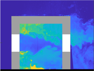
The differences in the flow field result in substantial disparities in scalar transport among the three configurations, as evident in both the instantaneous ( $C/C_S$, shown in natural logarithmic scale) concentration maps illustrated in figure 6, and the time-averaged concentration ( $\bar {C}/C_S$) and variance ( $\overline {{c^{\prime }}^2}/C^2_S$) in figure 7(a,b); here, the instantaneous concentration fluctuation ( $c^{\prime }$) is defined as, $c^{\prime }=C-\bar {C}$. Presently, the time-averaged concentration ( $\bar {C}/C_S$) is determined by performing an averaging over approximately 1000 instantaneous ( $C/C_S$) concentrations. In the representation in figures 6 and 7, and throughout the manuscript, the scalar concentration ( $C$) is normalized by the source strength ( $C_S$), following the approach outlined in previous studies (Reference Lim, Hertwig, Grylls, Gough, Van Reeuwijk, Grimmond and VanderwelLim et al. 2022; Reference Lim and VanderwelLim & Vanderwel 2023). Also to be noted is that these (processed) images were acquired after the flow through the cube and the concentration within the cube had reached a statistically steady state, in a mean sense. The side-view visualization of the instantaneous scalar fields ( $C/C_S$) in figure 6 shows the highly dynamic nature of the scalar fields across different time instances, revealing substantial variations in scalar concentration, spatio-temporal distribution within the cube and differences across three configurations. The differences in scalar transport across the three configurations are discussed below.
Instantaneous scalar fields ( $C$) normalized by the source concentration ( $C_S$), shown at $Re$ of 20 000, for three window configurations: (a) centre, (b) up-down and (c) down-up. These instantaneous scalar fields are shown at an interval of 0.2 $s$. Flow is from left to right.

Time-averaged (a) concentration ( $\bar {C}/C_S$, in natural log scale), and (b) concentration variance ( $\overline {c^{\prime }c^{\prime }}/C^2_S$, in natural log scale) in the centre plane, shown at $Re$ of 20 000, for three building configurations. The area average of the time-averaged concentration ( $\overline {C_a}$) is given in table 1.

3.1.1 Centre
We now begin with the ‘centre’ configuration in figure 5(a(i)), where we observe a jet traversing through the cube and two re-circulation regions ( $R_{up}$, $R_{low}$) adjacent to the top and bottom walls, as demarcated by white (dashed) closed lines. In this configuration, the temporal evolution of the flow revealed the vertical oscillation or flapping of the jet. In addition to the mean flow, the in-plane turbulent kinetic energy (( $\overline {u^{\prime }u^{\prime }}+\overline {v^{\prime }v^{\prime }})/U^2_{Ref}$) in figure 5(b(i)) shows dominant behaviour inside the cube at the interface of the jet and the reverse flow regions. Such dynamic behaviour of the indoor flow carries potential implications for scalar transport within the cube, as we will discuss now.
In the ‘centre’ configuration (figure 6a), there is a notable accumulation of scalar in the re-circulation regions near the top and bottom walls of the cube, with relatively higher scalar strength near the bottom wall, as further clearly visible from the time-averaged scalar concentration ( $\bar {C}/C_S$) in figure 7(a(i)). In this case, the side-view time-series scalar maps reveal that the scalar introduced near the source is transported towards the upstream wall (along ( $-$)ve $x$) through the reverse flow within the lower re-circulation region ( $R_{low}$, figure 5a(i)). Subsequently, some of the transported scalar is carried upwards (towards ( $+$)ve $y$) and then downstream (towards ( $+$)ve $x$) and accumulates within $R_{low}$, and the rest of the scalar is transported into the jet. While the scalar trapped in the jet convects downstream with the jet, a portion of the scalar parcel is observed to be transported into both the upper ( $R_{up}$) and lower ( $R_{low}$) re-circulation regions. This phenomenon may be attributed to the vertically oscillating nature of the jet and the development of instability at the interface between the jet and $R_{up}$ and $R_{low}$, as also evident from the formation of interfacial structures in figure 6(a(ii)). Following these processes, a fraction of the scalar (from the jet) is flushed out of the cube, while the remainder accumulates in the upper and lower re-circulation regions. It may be noted that this cube with centred windows would be expected to have re-circulation within the plane normal to the jet axis, in addition to the ones in the streamwise planes, which could also play an important role in governing the scalar distribution between the regions below and above the jet axis. It can be noted that our focus throughout the manuscript is primarily on the mean characteristics of the scalar rather than transient behaviours, and hence, the time-varying statistics will not be discussed in detail.
3.1.2 Up-down
In the ‘up-down’ configuration in figure 5(a(ii)), we observe a jet positioned near the top wall, advancing towards the leeward wall and subsequently redirecting downward toward the window downstream. Notably, we identify a reverse flow region closer to the bottom wall, albeit relatively weaker when compared with the ‘centre’ configuration. On the other hand, ( $\overline {u^{\prime }u^{\prime }}+\overline {v^{\prime }v^{\prime }})/U^2_{Ref}$ exhibits prominence only within the jet inside the cube.
In the time-series images of the scalar fields, we observe an initial transport of the scalar from the source toward the upstream (in ( $-$)ve $x$), as also evident from the mean and the instantaneous scalar maps in figures 7(a(ii)) and 6(b(ii)), respectively. This transport is facilitated by the reverse flow within $R_{low}$, similar to the ‘centre’ configuration. Subsequently, the transported scalar undergoes redirection vertically (( $+$)ve $y$) nearly in the midway ( $x/H\approx -0.25$), and then towards the streamwise direction (along ( $+$)ve $x$) and finally is transported downstream towards the exit. During this process, there is minimal scalar transport into the jet passing near the top wall, thus not allowing any notable accumulation of the scalar near the top wall. As seen in the instantaneous maps, the scalar, which is occasionally seen penetrating the jet, is further carried by the jet and eventually flushed out of the cube. This configuration exhibits scalar accumulation solely in the lower half of the cube, with almost no scalar in the upper region, as clearly seen in the time-averaged concentration ( $\bar {C}/C_S$) in figure 7(a(ii)).
3.1.3 Down-up
Moving on to the ‘down-up’ configuration in figure 5(a(iii)), we observe a re-circulation region near the top wall spanning a relatively larger area in the upper half of the cube. Simultaneously, a jet is positioned near the bottom wall, passing in very close proximity to the scalar source. This jet eventually redirects vertically and subsequently towards the window downstream. On the other hand, ( $\overline {u^{\prime }u^{\prime }}+\overline {v^{\prime }v^{\prime }})/U^2_{Ref}$ exhibits prominence only within the jet, similar to the ‘up-down’ configuration. In the ‘down-up’ configuration, as illustrated in figure 7(a(iii)), we observe the initial transport of the scalar from the source toward the downstream wall. While the scalar from here undergoes redirection in the wall-normal direction (along ( $+$)ve $y$), a portion of it gets trapped in the reverse flow region in the upper half of the cube, while the rest of it is flushed out through the window downstream.
Table showing the time average of the ‘area-averaged concentration’ ( $\bar {C}_{a}/C_S$) and the standard deviation of the ‘instantaneous area-averaged concentration’ ( ${\sigma }_{C_{a}}/\overline {C_{a}}$), obtained over stage ‘III’ for different window configurations and Reynolds numbers.

3.1.4 Comparison
Among the three configurations studied, the ‘centre’ configuration exhibits the most accumulation of scalar within the cube, as evident from the comparison of time-averaged scalar maps across figure 7(a(i–iii)), and also in the time average of the area-averaged scalar (  $\overline {C_a}/C_S$) shown in table 1. This is followed by ‘up-down’ being the intermediate one, and the last configuration, ‘down-up’, exhibits the least scalar concentration build-up within the cube among all three configurations, as evident from both $\bar {C}/C_S$ in figure 7 and $\overline {C_a}/C_S$ in table 1. Similar to the mean concentration, the concentration variance ( $\overline {c^{\prime }c^{\prime }}/C^2_S$) shown in figure 7(b) closely resembles the mean concentration ( $\bar {C}/C_S$) in terms of its preferential distribution and variations across different configurations. The standard deviation of the ‘area-averaged instantaneous concentration’ ( ${\sigma }_{C_{a}}$) is an indicator of the unsteadiness of the flow. The standard error associated with $\overline {C_a}$ and ${\sigma }_{C_{a}}$, as shown in table 1, is determined using the bootstrap method (Reference Efron and TibshiraniEfron & Tibshirani 1986; Reference Davison and HinkleyDavison & Hinkley 1997). These errors in the mean and standard deviation are found to be less than $3\,\%$ and $5\,\%$, respectively, thus establishing confidence in the measurements.
The current concentration maps for various configurations show similarities with those observed by Reference Tominaga and BlockenTominaga & Blocken (2016) regarding the spatial distribution of the scalar. In both our work and theirs, the ‘down-up’ configuration exhibits the lowest scalar concentration in terms of the steady-state concentration ( $\overline {C_a}/C_S$) magnitude. This can be attributed to the stronger flow velocity near the source and a shorter path for the scalar to reach the downstream window compared with the other configurations, as evident from the velocity maps in figure 5(a). This suggests that the source's position relative to the window(s) is a critical factor. Another noteworthy aspect is that the order for the other two configurations (‘down-up’ < ‘up-down’ < ‘centre’) seems slightly different from that reported by Reference Tominaga and BlockenTominaga & Blocken (2016) (‘down-up’ < ‘centre’ < ‘up-down’). The reason for the difference can be explained again by considering the length of the streamline between the source and the exit window. The re-circulation regions in the present configurations are more three-dimensional in nature and hence would be expected to have longer (out-of-plane) path lines for the scalar to reach the downstream window, while in Reference Tominaga and BlockenTominaga & Blocken (2016), due to the higher window aspect ratio, the re-circulations would be more two-dimensional and have a shorter scalar path.
To summarize, we find that both the concentration and its variance vary dramatically across different window configurations in terms of their preferential accumulation, peak concentration and transport mechanisms. The statistically equilibrated concentration within the cube was notably highest for the ‘centre’ configuration, followed by the ‘up-down’ and ‘down-up’ configurations. Concerning scalar distribution, the ‘centre’ configuration has scalar accumulation near the top and bottom walls in the re-circulation regions, with the peak concentration being near the source and the near-ground corner areas upstream. Also seen is the relatively non-uniform scalar concentration in the lower part of the cube. In comparison, the ‘up-down’ configuration has a relatively uniform scalar buildup in the lower half of the cube, except for closer to the source. In contrast, the ‘down-up’ configuration has a nearly uniform scalar buildup in the upper half of the cube, with peak concentration near the source and the near-ground inside corner downstream of the cube. These broad differences are reflected again in figure 8, showing the wall-normal ( $y/H$) profiles of the velocity and concentration at the source ( $x/H=0$), upstream ( $x/H=-0.25$) and downstream ( $x/H=0.25$) to the source, and also outside the cube, at $x/H=0.75$, clearly indicating the substantial influence of the window positioning on scalar transport. Another aspect to note from the velocity profiles in figure 8 would be that the inlet jet flow speed at the window level is the highest for ‘centre’, followed by the ‘up-down’ and ‘down-up’ configurations. The ‘up-down’ configuration, despite facing the highest oncoming flow speed upstream at the window level, does not have the highest inflow jet speed since it is not just the height of the window from ground level that matters but also the relative placement of the window downstream which would affect it.
Wall-normal ( $y/H$) profiles of: (a–c(i)) mean streamwise velocity ( $\bar {U}/U_{Ref}$); (a–c(ii)) mean concentration ( $\bar {C}/C_S$, in log scale); and (a–c(iii)) concentration variance ( $\overline {c^{\prime }c^{\prime }}/C^2_S$, in log scale), at streamwise locations of $x/H=-0.25, 0, 0.25$, all within the cube, and at $x/H=0.75$, outside the cube, shown at $Re=20\ 000$, for the centre, up-down and down-up configurations. (a) Centre, (b) up-down and (c) down-up.

Now, coming to the scalar concentration, despite the ‘centre’ configuration having the highest window-level jet inflow speed, it has the most scalar build-up, while ‘down-up’ with the lowest inflow jet speed has the least scalar concentration. This indicates that the position of the source relative to the window is more critical in governing the indoor scalar build-up in such cross-ventilating flows, which has also been indicated recently by Reference Lim, Foat, Parker and VanderwelLim et al. (2024).
3.2 Advective and turbulent scalar transport
To better understand the scalar distribution within the model, we discuss further the scalar transport in the bulk flow, in terms of the advective flux, and also the turbulent flux representing the scalar transport by the variance in the velocity and scalar. We present in figure 9 the advective ( $\bar {C} \bar {U}/C_SU_{Ref}$, $\bar {C} \bar {V}/C_SU_{Ref}$) and the turbulent ( $\overline {c^{\prime }u^{\prime }}/C_SU_{Ref}$, $\overline {c^{\prime }v^{\prime }}/C_SU_{Ref}$) scalar fluxes, encompassing both streamwise and wall-normal components; here, $\bar {V}$ represents the time-averaged wall-normal velocity. Focusing on the ‘centre’ configuration in figure 9(a(i),b(i)), we observe in close proximity to the source a ( $-$)ve $\bar {C} \bar {U}/C_SU_{Ref}$, transporting the injected scalar towards the upstream wall. This results in a higher localized concentration around the cube's left corner, as seen previously in figure 7(a(i)). Simultaneously, from the corner area, a ( $+$)ve $\bar {C} \bar {V}/C_SU_{Ref}$ transports the scalar upward towards the jet. This jet shows a relatively stronger ( $+$)ve $\bar {C} \bar {U}/C_SU_{Ref}$ facilitating the transport of scalar outward from the cube. Unlike the advective fluxes, the turbulent scalar fluxes in figure 9(c(i),d(i)) seem strongest around the interface of the jet and re-circulation flow regions. The streamwise component ( $\overline {c^{\prime }u^{\prime }}/C_SU_{Ref}$) is found to be ( $-$)ve, indicating its role in scalar transport opposite to the streamwise direction. In contrast, the ( $+$)ve and ( $-$)ve wall-normal fluxes ( $\overline {c^{\prime }v^{\prime }}/C_SU_{Ref}$) in $R_{low}$ and $R_{up}$, respectively, indicate the transport of scalar from the re-circulation regions into the jet. It may be noted that the convective flux is approximately one order of magnitude stronger than the turbulent counterpart in all window configurations.
(a) Streamwise advective flux ( $\bar {C} \bar {U}/C_SU_{Ref}$), (b) wall-normal advective flux ( $\bar {C} \bar {V}/C_SU_{Ref}$), (c) streamwise turbulent flux ( $\overline {c^{\prime }u^{\prime }}/C_SU_{Ref}$) and (d) wall-normal turbulent flux ( $\overline {c^{\prime }v^{\prime }}/C_SU_{Ref}$), at $Re$ of 20 000, shown for three building configurations.

Moving on to the ‘up-down’ configuration in figure 9(a(ii),b(ii)), a ( $+$)ve $\bar {C} \bar {V}/C_SU_{Ref}$ is identified, conveying scalar from the lower re-circulation region into the jet and directed towards the exit window by a ( $+$)ve $\bar {C} \bar {U}/C_SU_{Ref}$ along the jet. The streamwise turbulent flux, $\overline {c^{\prime }u^{\prime }}/C_SU_{Ref}$ (in figure 9c(ii)) appears prominent at the interface of the jet and reverse flow region. However, this being ( $-$)ve indicates its role in transporting the scalar opposite to the streamwise direction, enhancing scalar mixing in the room. In the ‘down-up’ configuration in figure 9(a(iii),b(iii)), a ( $+$)ve $\bar {C} \bar {U}/C_SU_{Ref}$ facilitates scalar transport from the source towards the downstream wall, followed by a ( $+$)ve $\bar {C} \bar {V}/C_SU_{Ref}$ that carries the scalar towards the top wall and is subsequently flushed out by the ( $+$)ve $\bar {C} \bar {U}/C_SU_{Ref}$. Now, looking at these transport mechanisms and the respective scalar accumulations in these configurations (in figure 7a), it would be notable that, despite the ‘down-up’ configuration exhibiting relatively weaker fluxes, the scalar buildup is minimal, as was noted in figure 7(a(iii),b(iii)). The broad observations discussed in this section suggest that the advective flux mostly influences the ventilation rate while the turbulent scalar fluxes contribute to the mixedness.
3.3 Time scales
Thus far, we have discussed the dispersion characteristics during the period of statistically steady concentration within the cube, stage ‘III’, attained after scalar injection is initiated. This section discusses the time scales associated with the scalar buildup within the cube and flushing out of the cube, in stages ‘II’ and ‘IV’, respectively, and also the concentration obtained from the area averaging ( $C_a$). We begin with the noticeable variations observed across these configurations in both the scalar build-up and flushing rates. This is evident in figure 10(a–c) and also from the scalings for $C_a$ with dimensionless time ( $t^{\ast } = tU_{Ref}/H$) presented in table 2. It may be noted here that, to obtain these scalings, the stage ‘II’ is defined based on the time span from time $t_{01}$ until $C_a$ approaches the value close to the time-averaged ‘area average of the concentration’ ( $\overline {C_a}$) obtained over stage ‘III’, which would be the statistically steady concentration (from table 1). On the other hand, stage ‘IV’ spans from time $t_{02}$ until $C_a$ reaches the background concentration, closer to zero, as was illustrated in figure 4(a). Also to be noted is that the exponents for the scalings in table 2 are found to be relatively insensitive to the upper cutoff limits of $C_a$ defining the spans for the stages ‘II’ and ‘IV’.
The area-averaged scalar concentration ( $C_{a}/C_S$) within the cube, from the experiments at $Re$ of 20 000, plotted against time ( $tU_{Ref}/H$), along with the fits using (2.8) (——–, black) and (3.1) ( $\hspace{0.01em}{\rule[0.5ex]{0.5em}{1pt}}\hspace{0.1em}{\rule[0.5ex]{0.5em}{1pt}}\hspace{0.1em}{\rule[0.5ex]{0.5em}{1pt}}\hspace{0.01em}$, red), from the revised ‘box model’. (a) Centre, (b) up-down and (c) down-up.

Table showing the scalings for  $C_{a}/C_S$ with $t^{\ast }$ in the scalar build-up and flushing periods, the mean values of the exit-to-indoor concentration ( $\alpha$) and its standard deviation ( ${\sigma }_{\alpha }/\alpha$) and the additional factors in the revised box model in (3.1), all shown for $Re$ of 20 000. In the topmost row, the respective stages, as in (3.1), have also been indicated.

Moving forward, we discuss with figure 10 the area-averaged concentration ( $C_a$), plotted against time, over all the stages ‘I’ to ‘V’. Notably, in the stage ‘III’, the concentration is highest for the centre building, followed by the ‘up-down’ and ‘down-up’ configurations, as was evident previously with figure 7. Large fluctuations in $C_a$ during stage ‘III’ are also observed in figure 10, as also noted by its standard deviation ( ${\sigma }_{C_a}$, over stage ‘III’) in table 1, which would be attributable to the dynamic nature of the flow within the box. The concentration ( $C_a$) plotted with time from experiments is further compared with the one calculated from the revised box model using (2.8) (——– (black), figure 10), from § 2.3. As seen in figure 10, the revised model effectively matches the concentration profile from the experiments, except for the scalar build-up and flushing stages for the ‘up-down’ and ‘down-up’ configurations, in figure 10(b,c). To address this, two additional factors, $\gamma _{1}$ and $\gamma _{2}$, are introduced into (2.8) for stages ‘II’ and ‘IV’, respectively. The revised version of (2.8), as given below in (3.1), now reasonably aligns (– – – (red), figure 10) with the experimental data across all stages
 \begin{equation} C_{I-V} = \underbrace{C_n}_{I \& V} + \underbrace{\frac{1}{{\alpha}{\beta}}\frac{C_SQ_S}{A_oU_{o}} (1-{\rm e}^{-({{\gamma_{1}}{\alpha}U_{o}A_o}/{V_m}) (t-t_{01})})}_{II + III} + \underbrace{{C_{t_{02}}}\, {\rm e}^{-({{\gamma_{2}}{\alpha}U_{o}A_o}/{V_m}) (t-t_{02})}}_{IV}. \end{equation}
 One should note that these factors ( $\alpha$, $\beta$, $\gamma _1$, $\gamma _2$) may exhibit large variations across different building configurations, as indicated in table 2. To further emphasize the pivotal role of these introduced factors, we calculated the concentration from the non-revised box model, assuming the values for these factors set to unity ( $\alpha$, $\beta$, $\gamma _1$, $\gamma _2$=1) and $C_n$ set to be zero in (3.1). Notably, in the equilibrium stage ‘III’, from the non-revised model, the concentration is seen to be approximately one order of magnitude smaller than in experiments. The non-revised model also informs the scalar concentration in stage ‘III’ to follow the sequence of ‘down-up’ > ‘up-down’ > ‘centre’, contrary to the observed trends from experiments. These differences are expected due to several assumptions inherent in the model. For instance, the model assumes instantaneous and uniform mixing of the injected scalar occurring within the CV and also does not account for the changes in flow patterns within the cube resulting from the window repositioning. Accounting corrections for these, the modified version of the ‘box model’, as in (3.1), hence, would be a more sensible reflective of the pollutant concentration in practical scenarios.
3.3.1 Mixedness
Presently, scalar concentration measurements have only been performed in the vertical mid-plane passing through the centre of the windows and the source. However, since the jet and re-circulation regions governing the scalar transport and volumetric mixing would be three-dimensional due to the shorter aspect ratio of the openings, it is important to characterize the inhomogeneity of the scalar concentration in the out-of-plane direction, which we have performed once using the revised box model (mixedness,  $\beta$). Now, another way to obtain this mixedness would be by performing a mass balance on the scalar, assuming a two-dimensional pattern of scalar concentration and velocity at the exit window. From the measured velocity and concentration in the centre plane, we know the outflow velocity ( $U_o$) and the scalar concentration ( ${C_o}$) at the exit window. Now, assuming a two-dimensional out-of-plane pattern for $C_o$ and $U_o$, the total scalar mass exiting through the downstream window would be $A_oU_oC_o$. However, this calculated value is found not to be equal to the injected scalar mass at the source, $C_SQ_S$, indicating an out-of-plane inhomogeneity in the scalar concentration. We can characterize and quantify this inhomogeneity (similar to the revised box model) in terms of another mixedness factor, ${\beta }_o = C_SQ_S/(A_oU_oC_o)$. Now, in a truly two-dimensional flow, ${\beta }_o$ should be equal to 1, since the scalar concentration would be homogeneous along the out-of-plane directions. However, the calculated ${\beta }_o$ values are found to be approximately 0.048, 0.065 and 0.189 for the ‘centre’, ‘up-down’ and ‘down-up’ configurations, respectively. This implies a spanwise inhomogeneity in concentration, and the total volumetric scalar concentration estimated from the centre plane concentration measurements would be higher than the actual concentration by a factor of $1/{\beta }_o$. It may be noted that ${\beta }_o$ closely match with the mixedness from the revised box model ( $\beta$, in table 2), thus establishing confidence in the calculated out-of-plane scalar inhomogeneity. It is also worth noting that the mixedness is significantly higher for the ‘down-up’ configuration, implying a relatively well-mixed scalar concentration compared with the ‘centre’ and ‘up-down’ configurations.
3.3.2 Ventilation effectiveness
We have already observed that the ‘centre’ configuration exhibits the most accumulation of scalar within the cube, followed by the ‘up-down’ and ‘down-up’ configurations. Now, in addition to discussing the equilibrium concentration in stage ‘III’, it is also essential to compare the scalar building and flushing time scales across the three configurations, as obtained from stages ‘II’ and ‘IV’ in figure 10. The scalings of the area-averaged scalar concentration ( $C_{a}/C_S$) with time ( $t^{\ast }$) in these stages are presented in table 2. One can observe from the scalings that the scalar buildup is quickest for the ‘up-down’ configuration and considerably slower for the ‘down-up’ and ‘centre’ configurations, with minimal differences between the latter two. On the other hand, flushing is fastest for the ‘down-up’ configuration, followed by the “up-down and ‘centre’ configurations. It may also be noted that these orders for different windows in stages ‘II’ and ‘IV’ do not follow the sequence from stage ‘III’ for the steady-state concentration. Overall, the results show that the ‘down-up’ configuration leads to relatively slower indoor scalar buildup, minimal steady-state concentration and faster scalar flushing rate. These would be attributed to the higher flow velocity near the source and a shorter path for the scalar to reach the downstream window in ‘down-up’ compared with the other configurations, thus making it the favourable design among the three window configurations to ensure the least pollutant concentration in an indoor environment.
3.4 Effects of Reynolds number
We have seen at a fixed  $Re$ of 20 000 window positions resulting in substantial differences in flow patterns, leading to dramatic differences in the scalar concentration. We investigated further two more $Re$ ( $\approx$35 000, 50 000), looking into the flow patterns and concentration fields. We find the flow characteristics to be nearly independent of the incoming flow $Re$, for example, shown in figure 11(a(i),b(i)) is $\bar {U}/U_{Ref}$ for the ‘centre’ configuration at $Re$ values of 20 000 and 50 000. This results in nearly identical scalar distribution within the cube, as seen in figure 11(a(ii),b(ii)). In addition, we find at each of these larger $Re$ cases of 35 000 and 50 000, the mean (over time) of the area-averaged concentration ( $\overline {C_a}/C_S$) to be the highest for the ‘centre’, followed by the ‘up-down’ and the ‘down-up’ configurations, similar to the cases seen for $Re$ of 20 000, as summarized in table 1. However, to be noted is that, for a fixed window configuration, although the scalar distribution is nearly identical for different $Re$, as seen in figure 11(a(ii),b(ii)), their magnitude is substantially lower at higher $Re$, which would be expected due to the smaller flow time scale (larger flow speed). Now, for a fair comparison of the changes in the concentration for a fixed building across different $Re$, the modified flow speed is accounted for in the scalar concentration following a more generalized non-dimensional form, as $\tilde {C}={\overline {C_a}U_{Ref}{H}^2/C_SQ_S}$, following previous studies on indoor and outdoor dispersion in urban environments (e.g. Reference RobinsRobins 1980; Reference SnyderSnyder 1981; Reference Daniela, Marco Túllio, Tiziano and BardoDaniela et al. 2012; Reference Xia, Niu and LiuXia, Niu & Liu 2014; Reference Tominaga and BlockenTominaga & Blocken 2016). Following this normalization, we find, for a fixed window configuration, the changes in $\tilde {C}$ across different $Re$ to be smaller than the large drop in $\overline {C_a}/C_S$ with increasing $Re$ (in table 1), for example, as seen in the area-averaged ‘time-averaged concentration’ ( $\tilde {C}$) for all the cases studied in table 3, and the time-averaged concentration maps in figure 11(a(iii),b(iii)) for $Re$ of 20 000 and 50 000. These broad observations indicate that the scalar transport in such cross-ventilating flow configurations would be nearly independent of the Reynolds number.
(i) Time-averaged streamwise velocity ( $\bar {U}/U_{Ref}$), and (ii,iii) time-averaged concentration following two different normalizations ( $\bar {C}/C_S$ and $\bar {C}U_{Ref}{H}^2/C_SQ_S$), at $Re$ of (a) 20 000 and (b) 50 000.

Table showing the area average of the ‘time-averaged concentration’ following a different normalization,  ${\overline {C_a}U_{Ref}{H}^2/C_SQ_S}$, obtained over stage ‘III’, for different window configurations and Reynolds numbers.

4. Conclusions and recommendations
In urban environments, cross-ventilation could play a critical role in dispersing indoor pollutants by promoting the exchange of indoor and outdoor air. To comprehend the transport of pollutants within such intricate scenarios, we experimentally investigated an idealization of these, namely, a flow through a hollow cube (approximately 40 : 1), with windows upstream and downstream and a passive scalar (fluorescent dye) source inside, immersed in a rough-wall turbulent (water) boundary layer. The primary focus was on the characterization of the scalar transport within the cube and towards the external environment through simultaneous measurements of the scalar and the flow, using PLIF and PIV, respectively. These measurements were conducted at different incoming flow Reynolds numbers ( $Re=20\ 000$, 35 000 and 50 000) for three distinct configurations: ‘centre’, ‘up-down’ and ‘down-up’, categorized based on the respective locations of the upstream and downstream windows.
Dramatic alterations in flow patterns within the cube were observed due to variations in window positioning, resulting in significant differences in scalar transport, concentration and distribution among different configurations. The (statistical) equilibrium concentration within the cube was notably highest for the ‘centre’ configuration, followed by the ‘up-down’ and ‘down-up’ configurations. Concerning scalar distribution, the ‘centre’ exhibited scalar accumulation near the top and bottom walls in re-circulation regions, with the peak concentration around the source and the upstream near-ground corner. Additionally, non-uniform scalar concentration was noticeable in the lower part of the cube. In comparison, ‘up-down’ showed a relatively uniform scalar buildup in the lower half of the cube, with peak concentration around the source. Conversely, ‘down-up’ showcased a nearly uniform scalar buildup in the upper half of the cube, with peak concentration near the source and the near-ground corner downstream. Furthermore, distinct variations were observed across three configurations in both scalar buildup and flushing rates. These overall flow characteristics, scalar transport modes, concentrations and distributions were nearly independent of the incoming flow Reynolds number under each configuration.
The analysis of scalar transport was extended by employing a simplified ‘box model’ that showed the concentration to be approximately one order of magnitude lower than observed in the experiments. This discrepancy from the model was due to assumptions such as perfect mixing of the scalar and not accounting for changes in flow patterns within the cube resulting from window repositioning. To align the model with the experiment, we introduced several factors, including mixedness, into the model and proposed a modified ‘box model’ that could reflect pollutant concentrations in practical scenarios with more accuracy, accounting for complexities such as non-perfect mixing and changes in flow patterns.
In connection with the present findings, several prospects for potential future investigation remain open.
(1) The present model with a single window can be further modified to more realistic building designs that typically incorporate multiple smaller windows.
(2) Future investigations can incorporate scalar injection from an elevated location mimicking pollutant source at breathing levels, which would be one step closer to the modelling of an infectious aerosol introduced into the building interior.
(3) The current results would help inform future water-tunnel and wind-tunnel studies, and CFD simulations, exploring other parameters, such as buoyancy and ventilation, in more complex geometries.
Overall, this study provides thorough insights into the influence of window placements on flow characteristics and scalar transport mechanisms, simultaneously, within indoor settings for an indoor–outdoor cross-ventilating scenario. The findings will contribute to improved comprehension and characterization of the dispersion of indoor pollutants, elucidating their preferential distributions, peak concentrations and durations of accumulation and flushing. Furthermore, insights from the modified box model will inform the existing models, facilitating better accuracy in their predictions of dispersion concentration in intricately structured urban environments.
Acknowledgement
S.B. thanks Y. Elashmawi, T. Rich and D. Clements for helping with the experiments.
Funding statement
The authors gratefully acknowledge funding by UK Research and Innovation (Project Reference: MR/S015566/1).
Declaration of interests
The authors declare no conflict of interest.
Author contributions
Subhajit Biswas: Investigation, Methodology, Data curation, Validation, Writing – original draft, review & editing. Christina Vanderwel: Conceptualization, Supervision, Writing – review & editing.
Data availability statement
Data are made available in the University of Southampton data repository at https://doi.org/10.5258/SOTON/D3169.
Ethical standards
The research meets all ethical guidelines, including adherence to the legal requirements of the study country.


 Open access