Nomenclature
- ${\mathcal{W}}$
-
wind (m/s)
-
$W$
-
waypoints
-
$A$
-
segments
-
$f$
-
flight
-
${R_E}$
-
Earth radius (m)
-
$l$
-
length of segment (m)
-
$V$
-
flight speed s (m/s)
-
${\mathcal{T}}$
-
studied time period
-
$T$
-
flight time ensemble
-
$\Delta T$
-
time from departure to the entry point of the target airspace
-
$r$
-
lateral trajectory
-
$G$
-
graph
-
${\mathcal{S}}$
-
four-dimensional sampling point
-
$\Delta d$
-
sampling distance (km)
-
${N_v}$
-
vertical sep a ration (ft)
-
${N_h}$
-
lateral separation (NM)
-
$D$
-
flight delay s (min)
-
$DT$
-
maximum time deviation (min)
-
${\mathcal{G}}$
-
Gini coefficient


List of symbols
-
$\lambda $
-
latitude
-
$\phi $
-
longitude
-
${\rm{\Delta }}$
-
grid resolution
-
$h$
-
altitude
-
${\theta _w}$
-
wind direction angle
-
${\theta _i}$
-
segment direction angle of
${a_i}$
-
${\sigma _f}$
-
departure time of flight
$f$
-
${\mu _{f,i}}\left( {{\sigma _f}} \right)$
-
expected flight times of
$f$
on segment
${a_i}$
under
${\sigma _f}$
-
${\delta _{f,i}}\left( {{\sigma _f}} \right)$
-
flight time deviation of
$f$
on segment
${a_i}$
under
${\sigma _f}$
-
${{\rm{\Phi }}_f}\left( {{\sigma _f}} \right)$
-
set of expected flight times on each segment under
${\sigma _f}$
-
${{\rm{\Omega }}_f}\left( {{\sigma _f}} \right)$
-
set of flight time deviations on each segment under
${\sigma _f}$
-
${{\rm{\varphi }}_f}\left( {{\sigma _f}} \right)$
-
total flight time expectation of
$f$
under
${\sigma _f}$
-
${{{\unicode{x03C8} }}_f}\left( {{\sigma _f}} \right)$
-
cumulative flight time deviation of
$f$
under
${\sigma _f}$
-
${{{\unicode{x03C8} }}_{f,0}}$
-
predefined allowed deviation threshold
-
${\bar{\mathrm{\Phi}}_{f,i}}$
-
expected flight time of segment
${a_i}$
over the entire planning horizon
$\left[ {0,\boldsymbol{\mathcal{T}}} \, \right]$


1.0 Introduction
The continuous growth of air traffic flow has led to a serious imbalance between airspace demand and capacity, reducing operational efficiency and increasing safety risks. In response, it is essential to modernise air traffic management (ATM) systems to enhance airspace capacity, improve safety and reduce operational costs. Major nations, such as the US [Reference Yim1] and Europe [Reference Sky and Undertaking2], are actively promoting ATM systems modernisation programmes to achieve these objectives.
Modern systems incorporate advanced technologies that reduce flight costs and increase airspace capacity. These technologies also improve operational safety by reducing the workload of air traffic controllers. Among these, trajectory planning is regarded as one of the core technologies. Trajectory planning can be classified as tactical or strategic based on the planning time horizon [Reference Courchelle, Soler, González-Arribas and Delahaye3]. Strategic trajectory planning (STP) addresses large-scale trajectory coupling from a global perspective, thereby reducing tactical interventions and improving overall airspace efficiency and safety. However, due to the longer lead time of STP, effective analysis of uncertainty – especially wind forecast uncertainty – is critical to ensuring the quality of large-scale trajectory plans. As a result, STP models that explicitly incorporate wind forecast uncertainty have become an increasingly important focus in recent ATM research.
STP typically consists of two main components: lateral trajectory planning (LTP) and conflict detection and resolution (CD&R). LTP aims to optimise individual flight paths to minimise operational costs, while CD&R addresses potential conflicts among large-scale trajectories from a system-wide perspective to ensure safety. Considering the influence of uncertainty, several approaches have been employed for LTP, including stochastic optimisation methods [Reference Franco Espín, Rivas Rivas and Valenzuela Romero4–Reference Geißer, Povéda, Trevizan, Bondouy, Teichteil-Königsbuch and Thiébaux6], control-theoretic models [Reference González-Arribas, Soler and Sanjurjo-Rivo7–Reference Kamo, Rosenow, Fricke and Soler10], and machine learning-based techniques [Reference Legrand, Puechmorel, Delahaye and Zhu11]. Among them, stochastic optimisation has been extensively studied. It is commonly formulated as a mixed-integer programming problem. Representative solution methods include classical path planning algorithms (e.g., Dijkstra and A* algorithms) [Reference Franco Espín, Rivas Rivas and Valenzuela Romero5, Reference Murrieta-Mendoza and Botez12, Reference Rosenow, Förster, Lindner and Fricke13], branch-and-bound algorithms [Reference Franco Espín, Rivas Rivas and Valenzuela Romero4] and heuristic algorithms [Reference Murrieta-Mendoza, Hamy and Botez14].
Under the influence of wind forecast uncertainty, identifying potential conflicts among large-scale trajectories is a key challenge in CD&R. Existing conflict detection methods can generally be divided into probabilistic and deterministic approaches. Probabilistic methods model aircraft spatiotemporal variables as random processes and compute conflict probabilities accordingly [Reference Jacquemart and Morio15–Reference Jilkov, Ledet and Li17]. In contrast, the deterministic approach expands the conflict protection zone according to spatiotemporal variables, and a conflict is identified when two protection zones overlap [Reference Courchelle, Soler, González-Arribas and Delahaye3]. The core of conflict detection lies in the accurate characterisation of trajectory uncertainty in both space and time. However, most existing methods analyse wind effects based on static snapshots. This approach may be insufficient because flights occur over long durations, and wind forecast uncertainty is highly time-variant. As a result, existing methods may fail to identify potential conflicts, reducing overall system efficiency. CD&R models typically resolve potential conflicts by adjusting parameters such as departure time (DT), flight level (FL), flight speed (FS) and lateral manoeuvring (LM) [Reference Dhief, Dougui, Delahaye and Hamdi18–Reference Dhief, Dougui, Delahaye and Hamdi23]. The objective is often to minimise trajectory deviations or the total number of conflicts [Reference Daniel, Oussedik and Stephane24]. Given the large-scale nature of the problem, CD&R is usually formulated as a combinatorial optimisation problem requiring substantial computational effort. Heuristic algorithms have been widely adopted in the literature due to their high computational efficiency. These methods are generally divided into individual-based and population-based algorithms. Examples of the former include simulated annealing (SA) [Reference Courchelle, Soler, González-Arribas and Delahaye3, Reference Mateos and Jiménez-Martín21, Reference Chaimatanan, Delahaye and Mongeau25], while the latter encompasses genetic algorithm (GA) [Reference Alam, Shafi, Abbass and Barlow26], non-dominated sorting genetic algorithm II (NSGA-II) [Reference Daniel, Oussedik and Stephane24], memetic algorithm (MA) [Reference Guan, Zhang, Han, Zhu, Lv and Su27], and multi-objective cooperative co-evolution algorithm (MOCCEA) [Reference Guan, Zhang, Lv, Chen and Michal16]. Table 1 provides a summary of recent studies on the computational performance of these algorithms.
The comparison between different CD&R algorithms in recent research

The studies reviewed above have rarely considered the influence of uncertainty in time-variant wind forecasts on STP. Given the long duration of flights and the dynamic nature of wind, trajectories optimised using static snapshot methods may still encounter unexpected conflicts during operation, which could compromise airspace safety. Fortunately, some related work has been undertaken. Although studies exist on planning under time-variant conditions like adverse weather [Reference Mothes32] and uncertain forecasts [Reference González-Arribas, Baneshi, Andrés, Soler, Jardines and García-Heras33], a key limitation remains. For instance, the approach in Ref. [Reference González-Arribas, Baneshi, Andrés, Soler, Jardines and García-Heras33], which discretises the planning horizon, does not account for conflicts among multiple aircraft. In reality, changes in departure times can alter the wind conditions encountered by the aircraft, potentially increasing operational costs and conflict risk. This highlights the lack of a comprehensive framework that jointly addresses LTP and CD&R considering time-variant wind forecast uncertainty. Solving large-scale CD&R models is computationally expensive, rendering traditional heuristics ineffective (see Table 1). While the MOCCEA framework addresses this via parallel computation, its sensitivity to the grouping strategy remains a challenge [Reference Guan, Zhang, Lv, Chen and Michal16]. Importantly, no studies have developed grouping strategies specifically to support parallel computation in this context.
To address these problems, this study models wind as a time-variant random variable and proposes a bilevel STP framework that integrates LTP and CD&R. The lower-level problem is formulated as a multi-objective optimisation model that aims to minimise conflicts and delays while ensuring fairness. Based on the departure times determined by the lower level, the upper-level model optimises the lateral trajectories within the permitted uncertainty range. The output of the bilevel model includes the optimal departure times, optimal lateral trajectories, estimated flight delays and the number of conflicts. To enhance computational efficiency, a dynamic equilibrium grouping (DEG) strategy is introduced to accelerate the performance of the MOCCEA by balancing computational loads across parallel threads. In addition, a time-variant A* (TVA*) algorithm based on a static expectation (SE) strategy is developed to search for the optimal lateral trajectory efficiently.
The structure of this paper is as follows: Section 2 presents the bilevel STP model considering time-variant uncertainty in wind forecasts; Section 3 introduces the proposed SE-based TVA * and the DEG-based MOCCEA; Section 4 applies the proposed methods to four scenarios to demonstrate their validity; and Section 5 concludes with the contributions of this paper and future directions.
2.0 Bilevel STP model
This section introduces the proposed bilevel strategic trajectory planning model, which explicitly accounts for time-variant wind forecast uncertainty. In simple terms, the bilevel model represents a two-layer decision-making framework. The upper-level determines the lateral trajectories of flights, aiming to minimise overall flight time within the acceptable range of uncertainty. The lower-level then adjusts the departure times to mitigate potential conflicts and balance fairness among flights. By integrating these two layers, the framework captures the coupling between trajectory optimisation and conflict resolution.
The remainder of this section is organised as follows. Section 2.1 describes the temporal characteristics of wind forecast uncertainty. Section 2.2 formulates the upper-level LTP model. Section 2.3 then presents the lower-level CD&R model.
2.1 Time-variant wind forecast uncertainty
Although wind is deterministic, forecast uncertainty is a time-variant random variable, particularly over strategic planning horizons. In most existing studies, wind forecast uncertainty is characterised using the ensemble prediction system (EPS). In this study, forecast data are obtained from the European Centre for Medium-Range Weather Forecasts (ECMWF), which provides forecast data at regular intervals with a temporal resolution of ${t_v}$
, generating a set of forecast data for each interval. Each set is valid within the time window ((
${t_v}$
, generating a set of forecast data for each interval. Each set is valid within the time window (( $n - 1$
)
$n - 1$
) ${t_v}$
,
${t_v}$
, $n{t_v}$
), where
$n{t_v}$
), where $n \in {N^ + }$
. We define the moment the wind field changes as a time-variant moment (TVM). Accordingly, the wind field
$n \in {N^ + }$
. We define the moment the wind field changes as a time-variant moment (TVM). Accordingly, the wind field $\overrightarrow {\boldsymbol{\mathcal{W}}\left( t \right)} $
is modelled as a piecewise function with discontinuities (see Fig. 1(a)) at time points
$\overrightarrow {\boldsymbol{\mathcal{W}}\left( t \right)} $
is modelled as a piecewise function with discontinuities (see Fig. 1(a)) at time points $\left\{ {{t_v},2{t_v},3{t_v}, \cdots } \right\}$
over the time domain
$\left\{ {{t_v},2{t_v},3{t_v}, \cdots } \right\}$
over the time domain $\left[ {0,\boldsymbol{\mathcal{T}}} \right]$
.
$\left[ {0,\boldsymbol{\mathcal{T}}} \right]$
.
Illustration of time-variant wind and angle definitions: (a) time-variant wind; (b) wind direction angle ${\theta _w}$
; (c) segment bearing angle
${\theta _w}$
; (c) segment bearing angle ${\theta _i}$
.
${\theta _i}$
.

This study addresses the STP problem within a free-route airspace (FRA), which represents a key direction in the future development of the ATM system. As FRA allows aircraft to plan flexible trajectories without relying on predefined airways, it becomes essential to discretise the airspace to model route choices effectively. The airspace, defined by the latitude range [ ${\lambda _{{\rm{min}}}}$
,
${\lambda _{{\rm{min}}}}$
, ${\lambda _{ax}}$
] and latitude range [
${\lambda _{ax}}$
] and latitude range [ ${\phi _{{\rm{min}}}}$
,
${\phi _{{\rm{min}}}}$
, ${\phi _{{\rm{max}}}}$
], is discretised into an
${\phi _{{\rm{max}}}}$
], is discretised into an $N \times M$
grid with a resolution of
$N \times M$
grid with a resolution of ${\rm{\Delta }}$
. The resulting grid nodes constitute the waypoint set
${\rm{\Delta }}$
. The resulting grid nodes constitute the waypoint set $W$
, while the connections between adjacent waypoints form the segment set
$W$
, while the connections between adjacent waypoints form the segment set $A$
[Reference Franco Espín, Rivas Rivas and Valenzuela Romero5]. The time-variant wind forecast data is mapped onto the discretised airspace grid. Accordingly, the wind at each waypoint is represented as a vector
$A$
[Reference Franco Espín, Rivas Rivas and Valenzuela Romero5]. The time-variant wind forecast data is mapped onto the discretised airspace grid. Accordingly, the wind at each waypoint is represented as a vector $\overrightarrow {\boldsymbol{\mathcal{W}}\left( t \right)} = \left( {{\boldsymbol{\mathcal{W}}_{EW}}\left( t \right),\;{\boldsymbol{\mathcal{W}}_{NS}}\left( t \right)} \right)$
, where
$\overrightarrow {\boldsymbol{\mathcal{W}}\left( t \right)} = \left( {{\boldsymbol{\mathcal{W}}_{EW}}\left( t \right),\;{\boldsymbol{\mathcal{W}}_{NS}}\left( t \right)} \right)$
, where ${\boldsymbol{\mathcal{W}}_{EW}}\left( t \right)$
and
${\boldsymbol{\mathcal{W}}_{EW}}\left( t \right)$
and ${\boldsymbol{\mathcal{W}}_{NS}}\left( t \right)$
denote the east–west and north–south wind components, respectively. In addition, each waypoint is associated with the following attributes: latitude (
${\boldsymbol{\mathcal{W}}_{NS}}\left( t \right)$
denote the east–west and north–south wind components, respectively. In addition, each waypoint is associated with the following attributes: latitude ( $\lambda $
), longitude (
$\lambda $
), longitude ( $\phi $
), altitude (
$\phi $
), altitude ( $h$
) and the wind vector
$h$
) and the wind vector $\overrightarrow {\boldsymbol{\mathcal{W}}\left( t \right)} $
. Based on this, the wind direction angle (
$\overrightarrow {\boldsymbol{\mathcal{W}}\left( t \right)} $
. Based on this, the wind direction angle ( ${\theta _w}\left( t \right)$
, see Fig. 1(b)) and wind magnitude (
${\theta _w}\left( t \right)$
, see Fig. 1(b)) and wind magnitude ( $||\overrightarrow {\boldsymbol{\mathcal{W}}\left( t \right)}|| $
) at each waypoint are computed.
$||\overrightarrow {\boldsymbol{\mathcal{W}}\left( t \right)}|| $
) at each waypoint are computed.
 \begin{align} {\theta _w}\left( t \right) = {\tan ^{ - 1}}\left\{ {\frac{{{\boldsymbol{\mathcal{W}}_{EW}}\left( t \right)}}{{{\boldsymbol{\mathcal{W}}_{NS}}\left( t \right)}}} \right\},\,||\overrightarrow {\boldsymbol{\mathcal{W}}\left( t \right)}|| = \sqrt {W_{EW}^2\left( t \right) + W_{NS}^2\!\left( t \right)} \end{align}
2.2 Upper-level model: LTP
2.2.1 Segment flight time prediction model
Given that the cruise phase constitutes most of the flight trajectory, focusing exclusively on optimising the cruise segment is reasonable. Assuming that the aircraft maintains a constant cruising altitude, let the coordinates of the start and end waypoints of segment ${a_i}$
are
${a_i}$
are $\left( {{\lambda _i},{\phi _i}} \right)$
and
$\left( {{\lambda _i},{\phi _i}} \right)$
and $\left( {{\lambda _{i + 1}},{\phi _{i + 1}}} \right)$
, respectively. In this study, the distance and bearing between two waypoints are computed using the rhumb-line (loxodrome) formulation, which assumes a constant bearing between consecutive waypoints. The bearing angle
$\left( {{\lambda _{i + 1}},{\phi _{i + 1}}} \right)$
, respectively. In this study, the distance and bearing between two waypoints are computed using the rhumb-line (loxodrome) formulation, which assumes a constant bearing between consecutive waypoints. The bearing angle ${\theta _i}$
and length
${\theta _i}$
and length ${l_i}$
of segment
${l_i}$
of segment ${a_i}$
(see Fig. 1(c)) are defined as follows:
${a_i}$
(see Fig. 1(c)) are defined as follows:
 \begin{align} \tan {\theta _i} = \frac{{{\phi _i} - {\phi _{i + 1}}}} {{\ln \left[ {\dfrac{{\tan \left( {\dfrac{\pi }{4} - \dfrac{{{\lambda _i}}}{2}} \right)}}{{\tan \left( {\dfrac{\pi }{4} - \dfrac{{{\lambda _{i + 1}}}}{2}} \right)}}} \right]}} \end{align}
 \begin{align}{l_i} = \left\{ {\begin{array}{*{20}{c}}{\dfrac{{\left( {{R_E} + h} \right)\left( {{\lambda _{i + 1}} - {\lambda _i}} \right)}}{{\cos {\theta _i}}},\,} {}{{\lambda _{i + 1}} \ne {\lambda _i}}\\[3pt]{\left( {{R_E} + h} \right)\cos {\lambda _i}\left| {{\phi _{i + 1}} - {\phi _i}} \right|,\,} {}{{\lambda _{i + 1}} = {\lambda _i}}\end{array}} \right. \\[2 pt] \nonumber \end{align}
The wind vector along the segment ${a_i}$
can be decomposed into a parallel wind component (
${a_i}$
can be decomposed into a parallel wind component ( ${\boldsymbol{\mathcal{W}}_{p,i}}\left( t \right)$
) and a crosswind component (
${\boldsymbol{\mathcal{W}}_{p,i}}\left( t \right)$
) and a crosswind component ( ${\boldsymbol{\mathcal{W}}_{c,i}}\left( t \right)$
). The crosswind is converted into an equivalent headwind to account for its impact on the effective ground speed. Accordingly, the ground speed (
${\boldsymbol{\mathcal{W}}_{c,i}}\left( t \right)$
). The crosswind is converted into an equivalent headwind to account for its impact on the effective ground speed. Accordingly, the ground speed ( ${V_{f,g,i}}\left( t \right)$
) and the corresponding flight time (
${V_{f,g,i}}\left( t \right)$
) and the corresponding flight time ( ${t_{f,i}}$
) of aircraft
${t_{f,i}}$
) of aircraft $f$
are calculated as follows:
$f$
are calculated as follows:
 \begin{align}{V_{f,g,i}}( t ) = \sqrt {V_{f,T}^2 - W_{c,i}^2\left( t \right)} + {\boldsymbol{\mathcal{W}}_{p,i}}\left( t \right) \\[-28pt] \nonumber \end{align}
 \begin{align}\frac{{d{l_i}}}{{d{t_{f,i}}\left( t \right)}} = {V_{f,g,i}}\left( t \right) \\[5pt] \nonumber \end{align}
where, ${V_{f,T}}$
is the true airspeed. According to Equation (5), for each time instant
${V_{f,T}}$
is the true airspeed. According to Equation (5), for each time instant $t \in \left[ {0,\boldsymbol{\mathcal{T}}} \right]$
, and for each ensemble member
$t \in \left[ {0,\boldsymbol{\mathcal{T}}} \right]$
, and for each ensemble member $\;k$
in the EPS, the corresponding flight time on segment
$\;k$
in the EPS, the corresponding flight time on segment ${a_i}$
can be represented as
${a_i}$
can be represented as $t_{f,i}^k\left( t \right)$
. Consequently, the flight time ensemble is defined as:
$t_{f,i}^k\left( t \right)$
. Consequently, the flight time ensemble is defined as: ${T_{f,i}}\left( t \right) = \left( {t_{f,i}^1\left( t \right),t_{f,i}^2\left( t \right), \cdots ,t_{f,i}^k\left( t \right), \cdots ,t_{f,i}^K\left( t \right)} \right)$
, where
${T_{f,i}}\left( t \right) = \left( {t_{f,i}^1\left( t \right),t_{f,i}^2\left( t \right), \cdots ,t_{f,i}^k\left( t \right), \cdots ,t_{f,i}^K\left( t \right)} \right)$
, where $K$
is the total number of ensemble members.
$K$
is the total number of ensemble members.
As previously noted, $\boldsymbol{\mathcal{W}}\left( t \right)$
is modelled as a piecewise function with discontinuities at time points
$\boldsymbol{\mathcal{W}}\left( t \right)$
is modelled as a piecewise function with discontinuities at time points $\left\{ {{t_v},2{t_v},3{t_v}, \cdots } \right\}$
. In this context, it becomes necessary to analyse the impact of such time-variant wind on consecutive flight segments. For example, suppose there are two consecutive segments
$\left\{ {{t_v},2{t_v},3{t_v}, \cdots } \right\}$
. In this context, it becomes necessary to analyse the impact of such time-variant wind on consecutive flight segments. For example, suppose there are two consecutive segments ${a_i}$
and
${a_i}$
and ${a_{i + 1}}$
, where aircraft
${a_{i + 1}}$
, where aircraft $f$
is subject to distinct wind fields
$f$
is subject to distinct wind fields $\boldsymbol{\mathcal{W}}1$
and
$\boldsymbol{\mathcal{W}}1$
and $\boldsymbol{\mathcal{W}}2$
, valid over the intervals
$\boldsymbol{\mathcal{W}}2$
, valid over the intervals $\left[ {0,{t_v}} \right]$
and
$\left[ {0,{t_v}} \right]$
and $\left( {{t_v},2{t_v}} \right)$
, respectively. Let the expected arrival times of aircraft
$\left( {{t_v},2{t_v}} \right)$
, respectively. Let the expected arrival times of aircraft $f$
at the origin and destination of segments
$f$
at the origin and destination of segments ${a_i}$
and
${a_i}$
and ${a_{i + 1}}$
be denoted by
${a_{i + 1}}$
be denoted by $t_{f,i}^o$
,
$t_{f,i}^o$
, $t_{f,i}^d$
,
$t_{f,i}^d$
, $t_{f,i + 1}^o$
and
$t_{f,i + 1}^o$
and $t_{f,i + 1}^d$
, respectively. Note that these segments are consecutive, so
$t_{f,i + 1}^d$
, respectively. Note that these segments are consecutive, so $t_{f,i}^d = t_{f,i + 1}^o$
. To determine the wind conditions experienced by aircraft
$t_{f,i}^d = t_{f,i + 1}^o$
. To determine the wind conditions experienced by aircraft $f$
on each segment, we use the expected arrival time at the origin of the segment as the basis. The following conditions are then established:
$f$
on each segment, we use the expected arrival time at the origin of the segment as the basis. The following conditions are then established:
Condition 1: if $t_{f,i}^o \lt {t_v}$
and
$t_{f,i}^o \lt {t_v}$
and $t_{f,i}^d \lt {t_v}$
, both segments
$t_{f,i}^d \lt {t_v}$
, both segments ${a_i}$
and
${a_i}$
and ${a_{i + 1}}$
are influenced by the wind field
${a_{i + 1}}$
are influenced by the wind field $\boldsymbol{\mathcal{W}}1$
. Accordingly,
$\boldsymbol{\mathcal{W}}1$
. Accordingly, ${T_{f,i}}\left( t \right) = T_{f,i}^1\left( t \right)$
and
${T_{f,i}}\left( t \right) = T_{f,i}^1\left( t \right)$
and ${T_{f,i + 1}}\left( t \right) = T_{f,i + 1}^1\left( t \right)$
.
${T_{f,i + 1}}\left( t \right) = T_{f,i + 1}^1\left( t \right)$
.
Condition 2: if $t_{f,i}^o \lt {t_v}$
and
$t_{f,i}^o \lt {t_v}$
and $t_{f,i}^d \ge {t_v}$
, then aircraft
$t_{f,i}^d \ge {t_v}$
, then aircraft $f$
experiences a wind transition at the end of segment
$f$
experiences a wind transition at the end of segment ${a_i}$
. In this case,
${a_i}$
. In this case, ${T_{f,i}}\left( t \right) = T_{f,i}^1\left( t \right)$
and
${T_{f,i}}\left( t \right) = T_{f,i}^1\left( t \right)$
and ${T_{f,i + 1}}\left( t \right) = T_{f,i + 1}^2\left( t \right)$
.
${T_{f,i + 1}}\left( t \right) = T_{f,i + 1}^2\left( t \right)$
.
This approximation is reasonable because: (1) the wind field is defined as a piecewise random function with independent intervals, so crossing a discontinuity naturally triggers a new wind realisation; (2) keeping each segment under a single wind condition avoids the need for further sub-division within a segment, thereby maintaining computational tractability; and (3) in practical trajectory planning, the temporal resolution of wind forecasts (e.g., at the hourly scale) is coarser than the duration of a single flight segment, so assuming segment-wise constancy of wind is a widely adopted and reasonable engineering simplification. A small-sample test (see Appendix A) shows that forcing segment splits at TVMs changes average flight time by at most ±0.3% and airspace-level conflicts by at most ±0.5%, confirming that the baseline treatment (no split) yields negligible bias for the chosen discretisation.
This study assumes that each segment’s flight time is independent. This assumption is widely used in trajectory planning under wind forecast uncertainty [Reference Franco Espín, Rivas Rivas and Valenzuela Romero4, Reference Franco Espín, Rivas Rivas and Valenzuela Romero5, Reference Kamo, Rosenow, Fricke and Soler10, Reference Legrand, Puechmorel, Delahaye and Zhu11] and remains reasonable in the time-variant setting considered here. Since $\overrightarrow {\boldsymbol{\mathcal{W}}\left( t \right)} $
is modelled as a piecewise random function with discrete transitions, the wind experienced on different segments can be considered conditionally independent, especially when aircraft traverse them at distinct TVMs. Moreover, this assumption allows the model to remain tractable while preserving sufficient fidelity for planning purposes.
$\overrightarrow {\boldsymbol{\mathcal{W}}\left( t \right)} $
is modelled as a piecewise random function with discrete transitions, the wind experienced on different segments can be considered conditionally independent, especially when aircraft traverse them at distinct TVMs. Moreover, this assumption allows the model to remain tractable while preserving sufficient fidelity for planning purposes.
To further verify this assumption, a small-sample statistical check was conducted using simulated trajectories. The Pearson correlation coefficients between consecutive segment flight times were calculated across 100 randomly selected flights. The average correlation coefficient was below 0.1, indicating a weak correlation between adjacent segments. This result confirms that the independence assumption between segment flight times is reasonable within the scope of this study. Therefore, the expected arrival times can be computed as follows:
 \begin{align}{\mu _{f,i}}\left( t \right) = \frac{1}{K}\mathop \sum \limits_{k = 1}^K t_{f,i}^k\left( t \right)\end{align}
 \begin{align}t_{f,i}^o = {\sigma _f} + \Delta T + \mathop \sum \limits_{\bar a \in \bar A} \mu _{f,i}^{\bar a}\left( t \right)\end{align}
 \begin{align}t_{f,i}^d = t_{f,i}^o + {\mu _{f,i}}\left( t \right)\end{align}
where ${\sigma _f}$
denotes the departure time of aircraft
${\sigma _f}$
denotes the departure time of aircraft $f$
,
$f$
, $\Delta T$
is the time from departure to the entry point of the target airspace, and
$\Delta T$
is the time from departure to the entry point of the target airspace, and $\bar A$
represents the set of segments traversed by aircraft
$\bar A$
represents the set of segments traversed by aircraft $f$
before segment
$f$
before segment ${a_i}$
. In this study,
${a_i}$
. In this study, $\Delta T$
is assumed to be a fixed constant for all flights, reflecting a uniform transition time before entering the planned airspace. Under this assumption, the
$\Delta T$
is assumed to be a fixed constant for all flights, reflecting a uniform transition time before entering the planned airspace. Under this assumption, the $t_{f,i}^o$
and
$t_{f,i}^o$
and $t_{f,i}^d$
are primarily influenced by the departure time
$t_{f,i}^d$
are primarily influenced by the departure time ${\sigma _f}$
and the cumulative expected flight times of the preceding segments. Therefore, in the following formulations, we use
${\sigma _f}$
and the cumulative expected flight times of the preceding segments. Therefore, in the following formulations, we use ${\sigma _f}$
as the representative variable to capture the temporal dynamics of each trajectory.
${\sigma _f}$
as the representative variable to capture the temporal dynamics of each trajectory.
2.2.2 Time-variant shortest path problem
A lateral trajectory ( ${r_f}$
) for aircraft
${r_f}$
) for aircraft $f$
can be represented as an ordered sequence of
$f$
can be represented as an ordered sequence of $n$
segments and their corresponding flight time ensembles, each of which depends on the departure time
$n$
segments and their corresponding flight time ensembles, each of which depends on the departure time ${\sigma _f}$
, i.e.,
${\sigma _f}$
, i.e.,
 \begin{align}{r_f} = \left\{ {\left( {{a_{f,1}},{T_{f,1}}\left( {{\sigma _f}} \right)} \right),\left( {{a_{f,2}},{T_{f,2}}\left( {{\sigma _f}} \right)} \right), \cdots ,\left( {{a_{f,i}},{T_{f,i}}\left( {{\sigma _f}} \right)} \right), \cdots ,\left( {{a_{f,n}},{T_{f,n}}\left( {{\sigma _f}} \right)} \right)} \right\},\\[2pt] \nonumber {a_{f,i}} \in A,\;{a_{f,i - 1}} \in A_{{a_{f,i}}}^ - ,\;\;{a_{f,i + 1}} \in A_{{a_{f,i}}}^ + ,\;{a_{f,i}} = \left( {{w_{f,i}},{w_{f,i + 1}}} \right),\;{w_{f,i}} \in W\end{align}
where, $A_{{a_{f,i}}}^ - $
denotes the set of segments entering waypoint
$A_{{a_{f,i}}}^ - $
denotes the set of segments entering waypoint ${w_{f,i}}$
, and
${w_{f,i}}$
, and $A_{{a_{f,i}}}^ + $
denotes the set of segments originating from waypoint
$A_{{a_{f,i}}}^ + $
denotes the set of segments originating from waypoint ${w_{f,i + 1}}$
. Accordingly, the set of all segments associated with
${w_{f,i + 1}}$
. Accordingly, the set of all segments associated with ${a_{f,i}}$
is defined as
${a_{f,i}}$
is defined as ${A_{{a_{f,i}}}} = A_{{a_{f,i}}}^ + \cup A_{{a_{f,i}}}^ - $
.
${A_{{a_{f,i}}}} = A_{{a_{f,i}}}^ + \cup A_{{a_{f,i}}}^ - $
.
The lateral trajectory planning problem is formulated as a time-variant shortest path problem, aiming to minimise the expected total flight time under wind forecast uncertainty, subject to constraints on flight time deviation ${\delta _{f,i}}\left( {{\sigma _f}} \right)$
. The
${\delta _{f,i}}\left( {{\sigma _f}} \right)$
. The ${\delta _{f,i}}\left( {{\sigma _f}} \right)$
is defined as,
${\delta _{f,i}}\left( {{\sigma _f}} \right)$
is defined as,
 \begin{align}{\delta _{f,i}}\left( {{\sigma _f}} \right) = \mathop {\max }\limits_{k \in K} \left\{ {t_{f,i}^k\left( {{\sigma _f}} \right)} \right\} - \mathop {\min }\limits_{k \in K} \left\{ {t_{f,i}^k\left( {{\sigma _f}} \right)} \right\}\end{align}
Based on graph theory, a time-variant directed graph $G\left( {W,A,{{\rm{\Phi }}_f}\left( {{\sigma _f}} \right),{{\rm{\Omega }}_f}\left( {{\sigma _f}} \right)} \right)$
can be constructed for a given aircraft
$G\left( {W,A,{{\rm{\Phi }}_f}\left( {{\sigma _f}} \right),{{\rm{\Omega }}_f}\left( {{\sigma _f}} \right)} \right)$
can be constructed for a given aircraft $f$
at a fixed cruise altitude
$f$
at a fixed cruise altitude $h$
. In this graph,
$h$
. In this graph,
-
•
$W$
represents the set of waypoints; -
•
$A$
denotes the set of segments; -
•
${{\rm{\Phi }}_f}\left( {{\sigma _f}} \right) = \left\{ {{\mu _{f,i}}\left( {{\sigma _f}} \right)\;|\;{a_{f,i}} \in A} \right\}$
is the set of expected flight times on each segment under
${\sigma _f}$
; -
•
${{\rm{\Omega }}_f}\left( {{\sigma _f}} \right) = \left\{ {{\delta _{f,i}}\left( {{\sigma _f}} \right)\;|\;{a_{f,i}} \in A} \right\}$
is the set of flight time deviations on each segment under
${\sigma _f}$
.


Then, the total expected flight time ${{\rm{\varphi }}_f}\left( {{\sigma _f}} \right)$
and the cumulative flight time deviation
${{\rm{\varphi }}_f}\left( {{\sigma _f}} \right)$
and the cumulative flight time deviation ${{{\unicode{x03C8} }}_f}\left( {{\sigma _f}} \right)$
of
${{{\unicode{x03C8} }}_f}\left( {{\sigma _f}} \right)$
of ${r_f}$
can be denoted as,
${r_f}$
can be denoted as,
 \begin{align}{{\rm{\varphi }}_f}\left( {{r_f},{\sigma _f}} \right) = \mathop \sum \nolimits_{{a_{f,i}} \in {r_f}} {\mu _{f,i}}\left( {{\sigma _f}} \right),\,{{{\unicode{x03C8} }}_f}\left( {{r_f},{\sigma _f}} \right) = \mathop \sum \nolimits_{{a_{f,i}} \in {r_f}} {\delta _{f,i}}\left( {{\sigma _f}} \right)\end{align}
The optimal lateral trajectory $r_f^*$
that satisfies the constraint is,
$r_f^*$
that satisfies the constraint is,
 \begin{align}{\varphi _f}\left( {r_f^{\rm{*}},{\sigma _f}} \right) = \min \left[ {{\varphi _f}\left( {{r_f},{\sigma _f}} \right)} \right],\,\,{\rm{subject\, to}}\,{{{\unicode{x03C8} }}_f}\left( {{r_f},{\sigma _f}} \right) \le {{{\unicode{x03C8} }}_{f,0}}\end{align}
where, ${{{\unicode{x03C8} }}_{f,0}}$
is the predefined allowed deviation threshold.
${{{\unicode{x03C8} }}_{f,0}}$
is the predefined allowed deviation threshold.
2.3 Lower-level model: CD&R
2.3.1 Conflict detection model
Each aircraft must maintain a minimum separation of ${N_v} = 1,000\;{\rm{ft}}$
vertically and
${N_v} = 1,000\;{\rm{ft}}$
vertically and ${N_h} = 5NM$
laterally to ensure operational safety (see Fig. 2(a)) [Reference Nolan34]. A potential conflict is identified when the protection zones of two aircraft overlap, as illustrated in Fig. 2(b). It is important to note that such overlap does not necessarily indicate an actual conflict, but rather a situation that must be proactively avoided to maintain safety margins.
${N_h} = 5NM$
laterally to ensure operational safety (see Fig. 2(a)) [Reference Nolan34]. A potential conflict is identified when the protection zones of two aircraft overlap, as illustrated in Fig. 2(b). It is important to note that such overlap does not necessarily indicate an actual conflict, but rather a situation that must be proactively avoided to maintain safety margins.
Aircraft separation criteria and potential conflict detection: (a) aircraft separation criteria; (b) potential conflict detection via zone overlap.

This study considers only temporal uncertainty and employs a four-dimensional (4D) grid-based conflict detection method to identify potential conflicts. To support this process, a 4D sampling point ensemble $\boldsymbol{\mathcal{S}_{\boldsymbol{f}}}\left({\boldsymbol{\sigma}}_{\boldsymbol{f}} \right)$
is generated based on the following principles: (1) the sampling points are uniformly distributed along the trajectory, with a constant spacing of
$\boldsymbol{\mathcal{S}_{\boldsymbol{f}}}\left({\boldsymbol{\sigma}}_{\boldsymbol{f}} \right)$
is generated based on the following principles: (1) the sampling points are uniformly distributed along the trajectory, with a constant spacing of $\Delta d$
between successive points; (2) the segment origins and destinations are included; (3) if no TVM exists on the segment, the sampling points are defined as shown in Fig. 3(a); (4) If a TVM is present, it must be explicitly included among the sampling points, as illustrated in Fig. 3(b). In Fig. 3, the red markers denote waypoints, the blue markers indicate TVM, and the yellow markers represent the generated sampling points.
$\Delta d$
between successive points; (2) the segment origins and destinations are included; (3) if no TVM exists on the segment, the sampling points are defined as shown in Fig. 3(a); (4) If a TVM is present, it must be explicitly included among the sampling points, as illustrated in Fig. 3(b). In Fig. 3, the red markers denote waypoints, the blue markers indicate TVM, and the yellow markers represent the generated sampling points.
 \begin{align}{\boldsymbol{\mathcal{S}}_{\boldsymbol{f}}}\left( {{\boldsymbol{\sigma}_{\boldsymbol{f}}}} \right) = \left\{ {{S_{f,1}}\left( {{\sigma _f}} \right),{S_{f,2}}\left( {{\sigma _f}} \right), \cdots ,{S_{f,s}}\left( {{\sigma _f}} \right), \cdots } \right\},\,{S_{f,s}}\left( {{\sigma _f}} \right) = \left( {{x_{f,s}},{y_{f,s}},{z_{f,s}},{T_{f,s}}\left( {{\sigma _f}} \right)} \right)\end{align}
The sampling principles according to the TVM: (a) segment without a TVM; (b) segment with a TVM.

where, ${x_{f,s}}$
,
${x_{f,s}}$
, ${y_{f,s}}$
, and
${y_{f,s}}$
, and ${z_{f,s}}$
are the longitude, latitude, and altitude coordinates of sampling point
${z_{f,s}}$
are the longitude, latitude, and altitude coordinates of sampling point $s$
, respectively;
$s$
, respectively; ${T_{f,s}}\left( {{\sigma _f}} \right)$
represents the predicted ensemble of times at which aircraft
${T_{f,s}}\left( {{\sigma _f}} \right)$
represents the predicted ensemble of times at which aircraft $f$
is expected to pass through the sampling point
$f$
is expected to pass through the sampling point $s$
, given a departure time
$s$
, given a departure time ${\sigma _f}$
.
${\sigma _f}$
.
To quantify the temporal dispersion at each sampling point, the maximum time deviation $D{T_{f,s}}$
is calculated as:
$D{T_{f,s}}$
is calculated as:
 \begin{align} &\qquad\qquad\qquad\quad D{T_{f,s}}\left( {{\sigma _f}} \right) = {\rm{max}}\left\{ {DT_{f,s}^{{\rm{min}}}\left({{\sigma _f}}\right)\!, DT_{f,s}^{{\rm{max}}}\left( {{\sigma _f}} \right)} \right\}\!, \\[2pt] \nonumber&DT_{f,s}^{{\rm{min}}}\left( {{\sigma _f}} \right) = {\mu _{f,s}}\left( {{\sigma _f}} \right) - \min \left\{ {{T_{f,s}}\left( {{\sigma _f}} \right)}\right\}\!,\,DT_{f,s}^{{\rm{max}}}\left( {{\sigma _f}} \right) = \max \left\{ {{T_{f,s}}\left( {{\sigma _f}} \right)} \right\} - {\mu _{f,s}}\left( {{\sigma _f}} \right) \end{align}
where, ${\mu _{f,s}}\left( {{\sigma _f}} \right)$
denotes the expected arrival time at point
${\mu _{f,s}}\left( {{\sigma _f}} \right)$
denotes the expected arrival time at point $s$
, calculated as the average of the ensemble
$s$
, calculated as the average of the ensemble ${T_{f,s}}\left( {{\sigma _f}} \right)$
. The predicted time window, denoted as
${T_{f,s}}\left( {{\sigma _f}} \right)$
. The predicted time window, denoted as $R{T_{f,s}}\left( {{\sigma _f}} \right)$
, is then defined as:
$R{T_{f,s}}\left( {{\sigma _f}} \right)$
, is then defined as:
 \begin{align}R{T_{f,s}}\left( {{\sigma _f}} \right) = \left[ {{\mu _{f,s}}\left( {{\sigma _f}} \right) - D{T_{f,s}}\left({{\sigma _f}}\right)\!,{\mu _{f,s}}\left( {{\sigma _f}} \right) + D{T_{f,s}}\left( {{\sigma _f}} \right)} \right]\end{align}
This interval will be used to characterise the uncertainty in arrival time under time-variant wind conditions (see Fig. 4). Then, a conflict exists between two aircrafts ${f_1}$
and
${f_1}$
and ${f_2}$
if either of the sampling points
${f_2}$
if either of the sampling points ${S_{{f_1},{s_1}}}$
and
${S_{{f_1},{s_1}}}$
and ${S_{{f_2},{s_2}}}$
violates one of the following conditions:
${S_{{f_2},{s_2}}}$
violates one of the following conditions:
 \begin{align}\sqrt {{{\left( {{x_{{f_1},{s_1}}} - {x_{{f_2},{s_2}}}} \right)}^2} + {{\left( {{y_{{f_1},{s_1}}} - {y_{{f_2},{s_2}}}} \right)}^2}} \gt {N_h} \\[-28pt] \nonumber \end{align}
 \begin{align}\left| {{h_{{f_1},{s_1}}} - {h_{{f_2},{s_2}}}} \right| \gt {N_v} \\[-28pt] \nonumber \end{align}
 \begin{align}R{T_{{f_1},{s_1}}} \cap R{T_{{f_2},{s_2}}} = \emptyset \end{align}
The predicted time window at sampling point $s$
.
$s$
.

2.3.2 Conflict resolution model
This study resolves potential conflicts by adjusting flight departure times. Traditional approaches typically aim to minimise the total number of conflicts or delays. However, optimising only one of these objectives may result in large delays for certain flights, compromising overall fairness. To address this limitation, a multi-objective optimisation model is developed that simultaneously considers the conflict numbers, flight delays and fairness.
Let the decision vector be defined as: $\boldsymbol{\sigma}_{\boldsymbol{f}} = \left( {{\sigma _{{f_1}}},{\sigma _{{f_2}}}, \cdots ,{\sigma _{{f_n}}}} \right)$
, where
$\boldsymbol{\sigma}_{\boldsymbol{f}} = \left( {{\sigma _{{f_1}}},{\sigma _{{f_2}}}, \cdots ,{\sigma _{{f_n}}}} \right)$
, where ${\sigma _{{f_i}}}$
represents the scheduled departure time of flight
${\sigma _{{f_i}}}$
represents the scheduled departure time of flight ${f_i}$
. The first objective is to minimise the total number of conflicts:
${f_i}$
. The first objective is to minimise the total number of conflicts:
 \begin{align}{\rm{min\;}}{Z_{CN}} = \mathop \sum \limits_{i = 1}^{n - 1} \mathop \sum \limits_{j = i + 1}^n C\left( {{S_{{f_i}}}( {{\sigma _{{f_i}}}} ),{\rm{\;}}{S_{{f_j}}}( {{\sigma _{{f_j}}}} )} \right)\end{align}
where, the function $C( {{S_{{f_i}}}( {{\sigma _{{f_i}}}} ),\;{S_{{f_j}}}( {{\sigma _{{f_j}}}} )} ) = 1$
if the sampling point ensembles of flights
$C( {{S_{{f_i}}}( {{\sigma _{{f_i}}}} ),\;{S_{{f_j}}}( {{\sigma _{{f_j}}}} )} ) = 1$
if the sampling point ensembles of flights ${f_i}$
and
${f_i}$
and ${f_j}$
violate the separation criteria defined in Equation (16), and 0 otherwise.
${f_j}$
violate the separation criteria defined in Equation (16), and 0 otherwise.
Solving a three-objective optimisation problem – separately considering the conflict number, total delay and fairness – is computationally expensive and may lead to an overly complex Pareto front. To address this issue, we propose a unified metric called equilibrium delay (ED), which effectively balances total delay minimisation with fairness.
Let the flight delay ensemble be defined as:
 \begin{align} \boldsymbol{\mathcal{D}} = \left\{ {{D_{{f_1}}},{D_{{f_2}}}, \cdots ,{D_{{f_n}}}} \right\}\end{align}
where ${D_{{f_i}}} = {\sigma _{{f_i}}} - {\sigma _{{f_{i,0}}}}$
,
${D_{{f_i}}} = {\sigma _{{f_i}}} - {\sigma _{{f_{i,0}}}}$
, ${\sigma _{{f_i}}}$
is the optimised departure time,
${\sigma _{{f_i}}}$
is the optimised departure time, ${\sigma _{{f_{i,0}}}}$
is the original scheduled departure time of flight
${\sigma _{{f_{i,0}}}}$
is the original scheduled departure time of flight ${f_i}$
. Define the mean and deviation of
${f_i}$
. Define the mean and deviation of $\boldsymbol{\mathcal{D}}$
are
$\boldsymbol{\mathcal{D}}$
are ${\mu _D}$
and
${\mu _D}$
and ${\delta _D}$
, respectively. Then, the second objective is to minimise the equilibrium delay, defined as:
${\delta _D}$
, respectively. Then, the second objective is to minimise the equilibrium delay, defined as:
 \begin{eqnarray} & \min {Z_{ED}} = \frac{{{\delta _D}}}{{{D_{{\rm{max}}}} - {\mu _D}}}& \nonumber\\ & {\mu _D} = \mathop \sum \limits_{i = 1}^n {D_{{f_i}}},{\delta _D} = {\rm{max}}\left\{ {{D_{{f_i}}}} \right\} - {\rm{min}}\left\{ {{D_{{f_i}}}} \right\}&\end{eqnarray}
where, ${D_{{\rm{max}}}}$
is the maximum allowable delay. The following constraint is imposed to ensure feasibility:
${D_{{\rm{max}}}}$
is the maximum allowable delay. The following constraint is imposed to ensure feasibility:
 \begin{align}{\sigma _{{f_i}}} - {\sigma _{{f_{i,0}}}} \le {D_{{\rm{max}}}}\,\,\forall {f_i} \in \boldsymbol{\mathcal{F}}\end{align}
where $\boldsymbol{\mathcal{F}}$
denotes the set of all flights.
$\boldsymbol{\mathcal{F}}$
denotes the set of all flights.
Despite its simple formulation, ${Z_{ED}}$
provides an effective normalised metric that integrates both the
${Z_{ED}}$
provides an effective normalised metric that integrates both the ${\mu _D}$
and the
${\mu _D}$
and the ${\delta _D}$
, thereby capturing the balance between efficiency and fairness among flights. In this study, the
${\delta _D}$
, thereby capturing the balance between efficiency and fairness among flights. In this study, the ${D_{{\rm{max}}}}$
is set to 30 min. This value is commonly used in pre-tactical planning as a threshold beyond which departure adjustments may trigger further operational actions such as re-routing or tactical controller intervention. However,
${D_{{\rm{max}}}}$
is set to 30 min. This value is commonly used in pre-tactical planning as a threshold beyond which departure adjustments may trigger further operational actions such as re-routing or tactical controller intervention. However, ${D_{{\rm{max}}}}$
is not an intrinsic constant; it can be flexibly adjusted according to the requirements of different airspace systems or operational policies.
${D_{{\rm{max}}}}$
is not an intrinsic constant; it can be flexibly adjusted according to the requirements of different airspace systems or operational policies.
The fairness metric ${Z_{ED}}$
is bounded within
${Z_{ED}}$
is bounded within $\left[ {0,1} \right]$
. A smaller value indicates shorter average delays (higher efficiency) and smaller delay deviations (greater fairness). The case
$\left[ {0,1} \right]$
. A smaller value indicates shorter average delays (higher efficiency) and smaller delay deviations (greater fairness). The case ${Z_D} = 0$
corresponds to ideal synchronisation where all flights depart without delay, whereas larger values reflect growing inequality in delay allocation. The behaviour of
${Z_D} = 0$
corresponds to ideal synchronisation where all flights depart without delay, whereas larger values reflect growing inequality in delay allocation. The behaviour of ${Z_{ED}}$
in edge cases is also intuitive. When the mean delay
${Z_{ED}}$
in edge cases is also intuitive. When the mean delay ${\mu _D}$
is close to zero but the delay variation
${\mu _D}$
is close to zero but the delay variation ${\delta _D}$
is large, the denominator
${\delta _D}$
is large, the denominator $\left( {{D_{{\rm{max}}}} - {\mu _D}} \right)$
remains near
$\left( {{D_{{\rm{max}}}} - {\mu _D}} \right)$
remains near ${D_{{\rm{max}}}}$
while the numerator stays high, resulting in a relatively large
${D_{{\rm{max}}}}$
while the numerator stays high, resulting in a relatively large ${Z_{ED}}$
. This correctly signifies a situation of low overall delay but poor fairness – an appropriate and desirable response for a fairness-oriented metric.
${Z_{ED}}$
. This correctly signifies a situation of low overall delay but poor fairness – an appropriate and desirable response for a fairness-oriented metric.
For illustration, consider three flights with delays of 2, 4 and 6 min, respectively. The average delay is ${\mu _D} = 4$
min, and the deviation
${\mu _D} = 4$
min, and the deviation ${\delta _D} = 1.63\;$
min. If, through optimisation, the delays become 3, 4 and 5 min, then
${\delta _D} = 1.63\;$
min. If, through optimisation, the delays become 3, 4 and 5 min, then ${\mu _D}$
remains 4 min but
${\mu _D}$
remains 4 min but ${\delta _D}$
decreases to 0.82 min. Consequently,
${\delta _D}$
decreases to 0.82 min. Consequently, ${Z_{ED}}$
is reduced, indicating that the optimisation improves fairness while maintaining efficiency. This example highlights how
${Z_{ED}}$
is reduced, indicating that the optimisation improves fairness while maintaining efficiency. This example highlights how ${Z_{ED}}$
captures both delay minimisation and equitable scheduling.
${Z_{ED}}$
captures both delay minimisation and equitable scheduling.
3.0 Solution algorithm
We design an integrated approach consisting of two tailored algorithms to solve the proposed bilevel STP model. For the upper-level trajectory optimisation, we extend the classical A* algorithm to a TVA* algorithm. Unlike the standard A*, which considers only static costs such as distance, TVA* incorporates time-variant wind forecasts, enabling the algorithm to select shorter routes and more favourable ones in terms of wind conditions. A SE strategy is further introduced to approximate the effect of wind forecast uncertainty at each search step, improving the robustness of the solution.
For the lower-level conflict resolution, we adopt the MOCCEA algorithm, which is well-suited to large-scale combinatorial optimisation problems. To enhance its efficiency, we propose a DEG strategy. Instead of grouping flights randomly or equally, DEG balances computational loads across threads while preserving critical conflict relationships, ensuring that parallel computations are efficient and conflict-aware.
Figure 5 illustrates the integrated solution approach’s overall workflow, which combines SE-based TVA* for trajectory optimisation and DEG-enhanced MOCCEA for conflict resolution.
Workflow of the proposed integrated solution for the bilevel STP model.

3.1 TVA* based on SE
Numerous studies have been conducted on the time-variant shortest path (TSP) problem. In this study, the upper-level model is formulated as a constrained TSP, which cannot be directly solved using conventional TSP algorithms. However, the problem can be transformed into a Kth time-variant shortest path problem, in which the resulting path satisfies the imposed constraints.
Yen’s algorithm has been widely applied to solve such a Kth time-variant shortest path problem, but it often requires considerable computational resources, especially in large-scale scenarios [Reference Yen35]. Fortunately, recent studies have demonstrated that the A* algorithm offers higher computational efficiency for similar problems [Reference Chen, Chen, Chen and Lam36]. In the classical A* algorithm, the cost function of ${w_i}$
is defined as,
${w_i}$
is defined as,
 \begin{align}f\left( {{w_i}} \right) = g\left( {{w_i}} \right) + h\left( {{w_i}} \right)\end{align}
where $g\!\left( {{w_i}} \right)$
represent the actual cost from origin waypoint to
$g\!\left( {{w_i}} \right)$
represent the actual cost from origin waypoint to ${w_i}$
; the
${w_i}$
; the $h\!\left( {{w_i}} \right)$
is the estimated cost from
$h\!\left( {{w_i}} \right)$
is the estimated cost from ${w_i}$
to the destination [Reference Hart, Nilsson and Raphael37]. In a static network, the
${w_i}$
to the destination [Reference Hart, Nilsson and Raphael37]. In a static network, the $h\!\left( {{w_i}} \right)$
is typically characterised as the Manhattan distance, diagonal distance or Euclidean distance. However, these heuristic functions become ineffective in a network with time-variant uncertainty, as the segment cost is no longer constant. To address this issue, we develop a TVA* algorithm based on the SE, which better accommodates time-dependent variability in the cost function.
$h\!\left( {{w_i}} \right)$
is typically characterised as the Manhattan distance, diagonal distance or Euclidean distance. However, these heuristic functions become ineffective in a network with time-variant uncertainty, as the segment cost is no longer constant. To address this issue, we develop a TVA* algorithm based on the SE, which better accommodates time-dependent variability in the cost function.
Note that $\overrightarrow {\boldsymbol{\mathcal{W}}\left( t \right)} $
is treated as a time-variant function with piecewise constant values over discrete time intervals
$\overrightarrow {\boldsymbol{\mathcal{W}}\left( t \right)} $
is treated as a time-variant function with piecewise constant values over discrete time intervals $\left\{ {{t_v},2{t_v},3{t_v}, \cdots } \right\}$
. For any segment
$\left\{ {{t_v},2{t_v},3{t_v}, \cdots } \right\}$
. For any segment ${a_i}$
, the expected flight time
${a_i}$
, the expected flight time ${{\bar{\rm{\Phi}}}_{f,i}}$
over the entire planning horizon
${{\bar{\rm{\Phi}}}_{f,i}}$
over the entire planning horizon $\left[ {0,\boldsymbol{\mathcal{T}}} \right]$
is calculated by averaging the flight times across all discrete intervals:
$\left[ {0,\boldsymbol{\mathcal{T}}} \right]$
is calculated by averaging the flight times across all discrete intervals:
 \begin{align}{{\bar{\rm{\Phi}}}_{f,i}} = \frac{1}{N}\mathop \sum \nolimits_{n = 1}^N {{\rm{\Phi }}_{f,i}}\left( {{t_n}} \right),\,{\rm{where}}\,\,{t_n} = n \cdot {t_v},\,\,N = \left[\dfrac{\boldsymbol{\mathcal{T}}}{{{t_v}}}\,\right]\end{align}
where ${{\rm{\Phi }}_{f,i}}\left( {{t_n}} \right)$
denotes the expected flight time on segment
${{\rm{\Phi }}_{f,i}}\left( {{t_n}} \right)$
denotes the expected flight time on segment ${a_i}$
under the wind condition valid at time
${a_i}$
under the wind condition valid at time ${t_n}$
. Based on the
${t_n}$
. Based on the ${{\bar{\rm{\Phi}}}_{f,i}}$
, a static network
${{\bar{\rm{\Phi}}}_{f,i}}$
, a static network $G\!\left( {W,A,{{{\bar{\rm{\Phi}}}}_{f,i}}} \right)$
is constructed. The Dijkstra algorithm is then used to compute the shortest path from each waypoint to the destination, which provides the SE used in the TVA* algorithm as a heuristic function.
$G\!\left( {W,A,{{{\bar{\rm{\Phi}}}}_{f,i}}} \right)$
is constructed. The Dijkstra algorithm is then used to compute the shortest path from each waypoint to the destination, which provides the SE used in the TVA* algorithm as a heuristic function.
3.2 MOCCEA based on DEG
The MOCCEA (see Fig. 6) decomposes a high-dimensional optimisation problem into multiple subproblems according to a predefined grouping strategy, which is the most critical factor influencing its computational efficiency. A detailed review of grouping strategies can be found in Ref. [Reference Ma, Li, Zhang, Tang, Liang, Xie and Zhu38]. Dynamic grouping strategies, which are based on conflict relationships between flights, have effectively resolved potential conflicts in CD&R problems [Reference Guan, Zhang, Lv, Chen and Michal16]. However, when applied in a parallel computing environment, such strategies may lead to performance bottlenecks due to imbalanced computational loads across subgroups. To address this limitation, we propose a DEG strategy to maintain both the conflict-resolving capability of dynamic grouping and the computational balance required for efficient parallel execution.
The flowchart of the MOCCEA incorporating the DEG strategy.

Define a matrix $CI$
to represents the conflict relationship between the flights,
$CI$
to represents the conflict relationship between the flights,
 \begin{align}CI = \left( {\begin{array}{*{20}{c}}{C{I_{11}}} \quad {} \cdots \quad {}{C{I_{1n}}}\\ \vdots \quad {} \cdots {}\quad \vdots \\ {C{I_{n1}}} {}\quad \cdots {}\quad{C{I_{nn}}}\end{array}} \right), \; C{I_{ij}} = \left\{ {\begin{array}{*{20}{lc}}{1,} \quad {}{{f_i}\;conflicts\;with\;{f_j}}\\ {0,} \quad {}{else}\end{array}} \right.\end{align}
if $\forall i \ne j,\;C{I_{ij}} = 0$
, the flights are divided into
$\forall i \ne j,\;C{I_{ij}} = 0$
, the flights are divided into $tn$
groups by equilibrium grouping strategy; otherwise, if
$tn$
groups by equilibrium grouping strategy; otherwise, if $\exists i \ne j,\;C{I_{ij}} = 1$
, the flights which influence each other are in the same group, i.e.,
$\exists i \ne j,\;C{I_{ij}} = 1$
, the flights which influence each other are in the same group, i.e.,
 \begin{align}grou{p^k} = \left( {f_1^k,f_2^k,f_3^k, \cdots ,f_{{n_k}}^k} \right) \\[-30pt] \nonumber \end{align}
 \begin{align}1 \le k \le sn,{\rm{\;}}0 \lt {n_k} \lt n,{\rm{\;}}\mathop \sum \limits_{k = 1}^{sn} {n_k} = n \\[-6pt] \nonumber \end{align}
where, ${n_k}$
is the number of flights in group
${n_k}$
is the number of flights in group $k$
,
$k$
, $sn$
is the number of groups.
$sn$
is the number of groups.
The output of the multi-objective models is a Pareto front, making it challenging to determine conflict relationships among flights, which are crucial for effective grouping. To address this, we select the elitist solution with the maximum crowding distance, thereby preserving solution diversity while providing a representative basis for grouping. Based on this solution, each group evolved independently using parallel computation.
It is important to note that the fitness evaluation of individuals in each sub-population requires collaborative co-evolution with other sub-populations to capture interdependencies. Let ${p_{s,k}}$
and
${p_{s,k}}$
and ${g_{s,k}}$
represent the population size and maximum number of generations for
${g_{s,k}}$
represent the population size and maximum number of generations for $grou{p^k}$
, respectively. Under the traditional MOCCEA framework, the total number of evaluations is
$grou{p^k}$
, respectively. Under the traditional MOCCEA framework, the total number of evaluations is $\sum_{k = 1}^{sn} \frac{{{p_{s,k}} \cdot {g_{s,k}} \cdot n \cdot \left( {n - 1} \right)}}{2}$
. However, according to the strategy mentioned above, there is a considerable difference in the size of each group before conflict-free, which will lead to the waste of computational resources. One possible remedy is to dynamically adjust
$\sum_{k = 1}^{sn} \frac{{{p_{s,k}} \cdot {g_{s,k}} \cdot n \cdot \left( {n - 1} \right)}}{2}$
. However, according to the strategy mentioned above, there is a considerable difference in the size of each group before conflict-free, which will lead to the waste of computational resources. One possible remedy is to dynamically adjust ${p_{s,k}}$
and
${p_{s,k}}$
and ${g_{s,k}}$
for
${g_{s,k}}$
for $grou{p^k}$
based on its size. Still, this approach introduces additional parameter tuning complexity and implementation difficulty.
$grou{p^k}$
based on its size. Still, this approach introduces additional parameter tuning complexity and implementation difficulty.
We propose the DEG strategy to address the limitations of existing grouping strategies in handling imbalanced computational loads and neglecting conflict structure. DEG is designed to balance the workload across parallel threads while accounting for inter-flight coupling, represented by conflict relationships. The core idea is to assign flight groups – predefined according to their conflict relationships – to computing threads in a manner that minimises the load imbalance, where the number of flights per thread measures load. DEG iteratively assigns each group to the least-loaded thread at that moment. This greedy but degree-aware allocation helps ensure that both large and highly coupled groups are evenly distributed. The pseudocode of the DEG strategy is shown in Algorithm 1. $\mathrm{Pseudocode}\, \mathrm{of}\, \mathrm{DEG}$

The complexity of the DEG strategy is $O\left( {tn} \right)$
. The algorithm may need to find the smallest element at each step, but the performance overhead is negligible with a limited number of groups.
$O\left( {tn} \right)$
. The algorithm may need to find the smallest element at each step, but the performance overhead is negligible with a limited number of groups.
4.0 Case study
4.1 Simulation data
Simulation experiments use trajectory data from 2,300 flights passing through the China Western Airspace (CWA) between 08:00 and 12:00 on 8 June 2019. The aircraft are categorised into three types – light, medium and heavy – with cruise speeds of 700, 800 and 900 km/h. The geographical extent of the CWA and the trajectories within the structured airspace are depicted in Fig. 7. In this study, the grid resolution ( ${\rm{\Delta }}$
) is set to
${\rm{\Delta }}$
) is set to $0.2^\circ $
(see Appendix B), and the distance and bearing between two waypoints are computed using the rhumb-line formulation. The rhumb-line assumption is appropriate for relatively short segments within the CWA, where the Earth’s curvature introduces a negligible bias (less than 0.3% when compared with the great-circle distance). Therefore, the associated error can be considered insignificant in the context of this study. Lastly, the 4D sampling distance
$0.2^\circ $
(see Appendix B), and the distance and bearing between two waypoints are computed using the rhumb-line formulation. The rhumb-line assumption is appropriate for relatively short segments within the CWA, where the Earth’s curvature introduces a negligible bias (less than 0.3% when compared with the great-circle distance). Therefore, the associated error can be considered insignificant in the context of this study. Lastly, the 4D sampling distance $\Delta d$
was chosen as 5 km based on sensitivity analysis in Appendix C.
$\Delta d$
was chosen as 5 km based on sensitivity analysis in Appendix C.
Time-variant wind data used are taken from the ECMWF ERA5 reanalysis (licenced for research use under the Copernicus Climate Data Store) with a forecast lead time of 24 h and an update interval ( ${t_v}$
) of 1 h. The spatial resolution adopted over the CWA is
${t_v}$
) of 1 h. The spatial resolution adopted over the CWA is $0.2^\circ $
, consistent with the optimised discretisation parameters identified in Appendix B. The wind field over the 4-h simulation window is illustrated in Fig. 8, where vectors indicate wind speed and direction, while the background colour represents wind field uncertainty. Situated within the mid-latitude westerly belt, the CWA experiences wind speeds ranging from 2.4 to 45 m/s, generally decreasing in magnitude over time.
$0.2^\circ $
, consistent with the optimised discretisation parameters identified in Appendix B. The wind field over the 4-h simulation window is illustrated in Fig. 8, where vectors indicate wind speed and direction, while the background colour represents wind field uncertainty. Situated within the mid-latitude westerly belt, the CWA experiences wind speeds ranging from 2.4 to 45 m/s, generally decreasing in magnitude over time.
The trajectories in the structured airspace.

Time-variant wind fields over the CWA from 8:00 to 12:00 on June 8, 2019: (a) 8:00–9:00; (b) 9:00–10:00; (c) 10:00–11:00; (d) 11:00–12:00.

All simulations were implemented in MATLAB R2019a on an 8-core Intel(R) i7 processor with 16 GB RAM. The algorithms were executed in parallel using 8 threads through MATLAB’s Parallel Computing Toolbox. These settings correspond to the runtime results reported in Section 4.
4.2 Parameter tests
This section investigates the effects of crossover rate, mutation rate, population size and maximum number of generations on the algorithm’s performance. The inverted generational distance (IGD) is employed to assess performance during parameter tuning. Let ${P^*}$
denote the optimal Pareto front obtained by the proposed combined algorithm, and
${P^*}$
denote the optimal Pareto front obtained by the proposed combined algorithm, and $P$
is the current solution set. The IGD is defined as:
$P$
is the current solution set. The IGD is defined as:
 \begin{align}IGD\left( {P,{P^{\rm{*}}}} \right) = \frac{1}{{\left| {{P^{\rm{*}}}} \right|}}\mathop \sum \limits_{x \in {P^{\rm{*}}}} \mathop {min}\limits_{y \in P} dis\left( {x,y} \right)\end{align}
where, $dis\left( {x,y} \right)$
denotes the Euclidean distance between solutions
$dis\left( {x,y} \right)$
denotes the Euclidean distance between solutions $x$
and
$x$
and $y$
.
$y$
.
In the absence of a true reference Pareto front ${P^*}$
, an alternative approximation is constructed by selecting the non-dominated set from the union of Pareto fronts generated by TVA*-MOCCEA under all parameter combinations.
${P^*}$
, an alternative approximation is constructed by selecting the non-dominated set from the union of Pareto fronts generated by TVA*-MOCCEA under all parameter combinations.
A grid search approach [Reference Xiao, Cai and Abbass39] is employed to conduct the parameter sensitivity analysis. The results, based on 20 independent runs for each parameter setting, are presented in Fig. 9. To identify statistically significant differences among configurations, the Wilcoxon rank-sum test is applied at a 5% significance level (see Fig. 10). Finally, the optimal parameter combination is found to be: crossover rate = 0.4, mutation rate = 0.4, population size = 180 and maximum number of generations = 150.
Flight times (h) of the optimal lateral trajectories for VHHH–LLBG and LLBG–VHHH within the China Western Airspace

The parameter test results of crossover rate, mutation rate, population size and maximum number of generations.

The results of the significant differences analysis by the Wilcoxon rank-sum test (significance level 5%).

4.3 Results and discussions
4.3.1 Sensitivity analysis of
${{\bf{\unicode{x03C8} }}_{f,0}}$

To assess the capability of ${{{\unicode{x03C8} }}_{f,0}}$
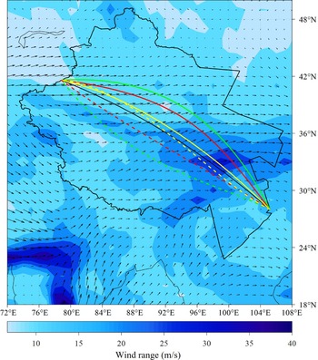
in characterising the uncertainty in trajectory flight time, a sensitivity analysis is conducted using a flight from Hong Kong International Airport (ICAO: VHHH) to Tel Aviv International Airport (ICAO: LLBG) as a case study. The entry and exit coordinates of the flight within CWA are
${{{\unicode{x03C8} }}_{f,0}}$
in characterising the uncertainty in trajectory flight time, a sensitivity analysis is conducted using a flight from Hong Kong International Airport (ICAO: VHHH) to Tel Aviv International Airport (ICAO: LLBG) as a case study. The entry and exit coordinates of the flight within CWA are $\left( {105.2^\circ E,28^\circ N} \right)$
and
$\left( {105.2^\circ E,28^\circ N} \right)$
and $\left( {78.8^\circ E,41.6^\circ N} \right)$
, respectively. The optimal lateral trajectories for the outbound (VHHH–LLBG) and return (LLBG–VHHH) flights are shown in Fig. 11, and the flight times are listed in Table 2.
$\left( {78.8^\circ E,41.6^\circ N} \right)$
, respectively. The optimal lateral trajectories for the outbound (VHHH–LLBG) and return (LLBG–VHHH) flights are shown in Fig. 11, and the flight times are listed in Table 2.
As shown in Table 2, the flight time of downwind flights (LLBG–VHHH) is shorter than that of upwind flights (VHHH–LLBG), primarily due to the prevailing subpolar westerlies over the airspace. The wind field presented in Fig. 11, which is averaged over four hours, reveals a region of high uncertainty spanning $31.5^\circ - 34.5^\circ N$
and
$31.5^\circ - 34.5^\circ N$
and $95^\circ - 103^\circ E$
. This wind pattern leads to several observable trajectory phenomena.
$95^\circ - 103^\circ E$
. This wind pattern leads to several observable trajectory phenomena.
When a higher level of reliability is required (i.e., a smaller value of ${{{\unicode{x03C8} }}_{f,0}}$
), the trajectories tend to circumvent regions with high uncertainty. Notably, the trajectories (solid lines) of VHHH–LLBG are more inclined to pass directly through the regions with high uncertainty, whereas the trajectories (dashed lines) of LLBG–VHHH are more likely to divert around them. This directional difference is primarily attributed to the time-variant nature of the wind field: the uncertainty within the region intensifies over time, such that it remains relatively weak when the VHHH–LLBG flights enter the area, but becomes significantly stronger by the time the LLBG–VHHH flights pass through. In addition, the solid lines tend to deviate northwards to avoid strong, unfavourable headwinds – particularly in the region between
${{{\unicode{x03C8} }}_{f,0}}$
), the trajectories tend to circumvent regions with high uncertainty. Notably, the trajectories (solid lines) of VHHH–LLBG are more inclined to pass directly through the regions with high uncertainty, whereas the trajectories (dashed lines) of LLBG–VHHH are more likely to divert around them. This directional difference is primarily attributed to the time-variant nature of the wind field: the uncertainty within the region intensifies over time, such that it remains relatively weak when the VHHH–LLBG flights enter the area, but becomes significantly stronger by the time the LLBG–VHHH flights pass through. In addition, the solid lines tend to deviate northwards to avoid strong, unfavourable headwinds – particularly in the region between $81^\circ E$
and
$81^\circ E$
and $89^\circ E$
indicated by the green solid line – while dashed lines are more likely to take advantage of favourable tailwinds to shorten time, as illustrated by the yellow dashed line between
$89^\circ E$
indicated by the green solid line – while dashed lines are more likely to take advantage of favourable tailwinds to shorten time, as illustrated by the yellow dashed line between $80.2^\circ E$
and
$80.2^\circ E$
and $86^\circ E$
. These results demonstrate that the proposed model is sensitive to the parameter
$86^\circ E$
. These results demonstrate that the proposed model is sensitive to the parameter ${{{\unicode{x03C8} }}_{f,0}}$
, and effectively captures the influence of time-variant wind forecast uncertainty, indicating its potential for application in lateral trajectory planning.
${{{\unicode{x03C8} }}_{f,0}}$
, and effectively captures the influence of time-variant wind forecast uncertainty, indicating its potential for application in lateral trajectory planning.
4.3.2 Efficiency analysis of
${Z_{ED}}$

In the lower-level model, this study aims to minimise ${Z_{ED}}$
, thereby reducing total delay while maintaining fairness among flights. To evaluate the effectiveness of this objective, two commonly used strategies are selected for comparative analysis: minimising the mean delay time (
${Z_{ED}}$
, thereby reducing total delay while maintaining fairness among flights. To evaluate the effectiveness of this objective, two commonly used strategies are selected for comparative analysis: minimising the mean delay time ( ${\mu _D}$
) and minimising the delay range (
${\mu _D}$
) and minimising the delay range ( ${\delta _D}$
). Table 3 presents the average values of
${\delta _D}$
). Table 3 presents the average values of ${\mu _D}$
and
${\mu _D}$
and ${\delta _D}$
obtained from 20 independent runs for each strategy, based on the corresponding solutions with the minimum number of conflicts. To further validate the robustness of the proposed fairness measure
${\delta _D}$
obtained from 20 independent runs for each strategy, based on the corresponding solutions with the minimum number of conflicts. To further validate the robustness of the proposed fairness measure ${Z_{ED}}$
, the Gini coefficient (
${Z_{ED}}$
, the Gini coefficient ( $\boldsymbol{\mathcal{G}}$
) is also evaluated using the existing optimisation results. This indictor quantifies the overall dispersion and relative inequality of flight delays, providing complementary insight into fairness performance. As constraint (20) remains identical across all experiments, the number of conflicts in the minimum-conflict solutions is the same for all three strategies, ensuring comparability of results.
$\boldsymbol{\mathcal{G}}$
) is also evaluated using the existing optimisation results. This indictor quantifies the overall dispersion and relative inequality of flight delays, providing complementary insight into fairness performance. As constraint (20) remains identical across all experiments, the number of conflicts in the minimum-conflict solutions is the same for all three strategies, ensuring comparability of results.
Comparison of delay performance under different optimisation strategies; results are averaged over 20 independent runs

Extremes of ${\mu _D}$
and
${\mu _D}$
and ${\delta _D}$
for each strategy; results are averaged over 20 independent runs
${\delta _D}$
for each strategy; results are averaged over 20 independent runs

Table 3 shows that when the strategy of minimising ${\mu _D}$
is adopted, the expected value
${\mu _D}$
is adopted, the expected value $E\left( {{\mu _D}} \right)$
is the lowest among the three strategies, indicating high efficiency in reducing average delay. However, this strategy also produces the highest values of
$E\left( {{\mu _D}} \right)$
is the lowest among the three strategies, indicating high efficiency in reducing average delay. However, this strategy also produces the highest values of ${\delta _D}$
and
${\delta _D}$
and $\boldsymbol{\mathcal{G}}$
, suggesting poor fairness among flights. In contrast, the strategy of minimising
$\boldsymbol{\mathcal{G}}$
, suggesting poor fairness among flights. In contrast, the strategy of minimising ${\delta _D}$
yields the lowest
${\delta _D}$
yields the lowest ${\delta _D}$
and
${\delta _D}$
and $\boldsymbol{\mathcal{G}}$
, representing the fairest outcome, but at the cost of increased average delay. Conversely, the strategy of minimising
$\boldsymbol{\mathcal{G}}$
, representing the fairest outcome, but at the cost of increased average delay. Conversely, the strategy of minimising ${Z_{ED}}$
achieves a balanced result, with both
${Z_{ED}}$
achieves a balanced result, with both ${\mu _D}$
,
${\mu _D}$
, ${\delta _D}$
, and
${\delta _D}$
, and $\boldsymbol{\mathcal{G}}$
values close to the optimal levels of the other two strategies. These results confirm that the proposed
$\boldsymbol{\mathcal{G}}$
values close to the optimal levels of the other two strategies. These results confirm that the proposed ${Z_{ED}}$
-based objective effectively reduces total delay while ensuring an equitable distribution of delay across flights.
${Z_{ED}}$
-based objective effectively reduces total delay while ensuring an equitable distribution of delay across flights.
Optimised lateral trajectories for flights VHHH–LLBG (solid lines) and LLBG–VHHH (dashed lines) under different ${{{\unicode{x03C8} }}_{f,0}}$
:
${{{\unicode{x03C8} }}_{f,0}}$
: ${{{\unicode{x03C8} }}_{f,0}} = 3$
(green),
${{{\unicode{x03C8} }}_{f,0}} = 3$
(green), ${{{\unicode{x03C8} }}_{f,0}} = 5$
(red),
${{{\unicode{x03C8} }}_{f,0}} = 5$
(red), ${{{\unicode{x03C8} }}_{f,0}} = 10$
(yellow).
${{{\unicode{x03C8} }}_{f,0}} = 10$
(yellow).

Table 4 gives the extreme values of ${\mu _D}$
and
${\mu _D}$
and ${\delta _D}$
across 20 independent runs under each strategy. When minimising
${\delta _D}$
across 20 independent runs under each strategy. When minimising ${\mu _D}$
, the value of
${\mu _D}$
, the value of ${\mu _D}$
remains relatively stable, but
${\mu _D}$
remains relatively stable, but ${\delta _D}$
varies considerably, indicating difficulty in consistently ensuring fairness. Similarly, minimising
${\delta _D}$
varies considerably, indicating difficulty in consistently ensuring fairness. Similarly, minimising ${\delta _D}$
results in greater variability in
${\delta _D}$
results in greater variability in ${\mu _D}$
, reflecting a trade-off in efficiency. However, the
${\mu _D}$
, reflecting a trade-off in efficiency. However, the ${Z_{ED}}$
-based strategy maintains both indicators within a narrow range, highlighting its robustness in achieving both delay reduction and fairness. These results further reinforce the practical value of the proposed objective function in multi-flight trajectory optimisation scenarios.
${Z_{ED}}$
-based strategy maintains both indicators within a narrow range, highlighting its robustness in achieving both delay reduction and fairness. These results further reinforce the practical value of the proposed objective function in multi-flight trajectory optimisation scenarios.
4.3.3 Efficiency analysis of SE strategy
To access the computational efficiency and convergence of the SE-based TVA*, a comparative analysis was conducted against the distance-based TVA*. Figure 12(a) presents the optimal trajectories obtained by both algorithms under ${{{\unicode{x03C8} }}_{f,0}} = 5$
. As illustrated, the green line generated by the distance-based TVA* algorithm more closely follows the great circle path. However, despite its shorter distance, the corresponding flight time is longer, reaching 2.85 h. This is primarily attributed to the limited sensitivity of the distance-based TVA* to uncertainty, which leads it to favour a shorter route while failing to account for the adverse effects of headwinds. In contrast, the SE-based TVA* effectively incorporates time-variant wind forecast uncertainty and exhibits superior capability in mitigating the impact of unfavourable wind conditions. These results confirm the exceptional efficiency of the SE strategy.
${{{\unicode{x03C8} }}_{f,0}} = 5$
. As illustrated, the green line generated by the distance-based TVA* algorithm more closely follows the great circle path. However, despite its shorter distance, the corresponding flight time is longer, reaching 2.85 h. This is primarily attributed to the limited sensitivity of the distance-based TVA* to uncertainty, which leads it to favour a shorter route while failing to account for the adverse effects of headwinds. In contrast, the SE-based TVA* effectively incorporates time-variant wind forecast uncertainty and exhibits superior capability in mitigating the impact of unfavourable wind conditions. These results confirm the exceptional efficiency of the SE strategy.
Comparison between the SE-based and distance-based TVA* algorithms, and the initial conflict distribution under ${{{\unicode{x03C8} }}_{f,0}} = 5$
: (a) optimal lateral trajectory of flight VHHH–LLBG: SE-based TVA* (red) versus distance-based TVA* (green); (b) initial optimal trajectories of all flights within the CWA, with potential conflicts indicated.
${{{\unicode{x03C8} }}_{f,0}} = 5$
: (a) optimal lateral trajectory of flight VHHH–LLBG: SE-based TVA* (red) versus distance-based TVA* (green); (b) initial optimal trajectories of all flights within the CWA, with potential conflicts indicated.

The flight time of the optimal trajectory calculated by GA is 2.72 h, which is identical to that produced by the SE-based TVA*, thereby demonstrating the convergence of the proposed algorithm. Regarding computational performance, the GA requires 32 s to compute a single trajectory, whereas the SE-based TVA* solves all 2,300 trajectories simultaneously in just 2.2 s, further validating its scalability and computational efficiency.
It is worth noting that the SE strategy is not strictly admissible or consistent under time-variant wind conditions, because the expected wind speed may slightly under- or over-estimate the true travel time of future segments when the wind field changes. Nevertheless, this does not affect the practical convergence behaviour of the algorithm. As demonstrated by the results above, the SE-based TVA* attains exactly the same optimal trajectory as the GA benchmark, while achieving a substantial reduction in computation time. These results confirm that the lack of strict admissibility has negligible practical impact on the solution quality, and the SE-based TVA* remains both reliable and highly efficient in the time-variant setting considered in this study.
The average solution time of MOCCEA based on EG, RG, DG and DEG strategies (min); results are averaged over 20 independent runs

4.3.4 Efficiency analysis of DEG strategy
The effectiveness of the DEG strategy is compared with three representative existing grouping methods: equilibrium grouping (EG), random grouping (RG), and dynamic grouping (DG) [Reference Guan, Zhang, Lv, Chen and Michal16] across four different traffic scenarios. The number of flights in each scenario varies due to differences in the time span: 465 flights (08:00–09:00), 949 flights (08:00–10:00), 1,708 flights (08:00–11:00) and 2,300 flights (08:00–12:00), respectively. Figure 12(b) illustrates the distribution of the initial optimal trajectories and conflict locations for the 2,300-flight scenario. The red lines denote the trajectories, while the yellow markers indicate the detected conflicts. A total of 2,182 conflicts have been identified, predominantly concentrated in the eastern and northern regions of the airspace, where traffic density is highest.
Table 5 presents the average solution times for each strategy, based on 20 independent runs. The results indicate that DEG consistently outperforms the other methods, with the most pronounced advantage observed in large-scale problems. This performance gain can be attributed to the high degree of coupling among large flights, which complicates the balanced allocation of computational load across CPU threads, thereby limiting the full parallel efficiency of MOCCEA.
The efficiency and convergence analysis: (a) the size of the largest group and the number of groups during the optimisation process of the DG strategy where $n = 2,300$
; (b) the IGD trends of the DEG-based MOCCEA across the four scenarios.
$n = 2,300$
; (b) the IGD trends of the DEG-based MOCCEA across the four scenarios.

To further illustrate this issue, Fig. 13(a) presents the evolution of the maximum group size and the number of groups during the optimisation process of the DG strategy for the case where $n = 2,300$
. The DG strategy performs grouping based solely on pairwise flight conflict relationships, without considering computational load balancing. As the algorithm proceeds, the size of the largest group gradually decreases, while the number of groups tends to increase. This trend reflects the reduction in conflict density, as more flights become conflict-free and interdependencies are weakened. However, groups containing only a single flight persist throughout the process. Although they no longer contribute significantly to optimisation, they consume computational resources, reducing overall efficiency. The DEG strategy effectively addresses this limitation by incorporating conflict structure and load balancing into the grouping process. For the largest scenario with 2,300 flights, the DEG strategy reduces the computation time to 42.28 min, achieving speed-ups of 1.42× over EG (60.08 min), 1.23× over RG (52.03 min), and 1.16× over DG (49.22 min).
$n = 2,300$
. The DG strategy performs grouping based solely on pairwise flight conflict relationships, without considering computational load balancing. As the algorithm proceeds, the size of the largest group gradually decreases, while the number of groups tends to increase. This trend reflects the reduction in conflict density, as more flights become conflict-free and interdependencies are weakened. However, groups containing only a single flight persist throughout the process. Although they no longer contribute significantly to optimisation, they consume computational resources, reducing overall efficiency. The DEG strategy effectively addresses this limitation by incorporating conflict structure and load balancing into the grouping process. For the largest scenario with 2,300 flights, the DEG strategy reduces the computation time to 42.28 min, achieving speed-ups of 1.42× over EG (60.08 min), 1.23× over RG (52.03 min), and 1.16× over DG (49.22 min).
As discussed in Section 4.3.3, the SE-based TVA* requires only 2.2 s to compute all 2,300 trajectories, accounting for less than 1% of the total solution time. The DEG-based MOCCEA dominates the overall computational cost owing to the large-scale conflict detection and resolution process. In serial execution, solving the entire bi-level optimisation problem takes approximately 266.4 min, whereas the parallel implementation using eight threads on an eight-core CPU reduces the total computation time to 42.28 min, achieving an average speed-up of 6.3×. These results clearly demonstrate that the proposed parallel framework substantially enhances computational efficiency and scalability, making it well-suited for large-scale strategic trajectory planning applications.
Figure 13(b) illustrates the IGD convergence trend of the DEG-based MOCCEA across the four scenarios, showing that the algorithm typically converges within approximately 120 generations. These findings confirm that the DEG-based MOCCEA is convergent and significantly improves computational efficiency, particularly in large-scale, high-density traffic scenarios.
Figure 14 presents the Pareto fronts for the four scenarios under comparison. Across all scenarios, the DEG strategy consistently produces superior Pareto fronts compared to the other strategies, demonstrating its overall advantage. Specifically, the DG strategy increases the number of groups during the conflict resolution process, which results in additional computational overhead. The EG strategy, by contrast, overlooks the coupling relationships among flights, leading to inefficient grouping and reduced performance. In comparison, the DEG strategy effectively balances computational loads across threads while preserving critical conflict structures, enhancing both the final solutions’ efficiency and quality.
To better emphasise the methodological contribution of the proposed DEG strategy, Table 6 presents a comparative analysis with the EG, RG and DG methods. Unlike EG and RG, which are static in nature, or DG, which groups flights solely according to conflict relationships, the proposed DEG method integrates both conflict awareness and thread load balancing. This dual consideration enables DEG to maintain near-uniform computational workloads across threads while preserving critical inter-flight conflict structures, thereby achieving superior scalability and parallel efficiency in large-scale optimisation.
Comparison between DEG and existing grouping strategies

4.3.5 Evaluation of the bi-level STP framework
To demonstrate the advantages of the proposed bi-level planning model, this section compares the optimal Pareto fronts generated by the bi-level model and the two-stage model under four traffic scenarios, as illustrated in Fig. 15. The results show that, across all scenarios, the Pareto fronts obtained from the bi-level model consistently dominate those of the two-stage approach. This performance gain is primarily attributed to the inherent limitations of the two-stage model: under time-variant wind conditions, adjusting departure times during the second stage may render the lateral trajectories optimised for the first stage suboptimal. Moreover, changes in departure times reduce the predictability of aircraft arrival times at trajectory sampling points, making it difficult to accurately detect and resolve potential conflicts. In contrast, the bi-level model accounts for the coupling between trajectory planning and conflict resolution, thereby effectively addressing these issues.
Average solution time (min) of the two-stage model and bi-level models across four traffic scenarios (8 CPU threads); results are averaged over 20 independent runs

The Pareto front of the EG, RG, DG and DEG strategies for four scenarios: (a) $n = 465$
; (b)
$n = 465$
; (b) $n = 949$
; (c)
$n = 949$
; (c) $n = 1,708$
; (d)
$n = 1,708$
; (d) $n = 2,300$
.
$n = 2,300$
.

The Pareto fronts of the two-stage model and bi-level model for four scenarios: (a) $n = 465$
; (b)
$n = 465$
; (b) $n = 949$
; (c)
$n = 949$
; (c) $n = 1,708$
; (d)
$n = 1,708$
; (d) $n = 2,300$
.
$n = 2,300$
.

Table 7 shows the computation times for both the two-stage and bi-level models across the four scenarios. As the number of flights increases, the bi-level model exhibits increasingly better performance compared with the two-stage model, highlighting its scalability and robustness in handling large-scale optimisation. These results confirm that the proposed approach is both practical and effective for strategic trajectory planning, with strong potential to enhance the overall efficiency of air traffic management.
5.0 Conclusion
This study addresses the large-scale strategic trajectory planning problem under time-variant wind forecast uncertainty by proposing a bi-level optimisation model. The upper-level model minimises total flight time within an acceptable uncertainty bound, while the lower-level model mitigates conflicts and departure delays with an emphasis on fairness. A novel delay-fairness objective function, ${Z_{ED}}$
, is introduced to balance delay reduction and fairness. In addition, an integrated algorithmic framework is developed, combining SE-based TVA* and DEG-based MOCCEA to improve search directionality and parallel computation efficiency.
${Z_{ED}}$
, is introduced to balance delay reduction and fairness. In addition, an integrated algorithmic framework is developed, combining SE-based TVA* and DEG-based MOCCEA to improve search directionality and parallel computation efficiency.
Extensive numerical experiments demonstrate that the proposed bi-level framework consistently outperforms traditional two-stage approaches, yielding dominant Pareto fronts across multiple traffic scenarios. The model improves flight efficiency, ensures operational safety and maintains fairness, providing tangible value for large-scale STP in ATM systems characterised by high traffic density and time-variant wind forecast uncertainty. From an operational perspective, the proposed bi-level STP framework could be integrated into the pre-tactical or strategic planning stages of ATM. Within an FRA environment, the upper-level can generate route options that comply with sector boundaries, airspace availability and NOTAM restrictions. The lower-level can then feed these optimised trajectories into existing tactical conflict detection and resolution tools, supporting air traffic controllers in real-time decision-making. In this way, the proposed framework can act as an upstream decision-support module, bridging strategic and tactical operations to enhance overall system efficiency and safety.
Despite its promising results, this study has several limitations. The wind forecast uncertainty is currently represented as a piecewise function, which may limit its ability to capture fine-grained variability. Future work will explore continuous modelling approaches to improve trajectory prediction accuracy. Moreover, the current study focuses exclusively on lateral trajectory planning; incorporating vertical optimisation, such as altitude adjustment, remains a promising direction. Finally, the model has thus far been evaluated only through simulation. A key avenue for future work is to validate the framework with operational flight data and integrate it with real-world ATM systems to assess its practical applicability fully.
Acknowledgements
This research is supported by the National Natural Science Foundation of China under Grant (No. 52472340), the National Key Research and Development Program of China (No.2021YFB1600100), the SEU Innovation Capability Enhancement Plan for Doctoral Students (CXJH_SEU25179), and the Big Data Computing Centre of Southeast University.
Code and data availability
The wind-field data used in this study are obtained from the ECMWF ERA5 reanalysis. The trajectory datasets and optimisation parameters used in the experiments are derived from the China Western Airspace (CWA) operational environment as described in the manuscript. The MATLAB implementation of the proposed framework, together with the processed input data, is available from the authors upon reasonable request for academic research purposes.
Appendix A. Sensitivity to forced segment splitting at TVMs
To assess the potential error introduced by not splitting a segment when it crosses a TVM, a small-scale verification experiment was conducted. A sample of 100 trajectories was randomly selected from the flight ensemble. For each trajectory, the travel time and number of conflicts were recomputed under two configurations:
-
(1) Baseline: each segment applies the wind field corresponding to its start time window without splitting at TVMs.
-
(2) Forced-split: segments intersecting a TVM are divided at the boundary, and the corresponding sub-segments use the wind of their respective time windows.
The results show that forcing a split changes the average flight time ( $E\left( T \right)$
) by less than ±0.3% and the total number of conflicts (
$E\left( T \right)$
) by less than ±0.3% and the total number of conflicts ( ${Z_{CN}}$
) by less than ±0.5%. The maximum deviation in single-flight travel time was 0.8%. These findings indicate that the baseline treatment introduces only a negligible bias, while avoiding the additional computational.
${Z_{CN}}$
) by less than ±0.5%. The maximum deviation in single-flight travel time was 0.8%. These findings indicate that the baseline treatment introduces only a negligible bias, while avoiding the additional computational.
Appendix B. Sensitivity analysis on wind update interval (
${t_v}$
) and grid resolution (
$\Delta $
)


Since the average flight time $E\left( T \right)$
and conflict number
$E\left( T \right)$
and conflict number ${Z_{CN}}$
do not have absolute benchmark values, we used a relative evaluation approach. The reference solution was generated using finest feasible configuration based on a dataset of 2,300 flights. We take
${Z_{CN}}$
do not have absolute benchmark values, we used a relative evaluation approach. The reference solution was generated using finest feasible configuration based on a dataset of 2,300 flights. We take $t_v^{{\rm{ref}}} = 0.5\;{\rm{h}}$
and
$t_v^{{\rm{ref}}} = 0.5\;{\rm{h}}$
and ${\Delta ^{{\rm{ref}}}} = 0.1^\circ $
(finest feasible in our setup) as the reference discretisation and denote the corresponding outputs by
${\Delta ^{{\rm{ref}}}} = 0.1^\circ $
(finest feasible in our setup) as the reference discretisation and denote the corresponding outputs by $E{\left( T \right)^{{\rm{ref}}}}$
and
$E{\left( T \right)^{{\rm{ref}}}}$
and $Z_{CN}^{{\rm{ref}}}$
. We then vary
$Z_{CN}^{{\rm{ref}}}$
. We then vary ${t_v} \in \left\{ {0.5,1.0,1.5,2.0} \right\}{\rm{\;h}}$
and
${t_v} \in \left\{ {0.5,1.0,1.5,2.0} \right\}{\rm{\;h}}$
and $\Delta \in \left\{ {0.1^\circ ,0.2^\circ ,0.3^\circ ,0.4^\circ } \right\}$
and report (1) the relative error to the reference, and (2) the corresponding runtime. The relative error is defined as follows:
$\Delta \in \left\{ {0.1^\circ ,0.2^\circ ,0.3^\circ ,0.4^\circ } \right\}$
and report (1) the relative error to the reference, and (2) the corresponding runtime. The relative error is defined as follows:
 \begin{align}{\rm{RelEr}}{{\rm{r}}_T} = \frac{{\left| {E\left( T \right) - E{{(T)}^{{\rm{ref}}}}} \right|}}{{E{{(T)}^{{\rm{ref}}}}}} \times 100{\rm{\% }} \\[-28 pt] \nonumber \end{align}
 \begin{align}{\rm{RelEr}}{{\rm{r}}_{CN}} = \frac{{\left| {{Z_{CN}} - Z_{CN}^{{\rm{ref}}}} \right|}}{{Z_{CN}^{{\rm{ref}}}}} \times 100{\rm{\% }} \\[6pt] \nonumber \end{align}
We choose the coarsest $\left( {{t_v},\Delta } \right)$
that satisfies
$\left( {{t_v},\Delta } \right)$
that satisfies ${\rm{RelEr}}{{\rm{r}}_T} \le 0.5\% $
and
${\rm{RelEr}}{{\rm{r}}_T} \le 0.5\% $
and ${\rm{RelEr}}{{\rm{r}}_{CN}} \le 0.5\% $
, while maximising speed-up. This reflects the operational priority of keeping trajectory-cost bias small and not missing conflicts, without incurring unnecessary runtime. The results are concluded in Table B1.
${\rm{RelEr}}{{\rm{r}}_{CN}} \le 0.5\% $
, while maximising speed-up. This reflects the operational priority of keeping trajectory-cost bias small and not missing conflicts, without incurring unnecessary runtime. The results are concluded in Table B1.
Sensitivity analysis to wind update interval ( ${t_v}$
) and grid resolution (
${t_v}$
) and grid resolution ( $\Delta $
)
$\Delta $
)

Using the stricter criteria ${\rm{RelEr}}{{\rm{r}}_{\rm{T}}} \le 0.5{\rm{\% }}$
and
${\rm{RelEr}}{{\rm{r}}_{\rm{T}}} \le 0.5{\rm{\% }}$
and ${\rm{RelEr}}{{\rm{r}}_{{\rm{CN}}}} \le 0.5{\rm{\% }}$
, the admissible configurations are:
${\rm{RelEr}}{{\rm{r}}_{{\rm{CN}}}} \le 0.5{\rm{\% }}$
, the admissible configurations are: $\left( {0.5{\rm{\;h}},0.1^\circ } \right)$
,
$\left( {0.5{\rm{\;h}},0.1^\circ } \right)$
, $\left( {0.5{\rm{\;h}},0.2^\circ } \right)$
,
$\left( {0.5{\rm{\;h}},0.2^\circ } \right)$
, $\left( {1{\rm{\;h}},0.1^\circ } \right)$
,
$\left( {1{\rm{\;h}},0.1^\circ } \right)$
, $\left( {1{\rm{\;h}},0.2^\circ } \right)$
and
$\left( {1{\rm{\;h}},0.2^\circ } \right)$
and $\left( {1.5{\rm{\;h}},0.1^\circ } \right)$
. Among these,
$\left( {1.5{\rm{\;h}},0.1^\circ } \right)$
. Among these, $\left( {1{\rm{\;h}},0.2^\circ } \right)$
achieves the lowest runtime (42.28 min, normalised to the reference) while exactly meeting the time-error bound (0.5%) and remaining within the conflict-error bound (0.4%). Coarsening beyond
$\left( {1{\rm{\;h}},0.2^\circ } \right)$
achieves the lowest runtime (42.28 min, normalised to the reference) while exactly meeting the time-error bound (0.5%) and remaining within the conflict-error bound (0.4%). Coarsening beyond $0.2^\circ $
or increasing the update interval beyond 1 h violates at least one threshold, whereas finer settings bring negligible accuracy gains at substantially higher cost. Hence,
$0.2^\circ $
or increasing the update interval beyond 1 h violates at least one threshold, whereas finer settings bring negligible accuracy gains at substantially higher cost. Hence, $\left( {1{\rm{\;h}},0.2^\circ } \right)$
is the preferred operating point – an elbow that preserves accuracy under the 0.5% limits and maximises speed-up.
$\left( {1{\rm{\;h}},0.2^\circ } \right)$
is the preferred operating point – an elbow that preserves accuracy under the 0.5% limits and maximises speed-up.
Appendix C. Sensitivity of four-dimensional sampling distance
To examine how the spatial sampling distance ( ${\rm{\Delta }}d$
) affects conflict detection accuracy and computational performance, a sensitivity analysis was performed using a dataset of 2,300 flights. The sampling distance was varied between 1 and 10 km (
${\rm{\Delta }}d$
) affects conflict detection accuracy and computational performance, a sensitivity analysis was performed using a dataset of 2,300 flights. The sampling distance was varied between 1 and 10 km ( ${\rm{\Delta }}d = \left\{ {1,2,3,4,5,6,7,8,9,10} \right\}$
km). The finest resolution (
${\rm{\Delta }}d = \left\{ {1,2,3,4,5,6,7,8,9,10} \right\}$
km). The finest resolution ( ${\rm{\Delta }}d = 1$
km) served as the reference case. Two key performance metrics were examined: (1) the number of initially detected conflicts; and (2) the corresponding detection time. The results are summarised in Table C1.
${\rm{\Delta }}d = 1$
km) served as the reference case. Two key performance metrics were examined: (1) the number of initially detected conflicts; and (2) the corresponding detection time. The results are summarised in Table C1.
Sensitivity of conflict detection and runtime to spatial sampling distance

As shown in Table C1, when the sampling distance ( ${\rm{\Delta }}d$
) is less than or equal to 5 km, the number of initially detected conflicts remains constant at 2,182, indicating that the conflict detection results are insensitive to further refinement. Beyond this threshold, the number of detected conflicts decreases rapidly, suggesting that a coarser spatial resolution leads to missed short-range conflicts. Meanwhile, the detection time decreases almost linearly with increasing
${\rm{\Delta }}d$
) is less than or equal to 5 km, the number of initially detected conflicts remains constant at 2,182, indicating that the conflict detection results are insensitive to further refinement. Beyond this threshold, the number of detected conflicts decreases rapidly, suggesting that a coarser spatial resolution leads to missed short-range conflicts. Meanwhile, the detection time decreases almost linearly with increasing ${\rm{\Delta }}d$
, dropping from 1.86 s at 1 km to 0.24 s at 10 km. Therefore, a sampling distance of 5 km provides an appropriate balance between detection accuracy and computational efficiency, ensuring reliable conflict identification while maintaining fast runtime.
${\rm{\Delta }}d$
, dropping from 1.86 s at 1 km to 0.24 s at 10 km. Therefore, a sampling distance of 5 km provides an appropriate balance between detection accuracy and computational efficiency, ensuring reliable conflict identification while maintaining fast runtime.