

Introduction
Sea-level change is one of the most well-known consequences of climate change. Rising sea levels will impact coastal populations all around the world (Nicholls & Cazenave, Reference Nicholls and Cazenave2010) and increase the frequency and magnitude of high water levels (Wahl et al., Reference Wahl, Haigh, Nicholls, Arns, Dangendorf, Hinkel and Slangen2017). Understanding and projecting sea-level rise is therefore important for low-lying countries such as the Netherlands. It is of specific interest for vulnerable coastal wetland regions, such as the Wadden Sea World Heritage area, since even small external changes may disturb the system's delicate equilibrium (Kirwan & Megonigal, Reference Kirwan and Megonigal2013).
Global mean sea level (GMSL) has been rising at a rate of c.3mma−1 since 1993 (e.g. Chen et al., Reference Chen, Zhang, Church, Watson, King, Monselesan, Legresy and Harig2017). GMSL changes are defined as changes in the total volume of the oceans. These changes are ultimately caused by two processes: changes in the total mass of the ocean and changes in the density of ocean waters. Regionally, sea-level change can deviate substantially from the global mean change. These regional changes take place over a wide range of spatial and temporal scales and are driven by many different processes. In the first section of this paper, we discuss the major drivers of sea-level variability in global mean, and in the North Sea and Wadden Sea over decadal to centennial timescales.
In the second section of this paper, we present available observations of sea-level change in the North Sea and Wadden Sea area. This includes sea-level index points which can be used to reconstruct sea-level change on palaeo-timescales, as well as present-day instrumental records of sea-level change by satellites and tide gauges. Observations of global mean sea-level change are discussed in the Appendix.
Projections of global and regional sea-level change in the Wadden Sea area up to the year 2100 are presented in the third section of this paper. The regional sea-level projections from the Intergovernmental Panel on Climate Change Fifth Assessment Report (IPCC AR5; Church et al., Reference Church, Clark, Cazenave, Gregory, Jevrejeva, Levermann, Merrifield, Milne, Nerem, Nunn, Payne, Pfeffer, Stammer, Unnikrishnan, Stocker, Qin, Plattner, Tignor, Allen, Boschung, Nauels, Xia, Bex and Midgley2013) are taken as the starting point of this assessment. These projections include ocean steric and dynamic changes, ice sheet and glacier mass changes, changes in land-water storage due to groundwater extraction, atmospheric pressure change and glacial isostatic adjustment (GIA). The influence of recent advances in sea-level change research on the regional projections for the Wadden Sea will be assessed.
Research gaps and potential ways forward to improve understanding and projections of sea-level change in the Wadden Sea area are presented in the Discussion section, followed by a summary of the main findings in the Conclusions section.
Unless indicated otherwise, sea-level changes presented in this paper are so-called relative sea-level (RSL) changes, which is the difference between the ocean surface and the ocean floor, i.e. the depth of the water column. This is different from the absolute sea-level change, which is the difference between the ocean surface and the Earth's centre of mass.
Causes of global and regional sea-level change
Global mean sea-level change processes
Changes in ocean mass
Since the total amount of water at the Earth's surface is roughly constant in time, changes in ocean mass are mirrored by changes in the amount of water stored on land and in the atmosphere (Gregory et al., Reference Gregory, White, Church, Bierkens, Box, van den Broeke, Cogley, Fettweis, Hanna, Huybrechts, Konikow, Leclercq, Marzeion, Oerlemans, Tamisiea, Wada, Wake and van de Wal2013). A large fraction of land water is stored as ice in glaciers and in the Greenland and Antarctic Ice Sheets. In addition, land water is also stored in lakes and rivers, in underground aquifer systems, and at the surface in the form of soil moisture and snow. The total amount of fresh water stored in the atmosphere is only 0.04% of the fresh water stored on land (Gleick, Reference Gleick1996) and its contribution is usually ignored when assessing long-term ocean mass changes.
At seasonal timescales, ocean mass changes are mainly due to changes in precipitation, river discharge and evaporation. At annual and longer timescales, the major processes driving mass redistribution between land and the oceans are ice mass changes from glaciers and the ice sheets (Shepherd et al., Reference Shepherd2012; Gardner et al., Reference Gardner, Moholdt, Cogley, Wouters, Arendt, Wahr and Ligtenberg2013), as well as long-term trends in terrestrial water storage (Wada et al., Reference Wada, van Beek, van Kempen, Reckman, Vasak and Bierkens2010; Konikow, Reference Konikow2011). The latter is primarily caused by direct human interventions, such as groundwater mining and dam building (Church et al., Reference Church, Clark, Cazenave, Gregory, Jevrejeva, Levermann, Merrifield, Milne, Nerem, Nunn, Payne, Pfeffer, Stammer, Unnikrishnan, Stocker, Qin, Plattner, Tignor, Allen, Boschung, Nauels, Xia, Bex and Midgley2013).
Changes in ocean density
Global ocean volume changes are caused by density variations in sea water due to changes in temperature, also known as thermosteric changes (e.g. Johnson & Wijffels, Reference Johnson and Wijffels2011). Since the oceans absorb the vast majority of the heat excess in the Earth system, due to the capacity of water to store large amounts of thermal energy, they are becoming warmer and expanding, which results in GMSL rise. However, the oceans are not static and not warming uniformly: the actual spatial pattern of ocean volume changes is the result of the interaction between insulation, atmospheric temperature, winds, freshwater fluxes and ocean dynamics.
An overview of observations of global mean sea level, from the geological past to the satellite-era present, is given in the Appendix.
Sea-level change processes in the North Sea and Wadden Sea
Mass changes
Redistribution of water between land and ocean does not only result in a change of GMSL. Due to deformation of the solid earth as well as changes in the gravity field and the Earth rotation parameters, mass redistribution results in regionally varying sea-level patterns. Those patterns are known as ‘fingerprints’ (Farrell & Clark, Reference Farrell and Clark1976; Mitrovica et al., Reference Mitrovica, Tamisiea, Davis and Milne2001). The different sources of mass loss each have a distinct impact on regional sea level (Fig. 1). The black contours in Figure 1 indicate the global mean value: note that regions closer to the sources of ice-sheet mass loss show a rise below average (even a reduction in sea level in the first 2000km), while regions further away show an above-average rise. In the North Sea and Wadden Sea, sea-level changes as a result of mass loss of the ice sheets are below the global average (Table 1).
Impact of mass loss on regional sea level from glaciers and each ice sheet assuming a mass loss trend of 362Gt (or 362km3 of fresh water) per year, which equals a Global Mean Sea Level (GMSL) rise of 1 mma−1. The black line shows the 1mma−1 contour. The right panels depict a regional inset for the European coast. The impact has been computed using the elastic approximation of the sea-level equation (Tamisiea et al., Reference Tamisiea, Hill, Ponte, Davis, Velicogna and Vinogradova2010), together with the rotational feedback (Mitrovica et al., Reference Mitrovica, Wahr, Matsuyama and Paulson2005). The regional partitioning of ice mass loss over both ice sheets is based on GRACE observations (Watkins et al., Reference Watkins, Wiese, Yuan, Boening and Landerer2015) and for glaciers, based on the modelled regional mass loss from Marzeion et al. (Reference Marzeion, Leclercq, Cogley and Jarosch2015).
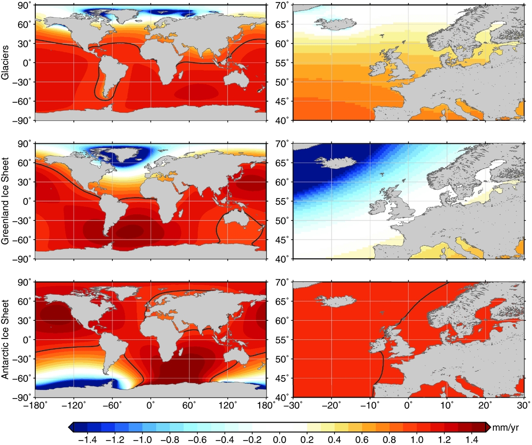
Ratio of sea-level changes in the North Sea to mass changes from glaciers, Greenland and Antarctica (Fig. 1). For the North Sea, the ratio at 56.25N, 3.75E has been used. For the Wadden Sea, the ratio at 53.25N, 5.25E has been used.

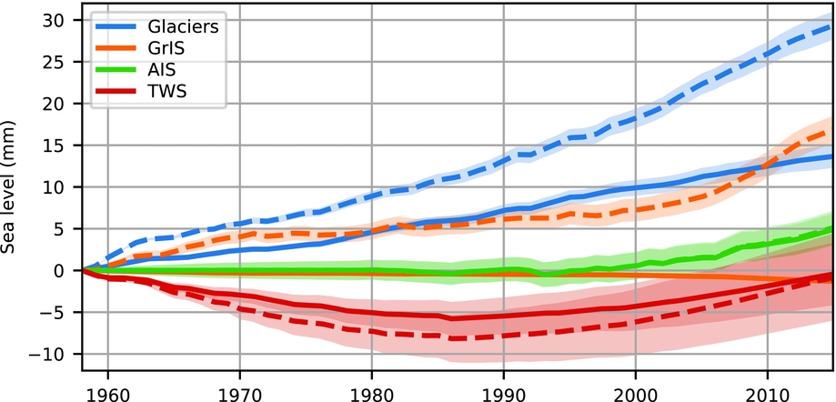
The regional sea-level fingerprints that result from mass redistribution caused by ice mass and land-water storage changes can be used to compute the effect of land-water mass redistribution on sea level in the North Sea (Fig. 2). Mass loss from glaciers and the Greenland Ice Sheet dominates global mean mass change initially, while the Antarctic Ice Sheet has only started to contribute significantly to the budget since the beginning of the 21st century (Fig. 2). However, due to the fact that Greenland and many glacierised regions are relatively close to the North Sea, their impact on local sea level is substantially smaller than their impact on the global mean.
Global mean (dashed) and local (solid) sea-level changes in the North Sea (56.25°N, 3.75°E) resulting from present-day mass redistribution processes over 1958–2014. GrIS denotes the Greenland Ice Sheet contribution, AIS the Antarctic Ice Sheet contribution, and TWS the contribution from terrestrial water storage (Frederikse et al., Reference Frederikse, Simon, Katsman and Riva2017). The shaded areas denote the confidence intervals at the 1σ level. The global and North Sea mean AIS contribution are almost equal (figure based on data from Frederikse et al., Reference Frederikse, Simon, Katsman and Riva2017)
Steric changes and ocean dynamics
In the open ocean, the vast majority of the dynamic sea-level signal on interannual and longer timescales is directly linked to local density changes (e.g. Forget & Ponte, Reference Forget and Ponte2015), which in the North Atlantic include shallow ocean-water sterics of the Gulf Stream, besides the northbound Southern Ocean intermediate waters and southbound North Atlantic deep waters of the thermohaline circulation. However, it becomes more complicated along a shallow continental shelf: since the water column in shallow water is small, the effect of local density changes becomes small as well. The increasing importance of local density changes when the water column becomes larger leads to lateral sea-level gradients that cause a transport of water from the open ocean onto the shelf (Landerer et al., Reference Landerer, Jungclaus and Marotzke2007).
However, sea level often shows coherent variability along the shoreline on interannual and longer timescales, and hence, this aforementioned shelf-sea response to open-ocean steric changes is not always a suitable approximation for on-shelf dynamic sea-level changes (Bingham & Hughes, Reference Bingham and Hughes2012). Alongshore wind forcing causes a substantial decadal variability signal along the European coast and the North Sea (Sturges & Douglas, Reference Sturges and Douglas2011). When the longshore wind direction points northward, Ekman transport drives surface waters towards the coast, which subsides at the coast, deepening the thermocline. This deepening of the thermocline results in higher sea level. These sea-level anomalies travel northward along the shelf edge as coastally trapped waves. Therefore, coastal sea level is highly correlated with changes in the alongshore wind, integrated from the equator to the European coast (Calafat et al., Reference Calafat, Chambers and Tsimplis2012). This signal travels northward along the Norwegian coast (Calafat et al., Reference Calafat, Chambers and Tsimplis2013) and also affects the North Sea (Dangendorf et al., Reference Dangendorf, Wahl, Nilson, Klein and Jensen2014b; Frederikse et al., Reference Frederikse, Riva, Slobbe, Broerse and Verlaan2016b). This anomaly is also found offshore, as westward-travelling Rossby waves result in open-ocean adjustment (Marcos et al., Reference Marcos, Puyol, Calafat and Woppelmann2013), which explains the open-ocean correlation with coastal sea level in the temperate-latitude North Atlantic.
At higher latitudes, the dynamic signal follows the topography gradient, resulting in a westward propagation towards the Subpolar North Atlantic (Hughes & Meredith, Reference Hughes and Meredith2006). Since the coastally trapped waves are predominantly baroclinic in nature (Calafat et al., Reference Calafat, Chambers and Tsimplis2012), the propagated signal can be extracted from temperature and salinity data recorded just offshore the European and Norwegian shelf (Marcos et al., Reference Marcos, Puyol, Calafat and Woppelmann2013; Dangendorf et al., Reference Dangendorf, Wahl, Nilson, Klein and Jensen2014b; Frederikse et al., Reference Frederikse, Riva, Kleinherenbrink, Wada, Broeke and Marzeion2016a).
The correlation between the decadal sea-level variability from tide gauges with altimetry (Fig. 3) confirms the presence of a large-scale coherent sea-level pattern along the Northwestern European Shelf. This large-scale coherent pattern can also be extracted from in situ temperature and salinity observations (Frederikse et al., Reference Frederikse, Riva, Kleinherenbrink, Wada, Broeke and Marzeion2016a). Density variations sampled at these locations give information not only on the decadal variability signal, related to alongshore wind forcing, but also about longer-term thermal expansion due to the increasing ocean heat content.
Correlation pattern between decadal variability, observed by tide gauges in the Wadden Sea (blue dot), and sea level observed by satellite altimetry in the North Atlantic. From the tide gauge time series the effects of wind and pressure have been removed, and the altimetry time series (ESA CCI, Legeais et al., Reference Legeais, Ablain, Zawadzki, Zuo, Johannessen, Scharffenberg, Fenoglio-Marc, Fernandes, Andersen, Rudenko, Cipollini, Quartly, Passaro, Cazenave and Benveniste2018) have been corrected for pressure (the inverted barometer effect). The correlation has been computed from detrended and low-pass filtered data using a 25-month moving average filter.

In addition to basin-wide sea-level changes related to wind-driven coastally trapped waves, internal dynamics in the North Sea result in intra-basin differences. These intra-basin variations have been studied qualitatively using a regional ocean model (Sterlini et al., Reference Sterlini, Le Bars, de Vries and Ridder2017). Similar to the open oceans, to maintain a zero pressure gradient at depth, local changes in the sea surface height in deep waters transmit a signal barotropically to shallower regions. Hence remote steric effects drive changes in the local sea level. These sea-level changes can be calculated by spatially integrating along an averaged density at a given depth from which remote steric changes are assumed to have a local influence (Bingham & Hughes, Reference Bingham and Hughes2012).
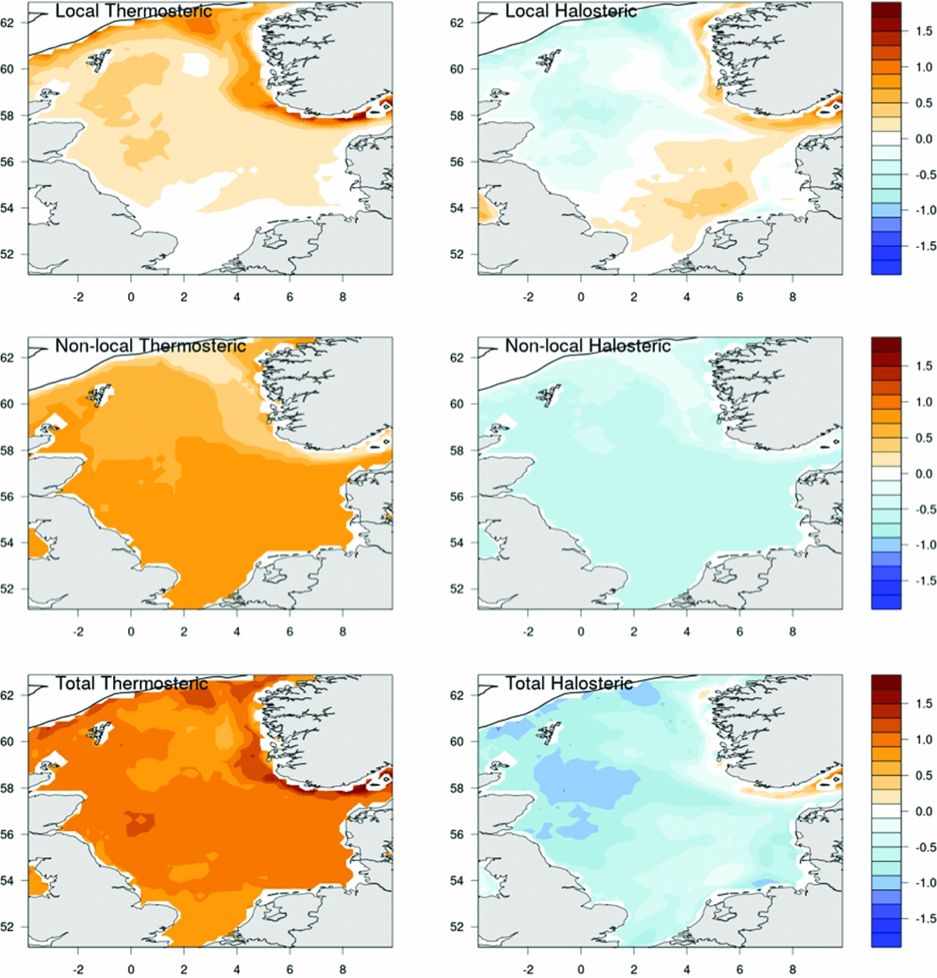
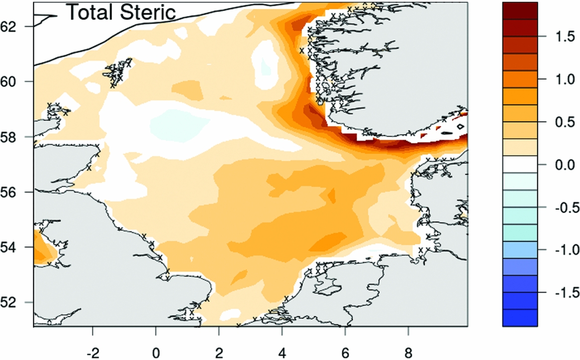
Hence, to obtain the total sea-level change due to steric effects, the local and remote components must be added together. These components are shown in Figure 4. Steric sea-level rise occurs over most of the North Sea (Fig. 5), with highest levels seen off the Norwegian coast (~1.5mma−1), attributable mostly to local thermo- and halosteric processes. Halosteric effects lead to a secondary region of high steric sea-level rise to the north of the Wadden Sea (~0.9mma−1).
Sea-level response to the thermosteric (left) and halosteric (right) effects in the North Sea, 1993–2013 (mma−1). Upper: local; Mid: non-local; Lower: total (local + non-local). Data beyond the 600m depth contour are not plotted. Crosses near the coast show regions where data are unavailable (Sterlini et al., Reference Sterlini, Le Bars, de Vries and Ridder2017).
Total steric sea-level response in the North Sea, 1993–2013 (mma−1). Data beyond the 600m depth contour are not plotted. Crosses show regions where data are unavailable (Sterlini et al., Reference Sterlini, Le Bars, de Vries and Ridder2017).
Nodal cycle
The 18.6-year nodal cycle is caused by a precessional motion of the lunar orbital plane with respect to the ecliptic (the orbital plane of the Earth around the Sun). As a result, the inclination of the lunar plane with respect to the equator varies over a cycle of 18.6 years.
This cycle has two distinct effects. On the one hand, it modulates the amplitude (and phase) of the lunar constituents, notably the principal semidiurnal lunar constituent M2 and lunar declinational diurnal constituents K1 and O1. This modulation has a significant effect on the tidal range and on the diurnal inequality, but it leaves the annual mean sea level unaffected since high waters are as much higher as low waters are lower, giving a cancellation in the mean. On the other hand, there is a small long-period nodal constituent N, which has no effect on the tidal range but does have a signature in annual mean sea level. This constituent has an equilibrium amplitude of c.7mm in the Wadden Sea (Woodworth, Reference Woodworth2012).
Since sea-level adjustment to changes in the tidal potential happens at substantially shorter timescales than the period of the nodal cycle, it is generally assumed that sea level follows the equilibrium tide at the lowest frequencies (Proudman, Reference Proudman1960). In the North Sea, this nodal signal is indeed found to stay close to tidal equilibrium over the past decades (Frederikse et al., Reference Frederikse, Riva, Slobbe, Broerse and Verlaan2016b). Since on decadal and multi-decadal timescales, sea-level variability in the North Sea and Wadden Sea shows strong coherence, the nodal cycle is likely to stay close to the equilibrium amplitude in the Wadden Sea as well.
Glacial isostatic adjustment
Glacial isostatic adjustment (GIA) is the process of ongoing changes to the growth and melt of large ice sheets on ice age timescales. Next to the almost-instantaneous elastic deformation of the solid earth following mass redistribution, viscous processes in the inner earth result in an ongoing deformation of the earth surface (McConnell, Reference McConnell1965; Farrell, Reference Farrell1972; Peltier & Andrews, Reference Peltier and Andrews1976; Lambeck, Reference Lambeck1990). During periods of glaciation, the solid earth subsides under the load of ice, and mantle material is pushed radially outwards. As a result, the peripheral area that surrounds the ice-sheet margin experiences uplift and generates the so-called peripheral forebulge. This process is inverted during deglaciations, the last one being the Last Glacial Maximum (LGM), and continues after the disappearance of ice. The rate at which GIA-induced deformation of the solid earth occurs is a function of the Earth's mantle viscosity and of the rigidity of the overlying elastic lithosphere and decay exponentially with time. The GIA process gives rise to regionally varying changes in seabed topography and related RSL changes that strongly deviate from the global mean changes as a function of the distance with respect to the ice sheets (Farrell & Clark, Reference Farrell and Clark1976; Mitrovica & Peltier, Reference Mitrovica and Peltier1991). Isostatic adjustment, or dynamic topography, also occurs due to mass shifting of ocean and shelf-sea waters, proglacial lake water and groundwater (hydro isostasy) and sedimentation (sediment isostasy).
Throughout the last 15,000 years, palaeo-sea-level indicators show a significant spatial variability of RSL changes across northwestern Europe (Lambeck et al., Reference Lambeck, Johnston and Nakada1990, Reference Lambeck, Smither and Johnston1998; Kiden et al., Reference Kiden, Denys and Johnston2002; Vink et al., Reference Vink, Steffen, Reinhardt and Kaufmann2007). This is a consequence of the growth and melting of the Fennoscandian Ice Sheet in the Last Glacial. In particular, sites from along the Baltic Sea and the Gulf of Bothnia show a significant RSL fall as a function of isostatic crustal uplift and decrease of ice-induced gravitational pull (e.g. Lambeck et al., Reference Lambeck, Johnston and Nakada1990, Reference Lambeck, Smither and Johnston1998).
The North Sea can be considered an ice-proximal area (i.e. near-field) with respect to the mass centres of the large Fennoscandian Ice Sheet, and the smaller ice sheet of the British Isles to the northwest (Denton & Hughes, Reference Denton and Hughes1981; Lambeck et al., Reference Lambeck, Johnston and Nakada1990; Ehlers & Gibbard, Reference Ehlers and Gibbard2003; Peltier, Reference Peltier2004). It is reasonable to assume that, during the LGM, the southerly ice-free areas of the North Sea and surroundings were uplifted as a consequence of the ice-loading that caused Fennoscandia and the British Isles to subside and of the reduction of water loading. Furthermore, the ice-induced gravitational attraction caused the mean sea surface to rise in the vicinity of the ice. Hence, the GIA signal in the North Sea shows considerable variations within the basin. In the Scottish sector, the melting of the local ice caps has isostatically resulted in local vertical uplift (Lambeck et al., Reference Lambeck, Johnston and Nakada1990; Lambeck, Reference Lambeck1995; Shennan et al., Reference Shennan, Bradley, Milne, Brooks, Bassett and Hamilton2006; Bradley et al., Reference Bradley, Milne, Shennan and Edwards2011). In contrast, along the Dutch coast and on the English coast south of the Humber Estuary, observed RSL shows a monotonic rise that can be expected in subsiding areas (Clark & Lingle, Reference Clark and Lingle1977; Stocchi & Spada, Reference Stocchi and Spada2009).
Since the seminal work of Lambeck (Reference Lambeck1990), GIA models have been able to satisfactorily reproduce the observed RSL changes for the Holocene in the North Sea (Kiden et al., Reference Kiden, Denys and Johnston2002; Shennan et al., Reference Shennan, Bradley, Milne, Brooks, Bassett and Hamilton2006; Vink et al., Reference Vink, Steffen, Reinhardt and Kaufmann2007; Bradley et al., Reference Bradley, Milne, Shennan and Edwards2011; Wahl et al., Reference Wahl, Haigh, Woodworth, Albrecht, Dillingh, Jensen, Nicholls and Wöppelmann2013). However, a comparison between the various GIA modelling studies (Fig. 6) shows that there are still significant differences. There is still room for improvement when it comes to model resolution (in space and time), spatial discretisation of the time-dependent ocean-loading term, the ice-loading term (North Sea deglaciation particularities) and, most importantly, the solid-earth rheology.
Present-day relative sea-level change for the North Sea according to different GIA models. (A) Regional GIA model (Bradley et al., Reference Bradley, Milne, Shennan and Edwards2011); (B) ice-sheet history generated using a 3D-ice-sheet model (Kuchar et al., Reference Kuchar, Milne, Hubbard, Patton, Bradley, Shennan and Edwards2012); (C) global ICE6G_VM5a model (Peltier et al., Reference Peltier, Argus and Drummond2015); (D) data-driven model (Simon et al., Reference Simon, Riva, Kleinherenbrink and Frederikse2018); (E) global ICE5G_VM2 model (Peltier, Reference Peltier2004); (F) global ANU model (Lambeck et al., Reference Lambeck, Smither and Johnston1998).
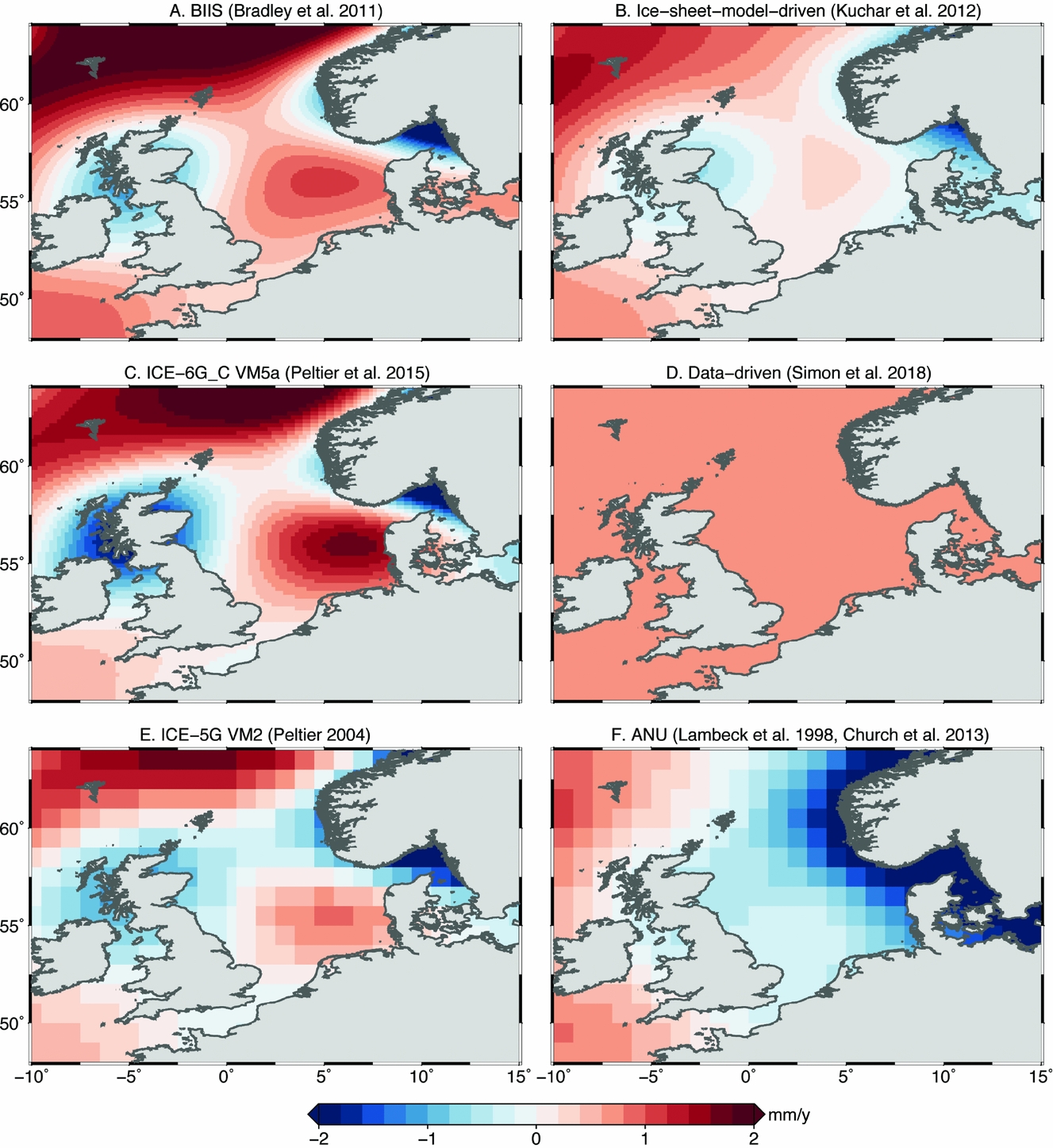
Most of the available modelling results for the North Sea are based on one-dimensional (1D) linear rheology, and results are calibrated to fit crust and mantle below the centres of uplift (i.e. Scandinavia and Scotland). In the widely used global ICE-5G(VM2) GIA model (Peltier, Reference Peltier2004), the bulk of the North Sea experiences a RSL rise of 0.1–0.5mma−1 (Fig. 6). RSL fall is modelled towards the northwest (British Isles) and northeast (Fennoscandia). Similar but slightly higher values are computed according to the most recent ICE-6G-VM5a model (Peltier et al., Reference Peltier, Argus and Drummond2015).
However, the first-order assumption of a 1D rheology may not be suitable for the North Sea area. Therefore, regional modelling studies adjust the earth rheology parameters for this specific region. For example, Bradley et al. (Reference Bradley, Milne, Shennan and Edwards2011) show an overall slightly higher RSL rate in the North Sea (Fig. 6). Recent studies show that further differences in local RSL rates can be expected when nonlinear 3D rheologies are used (Steffen & Wu, Reference Steffen and Wu2011; Van der Wal et al., Reference Van der Wal, Barnhoorn, Stocchi, Gradman, Wu, Drury and Vermeersen2013).
An alternative class of GIA solutions is represented by the so-called ‘empirical’ models, which are based on the inversion of space-geodetic data, in particular of uplift rates observed by GPS and gravity rates observed by the GRACE mission (see Appendix section ‘The satellite era’). Those models have the advantage of being able to also provide uncertainty estimates, but they are limited by the fact that available observations span only one to two decades, which makes it difficult to remove spurious signals originating from the land hydrological cycle.
High-frequency sea-level variability in the Wadden Sea
The effects of wind and pressure
Wind and surface air-pressure changes (also sometimes called the atmospheric loading effect) drive barotropic sea-level changes and cause storm surges as well as sea-level variability on monthly to decadal timescales. Because the Wadden Sea is shallow, the impact of wind climate on annual mean sea level is large. The total energy of the wind is fairly constant on an interannual timescale, but the distribution among individual sectorial directions varies greatly from year to year. For the Wadden Sea, the effects are considerable (Gerkema & Duran-Matute, Reference Gerkema and Duran-Matute2017). For example, in 1996, easterly winds contained more energy than southwesterly winds, whereas they are normally a few times weaker. This is immediately reflected in the annual mean sea level, which was anomalously low in 1996. Years with much energy from westerly winds have the opposite effect, a high annual mean sea level. As a result, annual mean sea level may vary by up to 2dm from year to year.
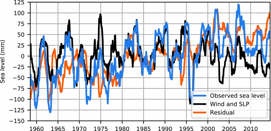
The impact of wind and pressure is location-dependent (e.g. Marcos & Tsimplis, Reference Marcos and Tsimplis2007; Dangendorf et al., Reference Dangendorf, Mudersbach, Wahl and Jensen2013; Frederikse et al., Reference Frederikse, Riva, Kleinherenbrink, Wada, Broeke and Marzeion2016a). For the Wadden Sea, a first-order estimate of the impact of wind and air pressure on sea level using linear regression with data from the JRA55 reanalysis (Kobayashi et al., Reference Kobayashi, Ota, Harada, Ebita, Moriya, Onoda and Miyaoka2015) is shown in Figure 7. The figure shows that a substantial fraction of the observed sea-level variability has its origin in wind- and air-pressure changes. Note that the local impact of wind may vary substantially along the Wadden Sea, and the impact at a specific tide gauge may thus deviate from the region-mean impact shown in the figure (Dangendorf et al., Reference Dangendorf, Calafat, Arns, Wahl, Haigh and Jensen2014a). In particular, the morphology and the direction of the coastline with respect to the dominant wind direction affect the sensitivity of sea level to the wind climate, also at an annual timescale (Gerkema & Duran-Matute, Reference Gerkema and Duran-Matute2017).
Impact of wind and surface air pressure on sea level for the Wadden Sea, estimated using a linear regression with monthly local wind and sea-level pressure (SLP) time series for each individual station, obtained from the JRA55 reanalysis (Kobayashi et al., Reference Kobayashi, Ota, Harada, Ebita, Moriya, Onoda and Miyaoka2015). Each time series has been low-pass filtered using a 12-month moving average.
A substantial part of the interannual variability in wind patterns around the North Sea is driven by the North Atlantic Oscillation (NAO). Changes in the NAO are related to the atmospheric pressure difference between the persistent high-pressure area around the Azores and the low-pressure area around Iceland.
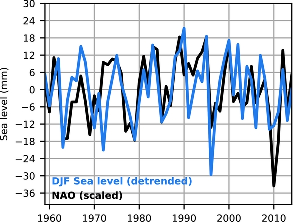
The state of the NAO is often quantified by a NAO index. The NAO affects the direction and strength of the winter-mean wind in the North Sea, with stronger westerly winds in the North Sea when the NAO index is positive, and more easterly winds during a negative phase (Hurrell et al., Reference Hurrell, Kushnir, Ottersen, Visbeck, Hurrell, Kushnir, Ottersen and Visbeck2003). The barotropic response of the North Sea results in higher winter-mean sea level during positive NAO phases along the eastern coast (Wakelin et al., Reference Wakelin, Woodworth, Flather and Williams2003). Next to a barotropic response, a small baroclinic contribution of NAO-related variability affects coastal sea level (Chen et al., Reference Chen, Dangendorf, Narayan, O'Driscoll, Tsimplis, Su and Pohlmann2014). The detrended correlation coefficient between the annual winter-mean sea level and the NAO index is 0.61 (Fig. 8).
Coherence between winter sea-level variability in the Wadden Sea and the North Atlantic Oscillation. The blue line depicts the annual winter-mean sea level (averaged over December, January, February) in the Wadden Sea (DJF Sea Level). The orange line depicts the NAO index, scaled by the ratio of the standard deviations. Both time series have been detrended.
Recent research has shown that the pressure difference between the Iberian Peninsula and Scandinavia shows a higher correlation with winter sea level in the southeastern North Sea, compared to the traditional NAO index (Dangendorf et al., Reference Dangendorf, Calafat, Arns, Wahl, Haigh and Jensen2014a). Furthermore, other atmospheric pressure patterns, including the Scandinavia Pattern and East Atlantic Pattern, also affect sea-level variability in the North Sea, and due to the interplay between these atmospheric pressure patterns, the correlation between NAO and sea level is non-stationary (Chafik et al., Reference Chafik, Nilsen and Dangendorf2017). Changes in these large-scale atmospheric pressure oscillations may result in an increase in future sea-level variability and extremes.
An indirect atmospheric effect is through freshwater discharge from rivers. De Ronde et al. (Reference De Ronde, Baart, Katsman and Vuik2014) found no significant correlation between the river outflow (for which the discharge at Lobith was taken as a proxy) and annual mean sea level at six tide gauge stations in the Netherlands. However, numerical model results and observations from local tide gauges suggest that local effects may be significant. Gerkema & Duran-Matute (Reference Gerkema and Duran-Matute2017) showed that annual mean sea level is noticeably higher (by more than 1dm) in areas adjacent to the freshwater sluices at Den Oever and Kornwerderzand.
Tides
The tide enters the North Sea from the Atlantic around the coast of Scotland and via the English Channel. Strictly speaking, tides are also generated inside the North Sea. However, the surface signature of these internal tides is small. Because of resonance characteristics, tidal amplitudes are amplified in the Wadden Sea. Changes in sea level affect tidal propagation so that tidal dynamics in the North Sea and Wadden Sea will change; in the North Sea the change in mean high water can be larger than ±10% of the imposed local SLR (Pickering et al., Reference Pickering, Horsburgh, Blundell, Hirschi, Nicholls, Verlaan and Wells2017). Assuming a constant (or: relative to SLR slow varying) bed level, sea-level rise implies a larger water depth. This decreases the impact of friction and decreases the amount of intertidal area affecting tidal asymmetry (i.e. less generation of overtides) and associated high and low water values (Friedrichs & Aubrey, Reference Friedrichs and Aubrey1988).
Empirical evidence (Louters & Gerritsen, Reference Louters and Gerritsen1994) suggests that rising sea levels affect high tides more than low tides, with implications for extremes. Morphological changes and subsidence modify the tidal characteristics as well. A final factor is an effect on the tidally generated Stokes’ drift (Van der Wegen, Reference Van der Wegen2013) enhancing mean water levels in the Wadden Sea, although this latter effect will probably be small compared to sea-level rise (SLR).
A crucial question is how the bathymetry (and in particular the intertidal area in the Wadden Sea) will react to SLR. The bathymetry may rise or erode in locally varying patterns. This depends on hydrodynamic processes (tides, wind waves, storms), as well as on sediment type, sediment supply, and sediment transport processes filling channels and building up shoals. The aforementioned tidal asymmetry plays a crucial role in tide residual sediment transport mechanisms. However, there may be an inertia in the morphodynamic system so that basin infilling (Dissanayake et al., Reference Dissanayake, Ranasinghe and Roelvink2012; Van der Wegen, Reference Van der Wegen2013; Van Maanen et al., Reference Van Maanen, Coco, Bryan and Friedrichs2013) and shoal accretion (Van der Wegen et al., Reference Van der Wegen, Jaffe, Foxgrover and Roelvink2017) lags behind anticipated SLR. Further details on the morphology of the Wadden Sea will be discussed in Wang et al. (Reference Wang, Elias, Van der Spek and Lodder2018).
Storm surges and mean sea level
Storm surges affect the sea level during and immediately after a storm, while on longer timescales they hardly leave a fingerprint on the mean sea level. For example, Gerkema & Duran-Matute (Reference Gerkema and Duran-Matute2017) considered a 20-year record of the tide gauge at Den Helder (period 1996–2015), with data at 10-min intervals. During this period, mean high tide was +59cm, mean low tide −80cm. The highest level in this record is +271cm. The cumulative effect of surges higher than or equal to a ‘low storm surge’ (mean high tide plus 100cm, i.e. higher than +159cm) was shown to contribute on average only +0.34cm to the annual mean sea level, and in none of the years more than +1.0cm. This is only a minor part of the interannual variability of mean sea level, which can be as much as a few decimetres. Although intense, the extreme events are too short-lived to leave a fingerprint on the annual mean level. Conversely, however, the results of Vousdoukas et al. (Reference Vousdoukas, Mentaschi, Voukouvalas, Verlaan and Feyen2017) suggest that changes in mean sea level can result in a change in extremes, both in terms of level and frequency.
Changes in the occurrence and intensity of storm surges due to climatological changes in the atmosphere fall outside the scope of this survey. We refer to a study by De Winter et al. (Reference De Winter, Sterl and Ruessink2013) for the North Sea, which showed on the basis of model projections that maximum wind speeds are not expected to change, or that storminess has an upward trend. On the other hand, extreme wind effects could be more directed from the west.
Regional sea-level change observations in the North Sea and the Wadden Sea
The palaeo-record
Types and qualities of palaeo-observations
The nature of palaeo-sea-level observations is predominantly sediment-geological. Certain features in the depositional architecture, sedimentological structure and fossil-bearing and pedological properties of naturally laid sediments are observed. Then, key beds deposited in an intertidal or supratidal coastal, tidal-lagoonal salt marsh, lagoon reed fringe or coastal-deltaic swamp palaeo-environment are identified. Based on properties of these beds and drawing on analogies of deposition of the same type of beds in modern environments, an ‘indicative meaning’ and associated uncertainty are assigned to the vertical distance of the bed relative to the water level at the time of deposition (e.g. Shennan et al., Reference Shennan, Long and Horton2015), usually expressed as an offset relative to mean sea level (MSL) or mean high tide water level (MHW). Using the depth of marker bed as a palaeo-sea-level observation thus requires calculating present depth ± indicative meaning offset. If MHW is used as a reference level, either a MHW reconstruction through time can be made or, if the relation between MHW and MSL is known or estimated, a MSL reconstruction can be derived as well.
When working with sets of palaeo-sea-level observations, thorough assessment of the associated vertical error is of vital importance as this makes it possible to distinguish between high-quality and medium- or low-quality data points, and to calculate the uncertainty around rates of sea-level changes (see Hijma et al. (Reference Hijma, Engelhart, Törnqvist, Horton, Hu, Hill, Shennan, Long and Horton2015) for protocols). Furthermore, the marker bed needs to be assigned an age. This can be done by sampling and dating the bed itself or by collecting dates from bracketing beds. Numeric ages (with an associated uncertainty) can be obtained from suitable material using radiometric lab techniques (e.g. on organic fossils in the beds that appear in situ). Alternatively, the numeric ages can be transferred by exploiting correlations, for instance based on contained archaeology or the presence of certain invasive biota and pollutants.
When age, elevation and indicative meaning in a sea-level reconstruction context are established (Bennema, Reference Bennema1954; Van Straaten, Reference Van Straaten1954; Jelgersma, Reference Jelgersma1961; Van de Plassche, Reference Van de Plassche1982; Denys & Baeteman, Reference Denys and Baeteman1995; Kiden, Reference Kiden1995; Shennan et al., Reference Shennan, Bradley, Milne, Brooks, Bassett and Hamilton2006; Hijma & Cohen, Reference Hijma and Cohen2010; Vis et al., Reference Vis, Cohen, Westerhoff, Veen, Hijma, van der Spek, Vos, Shennan, Long and Horton2015; Vos, Reference Vos2015), the palaeo-observation can be used as a sea-level index point. Ideally, multiple sea-level index points are available to construct past sea levels in order to have a dense enough dataset to study past fluctuations in the rate of change, and to assess spatial differences in relative sea-level change. Series of sea-level index points are typically plotted in time–depth diagrams, to reveal past rates of relative sea-level rise and compare palaeo-observations to the modern position. One analyses multiple data from a study area in stratigraphic order and considering spatial position and assesses whether the palaeo-sea-level indications replicate and if and what age–depth relations exist.
Next to sea-level index points with defined indicative meaning, it is also possible to use limiting data points to constrain past sea level. Limiting data points are obtained from indicators of which the elevational relationship to past sea level cannot be quantified, but for which it is known that they formed either above or below sea level. To be useful, the elevational range in which they formed should not be too far off past sea level. Preferably both the limiting data points and the index points are sampled from indicative beds that overlay a consolidated substrate and hence experienced little post-sedimentary subsidence due to compaction of the underlying sediments. These so-called basal points are preferred above dates from e.g. peat beds higher up in the Holocene coastal sequence, that occur intercalated with clay beds and therefore are difficult to correct for compaction-displaced positions.
In the Netherlands, basal peat is present in vast areas in the subsurface of the Holocene coastal plain, and sampling and dating it has been the focus of a great number of sea-level studies. Basal peats formed when sloping Pleistocene surfaces in the (northern) Netherlands gradually submerged due to rising groundwater levels. Because sea level continued to rise, the zone of basal peat development shifted landwards (‘transgressed’) into topographically higher areas, while the lower-lying peats were gradually covered by marine deposits (Jelgersma, Reference Jelgersma1961; Kiden et al., Reference Kiden, Makaske and van de Plassche2008).
The abundance of basal peat in the subsurface of the Netherlands gave the opportunity for an early start of Holocene sea-level reconstructions (Bennema, Reference Bennema1954; Jelgersma, Reference Jelgersma1961). For basal peat development, it is reasoned that in the temperate humid conditions of the Netherlands in the Holocene, peat formation in the coastal plain took place at or above, but never (much) below, MSL (Van de Plassche, Reference Van de Plassche1982; Roep & Beets, Reference Roep and Beets1988; Van de Plassche & Roep, Reference Van de Plassche, Roep, Scott, Pirazolli and Honig1989; Kiden, Reference Kiden1995; Kiden et al., Reference Kiden, Denys and Johnston2002, Reference Kiden, Makaske and van de Plassche2008; Hijma & Cohen, Reference Hijma and Cohen2010). At inland locations, basal peat also formed at elevations decimetres to 2m above contemporary water levels of sea and lagoons. Dated samples from such basal peats should be treated as limiting data points rather than as index points, especially where the lower part of the peat bed is dated and when the basal-peat sample comes from a coastal swamp relatively far inland (at the time of its deposition), which is controlled by local groundwater conditions. As part of the screening of larger sets of data points (e.g. Fig. 9), it is important to separate localities where peat formation occurred in response to local groundwater conditions from sites where rising sea levels triggered peat formation (Van de Plassche, Reference Van de Plassche1982; Cohen, Reference Cohen, Giosan and Bhattacharaya2005). Careful screening and analysis of each individual basal-peat point is needed to arrive at robust insights on the difference in relative sea-level rise from place to place and between regions.
Lumped overview of palaeo-observations on sea level in and around the Wadden Sea in the Southern North Sea. Each dot holds a geological sample location from which depth and age of former sea-level positions could be estimated. Accuracy and indicative meaning of such index points differ greatly between samples and suites-of-samples. The data overview figure is compiled from archived materials in institutional databases of TNO Geological Survey of the Netherlands, Utrecht University and Rijksuniversiteit Groningen, as collected by various past (Berendsen, De Groot, Jelgersma, De Jong, Van de Plassche, Törnqvist, Zagwijn and others) and currently active workers (Busschers, Cleveringa, Cohen, Hijma, Kiden, Koster, Makaske, Meijles, Peeters, Pierik, Vos), including recently acquired samples. Outside the Dutch sectors, the figure draws upon overviews from the UK (Shennan et al., Reference Shennan, Lambeck, Horton, Innes, Lloyd, McArthur and Rutherford2000), Belgium (Denys & Baeteman, Reference Denys and Baeteman1995) and Germany (Behre, Reference Behre2007). Each sample should be screened in detail according to the protocol of Hijma et al. (Reference Hijma, Engelhart, Törnqvist, Horton, Hu, Hill, Shennan, Long and Horton2015) to be included in a palaeo-sea-level database.
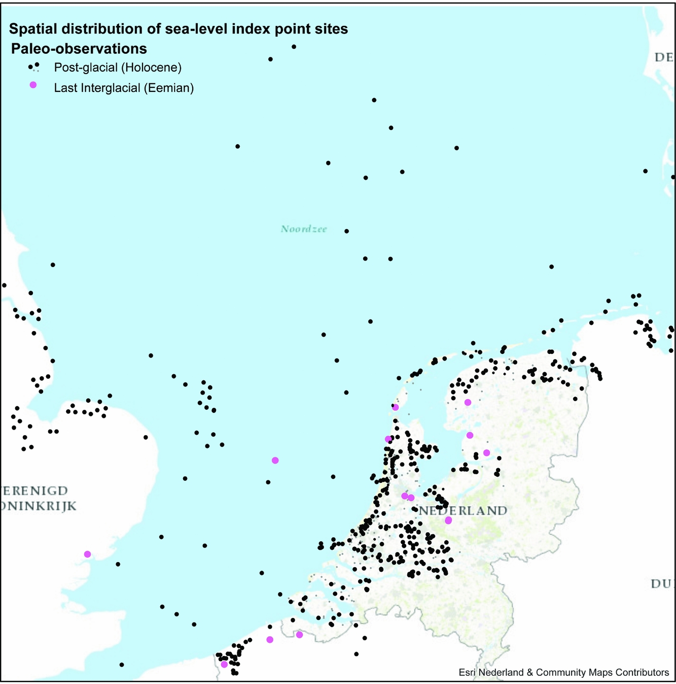
Figure 9 shows the spread of index points available for the Wadden Sea and surroundings for the Last Interglacial and Holocene periods. The figure combines multiple types of palaeo-observations of vertical position and age. The figure gives an impression of the density of sea-level rise constraining observations as currently available, and the differences in density between different offshore and onshore sectors of the North Sea and the Dutch coastal plain (with the Wadden Sea in the middle). The figure plots the available acclaimed raw index-point data after a first round of screening.
Further scrutiny of data points is needed before they can be used to iterate high-quality sea-level rise reconstructions for use at regional to local scale. Specific attention needs to be paid to differences in the accuracy of sampling and elevation control as standards and level of attention to certain aspects have changed over the years. In addition, care has to be taken as to the fact that sedimentary environments providing index points by their nature have different associated accuracy. It should be noticed that many of the Holocene RSL palaeo-observations originate as by-products of general-purpose geological–geomorphological mapping and archaeological site surveys and excavations. For the Wadden Sea region, with focus on the Holocene, several studies have been exemplary in producing sets of sea-level index points (Roeleveld, Reference Roeleveld1974; Griede, Reference Griede1978; Oost, Reference Oost1995; Van der Spek, Reference Van der Spek1996; Vos, Reference Vos2015). The comprehensive studies of Roeleveld (Reference Roeleveld1974) and Griede (Reference Griede1978) and more recently Vos (Reference Vos2015) focused on coastal landscape evolution rather than on sea-level reconstruction. Studies by Oost (Reference Oost1995) and Van der Spek (Reference Van der Spek1996) focus on long-term Wadden Sea sedimentation and morphodynamics, rather than on sea-level reconstruction.
A last reason for careful selection of data points (independent of diversity in research history and sampling biases) is that spatially varying tidal ranges, river discharge and groundwater-flow regimes have influenced the elevation at which basal peats grow and at which regular flood sedimentation occurs (Van de Plassche, Reference Van de Plassche1982; Berendsen et al., Reference Berendsen, Makaske, Van de Plassche, Van Ree, Das, Van Dongen, Ploumen and Schoenmakers2007; Kiden et al., Reference Kiden, Makaske and van de Plassche2008; Hijma & Cohen, Reference Hijma and Cohen2010; Baeteman et al., Reference Baeteman, Waller and Kiden2011; Vis et al., Reference Vis, Cohen, Westerhoff, Veen, Hijma, van der Spek, Vos, Shennan, Long and Horton2015). A priori (i.e. at the moment of deciding to take a sample in the field and processing it in the lab), it is difficult to estimate for individual samples to what degree the sample will have been subject to the above effects and what the indicative meaning and quality of the index point is. As it happens, at some places basal peats established at positions over 1m above contemporary sea level, where in other situations it formed just 10–20cm above it. Likewise, supratidal salt marsh in some areas along the Wadden Sea established above the high water line, c.1m above MSL, where in other places it does so at 1.5 m. This means that these effects can only be assessed a posteriori, and one can start this process only once a certain number of data points from a series of locations within a segment of coastal plain have been collected and when insight on palaeo-tide levels is present. For each region where a sea-level curve is wanted, the most seaward, youngest–deepest sampled basal peats should be searched for, as they constrain sea-level reconstructions best (Cohen, Reference Cohen, Giosan and Bhattacharaya2005; Hijma & Cohen, Reference Hijma and Cohen2010; Vis et al., Reference Vis, Cohen, Westerhoff, Veen, Hijma, van der Spek, Vos, Shennan, Long and Horton2015). The next section includes a basal-peat index-point screening for the northern Netherlands, based on Kiden & Vos (Reference Kiden and Vos2012) and Meijles et al. (accepted).
For the Holocene, the types of palaeo-observations included in Figure 9 mainly cover sets of 14C-dates from basal peats sampled along the flanks and tops of buried Pleistocene topography, encountered underneath younger shallow marine and lagoonal deposits (at depth in the coastal plains of Groningen, Friesland, Holland, Zeeland, Belgium; distribution inland follows buried valleys). Depending on the geographical position and setting, these basal peats date to between 8000 and 4000 years ago. In offshore areas, submerged basal peats are also encountered, dated between 10,000 and 8000 years before present, when the Wadden Sea and the Netherlands were still terrestrial environments (e.g. Behre & Mencke, Reference Behre and Mencke1969; Jelgersma, Reference Jelgersma1979; Ludwig et al., Reference Ludwig, Müller and Streif1981; Behre et al., Reference Behre, Dörjes and Irion1984; Shennan et al., Reference Shennan, Lambeck, Horton, Innes, Lloyd, McArthur and Rutherford2000; Alappat et al., Reference Alappat, Vink, Tsukamoto and Frechen2010; Wolters et al., Reference Wolters, Zeiler and Bungenstock2010). The environments of the Wadden Sea and its barrier system of tidal inlets and the Wadden Islands established 8500–5000 years before present (Oost, Reference Oost1995; Van der Spek, Reference Van der Spek1996), as did those of the rest of the southern North Sea coastal-deltaic plain (e.g. Hageman, Reference Hageman1969; Kiden, Reference Kiden1995; Beets & Van der Spek, Reference Beets and van der Spek2000; Vos, Reference Vos2015).
The onshore basal peat data cover the Middle Holocene (8000–4000 years before present) relatively well, with dense sampling in multiple subenvironments in the Netherlands, providing fair insight into relative sea-level rise and regional and environmental differences. Sampled basal peats from the Early Holocene (11,000–8000 years before present) from offshore areas are much fewer in number, as these areas are more difficult to survey and sample. For the Late Holocene (the last 4000 years), basal peats are hardly available in the Netherlands, because in great parts of the coastal plain the landscape changed dramatically as people began to use it with increasing intensity. Organic landscape components have decomposed: due to agriculture and drainage water, few survived as preserved deposits. In the absence of basal peat, a variety of other types of observational evidence is used as palaeo-sea-level indicators in the Late Holocene. This includes observations obtained from Late Holocene ‘wadden’ and ‘salt marsh’ depositional environments (inland within the coastal plain), as well as from beach-barrier and coastal dune foot environments (truly coastal).
The Late Holocene of the coastal Netherlands is known for its many neighbouring ingressive tidal systems, each fast evolving (Vos & Knol, Reference Vos and Knol2015; De Haas et al., Reference De Haas, Pierik, van der Spek, Cohen, van Maanen and Kleinhans2017; Pierik et al., Reference Pierik, Cohen, Vos, van der Spek and Stouthamer2017). Along the inland parts of the coastal plain (including former salt marsh areas in Friesland and Groningen: dwelling mount areas, embanked in the last 1000 years), the currently available data for the last 3000 years are insufficiently spatially dense to resolve sea-level change signals from the local tidal changes resulting from opening and/or silting up of tidal channels. Considerably denser sampling of index points would be needed in combination with palaeo-tidal numeric modelling, to disentangle sea-level from tidal change signals. A further approach that could be beneficial to the quality of the palaeo-observational data would be to make use of salt-marsh diatom microfossil records. This method was applied with reasonable success on the English North Sea coast. A few studies exist that used alternative types of sedimentary sea-level indicators in the Holland beach-barrier and coastal-dune complex (e.g. Roep, Reference Roep and van de Plassche1986; Van de Plassche & Roep, Reference Van de Plassche, Roep, Scott, Pirazolli and Honig1989). De Groot et al. (Reference De Groot, Westerhoff and Bosch1996) explored the records for the Wadden Islands, as discussed below.
Vertical spread of palaeo-observations, general sea-level curves
All sea-level index points are relative sea-level index points (RSL index points). In the setting of the Netherlands, this means that they have subsided since deposition, and have done so at variable rates over space and time. The age–depth distributions of palaeo-observations contain signals of relative sea-level rise in the Holocene and Eemian time intervals (Fig. 10).
The Netherlands’ records of relative sea-level rise for the Holocene and the Eemian (Cohen et al., Reference Cohen, Peeters, Sier, Hijma and Busschers2016). The left panel shows the Holocene response of sea level to the melt of the large ice sheets (SIS = Scandinavian Ice Sheet; LIS = Laurentide Ice Sheet and AIS = Antarctic Ice Sheet). The right panel shows the position of sea-level indicators and sea-level reconstruction for the Netherlands during the Eemian, supplementing data points from Zagwijn (Reference Zagwijn1983, Reference Zagwijn1986). Global sea level is estimated to have been 6–9m higher than the present level (Dutton et al., Reference Dutton, Carlson, Long, Milne, Clark, DeConto, Horton, Rahmstorf and Raymo2015), but due to subsidence in the last 120,000 years, the sea-level indicators presently lie at −8m and deeper.
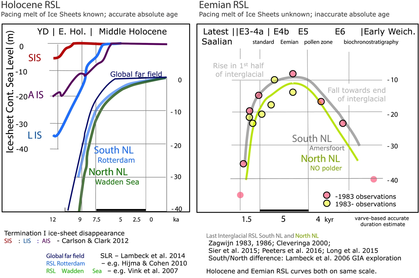
The palaeo-observations and sea-level curves for the western and northern Netherlands and northern Germany plot at deeper positions than global far-field datasets for the same periods. This subscribes to the notion of near-field GIA subsidence affecting the study area (introduced in sections above). Within the Netherlands, the Wadden Sea and surroundings show the greatest rates of relative sea-level rise, at least in the first half of the Holocene. Curves for the central and southern parts of the Netherlands plot higher than those for the northern Netherlands. This means that coastal deposits from which the observations have been derived have differentially subsided since their deposition: by a greater amount in the north, relative to the south (Kooi et al., Reference Kooi, Johnston, Lambeck, Smither and Molendijk1998; Kiden et al., Reference Kiden, Denys and Johnston2002; Vink et al., Reference Vink, Steffen, Reinhardt and Kaufmann2007; Koster et al., Reference Koster, Stafleu and Cohen2017).
Subsidence since deposition is particularly evident for the RSL index points of the Last Interglacial (Fig. 10). The Eemian sea-level records in the Netherlands are more patchily preserved and are less easily dated, but they are always buried at greater depth than their Holocene counterparts. This is explained by their burial depth, the erosive attacks on the Eemian record during sea-level fall and the return to cold climate conditions in the last glacial.
The northern Netherlands and the Wadden Sea historically have a lower intensity of shallow geological surveying compared to heavily urbanised and industrialised parts of the coastal plain of the western Netherlands (notably the Rotterdam area). In addition, geological differences between the two areas make the areas in the north less suitable for collecting palaeo-sea-level observations than the western Netherlands. Below the northern Netherlands’ coastal plain, patches of basal peat have been preserved in lows in the transgressed surface, such as former valley floors, in the same way as in the western Netherlands. What is lacking, however, are local positive relief features of sufficient height, where one can collect a series of index points spanning a few metres vertically. In the Rhine delta and Flevo lagoon, inherited inland dune topography preservation is much more complete, encapsulated in mud and organics, providing superb sea-level sampling localities (e.g. Van de Plassche, Reference Van de Plassche1995; Makaske et al., Reference Makaske, van Smeerdijk, Peeters, Mulder and Spek2003; Van de Plassche et al., Reference Van de Plassche, Bohncke, Makaske and van der Plicht2005). In the north, such sites are rare and have yet to be sampled. Hence, to use basal peat from shallow depth intervals as sea-level indicators one has to rely on inland sampling locations, which are more likely to yield data points of the limiting type rather than true sea-level indicators.
The above reasons explain why, until recently, no Holocene sea-level reconstruction was available for the northern Netherlands and the Dutch Wadden Sea area. Based on a critical evaluation of the limited available data, Van de Plassche (Reference Van de Plassche1982) hypothesised that the sea-level reconstruction for the western Netherlands was also representative for sea-level rise in the north. On the other hand, more recent research, combining sea-level data with GIA model results, suggests stronger glacio-hydro-isostatic subsidence and greater rates of relative sea-level rise in the northern Netherlands than in the western Netherlands (Kiden et al., Reference Kiden, Denys and Johnston2002; Vink et al., Reference Vink, Steffen, Reinhardt and Kaufmann2007). Kiden & Vos (Reference Kiden and Vos2012) and more recently Meijles et al. (accepted) investigate this discrepancy by means of new compilations of palaeo-sea-level data to more accurately reconstruct Holocene relative sea-level rise in the Wadden Sea and the adjacent coastal plain.
Selection and analysis of palaeo-observation data
For the Wadden Sea region, an intensive data search for dated peat samples, from literature and from archives of the Geological Survey of the Netherlands and the Centre for Isotope Research, yielded a dataset of more than 250 samples. From this, an initial set of 51 possibly suitable basal-peat dates was selected. Plotting the 51 radiocarbon samples in a time–depth diagram resulted in a distribution of index points with a sharp lower boundary and a diffuse upper limit (Fig. 11). On the basis of the diagram, 26 index points were considered suitable for sea-level reconstruction (screening details in Meijles et al., accepted).
Time–depth diagram of the 51 originally selected radiocarbon-dated basal peat samples in the Northern Netherlands coastal area. The age (‘cal. ka BP’) is in years before present, the altitude in metres below NAP (Normaal Amsterdams Peil or Dutch Ordnance Level), which is within 0.1m of present-day MSL. Red dots indicate samples from peat beds that were formed above contemporary sea level and thus cannot be used as sea-level indicators. The 26 index points in the lowest time–depth position (black dots) are interpreted to track sea level and are used for the reconstruction of the sea-level curve and error band. Vertical error bars contain primarily errors in altitude determination but no estimate of the indicative meaning of the index points. See Meijles et al. (accepted) for further details on data selection, evaluation and error term treatment.
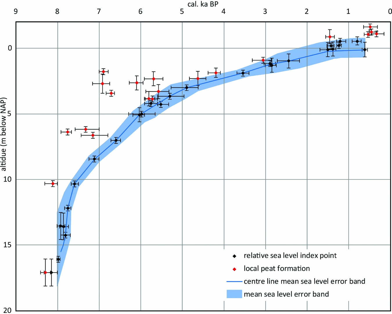
The selected data and the sea-level curve derived from them (Fig. 11) show a sharp rise 8000–7500 years ago with an average rate of 10mma−1. The horizontal and vertical uncertainty in this section is high. The rate decreases to c.2.5mma−1 between 7500 and 4000 years ago with a total rise of nearly 7.5m with a temporally variable vertical error envelope. After 4000 to c.1500 years ago the rate of sea-level rise reduced to a relatively stable 0.9mma−1. In the most recent section of the curve (1500–600 years ago), the average rate of sea-level rise is in the order of 0.2mma−1, but since the vertical uncertainties are high, this merely indicates that the rate of RSLR was low.
The curve for the Wadden Sea has a considerably lower time–depth position than those for Belgium (Denys & Baeteman, Reference Denys and Baeteman1995) and Zeeland (southwestern Netherlands; Kiden, Reference Kiden1995; Vink et al., Reference Vink, Steffen, Reinhardt and Kaufmann2007), especially in the older part (Fig. 12). The vertical difference decreases from 4–6m c.8000 years ago to 2m c.6000 years ago. Note that the error envelope centre lines for Zeeland and Belgium are completely outside the error envelope of the Wadden Sea curve. After 5000–4000 years before present the respective curve error envelopes slowly converge and in the last 3000 years they merge.
The relative mean sea-level reconstruction for the Wadden Sea compared to relative sea-level curves for neighbouring coastal areas (Meijles et al., accepted).
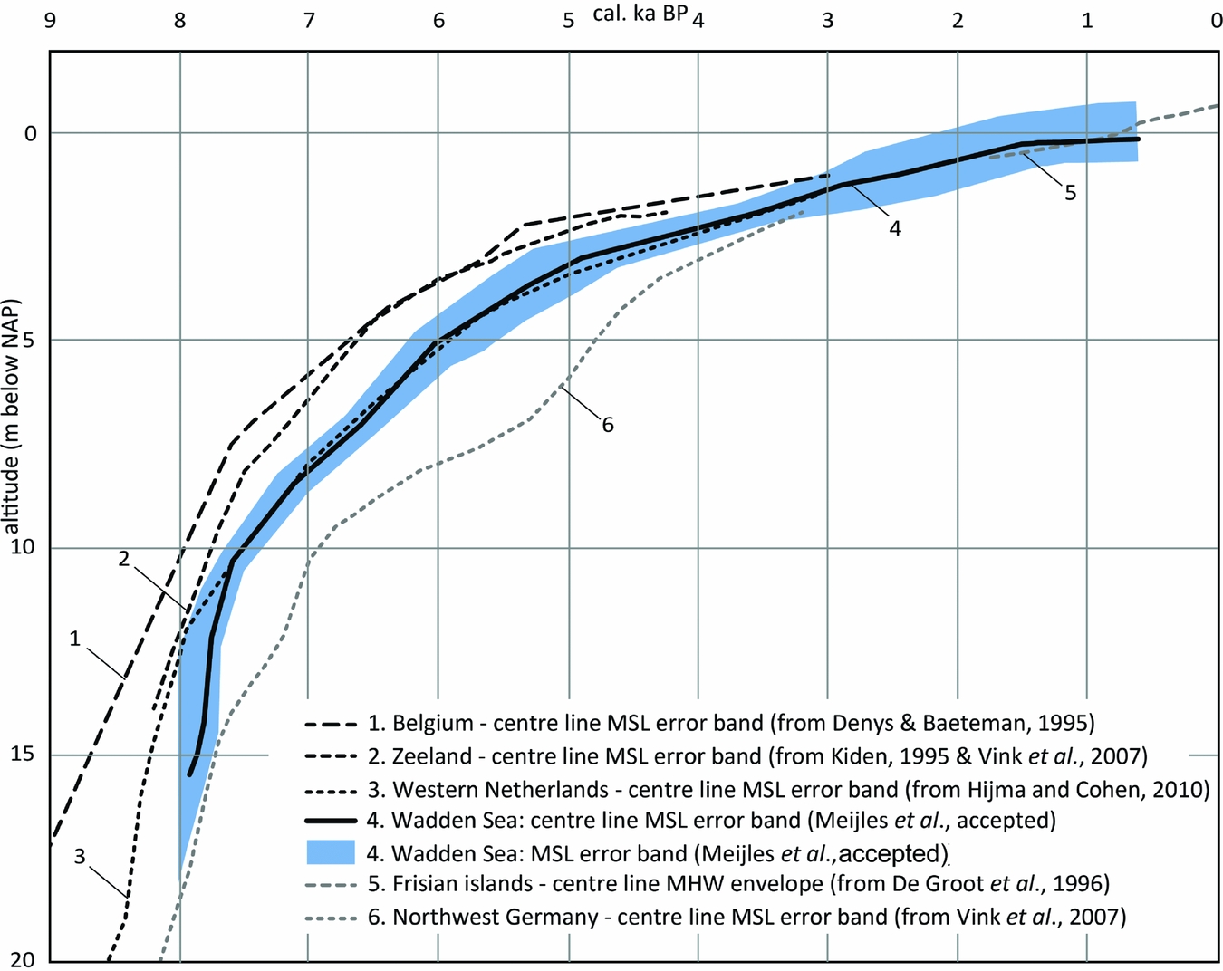
In its older part, the Wadden Sea curve (Fig. 13) also plots lower than recent sea-level reconstructions for the western Netherlands for that period (Fig. 12; Hijma & Cohen, Reference Hijma and Cohen2010; Van de Plassche et al., Reference Van de Plassche, Makaske, Hoek, Konert and van der Plicht2010). The difference in depth positions of the older parts of the curves is evidence for differential subsidence of the northern Netherlands relative to the southwestern Netherlands and Belgium, and to a lesser extent to the western Netherlands. The rapidity of the drop appears to indicate a larger GIA subsidence towards the north, with the difference in rates decreasing into younger time. The observed difference in subsidence is also greater than that expected from tectonic land movement, pointing to GIA-induced subsidence. This is consistent with the notion of Kiden et al. (Reference Kiden, Denys and Johnston2002) that GIA modelling predicts sea-level index points in the north to be encountered at greater depth, at least in the older part of the Holocene. For the period after c.7500 before present, however, no significant difference remains between the Wadden Sea sea-level reconstructions and those for the western Netherlands. The latter is in disagreement with GIA model predictions (in their current iterations) and reproduces the notion of Van de Plassche (Reference Van de Plassche1982). This is further explored in the next section.
The relative mean sea-level reconstruction for the Wadden Sea compared to the Glacial Isostatic Adjustment (GIA) and tectonics-corrected reference relative MSL error band for Belgium (Denys & Baeteman, Reference Denys and Baeteman1995); for further explanation see Meijles et al. (accepted).

Sea-level records of the Wadden Sea for the last 2500 years
To assess future sea-level rise, knowledge of sea-level change in the recent past is of prime importance. However, similar to other basal-peat-based sea-level studies in the Netherlands (see above), the sea-level reconstruction in Figures 11–13 does not extend to the present day, as the youngest index point has an age of c.600 years before present. Moreover, for the last 3000–2000 years the uncertainty range is relatively large.
In Figure 11, the index points for the period 1800–1000 years ago are from local peat layers sampled in lows in the coastal dune terrains on the Wadden Islands. These peat layers are known to have formed in settings where local freshwater lenses maintain groundwater-table positions that are decimetres to metres above contemporary mean sea level, as observed on the Wadden Islands today (Grootjans et al., Reference Grootjans, Sival and Stuyfzand1996; Röper et al., Reference Röper, Kröger, Meyer, Sültenfuss, Greskowiak and Massmann2012). Such locally raised coastal-dune groundwater tables can be explained by density differences between salt- and fresh water (Drabbe & Badon Ghijben, Reference Drabbe and Badon Ghijben1889; Herzberg, Reference Herzberg1901).
On the Wadden Isles, raised groundwater levels of over 2m above MSL have been measured on Spiekeroog in Germany (Tronicke et al., Reference Tronicke, Blindow, Groß and Lange1999) and to 3.5m above MSL locally on Schiermonnikoog (Grootjans et al., Reference Grootjans, Sival and Stuyfzand1996). Peat samples on the Wadden Islands are indicative of higher groundwater levels due to the freshwater lens effect and as such can only be used as upper limit indicators for sea level. It is thus presumed that the actual sea level during the last 1800 years will have been slightly (c.1 m) below the index points shown in Figure 11 from that period.
Using sea-level indicators from settings other than peat beds (e.g. diatom assemblages in salt marsh muds) would make it possible to more narrowly constrain sea levels in the last 2000 years in the Wadden Islands, but such methods at present have not been applied in the Netherlands.
Given these uncertainties in the sea-level reconstruction of Meijles et al. (accepted) for the last 2000 years, it is interesting to compare that part of the Wadden Sea curve with the MHW upper limit curve for that same period by De Groot et al. (Reference De Groot, Westerhoff and Bosch1996). Their comprehensive study on the Frisian Wadden Islands is one of the few such studies available for this time period in the Netherlands, and hence important in bridging the gap between the Holocene geological record and the historical modern instrumental record.
The sea-level reconstruction by De Groot et al. (Reference De Groot, Westerhoff and Bosch1996) is featured in Figure 14. It is based on radiocarbon-dated coastal sedimentary sequences and associated palaeoecological evidence retrieved from cored boreholes and excavations on the Frisian Wadden Islands of Texel, Vlieland, Terschelling, Ameland and Schiermonnikoog. The fieldwork did not yield data on tidal levels other than MHW, and no estimate of MSL was given. To do so, information on palaeo-tides and a sound understanding of the palaeogeographical situation for the relevant time period are necessary. Another issue with the De Groot et al. dataset is that datable organic material was mostly found at a significantly higher level than the sedimentological MHW indications themselves. This means that the ages attached to the index point are (slightly) younger than the corresponding MHW heights. One could thus shift the curves in the figure to the left and raise reconstructed sea levels to a higher position earlier in time (actual MHW was higher). Doing so lowers the rate of MHW and/or sea-level rise deduced for the last 1000–500 years.
Reconstruction by De Groot et al. of the MHW trend over the last 2000 years on the Frisian Islands, based on sedimentological and palaeoecological observations and criteria (reproduced from De Groot et al. (Reference De Groot, Westerhoff and Bosch1996), timescale in uncalibrated radiocarbon years before present). MSL indicators were not found in the studied sediments so no reconstruction could be made of the MSL trend. Under the (untested) assumption that palaeo-tidal range has remained unchanged over the last 2000 years, MSL may have been 0.7–1.25m lower than the MHW reconstruction shown here, as present-day tidal range in the Dutch Wadden Sea is between 1.4 and 2.5m (Oost et al., Reference Oost, Hoekstra, Wiersma, Flemming, Lammerts, Pejrup, Hofstede, van der Valk, Kiden, Bartholdy and van der Berg2012).

A centre line through the error envelope of De Groot et al. (Reference De Groot, Westerhoff and Bosch1996), after calibrating the 14C ages over the last 1800 years, gives an average rate of rise of MHW of c.0.7mma−1. Data collected from below the soles of terps on the Frisian mainland (Vis et al., Reference Vis, Cohen, Westerhoff, Veen, Hijma, van der Spek, Vos, Shennan, Long and Horton2015; Vos, Reference Vos2015) support such a rate to apply to the first millennium BC. This suggests that the Wadden Isles and Frisian mainland data capture the same gross regional trend, but this should not be seen as a proof that relative sea-level rise was spatially uniform and/or temporally semi-linear over shorter time periods. As noted above, actual MHW rise is likely to have been lower than this. The associated error bands are large, however, and allow deducing rates of MHW rise of double the average rate, a near-zero rate or for one showing fluctuations. De Groot et al. (Reference De Groot, Westerhoff and Bosch1996), for example, note a possible acceleration of MHW rise c.850 years ago (c.800 14C yr), from c.0.6mma−1 before to 0.9mma−1 after that date. The authors were unable to determine whether this is related to short-term accelerated sea-level rise, or to factors such as changes in storm frequency and amplitude or embankment of the tidal marsh land on the Friesland mainland (dike construction). However, considering the large uncertainty around their sea-level data (including the calibration of 14C dates in the particular time interval), the apparent acceleration may be insignificant.
Despite its limitations towards the recent past as noted above, the study of Meijles et al. (accepted) yields much lower rates of MSL rise over a comparable period. Using the centre line of the error envelope of Meijles et al.’s analysis (Figs 11 and 12), an average MSL rise between 0.4 and 0.5mma−1 from c.3000 years ago to the present can be calculated, decreasing to not more than c.0.2mma−1 over the last 600 years (extrapolated to 0m NAP at present). The reasons for the discrepancy between the MHW results of De Groot et al. (Reference De Groot, Westerhoff and Bosch1996) and Vos (Reference Vos2015), and the coastal-groundwater MSL results of Meijles et al. (accepted) concerning sea-level rise in the last 3000–2000 years remain to be investigated.
Possible explanations for differences in rates and observed vertical offsets between different types of observational data – if not explained as resulting from uncertainty, noise and error in the observations – would be (i) short-term accelerations and decelerations occurring in the rate of MSL rise; (2) spatio-temporal changes in tidal amplitudes in the Wadden Sea independent of MSL variations; (3) unaccounted spatial differences in land subsidence between the sites. Considering that the error envelope of the MSL curve is more than 1m wide, it is currently not possible to robustly identify fluctuations in the rate of relative SLR in the last 2000 years, with the exception of the tide-gauge covered last centuries. What can be said is that in general the rates were low (lower than the observations and predictions of ongoing relative sea-level rise). It can be assumed that in the past fluctuations occurred in part as a response to ocean sterics (e.g. Kopp et al., Reference Kopp, Horton, Kemp and Tebaldi2015, Reference Kopp, Kemp, Bittermann, Horton, Donnelly, Gehrels, Hay, Mitrovica, Morrow and Rahmstorf2016), but equally due to the three more local effects mentioned above. These undulations must have stayed within the bandwidth indicated by the observational data figures.
The Wadden Sea is no exception
Global insights and rules of thumb regarding the availability of records and the opportunity to collect palaeo-observations apply to the Wadden Sea and the Netherlands as well. Its lowland coastal geological setting relates strongly to the global sea-level history of the last and penultimate cycles. It was only at the end of Glacial Termination I, c.8000 years ago, when postglacial sea-level had risen to levels 25–15 m below present, that the shallow North Sea floor began to drown and that chains of embryonic precursors of the coastal barriers and Wadden Islands began to establish at more or less the present coastline position. In other words: sea-level rise records of the last c.8000 years in the Wadden Sea and the Netherlands are preserved inland below the coastal plain and Wadden Sea, at depths shallower than c.25 m below present MSL, where they are not eroded by younger channel scour or human activities.
Records from transgressive stages prior to 8000 years are offshore, at shallow depth, just below the morphologically active seabed. This contrast in place, position, accessibility and degree of preservation between Middle–Late Holocene and Late Glacial – Early Holocene records is shared by the Wadden Sea and the North Sea with shelf-sea, barrier–lagoon, and deltaic coastal plain complexes around the world. This means that relative sea-level records from the last 6000 years, from circumstances of ‘a high stand’ with only modest relative sea-level change, tend to have been collected from more inland positions with slightly different subsidence and mean coastal water level properties than sites targeting the period 9000–6000 years ago, with some interpretation and data usage caveats.
Once a first Wadden Sea had formed, apart from sea-level rise, several other processes played their role in the further evolution of the Wadden Sea. Sediment from the hinterland by the rivers Rhine, Vecht, Ems and Weser/Elbe had been delivered to the North Sea floor in the Last Glacial and before, and thus was abundantly available for recirculation from the moment the North Sea transgressed the region. Then, beginning c.9000 years ago, tidal and wave-driven currents started shifting these sandy sediments. By 8000–7000 years ago, this resulted in the first barrier islands at positions in the immediate offshore of the present system (Jelgersma, Reference Jelgersma1979). Then, coeval with barrier development and depending on distance to main sediment feeds to the coastal plain, the tendency of underfilled tidal systems behind the barriers to trap large volumes of sediments in next millennia came into play (Beets & Van der Spek, Reference Beets and van der Spek2000; Oost et al., Reference Oost, Hoekstra, Wiersma, Flemming, Lammerts, Pejrup, Hofstede, van der Valk, Kiden, Bartholdy and van der Berg2012; De Haas et al., Reference De Haas, Pierik, van der Spek, Cohen, van Maanen and Kleinhans2017). By 6000–5000 years ago this had culminated in partially to fully filled tidal basins (switching from ‘transgressive’ to ‘high stand’ system modes). Then, again coeval with barrier formation and back-barrier tidal basin filling processes, the last process to consider is the tendency of marsh and swamp vegetation to create peaty substrates in the most inland parts of the coastal plain, over the pre-transgression substrate (basal peat references earlier in this section) as well as on top of tidal deposits in silted-up basins (Beets & Van der Spek, Reference Beets and van der Spek2000; Oost et al., Reference Oost, Hoekstra, Wiersma, Flemming, Lammerts, Pejrup, Hofstede, van der Valk, Kiden, Bartholdy and van der Berg2012; Vos, Reference Vos2015; Pierik et al., Reference Pierik, Cohen, Vos, van der Spek and Stouthamer2017). Altogether this has allowed for a lot of sediment accommodation in back-barrier space. In the Zeeland and Holland sectors, that accommodation left fewer back-barrier waters open, than in the Wadden Sea sectors.
The back-barrier tidal waters and coastal plain deposits in the inland direction onlap a substrate with a morphology owing to glaciation by the edge of the Scandinavian Ice Sheet c.150,000 years ago and river valley activity since then (Busschers et al., Reference Busschers, Kasse, van Balen, Vandenberghe, Cohen, Weerts, Wallinga, Johns, Cleveringa and Bunnik2007, Reference Busschers, van Balen, Cohen, Kasse, Weerts, Wallinga and Bunnik2008; Hijma et al., Reference Hijma, Cohen, Roebroeks, Westerhoff and Busschers2012; Peeters et al., Reference Peeters, Busschers, Stouthamer, Bosch, van den Berg, Wallinga, Versendaal, Bunnik and Middelkoop2016), with intercalated sedimentary sea-level records from the Last Interglacial (Zagwijn, Reference Zagwijn1983; Kiden et al., Reference Kiden, Denys and Johnston2002, Long et al., Reference Long, Barlow, Busschers, Cohen, Gehrels and Wake2015), preserved at nowadays subsided positions. In global data overviews, this lists the Wadden Sea and the Netherlands palaeo-observations, with many other sites along the European, US and Caribbean Atlantic coasts, in the group of so-called ‘Near Field’ sea-level sites. That classification implies that the palaeo-observational vertical positions are affected by GIA and gravitational effects of waxing and waning ice sheet masses, and for that reason deviate from ‘eustatic’ signals and typical vertical positions shown by sites in Far Field regions (coasts in and around the Indian Ocean and Pacific Ocean). Despite this difference with far-field sites, the Wadden Sea and the Netherlands share their coastal plain age and stratigraphy of transgressive drowning units below back-barrier fill units with basically every other barrier–lagoon, delta and estuarine system around the world (e.g. Hori & Saito, Reference Hori and Saito2007; Tamura et al., Reference Tamura, Saito, Sieng, Ben, Kong, Sim, Choup and Akiba2009; Hijma & Cohen, Reference Hijma and Cohen2011; Wang et al., Reference Wang, Zhan, Long, Saito, Gao, Wu, Li and Zhao2012; Amorosi et al., Reference Amorosi, Bruno, Cleveland, Morelli and Hong2017; Pennington et al., Reference Pennington, Sturt, Wilson, Rowland and Brown2017).
The tide-gauge record
Decadal sea-level variability and multi-decadal trends in the Wadden Sea
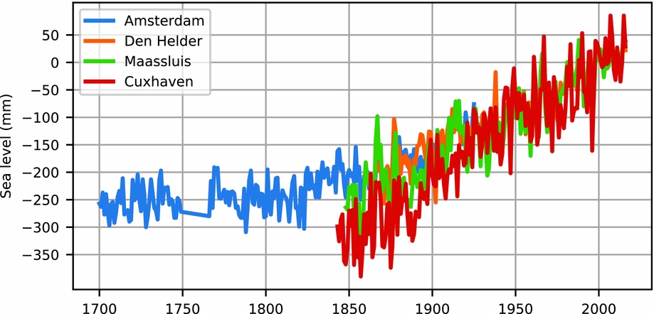
Sea level in the North Sea has been recorded by the Amsterdam tide gauge since 1700. Multiple high-quality records are available since the mid-19th century (Fig. 15). All tide gauge records, corrected for vertical land motion, show a rise in sea level in the 20th-century, although the Cuxhaven record differs from the other records. The Amsterdam record suggests that sea-level rise commenced in the second half of the 19th century. The large interannual variability, present in all records, hinders the detection of a present-day acceleration in sea level at local scales.
Annual sea level from four long-term tide gauge records in the southwestern North Sea. The common mean of the Maassluis, Den Helder and Cuxhaven stations over the last 25 years has been removed. The common mean over the overlapping period between Amsterdam and Den Helder has also been removed. The data were obtained from the Permanent Service for Mean Sea Level (PSMSL, Holgate et al., Reference Holgate, Matthews, Woodworth, Rickards, Tamisiea, Bradshaw, Foden, Gordon, Jevrejeva and Pugh2012).
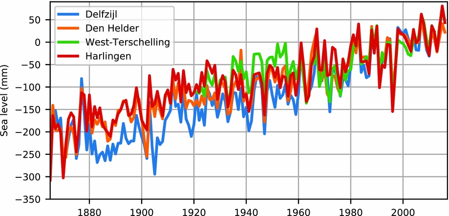
Since 1865, multiple tide-gauge records for the Wadden Sea are available (Fig. 16). They mostly show a common trend and variability signal, although the Delfzijl record shows a substantial deviation at the beginning of the 20th century. For all stations, the sea-level trend is positive and significant (Table 2), although significant differences between nearby stations exist. The acceleration is not significant at the 95% confidence level for any of the stations.
Annual sea level from four long-term tide-gauge records in the Wadden Sea. The common mean of all signals over the last 25 years has been removed. Note that Den Helder is present both in this and the previous figure.
Trends in North Sea and Wadden Sea tide gauge records (1890–2016). Trends computed after the nodal tide has been filtered out (Baart et al., Reference Baart, van Gelder, de Ronde, van Koningsveld and Wouters2012). Sea-level monitor (Version v2017.04). Zenodo. https://doi.org/10.5281/zenodo.1065964.
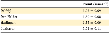
It is generally difficult to explain the origins of differences between individual tide gauges, and therefore a possible method to assess regional sea-level changes is to merge multiple records from nearby tide gauges into a regional average. Here, we merge stations from the Wadden Sea and the Dutch North Sea coast into region-mean records using the ‘virtual station’ method (Jevrejeva et al., Reference Jevrejeva, Moore, Grinsted, Matthews and Spada2014; Dangendorf et al., Reference Dangendorf, Marcos, Wöppelmann, Conrad, Frederikse and Riva2017, Frederikse et al., Reference Frederikse, Jevrejeva, Riva and Dangendorf2018). This can be used to obtain an estimate of decadal sea-level variability and multi-decadal trends in the Wadden Sea over the past 50 years, and to assess whether these quantities differ from those in the Dutch North Sea. High-frequency data at 12 Wadden Sea and 13 Dutch North Sea tide gauges (Fig. 17) obtained from the Rijkswaterstaat data portal (live.waterbase.nl) is averaged to compute monthly means. Not all stations have data over the entire analysis period. We assess the period 1958 to 2014, because over this period, estimates of ice-mass loss, density changes and land-water storage are available. These will be used to assess the origins of the observed trends and variability. In the virtual-station method, the two closest stations are merged into a new virtual station halfway between them. The common mean over the overlapping period is removed and the merged stations are removed from the station list. This process is iterated until only one station is left, which is the reconstructed sea level for that region (Fig. 18; Jevrejeva et al., Reference Jevrejeva, Moore, Grinsted, Matthews and Spada2014; Dangendorf et al., Reference Dangendorf, Marcos, Wöppelmann, Conrad, Frederikse and Riva2017). The figure shows that sea-level changes in the Dutch North Sea and Wadden Sea are highly coherent on interannual and decadal scales, and the estimated trends are not significantly different.
Locations of the tide gauges that are merged to compute region-mean estimates of the decadal sea-level variability and multi-decadal trends for the Wadden Sea and the Dutch North Sea coast.
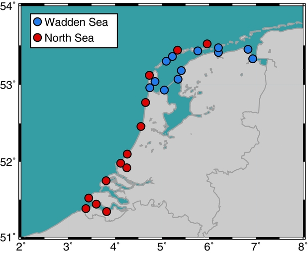
Reconstructed region-mean sea-level curves and accompanying linear trends for the Wadden Sea and the Dutch North Sea over 1958–2014. The region-mean sea-level curves have been filtered using a 12-month moving average.
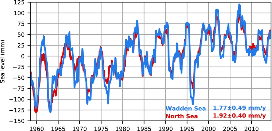
Monitoring vertical land motion of the Wadden Sea tide gauges
As tide gauges measure the sea level relative to a local benchmark on land, the observations also include (local) vertical land motion. In the Dutch Wadden Sea, (local) vertical land motion is introduced by, among others, gas extraction, salt mining and GIA. To be able to correct the observed water levels for these motions, a regular reconnection of the tide gauge zero to the tide gauge benchmark and to a reference level (e.g. Amsterdam Ordnance Datum / Normaal Amsterdams Peil for the Netherlands) is required. For the tide gauges located at the mainland of the Netherlands, the latter is established on a regular basis using spirit levelling. For the tide gauges on the Wadden Islands, spirit levelling cannot be used to establish the connection to the mainland, as spirit levelling cannot cross large water bodies.
The last first-order connection of the Wadden island (and offshore) tide gauges to the Normaal Amsterdams Peil (NAP) was established during the fifth precise levelling campaign using hydrostatic levelling between 1996 and 1999. After that there was a large second-order campaign in the Wadden Sea from 2000 until 2002 (the last using hydrostatic levelling). This campaign included the measurement locations at sea, north of the Wadden Islands (Texel Noordzee, Terschelling Noordzee, Wierumergronden and Huibersgat). At Oudeschild, Vlieland Haven and West-Terschelling, the tide gauges are connected to a first-order benchmark, hence their height was kept fixed, but tested in the pseudo-constrained least-squares adjustment.
In 2002, hydrostatic levelling was abandoned because it was believed that in the near future Global Navigation Satellite System (GNSS) techniques could take over. However, state-of-the-art quasi-geoid models covering the Dutch Wadden Sea only have centimetre accuracy (Farahani et al., Reference Farahani, Slobbe, Klees and Seitz2017). Consequently, no relative deformation of the local height networks at the Wadden Islands relative to the mainland NAP network can be observed. Relative vertical motions on the islands with respect to the first-order marks have been checked by local second-order levellings in 2009, though for Ameland and Schiermonnikoog there is no benchmark at the measurement location in the NAP database (second-order benchmarks are close by).
Alternatively, the vertical land motions are estimated from permanent GNSS measurements. However, in general the available GNSS measurement records in the Wadden Sea are too short. The longest record is available at Terschelling. Here, GNSS is available since 1996. Only since 2013/14 have the Wadden Sea tide gauges Oudeschild and Vlieland been equipped with permanent GNSS. Also on Ameland and Schiermonnikoog permanent GNSS is available (though maybe not connected to the tide gauge).
The satellite record
Satellite radar altimetry
Satellite radar altimeter observed sea-level variations in the North Sea are available for the TOPEX/Poseidon and Jason satellites with a near 10-day sampling interval. For the European Earth Observation satellites (ERS-1, ERS-2, Envisat), and the SARAL/AltiKa altimetry satellite mission (Envisat series), a total of c.40 tracks are available, with a sampling interval of 35 days. Statistically interpolated sea-level anomaly grids computed from altimetry observations are also available (AVISO, CCI). So far, however, only a limited number of studies (i.e. Madsen et al., Reference Madsen, Murray, Andersen and Pejrup2007; Sterlini et al., Reference Sterlini, Le Bars, de Vries and Ridder2017) have used the altimeter data record to study long-term variations or trends in the North Sea.
In coastal waters (which applies to the whole Wadden Sea), altimeter-derived sea surface heights become less accurate because (i) the observed waveforms are contaminated by reflections from land (remember that the typical beam-limited footprint size of pulse-limited radars is 7.5–10km), (ii) due to different sea states, observed waveforms differ from those on open ocean, (iii) the accuracy of the wet troposphere corrections is degraded and (iv) the accuracy of ocean tide corrections obtained from global ocean tide models is degraded (Vignudelli et al., Reference Vignudelli, Kostianoy, Cipollini and Benveniste2011). Conventional altimeters, like those from the TOPEX/Poseidon–Jason and Envisat series – are therefore not suitable to obtain sea surface heights in the Wadden Sea. Dedicated processing techniques might help to get closer to the shore (Passaro et al., Reference Passaro, Cipollini, Vignudelli, Quartly and Snaith2014; Roscher et al., Reference Roscher, Uebbing and Kusche2017), but their improvements are marginal or require a specific set of conditions to be able to work.
With the new type of altimeters on board the Cryosat-2 and Sentinel-3 missions, launched in 2010 and 2016 respectively, closed-burst unfocused Synthetic Aperture Radar (SAR) is applied to reduce the footprint in the along-track direction to 300–400 m (Wingham et al., Reference Wingham, Francis, Baker, Bouzinac, Brockley, Cullen, de Chateau-Thierry, Laxon, Mallow, Mavrocordatos, Phalippou, Ratier, Rey, Rostan and Viau2006). This makes it possible to observe sea level close to the coast, but in the Wadden Sea it is still problematic. Further enhancements are expected by applying fully focused SAR algorithms, which is possible for Cryosat-2 and Sentinel-3&6. With this technique the along-track footprint is further reduced to ~0.5m. The dynamic ocean surface decorrelates the signal over the ocean, so that effectively the footprint will be at least several tens of metres, but it will help to remove signals from static scatters on the land surface. Eventually, the Surface Water and Ocean Topography (SWOT) mission will provide 120km swaths of sea surface heights, with a horizontal resolution of several hundred metres. This mission will capture large parts of the Wadden Sea instantaneously.
Currently, even the new altimetry missions are not able to provide reliable sea-level change estimates in the Wadden Sea. Firstly, their records are too short to estimate reliable trends. Secondly, a proper tide model for the Wadden Sea is required to remove the effect of ocean tides, because they alias into the altimetry estimates. Thirdly, not enough research is done to state anything about the performance of altimeters in the Wadden Sea. From reconstructions it appears that sea level in the Wadden Sea closely follows the sea level in the North Sea, so it can act as a proxy. The main contribution of the new altimeter technologies is the possibility of validating instantaneous sea surface heights in models.
Mass changes from satellite gravimetry
Currently, no studies have attempted to directly estimate ocean mass changes from the Gravity Recovery And Climate Experiment (GRACE) satellite alone in the North Sea, although Frederikse et al. (Reference Frederikse, Riva, Kleinherenbrink, Wada, Broeke and Marzeion2016a) showed that the mass signal from GRACE correlates with the estimated tide-gauge observations. The limited spatial resolution of GRACE makes it prone to leakage, meaning that land hydrology signals and ocean changes in the North Sea basin are difficult to distinguish. The effect of leakage can be reduced using land hydrology models, but this requires accurate knowledge of the man-controlled water levels in the surrounding regions. Standard gridded ocean bottom pressure data are not suited to determine the mass changes in the North Sea, because they apply 500km Gaussian filters, which are larger than the North Sea itself (Chambers & Bonin, Reference Chambers and Bonin2012). A partitioning of the sea level in the North Sea has been done on the basis of a combination of GRACE data and altimetry (Rietbroek et al., Reference Rietbroek, Brunnabend, Kusche, Schröter and Dahle2016). Figure 19 reconfirms the large fluctuations in ocean bottom pressure on the shelf which contaminates the smoother signals originating from glaciers, ice caps and terrestrial hydrology.
Estimated sea-level contributions in the North Sea from a combination of GRACE and Jason-1/2 altimeter data. The variability in the North Sea is mostly dominated by ocean bottom pressure changes, which induce the largest uncertainties in the estimated trends (from Rietbroek et al., Reference Rietbroek, Brunnabend, Kusche, Schröter and Dahle2016, supplement).
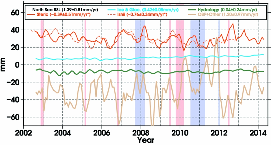
A local sea-level budget for the Wadden Sea
If all processes that affect sea-level change in the Wadden Sea are understood well, the sum of these processes should be equal to the observed sea-level change. Here, we combine the effects of wind, pressure, large-scale ocean dynamics, GIA, the nodal cycle, and present-day mass redistribution to reconstruct sea-level change in the Wadden Sea and compare the reconstructed curve to the tide-gauge observations (Fig. 20). The majority of the variability is caused by the effects of winds and the dynamic response to longshore wind, as discussed above, while mass redistribution and the nodal cycle show substantially less variability. When added together, the observed variability and trend in the Wadden Sea can be explained by the contributors (Fig. 20).
A sea-level budget for the Wadden Sea. (A) Individual contributors to sea-level changes in the Wadden Sea. The dynamic component, taken from Frederikse et al. (Reference Frederikse, Riva, Kleinherenbrink, Wada, Broeke and Marzeion2016a), consists of steric changes along the Portuguese coast and the Bay of Biscay. SLP stands for sea-level pressure. The mass redistribution term consists of the sum of all processes in Figure 10. All time series have been low-pass filtered using a 12e. The GIA component is estimated at 0.6mma−1, based on the global ICE6G-VM5a model (Peltier et al., Reference Peltier, Argus and Drummond2015). (B) Sum of all components in (A) versus the observed sea-level changes in the Wadden Sea.
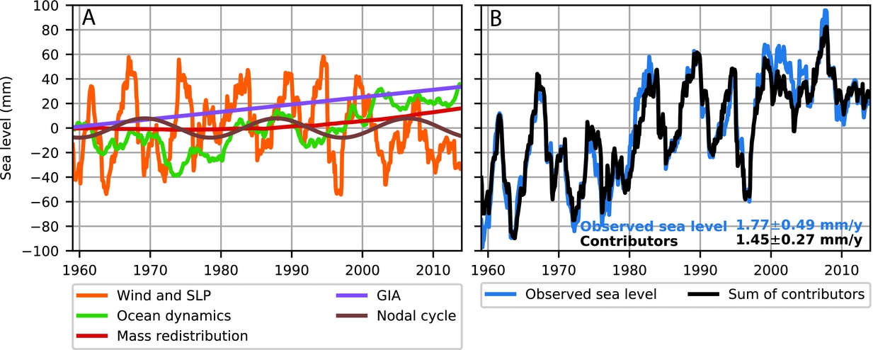
Regional sea-level change projections for the North Sea and the Wadden Sea
In this section, we provide an overview of sea-level projections for the 21st century, focusing on the Wadden Sea area (Fig. 21). The regional sea-level projections from IPCC AR5 (Church et al., Reference Church, Clark, Cazenave, Gregory, Jevrejeva, Levermann, Merrifield, Milne, Nerem, Nunn, Payne, Pfeffer, Stammer, Unnikrishnan, Stocker, Qin, Plattner, Tignor, Allen, Boschung, Nauels, Xia, Bex and Midgley2013) are taken as the starting point of this assessment. These projections include ocean steric and dynamic changes, ice-sheet and glacier mass changes, changes in land-water storage due to groundwater extraction, atmospheric pressure change and GIA.
The Dutch part of the Wadden Sea World Heritage area and the location of the two tide-gauge stations used (map adapted from www.waddensea-worldheritage.org).

While there has been progress in understanding most of the contributions, a recent development is that the dynamic ice-sheet contribution from Antarctica has now been connected to a Representative Concentration Pathway (RCP, Moss et al., Reference Moss, Edmonds, Hibaard, Manning, Rose, van Vuuren, Carter, Emori, Kainuma, Kram, Meehl, Mitchell, Nakicenovic, Riahi, Smith, Stouffer, Thomson, Weyant and Wilbanks2010) scenario (e.g. Levermann et al., Reference Levermann, Winkelmann, Nowicki, Fastook, Frieler, Greve, Hellmer, Martin, Meinshausen, Mengel, Payne, Pollard, Sato, Timmermann, Wang and Bindschadler2014; Golledge et al., Reference Golledge, Kowalewski, Naish, Levy, Fogwill and Gasson2015; Ritz et al., Reference Ritz, Edwards, Durand, Payne, Peyaud and Hindmarsh2015; DeConto & Pollard, Reference DeConto and Pollard2016). We also consider different GIA estimates and evaluate the impact this has on our regional sea-level projections. Subsidence in the Wadden Sea is not included in this section, but discussed in detail in Fokker et al. (Reference Fokker, Van Leijen, Orlic, Van der Manel and Hanssen2018).
Data and methods
The regional sea-level projections presented here are based on the materials and methods described in the IPCC AR5 (Church et al., Reference Church, Clark, Cazenave, Gregory, Jevrejeva, Levermann, Merrifield, Milne, Nerem, Nunn, Payne, Pfeffer, Stammer, Unnikrishnan, Stocker, Qin, Plattner, Tignor, Allen, Boschung, Nauels, Xia, Bex and Midgley2013) and the regional sea-level projections of Cannaby et al. (Reference Cannaby, Palmer, Howard, Bricheno, Calvert, Krijnen, Wood, Tinker, Bunney, Harle, Saulter, O'Neill, Bellingham and Lowe2016). Our starting point is the projected contributions to global mean sea level from ice-sheet changes, glacier mass loss, changes in land-water storage due to groundwater extraction and global thermal expansion made available in the IPCC AR5 supplementary data files (available from http://www.climatechange2013.org/report/full-report). The time series for ice-sheet, glacier and groundwater storage changes are combined with estimates of the corresponding sea-level ‘fingerprints’ that account for the responses of Earth's geoid (via gravity and rotational effects) and the lithosphere (Slangen et al., Reference Slangen, Carson, Katsman, van de Wal, Koehl, Vermeersen and Stammer2014) to obtain the associated regional sea-level change. We also include an estimate of relative sea-level change as a result of the vertical land motion and geoid changes associated with GIA from the ICE-5G (VM2) model (as described in Peltier, Reference Peltier2004). The final step in the regional projections is to account for local changes in the shape of the sea surface that can arise from local changes in circulation and/or density (‘oceanographic’ sea level). Following previous authors (e.g. Perrette et al., Reference Perrette, Landerer, Riva, Frieler and Meinshausen2013; Bilbao et al., Reference Bilbao, Gregory and Bouttes2015) we adopt a pattern-scaling type approach by computing linear regression coefficients between local oceanographic sea level and global thermal expansion (see Cannaby et al., Reference Cannaby, Palmer, Howard, Bricheno, Calvert, Krijnen, Wood, Tinker, Bunney, Harle, Saulter, O'Neill, Bellingham and Lowe2016, their fig. A1) using the same set of CMIP5 climate models (phase 5 of the Coupled Model Intercomparison Project, Taylor et al., Reference Taylor, Stouffer and Meehl2012) as Slangen et al. (Reference Slangen, Carson, Katsman, van de Wal, Koehl, Vermeersen and Stammer2014) and Church et al. (Reference Church, Clark, Cazenave, Gregory, Jevrejeva, Levermann, Merrifield, Milne, Nerem, Nunn, Payne, Pfeffer, Stammer, Unnikrishnan, Stocker, Qin, Plattner, Tignor, Allen, Boschung, Nauels, Xia, Bex and Midgley2013) (Table 3). We make the same assumptions about correlation of uncertainties as documented by Church et al. (Reference Church, Clark, Cazenave, Gregory, Jevrejeva, Levermann, Merrifield, Milne, Nerem, Nunn, Payne, Pfeffer, Stammer, Unnikrishnan, Stocker, Qin, Plattner, Tignor, Allen, Boschung, Nauels, Xia, Bex and Midgley2013) and Cannaby et al. (Reference Cannaby, Palmer, Howard, Bricheno, Calvert, Krijnen, Wood, Tinker, Bunney, Harle, Saulter, O'Neill, Bellingham and Lowe2016), except that the variance for global thermal expansion and a variance for the regression slope are estimated separately and combined assuming that there is no correlation between the two. Comparisons of the two approaches for a number of example locations have shown that this is a reasonable assumption (Cannaby et al., Reference Cannaby, Palmer, Howard, Bricheno, Calvert, Krijnen, Wood, Tinker, Bunney, Harle, Saulter, O'Neill, Bellingham and Lowe2016).
CMIP5 models (Taylor et al., Reference Taylor, Stouffer and Meehl2012) used for the projections in this paper, indicating the availability of model data per scenario.
Sea-level change projections
Time series of the global mean and the North Sea region
The global-mean ensemble-mean sea-level projections for 1986–2005 to 2081–2100 (the time periods used in IPCC AR5) based on Church et al. (Reference Church, Clark, Cazenave, Gregory, Jevrejeva, Levermann, Merrifield, Milne, Nerem, Nunn, Payne, Pfeffer, Stammer, Unnikrishnan, Stocker, Qin, Plattner, Tignor, Allen, Boschung, Nauels, Xia, Bex and Midgley2013) and Cannaby et al. (Reference Cannaby, Palmer, Howard, Bricheno, Calvert, Krijnen, Wood, Tinker, Bunney, Harle, Saulter, O'Neill, Bellingham and Lowe2016) are 0.44±0.17m for RCP2.6, 0.53±0.18m for RCP4.5 and 0.74±0.23m for the RCP8.5 scenario. The time series for each of these scenarios is presented in Figure 22A, B and C. In all three scenarios, the thermal expansion contribution is the largest of the individual contributions (in red). The glacier contribution and the ice-sheet surface mass balance contributions are smaller and dependent on the choice of scenario. In IPCC AR5, the ice dynamics contributions and the groundwater contribution were assumed to be scenario-independent, with the exception of Greenland dynamics in the RCP8.5 scenario to represent larger outflow.
Projected sea-level change in Global Mean (A, B, C), Den Helder (D, E, F) and Delfzijl (G, H, I), for the RCP2.6 (A, D, G), RCP4.5 (B, E, H) and RCP8.5 (C, F, I) scenarios. Shown are the individual contributions (coloured lines) and the total change (black line and shading, 5–95%). The model ensemble is based on CMIP5 models (Table 3).
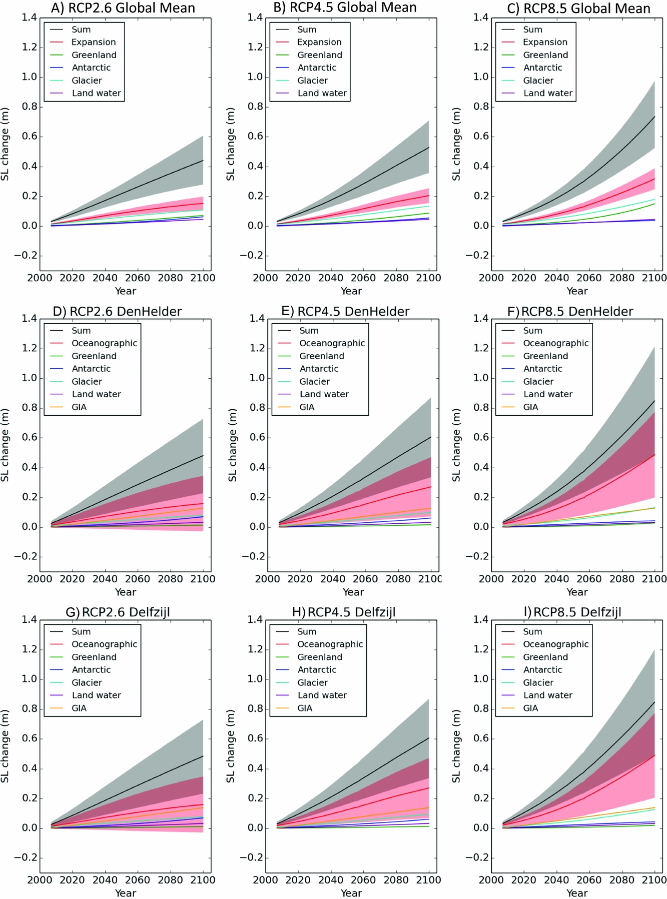
On a regional scale, Den Helder (Fig. 22D, E and F) and Delfzijl (Fig. 22G, H and I) are similar to each other, but they differ from the global mean projections. The thermal expansion contribution is now included in the ‘oceanographic’ contribution (red), which also includes changes in ocean dynamics and atmospheric pressure loading. Both the magnitude of the change and the uncertainty in this contribution are larger than in the global mean. The increased uncertainty in the ocean component is mainly caused by larger variability on a regional scale due to the different phasing and larger regional response to annual, interannual and decadal variability (such as the El Niño Southern Oscillation (ENSO)), which is averaged out in the global mean.
The steric component of sea-level rise is larger in the North Atlantic compared to the global mean because, as climate warms up, the mid-latitude oceans become both warmer than high-latitude oceans and fresher due to increased precipitation compared to equatorial oceans. These two effects decrease the density of the water (Bouttes et al., Reference Bouttes, Gregory, Kuhlbrodt and Smith2014). Additionally, a reduction of the Atlantic Meridional Overturning Circulation (AMOC) strength is found in models participating in CMIP5. This indirect effect tends to reduce the direct effect of surface heating and freshening, but it is not dominant (Bouttes et al., Reference Bouttes, Gregory, Kuhlbrodt and Smith2014). The large-scale ocean circulation system is expected to weaken in a warmer climate (Gregory et al., Reference Gregory, Dixon, Stouffer, Weaver, Driesschaert, Eby, Fichefet, Hasumi, Hu, Jungclaus, Kamenkovich, Levermann, Montoya, Murakami, Nawrath, Oka, Sokolov and Thorpe2005) and will lead to higher sea levels in the northern North Atlantic (Levermann et al., Reference Levermann, Griesel, Hofmann, Montoya and Rahmstorf2005), although the effect of rising global temperatures on the development of the AMOC is not yet fully quantified, which results in an enhanced uncertainty for future dynamic sea-level changes in the North Sea.
In the future, as the Greenland Ice Sheet continues to melt, the freshwater export will also contribute to sea-level rise in the North Atlantic and in the North Sea. Assuming a modest mass loss from Greenland equivalent to a global mean sea-level rise of 10cm during the 21st century, Slangen & Lenaerts (Reference Slangen and Lenaerts2016) showed that this freshwater effect would raise sea level by an additional 5–10cm locally in the North Sea. This process is not yet included in the CMIP5 models used here to project dynamical sea-level changes (Lenaerts et al., Reference Lenaerts, Le Bars, van Kampenhout, Vizcaino, Enderlin and van den Broeke2015), so that it needs to be added to the numbers given in Table 4.
Cumulative sea-level change in metres (5–95%) for the 1986–2005 mean vs the 2081–2100 mean for Den Helder and Delfzijl.
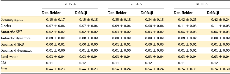
The regional mass contribution of the Greenland Ice Sheet in the North Sea is nearly zero (as opposed to the density effect mentioned above), which is well below the global mean, as a result of the gravitational effect. Also for the glacier contribution, the contribution at the Dutch coast is below the global mean due to the gravitational effect, as most glacier areas are located in the Northern Hemisphere. For Antarctica, the gravitational effect works the other way. As the Netherlands are in the far field of Antarctica, the regional contribution is larger than the global mean. Both the glacier and the land water contribution are affected by the gravitational fingerprints, but the regional effect is close to the global average for both. The GIA contribution has a negligible global mean effect on sea-level change, but it can have a distinct regional effect. Using the ICE5G GIA model, for Delfzijl and Den Helder, the effect of GIA is a relative sea-level rise as a result of a sinking solid earth (0.11–0.12m over the 21st century; Fig. 22; Table 4). See below for a discussion on the differences between GIA models and modelling methods.
The larger uncertainty in the regional oceanographic contribution translates into a larger uncertainty for the summed sea-level projections at the Den Helder and Delfzijl grid points (Fig. 22). The projected changes by 2100 for these two locations are above the global mean projections (+0.04, +0.08 and +0.11m for the three RCP scenarios, respectively), mainly due to the addition of the GIA contribution in the regional projections.
Both globally and regionally, the total sea-level projections show the impact of the RCP scenario (Fig. 23), with RCP2.6 as the low- and RCP8.5 as the high-emission scenario. However, although the projections’ means diverge, their uncertainties still overlap by the end of the century, with a larger overlap for the regional projections (Table 5). This is caused by the RCP scenarios that drive the climate models: they do not diverge until the middle of the 21st century.
(A) Global-mean reconstructed sea-level change (black, four different reconstructions) and projections for RCP2.6 (blue) and RCP8.5 (red) (2005–2100, 5–95%); (B) Tide-gauge observations vs local relative sea-level projections for Den Helder (C) Tide-gauge observations vs local relative sea-level projections for Delfzijl.
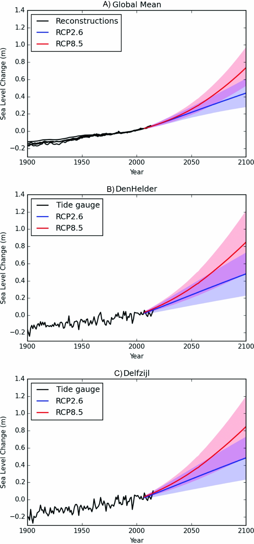
Cumulative sea-level change in metres (5–95%) for three periods, taking the mean of Den Helder and Delfzijl.
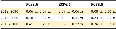
The projections shown in Figures 22 and 23 are largely based on the IPCC AR5 results (Church et al., Reference Church, Clark, Cazenave, Gregory, Jevrejeva, Levermann, Merrifield, Milne, Nerem, Nunn, Payne, Pfeffer, Stammer, Unnikrishnan, Stocker, Qin, Plattner, Tignor, Allen, Boschung, Nauels, Xia, Bex and Midgley2013). Since IPCC AR5, a lot of research has been done, updating various estimates of the contributions to sea-level change (summarised in e.g. Clark et al., Reference Clark, Church, Gregory and Payne2015; Slangen et al., Reference Slangen, Adloff, Jevrejeva, Leclercq, Marzeion, Wada and Winkelmann2017b). Estimates of the steric and dynamic contributions have not changed; these are taken from the CMIP5 model archive. New results are expected with the release of the sixth phase of the climate model intercomparison (CMIP6), which will include new developments in the climate models, such as interactive ice sheets, but these are not available yet. Updated glacier models and newly developed models simulate generally lower glacier contributions (Marzeion et al., Reference Marzeion, Jarosch and Hofer2012; Huss & Hock, Reference Huss and Hock2015; Slangen et al., Reference Slangen, Adloff, Jevrejeva, Leclercq, Marzeion, Wada and Winkelmann2017b), although only by a couple of centimetres in 2100.
In recent years, particularly the Antarctic dynamic ice sheet contribution has sparked debate in the scientific community. It is potentially the largest contribution to sea-level rise, but the uncertainties in the processes, timing and magnitude of the contribution are large. So large, in fact, that in IPCC AR5, the state of the science did not allow for a scenario dependence of this contribution. Now, several estimates based on different methods and approaches are available (Fig. 24).
Sensitivity of sea-level projections to different RCP8.5-based estimates of the Antarctic contribution. IPCC AR5 Antarctic contribution vs four post-AR5 estimates: (A) Levermann et al. (Reference Levermann, Winkelmann, Nowicki, Fastook, Frieler, Greve, Hellmer, Martin, Meinshausen, Mengel, Payne, Pollard, Sato, Timmermann, Wang and Bindschadler2014, Ice Dynamics only), (B) Golledge et al. (Reference Golledge, Kowalewski, Naish, Levy, Fogwill and Gasson2015, Surface Mass Balance and Ice Dynamics), (C) Ritz et al. (Reference Ritz, Edwards, Durand, Payne, Peyaud and Hindmarsh2015, Ice Dynamics only) and (D) DeConto & Pollard (Reference DeConto and Pollard2016, Surface Mass Balance and Ice Dynamics). (E) Total global mean sea-level projections (RCP8.5) combined with each of the Antarctic estimates.

The Sea-level Response to Ice Sheet Evolution (SeaRise) intercomparison project (Bindschadler et al., Reference Bindschadler, Nowicki, Abe-Ouchi, Aschwanden, Choi, Fastook, Granzow, Greve, Gutowski, Herzfeld, Jackson, Johnson, Khroulev, Levermann, Lipscomb, Martin, Morlighem, Parizek, Pollard, Price, Ren, Saito, Sato, Seddik, Seroussi, Takahashi, Walker and Wang2013; Fig. 24A) specifically aimed at comparing and quantifying the uncertainties in the ice discharge from Antarctica resulting from climate change forcing and oceanic response in a number of ice sheet models (Levermann et al., Reference Levermann, Winkelmann, Nowicki, Fastook, Frieler, Greve, Hellmer, Martin, Meinshausen, Mengel, Payne, Pollard, Sato, Timmermann, Wang and Bindschadler2014). They found a median contribution of 0.09m (0.01–0.37m, 90%) for the RCP8.5 scenario, which is close to the IPCC values but has a skewed probability distribution to larger values. Using a coupled ice-sheet/ice-shelf model, Golledge et al. (Reference Golledge, Kowalewski, Naish, Levy, Fogwill and Gasson2015) found a reduction of buttressing ice shelves leading to increased discharge and flow acceleration in all scenarios except RCP2.6. Under RCP8.5 (Fig. 24B), they projected a contribution of 0.1–0.39m by 2100, which is well above the IPCC AR5 estimates. They also showed that a collapse of the major ice shelves might trigger a much larger commitment to sea-level rise on centennial to millennial timescales. Ritz et al. (Reference Ritz, Edwards, Durand, Payne, Peyaud and Hindmarsh2015) used a process-based statistical approach and projected a contribution of up to 0.3m by 2100 (Fig. 24C), mainly driven by a contribution from marine ice-sheet instability (MISI) in the Amundsen Sea Embayment. The projected contribution is therefore slightly larger than the IPCC AR5 and in addition they found slightly skewed probability distributions to higher values. Using an ice-sheet/ice-shelf model that includes marine ice-cliff instability and hydrofracturing, DeConto & Pollard (Reference DeConto and Pollard2016) projected a much larger contribution of 1.05±0.30m by 2100 under RCP8.5 (Fig. 24D).
When comparing the effects of the four previously described estimates on the total sea-level projections (focusing on the median values, not the tails which would significantly change the uncertainty band; Fig. 24E), it is clear that even though most of the post-AR5 contributions for Antarctica tend to be larger than in the IPCC AR5, it will be difficult to reconcile the different estimates into a single ‘best estimate’ because they are too far apart. However, research by Kuipers Munneke et al. (Reference Kuipers Munneke, Ligtenberg, van Den Broeke and Vaughan2014) finds that hydrofracturing will take place on longer timescales than suggested by DeConto & Pollard (Reference DeConto and Pollard2016). Further research is needed to determine realistic timescales and magnitudes for the processes involved in dynamic ice sheet mass loss.
As each GIA model is constrained using different ice histories and assuming different solid-earth rheologies, the choice of GIA model can make a difference in local sea-level projections (Fig. 6). Since IPCC AR5, a follow-up of the ICE-5G (VM2) model (Peltier, Reference Peltier2004) has been released: the ICE-6G (VM2a) model (Peltier et al., Reference Peltier, Argus and Drummond2015). This results in a larger sea-level rise contribution along the Dutch coast, with differences in the order of 1mma−1. The difference to the ANU model (updated from Lambeck et al, Reference Lambeck, Smither and Johnston1998; Fig. 25C) is even larger since the uplift affects a larger region than in the ICE-xG models. Over the 21st century as a whole, this adds up to a considerable 10–30cm difference between the GIA models. Regional GIA models, as presented in Figure 6, may be better constrained but are not suitable to use in the model set-up here which requires a global sea-level projection framework.
Overview of sea-level projections presented in literature since IPCC AR5, sorted by RCP scenario, translated into regional projections for Den Helder (m, 2005–2100), showing median, 17–83% (light inner bars) and 5–95% (dark outer bars). *The 5–95% spread of the IPCC AR5 projections corresponds to the likely range.
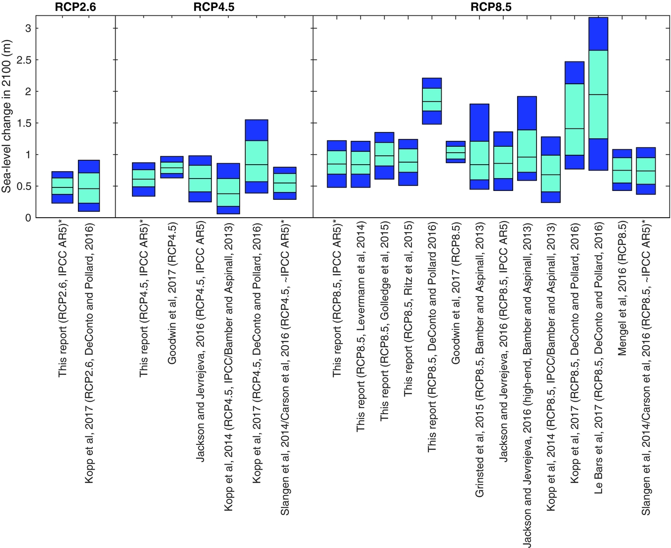
Sea-level change projections for 2100
In IPCC AR5, future global sea-level rise is assessed as likely (P>66%) to be within the range of the projections. However, not having information on the complete probability distribution of future sea-level change presents a challenge for policy-makers and coastal planners: it is often important to know what the high-end or extreme sea-level change will be, in the upper tails of the uncertainty distribution. Some publications post AR5 have therefore attempted to try and quantify a larger range of the probability distribution, often making use of expert elicitations to quantify the future ice-sheet contribution (e.g. Bamber & Aspinall, Reference Bamber and Aspinall2013; Jevrejeva et al., Reference Jevrejeva, Moore, Grinsted, Matthews and Spada2014; Kopp et al., Reference Kopp, Horton, Little, Jerry, Oppenheimer, Rasmussen, Strauss and Tebaldi2014; Grinsted et al., Reference Grinsted, Jevrejeva, Riva and Dahl-Jensen2015). At the same time there has also been progress in our understanding of sea-level change (e.g. see reviews by Clark et al., Reference Clark, Church, Gregory and Payne2015; Slangen et al., Reference Slangen, Adloff, Jevrejeva, Leclercq, Marzeion, Wada and Winkelmann2017b) and, most notably, there have been recent developments in the projections of ice-mass changes in Antarctica (e.g. Ritz et al., Reference Ritz, Edwards, Durand, Payne, Peyaud and Hindmarsh2015; DeConto & Pollard, Reference DeConto and Pollard2016).
Here we compare different types of regional sea-level projections for the Wadden Sea (Fig. 25). We show projections based on IPCC AR5 science and also projections that have been published since the release of IPCC AR5. The projections can be roughly categorised as follows: (i) projections from IPCC AR5 or based on IPCC AR5 science (Slangen et al., Reference Slangen, Katsman, Wal, Vermeersen and Riva2012, Reference Slangen, Carson, Katsman, van de Wal, Koehl, Vermeersen and Stammer2014; Cannaby et al., Reference Cannaby, Palmer, Howard, Bricheno, Calvert, Krijnen, Wood, Tinker, Bunney, Harle, Saulter, O'Neill, Bellingham and Lowe2016; KNMI, 2017); (ii) projections that we construct by making use of the median of recent projections from ice-sheet models (Levermann et al., Reference Levermann, Winkelmann, Nowicki, Fastook, Frieler, Greve, Hellmer, Martin, Meinshausen, Mengel, Payne, Pollard, Sato, Timmermann, Wang and Bindschadler2014; Golledge et al., Reference Golledge, Kowalewski, Naish, Levy, Fogwill and Gasson2015; Ritz et al., Reference Ritz, Edwards, Durand, Payne, Peyaud and Hindmarsh2015; DeConto & Pollard, Reference DeConto and Pollard2016) – note that these ice-sheet projections have skewed uncertainty distributions which are not included here; and (iii) projections that make use of expert elicitations or a semi-empirical approach (Kopp et al., Reference Kopp, Horton, Little, Jerry, Oppenheimer, Rasmussen, Strauss and Tebaldi2014; Grinsted et al., Reference Grinsted, Jevrejeva, Riva and Dahl-Jensen2015; Jackson & Jevrejeva, Reference Jackson and Jevrejeva2016; Mengel et al., Reference Mengel, Levermann, Frieler, Robinson, Marzeion and Winkelmann2016).
The main difference between these studies is how the ice-sheet contribution is handled. There are, however, also other differences in the methodologies applied which give different results. For example, Mengel et al. (Reference Mengel, Levermann, Frieler, Robinson, Marzeion and Winkelmann2016) show noticeable differences between their results and those given in IPCC AR5 for the separate contributions to future sea-level rise. The treatment and presentation of uncertainties is also different between the projections. As mentioned, the spread of the IPCC AR5 projections is based on a likely range, whereas most other projections shown here are presented with corresponding 5–95% uncertainties (e.g. Kopp et al., Reference Kopp, Horton, Little, Jerry, Oppenheimer, Rasmussen, Strauss and Tebaldi2014; Grinsted et al., Reference Grinsted, Jevrejeva, Riva and Dahl-Jensen2015; Jackson & Jevrejeva, Reference Jackson and Jevrejeva2016; Mengel et al., Reference Mengel, Levermann, Frieler, Robinson, Marzeion and Winkelmann2016; Le Bars et al., Reference Le Bars, Drijfhout and de Vries2017).
At the request of the Dutch Delta Committee (Kabat et al., Reference Kabat, Jacobs, Hutjes, Hazeleger, Engelmoer, Witte, Roggema, Lammerts, Bessembinder, Hoekstra and van den Berg2009), high-end sea-level change along the Dutch coast was assessed in 2008. The results were presented in a report by Vellinga et al. (Reference Vellinga, Katsman, Sterl, Beersma, Hazeleger, Church, Kopp, Kroon, Oppenheimer, Plag, Rahmstorf, Lowe, Ridley, von Storch, Vaughan, van de Wal, Weisse, Kwadijk, Lammersen and Marinova2009) and a peer-reviewed publication by Katsman et al. (Reference Katsman, Sterl, Beersma, van den Brink, Church, Hazeleger, Kopp, Kroon, Kwadijk, Lammersen, Lowe, Oppenheimer, Plag, Ridley, von Storch, Vaughan, Vellinga, Vermeersen, van de Wal and Weisse2011). Their high-end scenario added up to 0.55–1.15m global mean sea-level change between 1990 and 2100. Their method builds on the IPCC AR4 methodology (Meehl et al., Reference Meehl, Stocker, Collins, Friedlingstein, Gaye, Gregory, Kitoh, Knutti, Murphy, Noda, Raper, Watterson, Weaver, Zhao, Solomon, Qin, Manning, Chen, Marquis, Averyt, Tignor and Mille2007) and KNMI (Koninklijk Nederlands Meteorologisch Instituut) scenarios (Van den Hurk et al., Reference Van den Hurk, Klein Tank, Lenderink, van Ulden, van Oldenborgh, Katsman, van den Brink, Keller, Bessembinder, Burgers, Komen, Hazeleger and Drijfhout2006). The projections included steric/dynamic changes based on CMIP3 models, glacier estimates based on volume–area modelling, and ice-sheet estimates based on models, expert estimates and observed changes. In the ‘severe’ scenario, this included a collapse of ice shelves in the Amundsen Sea Embayment and accelerated melting of glaciers on East Antarctica and the Antarctic Peninsula, and a doubling of Greenland tidewater glacier discharge by 2050. The projected change presented in this report is 0.76±0.36m for the RCP8.5 scenario along the Dutch coast (from 2018 to 2100; Table 5), compared to 0.74±0.35m from the Delta Committee (from 1990 to 2100). However, if the observed trends between 1990 and 2018 are taken into account, the Delta Committee central estimate of 0.74m would translate to 0.66–0.70m for the 2018–2100 period. The differences between the Delta Commission report and this paper are primarily in the steric/dynamic contribution and glacier contribution, which almost double in RCP8.5. The Antarctic contribution of this paper falls within the range of Katsman et al. (Reference Katsman, Sterl, Beersma, van den Brink, Church, Hazeleger, Kopp, Kroon, Kwadijk, Lammersen, Lowe, Oppenheimer, Plag, Ridley, von Storch, Vaughan, Vellinga, Vermeersen, van de Wal and Weisse2011), but is at the lower bound. However, if the results of DeConto & Pollard (Reference DeConto and Pollard2016) are included in the projections, the total global mean sea-level projection is c.1.7m (median value, Fig. 24E), which is considerably larger than the high-end estimate of the Delta Committee. This is in line with other publications focusing on high-end sea-level estimates, such as Jevrejeva et al. (Reference Jevrejeva, Moore, Grinsted, Matthews and Spada2014), who find high-end global mean change in the order of 1.8–2.5m by 2100 (high-end only results are not included in Fig. 25).
Variability around projected sea-level rise
The projections discussed in the previous sections are all long-term and do not take local small-scale variability into account. Here, we combine the observed variability from the tide-gauge stations with the projections to show the local differences on shorter timescales. We use tide-gauge observations for the period 1865–2015 to estimate the local variability and assume that the distribution of the variability does not change in the future (Church et al., Reference Church, Clark, Cazenave, Gregory, Jevrejeva, Levermann, Merrifield, Milne, Nerem, Nunn, Payne, Pfeffer, Stammer, Unnikrishnan, Stocker, Qin, Plattner, Tignor, Allen, Boschung, Nauels, Xia, Bex and Midgley2013; Sterl et al., Reference Sterl, Bakker, van den Brink, Haarsma, Stepek, Wijnant and de Winter2015).
The rates of change measured at the tide-gauge stations have a wide distribution. Detrended yearly rates vary between −111 and 151mma−1 for Delfzijl and between −100 and 89mma−1 for Den Helder. The variability reduces as averages are taken over longer periods: detrended 10-year running means vary between −35 and 41mma−1 for Delfzijl and −35 and 22mma−1 for Den Helder (Fig. 26, black bars). The distribution is wider for the Delfzijl tide-gauge station compared to Den Helder.
Probability distribution of the linearly detrended 10-year running mean tide-gauge rates (mma−1, 1865–2015, black); combined with local sea-level rise projection rates (mma−1) of the lower 5% bound of RCP2.6 (red colours) and the upper 95% bound of RCP8.5 (blue colours) for Den Helder (upper row) and Delfzijl (lower row), for the years 2030 (left), 2050 (centre) and 2100 (right).
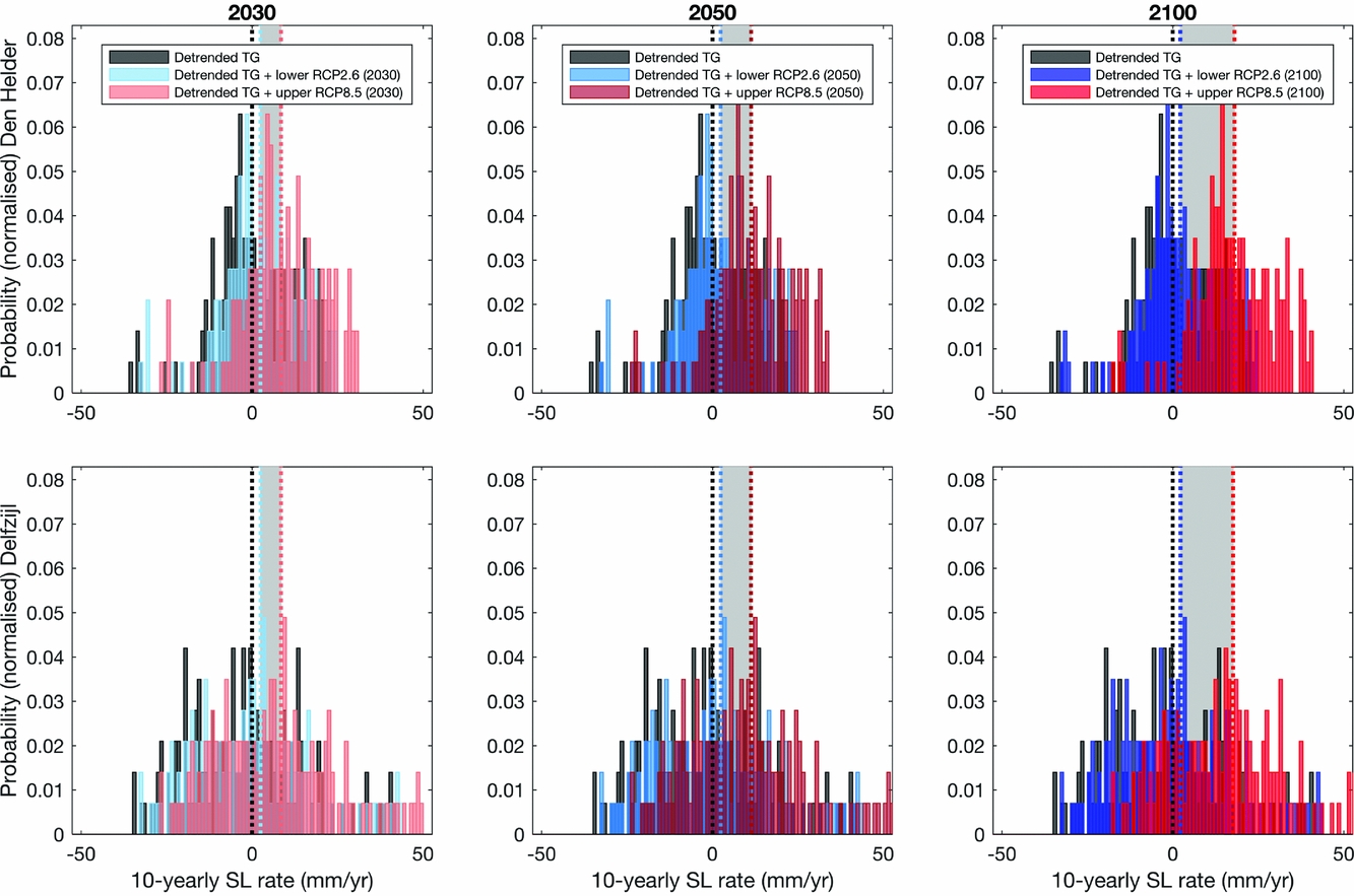
The observed distribution shifts by c.2mma−1 when the RCP2.6 lower 5th percentile projected sea-level rate is added (also averaged over 10 years) and it stays relatively constant for the years 2030, 2050 and 2100 (Table 6; Fig. 26, blue). For the RCP8.5 upper 95th percentile, the projected rates double between 2030 and 2100, from c.9mma−1 to c.18mma−1 (Table 6; Fig. 26, red). Given the relatively large spread in the observed rates (standard deviation of 17mm for Delfzijl and 11mm for Den Helder), RCP2.6 projected rates cause no significant change in the distribution, but the projected rates of RCP8.5 in 2050 and 2100 cause a more significant shift larger than 1 standard deviation.
Projected yearly sea-level rates (mma−1) for the lower 5% bound of RCP2.6 and the upper 95% bound of RCP8.5 for Den Helder and Delfzijl.
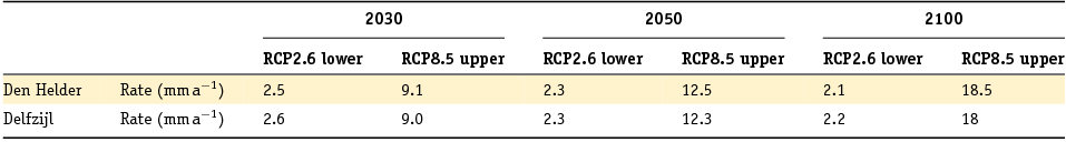
A major driver of variability in sea level is the extremes from storm surges. Arns et al. (Reference Arns, Wahl, Dangendorf and Jensen2015) argued that for the northern part of the German Bight, in the case of a sea-level rise of 54cm, nonlinear tidal effects lead to an increase of extreme storm-surge sea levels by up to 15cm (in addition to the mean sea-level change). This conclusion was extended to the Dutch part of the Wadden Sea by Idier et al. (Reference Idier, Paris, le Cozannet, Boulahya and Dumas2017), who showed that, for a mean sea-level rise of less than 2m, extreme sea-level events (annual maximum water level) proportionally increase by an additional 15% of the sea-level rise. This means that for a sea-level rise of 1m the annual maximum tidal water level increases by 1.15m.
However, this conclusion only holds for the case where locally the land is not allowed to flood. The increase is mostly cancelled in the case of flooding, showing that coastal protection decisions can have an impact on maximum sea level. Additionally, in regions of depth-limited waves like the Wadden Sea, an increase of the mean sea level also leads to an increase of the wave height. This effect lead Arns et al. (Reference Arns, Dangendorf, Jensen, Talke, Bender and Pattiaratchi2017) to argue that the design height of coastal protection for the German Bight will need to be 48–56% higher than it would be for only the mean sea-level rise. These numbers are obtained under the assumption that future extreme wind conditions will remain similar to those of the present day, which is what most climate models find (Sterl et al., Reference Sterl, Bakker, van den Brink, Haarsma, Stepek, Wijnant and de Winter2015). One major limitation of these models, however, is that their horizontal resolution is not high enough to solve for hurricanes. Using a high-resolution model, Haarsma et al. (Reference Haarsma, Hazeleger, Severijns, de Vries, Sterl, Bintanja, van Oldenborgh and van den Brink2013) showed that global warming could result in more hurricanes hitting western Europe, which could have large effects on extreme storm surges and wave conditions, and therefore impact the North Sea coast and the Wadden Sea area.
Time-variable sources of uncertainty in the projections
There are various sources of uncertainty that determine the total uncertainty in the projections. A main source of uncertainty is the internal climate variability: natural fluctuations in the climate. This includes large-scale phenomena like the ENSO or the NAO, which have an effect on interannual to interdecadal timescales. These fluctuations can be quite large, especially on a regional scale. Therefore, this is a major uncertainty in climate and sea-level projections on decadal timescales (Fig. 27): depending on the phasing of, for instance, ENSO, sea-level change can be reduced or amplified significantly (e.g. Boening et al., Reference Boening, Willis, Landerer, Nerem and Fasullo2012).
Sources of uncertainties in the sea-level projections on different timescales, considering internal variability (yellow), scenario uncertainty (green) and model uncertainty (blue). Decomposition of uncertainties follows the approach of Hawkins and Sutton (2009).
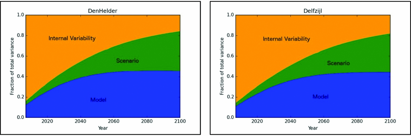
A second source of uncertainty in the projections is the choice of emission scenario, which is largely based on the actions taken by society. In the first few decades of the 21st century, the emission scenarios do not yet have a large effect on the projected sea-level change, as the response of the different processes contributing to sea level is delayed. However, from the mid-21st century onwards the projections as a result of the followed scenarios (RCP2.6, 4.5 or 8.5) start to diverge and therefore have a larger effect on the projected uncertainties (Fig. 27). This effect is expected to continue to increase past 2100, when the majority of the sea-level response will start to emerge.
A third source of uncertainty is the choice of the climate model used for the projections. There are 21 models, each with one model realisation, included in the ensemble of sea-level projections and there is a significant spread within this ensemble. This is due to a number of reasons, such as different model set-up or different parameterisations of sub-gridscale processes. Although in the 21st century initially the internal variability is the major source of uncertainty, the model uncertainty quickly grows to c.40% in 2050 and remains constant for the remainder of the period.
In order to reduce uncertainties in the projections, this analysis clearly shows that it is important to consider the period of interest: for 2030 the internal variability is the dominant source of uncertainty while the choice of scenario is much less relevant. However, reducing the model uncertainty would be a gain throughout the 21st century.
Discussion and way forward
Processes
On decadal and longer timescales, dynamic sea-level changes in the Wadden Sea appear to be coherent with North Sea sea-level changes. Hence, a thorough understanding of the major physical processes that affect sea level in the North Sea are of utmost importance to understand the behaviour of the Wadden Sea on longer timescales. Currently, the response of the North Sea to wind-driven coastally trapped waves is reasonably understood. However, next to this mode of decadal variability, multi-decadal variability due to large-scale oceanic features may reach the North Sea as well. In particular, the North Atlantic Ocean shows distinct multi-decadal variability signals (e.g. McCarthy et al., Reference McCarthy, Haigh, Hirschi, Grist and Smeed2015). However, it is not known whether and how the North Sea responds to these large-scale fluctuations. Furthermore, in a warming climate, the meridional overturning circulation may weaken (Levermann et al., Reference Levermann, Griesel, Hofmann, Montoya and Rahmstorf2005), which may also affect the North Sea and Wadden Sea. Strengthening the causal links between large-scale oceanic variability and local sea-level changes, by combining model results with physical understanding, forms a key challenge to understand contemporary and future sea-level changes.
On shorter temporal scales, sea-level changes are to a large extent driven by wind. The sea-level response to wind is affected by the local tidal regime, bathymetry, and time-mean sea-level changes. This combination results in wind-driven sea-level variability that is highly spatially variable. To maintain and ensure present and future safety during extreme surge events, knowledge is needed on how all these aforementioned factors affect sea-level changes. This knowledge becomes crucial under future sea-level change scenarios, since extremes may be amplified under rising mean sea level (Arns et al., Reference Arns, Dangendorf, Jensen, Talke, Bender and Pattiaratchi2017).
Observations
Palaeo-observations
To improve our understanding of past sea-level changes in the Wadden Sea and to be able to use them in improving GIA models and sea-level projections, we identify three focal areas for future research.
(1) Collecting high-quality sea-level index points and establishing nationwide databases.
The most-recent Wadden Sea sea-level reconstruction (Meijles et al., accepted) is significantly larger than GIA models of the 1990s (Lambeck et al., Reference Lambeck, Smither and Johnston1998) and Vink et al. (Reference Vink, Steffen, Reinhardt and Kaufmann2007). It is unknown whether this indicates a vertical offset in the index-point data, an offset in the calibration of the GIA models, or both. To investigate and resolve this inconsistency, additional basal-peat radiocarbon dates from carefully selected sites should be collected. The available sea-level index-point data should be kept in a database with national cover (i.e. following the protocols and guidelines in Hijma et al., Reference Hijma, Engelhart, Törnqvist, Horton, Hu, Hill, Shennan, Long and Horton2015), to make them more directly and more transparently usable between Holocene geologists and GIA modellers.
(2) Improving our understanding of the evolution of the Wadden Sea through time.
In the Netherlands most, if not all, sea-level index points are derived from palaeo-environments in dynamic and wide back-barrier settings that often extend for tens of kilometres in a landward direction. This means that for any period of time there is a large spatial variation in tidal parameters and that for any location these parameters can change rapidly due to a change in geometry of the tidal basin. This applies also to the Wadden Sea area, which has experienced rather dramatic changes in configuration during the last 8000 years. Getting a grip on the spatial and temporal changes in the tidal configuration is possible with a palaeo-tidal modelling effort that can help in refining the indicative range and hence can reduce the uncertainty around the relation of a sea-level indicator with past sea level.
(3) Improving GIA models with upgraded geological sea-level data.
The recent work of Meijles et al. (accepted) highlighted that there are still large discrepancies between the output of the GIA models and the actual sea-level data for the Holocene. Most GIA models find sea-level curves from the Rotterdam area systematically higher than those from the Wadden Sea area. At the same time, the data from Meijles et al. (accepted) could mean that in the last 7000 or 5000 years or so, the differential movement was negligible. This highlights the necessity for improved GIA modelling and upgrading of the observational datasets that it is iterated on, besides scrutiny and national databasing effort. Screening and reassessing the basal-peat index points from the North Sea offshore for clustering around periods of acceleration is a step to perform to reduce the undersampling of the North Sea. Such work has recently started, including a NIOZ Pelagia cruise shooting seismics and sampling identified patches of basal peats at critical depths, 10–100km off Vlieland. Especially the Dutch and German sectors of the southern North Sea hold important suitable records from this time period (Cohen et al., Reference Cohen, Westley, Erkens, Hijma, Weerts, Flemming, Harff, Moura, Burgess and Bailey2017). Sampling in the area between the Dutch mainland and Dogger Bank is important to constrain long-term components of subsidence (tectonic subsidence) and the long-term component of GIA modelling (residual effects of multiple cycles of GIA warping).
Present-day observations
Currently there is no operational technique available to connect the Wadden Islands to the NAP height system at the mainland. Consequently, any relative deformation of the local height networks at the Wadden Islands relative to the mainland NAP network cannot be observed. We propose the following recommendations for future research:
1) To develop a 3D hydrodynamic model for the Wadden Sea that includes all relevant physical processes and that is properly embedded in the observational network.
2) To exploit the possibilities offered by the new generation of SAR altimeters (available on the Cryosat-2 and Sentinel-3 missions) to provide the required resolution of sea surface height measurements in the Wadden Sea, and generating an altimeter-derived dataset of observed water levels that can be used to validate and calibrate the model.
3) To estimate the error variance–covariance matrix of the model-based MDT from which the error variance–covariance matrix of the MDT differences can be obtained. The latter information is needed to be able to combine the hydrodynamic levelling data with spirit levelling data.
Furthermore, interferometric Synthetic Aperture Radar (InSAR) may be used to detect relative vertical land motion, possibly aided by the use of strategically positioned corner reflectors and transponders. On a much larger scale, gravimetry missions such as GRACE and its follow-on provide estimates of large-scale mass-driven sea level in the larger North Sea. Optical and microwave satellite images, such as for example the SPOT series and the TerraSAR-X and Tandem-X satellites, respectively, may provide information on geomorphological features which change over time.
We therefore recommend promotion of pilot studies using remote sensing in the Wadden Sea in order to:
1. Benefit from spaceborne high temporal and spatial resolution information in the interior of the Wadden Sea.
2. Pave the way for operational uses of satellite data (e.g. data assimilation in operational models).
3. Identify the needs and requirements of national and regional stakeholders for future satellite missions.
Projections
The sea-level community requires input from other research communities to make sea-level projections. Large-scale changes in sea level in the long term will be driven by the response of the climate system to enhanced radiative forcing as a result of increased emission of greenhouse gases. Therefore it is important to develop process-based ice-dynamical models, in particular for the Antarctic contribution. This is required to investigate when and where the peak of sea-level rise will be, which in turn is relevant for policy-makers and coastal protection. In addition, the surface mass balance models of the ice sheets (and preferably also ice dynamic models) should be included in climate models such that the impact of additional freshwater forcing on the ocean dynamics can be studied. This is a development that is ongoing in the climate-modelling community.
Another uncertain term in the sea-level projections is vertical land movement. Current GIA models do not agree on the (projected) rate of vertical deformation in the North Sea and Wadden Sea. It is therefore recommended that 3D nonlinear solid-earth rheologies are used to drive models and estimate present-day GIA. As mentioned before, robust palaeo-sea-level data are needed to calibrate and validate the GIA models.
The regional sea-level projections presented in this paper are mostly based on climate models, which have a relatively coarse resolution of c.1×1° (~100×100km) in the ocean. We use the grid points closest to Den Helder and Delfzijl (at each end of the Dutch Wadden Sea basin, ~150km apart) as a proxy for sea-level change in the Wadden Sea. Currently, it is not well understood how external signals from large-scale sea-level processes propagate into the Wadden Sea and interact with the local conditions. In the Wadden Sea, sediment transport and ecological processes shape the bathymetry together with the oceanic conditions. To better understand changes and the different interactions, a local climate model should be set up, including high-resolution hydro-, sediment- and morphodynamics. This will help to answer questions on physical processes, the effect of large-scale SLR processes and climate changes (e.g. wind climate), interactions between physics and biology, and the influence of local freshwater variability on the basin dynamics.
Conclusions
In this paper, we have provided an overview of sea-level projections for the 21st century for the Wadden Sea region. As a starting point, we presented the different physical processes that contribute to sea-level change on global, regional and local scales. Then, the observed changes of past and present sea-level change were presented to put the projections into perspective.
For the projections, we considered three climate scenarios: the RCP2.6 scenario, which assumes that GHG emissions decline after 2020; the RCP4.5 scenario, which assumes that GHG emissions peak at 2040 and decline thereafter; and the RCP8.5 scenario, which represents a continued rise of GHG emissions throughout the 21st century.
Based on IPCC AR5, the projected sea-level change along the Dutch coast for three different time periods is as follows:
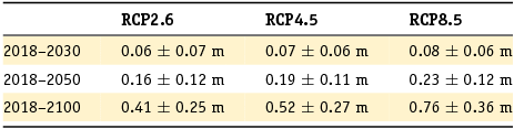
This translates into the following range of rates of sea-level change:
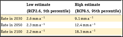
As recent literature suggests a larger projected contribution of the Antarctic ice sheet to sea-level rise than presented in IPCC AR5, we have also assessed the effect of different estimates of accelerated ice mass loss on the total sea-level projections. However, even without the accelerated Antarctic mass loss, the projections for the RCP8.5 scenarios are larger than the high-end projections presented in the 2008 Delta Commission report. Considering the difference in period, the Delta Commission estimate translates to 0.66–0.70m for the 2018–2100 period, compared to 0.76m in this report.
Acknowledgements
We thank three anonymous reviewers for helpful comments and suggestions, NWO for the reviewing process in general and Niels van den Berg and Josef Stuefer in particular, and Willy van Strien for editorial support. The Waddenacademie and Programma naar een Rijke Waddenzee are acknowledged for having initiated and supported this study, notably with financial support for organising a sea-level workshop on 22–23 June 2017 at Royal NIOZ Yerseke.
Appendix: Global mean sea-level change: observations
The palaeo-record
The current position of the coastlines around the world ocean and its shelf seas is, from the perspective of rocks and sediments, the outcome of a long and diverse geological history. From the perspective of water masses and sea surface elevations, however, all these records show a globally common signal. This is due to the world climate having been in glacial–interglacial oscillating mode, as is evident from great amounts of deep sea, shallow marine, and continental biogeochemical, sedimentary and palaeobiological evidence collected and integrated since the 1950s (e.g. Shackleton, Reference Shackleton1969; Lisiecki & Raymo, Reference Lisiecki and Raymo2005; Gibbard & Cohen, Reference Gibbard and Cohen2008), and of which the cyclicity is orbitally forced (e.g. Milankovitch, Reference Milankovitch1941; Imbrie & Imbrie, Reference Imbrie and Imbrie1980; Laskar et al., Reference Laskar, Robutel, Joutel, Gastineau, Correia and Levrard2004).
For the last c.1 million years, in cycles lasting 100,000 years each, the distribution of solar irradiation energy between the atmospheric, oceanic, cryospheric and terrestrial components of the Earth's climate system (e.g. Bintanja et al., Reference Bintanja, van de Wal and Oerlemans2005; Bintanja & Van de Wal, Reference Bintanja and van de Wal2008) has periodically allowed major masses of land ice to build up at higher latitudes on the North American (with a main mass centre on the modern Hudson Bay) and Eurasian continents (main mass centre in the NE of the Baltic Sea). Such withdrawal of water from the oceans pulled down sea levels globally, exposing shallow shelf seas subaerially and allowing terrestrial sedimentary, floral and faunal activity in these areas. At stages of maximum global land-ice mass build up, the sea level in the world ocean stood some 120–150m below where it does today.
Around the world ocean, geological records record sea-level change in various ways. It is seen in the marine oxygen isotope ratio (δ18O) as recorded in coral- and foram carbonates, as well as in the elevations at which shallow water deposition occurred, and in the positions inland on the shelf where one finds deposits of estuaries, lagoons and river mouths. The δ18O signal is such (Broecker & Donk, Reference Broecker and Donk1970; Martinson et al., Reference Martinson, Pisias, Hays, Imbrie, Moore and Shackleton1987) that it allows discrimination between odd-numbered stages of relatively minor Northern Hemisphere ice-sheet water storage, and even-numbered stages with more sizable ice-sheets (Marine Isotope Stages (MIS); e.g. Railsback et al., Reference Railsback, Gibbard, Head, Voarintsoa and Toucanne2015).
The last time that a glacial maximum occurred was between 26,000 and 20,000 years ago (e.g. Peltier & Fairbanks, Reference Peltier and Fairbanks2006; Lambeck et al., Reference Lambeck, Rouby, Purcell, Sun and Sambridge2014). By that time, some 80,000 years into that glacial cycle, the northern hemisphere ice-sheets had extended southward from their northerly inception regions (>65°N) towards temperate latitudes (50–65°N) such as the North American Great Lakes and Europe's North Sea and Polish–German lowlands. Orbital forcing entered a warming limb of its cyclicity and Earth system feedbacks kicked in, helping global climatic amelioration out of the deep glacial maximum and rapidly terminating the ‘glacial’ condition. In some 10,000–15,000 years, a much shorter time than it took to build up the land ice masses, the warmed-up climate made most of the Northern Hemisphere ice storage melt away: only the ice sheet over Greenland remained. Smaller contributions and modest lead–lag times exist between maximum meltwater production from the four main ice-mass centres (Laurentide, Antarctica, Europe, Greenland) during the ‘Termination’ interval.
The termination signal of the last glacial period is recorded in ice-core records on Antarctica and Greenland, in speleothem records at monsoonal tropical and subtropical latitudes, and in terrestrial records of vegetation succession and soil formation. This has offered important cross-validation opportunities for dating the changes and for calibration and validation of geophysical models: for atmospheric climate properties, ocean properties, ice-sheet properties, vegetation cover, river runoff, sediment production – and such models are increasingly combined or interlinked as Earth-system models. The idea is that these models, when calibrated on palaeo-observations and validated, describe Earth-system states from the recent past to the present and the future.
Because GMSL has not fallen since the time of the last major post-glacial sea-level rise (19,000–7000 years ago, peaking at 14,500 years ago), records of post-glacial sea-level rise have remained relatively complete (Carlson & Clark, Reference Carlson and Clark2012; Lambeck et al., Reference Lambeck, Rouby, Purcell, Sun and Sambridge2014). This has made it possible to collect geological data and compile a globally distributed palaeo-observational record of high quality for the post-glacial transgression period (the end of the Last Glacial and first part of the Holocene), as well as for the high-stand period that was the last 7000 years (the rest of the Holocene). Thus, a fair global coverage of palaeo-observational records exists from the last glacial termination (Termination I; MIS2/1 transition). Palaeo-observational records for next older periods are less completely preserved, because, once exposed to sea-level fall, originally submerged and buried records have become terrestrially exposed and subject to various forms of erosion, shrinking the volume. Nevertheless, patches remain in many places around the world, and a globally distributed insight into palaeo-observations of sea-levels for earlier terminations and high stands too (e.g. for the Last Interglacial/Termination II, MIS6/5 transition; Dutton et al., Reference Dutton, Carlson, Long, Milne, Clark, DeConto, Horton, Rahmstorf and Raymo2015). Having such globally distributed insights over multiple glacial–interglacial cycles is important because it allows resolution of spatial differences in sea-level change, known to affect the water surfaces regionally and locally (see earlier sections).
Changes of land surface owing to vertical movement (uplift, subsidence, warping) or sedimentation and erosion complicate the use of palaeo-observations. Good quality palaeo-observations are those that depict a sea-level position 1000–10,000 years ago with dm accuracy, which is dated to 25–100 years accurate (14C dating with some scrutiny can reach this) and is part of a vertical series of data points from a small region so that cross-validation is possible. Fair quality observations indicate the palaeo-sea level to within 1–5m. Opportunities and problems vary between climatic zones (coastal reefs restricted to tropics/subtropics), type of coast (cliffs, mudflats, mangroves, beaches, deltaic, estuarine, lagoonal), distance to past ice sheets (deglaciated, near field, far-field), position to modern coastline (offshore, onshore), position to open ocean (exposed, protected), range of tides, and length of research history (e.g. Van de Plassche, Reference Van de Plassche1986; Shennan et al., Reference Shennan, Long and Horton2015).
The tide-gauge record
Tide-gauge instruments have been measuring sea level for the last few centuries. The world's oldest written sea-level record is from a tide gauge at Amsterdam, in place since the year 1700 (Van Veen, Reference Van Veen1954). From the mid-19th century onwards, multiple tide-gauge records are available, from places spread over the world. Tide gauges are primarily installed to monitor the local tidal regime at ports to facilitate shipping, but have also been used to study long-term sea-level change. Such applications require, however, a careful logging of on-site local datum shifts, and instrument changes, which are not always available.
The Permanent Service for Mean Sea Level (PSMSL) has a large collection of quality checked tide-gauge records all over the world, but does not contain all existing records (Hogarth, Reference Hogarth2014). The tide-gauge records have been used to estimate GMSL changes. Since sea-level changes differ from place to place, reconstructing GMSL changes from the limited set of tide-gauge records remains challenging. The number of available tide gauge records varies strongly over time: in the beginning of the record (1860s) only 7–14 tide gauge records are available, while over the last few decades hundreds of records are available. Furthermore, most of the longer records are only available from the Northern Hemisphere, in particular from the European and North American coastlines. Multiple techniques and corrections have been proposed to better reconstruct GMSL, although this topic is still under active debate. The sparse sampling of tide gauges in the early part of the record, leads to larger uncertainties especially before 1960 (e.g. Church & White, Reference Church and White2011; Jevrejeva et al., Reference Jevrejeva, Moore, Grinsted, Matthews and Spada2014; Slangen et al., Reference Slangen, Church, Agosta, Fettweis, Marzeion and Richter2016; Dangendorf et al., Reference Dangendorf, Marcos, Wöppelmann, Conrad, Frederikse and Riva2017). Recent reconstructions try to better reflect errors introduced by the sampling, and better account for local sea-level effects as induced by the non-uniform response of sea level from glaciers and ice sheets (Hay et al., Reference Hay, Morrow, Kopp and Mitrovica2015; Thompson et al., Reference Thompson, Hamlington, Landerer and Adhikari2016; Dangendorf et al., Reference Dangendorf, Marcos, Wöppelmann, Conrad, Frederikse and Riva2017).
In general, tide-gauge based reconstruction studies agree that sea level over the 20th century has risen by c.11–18cm, and that the rate of sea-level rise is accelerating (Fig. A1), although the magnitude of the total change and of the acceleration varies significantly between individual reconstructions. The Jevrejeva et al. (Reference Jevrejeva, Moore, Grinsted and Woodworth2008) sea-level reconstruction from 1700 to 2003 indicates an acceleration of 0.01mma−2. Similarly, Church & White (Reference Church and White2011) found 1.7±0.4mma−1 sea-level rise over the period 1880 to 2009, with a significant acceleration of 0.009±0.003mma−2. Hay et al. (Reference Hay, Morrow, Kopp and Mitrovica2015) introduced two probabilistic reconstruction approaches, which both resulted in an overall lower trend of 1.3±0.2mma−1 (1901–2010), and a stronger acceleration of 0.017±0.003mma−2. These were confirmed by Dangendorf et al. (Reference Dangendorf, Marcos, Wöppelmann, Conrad, Frederikse and Riva2017), who developed and applied an area-weighting approach and corrections for local vertical land motion. With that method, they found a trend of 1.3±0.2mma−1 over the years 1902–2012, and an associated acceleration of 0.018±0.008mma−2.
Global Mean Sea Level (GMSL) reconstructions based on tide gauges using different reconstruction techniques compared to climate model results. First three reconstructions from Dangendorf et al. (Reference Dangendorf, Marcos, Wöppelmann, Conrad, Frederikse and Riva2017) (black, black dash, red). Mean of three reconstructions (CW11 Church & White (Reference Church and White2011), RD11 Ray & Douglas (Reference Ray and Douglas2011), J14 Jevrejeva et al. (Reference Jevrejeva, Moore, Grinsted, Matthews and Spada2014)) (yellow). Reconstruction H15 from Hay et al. (Reference Hay, Morrow, Kopp and Mitrovica2015). Individual climate model results (light blue) and model ensemble (dark blue) from Slangen et al. (Reference Slangen, Meyssignac, Agosta, Champollion, Church, Fettweis, Ligtenberg, Marzeion, Melet, Palmer, Richter, Roberts and Spada2017a). Figure from Dangendorf et al. (Reference Dangendorf, Marcos, Wöppelmann, Conrad, Frederikse and Riva2017).
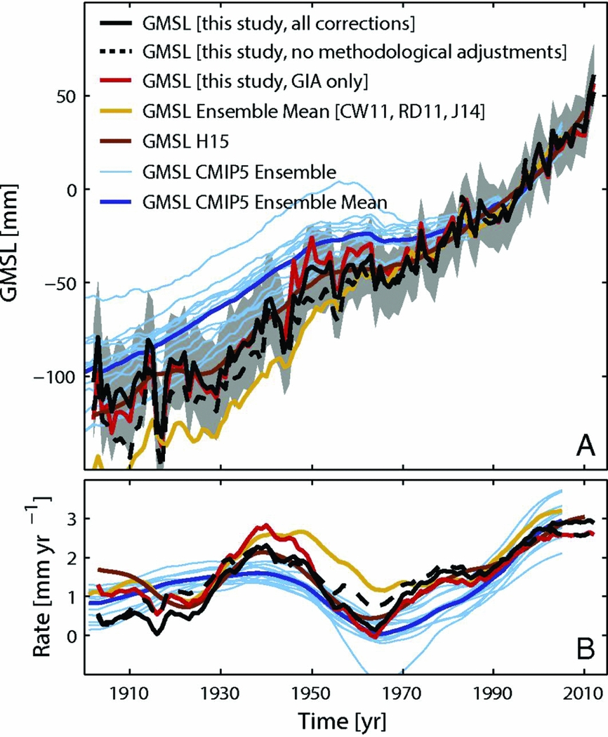
The satellite era
In the satellite era, geocentric sea level, ocean mass and steric sea level can be observed separately using independent observation systems. Geocentric sea level is observed with satellite radar altimeters. It uses the two-way travel time of a radar pulse to estimate the range between the satellite and the earth's surface, which are then converted to a height above a reference ellipsoid by using the precisely determined orbits of the altimeters. Variations in the mass component are derived from gravity fields estimated from the GRACE twin satellites, which have been in orbit since 2002. The steric sea level is estimated from temperature and salinity (T/S) measurements, which are primarily obtained from instruments deployed from ships and an autonomous system of Argo floats.
Satellite radar altimetry
The high-quality radar altimeter record that allows us to quantify long-term sea level variations started with the launch of the TOPEX/Poseidon satellite in 1992. The satellite was launched in a 66° inclination, 10-day repeat orbit, which causes an equatorial ground-track spacing of c.315km (along-track sampling spacing is c.300m, but often averaged over 6–7km in large databases). TOPEX/Poseidon was succeeded by the Jason-1, -2 and -3 missions, resulting in a continuous record till now.
Apart from this, long-term sea-level variations can be derived from the radar altimeters on board several European Earth observation satellites (ERS-1, ERS-2, Envisat) and the dedicated SARAL/AltiKa altimetry satellite mission. During their nominal mission phase, these satellite orbits have an 82° inclination, and a 35-day ground-track repeat period. Hence, they cover a larger part of the world's oceans, such as the high-latitude Arctic. Compared to the TOPEX/Poseidon – Jason series, the data acquired by these satellites provide a higher spatial resolution; the equatorial ground-track spacing is c.80km. Note that there is a data gap of c.1 year between the Envisat and the SARAL missions (in 2012–13). The data acquired by the other satellite radar altimeter missions (Sentinel-3, Cryosat-2, HY-2A and GeoSat Follow-On) are generally not yet used to monitor long-term sea-level variations.
Regular estimates of the GMSL variations are produced by five research groups, including the University of Colorado (CU; Nerem et al., Reference Nerem, Chambers, Choe and Mitchum2010), Goddard Space Flight Center (GSFC; Beckley et al., Reference Beckley, Zelensky, Holmes, Lemoine, Ray, Mitchum, Desai and Brown2010), the US National Oceanic and Atmospheric Administration (NOAA; Leuliette & Scharroo, Reference Leuliette and Scharroo2010), LEGOS/CNES/CLS (AVISO; Ablain et al., Reference Ablain, Cazenave, Valladeau and Guinehut2009), and CSIRO (Church & White, Reference Church and White2011). Apart from AVISO, no group includes the data acquired by the ERS-1, ERS-2, Envisat and SARAL/AltiKa satellites. All GMSL time series reveal significant interannual variability; in particular, the larger El Niño (1998, 2015) and the La Niña events (2011) are detectable (Boening et al., Reference Boening, Willis, Landerer, Nerem and Fasullo2012; Cazenave et al., Reference Cazenave, Henry, Munier, Delcroix, Gordon, Meyssignac, Llovel, Palanisamy and Becker2012). Due to different processing methods, the time series differ at monthly to interannual timescales (Masters et al., Reference Masters, Nerem, Choe, Leuliette, Beckley, White and Ablain2012). The obtained trends are, however, statistically equal: c.3.3±0.4mma−1 over the period 1993–2016. This trend includes a correction for GIA of 0.3mma−1 (e.g. Nerem et al., Reference Nerem, Chambers, Choe and Mitchum2010), which is due to the mean subsidence of the ocean floor.
Though the estimated trends presented by the five research groups are statistically equal, they might all be contaminated by systematic errors and hence deviate from the actual trend in GMSL. The stability of the GMSL record is monitored by a comparison to in situ tide gauge measurements (Mitchum, Reference Mitchum1998, Reference Mitchum2000). An in-depth comparison with tide gauges corrected for vertical land motion revealed a significant drift in the TOPEX/Poseidon phase A (Watson et al., Reference Watson, White, Church, King, Burgette and Legresy2015), which is probably related to the internal path delay calibration of the instrument. After accounting for this drift, the GMSL trend drops by c.0.4mma−1 (Watson et al., Reference Watson, White, Church, King, Burgette and Legresy2015).
A second source of systematic error might be introduced by omission of the polar regions (Henry et al., Reference Henry, Ablain, Meyssignac, Cazenave, Masters, Nerem and Garric2014). GMSL trends estimated from the TOPEX/Poseidon – Jason series only include observations below 66° latitude. In a recent study, Carret et al. (Reference Carret, Johannessen, Andersen, Ablain, Prandi, Blazquez and Cazenave2017) estimated a trend of 2.10±0.63mma−1 over the period 1992 to 2014 for the high-latitude and Arctic Ocean (66–80°N) based on data from the ERS-1/2, Envisat and Cryosat-2 altimeter missions. As their estimate is lower than the GMSL trend, it suggests that the GMSL trends are probably too high. At the same time, the bias might be well within the error bars of the GMSL trend given the fact that the considered oceanic area is small.
Recent studies showed that there is likely a positive acceleration in the altimeter-derived GMSL time series (Watson et al., Reference Watson, White, Church, King, Burgette and Legresy2015; Fasullo et al., Reference Fasullo, Nerem and Hamlington2016). Previously, such an acceleration had not been detectable (Cazenave et al., Reference Cazenave, Dieng, Meyssignac, von Schuckmann, Decharme and Berthier2014), which can be attributed to (i) the aforementioned drift in the TOPEX phase A record (Watson et al., Reference Watson, White, Church, King, Burgette and Legresy2015; Chen et al., Reference Chen, Zhang, Church, Watson, King, Monselesan, Legresy and Harig2017), and (ii) the recovery from a dip in global ocean heat content at the beginning of the altimeter record due to the eruption of Mount Pinatubo in 1991 (Fasullo et al., Reference Fasullo, Nerem and Hamlington2016).
Global Ocean Mass changes from satellite gravimetry
Most Global Ocean Mass (GOM) time series are derived from the official GRACE-based (Tapley et al., Reference Tapley, Bettadpur, Watkins and Reigber2004) gravity field solutions produced by either NASA's Jet Propulsion Laboratory (JPL), the German Research Center for Geosciences (GFZ) or the Center for Space Research (CSR) of the University of Texas. These solutions are provided as sets of monthly mean Stokes coefficients and are available over the period 2002–17. As the GRACE solutions are provided in the instantaneous centre of common mass frame, so-called ‘geocentre motion’ corrections need to be applied to compute GOM variations. These corrections can be indirectly inferred from GRACE data and geophysical models (Swenson et al., Reference Swenson, Chambers and Wahr2008; Sun et al., Reference Sun, Ditmar and Riva2017) or can be computed from terrestrial network deformations derived from Global Navigation Satellite Systems (GNSS) and/or satellite laser ranging data (Collilieux et al., Reference Collilieux, Altamimi, Ray, van Dam and Wu2009; Rietbroek et al., Reference Rietbroek, Fritsche, Brunnabend, Daras, Kusche, Schröter, Flechtner and Dietrich2012a; Riddell et al., Reference Riddell, King, Watson, Sun, Riva and Rietbroek2017). Additionally, the poorly constrained C20 spherical harmonic coefficient representing the variation in the Earth's oblateness is often replaced by an estimate from satellite laser ranging (Cheng et al., Reference Cheng, Tapley and Ries2013).
Chambers et al. (Reference Chambers, Cazenave, Champollion, Dieng, Llovel, Forsberg, von Schuckmann and Wada2017) estimated a GOM sea-level equivalent trend of 2.1±0.4mma−1 over the period 2005–15 from the three official GRACE-based gravity field solutions. These ocean mean mass time series were also used to compute trends of the GOM component in Dieng et al. (Reference Dieng, Cazenave, Meyssignac and Ablain2017) and Piecuch & Quinn (Reference Piecuch and Quinn2016). The latter provided a GOM sea-level equivalent trend of 2.2±0.4mma−1 over the period 2005–16, while including the Multivariate ENSO Index (MEI) in the regression, arguing that about half of the interannual sea level due to El Niño–Southern Oscillation (ENSO) is associated with GOM variations. The estimated GOM trend based on the JPL mascon solution (Watkins et al., Reference Watkins, Wiese, Yuan, Boening and Landerer2015) is slightly smaller: 1.8±0.2mma−1 sea-level equivalent over the period 2002.5–2016.5. By using an iterative method applied to GRACE data, Chen et al. (Reference Chen, Wilson and Tapley2013) estimated a larger rate of 2.39±0.48mma−1 over the shorter period (2005–2011). Based on a joint inversion of radar altimetry and GRACE data, Rietbroek et al. (Reference Rietbroek, Brunnabend, Kusche, Schröter and Dahle2016) found a lower GOM trend of 1.08±0.3mma−1 sea-level equivalent over the period 2002–14.
Several problems exist that may introduce biases or limit the usability of the GRACE-based GOM trend estimates. First, in the first two years of the GRACE mission and after 2012 there are many gaps in the GRACE data record. Moreover, there is a degraded performance of GRACE associated with technical problems and operational decisions such as the switching-off of instruments for battery saving (Flechtner et al., Reference Flechtner, Neumayer, Dahle, Dobslaw, Fagiolini, Raimondo and Güntner2016). Additionally, the quality of the GRACE monthly mean gravity field solutions is lower in several periods due to data gaps (since 2011; see Flechtner et al., Reference Flechtner, Morton, Watkins, Webb and Marti2014) or unfavourable orbit sampling (Wagner et al., Reference Wagner, McAdoo, Klokočník and Kostelecký2006). Second, the spatial resolution of GRACE is c.250–300km, which makes GOM variation estimates prone to leakage from land hydrology signals into the ocean. To mitigate leakage, often all grid points within 300km of the coasts are excluded. As shown by Kleinherenbrink et al. (Reference Kleinherenbrink, Riva and Sun2016), however, this introduces small biases. Finally, GRACE-based GOM estimates do not include the effects of Earth rotation. This primarily affects the spherical harmonic components C21 and S21, related to polar motion. Wahr et al. (Reference Wahr, Nerem and Bettadpur2015) argued that the full polar motion (C21/S21) signal should be removed, except for the trend in it caused by GIA. In doing so, part of the ocean mass is removed. On the other hand, the GRACE-based GOM estimates become more consistent to altimetry.
Temperature and salinity observations
Steric sea-level changes, i.e. changes due to variations in sea water density, are inferred from salinity and temperature measurements. Together with the ocean mass changes, they contribute to sea level change.
Before 2000, observational estimates of steric sea-level change relied mainly on sporadic shipboard measurements using Expendable BathyThermograph (XBT) or Conductivity, Temperature, Depth (CTD) devices. The largest fraction of the observations originates from XBTs. These rely on fall velocities calibrated in a laboratory, which might induce time-variable biases in the estimated temperature profiles (Gouretski & Koltermann, Reference Gouretski and Koltermann2007). In current databases these biases are typically corrected for by a comparison with the CTDs. Even though biases in fall speed are corrected for, substantial biases still occur due to inhomogeneous sampling: the northern hemisphere is substantially better sampled than the southern hemisphere, but nevertheless contains large gaps. This makes gridded T/S data products such as the World Ocean Atlas (Locarnini et al., Reference Locarnini, Mishonov, Antonov, Boyer, Garcia, Baranova, Zweng, Paver, Reagan, Johnson, Hamilton and Seidov2013) less accurate in the undersampled parts of the ocean.
Since 2000, Argo floats have been deployed, which sample the ocean T/S up to 2000m depth every 10 days. The Argo programme was designed to recover temperature and salinity variations beyond mesoscale, which required one float per 3 × 3° box, i.e. c.3000 floats (Roemmich & Gilson, Reference Roemmich and Gilson2009; Leuliette & Willis, Reference Leuliette and Willis2011). This objective was achieved in November 2007 (Leuliette & Willis, Reference Leuliette and Willis2011). Estimates of steric height based on Argo data are typically made from 2004 to 2005, when a significant number of observations are present (Cabanes et al., Reference Cabanes, Grouazel, von Schuckmann, Hamon, Turpin, Coatanoan, Paris, Guinehut, Boone, Ferry, de Boyer Montégut, Carval, Reverdin, Pouliquen and Le Traon2013). Most of the gridded data products are based on data from all types of T/S measurements. This applies to the commonly used EN4 (Good et al., Reference Good, Martin and Rayner2013) and Ishii & Kimoto (Reference Ishii and Kimoto2009) datasets. The data products from the Japan Agency for Marine–Earth Science and Technology (JAMSTEC) (Hosoda et al., Reference Hosoda, Ohira and Nakamura2008) and Scripps (Roemmich & Gilson, Reference Roemmich and Gilson2009) are, however, solely based on Argo data. Another type of gridded T/S data product is obtained from ocean reanalyses. Here, in situ T/S observations, altimetry data and sea surface temperature measurements are assimilated into an ocean model (e.g. Balmaseda et al., Reference Balmaseda, Hernandez, Storto, Palmer, Alves, Shi, Smith, Toyoda, Valdivieso, Barnier, Behringer, Boyer, Chang, Chepurin, Ferry, Forget, Fujii, Good, Guinehut, Haines, Ishikawa, Keeley, Köhl, Lee, Martin, Masina, Masuda, Meyssignac, Mogensen, Parent, Peterson, Tang, Yin, Vernieres, Wang, Waters, Wedd, Wang, Xue, Chevallier, Lemieux, Dupont, Kuragano, Kamachi, Awaji, Caltabiano, Wilmer-Becker and Gaillard2015). Note that these models often make use of the Boussinesq approximation (i.e. they conserve volume rather than mass), which introduces mass consistency problems when estimating trends (Greatbatch, Reference Greatbatch1994).
A comparison of steric time series computed from reanalyses and gridded data products by Storto et al. (Reference Storto, Yang and Masina2016) showed significant differences. The steric trends computed over the period 1993–2010 differed between 0 and 3mma−1, with an average of c.1mma−1, which is primarily a thermosteric effect. The spread between the products is significantly larger before 1998. Several studies computed trends over the Argo period. The trends appeared to be unchanged with respect to the 1993–2010 period, with estimates of 0.8±0.2mma−1 over 2004–2015.5 (Llovel et al., Reference Llovel, Willis, Landerer and Fukumori2014), 1.0±0.5mma−1 over 2005–2013 (Leuliette, Reference Leuliette2015), and 1.0±0.2mma−1 over 2005–2016 (Piecuch & Quinn, Reference Piecuch and Quinn2016). Piecuch & Quinn (Reference Piecuch and Quinn2016) also demonstrated that approximately half of the GMSL variability is explained by the steric water level variations.
There are several systematic error sources that can bias the estimated steric trends. First, steric sea level in ice-covered polar waters cannot be properly determined from grids produced by statistically optimal interpolation. Since most GMSL time series also include radar altimeter observations up to 66° latitude only (see above), the polar waters are often omitted. According to Andersen & Piccioni (Reference Andersen and Piccioni2016), the trend in mean steric sea level is statistically insignificant after 2005, while another study estimated a positive trend of c.1mma−1 between 2003 and 2010 (Carret et al., Reference Carret, Johannessen, Andersen, Ablain, Prandi, Blazquez and Cazenave2017), comparable to the global average. The omission of the polar waters will therefore not cause a significant bias on the steric trend estimates over the considered period.
A second bias in steric sea level could be introduced by warming of the deep ocean, which is not sampled by Argo even though the newest floats reach a depth of 4000m. Several studies investigated the possibility of deep ocean warming, but the effect on global mean steric change appeared to be insignificant (Llovel et al., Reference Llovel, Willis, Landerer and Fukumori2014; Von Schuckmann et al., Reference Von Schuckmann, Sallée, Chambers, Le Traon, Cabanes, Gaillard, Speich and Hamon2014). However, it might be significant on a local scale (Von Schuckmann et al., Reference Von Schuckmann, Sallée, Chambers, Le Traon, Cabanes, Gaillard, Speich and Hamon2014; Volkov et al., Reference Volkov, Lee, Landerer and Lumpkin2017). Albeit sparse, measurements in the deep ocean (below 4000m) indicated trends of 0.053±0.017mma−1 augmented by an additional contribution of 0.093±0.081mma−1 from the Southern Ocean between 1000 and 4000m depth (Purkey & Johnson, Reference Purkey and Johnson2010). A study based on hydrographic measurements also indicated a trend of 0.095mma−1 for depths below 3000m (Kouketsu et al., Reference Kouketsu, Doi, Kawano, Masuda, Sugiura, Sasaki, Toyoda, Igarashi, Kawai, Katsumata, Uchida, Fukasawa and Awaji2011). Finally, the continental shelves and several small sea basins are not sampled by Argo. The most important area that introduces biases is the Tropical Asian Seas (Von Schuckmann et al., Reference Von Schuckmann, Sallée, Chambers, Le Traon, Cabanes, Gaillard, Speich and Hamon2014). To get an estimate of the steric sea level change due to temperature and salinity in these waters, reanalysis data is used. Dieng et al. (Reference Dieng, Cazenave, Meyssignac and Ablain2017) and Kleinherenbrink et al. (Reference Kleinherenbrink, Riva, Frederikse, Merrifield and Wada2017) showed that the omission of these waters results in trends that are 0.2–0.3mma−1 too low.
Global mean sea-level budget
The intercomparison between mass-driven sea level from gravimetry, steric sea level from models or temperature and salinity data, and total (geocentric) sea level as measured by radar altimetry, allows the closure of the sea-level budget (Leuliette, Reference Leuliette2015). For example, using radar altimetry with gravimetry allows the retrieval of the steric sea level component which can then be validated using independent estimates from models and/or observations. The GMSL consists of mass contributions and a steric contribution, but a finer delineation is also possible.
In the IPCC AR5 report (Church et al., Reference Church, Clark, Cazenave, Gregory, Jevrejeva, Levermann, Merrifield, Milne, Nerem, Nunn, Payne, Pfeffer, Stammer, Unnikrishnan, Stocker, Qin, Plattner, Tignor, Allen, Boschung, Nauels, Xia, Bex and Midgley2013), the contributions to the GMSL budget from both modelling and observational sources have been tabulated (their table 13.1) for the time periods 1901–90, 1971–2010 and 1993–2010 (satellite era). From both models and observations it is clear that thermosteric sea level rise and the contributions from glaciers and ice sheets have been increasing over the years. A more up-to-date GMSL budget over the satellite era is provided in Table A1 (Chambers et al., Reference Chambers, Cazenave, Champollion, Dieng, Llovel, Forsberg, von Schuckmann and Wada2017, their table 1).
Estimated trends in global mean sea level and components for the period 1993–2015 (table 1 from Chambers et al., Reference Chambers, Cazenave, Champollion, Dieng, Llovel, Forsberg, von Schuckmann and Wada2017). Exact time period for each representative time series is given. Uncertainty is 90% confidence, except for the thermosteric below 2000m, which is 95% as estimated by Purkey & Johnson (Reference Purkey and Johnson2010).
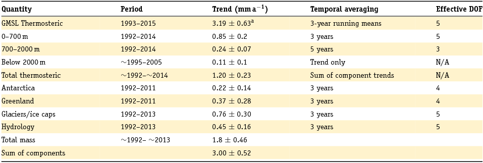
Although the GMSL budget can now be closed within uncertainties (e.g. Gregory et al., Reference Gregory, White, Church, Bierkens, Box, van den Broeke, Cogley, Fettweis, Hanna, Huybrechts, Konikow, Leclercq, Marzeion, Oerlemans, Tamisiea, Wada, Wake and van de Wal2013), the estimates of different contributions produced by various research groups can still show appreciable differences, depending on the time period considered and the data origin. Von Schuckmann et al. (Reference Von Schuckmann, Sallée, Chambers, Le Traon, Cabanes, Gaillard, Speich and Hamon2014) assessed the GMSL budget using Argo measurements, GRACE gravimetry and radar altimetry. They warned that an incomplete sampling for Argo (especially in the region around the tropical Asian Archipelago) may be one of the reasons for biases in steric sea level variations.
Recently, the use of joint inversion methods which allow a direct estimation of the GMSL budget components from GRACE and radar altimetry have been discussed (Rietbroek et al., Reference Rietbroek, Brunnabend, Kusche and Schröter2012b, Reference Rietbroek, Brunnabend, Kusche, Schröter and Dahle2016). These methods use the full error-covariance information from the observations and differ in the way that the sea-level contributions are parameterised. In contrast to using spherical harmonic coefficients, patterns of (non-uniform) sea level changes are prescribed for several contributors (i.e. sea-level response to changes of glaciers, ice sheet, terrestrial hydrology, GIA and steric sea-level changes), whose time variations are then solved for in a single adjustment. Using a joint inversion method, Rietbroek et al. (Reference Rietbroek, Brunnabend, Kusche, Schröter and Dahle2016) found a GMSL trend of 2.74±0.58mma−1 over the period 2002–14, which was explained by a relatively large steric sea level contribution of 1.38±0.16mma−1 and a relatively low mass contribution of 1.08±0.09mma−1 (1.37 ±0.09mma−1 excluding hydrology) (Fig. A2).
Global mean relative sea level, divided into different contributions. Annual and semiannual harmonics have been fitted and removed and the resulting curves are smoothed with a 3-month running mean (trends are derived from the unsmoothed data). The curves have been offset for clarity. The component denoted ‘other’ reflects large-scale sea-level signals in altimetry that are not explained by the other contributions (Rietbroek et al., Reference Rietbroek, Brunnabend, Kusche, Schröter and Dahle2016). Figure from Rietbroek et al. (Reference Rietbroek, Brunnabend, Kusche, Schröter and Dahle2016, fig. 1).
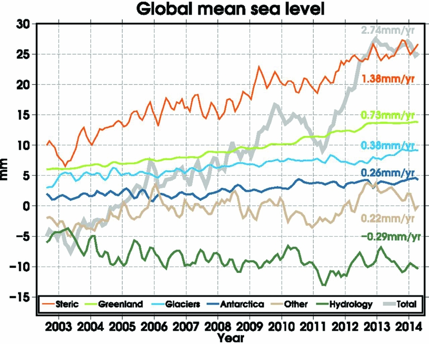


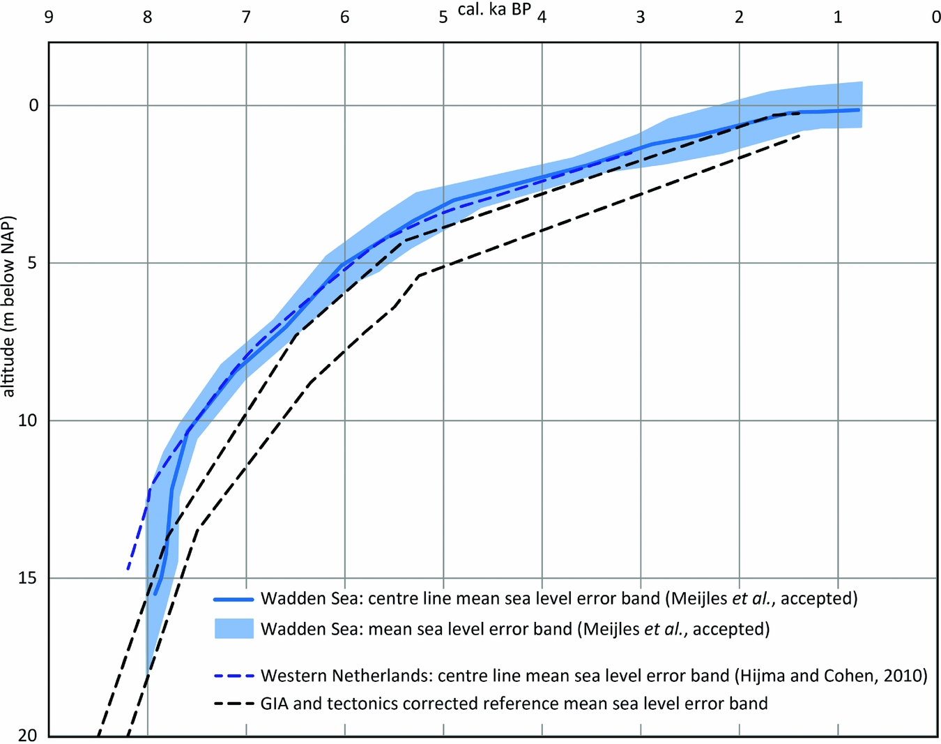


 Open access