

1 Introduction
Elliptic K3 surfaces play an important role in the study of the geometry, arithmetic and moduli of K3 surfaces [Reference Piatetski-Shapiro and ShafarevichP-SS, Reference Shioda and InoseSI, Reference Artin and Swinnerton-DyerAS-D, Reference MorrisonMo, Reference Bogomolov and TschinkelBT].
An elliptic surface
 ${\mathcal{E}}$
fibered over
${\mathcal{E}}$
fibered over
 $\mathbb{P}^{1}$
with section, over a field
$\mathbb{P}^{1}$
with section, over a field
 $k$
, may be described by a Weierstrass equation of the form
$k$
, may be described by a Weierstrass equation of the form
 $$\begin{eqnarray}y^{2}+a_{1}(t)xy+a_{3}(t)y=x^{3}+a_{2}(t)x^{2}+a_{4}(t)x+a_{6}(t),\end{eqnarray}$$
where the
 $a_{i}(t)$
are rational functions (or even polynomials). Let us assume that the elliptic fibration has at least one singular fiber. The following is a fundamental question:
$a_{i}(t)$
are rational functions (or even polynomials). Let us assume that the elliptic fibration has at least one singular fiber. The following is a fundamental question:
Question 1.1. Find generators for the (finitely generated) Mordell–Weil group
 ${\mathcal{E}}(\mathbb{P}^{1})$
.
${\mathcal{E}}(\mathbb{P}^{1})$
.
Usually, one is interested in the geometric Mordell–Weil group
 ${\mathcal{E}}(\overline{k}(t))$
, as well as its field of definition and the Galois action of
${\mathcal{E}}(\overline{k}(t))$
, as well as its field of definition and the Galois action of
 $\operatorname{Gal}(\overline{k}/k)$
.
$\operatorname{Gal}(\overline{k}/k)$
.
A theorem of Shioda and Tate connects the Mordell–Weil group with the Picard group or the Néron–Severi group of
 ${\mathcal{E}}$
(note that linear equivalence and algebraic equivalence coincide). Namely, there is an intersection pairing on
${\mathcal{E}}$
(note that linear equivalence and algebraic equivalence coincide). Namely, there is an intersection pairing on
 $\operatorname{NS}({\mathcal{E}})$
, making it into a Lorentzian lattice. The class of the zero section
$\operatorname{NS}({\mathcal{E}})$
, making it into a Lorentzian lattice. The class of the zero section
 $O$
and the fiber
$O$
and the fiber
 $F$
contribute a unimodular sublattice of signature
$F$
contribute a unimodular sublattice of signature
 $(1,1)$
, which is therefore either the hyperbolic plane
$(1,1)$
, which is therefore either the hyperbolic plane
 $U$
or the odd lattice
$U$
or the odd lattice
 $\text{I}_{1,1}=\langle 1\rangle \oplus \langle -1\rangle$
, depending on the Euler characteristic
$\text{I}_{1,1}=\langle 1\rangle \oplus \langle -1\rangle$
, depending on the Euler characteristic
 $\unicode[STIX]{x1D712}({\mathcal{O}}_{{\mathcal{E}}})$
. Furthermore, every reducible fiber over a point
$\unicode[STIX]{x1D712}({\mathcal{O}}_{{\mathcal{E}}})$
. Furthermore, every reducible fiber over a point
 $v\in \mathbb{P}^{1}(\overline{k})$
contributes the negative of a root lattice
$v\in \mathbb{P}^{1}(\overline{k})$
contributes the negative of a root lattice
 $T_{v}$
to
$T_{v}$
to
 $\operatorname{NS}({\mathcal{E}})$
. Let the trivial lattice
$\operatorname{NS}({\mathcal{E}})$
. Let the trivial lattice
 $T$
be defined as
$T$
be defined as
 $(\mathbb{Z}O+\mathbb{Z}F)\oplus (\bigoplus T_{v})$
. The theorem says that the Mordell–Weil group
$(\mathbb{Z}O+\mathbb{Z}F)\oplus (\bigoplus T_{v})$
. The theorem says that the Mordell–Weil group
 ${\mathcal{E}}(\mathbb{P}^{1})$
is isomorphic to
${\mathcal{E}}(\mathbb{P}^{1})$
is isomorphic to
 $NS({\mathcal{E}})/T$
. In addition, the natural isomorphism induces an isometry of lattices, once we mod out by torsion.
$NS({\mathcal{E}})/T$
. In addition, the natural isomorphism induces an isometry of lattices, once we mod out by torsion.
It guarantees that determination of the Mordell–Weil group is equivalent to finding the Picard group or the Néron–Severi lattice of the K3 surface. The theory of Mordell–Weil lattices has found numerous applications in recent years, from construction of record-breaking dense lattices to finding high rank elliptic curves to the inverse Galois problem.
Recently, algorithms have been outlined for the basic question above (see [Reference Poonen, Testa and van LuijkPTvL], or for the case of elliptic K3 surfaces [Reference CharlesCh]); however, these algorithms require point counting over large finite fields, and therefore are not practicable in most cases.
In this paper, we solve this question for several families of K3 surfaces of arithmetic and geometric interest. Namely, let
 $E_{1}$
and
$E_{1}$
and
 $E_{2}$
be two elliptic curves, and form the Kummer surface of their product
$E_{2}$
be two elliptic curves, and form the Kummer surface of their product
 $\mathit{Km}(E_{1}\times E_{2})$
. This K3 surface carries a lot of the arithmetic information of the product abelian surface. It has several different elliptic fibrations [Reference OguisoO, Reference Kuwata and ShiodaKS], but one in particular has been the focus of a lot of attention in arithmetic algebraic geometry. This elliptic fibration (to be described below) has two reducible fibers of type
$\mathit{Km}(E_{1}\times E_{2})$
. This K3 surface carries a lot of the arithmetic information of the product abelian surface. It has several different elliptic fibrations [Reference OguisoO, Reference Kuwata and ShiodaKS], but one in particular has been the focus of a lot of attention in arithmetic algebraic geometry. This elliptic fibration (to be described below) has two reducible fibers of type
 $\text{IV}^{\ast }$
if
$\text{IV}^{\ast }$
if
 $E_{1}$
and
$E_{1}$
and
 $E_{2}$
are non-isomorphic. By taking a base change along an appropriate double cover
$E_{2}$
are non-isomorphic. By taking a base change along an appropriate double cover
 $\mathbb{P}^{1}\rightarrow \mathbb{P}^{1}$
(namely
$\mathbb{P}^{1}\rightarrow \mathbb{P}^{1}$
(namely
 $t\mapsto t^{2}$
, where
$t\mapsto t^{2}$
, where
 $t$
is the elliptic parameter, chosen to place the
$t$
is the elliptic parameter, chosen to place the
 $\text{IV}^{\ast }$
fibers at
$\text{IV}^{\ast }$
fibers at
 $t=0$
and
$t=0$
and
 $t=\infty$
), a natural double cover of the Kummer surface can be formed, which is also an elliptic K3 surface; it is called the Inose surface and has been useful in several contexts [Reference Shioda and InoseSI, Reference InoseI2, Reference KumarKm, Reference ElkiesE, Reference ShiodaSh4]. In [Reference KuwataKw2], Masato Kuwata defined elliptic K3 surfaces
$t=\infty$
), a natural double cover of the Kummer surface can be formed, which is also an elliptic K3 surface; it is called the Inose surface and has been useful in several contexts [Reference Shioda and InoseSI, Reference InoseI2, Reference KumarKm, Reference ElkiesE, Reference ShiodaSh4]. In [Reference KuwataKw2], Masato Kuwata defined elliptic K3 surfaces
 $F^{(1)}$
through
$F^{(1)}$
through
 $F^{(6)}$
through a base change of the Inose surface, and used them to produce elliptic K3 surfaces over
$F^{(6)}$
through a base change of the Inose surface, and used them to produce elliptic K3 surfaces over
 $\mathbb{Q}$
of every geometric rank between
$\mathbb{Q}$
of every geometric rank between
 $1$
and
$1$
and
 $18$
, except for
$18$
, except for
 $15$
. (The rank
$15$
. (The rank
 $15$
case was dealt with several years later by Kloosterman [Reference KloostermanKl1]. See also [Reference Top and de ZeeuwTdZ] for an extension, and the note [Reference Kumar and KuwataKK] which provides a construction starting from a Kummer surface.) In particular,
$15$
case was dealt with several years later by Kloosterman [Reference KloostermanKl1]. See also [Reference Top and de ZeeuwTdZ] for an extension, and the note [Reference Kumar and KuwataKK] which provides a construction starting from a Kummer surface.) In particular,
 $F^{(1)}$
is the Inose surface, and
$F^{(1)}$
is the Inose surface, and
 $F^{(2)}$
is the Kummer surface.
$F^{(2)}$
is the Kummer surface.
The main purpose of this article is to describe completely explicitly the Mordell–Weil lattices of these elliptic K3 surfaces
 $F_{E_{1}\times E_{2}}^{(n)}$
in the “generic” caseFootnote
1
, that is, when
$F_{E_{1}\times E_{2}}^{(n)}$
in the “generic” caseFootnote
1
, that is, when
 $E_{1}$
and
$E_{1}$
and
 $E_{2}$
are not isogenous. As a result, we also recover by specialization a finite index sublattice of the full Mordell–Weil lattice in the nongeneric case. We will show that the splitting field in the generic case is a subfield of the compositum
$E_{2}$
are not isogenous. As a result, we also recover by specialization a finite index sublattice of the full Mordell–Weil lattice in the nongeneric case. We will show that the splitting field in the generic case is a subfield of the compositum
 $\unicode[STIX]{x1D705}_{n}:=k(E_{1}[n],E_{2}[n])$
of the
$\unicode[STIX]{x1D705}_{n}:=k(E_{1}[n],E_{2}[n])$
of the
 $n$
-torsion subfields of the two elliptic curves, where
$n$
-torsion subfields of the two elliptic curves, where
 $k$
is the base field, and use natural group actions of
$k$
is the base field, and use natural group actions of
 $\operatorname{GL}_{2}(\mathbb{Z}/n\mathbb{Z})^{2}$
on the universal family of
$\operatorname{GL}_{2}(\mathbb{Z}/n\mathbb{Z})^{2}$
on the universal family of
 $F^{(n)}$
over pairs of elliptic curves with level
$F^{(n)}$
over pairs of elliptic curves with level
 $n$
structure to give relatively concise descriptions of explicit bases for the Mordell–Weil lattices.
$n$
structure to give relatively concise descriptions of explicit bases for the Mordell–Weil lattices.
The last part of this paper is arithmetic and describes the Mordell–Weil lattices of
 $F_{E_{1}\times E_{2}}^{(n)}$
, for those pairs of elliptic curves such that the Inose surface
$F_{E_{1}\times E_{2}}^{(n)}$
, for those pairs of elliptic curves such that the Inose surface
 $F^{(1)}$
is defined over
$F^{(1)}$
is defined over
 $\mathbb{Q}$
and is singular, that is, has the maximal Picard number
$\mathbb{Q}$
and is singular, that is, has the maximal Picard number
 $20$
. In this case,
$20$
. In this case,
 $E_{1}$
and
$E_{1}$
and
 $E_{2}$
must be non-isomorphic isogenous curves with complex multiplication. In fact, this situation is connected to a beautiful theorem of Shioda and Inose [Reference Shioda and InoseSI], relating singular K3 surfaces over
$E_{2}$
must be non-isomorphic isogenous curves with complex multiplication. In fact, this situation is connected to a beautiful theorem of Shioda and Inose [Reference Shioda and InoseSI], relating singular K3 surfaces over
 $\mathbb{C}$
up to isomorphism with classes of positive definite even quadratic forms. They deduced this theorem from the work of Piatetski-Shapiro and Shafarevich [Reference Piatetski-Shapiro and ShafarevichP-SS], which connected singular Kummer surfaces to doubly even forms, by the use of a double cover which is nowadays called a Shioda–Inose structure. The upshot is that the map
$\mathbb{C}$
up to isomorphism with classes of positive definite even quadratic forms. They deduced this theorem from the work of Piatetski-Shapiro and Shafarevich [Reference Piatetski-Shapiro and ShafarevichP-SS], which connected singular Kummer surfaces to doubly even forms, by the use of a double cover which is nowadays called a Shioda–Inose structure. The upshot is that the map
 $X\rightarrow T_{X}$
which just takes the transcendental lattice of a K3 surface, establishes a bijective correspondence between Inose surfaces
$X\rightarrow T_{X}$
which just takes the transcendental lattice of a K3 surface, establishes a bijective correspondence between Inose surfaces
 $F_{E_{1},E_{2}}^{(1)}$
and even positive definite quadratic forms. Shioda and Inose also determined the zeta functions of these singular K3 surfaces. In our work, we look at the most arithmetically interesting of these K3 surfaces: namely those which can be defined over
$F_{E_{1},E_{2}}^{(1)}$
and even positive definite quadratic forms. Shioda and Inose also determined the zeta functions of these singular K3 surfaces. In our work, we look at the most arithmetically interesting of these K3 surfaces: namely those which can be defined over
 $\mathbb{Q}$
. In addition we impose the condition that the Inose fibration have the maximum possible rank
$\mathbb{Q}$
. In addition we impose the condition that the Inose fibration have the maximum possible rank
 $18$
. This requires that
$18$
. This requires that
 $E_{1}$
and
$E_{1}$
and
 $E_{2}$
be isogenous but non-isomorphic. A few of the examples arise from
$E_{2}$
be isogenous but non-isomorphic. A few of the examples arise from
 $E_{1}$
and
$E_{1}$
and
 $E_{2}$
being defined over
$E_{2}$
being defined over
 $\mathbb{Q}$
, but most of them arise from
$\mathbb{Q}$
, but most of them arise from
 $\mathbb{Q}$
-curves [Reference GrossG]. Our methods can be used to determine the full Mordell–Weil group and Néron–Severi lattice in each case; we give several illustrative examples.
$\mathbb{Q}$
-curves [Reference GrossG]. Our methods can be used to determine the full Mordell–Weil group and Néron–Severi lattice in each case; we give several illustrative examples.
We note some prior work toward computation of the Mordell–Weil groups of the surfaces
 $F^{(n)}$
studied in this paper. In [Reference KuwataKw2], Kuwata used rational quotients and twists to describe a method to compute the Mordell–Weil group of
$F^{(n)}$
studied in this paper. In [Reference KuwataKw2], Kuwata used rational quotients and twists to describe a method to compute the Mordell–Weil group of
 $F^{(3)}$
. This was made somewhat more explicit and extended to the other
$F^{(3)}$
. This was made somewhat more explicit and extended to the other
 $F^{(n)}$
by Kloosterman in [Reference KloostermanKl2], who computed polynomials (the most complicated one, for
$F^{(n)}$
by Kloosterman in [Reference KloostermanKl2], who computed polynomials (the most complicated one, for
 $F^{(5)}$
, having degree
$F^{(5)}$
, having degree
 $240$
) whose solution would yield generators for the Mordell–Weil groups in the generic case, and lead to a finite index subgroup in other cases. Still, it was not clear what the systematic solution of these polynomial equations should “look like”. In our work, we make use of two key insights to elucidate the structure of the Mordell–Weil groups of these surfaces. The first is that the splitting field of the Néron–Severi group, or of the Mordell–Weil group, of
$240$
) whose solution would yield generators for the Mordell–Weil groups in the generic case, and lead to a finite index subgroup in other cases. Still, it was not clear what the systematic solution of these polynomial equations should “look like”. In our work, we make use of two key insights to elucidate the structure of the Mordell–Weil groups of these surfaces. The first is that the splitting field of the Néron–Severi group, or of the Mordell–Weil group, of
 $F^{(n)}$
associated with curves
$F^{(n)}$
associated with curves
 $E_{1}$
and
$E_{1}$
and
 $E_{2}$
should be related to the
$E_{2}$
should be related to the
 $n$
-torsion fields of these two elliptic curves. This is a natural leap of faith from the situation of the Kummer surface, which is relatively well studied. The second is that the action of
$n$
-torsion fields of these two elliptic curves. This is a natural leap of faith from the situation of the Kummer surface, which is relatively well studied. The second is that the action of
 $\operatorname{SL}_{n}(\mathbb{Z}/n\mathbb{Z})$
on the moduli space
$\operatorname{SL}_{n}(\mathbb{Z}/n\mathbb{Z})$
on the moduli space
 $X(n)$
of elliptic curves with full level
$X(n)$
of elliptic curves with full level
 $n$
structure gives rise to an action of
$n$
structure gives rise to an action of
 $\operatorname{SL}_{n}(\mathbb{Z}/n\mathbb{Z})^{2}$
on the universal family of
$\operatorname{SL}_{n}(\mathbb{Z}/n\mathbb{Z})^{2}$
on the universal family of
 $F^{(n)}$
over
$F^{(n)}$
over
 $X(n)\times X(n)$
, and therefore on the family of Mordell–Weil groups. This action allows us to propagate a single section to essentially obtain a basis of the Mordell–Weil lattice. In addition to these two observations, we use the technique of studying associated rational elliptic surfaces, for which we have better control of the Mordell–Weil group, to complete the description of the Mordell–Weil lattices in the generic case. In the nongeneric case, [Reference ShiodaSh5], Shioda related the Mordell–Weil group of
$X(n)\times X(n)$
, and therefore on the family of Mordell–Weil groups. This action allows us to propagate a single section to essentially obtain a basis of the Mordell–Weil lattice. In addition to these two observations, we use the technique of studying associated rational elliptic surfaces, for which we have better control of the Mordell–Weil group, to complete the description of the Mordell–Weil lattices in the generic case. In the nongeneric case, [Reference ShiodaSh5], Shioda related the Mordell–Weil group of
 $F^{(1)}$
to isogenies between the two elliptic curves. We make Shioda’s construction completely explicit, even carrying out the transformation from isogenies to sections in many examples.
$F^{(1)}$
to isogenies between the two elliptic curves. We make Shioda’s construction completely explicit, even carrying out the transformation from isogenies to sections in many examples.
1.1 Outline
In Section 2.1, we define the elliptic K3 surfaces
 $F^{(1)}$
through
$F^{(1)}$
through
 $F^{(6)}$
that we shall study in this paper, and recall relevant results from the literature. Section 3 describes the explicit connection between the Mordell–Weil group of
$F^{(6)}$
that we shall study in this paper, and recall relevant results from the literature. Section 3 describes the explicit connection between the Mordell–Weil group of
 $F^{(1)}$
and isogenies between the two elliptic curves. It also describes the Mordell–Weil group of the Kummer surface
$F^{(1)}$
and isogenies between the two elliptic curves. It also describes the Mordell–Weil group of the Kummer surface
 $F^{(2)}$
in the generic case (i.e., when the elliptic curves are not isogenous). Section 4 computes the Mordell–Weil group of
$F^{(2)}$
in the generic case (i.e., when the elliptic curves are not isogenous). Section 4 computes the Mordell–Weil group of
 $F^{(3)}$
in the generic case by introducing two of the key methods in this paper: the study of associated rational elliptic surface (for which the determination of the Mordell–Weil group is easier), and the use of a large group of symmetries acting on the K3 surface. In Section 5, we compute the Mordell–Weil group of
$F^{(3)}$
in the generic case by introducing two of the key methods in this paper: the study of associated rational elliptic surface (for which the determination of the Mordell–Weil group is easier), and the use of a large group of symmetries acting on the K3 surface. In Section 5, we compute the Mordell–Weil group of
 $F^{(4)}$
in the generic case by two methods: first by using the associated rational elliptic surfaces, and second by analysing curves of low degree on a quartic model of this K3 surface. Section 6 describes the Mordell–Weil group of
$F^{(4)}$
in the generic case by two methods: first by using the associated rational elliptic surfaces, and second by analysing curves of low degree on a quartic model of this K3 surface. Section 6 describes the Mordell–Weil group of
 $F^{(5)}$
in the generic case. In Section 7, we compute the Mordell–Weil group of
$F^{(5)}$
in the generic case. In Section 7, we compute the Mordell–Weil group of
 $F^{(6)}$
again by two methods: first by analysing rational elliptic surfaces, and second by transference from
$F^{(6)}$
again by two methods: first by analysing rational elliptic surfaces, and second by transference from
 $F^{(3)}$
and its twist, a cubic surface. In Section 8, we recall the correspondence between even binary quadratic forms and singular K3 surfaces, and describe several Inose surfaces which can be defined over
$F^{(3)}$
and its twist, a cubic surface. In Section 8, we recall the correspondence between even binary quadratic forms and singular K3 surfaces, and describe several Inose surfaces which can be defined over
 $\mathbb{Q}$
. Finally, in Section 9, we apply our methods to give an explicit description of the Mordell–Weil groups of
$\mathbb{Q}$
. Finally, in Section 9, we apply our methods to give an explicit description of the Mordell–Weil groups of
 $F^{(6)}$
obtained from some of these singular Inose surfaces.
$F^{(6)}$
obtained from some of these singular Inose surfaces.
1.2 Computer files
Auxiliary files containing computer code to verify the calculations in this paper, as well as some formulas omitted for lack of space, are available at http://arxiv.org/e-print/1409.2931. The file at this URL is a tar archive, which can be extracted to produce not only the ![]() file for this paper, but also the computer code. The text file README.txt briefly describes the various auxiliary files.
file for this paper, but also the computer code. The text file README.txt briefly describes the various auxiliary files.
2 Elliptic surfaces associated with the product of elliptic curves
Throughout this paper the base field
 $k$
is assumed to be a number field.
$k$
is assumed to be a number field.
2.1 Kummer surfaces of product type, the Inose fibration and the Inose surface
Let
 $E_{1}$
and
$E_{1}$
and
 $E_{2}$
be two elliptic curves over
$E_{2}$
be two elliptic curves over
 $k$
. Later in this paper, we will be concerned with fields of definition of the Mordell–Weil groups of various elliptic fibrations. Here, we give a summary of Kummer surfaces and related constructions, being careful about the field of definition.
$k$
. Later in this paper, we will be concerned with fields of definition of the Mordell–Weil groups of various elliptic fibrations. Here, we give a summary of Kummer surfaces and related constructions, being careful about the field of definition.
Let
 $\mathit{Km}(E_{1}\times E_{2})$
be the Kummer surface associated with the product abelian surface
$\mathit{Km}(E_{1}\times E_{2})$
be the Kummer surface associated with the product abelian surface
 $E_{1}\times E_{2}$
, namely the minimal desingularization of the quotient surface
$E_{1}\times E_{2}$
, namely the minimal desingularization of the quotient surface
 $E_{1}\times E_{2}/\{\pm 1\}$
. If
$E_{1}\times E_{2}/\{\pm 1\}$
. If
 $E_{1}$
and
$E_{1}$
and
 $E_{2}$
are defined by the equations
$E_{2}$
are defined by the equations
 $$\begin{eqnarray}\displaystyle \begin{array}{@{}l@{}}E_{1}:y^{2}=x^{3}+ax+b,\\ E_{2}:y^{2}=x^{3}+cx+d,\end{array} & & \displaystyle\end{eqnarray}$$
an affine singular model of
 $\mathit{Km}(E_{1}\times E_{2})$
may be given as the hypersurface in
$\mathit{Km}(E_{1}\times E_{2})$
may be given as the hypersurface in
 $\mathbb{A}^{3}$
defined by the equation
$\mathbb{A}^{3}$
defined by the equation
 $$\begin{eqnarray}x_{2}^{3}+cx_{2}+d=t_{2}^{2}(x_{1}^{3}+ax_{1}+b).\end{eqnarray}$$
Then the map
 $\mathit{Km}(E_{1}\times E_{2})\rightarrow \mathbb{P}^{1}$
induced by
$\mathit{Km}(E_{1}\times E_{2})\rightarrow \mathbb{P}^{1}$
induced by
 $(x_{1},x_{2},t_{2})\mapsto t_{2}$
is an elliptic fibration, which is sometimes called the Kummer pencil. This elliptic fibration has obvious geometric sections (i.e., sections defined over
$(x_{1},x_{2},t_{2})\mapsto t_{2}$
is an elliptic fibration, which is sometimes called the Kummer pencil. This elliptic fibration has obvious geometric sections (i.e., sections defined over
 $\bar{k}$
), but they are defined only over the extension
$\bar{k}$
), but they are defined only over the extension
 $k(E_{1}[2],E_{2}[2])/k$
obtained by adjoining the coordinates of points of order
$k(E_{1}[2],E_{2}[2])/k$
obtained by adjoining the coordinates of points of order
 $2$
.
$2$
.
Take a parameter
 $t_{6}$
such that
$t_{6}$
such that
 $t_{2}=t_{6}^{3}$
, and consider (2.2) as a family of cubic curves in
$t_{2}=t_{6}^{3}$
, and consider (2.2) as a family of cubic curves in
 $\mathbb{P}^{2}$
over the field
$\mathbb{P}^{2}$
over the field
 $k(t_{6})$
. Then, this family has a rational point
$k(t_{6})$
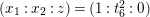
. Then, this family has a rational point
 $(1:t_{6}^{2}:0)$
(cf. Mestre [Reference MestreMe] and Kuwata–Wang [Reference Kuwata and WangKwW]). Using this point, we convert (2.2) to the Weierstrass form:
$(1:t_{6}^{2}:0)$
(cf. Mestre [Reference MestreMe] and Kuwata–Wang [Reference Kuwata and WangKwW]). Using this point, we convert (2.2) to the Weierstrass form:
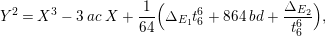 $$\begin{eqnarray}Y^{2}=X^{3}-3\,ac\,X+\frac{1}{64}\Bigl(\unicode[STIX]{x1D6E5}_{E_{1}}t_{6}^{6}+864\,bd+\frac{\unicode[STIX]{x1D6E5}_{E_{2}}}{t_{6}^{6}}\Bigr),\end{eqnarray}$$
where
 $\unicode[STIX]{x1D6E5}_{E_{1}}$
and
$\unicode[STIX]{x1D6E5}_{E_{1}}$
and
 $\unicode[STIX]{x1D6E5}_{E_{2}}$
are the discriminants of
$\unicode[STIX]{x1D6E5}_{E_{2}}$
are the discriminants of
 $E_{1}$
and
$E_{1}$
and
 $E_{2}$
, respectively:
$E_{2}$
, respectively:
 $$\begin{eqnarray}\unicode[STIX]{x1D6E5}_{E_{1}}=-16(4a^{3}+27b^{2}),\qquad \unicode[STIX]{x1D6E5}_{E_{2}}=-16(4c^{3}+27d^{2}).\end{eqnarray}$$
The change of coordinates between (2.2) and (2.3) are given by
 $$\begin{eqnarray}\displaystyle \left\{\begin{array}{@{}l@{}}\displaystyle X=\frac{-t_{6}^{2}(2at_{6}^{4}-c)x_{1}-3(bt_{6}^{6}-d)-(at_{6}^{4}-2c)x_{2}}{t_{6}^{2}(t_{6}^{2}x_{1}-x_{2})},\\ \displaystyle Y=\frac{6(at_{6}^{4}-c)(bt_{6}^{6}-d)+6(at_{6}^{4}-c)(at_{6}^{6}x_{1}-cx_{2})-9(bt_{6}^{6}-d)(t_{6}^{4}x_{1}^{2}-x_{2}^{2})}{2t_{6}^{3}(t_{6}^{2}x_{1}-x_{2})^{2}}.\end{array}\right. & & \displaystyle \nonumber\\ \displaystyle & & \displaystyle\end{eqnarray}$$
Note that if we choose other models of
 $E_{1}$
and
$E_{1}$
and
 $E_{2}$
, we still obtain an isomorphic equation. Indeed, if we replace the equations of
$E_{2}$
, we still obtain an isomorphic equation. Indeed, if we replace the equations of
 $E_{1}$
and
$E_{1}$
and
 $E_{2}$
by
$E_{2}$
by
 $$\begin{eqnarray}\displaystyle & & \displaystyle E_{1}:y^{2}=x^{3}+(k^{4}a)x+(k^{6}b),\nonumber\\ \displaystyle & & \displaystyle E_{2}:y^{2}=x^{3}+(l^{4}c)x+(l^{6}d),\nonumber\end{eqnarray}$$
then replacing
 $(X,Y,t_{6})$
by
$(X,Y,t_{6})$
by
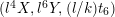 $(l^{4}X,l^{6}Y,(l/k)t_{6})$
, we recover equation (2.3).
$(l^{4}X,l^{6}Y,(l/k)t_{6})$
, we recover equation (2.3).
It is easy to see that equation (2.3) is invariant under the two automorphisms of the
 $t_{6}$
-line:
$t_{6}$
-line:
 $$\begin{eqnarray}\begin{array}{@{}l@{}}\unicode[STIX]{x1D70E}:t_{6}\mapsto \unicode[STIX]{x1D701}_{6}t_{6},\quad \text{where}~\unicode[STIX]{x1D701}_{6}~\text{is a primitive sixth root of unity},\\ \unicode[STIX]{x1D70F}:t_{6}\mapsto \unicode[STIX]{x1D6FF}/t_{6},\quad \text{where}~\unicode[STIX]{x1D6FF}~\text{is a chosen sixth root of}~\unicode[STIX]{x1D6E5}_{2}/\unicode[STIX]{x1D6E5}_{1}.\end{array}\end{eqnarray}$$
Taking the quotient by the action of
 $\unicode[STIX]{x1D70E}$
, or equivalently, setting
$\unicode[STIX]{x1D70E}$
, or equivalently, setting
 $t_{1}=t_{6}^{6}$
, we obtain an elliptic curve over the field
$t_{1}=t_{6}^{6}$
, we obtain an elliptic curve over the field
 $k(t_{1})$
, which we denote by
$k(t_{1})$
, which we denote by
 $F_{E_{1},E_{2}}^{(1)}$
:
$F_{E_{1},E_{2}}^{(1)}$
:
 $$\begin{eqnarray}F_{E_{1},E_{2}}^{(1)}:Y^{2}=X^{3}-3\,ac\,X+\frac{1}{64}\Bigl(\unicode[STIX]{x1D6E5}_{E_{1}}t_{1}+864\,bd+\frac{\unicode[STIX]{x1D6E5}_{E_{2}}}{t_{1}}\Bigr).\end{eqnarray}$$
Definition 2.1. The Kodaira–Néron model of the elliptic curve
 $F_{E_{1},E_{2}}^{(1)}$
over
$F_{E_{1},E_{2}}^{(1)}$
over
 $k(t_{1})$
defined by (2.6) is called the Inose surface associated with
$k(t_{1})$
defined by (2.6) is called the Inose surface associated with
 $E_{1}$
and
$E_{1}$
and
 $E_{2}$
, and it is denoted by
$E_{2}$
, and it is denoted by
 $\mathit{Ino}(E_{1},E_{2})$
.
$\mathit{Ino}(E_{1},E_{2})$
.
Remark 2.2. In [Reference Shioda and InoseSI], what we call the Inose surface in this article was originally constructed as a double cover of
 $\mathit{Km}(E_{1}\times E_{2})$
. Shioda and Inose then showed that the following diagram of rational maps, called a Shioda–Inose structure, induces an isomorphism of integral Hodge structures on the transcendental lattices of
$\mathit{Km}(E_{1}\times E_{2})$
. Shioda and Inose then showed that the following diagram of rational maps, called a Shioda–Inose structure, induces an isomorphism of integral Hodge structures on the transcendental lattices of
 $E_{1}\times E_{2}$
and
$E_{1}\times E_{2}$
and
 $\mathit{Ino}(E_{1},E_{2})$
.
$\mathit{Ino}(E_{1},E_{2})$
.
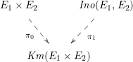
Since the Kodaira–Néron model of
 $F_{E_{1}\times E_{2}}^{(2)}$
is isomorphic to
$F_{E_{1}\times E_{2}}^{(2)}$
is isomorphic to
 $\mathit{Km}(E_{1}\times E_{2})$
over
$\mathit{Km}(E_{1}\times E_{2})$
over
 $\overline{k}$
(with
$\overline{k}$
(with
 $t_{2}$
being the elliptic parameter of the Inose fibration [Reference InoseI2]), we have another quotient map from
$t_{2}$
being the elliptic parameter of the Inose fibration [Reference InoseI2]), we have another quotient map from
 $\mathit{Km}(E_{1}\times E_{2})$
to
$\mathit{Km}(E_{1}\times E_{2})$
to
 $\mathit{Ino}(E_{1},E_{2})$
. Thus, we have a “Kummer sandwich” diagram:
$\mathit{Ino}(E_{1},E_{2})$
. Thus, we have a “Kummer sandwich” diagram:

(cf. Shioda [Reference ShiodaSh4]). However, with our definition of
 $\mathit{Ino}(E_{1},E_{2})$
, the quotient map
$\mathit{Ino}(E_{1},E_{2})$
, the quotient map
 $\unicode[STIX]{x1D70B}_{1}$
may not be defined over the base field
$\unicode[STIX]{x1D70B}_{1}$
may not be defined over the base field
 $k$
itself, but rather only over
$k$
itself, but rather only over
 $k(E_{1}[2],E_{2}[2])$
(or an extension of
$k(E_{1}[2],E_{2}[2])$
(or an extension of
 $k$
including some of the
$k$
including some of the
 $2$
-torsion of
$2$
-torsion of
 $E_{1}$
and
$E_{1}$
and
 $E_{2}$
).
$E_{2}$
).
Definition 2.3. For
 $n=1,\ldots ,6$
, let
$n=1,\ldots ,6$
, let
 $t_{n}$
be a parameter satisfying
$t_{n}$
be a parameter satisfying
 $t_{n}^{n}=t_{1}$
. Define the elliptic curve
$t_{n}^{n}=t_{1}$
. Define the elliptic curve
 $F_{E_{1},E_{2}}^{(n)}$
over
$F_{E_{1},E_{2}}^{(n)}$
over
 $k(t_{n})$
by
$k(t_{n})$
by
 $$\begin{eqnarray}F_{E_{1},E_{2}}^{(n)}:Y^{2}=X^{3}-3\,ac\,X+\frac{1}{64}\Bigl(\unicode[STIX]{x1D6E5}_{E_{1}}t_{n}^{n}+864\,bd+\frac{\unicode[STIX]{x1D6E5}_{E_{2}}}{t_{n}^{n}}\Bigr).\end{eqnarray}$$
When
 $E_{1}$
and
$E_{1}$
and
 $E_{2}$
are understood, we write
$E_{2}$
are understood, we write
 $F^{(n)}$
for short.
$F^{(n)}$
for short.
Remark 2.4. The Kodaira–Néron model of
 $F_{E_{1},E_{2}}^{(n)}$
is a K3 surface for
$F_{E_{1},E_{2}}^{(n)}$
is a K3 surface for
 $n=1,\ldots ,6$
, but not for
$n=1,\ldots ,6$
, but not for
 $n\geqslant 7$
.
$n\geqslant 7$
.
By Inose’s theorem [Reference InoseI1, Cor. 1.2], the Picard number of the K3 surface
 $F^{(n)}$
does not depend on
$F^{(n)}$
does not depend on
 $n$
, and equals the Picard number of the Kummer surface
$n$
, and equals the Picard number of the Kummer surface
 $\mathit{Km}(E_{1}\times E_{2})$
. It is therefore at least
$\mathit{Km}(E_{1}\times E_{2})$
. It is therefore at least
 $18$
. These surfaces are clearly of geometric and arithmetic interest, being closely related to abelian surfaces which are the product of two elliptic curves. We now summarize what is known about the geometric Picard and Mordell–Weil groups of these elliptic K3 surfaces.
$18$
. These surfaces are clearly of geometric and arithmetic interest, being closely related to abelian surfaces which are the product of two elliptic curves. We now summarize what is known about the geometric Picard and Mordell–Weil groups of these elliptic K3 surfaces.
Define
 $R(t)$
and
$R(t)$
and
 $S(t)$
by letting the Inose surface as in equation (2.6) be
$S(t)$
by letting the Inose surface as in equation (2.6) be
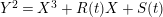 $Y^{2}=X^{3}+R(t)X+S(t)$
, and let
$Y^{2}=X^{3}+R(t)X+S(t)$
, and let
 $h=\operatorname{rank}\operatorname{Hom}(E_{1},E_{2})$
, so that
$h=\operatorname{rank}\operatorname{Hom}(E_{1},E_{2})$
, so that
 $0\leqslant h\leqslant 4$
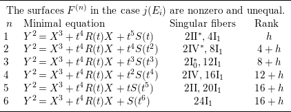
. The table below list the minimal Weierstrass equations, the configuration of singular fibers, and the Mordell–Weil rank in the “generic” case
$0\leqslant h\leqslant 4$
. The table below list the minimal Weierstrass equations, the configuration of singular fibers, and the Mordell–Weil rank in the “generic” case
 $j(E_{1})\neq j(E_{2})$
and
$j(E_{1})\neq j(E_{2})$
and
 $j(E_{i})\neq 0$
. In the other cases, which will not be relevant to this paper, we refer the reader to [Reference KuwataKw2, Th. 4.1] for the analogous data.
$j(E_{i})\neq 0$
. In the other cases, which will not be relevant to this paper, we refer the reader to [Reference KuwataKw2, Th. 4.1] for the analogous data.
The Néron–Severi and transcendental lattices were further analyzed by Shioda [Reference ShiodaSh3, Reference ShiodaSh5, Reference ShiodaSh7], culminating in the following theorems, which are stated in the geometric situation
 $k=\mathbb{C}$
. In this case we may scale
$k=\mathbb{C}$
. In this case we may scale
 $x,y,t$
to work with a simpler equation of
$x,y,t$
to work with a simpler equation of
 $F^{(n)}$
, as in [Reference InoseI1, Reference ShiodaSh3]:
$F^{(n)}$
, as in [Reference InoseI1, Reference ShiodaSh3]:
 $$\begin{eqnarray}Y^{2}=X^{3}-3\sqrt[3]{J_{1}J_{2}}\,X+t^{n}+\frac{1}{t^{n}}-2\sqrt{(1-J_{1})(1-J_{2})},\end{eqnarray}$$
where
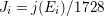 $J_{i}=j(E_{i})/1728$
.
$J_{i}=j(E_{i})/1728$
.
Theorem 2.5. (Shioda [Reference ShiodaSh5])
There is an isomorphism of lattices
 $T(F^{(n)})\cong T(F^{(1)})\langle n\rangle$
. In particular,
$T(F^{(n)})\cong T(F^{(1)})\langle n\rangle$
. In particular,
 $\det T(F^{(n)})=\det T(F^{(1)})\cdot n^{\unicode[STIX]{x1D706}}$
, where
$\det T(F^{(n)})=\det T(F^{(1)})\cdot n^{\unicode[STIX]{x1D706}}$
, where
 $\unicode[STIX]{x1D706}=4-h$
. The Mordell–Weil group
$\unicode[STIX]{x1D706}=4-h$
. The Mordell–Weil group
 $\operatorname{MW}(F^{(n)})$
is torsion-free, except when
$\operatorname{MW}(F^{(n)})$
is torsion-free, except when
 $j(E_{1})=j(E_{2})=0$
and
$j(E_{1})=j(E_{2})=0$
and
 $n=2,4,6$
, or
$n=2,4,6$
, or
 $j(E_{1})=j(E_{2})=1728$
and
$j(E_{1})=j(E_{2})=1728$
and
 $n=3,6$
.
$n=3,6$
.
Remark 2.6. The notation
 $\langle n\rangle$
means that the pairing of the lattice is multiplied by
$\langle n\rangle$
means that the pairing of the lattice is multiplied by
 $n$
.
$n$
.
Theorem 2.7. (Shioda [Reference ShiodaSh7])
There is a natural isomorphism of lattices
 $$\begin{eqnarray}\operatorname{Hom}(E_{1},E_{2})\cong F^{(1)}(k(t)).\end{eqnarray}$$
In particular, we can compute the Mordell–Weil rank as follows:
Proposition 2.8. [Reference ShiodaSh3]
For elliptic curves
 $E_{1}$
and
$E_{1}$
and
 $E_{2}$
, and
$E_{2}$
, and
 $1\leqslant n\leqslant 6$
, we have
$1\leqslant n\leqslant 6$
, we have
 $$\begin{eqnarray}\displaystyle \operatorname{rank}F_{E_{1},E_{2}}^{(n)}(\bar{k}(t_{n})) & = & \displaystyle h+\min (4(n-1),16)\nonumber\\ \displaystyle & & \displaystyle -\,\left\{\begin{array}{@{}ll@{}}0\quad & \text{if}~j(E_{1})\neq j(E_{2}),\\ n\quad & \text{if}~j(E_{1})=j(E_{2})\neq 0,1728,\\ 2n\quad & \text{if}~j(E_{1})=j(E_{2})=0~\text{or}~1728,\end{array}\right.\nonumber\end{eqnarray}$$
where
 $h=\operatorname{rank}\operatorname{Hom}(E_{1},E_{2})$
.
$h=\operatorname{rank}\operatorname{Hom}(E_{1},E_{2})$
.
In particular, the largest possible Mordell–Weil rank is
 $18$
, and we have the following.
$18$
, and we have the following.
Proposition 2.9. Let
 $E_{1}$
and
$E_{1}$
and
 $E_{2}$
be two elliptic curves over
$E_{2}$
be two elliptic curves over
 $k$
satisfying the following two conditions.
$k$
satisfying the following two conditions.
-
(i)
 $E_{1}$
and
$E_{2}$
are isogenous but not isomorphic over
$\overline{k}$
.
$E_{1}$
and
$E_{2}$
are isogenous but not isomorphic over
$\overline{k}$
. -
(ii)
$E_{1}$
and
$E_{2}$
have complex multiplication.


Then the Mordell–Weil groups
 $F^{(5)}(\overline{k}(t_{5}))$
and
$F^{(5)}(\overline{k}(t_{5}))$
and
 $F^{(6)}(\overline{k}(t_{6}))$
have rank
$F^{(6)}(\overline{k}(t_{6}))$
have rank
 $18$
.
$18$
.
Shioda further analyzed the surface
 $F^{(5)}$
for the CM elliptic curves
$F^{(5)}$
for the CM elliptic curves
 $y^{2}=x^{3}-1$
and
$y^{2}=x^{3}-1$
and
 $y^{2}=x^{3}-15x+22$
, which are
$y^{2}=x^{3}-15x+22$
, which are
 $2$
-isogenous to each other, and determined its Mordell–Weil group [Reference ShiodaSh6]. For the same pair of elliptic curves,
$2$
-isogenous to each other, and determined its Mordell–Weil group [Reference ShiodaSh6]. For the same pair of elliptic curves,
 $F^{(6)}$
was studied in [Reference Chahal, Meijer and TopCMT] and generators for its Mordell–Weil group were computed.
$F^{(6)}$
was studied in [Reference Chahal, Meijer and TopCMT] and generators for its Mordell–Weil group were computed.
In this article, we will generalize these results further, to obtain explicit descriptions of the Mordell–Weil lattices of the surfaces
 $F^{(n)}$
. Our main results are the following.
$F^{(n)}$
. Our main results are the following.
Theorem 2.10. Suppose the two elliptic curves
 $E_{1}$
and
$E_{1}$
and
 $E_{2}$
are not isogenous (over
$E_{2}$
are not isogenous (over
 $\overline{k}$
).
$\overline{k}$
).
-
(i) The field of definition of the Mordell–Weil group of
$F^{(n)}$
(i.e., the smallest field over which all the sections are defined) is contained in
$k(E_{1}[n],E_{2}[n])$
, the compositum of the
$n$
-torsion fields of
$E_{1}$
and
$E_{2}$
. -
(ii) An explicit basis for
$\operatorname{MW}(F^{n})$
is described by the corresponding results: Proposition 3.3, Theorems 4.8, 5.1, 5.3, 6.4, 7.1 and 7.11.


Theorem 2.11. In the general case when
 $E_{1}$
and
$E_{1}$
and
 $E_{2}$
are allowed to be isogenous, there is a finite index sublattice
$E_{2}$
are allowed to be isogenous, there is a finite index sublattice
 $\operatorname{MW}(F^{n})$
for which all the sections can be defined over the compositum of
$\operatorname{MW}(F^{n})$
for which all the sections can be defined over the compositum of
 $k(E_{1}[n],E_{2}[n])$
and the field of definition of
$k(E_{1}[n],E_{2}[n])$
and the field of definition of
 $\operatorname{Hom}(E_{1},E_{2})$
.
$\operatorname{Hom}(E_{1},E_{2})$
.
Remark 2.12. It is possible that the field of definition of
 $\operatorname{MW}(F^{n})$
in the general case coincides with the above compositum. However, we have not generated sufficient numerical evidence to formally state this as a conjecture.
$\operatorname{MW}(F^{n})$
in the general case coincides with the above compositum. However, we have not generated sufficient numerical evidence to formally state this as a conjecture.
2.2 Galois correspondence of sublattices
The Mordell–Weil lattice of the surface
 $F^{(6)}$
has a particularly rich structure, with sublattices induced from the Mordell–Weil lattices of several quotients which are elliptic rational or K3 surfaces. As we saw in (2.5), a dihedral group
$F^{(6)}$
has a particularly rich structure, with sublattices induced from the Mordell–Weil lattices of several quotients which are elliptic rational or K3 surfaces. As we saw in (2.5), a dihedral group
 $D_{6}$
generated by
$D_{6}$
generated by
 $\unicode[STIX]{x1D70E}$
and
$\unicode[STIX]{x1D70E}$
and
 $\unicode[STIX]{x1D70F}$
acts on
$\unicode[STIX]{x1D70F}$
acts on
 $F^{(6)}$
. We define
$F^{(6)}$
. We define
 $$\begin{eqnarray}s_{n,i}=t_{n}+\frac{(\unicode[STIX]{x1D701}_{6}^{-i}\unicode[STIX]{x1D6FF})^{6/n}}{t_{n}},\quad n=1,2,3,6,\;i=0,1,\ldots ,n-1.\end{eqnarray}$$
Recall that
 $t_{n}^{n}=t_{1}=t_{6}^{6}$
. Then
$t_{n}^{n}=t_{1}=t_{6}^{6}$
. Then
 $s_{n,i}$
is invariant under
$s_{n,i}$
is invariant under
 $\unicode[STIX]{x1D70E}^{n}$
and
$\unicode[STIX]{x1D70E}^{n}$
and
 $\unicode[STIX]{x1D70F}\unicode[STIX]{x1D70E}^{i}$
. Write
$\unicode[STIX]{x1D70F}\unicode[STIX]{x1D70E}^{i}$
. Write
 $S=s_{1,0}=t_{1}+(\unicode[STIX]{x1D6E5}_{E_{2}}/\unicode[STIX]{x1D6E5}_{E_{1}})t_{1}^{-1}$
for simplicity. Then, the extension
$S=s_{1,0}=t_{1}+(\unicode[STIX]{x1D6E5}_{E_{2}}/\unicode[STIX]{x1D6E5}_{E_{1}})t_{1}^{-1}$
for simplicity. Then, the extension
 $k(t_{6})/k(S)$
is a Galois extension, and its Galois group is
$k(t_{6})/k(S)$
is a Galois extension, and its Galois group is
 $D_{6}=\langle \unicode[STIX]{x1D70E},\unicode[STIX]{x1D70F}\rangle$
. Our basic idea is to consider the elliptic surface
$D_{6}=\langle \unicode[STIX]{x1D70E},\unicode[STIX]{x1D70F}\rangle$
. Our basic idea is to consider the elliptic surface
 $$\begin{eqnarray}F_{S}:Y^{2}=X^{3}-{\textstyle \frac{1}{3}}A\,X+{\textstyle \frac{1}{64}}(\unicode[STIX]{x1D6E5}_{E_{1}}S+C),\end{eqnarray}$$
where
 $A$
and
$A$
and
 $C$
are as in (2.8), and view
$C$
are as in (2.8), and view
 $F^{(6)}(\bar{k}(t_{6}))$
as the Mordell–Weil group of
$F^{(6)}(\bar{k}(t_{6}))$
as the Mordell–Weil group of
 $F_{S}$
over the extension
$F_{S}$
over the extension
 $\bar{k}(t_{6})/\bar{k}(S)$
. In other words, we regard
$\bar{k}(t_{6})/\bar{k}(S)$
. In other words, we regard
 $F^{(6)}(\bar{k}(t_{6}))=F_{S}(\bar{k}(t_{6}))$
.
$F^{(6)}(\bar{k}(t_{6}))=F_{S}(\bar{k}(t_{6}))$
.
Write
 $M(t_{n})=F_{S}(\bar{k}(t_{n}))$
and
$M(t_{n})=F_{S}(\bar{k}(t_{n}))$
and
 $M(s_{n,i})=F_{S}(\bar{k}(s_{n,i}))$
. Between
$M(s_{n,i})=F_{S}(\bar{k}(s_{n,i}))$
. Between
 $k(t_{6})$
and
$k(t_{6})$
and
 $k(S)$
there are fourteen intermediate fields. Corresponding to these we have a relation among the Mordell–Weil groups
$k(S)$
there are fourteen intermediate fields. Corresponding to these we have a relation among the Mordell–Weil groups
 $M(t_{n})$
and
$M(t_{n})$
and
 $M(s_{n,i})$
.
$M(s_{n,i})$
.

For later use, let us write a more general formula for
 $F^{(n)}$
. If
$F^{(n)}$
. If
 $E_{1}$
and
$E_{1}$
and
 $E_{2}$
are given by
$E_{2}$
are given by
 $$\begin{eqnarray}\displaystyle E_{1}:y^{2} & = & \displaystyle x^{3}+a_{2}x^{2}+a_{4}x+a_{6},\nonumber\\ \displaystyle E_{2}:y^{2} & = & \displaystyle x^{3}+a_{2}^{\prime }x^{2}+a_{4}^{\prime }x+a_{6}^{\prime },\nonumber\end{eqnarray}$$
then the equation of
 $F_{E_{1},E_{2}}^{(n)}$
is given by
$F_{E_{1},E_{2}}^{(n)}$
is given by
 $$\begin{eqnarray}F_{E_{1},E_{2}}^{(n)}:Y^{2}=X^{3}-\frac{1}{3}A\,X+\frac{1}{64}\left(B\,t_{n}^{n}+C+\frac{D}{t_{n}^{n}}\right),\end{eqnarray}$$
where
 $$\begin{eqnarray}\left\{\begin{array}{@{}l@{}}A=(a_{2}^{2}-3a_{4})({a_{2}^{\prime }}^{2}-3a_{4}^{\prime }),\\ B=16(a_{2}^{2}a_{4}^{2}-4a_{2}^{3}a_{6}+18a_{2}a_{4}a_{6}-4a_{4}^{3}-27a_{6}^{2})=\unicode[STIX]{x1D6E5}_{E_{1}},\\ C=\frac{32}{27}(2a_{2}^{3}-9a_{2}a_{4}+27a_{6})(2{a_{2}^{\prime }}^{3}-9a_{2}^{\prime }a_{4}^{\prime }+27a_{6}^{\prime }),\\ D=16({a_{2}^{\prime }}^{2}{a_{4}^{\prime }}^{2}-4{a_{2}^{\prime }}^{3}a_{6}^{\prime }+18a_{2}^{\prime }a_{4}^{\prime }a_{6}^{\prime }-4{a_{4}^{\prime }}^{3}-27{a_{6}^{\prime }}^{2})=\unicode[STIX]{x1D6E5}_{E_{2}}.\end{array}\right.\end{eqnarray}$$
3 The Mordell–Weil groups of
$F^{(1)}$
and
$F^{(2)}$


In this section we summarize the description of the Mordell–Weil lattices
 $F^{(1)}(\overline{k}(t_{1}))$
and
$F^{(1)}(\overline{k}(t_{1}))$
and
 $F^{(2)}(\overline{k}(t_{2}))$
for completeness.
$F^{(2)}(\overline{k}(t_{2}))$
for completeness.
3.1
$F^{(1)}$
for isogenous case

The Mordell–Weil lattice of
 $F^{(1)}(\overline{k}(t_{1}))$
for generic
$F^{(1)}(\overline{k}(t_{1}))$
for generic
 $E_{1}$
and
$E_{1}$
and
 $E_{2}$
is trivial, and we have nothing to do. If
$E_{2}$
is trivial, and we have nothing to do. If
 $E_{1}$
and
$E_{1}$
and
 $E_{2}$
are isogenous but not isomorphic over
$E_{2}$
are isogenous but not isomorphic over
 $\overline{k}$
, we have the following interpretation of the Mordell–Weil lattice by
$\overline{k}$
, we have the following interpretation of the Mordell–Weil lattice by
 $\operatorname{Hom}(E_{1},E_{2})$
.
$\operatorname{Hom}(E_{1},E_{2})$
.
Proposition 3.1. (Shioda [Reference ShiodaSh5])
Let
 $E_{1}$
and
$E_{1}$
and
 $E_{2}$
be two elliptic curves not isomorphic to each other over
$E_{2}$
be two elliptic curves not isomorphic to each other over
 $\overline{k}$
. Then, the Mordell–Weil lattice of
$\overline{k}$
. Then, the Mordell–Weil lattice of
 $F^{(1)}(\overline{k}(t_{1}))$
is isomorphic to the lattice
$F^{(1)}(\overline{k}(t_{1}))$
is isomorphic to the lattice
 $\operatorname{Hom}(E_{1},E_{2})\langle 2\rangle$
, where the pairing of
$\operatorname{Hom}(E_{1},E_{2})\langle 2\rangle$
, where the pairing of
 $\operatorname{Hom}(E_{1},E_{2})$
is given by
$\operatorname{Hom}(E_{1},E_{2})$
is given by
 $$\begin{eqnarray}(\unicode[STIX]{x1D711},\unicode[STIX]{x1D713})={\textstyle \frac{1}{2}}(\deg (\unicode[STIX]{x1D711}+\unicode[STIX]{x1D713})-\deg \unicode[STIX]{x1D711}-\deg \unicode[STIX]{x1D713})\quad \unicode[STIX]{x1D711},\unicode[STIX]{x1D713}\in \operatorname{Hom}(E_{1},E_{2}).\end{eqnarray}$$
For a given
 $\unicode[STIX]{x1D711}\in \operatorname{Hom}(E_{1},E_{2})$
, we would like to compute the section corresponding to
$\unicode[STIX]{x1D711}\in \operatorname{Hom}(E_{1},E_{2})$
, we would like to compute the section corresponding to
 $\unicode[STIX]{x1D711}$
explicitly. To do so, we consider the inclusion
$\unicode[STIX]{x1D711}$
explicitly. To do so, we consider the inclusion
 $$\begin{eqnarray}\operatorname{Hom}(E_{1},E_{2})\langle 2\rangle \simeq F_{E_{1},E_{2}}^{(1)}(\bar{k}(t_{1})){\hookrightarrow}\operatorname{Hom}(E_{1},E_{2})\langle 12\rangle \subset F_{E_{1},E_{2}}^{(6)}(\bar{k}(t_{6}))\end{eqnarray}$$
induced by
 $t_{1}\mapsto t_{6}^{6}$
, and we look for a section in
$t_{1}\mapsto t_{6}^{6}$
, and we look for a section in
 $F_{E_{1},E_{2}}^{(6)}(\bar{k}(t_{6}))$
.
$F_{E_{1},E_{2}}^{(6)}(\bar{k}(t_{6}))$
.
Suppose
 $E_{1}$
and
$E_{1}$
and
 $E_{2}$
are given in the form of (2.1). By replacing
$E_{2}$
are given in the form of (2.1). By replacing
 $t_{2}$
by
$t_{2}$
by
 $t_{6}^{3}$
in the equation of Kummer surface (2.2), we regard it as a cubic curve over
$t_{6}^{3}$
in the equation of Kummer surface (2.2), we regard it as a cubic curve over
 $k(t_{6})$
. More precisely, we consider the cubic curve in the projective plane over
$k(t_{6})$
. More precisely, we consider the cubic curve in the projective plane over
 $k(t_{6})$
with coordinates
$k(t_{6})$
with coordinates
 $(x_{1}:x_{2}:z)$
defined by
$(x_{1}:x_{2}:z)$
defined by
 $$\begin{eqnarray}C_{t_{6}}:x_{2}^{3}+cx_{2}z^{2}+dz^{3}=t_{6}^{6}(x_{1}^{3}+ax_{1}z^{2}+bz^{3}).\end{eqnarray}$$
Suppose
 $\unicode[STIX]{x1D711}$
is an isogeny of degree
$\unicode[STIX]{x1D711}$
is an isogeny of degree
 $d$
. Then,
$d$
. Then,
 $\unicode[STIX]{x1D711}$
can be written in the form
$\unicode[STIX]{x1D711}$
can be written in the form
 $$\begin{eqnarray}\unicode[STIX]{x1D711}:(x_{1},y_{1})\mapsto (x_{2},y_{2})=(\unicode[STIX]{x1D711}_{x}(x_{1}),\unicode[STIX]{x1D711}_{y}(x_{1})y_{1}).\end{eqnarray}$$
Consider the curve of degree
 $d$
given by
$d$
given by
 $x_{2}=\unicode[STIX]{x1D711}_{x}(x_{1})$
. The intersection of these two curves
$x_{2}=\unicode[STIX]{x1D711}_{x}(x_{1})$
. The intersection of these two curves
 $$\begin{eqnarray}\left\{\begin{array}{@{}l@{}}x_{2}^{3}+cx_{2}+d=t_{6}^{6}(x_{1}^{3}+ax_{1}+b),\\ x_{2}=\unicode[STIX]{x1D711}_{x}(x_{1}),\end{array}\right.\end{eqnarray}$$
gives a divisor of degree
 $3d$
in
$3d$
in
 $C_{t_{6}}$
. Since we have
$C_{t_{6}}$
. Since we have
 $\unicode[STIX]{x1D711}_{x}(x_{1})^{3}+c\unicode[STIX]{x1D711}_{x}(x_{1})+d=\unicode[STIX]{x1D711}_{y}(x_{1})^{2}y_{1}^{2}=\unicode[STIX]{x1D711}_{y}(x_{1})^{2}(x_{1}^{3}+ax_{1}+b),$
the first equation reduces to
$\unicode[STIX]{x1D711}_{x}(x_{1})^{3}+c\unicode[STIX]{x1D711}_{x}(x_{1})+d=\unicode[STIX]{x1D711}_{y}(x_{1})^{2}y_{1}^{2}=\unicode[STIX]{x1D711}_{y}(x_{1})^{2}(x_{1}^{3}+ax_{1}+b),$
the first equation reduces to
 $$\begin{eqnarray}(\unicode[STIX]{x1D711}_{y}(x_{1})-t_{6}^{3})(\unicode[STIX]{x1D711}_{y}(x_{1})+t_{6}^{3})(x_{1}^{3}+ax_{1}+b)=0.\end{eqnarray}$$
Proposition 3.2. Let
 $\unicode[STIX]{x1D711}:E_{1}\rightarrow E_{2}$
be an isogeny of degree
$\unicode[STIX]{x1D711}:E_{1}\rightarrow E_{2}$
be an isogeny of degree
 $d$
defined over
$d$
defined over
 $k$
. Let
$k$
. Let
 $D_{\unicode[STIX]{x1D711}}^{+}$
(resp.
$D_{\unicode[STIX]{x1D711}}^{+}$
(resp.
 $D_{\unicode[STIX]{x1D711}}^{-}$
) be the divisor on the cubic curve (3.1) defined by the equation
$D_{\unicode[STIX]{x1D711}}^{-}$
) be the divisor on the cubic curve (3.1) defined by the equation
 $\unicode[STIX]{x1D711}_{y}(x_{1})=t_{6}^{3}$
(resp.
$\unicode[STIX]{x1D711}_{y}(x_{1})=t_{6}^{3}$
(resp.
 $\unicode[STIX]{x1D711}_{y}(x_{1})=-t_{6}^{3}$
).
$\unicode[STIX]{x1D711}_{y}(x_{1})=-t_{6}^{3}$
).
-
(i) The divisor
$D_{\unicode[STIX]{x1D711}}^{+}$
(resp.
$D_{\unicode[STIX]{x1D711}}^{-}$
) determines a
$k(t_{6})$
-rational point
$P_{\unicode[STIX]{x1D711}}^{+}$
(resp.
$P_{\unicode[STIX]{x1D711}}^{-}$
) in
$F^{(6)}(k(t_{6}))$
. -
(ii)
$P_{\unicode[STIX]{x1D711}}^{+}-P_{\unicode[STIX]{x1D711}}^{-}$
is in the image of
$F^{(1)}(k(t_{1}))\rightarrow F^{(6)}(k(t_{6}))$
. The height of its pre-image in
$F^{(1)}(k(t_{1}))$
is
$2d$
.


Proof. (i) If
 $d$
is odd, the denominator of
$d$
is odd, the denominator of
 $\unicode[STIX]{x1D711}_{y}(x_{1})$
and
$\unicode[STIX]{x1D711}_{y}(x_{1})$
and
 $x_{1}^{3}+ax_{1}+b$
are relatively prime. So, the degree of
$x_{1}^{3}+ax_{1}+b$
are relatively prime. So, the degree of
 $\unicode[STIX]{x1D711}_{y}(x_{1})=\pm t_{6}^{3}$
in
$\unicode[STIX]{x1D711}_{y}(x_{1})=\pm t_{6}^{3}$
in
 $x_{1}$
equals
$x_{1}$
equals
 $(3d-3)/2$
. If
$(3d-3)/2$
. If
 $d$
is even, a cancelation occurs between the denominator of
$d$
is even, a cancelation occurs between the denominator of
 $\unicode[STIX]{x1D711}_{y}(x_{1})$
and
$\unicode[STIX]{x1D711}_{y}(x_{1})$
and
 $x_{1}^{3}+ax_{1}+b$
at the
$x_{1}^{3}+ax_{1}+b$
at the
 $x_{1}$
coordinate of one of the
$x_{1}$
coordinate of one of the
 $2$
-torsion points of
$2$
-torsion points of
 $E_{1}$
. So, the degree of
$E_{1}$
. So, the degree of
 $\unicode[STIX]{x1D711}_{y}(x_{1})=\pm t_{6}^{3}$
equals
$\unicode[STIX]{x1D711}_{y}(x_{1})=\pm t_{6}^{3}$
equals
 $(3d-2)/2$
. In any case, let
$(3d-2)/2$
. In any case, let
 $r$
be the degree of
$r$
be the degree of
 $\unicode[STIX]{x1D711}_{y}(x_{1})=\pm t_{6}^{3}$
.
$\unicode[STIX]{x1D711}_{y}(x_{1})=\pm t_{6}^{3}$
.
Write
 $D_{\unicode[STIX]{x1D711}}^{+}=Q_{1}^{+}+\cdots +Q_{r}^{+}$
. (Note that the
$D_{\unicode[STIX]{x1D711}}^{+}=Q_{1}^{+}+\cdots +Q_{r}^{+}$
. (Note that the
 $Q_{i}^{+}$
are defined over an algebraic closure of
$Q_{i}^{+}$
are defined over an algebraic closure of
 $\bar{k}(t_{6})$
.) Recall that we chose
$\bar{k}(t_{6})$
.) Recall that we chose
 $(x_{1}:x_{2}:z)=(1:t_{6}^{2}:0)$
as the origin
$(x_{1}:x_{2}:z)=(1:t_{6}^{2}:0)$
as the origin
 $O$
of the group law on
$O$
of the group law on
 $C_{t_{6}}$
. We identify
$C_{t_{6}}$
. We identify
 $F_{E_{1},E_{2}}^{(6)}(\overline{k(t_{6})})$
with the divisor class group
$F_{E_{1},E_{2}}^{(6)}(\overline{k(t_{6})})$
with the divisor class group
 $\operatorname{Pic}_{\overline{k(t_{6})}}^{0}(C_{t_{6}})$
by the usual map which associates a section with its generic fiber minus
$\operatorname{Pic}_{\overline{k(t_{6})}}^{0}(C_{t_{6}})$
by the usual map which associates a section with its generic fiber minus
 $O$
. Let
$O$
. Let
 $Q_{\unicode[STIX]{x1D711}}^{+}$
be the point in
$Q_{\unicode[STIX]{x1D711}}^{+}$
be the point in
 $C_{t_{6}}$
such that
$C_{t_{6}}$
such that
 $D_{\unicode[STIX]{x1D711}}^{+}-rO\sim Q_{\unicode[STIX]{x1D711}}^{+}-O$
. Since
$D_{\unicode[STIX]{x1D711}}^{+}-rO\sim Q_{\unicode[STIX]{x1D711}}^{+}-O$
. Since
 $D_{\unicode[STIX]{x1D711}}^{+}$
and
$D_{\unicode[STIX]{x1D711}}^{+}$
and
 $O$
are defined over
$O$
are defined over
 $k(t_{6})$
, so is
$k(t_{6})$
, so is
 $Q_{\unicode[STIX]{x1D711}}^{+}$
. Thus, we have a point
$Q_{\unicode[STIX]{x1D711}}^{+}$
. Thus, we have a point
 $P_{\unicode[STIX]{x1D711}}^{+}=[Q_{\unicode[STIX]{x1D711}}^{+}-O]\in \operatorname{Pic}_{k(t_{6})}^{0}(C_{t_{6}})=F_{E_{1},E_{2}}^{(6)}(k(t_{6}))$
. Similarly, we obtain
$P_{\unicode[STIX]{x1D711}}^{+}=[Q_{\unicode[STIX]{x1D711}}^{+}-O]\in \operatorname{Pic}_{k(t_{6})}^{0}(C_{t_{6}})=F_{E_{1},E_{2}}^{(6)}(k(t_{6}))$
. Similarly, we obtain
 $P_{\unicode[STIX]{x1D711}}^{-}\in F_{E_{1},E_{2}}^{(6)}(k(t_{6}))$
from
$P_{\unicode[STIX]{x1D711}}^{-}\in F_{E_{1},E_{2}}^{(6)}(k(t_{6}))$
from
 $D_{\unicode[STIX]{x1D711}}^{-}$
.
$D_{\unicode[STIX]{x1D711}}^{-}$
.
(ii) By definition, the surface
 $F_{E_{1},E_{2}}^{(1)}$
is obtained as the quotient of
$F_{E_{1},E_{2}}^{(1)}$
is obtained as the quotient of
 $F_{E_{1},E_{2}}^{(6)}$
by the action
$F_{E_{1},E_{2}}^{(6)}$
by the action
 $(X,Y,t_{6})\mapsto (X,Y,\unicode[STIX]{x1D701}_{6}t_{6})$
on (2.3), where
$(X,Y,t_{6})\mapsto (X,Y,\unicode[STIX]{x1D701}_{6}t_{6})$
on (2.3), where
 $\unicode[STIX]{x1D701}_{6}$
is a primitive sixth root of unity. However, the action
$\unicode[STIX]{x1D701}_{6}$
is a primitive sixth root of unity. However, the action
 $\unicode[STIX]{x1D70E}:((x_{1}:x_{2}:z),t_{6})\mapsto ((x_{1}:x_{2}:z),\unicode[STIX]{x1D701}_{6}t_{6})$
on
$\unicode[STIX]{x1D70E}:((x_{1}:x_{2}:z),t_{6})\mapsto ((x_{1}:x_{2}:z),\unicode[STIX]{x1D701}_{6}t_{6})$
on
 $C_{t_{6}}$
does not correspond to
$C_{t_{6}}$
does not correspond to
 $(X,Y,t_{6})\mapsto (X,Y,\unicode[STIX]{x1D701}_{6}t_{6})$
since the quotient of the former gives a rational surface. As a matter of fact, calculations show that the action
$(X,Y,t_{6})\mapsto (X,Y,\unicode[STIX]{x1D701}_{6}t_{6})$
since the quotient of the former gives a rational surface. As a matter of fact, calculations show that the action
 $\unicode[STIX]{x1D70E}$
corresponds to the action
$\unicode[STIX]{x1D70E}$
corresponds to the action
 $(X,Y,t_{6})\mapsto (X,-Y,\unicode[STIX]{x1D701}_{6}t_{6})$
.
$(X,Y,t_{6})\mapsto (X,-Y,\unicode[STIX]{x1D701}_{6}t_{6})$
.
By construction, the involution
 $\unicode[STIX]{x1D70E}^{3}$
interchanges between the points
$\unicode[STIX]{x1D70E}^{3}$
interchanges between the points
 $Q_{\unicode[STIX]{x1D711}}^{+}$
and
$Q_{\unicode[STIX]{x1D711}}^{+}$
and
 $Q_{\unicode[STIX]{x1D711}}^{-}$
in
$Q_{\unicode[STIX]{x1D711}}^{-}$
in
 $C_{t_{6}}$
. Thus, the corresponding involution
$C_{t_{6}}$
. Thus, the corresponding involution
 $(X,Y,t_{6})\mapsto (X,-Y,-t_{6})$
on
$(X,Y,t_{6})\mapsto (X,-Y,-t_{6})$
on
 $F_{E_{1},E_{2}}^{(6)}$
sends
$F_{E_{1},E_{2}}^{(6)}$
sends
 $P_{\unicode[STIX]{x1D711}}^{+}$
to
$P_{\unicode[STIX]{x1D711}}^{+}$
to
 $P_{\unicode[STIX]{x1D711}}^{-}$
. This implies that
$P_{\unicode[STIX]{x1D711}}^{-}$
. This implies that
 $P_{\unicode[STIX]{x1D711}}^{+}-P_{\unicode[STIX]{x1D711}}^{-}$
is invariant under the involution
$P_{\unicode[STIX]{x1D711}}^{+}-P_{\unicode[STIX]{x1D711}}^{-}$
is invariant under the involution
 $(X,Y,t_{6})\mapsto (X,Y,-t_{6})$
. Moreover, since
$(X,Y,t_{6})\mapsto (X,Y,-t_{6})$
. Moreover, since
 $Q_{\unicode[STIX]{x1D711}}^{\pm }$
are both invariant under the automorphism
$Q_{\unicode[STIX]{x1D711}}^{\pm }$
are both invariant under the automorphism
 $\unicode[STIX]{x1D70E}^{2}$
by construction,
$\unicode[STIX]{x1D70E}^{2}$
by construction,
 $P_{\unicode[STIX]{x1D711}}^{\pm }$
are also invariant under the corresponding action. We thus conclude that
$P_{\unicode[STIX]{x1D711}}^{\pm }$
are also invariant under the corresponding action. We thus conclude that
 $P_{\unicode[STIX]{x1D711}}^{+}-P_{\unicode[STIX]{x1D711}}^{-}$
is invariant under
$P_{\unicode[STIX]{x1D711}}^{+}-P_{\unicode[STIX]{x1D711}}^{-}$
is invariant under
 $(X,Y,t_{6})\mapsto (X,Y,\unicode[STIX]{x1D701}_{6}t_{6})$
, and it belongs to the image of
$(X,Y,t_{6})\mapsto (X,Y,\unicode[STIX]{x1D701}_{6}t_{6})$
, and it belongs to the image of
 $F_{E_{1},E_{2}}^{(1)}(k(t_{6}))$
under the map
$F_{E_{1},E_{2}}^{(1)}(k(t_{6}))$
under the map
 $t_{1}\mapsto t_{6}^{6}$
.
$t_{1}\mapsto t_{6}^{6}$
.
It remains to calculate the height of this point, but the calculation is essentially the same as in [Reference ShiodaSh5, Proposition 3.1]. ◻
To compute
 $P_{\unicode[STIX]{x1D711}}^{\pm }$
explicitly, we need to find a curve in the plane passing through the points in the divisor
$P_{\unicode[STIX]{x1D711}}^{\pm }$
explicitly, we need to find a curve in the plane passing through the points in the divisor
 $D_{\unicode[STIX]{x1D711}}^{\pm }$
, and this is in principle just an exercise in linear algebra. We shall illustrate it using a concrete example (see Example 9.2).
$D_{\unicode[STIX]{x1D711}}^{\pm }$
, and this is in principle just an exercise in linear algebra. We shall illustrate it using a concrete example (see Example 9.2).
3.2
$F^{(2)}$
for generic case

Suppose two elliptic curves are given by
 $$\begin{eqnarray}\begin{array}{@{}l@{}}E_{\unicode[STIX]{x1D706}}:y^{2}=x(x-1)(x-\unicode[STIX]{x1D706}),\\ E_{\unicode[STIX]{x1D707}}:y^{2}=x(x-1)(x-\unicode[STIX]{x1D707})\end{array}\end{eqnarray}$$
for
 $\unicode[STIX]{x1D706},\unicode[STIX]{x1D707}\in \overline{k}$
. Then,
$\unicode[STIX]{x1D706},\unicode[STIX]{x1D707}\in \overline{k}$
. Then,
 $F_{E_{\unicode[STIX]{x1D706}},E_{\unicode[STIX]{x1D707}}}^{(2)}$
is given by the Weierstrass equation
$F_{E_{\unicode[STIX]{x1D706}},E_{\unicode[STIX]{x1D707}}}^{(2)}$
is given by the Weierstrass equation
 $$\begin{eqnarray}\displaystyle F_{E_{\unicode[STIX]{x1D706}},E_{\unicode[STIX]{x1D707}}}^{(2)}:Y^{2} & = & \displaystyle X^{3}-\frac{1}{3}(\unicode[STIX]{x1D707}^{2}-\unicode[STIX]{x1D707}+1)(\unicode[STIX]{x1D706}^{2}-\unicode[STIX]{x1D706}+1)X\nonumber\\ \displaystyle & & \displaystyle +\,\frac{1}{4}\unicode[STIX]{x1D706}^{2}(\unicode[STIX]{x1D706}-1)^{2}t^{2}+\frac{\unicode[STIX]{x1D707}^{2}(\unicode[STIX]{x1D707}-1)^{2}}{4t^{2}}\nonumber\\ \displaystyle & & \displaystyle +\,\frac{1}{54}(2\unicode[STIX]{x1D707}-1)(\unicode[STIX]{x1D707}-2)(\unicode[STIX]{x1D707}+1)(2\unicode[STIX]{x1D706}-1)(\unicode[STIX]{x1D706}-2)(\unicode[STIX]{x1D706}+1).\end{eqnarray}$$
Here, we wrote
 $t_{2}=t$
for simplicity. Note that in this case the equation of the Kummer surface
$t_{2}=t$
for simplicity. Note that in this case the equation of the Kummer surface
 $x_{2}(x_{2}-1)(x_{2}-\unicode[STIX]{x1D707})=t_{2}^{2}x_{1}(x_{1}-1)(x_{1}-\unicode[STIX]{x1D706})$
can be converted over
$x_{2}(x_{2}-1)(x_{2}-\unicode[STIX]{x1D707})=t_{2}^{2}x_{1}(x_{1}-1)(x_{1}-\unicode[STIX]{x1D706})$
can be converted over
 $k(\unicode[STIX]{x1D706},\unicode[STIX]{x1D707})$
to the Weierstrass form
$k(\unicode[STIX]{x1D706},\unicode[STIX]{x1D707})$
to the Weierstrass form
 $F^{(2)}$
using the point
$F^{(2)}$
using the point
 $(x_{1},x_{2})=(0,0)$
. Then we can obtain sections from
$(x_{1},x_{2})=(0,0)$
. Then we can obtain sections from
 $2$
-torsion points of
$2$
-torsion points of
 $E_{\unicode[STIX]{x1D706}}$
and
$E_{\unicode[STIX]{x1D706}}$
and
 $E_{\unicode[STIX]{x1D707}}$
. In the following proposition,
$E_{\unicode[STIX]{x1D707}}$
. In the following proposition,
 $P_{1},\ldots ,P_{4}$
are obtained from
$P_{1},\ldots ,P_{4}$
are obtained from
 $(x_{1},x_{2})=(1,1),(\unicode[STIX]{x1D706},\unicode[STIX]{x1D707}),(1,\unicode[STIX]{x1D707}),(\unicode[STIX]{x1D706},1)$
, respectively.
$(x_{1},x_{2})=(1,1),(\unicode[STIX]{x1D706},\unicode[STIX]{x1D707}),(1,\unicode[STIX]{x1D707}),(\unicode[STIX]{x1D706},1)$
, respectively.
Proposition 3.3. Suppose
 $E_{\unicode[STIX]{x1D706}}$
and
$E_{\unicode[STIX]{x1D706}}$
and
 $E_{\unicode[STIX]{x1D707}}$
are not isogenous over
$E_{\unicode[STIX]{x1D707}}$
are not isogenous over
 $\bar{k}$
. Then the following sections form a basis of the Mordell–Weil group
$\bar{k}$
. Then the following sections form a basis of the Mordell–Weil group
 $F_{E_{\unicode[STIX]{x1D706}},E_{\unicode[STIX]{x1D707}}}^{(2)}(\bar{k}(t))$
 $$\begin{eqnarray}\displaystyle P_{1} & = & \displaystyle \bigg(\frac{1}{3}(-2\unicode[STIX]{x1D706}\unicode[STIX]{x1D707}+\unicode[STIX]{x1D706}+\unicode[STIX]{x1D707}+1),\frac{1}{2}\unicode[STIX]{x1D706}(\unicode[STIX]{x1D706}-1)t+\frac{\unicode[STIX]{x1D707}(\unicode[STIX]{x1D707}-1)}{2t}\bigg)\nonumber\\ \displaystyle P_{2} & = & \displaystyle \bigg(\frac{1}{3}(\unicode[STIX]{x1D706}\unicode[STIX]{x1D707}+\unicode[STIX]{x1D706}+\unicode[STIX]{x1D707}-2),\frac{1}{2}\unicode[STIX]{x1D706}(\unicode[STIX]{x1D706}-1)t+\frac{\unicode[STIX]{x1D707}(\unicode[STIX]{x1D707}-1)}{2t}\bigg)\nonumber\\ \displaystyle P_{3} & = & \displaystyle \bigg(\frac{1}{3}(\unicode[STIX]{x1D706}\unicode[STIX]{x1D707}-2\unicode[STIX]{x1D706}+\unicode[STIX]{x1D707}+1),\frac{1}{2}\unicode[STIX]{x1D706}(\unicode[STIX]{x1D706}-1)t-\frac{\unicode[STIX]{x1D707}(\unicode[STIX]{x1D707}-1)}{2t}\bigg)\nonumber\\ \displaystyle P_{4} & = & \displaystyle \bigg(\frac{1}{3}(\unicode[STIX]{x1D706}\unicode[STIX]{x1D707}+\unicode[STIX]{x1D706}-2\unicode[STIX]{x1D707}+1),\frac{1}{2}\unicode[STIX]{x1D706}(\unicode[STIX]{x1D706}-1)t-\frac{\unicode[STIX]{x1D707}(\unicode[STIX]{x1D707}-1)}{2t}\bigg).\nonumber\end{eqnarray}$$
Moreover, the height pairing of these sections is given by
 $$\begin{eqnarray}\frac{2}{3}\left(\begin{array}{@{}rrrr@{}}2 & -1 & 0 & 0\\ -1 & 2 & 0 & 0\\ 0 & 0 & 2 & -1\\ 0 & 0 & -1 & 2\end{array}\right).\end{eqnarray}$$
As a lattice
 $F_{E_{\unicode[STIX]{x1D706}},E_{\unicode[STIX]{x1D707}}}^{(2)}(\bar{k}(t))\simeq A_{2}^{\ast }\langle 2\rangle \oplus A_{2}^{\ast }\langle 2\rangle$
.
$F_{E_{\unicode[STIX]{x1D706}},E_{\unicode[STIX]{x1D707}}}^{(2)}(\bar{k}(t))\simeq A_{2}^{\ast }\langle 2\rangle \oplus A_{2}^{\ast }\langle 2\rangle$
.
Proof. This follows from standard and straightforward calculations. ◻
Corollary 3.4. Let
 $E_{1}$
and
$E_{1}$
and
 $E_{2}$
be elliptic curves over
$E_{2}$
be elliptic curves over
 $k$
. Suppose
$k$
. Suppose
 $E_{1}$
and
$E_{1}$
and
 $E_{2}$
are not isogenous. Then, the Mordell–Weil lattice
$E_{2}$
are not isogenous. Then, the Mordell–Weil lattice
 $F_{E_{1},E_{2}}^{(2)}(\bar{k}(t_{2}))$
is defined over
$F_{E_{1},E_{2}}^{(2)}(\bar{k}(t_{2}))$
is defined over
 $k(E_{1}[2],E_{2}[2])$
, the field over which all the
$k(E_{1}[2],E_{2}[2])$
, the field over which all the
 $2$
-torsion points of
$2$
-torsion points of
 $E_{1}$
and
$E_{1}$
and
 $E_{2}$
are defined.
$E_{2}$
are defined.
If
 $E_{1}$
and
$E_{1}$
and
 $E_{2}$
are isogenous but not isomorphic, the sublattice
$E_{2}$
are isogenous but not isomorphic, the sublattice
 $\operatorname{Hom}(E_{1},E_{2})\langle 4\rangle \oplus A_{2}^{\ast }\langle 2\rangle \oplus A_{2}^{\ast }\langle 2\rangle$
of the Mordell–Weil lattice has index
$\operatorname{Hom}(E_{1},E_{2})\langle 4\rangle \oplus A_{2}^{\ast }\langle 2\rangle \oplus A_{2}^{\ast }\langle 2\rangle$
of the Mordell–Weil lattice has index
 $2^{h}$
, where
$2^{h}$
, where
 $h=\operatorname{rank}\operatorname{Hom}(E_{1},E_{2})$
(see [Reference ShiodaSh5, Theorem 1.2]).
$h=\operatorname{rank}\operatorname{Hom}(E_{1},E_{2})$
(see [Reference ShiodaSh5, Theorem 1.2]).
4 The Mordell–Weil group of
$F^{(3)}$

In the case of
 $F^{(2)}$
, it is evident that if
$F^{(2)}$
, it is evident that if
 $E_{1}$
and
$E_{1}$
and
 $E_{2}$
are given in the Legendre normal form, the sections are defined over the base field. This is because all the
$E_{2}$
are given in the Legendre normal form, the sections are defined over the base field. This is because all the
 $2$
-torsion points are defined over the base field. In the case of
$2$
-torsion points are defined over the base field. In the case of
 $F^{(3)}$
, it is not so evident that
$F^{(3)}$
, it is not so evident that
 $3$
-torsion points of
$3$
-torsion points of
 $E_{1}$
and
$E_{1}$
and
 $E_{2}$
have something to do with the field of definition of the sections. However, it turns out that this is the case, as we will show in this section.
$E_{2}$
have something to do with the field of definition of the sections. However, it turns out that this is the case, as we will show in this section.
4.1 Elliptic modular surface associated with
$\unicode[STIX]{x1D6E4}(3)$

Let us begin with the Hesse cubic
 $x^{3}+y^{3}+z^{3}=3\unicode[STIX]{x1D707}xyz$
. Using the point
$x^{3}+y^{3}+z^{3}=3\unicode[STIX]{x1D707}xyz$
. Using the point
 $(-1:1:0)$
, we convert it to the Weierstrass form (see [Reference Rubin and SilverbergRS1]):
$(-1:1:0)$
, we convert it to the Weierstrass form (see [Reference Rubin and SilverbergRS1]):
 $$\begin{eqnarray}y^{2}=x^{3}-27\unicode[STIX]{x1D707}(\unicode[STIX]{x1D707}^{3}+8)x+54(\unicode[STIX]{x1D707}^{6}-20\unicode[STIX]{x1D707}^{3}-8).\end{eqnarray}$$
This elliptic curve has nine
 $3$
-torsion points that are defined over
$3$
-torsion points that are defined over
 $k(\unicode[STIX]{x1D714})$
, where
$k(\unicode[STIX]{x1D714})$
, where
 $\unicode[STIX]{x1D714}$
is a primitive cube root of unity.
$\unicode[STIX]{x1D714}$
is a primitive cube root of unity.
The group of
 $3$
-torsion points is generated by
$3$
-torsion points is generated by
 $$\begin{eqnarray}\displaystyle T_{1} & = & \displaystyle (3(\unicode[STIX]{x1D707}+2)^{2},36(\unicode[STIX]{x1D707}^{2}+\unicode[STIX]{x1D707}+1))\qquad \text{and}\qquad \nonumber\\ \displaystyle T_{2} & = & \displaystyle (-9\unicode[STIX]{x1D707}^{2},12(2\unicode[STIX]{x1D714}+1)(\unicode[STIX]{x1D707}^{2}+\unicode[STIX]{x1D707}+1)).\nonumber\end{eqnarray}$$
Let
 $$\begin{eqnarray}\unicode[STIX]{x1D703}=\left(\begin{array}{@{}cc@{}}1 & 1\\ 0 & 1\end{array}\right)\qquad \text{and}\qquad \unicode[STIX]{x1D70C}=\left(\begin{array}{@{}rc@{}}0 & 1\\ -1 & 0\end{array}\right)\end{eqnarray}$$
be generators for
 $G=\operatorname{SL}_{2}(\mathbb{F}_{3})$
. Consider the following representation
$G=\operatorname{SL}_{2}(\mathbb{F}_{3})$
. Consider the following representation
 $\unicode[STIX]{x1D70B}$
of
$\unicode[STIX]{x1D70B}$
of
 $G$
on the projective line
$G$
on the projective line
 $\mathbb{P}_{\unicode[STIX]{x1D707}}^{1}$
by fractional linear transformations, which factors through
$\mathbb{P}_{\unicode[STIX]{x1D707}}^{1}$
by fractional linear transformations, which factors through
 $\operatorname{PSL}_{2}(\mathbb{F}_{3})\cong A_{4}$
.
$\operatorname{PSL}_{2}(\mathbb{F}_{3})\cong A_{4}$
.
 $$\begin{eqnarray}\unicode[STIX]{x1D70B}(\unicode[STIX]{x1D703}):\unicode[STIX]{x1D707}\mapsto \unicode[STIX]{x1D714}\unicode[STIX]{x1D707},\qquad \unicode[STIX]{x1D70B}(\unicode[STIX]{x1D70C}):\unicode[STIX]{x1D707}\mapsto \frac{\unicode[STIX]{x1D707}+2}{\unicode[STIX]{x1D707}-1}.\end{eqnarray}$$
The
 $j$
-invariant of (4.1) is given by
$j$
-invariant of (4.1) is given by
 $$\begin{eqnarray}j=\frac{27\unicode[STIX]{x1D707}^{3}(\unicode[STIX]{x1D707}+8)^{3}}{(\unicode[STIX]{x1D707}^{3}-1)^{3}},\end{eqnarray}$$
and is invariant under the action of
 $\unicode[STIX]{x1D70B}(\operatorname{SL}_{2}(\mathbb{F}_{3}))$
.
$\unicode[STIX]{x1D70B}(\operatorname{SL}_{2}(\mathbb{F}_{3}))$
.
Now we regard (4.1) as an elliptic surface. In other words, consider the elliptic modular surface
 ${\mathcal{E}}_{\unicode[STIX]{x1D6E4}(3)}\rightarrow X(3)\simeq \mathbb{P}_{\unicode[STIX]{x1D707}}^{1}$
whose generic fiber at
${\mathcal{E}}_{\unicode[STIX]{x1D6E4}(3)}\rightarrow X(3)\simeq \mathbb{P}_{\unicode[STIX]{x1D707}}^{1}$
whose generic fiber at
 $\unicode[STIX]{x1D707}$
is given by (4.1).
$\unicode[STIX]{x1D707}$
is given by (4.1).
Lemma 4.1. The action of
 $G=\operatorname{SL}_{2}(\mathbb{F}_{3})$
on the base
$G=\operatorname{SL}_{2}(\mathbb{F}_{3})$
on the base
 $\mathbb{P}_{\unicode[STIX]{x1D707}}^{1}$
extends to a compatible faithful action
$\mathbb{P}_{\unicode[STIX]{x1D707}}^{1}$
extends to a compatible faithful action
 $\widetilde{\unicode[STIX]{x1D70B}}$
on the surface
$\widetilde{\unicode[STIX]{x1D70B}}$
on the surface
 ${\mathcal{E}}_{\unicode[STIX]{x1D6E4}(3)}$
. It is given by the formulas
${\mathcal{E}}_{\unicode[STIX]{x1D6E4}(3)}$
. It is given by the formulas
 $$\begin{eqnarray}\displaystyle \begin{array}{@{}c@{}}\displaystyle \widetilde{\unicode[STIX]{x1D70B}}(\unicode[STIX]{x1D703}):(x,y,\unicode[STIX]{x1D707})\mapsto (\unicode[STIX]{x1D714}^{2}x,y,\unicode[STIX]{x1D714}\unicode[STIX]{x1D707}),\\ \displaystyle \widetilde{\unicode[STIX]{x1D70B}}(\unicode[STIX]{x1D70C}):(x,y,\unicode[STIX]{x1D707})\mapsto \left(\frac{(2\unicode[STIX]{x1D714}+1)^{2}}{(\unicode[STIX]{x1D707}-1)^{2}}x,\frac{(2\unicode[STIX]{x1D714}+1)^{3}}{(\unicode[STIX]{x1D707}-1)^{3}}y,\frac{\unicode[STIX]{x1D707}+2}{\unicode[STIX]{x1D707}-1}\right).\end{array} & & \displaystyle\end{eqnarray}$$
The action
 $\widetilde{\unicode[STIX]{x1D70B}}$
in turn induces an action
$\widetilde{\unicode[STIX]{x1D70B}}$
in turn induces an action
 $\unicode[STIX]{x1D6F1}$
of
$\unicode[STIX]{x1D6F1}$
of
 $G$
on the group of sections
$G$
on the group of sections
 ${\mathcal{E}}_{\unicode[STIX]{x1D6E4}(3)}(k(\unicode[STIX]{x1D707}))$
of the elliptic surface as follows. For a section
${\mathcal{E}}_{\unicode[STIX]{x1D6E4}(3)}(k(\unicode[STIX]{x1D707}))$
of the elliptic surface as follows. For a section
 $s:\mathbb{P}_{\unicode[STIX]{x1D707}}^{1}\rightarrow {\mathcal{E}}_{\unicode[STIX]{x1D6E4}(3)}$
given by rational functions
$s:\mathbb{P}_{\unicode[STIX]{x1D707}}^{1}\rightarrow {\mathcal{E}}_{\unicode[STIX]{x1D6E4}(3)}$
given by rational functions
 $\unicode[STIX]{x1D707}\mapsto P(\unicode[STIX]{x1D707})=(x(\unicode[STIX]{x1D707}),y(\unicode[STIX]{x1D707}))$
,
$\unicode[STIX]{x1D707}\mapsto P(\unicode[STIX]{x1D707})=(x(\unicode[STIX]{x1D707}),y(\unicode[STIX]{x1D707}))$
,
 $\unicode[STIX]{x1D6F1}(\unicode[STIX]{x1D6FE})(s)$
for
$\unicode[STIX]{x1D6F1}(\unicode[STIX]{x1D6FE})(s)$
for
 $\unicode[STIX]{x1D6FE}\in G$
is defined to be
$\unicode[STIX]{x1D6FE}\in G$
is defined to be
 $\unicode[STIX]{x1D707}\mapsto P^{\prime }(\unicode[STIX]{x1D707})$
where
$\unicode[STIX]{x1D707}\mapsto P^{\prime }(\unicode[STIX]{x1D707})$
where
 $$\begin{eqnarray}P^{\prime }(\unicode[STIX]{x1D707})=\widetilde{\unicode[STIX]{x1D70B}}(\unicode[STIX]{x1D6FE})(P(\unicode[STIX]{x1D70B}(\unicode[STIX]{x1D6FE}^{-1})(\unicode[STIX]{x1D707}))).\end{eqnarray}$$
The action of
 $G$
by
$G$
by
 $\unicode[STIX]{x1D6F1}$
on the subgroup of
$\unicode[STIX]{x1D6F1}$
on the subgroup of
 $3$
-torsion sections
$3$
-torsion sections
 ${\mathcal{E}}_{\unicode[STIX]{x1D6E4}(3)}(k(\unicode[STIX]{x1D707}))[3]$
is equivalent to the usual linear action of
${\mathcal{E}}_{\unicode[STIX]{x1D6E4}(3)}(k(\unicode[STIX]{x1D707}))[3]$
is equivalent to the usual linear action of
 $\operatorname{SL}_{2}(\mathbb{F}_{3})$
on
$\operatorname{SL}_{2}(\mathbb{F}_{3})$
on
 $\mathbb{F}_{3}^{2}$
(and identifies
$\mathbb{F}_{3}^{2}$
(and identifies
 $G$
as the automorphism group of the
$G$
as the automorphism group of the
 $3$
-torsion subgroup equipped with the Weil pairing). More precisely, we have
$3$
-torsion subgroup equipped with the Weil pairing). More precisely, we have
 $$\begin{eqnarray}\unicode[STIX]{x1D6F1}(\unicode[STIX]{x1D703}):\left\{\begin{array}{@{}l@{}}T_{1}\mapsto T_{1}-T_{2}\\ T_{2}\mapsto T_{2},\end{array}\right.\qquad \unicode[STIX]{x1D6F1}(\unicode[STIX]{x1D70C}):\left\{\begin{array}{@{}l@{}}T_{1}\mapsto T_{2}\\ T_{2}\mapsto -T_{1}.\end{array}\right.\end{eqnarray}$$
Remark 4.2. We have
 $\tilde{\unicode[STIX]{x1D70B}}(\unicode[STIX]{x1D70C})^{2}=[-1]$
, the multiplication by
$\tilde{\unicode[STIX]{x1D70B}}(\unicode[STIX]{x1D70C})^{2}=[-1]$
, the multiplication by
 $(-1)$
map, and thus the action of
$(-1)$
map, and thus the action of
 $G=\operatorname{SL}_{2}(\mathbb{F}_{3})$
does not factor through the quotient
$G=\operatorname{SL}_{2}(\mathbb{F}_{3})$
does not factor through the quotient
 $\operatorname{PSL}_{2}(\mathbb{F}_{3})$
.
$\operatorname{PSL}_{2}(\mathbb{F}_{3})$
.
4.2
$F^{(3)}$
for universal families

Now, take two copies of (4.1),
 $$\begin{eqnarray}\displaystyle E_{u}:y_{1}^{2} & = & \displaystyle x_{1}^{3}-27u(u^{3}+8)x_{1}+54(u^{6}-20u^{3}-8),\nonumber\\ \displaystyle E_{v}:y_{2}^{2} & = & \displaystyle x_{2}^{3}-27v(v^{3}+8)x_{2}+54(v^{6}-20v^{3}-8),\nonumber\end{eqnarray}$$
and construct
 $\mathit{Ino}(E_{u},E_{v})$
, and in turn,
$\mathit{Ino}(E_{u},E_{v})$
, and in turn,
 $F_{E_{u},E_{v}}^{(3)}$
:
$F_{E_{u},E_{v}}^{(3)}$
:
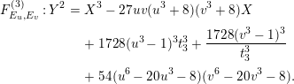 $$\begin{eqnarray}\displaystyle F_{E_{u},E_{v}}^{(3)}:Y^{2} & = & \displaystyle X^{3}-27uv(u^{3}+8)(v^{3}+8)X\nonumber\\ \displaystyle & & \displaystyle +\,1728(u^{3}-1)^{3}t_{3}^{3}+\frac{1728(v^{3}-1)^{3}}{t_{3}^{3}}\nonumber\\ \displaystyle & & \displaystyle +\,54(u^{6}-20u^{3}-8)(v^{6}-20v^{3}-8).\end{eqnarray}$$
Here, since
 $\unicode[STIX]{x1D6E5}_{E_{1}}=2^{12}\cdot 3^{9}(\unicode[STIX]{x1D707}^{3}-1)^{3}$
, and so forth, we scaled
$\unicode[STIX]{x1D6E5}_{E_{1}}=2^{12}\cdot 3^{9}(\unicode[STIX]{x1D707}^{3}-1)^{3}$
, and so forth, we scaled
 $X$
and
$X$
and
 $Y$
differently from (2.8); the difference is a Weierstrass transformation over
$Y$
differently from (2.8); the difference is a Weierstrass transformation over
 $\mathbb{Q}$
.
$\mathbb{Q}$
.
Let
 ${\mathcal{E}}_{u}\rightarrow \mathbb{P}_{u}^{1}$
and
${\mathcal{E}}_{u}\rightarrow \mathbb{P}_{u}^{1}$
and
 ${\mathcal{E}}_{v}\rightarrow \mathbb{P}_{v}^{1}$
be the elliptic modular surfaces associated with
${\mathcal{E}}_{v}\rightarrow \mathbb{P}_{v}^{1}$
be the elliptic modular surfaces associated with
 $E_{u}$
and
$E_{u}$
and
 $E_{v}$
, respectively. Also let
$E_{v}$
, respectively. Also let
 $G_{u}=\langle \unicode[STIX]{x1D703}_{u},\unicode[STIX]{x1D70C}_{u}\rangle$
and
$G_{u}=\langle \unicode[STIX]{x1D703}_{u},\unicode[STIX]{x1D70C}_{u}\rangle$
and
 $G_{v}=\langle \unicode[STIX]{x1D703}_{v},\unicode[STIX]{x1D70C}_{v}\rangle$
be groups of automorphisms of
$G_{v}=\langle \unicode[STIX]{x1D703}_{v},\unicode[STIX]{x1D70C}_{v}\rangle$
be groups of automorphisms of
 ${\mathcal{E}}_{u}$
and
${\mathcal{E}}_{u}$
and
 ${\mathcal{E}}_{v}$
described above, respectively. We consider (4.3) as the family of elliptic surfaces
${\mathcal{E}}_{v}$
described above, respectively. We consider (4.3) as the family of elliptic surfaces
 ${\mathcal{F}}_{E_{u},E_{v}}^{(3)}\rightarrow \mathbb{P}_{u}^{1}\times \mathbb{P}_{v}^{1}$
parametrized by
${\mathcal{F}}_{E_{u},E_{v}}^{(3)}\rightarrow \mathbb{P}_{u}^{1}\times \mathbb{P}_{v}^{1}$
parametrized by
 $u$
and
$u$
and
 $v$
. The total space is a fourfold.
$v$
. The total space is a fourfold.
Proposition 4.3. The actions of
 $G_{u}$
and
$G_{u}$
and
 $G_{v}$
induce the action
$G_{v}$
induce the action
 $\widetilde{\unicode[STIX]{x1D6F1}}$
on the fourfold
$\widetilde{\unicode[STIX]{x1D6F1}}$
on the fourfold
 ${\mathcal{F}}_{E_{u},E_{v}}^{(3)}$
given by the following formulas.
${\mathcal{F}}_{E_{u},E_{v}}^{(3)}$
given by the following formulas.
 $$\begin{eqnarray}\displaystyle & \displaystyle \widetilde{\unicode[STIX]{x1D6F1}}(\unicode[STIX]{x1D703}_{u}):(X,Y,t_{3},u,v)\mapsto (\unicode[STIX]{x1D714}^{2}X,Y,\unicode[STIX]{x1D714}t_{3},\unicode[STIX]{x1D714}u,v) & \displaystyle \nonumber\\ \displaystyle & \displaystyle \widetilde{\unicode[STIX]{x1D6F1}}(\unicode[STIX]{x1D703}_{v}):(X,Y,t_{3},u,v)\mapsto (\unicode[STIX]{x1D714}^{2}X,Y,\unicode[STIX]{x1D714}^{2}t_{3},u,\unicode[STIX]{x1D714}v), & \displaystyle \nonumber\\ \displaystyle & \displaystyle \widetilde{\unicode[STIX]{x1D6F1}}(\unicode[STIX]{x1D70C}_{u}):(X,Y,t_{3},u,v)\mapsto \left(\!\frac{(2\unicode[STIX]{x1D714}+1)^{2}}{(u-1)^{2}}X,\frac{(2\unicode[STIX]{x1D714}+1)^{3}}{(u-1)^{3}}Y,\frac{(u-1)^{2}}{(2\unicode[STIX]{x1D714}+1)^{2}}t_{3},\frac{u+2}{u-1},v\!\right)\!, & \displaystyle \nonumber\\ \displaystyle & \displaystyle \widetilde{\unicode[STIX]{x1D6F1}}(\unicode[STIX]{x1D70C}_{v}):(X,Y,t_{3},u,v)\mapsto \left(\!\frac{(2\unicode[STIX]{x1D714}+1)^{2}}{(v-1)^{2}}X,\frac{(2\unicode[STIX]{x1D714}+1)^{3}}{(v-1)^{3}}Y,\frac{(2\unicode[STIX]{x1D714}+1)^{2}}{(v-1)^{2}}t_{3},u,\frac{v+2}{v-1}\!\right)\!. & \displaystyle \nonumber\end{eqnarray}$$
Proof. Recall that
 $F^{(6)}$
is, by definition, birationally equivalent to
$F^{(6)}$
is, by definition, birationally equivalent to
 $$\begin{eqnarray}x_{2}^{3}+cx_{2}+d=t_{6}^{6}(x_{1}^{3}+ax_{1}+b),\end{eqnarray}$$
where
 $a,b,c,d$
are appropriate functions of
$a,b,c,d$
are appropriate functions of
 $u,v$
. (Note also that
$u,v$
. (Note also that
 $F^{(3)}$
is not birationally equivalent to
$F^{(3)}$
is not birationally equivalent to
 $x_{2}^{3}+cx_{2}+d=t_{3}^{3}(x_{1}^{3}+ax_{1}+b)$
, the latter being a rational surface.) The action on
$x_{2}^{3}+cx_{2}+d=t_{3}^{3}(x_{1}^{3}+ax_{1}+b)$
, the latter being a rational surface.) The action on
 ${\mathcal{E}}_{u}$
or
${\mathcal{E}}_{u}$
or
 ${\mathcal{E}}_{v}$
induces the action on
${\mathcal{E}}_{v}$
induces the action on
 $(X,Y,t_{6})$
through the change of variables (2.4). The change of variables also depends on the choice of the rational point
$(X,Y,t_{6})$
through the change of variables (2.4). The change of variables also depends on the choice of the rational point
 $(1:t_{6}^{2}:0)$
.
$(1:t_{6}^{2}:0)$
.
Since
 $\unicode[STIX]{x1D703}_{u}$
acts as
$\unicode[STIX]{x1D703}_{u}$
acts as
 $(x_{1},y_{1},u)\mapsto (\unicode[STIX]{x1D714}^{2}x_{1},y_{1},\unicode[STIX]{x1D714}u)$
, it stabilizes the equation
$(x_{1},y_{1},u)\mapsto (\unicode[STIX]{x1D714}^{2}x_{1},y_{1},\unicode[STIX]{x1D714}u)$
, it stabilizes the equation
 $x_{2}^{3}+cx_{2}+d=t_{6}^{6}(x_{1}^{3}+ax_{1}+b)$
, but it moves the rational point
$x_{2}^{3}+cx_{2}+d=t_{6}^{6}(x_{1}^{3}+ax_{1}+b)$
, but it moves the rational point
 $(1:t_{6}^{2}:0)$
to
$(1:t_{6}^{2}:0)$
to
 $(\unicode[STIX]{x1D714}^{2}:t_{6}^{2}:0)=\big(1:(\unicode[STIX]{x1D714}^{2}t_{6})^{2}:0\big)$
. Therefore,
$(\unicode[STIX]{x1D714}^{2}:t_{6}^{2}:0)=\big(1:(\unicode[STIX]{x1D714}^{2}t_{6})^{2}:0\big)$
. Therefore,
 $t_{6}\mapsto \unicode[STIX]{x1D714}^{2}t_{6}$
under this transformation. Using (2.4), we see that
$t_{6}\mapsto \unicode[STIX]{x1D714}^{2}t_{6}$
under this transformation. Using (2.4), we see that
 $X$
is mapped to
$X$
is mapped to
 $\unicode[STIX]{x1D714}^{2}X$
and
$\unicode[STIX]{x1D714}^{2}X$
and
 $Y$
remains invariant. Thus,
$Y$
remains invariant. Thus,
 $\unicode[STIX]{x1D703}_{u}$
acts as
$\unicode[STIX]{x1D703}_{u}$
acts as
 $(X,Y,t_{6},u,v)\mapsto (\unicode[STIX]{x1D714}^{2}X,Y,\unicode[STIX]{x1D714}^{2}t_{6},\unicode[STIX]{x1D714}u,v)$
on
$(X,Y,t_{6},u,v)\mapsto (\unicode[STIX]{x1D714}^{2}X,Y,\unicode[STIX]{x1D714}^{2}t_{6},\unicode[STIX]{x1D714}u,v)$
on
 ${\mathcal{F}}^{(6)}$
. This action descends to the above expression for
${\mathcal{F}}^{(6)}$
. This action descends to the above expression for
 $\widetilde{\unicode[STIX]{x1D6F1}}(\unicode[STIX]{x1D703}_{u})$
on
$\widetilde{\unicode[STIX]{x1D6F1}}(\unicode[STIX]{x1D703}_{u})$
on
 ${\mathcal{F}}_{E_{u},E_{v}}^{(3)}$
.
${\mathcal{F}}_{E_{u},E_{v}}^{(3)}$
.
As for
 $\unicode[STIX]{x1D70C}_{u}$
, the action
$\unicode[STIX]{x1D70C}_{u}$
, the action
 $$\begin{eqnarray}\displaystyle (x_{1},x_{2},t_{6},u,v)\mapsto \left(\frac{(2\unicode[STIX]{x1D714}+1)^{2}}{(u-1)^{2}}x_{1},x_{2},\frac{(u-1)}{(2\unicode[STIX]{x1D714}+1)}t_{6},\frac{(u+2)}{(u-1)},v\right) & & \displaystyle \nonumber\end{eqnarray}$$
stabilizes the equation, and by following the change of coordinates (2.4), we obtain the desired formula. Similarly, we obtain the expressions for
 $\unicode[STIX]{x1D703}_{v}$
and
$\unicode[STIX]{x1D703}_{v}$
and
 $\unicode[STIX]{x1D70C}_{v}$
.◻
$\unicode[STIX]{x1D70C}_{v}$
.◻
For clarity of notation, we will henceforth use just
 $\unicode[STIX]{x1D6FE}$
instead of
$\unicode[STIX]{x1D6FE}$
instead of
 $\unicode[STIX]{x1D70B}(\unicode[STIX]{x1D6FE}),\widetilde{\unicode[STIX]{x1D70B}}(\unicode[STIX]{x1D6FE}),\unicode[STIX]{x1D6F1}(\unicode[STIX]{x1D6FE}),\widetilde{\unicode[STIX]{x1D6F1}}(\unicode[STIX]{x1D6FE})$
, with the action being understood.
$\unicode[STIX]{x1D70B}(\unicode[STIX]{x1D6FE}),\widetilde{\unicode[STIX]{x1D70B}}(\unicode[STIX]{x1D6FE}),\unicode[STIX]{x1D6F1}(\unicode[STIX]{x1D6FE}),\widetilde{\unicode[STIX]{x1D6F1}}(\unicode[STIX]{x1D6FE})$
, with the action being understood.
Corollary 4.4. The group
 $G_{u}\times G_{v}$
acts on the group of sections
$G_{u}\times G_{v}$
acts on the group of sections
 $F_{E_{u},E_{v}}^{(3)}(\bar{k}(u,v)(t_{3}))$
. More precisely, if
$F_{E_{u},E_{v}}^{(3)}(\bar{k}(u,v)(t_{3}))$
. More precisely, if
 $\unicode[STIX]{x1D6FE}\in G_{u}\times G_{v}$
and
$\unicode[STIX]{x1D6FE}\in G_{u}\times G_{v}$
and
 $s\in F_{E_{u},E_{v}}^{(3)}(\bar{k}(u,v)(t_{3}))$
is given by
$s\in F_{E_{u},E_{v}}^{(3)}(\bar{k}(u,v)(t_{3}))$
is given by
 $X(t_{3},u,v)$
and
$X(t_{3},u,v)$
and
 $Y(t_{3},u,v)$
, then
$Y(t_{3},u,v)$
, then
 $\unicode[STIX]{x1D6FE}\cdot s$
is given by
$\unicode[STIX]{x1D6FE}\cdot s$
is given by
 $$\begin{eqnarray}\unicode[STIX]{x1D6FE}X\big(\unicode[STIX]{x1D6FE}^{-1}t_{3},\unicode[STIX]{x1D6FE}^{-1}u,\unicode[STIX]{x1D6FE}^{-1}v\big)\qquad \text{and}\qquad \unicode[STIX]{x1D6FE}Y\big(\unicode[STIX]{x1D6FE}^{-1}t_{3},\unicode[STIX]{x1D6FE}^{-1}u,\unicode[STIX]{x1D6FE}^{-1}v\big).\end{eqnarray}$$
From the action of
 $D_{6}$
on
$D_{6}$
on
 $F^{(6)}$
(see (2.5)), we see that
$F^{(6)}$
(see (2.5)), we see that
 $\langle \unicode[STIX]{x1D70E}^{2},\unicode[STIX]{x1D70F}\rangle \simeq D_{3}\simeq S_{3}$
acts on
$\langle \unicode[STIX]{x1D70E}^{2},\unicode[STIX]{x1D70F}\rangle \simeq D_{3}\simeq S_{3}$
acts on
 $F^{(3)}$
. We summarize the action on a section
$F^{(3)}$
. We summarize the action on a section
 $(X(t_{3},u,v),Y(t_{3},u,v))$
as follows.
$(X(t_{3},u,v),Y(t_{3},u,v))$
as follows.
 $$\begin{eqnarray}\displaystyle & \displaystyle \unicode[STIX]{x1D70E}^{2}\big(X(t_{3},u,v),Y(t_{3},u,v)\big)=\big(X(\unicode[STIX]{x1D714}^{2}t_{3},u,v),Y(\unicode[STIX]{x1D714}^{2}t_{3},u,v)\big) & \displaystyle \nonumber\\ \displaystyle & \unicode[STIX]{x1D70F}\big(X(t_{3},u,v),Y(t_{3},u,v)\big)=\big(X(\unicode[STIX]{x1D6FF}^{2}/t_{3},u,v),Y(\unicode[STIX]{x1D6FF}^{2}/t_{3},u,v)\big) & \displaystyle \nonumber\\ \displaystyle & \displaystyle \unicode[STIX]{x1D703}_{u}\big(X(t_{3},u,v),Y(t_{3},u,v)\big)=\big(\unicode[STIX]{x1D714}^{2}X(\unicode[STIX]{x1D714}^{2}t_{3},\unicode[STIX]{x1D714}^{2}u,v),Y(\unicode[STIX]{x1D714}^{2}t_{3},\unicode[STIX]{x1D714}^{2}u,v)\big) & \displaystyle \nonumber\\ \displaystyle & \displaystyle \unicode[STIX]{x1D703}_{v}\big(X(t_{3},u,v),Y(t_{3},u,v)\big)=\big(\unicode[STIX]{x1D714}^{2}X(\unicode[STIX]{x1D714}t_{3},u,\unicode[STIX]{x1D714}^{2}v),Y(\unicode[STIX]{x1D714}t_{3},u,\unicode[STIX]{x1D714}^{2}v)\big) & \displaystyle \nonumber\end{eqnarray}$$
 $$\begin{eqnarray}\displaystyle \unicode[STIX]{x1D70C}_{u}\big(X(t_{3},u,v),Y(t_{3},u,v)\big) & = & \displaystyle \left(\frac{(u-1)^{2}}{(2\unicode[STIX]{x1D714}+1)^{2}}X\Bigl(\frac{(u-1)^{2}}{(2\unicode[STIX]{x1D714}+1)^{2}}t_{3},\frac{u+2}{u-1},v\Bigr),\right.\nonumber\\ \displaystyle & & \displaystyle \left.-\,\frac{(u-1)^{3}}{(2\unicode[STIX]{x1D714}+1)^{3}}Y\Bigl(\frac{(u-1)^{2}}{(2\unicode[STIX]{x1D714}+1)^{2}}t_{3},\frac{u+2}{u-1},v\Bigr)\right)\nonumber\\ \displaystyle \unicode[STIX]{x1D70C}_{v}\big(X(t_{3},u,v),Y(t_{3},u,v)\big) & = & \displaystyle \left(\frac{(v-1)^{2}}{(2\unicode[STIX]{x1D714}+1)^{2}}X\Bigl(\frac{(2\unicode[STIX]{x1D714}+1)^{2}}{(v-1)^{2}}t_{3},u,\frac{v+2}{v-1}\Bigr),\right.\nonumber\\ \displaystyle & & \displaystyle \left.-\,\frac{(v-1)^{3}}{(2\unicode[STIX]{x1D714}+1)^{3}}Y\Bigl(\frac{(2\unicode[STIX]{x1D714}+1)^{2}}{(v-1)^{2}}t_{3},u,\frac{v+2}{v-1}\Bigr)\right).\nonumber\end{eqnarray}$$
We may expect that the orbit of a section by these automorphisms generates the whole Mordell–Weil group, and it turns out that it is the case. To show this we must find one section, and we will do this in the following subsections.
4.3 Computation of
$M(s_{3,0})$

As we modified the equation of
 $F^{(3)}$
from the one in Section 2, we also change the definition of
$F^{(3)}$
from the one in Section 2, we also change the definition of
 $s_{3,i}$
to
$s_{3,i}$
to
 $$\begin{eqnarray}s_{3,i}=4\Bigl((u^{3}-1)t_{3}+\frac{v^{3}-1}{\unicode[STIX]{x1D714}^{i}t_{3}}\Bigr).\end{eqnarray}$$
In what follows we denote
 $s_{3,0}$
simply by
$s_{3,0}$
simply by
 $s$
. Then, (4.3) becomes
$s$
. Then, (4.3) becomes
 $$\begin{eqnarray}\displaystyle R_{s}^{(3)}:Y^{2} & = & \displaystyle X^{3}-27uv(u^{3}+8)(v^{3}+8)X\nonumber\\ \displaystyle & & \displaystyle +\,27(s^{3}-48(u^{3}-1)(v^{3}-1)s\nonumber\\ \displaystyle & & \displaystyle +\,2(u^{6}-20u^{3}-8)(v^{6}-20v^{3}-8)).\end{eqnarray}$$
 $R_{s}^{(3)}$
is a rational elliptic surface over
$R_{s}^{(3)}$
is a rational elliptic surface over
 $k(u,v)$
that has a singular fiber of type I
$k(u,v)$
that has a singular fiber of type I
 $_{0}^{\ast }$
at
$_{0}^{\ast }$
at
 $s=\infty$
. As a consequence, its Mordell–Weil lattice is of type
$s=\infty$
. As a consequence, its Mordell–Weil lattice is of type
 $D_{4}^{\ast }$
(type
$D_{4}^{\ast }$
(type
 $\text{n}^{\circ }~9$
in the Oguiso–Shioda [Reference Oguiso and ShiodaOS] classification). The Mordell–Weil lattice of a rational elliptic surface is generated by the section of the form
$\text{n}^{\circ }~9$
in the Oguiso–Shioda [Reference Oguiso and ShiodaOS] classification). The Mordell–Weil lattice of a rational elliptic surface is generated by the section of the form
 $(c_{2}s^{2}+c_{1}s+c_{0},d_{3}s^{3}+d^{2}s^{2}+d_{1}s+d_{0})$
. An easy calculation shows that the fact that our elliptic surface has a singular fiber of type I
$(c_{2}s^{2}+c_{1}s+c_{0},d_{3}s^{3}+d^{2}s^{2}+d_{1}s+d_{0})$
. An easy calculation shows that the fact that our elliptic surface has a singular fiber of type I
 $_{0}^{\ast }$
at
$_{0}^{\ast }$
at
 $s=\infty$
implies
$s=\infty$
implies
 $c_{2}=d_{3}=d_{2}=0$
. Some further calculations show that we have a point
$c_{2}=d_{3}=d_{2}=0$
. Some further calculations show that we have a point
 $P_{0}$
given by
$P_{0}$
given by
 $$\begin{eqnarray}\displaystyle P_{0} & = & \displaystyle \Bigl(-3s-9(uv+2)^{2},\nonumber\\ \displaystyle & & \displaystyle \quad (2\unicode[STIX]{x1D714}+1)^{3}(3(uv+2)s+4(u^{3}-1)(v^{3}-1)+36(u^{2}v^{2}+uv+1))\Bigr).\nonumber\end{eqnarray}$$
The actions of
 $\unicode[STIX]{x1D703}_{u}$
and
$\unicode[STIX]{x1D703}_{u}$
and
 $\unicode[STIX]{x1D703}_{v}$
do not leave
$\unicode[STIX]{x1D703}_{v}$
do not leave
 $M(s_{3,0})=R_{s}^{(3)}(\overline{k}(s))$
invariant, but
$M(s_{3,0})=R_{s}^{(3)}(\overline{k}(s))$
invariant, but
 $\bar{\unicode[STIX]{x1D703}}_{u}:=\unicode[STIX]{x1D70E}^{4}\circ \unicode[STIX]{x1D703}_{u}$
and
$\bar{\unicode[STIX]{x1D703}}_{u}:=\unicode[STIX]{x1D70E}^{4}\circ \unicode[STIX]{x1D703}_{u}$
and
 $\bar{\unicode[STIX]{x1D703}}_{v}:=\unicode[STIX]{x1D70E}^{2}\circ \unicode[STIX]{x1D703}_{v}$
do. In fact, it is easily verified that the action of
$\bar{\unicode[STIX]{x1D703}}_{v}:=\unicode[STIX]{x1D70E}^{2}\circ \unicode[STIX]{x1D703}_{v}$
do. In fact, it is easily verified that the action of
 $\bar{\unicode[STIX]{x1D703}}_{u}$
and
$\bar{\unicode[STIX]{x1D703}}_{u}$
and
 $\bar{\unicode[STIX]{x1D703}}_{v}$
on
$\bar{\unicode[STIX]{x1D703}}_{v}$
on
 $F^{(3)}$
fix
$F^{(3)}$
fix
 $s$
. On the other hand,
$s$
. On the other hand,
 $\unicode[STIX]{x1D70C}_{u}$
and
$\unicode[STIX]{x1D70C}_{u}$
and
 $\unicode[STIX]{x1D70C}_{v}$
leave
$\unicode[STIX]{x1D70C}_{v}$
leave
 $M(s_{3,0})$
invariant; they take
$M(s_{3,0})$
invariant; they take
 $s$
to
$s$
to
 $(2\unicode[STIX]{x1D714}+1)^{2}/(u-1)^{2}s$
and
$(2\unicode[STIX]{x1D714}+1)^{2}/(u-1)^{2}s$
and
 $(2\unicode[STIX]{x1D714}+1)^{2}/(v-1)^{2}$
, respectively. The actions of
$(2\unicode[STIX]{x1D714}+1)^{2}/(v-1)^{2}$
, respectively. The actions of
 $\bar{\unicode[STIX]{x1D703}}_{u}$
,
$\bar{\unicode[STIX]{x1D703}}_{u}$
,
 $\bar{\unicode[STIX]{x1D703}}_{v}$
,
$\bar{\unicode[STIX]{x1D703}}_{v}$
,
 $\unicode[STIX]{x1D70C}_{u}$
and
$\unicode[STIX]{x1D70C}_{u}$
and
 $\unicode[STIX]{x1D70C}_{v}$
on
$\unicode[STIX]{x1D70C}_{v}$
on
 $M(s_{3,0})$
are given as follows.
$M(s_{3,0})$
are given as follows.
 $$\begin{eqnarray}\displaystyle \bar{\unicode[STIX]{x1D703}}_{u}\big(X(s,u,v),Y(s,u,v)\big) & = & \displaystyle \big(\unicode[STIX]{x1D714}^{2}X(s,\unicode[STIX]{x1D714}^{2}u,v),Y(s,\unicode[STIX]{x1D714}^{2}u,v)\big)\nonumber\\ \displaystyle \bar{\unicode[STIX]{x1D703}}_{v}\big(X(s,u,v),Y(s,u,v)\big) & = & \displaystyle \big(\unicode[STIX]{x1D714}^{2}X(s,u,\unicode[STIX]{x1D714}^{2}v),Y(s,u,\unicode[STIX]{x1D714}^{2}v)\big)\nonumber\\ \displaystyle \unicode[STIX]{x1D70C}_{u}\big(X(s,u,v),Y(s,u,v)\big) & = & \displaystyle \left(\frac{(u-1)^{2}}{(2\unicode[STIX]{x1D714}+1)^{2}}X\Bigl(\frac{(2\unicode[STIX]{x1D714}+1)^{2}}{(u-1)^{2}}s,\frac{u+2}{u-1},v\Bigr),\right.\nonumber\\ \displaystyle & & \displaystyle \quad \left.-\,\frac{(u-1)^{3}}{(2\unicode[STIX]{x1D714}+1)^{3}}Y\Bigl(\frac{(2\unicode[STIX]{x1D714}+1)^{2}}{(u-1)^{2}}s,\frac{u+2}{u-1},v\Bigr)\right)\nonumber\\ \displaystyle \unicode[STIX]{x1D70C}_{v}\big(X(s,u,v),Y(s,u,v)\big) & = & \displaystyle \left(\frac{(v-1)^{2}}{(2\unicode[STIX]{x1D714}+1)^{2}}X\Bigl(\frac{(2\unicode[STIX]{x1D714}+1)^{2}}{(v-1)^{2}}s,u,\frac{v+2}{v-1}\Bigr),\right.\nonumber\\ \displaystyle & & \displaystyle \quad \left.-\,\frac{(v-1)^{3}}{(2\unicode[STIX]{x1D714}+1)^{3}}Y\Bigl(\frac{(2\unicode[STIX]{x1D714}+1)^{2}}{(v-1)^{2}}s,u,\frac{v+2}{v-1}\Bigr)\right).\nonumber\end{eqnarray}$$
Proposition 4.5. The group of sections
 $$\begin{eqnarray}M(s_{3,0})=R_{s}^{(3)}(\bar{k}(s))\subset F_{E_{u},E_{v}}^{(3)}(\bar{k}(t_{3}))\end{eqnarray}$$
is invariant under the automorphisms
 $\bar{\unicode[STIX]{x1D703}}_{u}$
,
$\bar{\unicode[STIX]{x1D703}}_{u}$
,
 $\bar{\unicode[STIX]{x1D703}}_{v}$
,
$\bar{\unicode[STIX]{x1D703}}_{v}$
,
 $\unicode[STIX]{x1D70C}_{u}$
,
$\unicode[STIX]{x1D70C}_{u}$
,
 $\unicode[STIX]{x1D70C}_{v}$
. The group
$\unicode[STIX]{x1D70C}_{v}$
. The group
 $\langle \bar{\unicode[STIX]{x1D703}}_{u},\bar{\unicode[STIX]{x1D703}}_{v},\unicode[STIX]{x1D70C}_{u},\unicode[STIX]{x1D70C}_{v}\rangle$
acts on the lattice
$\langle \bar{\unicode[STIX]{x1D703}}_{u},\bar{\unicode[STIX]{x1D703}}_{v},\unicode[STIX]{x1D70C}_{u},\unicode[STIX]{x1D70C}_{v}\rangle$
acts on the lattice
 $M(s_{3,0})$
, and
$M(s_{3,0})$
, and
 $M(s_{3,0})$
is generated by
$M(s_{3,0})$
is generated by
 $$\begin{eqnarray}P_{0},\qquad \bar{\unicode[STIX]{x1D703}}_{u}(P_{0}),\qquad (\bar{\unicode[STIX]{x1D703}}_{u}\unicode[STIX]{x1D70C}_{u})(P_{0}),\qquad \text{and}\qquad (\unicode[STIX]{x1D70C}_{u}^{-1}\bar{\unicode[STIX]{x1D703}}_{u}\unicode[STIX]{x1D70C}_{u})(P_{0}).\end{eqnarray}$$
Furthermore, the height pairing matrix with respect to these sections is given by
 $$\begin{eqnarray}\frac{1}{2}\left(\begin{array}{@{}rrrr@{}}2 & -1 & -1 & -1\\ -1 & 2 & 0 & 0\\ -1 & 0 & 2 & 0\\ -1 & 0 & 0 & 2\end{array}\right).\end{eqnarray}$$
All the twenty-four sections of minimal height
 $1$
are obtained from
$1$
are obtained from
 $P_{0}$
by the automorphism group
$P_{0}$
by the automorphism group
 $\langle \bar{\unicode[STIX]{x1D703}}_{u},\unicode[STIX]{x1D70C}_{u}\rangle$
.
$\langle \bar{\unicode[STIX]{x1D703}}_{u},\unicode[STIX]{x1D70C}_{u}\rangle$
.
Proof. First of all, we verify that
 $s_{3,0}$
is invariant under the action of the group
$s_{3,0}$
is invariant under the action of the group
 $\langle \bar{\unicode[STIX]{x1D703}}_{u},\unicode[STIX]{x1D70C}_{u}\rangle$
. We then check that the order of the group
$\langle \bar{\unicode[STIX]{x1D703}}_{u},\unicode[STIX]{x1D70C}_{u}\rangle$
. We then check that the order of the group
 $\langle \bar{\unicode[STIX]{x1D703}}_{u},\unicode[STIX]{x1D70C}_{u}\rangle$
is
$\langle \bar{\unicode[STIX]{x1D703}}_{u},\unicode[STIX]{x1D70C}_{u}\rangle$
is
 $24$
. Then, by calculation, we verify that the orbit of
$24$
. Then, by calculation, we verify that the orbit of
 $P_{0}$
contains
$P_{0}$
contains
 $24$
different sections. We then choose four sections whose height matrix coincides with the desired form.◻
$24$
different sections. We then choose four sections whose height matrix coincides with the desired form.◻
Remark 4.6. The
 $X$
-coordinates of four sections above are as follows.
$X$
-coordinates of four sections above are as follows.
 $$\begin{eqnarray}\displaystyle X(P_{0}) & = & \displaystyle -3s-9(uv+2)^{2},\nonumber\\ \displaystyle X(\bar{\unicode[STIX]{x1D703}}_{u}(P_{0})) & = & \displaystyle -3\unicode[STIX]{x1D714}^{2}s-9(uv+2\unicode[STIX]{x1D714})^{2},\nonumber\\ \displaystyle X((\bar{\unicode[STIX]{x1D703}}_{u}\unicode[STIX]{x1D70C}_{u})(P_{0})) & = & \displaystyle -3\unicode[STIX]{x1D714}^{2}s+3(uv+2u+2\unicode[STIX]{x1D714}v-2\unicode[STIX]{x1D714})^{2},\nonumber\\ \displaystyle X((\unicode[STIX]{x1D70C}_{u}^{-1}\bar{\unicode[STIX]{x1D703}}_{u}\unicode[STIX]{x1D70C}_{u})(P_{0})) & = & \displaystyle -3\unicode[STIX]{x1D714}^{2}s+3(uv+2\unicode[STIX]{x1D714}^{2}u+2\unicode[STIX]{x1D714}^{2}v-2\unicode[STIX]{x1D714})^{2}.\nonumber\end{eqnarray}$$
The
 $Y$
-coordinates are a little more complicated and we omit them here.Footnote
2
$Y$
-coordinates are a little more complicated and we omit them here.Footnote
2
4.4
$F^{(3)}(\overline{k}(t_{3}))$
in the generic case

If we consider
 $E_{u}$
and
$E_{u}$
and
 $E_{v}$
as universal curves with independent variables
$E_{v}$
as universal curves with independent variables
 $u$
and
$u$
and
 $v$
, they are not isogenous curves. Looking at the diagram at the end of Section 2,
$v$
, they are not isogenous curves. Looking at the diagram at the end of Section 2,
 $F^{(3)}(\bar{k}(t_{3}))$
contains four sublattices,
$F^{(3)}(\bar{k}(t_{3}))$
contains four sublattices,
 $F^{(1)}(\bar{k}(t_{1}))$
,
$F^{(1)}(\bar{k}(t_{1}))$
,
 $M(s_{3,0})$
,
$M(s_{3,0})$
,
 $M(s_{3,1})$
and
$M(s_{3,1})$
and
 $M(s_{3,2})$
. In our case
$M(s_{3,2})$
. In our case
 $F^{(1)}(\bar{k}(t_{1}))$
is trivial.
$F^{(1)}(\bar{k}(t_{1}))$
is trivial.
Lemma 4.7. The lattice
 $M(s_{3,1})$
is the image of
$M(s_{3,1})$
is the image of
 $M(s_{3,0})$
by the automorphism
$M(s_{3,0})$
by the automorphism
 $\unicode[STIX]{x1D70E}^{2}$
of
$\unicode[STIX]{x1D70E}^{2}$
of
 $F^{(3)}(\bar{k}(t_{3}))$
, and
$F^{(3)}(\bar{k}(t_{3}))$
, and
 $M(s_{3,2})$
is the image of
$M(s_{3,2})$
is the image of
 $M(s_{3,0})$
by
$M(s_{3,0})$
by
 $\unicode[STIX]{x1D70E}^{4}$
. In particular
$\unicode[STIX]{x1D70E}^{4}$
. In particular
 $M(s_{3,0})$
,
$M(s_{3,0})$
,
 $M(s_{3,1})$
and
$M(s_{3,1})$
and
 $M(s_{3,2})$
are all isomorphic.
$M(s_{3,2})$
are all isomorphic.
Proof. From the identity
 $$\begin{eqnarray}\displaystyle s^{3}-3s & = & \displaystyle \Bigl(t+\frac{1}{t}\Bigr)^{3}-3\Bigl(t+\frac{1}{t}\Bigr)=t^{3}+\frac{1}{t^{3}}\nonumber\\ \displaystyle & = & \displaystyle t^{3}+\frac{1}{(\unicode[STIX]{x1D714}t)^{3}}=\Bigl(t+\frac{1}{\unicode[STIX]{x1D714}t}\Bigr)^{3}-3\unicode[STIX]{x1D714}^{2}\Bigl(t+\frac{1}{\unicode[STIX]{x1D714}t}\Bigr)=s_{1}^{3}-3\unicode[STIX]{x1D714}^{2}s_{1},\nonumber\end{eqnarray}$$
we see that the lattice
 $M(s_{3,1})$
is the Mordell–Weil lattice of the elliptic curve given by the equation obtained by replacing
$M(s_{3,1})$
is the Mordell–Weil lattice of the elliptic curve given by the equation obtained by replacing
 $s$
by
$s$
by
 $\unicode[STIX]{x1D714}^{2}s_{3,1}$
in (4.4). The assertion is now clear from
$\unicode[STIX]{x1D714}^{2}s_{3,1}$
in (4.4). The assertion is now clear from
 $$\begin{eqnarray}s_{3,1}=4\unicode[STIX]{x1D714}\left((u^{3}-1)\unicode[STIX]{x1D714}^{2}t_{3}+\frac{(v^{3}-1)}{\unicode[STIX]{x1D714}^{2}t_{3}}\right)=\unicode[STIX]{x1D714}\unicode[STIX]{x1D70E}^{2}(s_{3,0}).\end{eqnarray}$$
Similarly for
 $M(s_{3,2})$
.◻
$M(s_{3,2})$
.◻
Theorem 4.8. Let
 $u,v\in \overline{k}$
be such that
$u,v\in \overline{k}$
be such that
 $E_{u}$
and
$E_{u}$
and
 $E_{v}$
are not isogenous. The Mordell–Weil group
$E_{v}$
are not isogenous. The Mordell–Weil group
 $F_{E_{u},E_{v}}^{(3)}(\bar{k}(t_{3}))$
for the elliptic curve
$F_{E_{u},E_{v}}^{(3)}(\bar{k}(t_{3}))$
for the elliptic curve
 $F_{E_{u},E_{v}}^{(3)}$
over
$F_{E_{u},E_{v}}^{(3)}$
over
 $k(u,v)$
defined by (4.3) are generated by
$k(u,v)$
defined by (4.3) are generated by
 $M(s_{3,0})$
and
$M(s_{3,0})$
and
 $M(s_{3,1})$
. As a lattice,
$M(s_{3,1})$
. As a lattice,
 $F_{E_{u},E_{v}}^{(3)}(\bar{k}(t_{3}))$
is generated by
$F_{E_{u},E_{v}}^{(3)}(\bar{k}(t_{3}))$
is generated by
 $$\begin{eqnarray}\displaystyle & \displaystyle (\unicode[STIX]{x1D70C}_{u}^{-1}\unicode[STIX]{x1D703}_{u}\unicode[STIX]{x1D70C}_{u})(P_{0}),\qquad (\unicode[STIX]{x1D703}_{u}\unicode[STIX]{x1D70C}_{u})(P_{0}),\qquad \unicode[STIX]{x1D703}_{u}(P_{0}),\qquad P_{0}, & \displaystyle \nonumber\\ \displaystyle & \displaystyle \unicode[STIX]{x1D70E}^{2}(P_{0}),\qquad (\unicode[STIX]{x1D70E}^{2}\unicode[STIX]{x1D703}_{u})(P_{0}),\qquad (\unicode[STIX]{x1D70E}^{2}\unicode[STIX]{x1D703}_{u}\unicode[STIX]{x1D70C}_{u})(P_{0}),\qquad \text{and}\qquad (\unicode[STIX]{x1D70E}^{2}\unicode[STIX]{x1D70C}_{u}^{-1}\unicode[STIX]{x1D703}_{u}\unicode[STIX]{x1D70C}_{u})(P_{0}) & \displaystyle \nonumber\end{eqnarray}$$
with the height pairing matrix
 $$\begin{eqnarray}\frac{1}{2}\left(\begin{array}{@{}rrrrrrrr@{}}4 & 0 & 0 & 1 & -2 & 0 & 0 & -2\\ 0 & 4 & 0 & 1 & -2 & 0 & -2 & 0\\ 0 & 0 & 4 & 1 & -2 & -2 & 0 & 0\\ 1 & 1 & 1 & 4 & -2 & 1 & 1 & 1\\ -2 & -2 & -2 & -2 & 4 & 1 & 1 & 1\\ 0 & 0 & -2 & 1 & 1 & 4 & 0 & 0\\ 0 & -2 & 0 & 1 & 1 & 0 & 4 & 0\\ -2 & 0 & 0 & 1 & 1 & 0 & 0 & 4\end{array}\right).\end{eqnarray}$$
Proof. We calculate the height pairing matrix with respect to the basis of
 $M(s_{3,0})$
in Proposition 4.5 together with it image under
$M(s_{3,0})$
in Proposition 4.5 together with it image under
 $\unicode[STIX]{x1D70E}^{2}$
, and verify that its determinant equals
$\unicode[STIX]{x1D70E}^{2}$
, and verify that its determinant equals
 $3^{4}/2^{4}$
, which coincides with the value given in [Reference ShiodaSh7].◻
$3^{4}/2^{4}$
, which coincides with the value given in [Reference ShiodaSh7].◻
Remark 4.9. The
 $x$
- and
$x$
- and
 $y$
-coordinates for this basis of sections may be easily computed from the group action, starting with
$y$
-coordinates for this basis of sections may be easily computed from the group action, starting with
 $P_{0}$
. We do not list them here for brevity, but they may be found in the auxiliary files. The same holds for any complicated or lengthy expressions suppressed in the body of the text.
$P_{0}$
. We do not list them here for brevity, but they may be found in the auxiliary files. The same holds for any complicated or lengthy expressions suppressed in the body of the text.
Corollary 4.10. Let
 $E_{1}$
and
$E_{1}$
and
 $E_{2}$
be elliptic curves over
$E_{2}$
be elliptic curves over
 $k$
. Suppose
$k$
. Suppose
 $E_{1}$
and
$E_{1}$
and
 $E_{2}$
are not isogenous. Then, the Mordell–Weil lattice
$E_{2}$
are not isogenous. Then, the Mordell–Weil lattice
 $F_{E_{1},E_{2}}^{(3)}(\bar{k}(t_{3}))$
is defined over
$F_{E_{1},E_{2}}^{(3)}(\bar{k}(t_{3}))$
is defined over
 $k(E_{1}[3],E_{2}[3])$
, the field over which all the
$k(E_{1}[3],E_{2}[3])$
, the field over which all the
 $3$
-torsion points of
$3$
-torsion points of
 $E_{1}$
and
$E_{1}$
and
 $E_{2}$
are defined.
$E_{2}$
are defined.
Proof. Over the field
 $K=k(E_{1}[3],E_{2}[3])$
,
$K=k(E_{1}[3],E_{2}[3])$
,
 $E_{1}$
and
$E_{1}$
and
 $E_{2}$
are isomorphic to
$E_{2}$
are isomorphic to
 $E_{u}$
and
$E_{u}$
and
 $E_{v}$
for suitable choices of
$E_{v}$
for suitable choices of
 $u$
and
$u$
and
 $v$
, respectively. By Theorem 4.8, the Mordell–Weil lattice
$v$
, respectively. By Theorem 4.8, the Mordell–Weil lattice
 $F_{E_{u},E_{v}}^{(3)}(\bar{k}(t_{3}))$
is defined over
$F_{E_{u},E_{v}}^{(3)}(\bar{k}(t_{3}))$
is defined over
 $K(\unicode[STIX]{x1D714})$
, but
$K(\unicode[STIX]{x1D714})$
, but
 $\unicode[STIX]{x1D714}$
is contained in
$\unicode[STIX]{x1D714}$
is contained in
 $K$
by the Weil pairing. Thus,
$K$
by the Weil pairing. Thus,
 $F_{E_{1},E_{2}}^{(3)}(\bar{k}(t_{3}))$
is defined over
$F_{E_{1},E_{2}}^{(3)}(\bar{k}(t_{3}))$
is defined over
 $K$
.◻
$K$
.◻
5 Mordell–Weil group of
$F^{(4)}$

5.1 Elliptic modular surface associated with
$\unicode[STIX]{x1D6E4}(4)$

The elliptic modular surface over the modular curve
 $X(4)$
is given by
$X(4)$
is given by
 $$\begin{eqnarray}E_{\unicode[STIX]{x1D70E}}:y^{2}=x(x+(\unicode[STIX]{x1D70E}^{2}+1)^{2})(x+(\unicode[STIX]{x1D70E}^{2}-1)^{2})\end{eqnarray}$$
(cf. [Reference ShiodaSh1]). The subgroup of
 $4$
-torsion points are generated by
$4$
-torsion points are generated by
 $$\begin{eqnarray}(-\unicode[STIX]{x1D70E}^{4}+1,2\unicode[STIX]{x1D70E}^{4}-2)\qquad \text{and}\qquad (-(\unicode[STIX]{x1D70E}^{2}-1)(\unicode[STIX]{x1D70E}+i)^{2},-2\unicode[STIX]{x1D70E}(\unicode[STIX]{x1D70E}^{2}-1)(\unicode[STIX]{x1D70E}+i)^{2}),\end{eqnarray}$$
where
 $i=\sqrt{-1}$
. The
$i=\sqrt{-1}$
. The
 $j$
-invariant of (5.1) is given by
$j$
-invariant of (5.1) is given by
 $$\begin{eqnarray}j=\frac{16(\unicode[STIX]{x1D70E}^{8}+14\unicode[STIX]{x1D70E}^{4}+1)^{3}}{\unicode[STIX]{x1D70E}^{4}(\unicode[STIX]{x1D70E}^{4}-1)^{4}}.\end{eqnarray}$$
Let
 $$\begin{eqnarray}\unicode[STIX]{x1D703}=\left(\begin{array}{@{}cc@{}}1 & 1\\ 0 & 1\end{array}\right)\qquad \text{and}\qquad \unicode[STIX]{x1D70C}=\left(\begin{array}{@{}cc@{}}0 & 1\\ -1 & 0\end{array}\right)\end{eqnarray}$$
be generators for
 $G=\operatorname{SL}_{2}(\mathbb{Z}/4\mathbb{Z})$
. Consider the following representation
$G=\operatorname{SL}_{2}(\mathbb{Z}/4\mathbb{Z})$
. Consider the following representation
 $\unicode[STIX]{x1D70B}$
of
$\unicode[STIX]{x1D70B}$
of
 $G$
on the projective line
$G$
on the projective line
 $\mathbb{P}_{\unicode[STIX]{x1D70E}}^{1}$
by fractional linear transformations, which factors through
$\mathbb{P}_{\unicode[STIX]{x1D70E}}^{1}$
by fractional linear transformations, which factors through
 $\operatorname{PSL}_{2}(\mathbb{Z}/4\mathbb{Z})$
.
$\operatorname{PSL}_{2}(\mathbb{Z}/4\mathbb{Z})$
.
 $$\begin{eqnarray}\unicode[STIX]{x1D70B}(\unicode[STIX]{x1D703}):\unicode[STIX]{x1D70E}\mapsto i\unicode[STIX]{x1D70E},\qquad \unicode[STIX]{x1D70B}(\unicode[STIX]{x1D70C}):\unicode[STIX]{x1D70E}\mapsto \frac{\unicode[STIX]{x1D70E}-2}{\unicode[STIX]{x1D70E}+1}.\end{eqnarray}$$
The
 $j$
-invariant is invariant under the action of
$j$
-invariant is invariant under the action of
 $\unicode[STIX]{x1D70B}(\operatorname{SL}_{2}(\mathbb{Z}/4\mathbb{Z}))$
.
$\unicode[STIX]{x1D70B}(\operatorname{SL}_{2}(\mathbb{Z}/4\mathbb{Z}))$
.
We take two copies of the elliptic modular surface (5.1):
 $$\begin{eqnarray}\displaystyle E_{u}:y_{1}^{2} & = & \displaystyle x_{1}(x_{1}+(u^{2}+1)^{2})(x_{1}+(u^{2}-1)^{2}),\nonumber\\ \displaystyle E_{v}:y_{2}^{2} & = & \displaystyle x_{2}(x_{2}+(v^{2}+1)^{2})(x_{2}+(v^{2}-1)^{2}).\nonumber\end{eqnarray}$$
We then obtain
 $F_{E_{u},E_{v}}^{(4)}$
:
$F_{E_{u},E_{v}}^{(4)}$
:
 $$\begin{eqnarray}\displaystyle F_{E_{u},E_{v}}^{(4)}:Y^{2} & = & \displaystyle X^{3}-27(u^{8}+14u^{4}+1)(v^{8}+14v^{4}+1)X\nonumber\\ \displaystyle & & \displaystyle +\,54\Bigl(54u^{4}(u^{4}-1)^{4}t^{4}+\frac{54v^{4}(v^{4}-1)^{4}}{t^{4}}\nonumber\\ \displaystyle & & \displaystyle +\,(u^{12}-33u^{8}-33u^{4}+1)(v^{12}-33v^{8}-33v^{4}+1)\Bigr).\end{eqnarray}$$
5.2 Rational elliptic surfaces
As before we set
 $$\begin{eqnarray}s_{j}=i^{j}u(u^{4}-1)t+\frac{v(v^{4}-1)}{t}.\end{eqnarray}$$
where
 $i=\sqrt{-1}$
. Then we may write the equation of
$i=\sqrt{-1}$
. Then we may write the equation of
 $F^{(4)}$
as
$F^{(4)}$
as
 $$\begin{eqnarray}R_{s_{j}}^{(4)}:Y^{2}=X^{3}-AX+4(s_{j}^{4}-4i^{j}Bs_{j}^{2}+2i^{2j}B^{2})+C,\end{eqnarray}$$
where
 $$\begin{eqnarray}\left\{\begin{array}{@{}l@{}}A=27(u^{8}+14u^{4}+1)(v^{8}+14v^{4}+1)\\ B=uv(u^{4}-1)(v^{4}-1)\\ C=54(u^{12}-33u^{8}-33u^{4}+1)(v^{12}-33v^{8}-33v^{4}+1).\end{array}\right.\end{eqnarray}$$
This is a rational elliptic surface over
 $\mathbb{P}_{s_{j}}^{1}$
, with a
$\mathbb{P}_{s_{j}}^{1}$
, with a
 $\text{IV}$
fiber over
$\text{IV}$
fiber over
 $s_{j}=\infty$
. Generically, this is the only reducible fiber, and the Mordell–Weil lattice is therefore
$s_{j}=\infty$
. Generically, this is the only reducible fiber, and the Mordell–Weil lattice is therefore
 $E_{6}^{\ast }$
. To describe the sections, note that it suffices to do so for
$E_{6}^{\ast }$
. To describe the sections, note that it suffices to do so for
 $R_{s_{0}}^{(4)}$
, since
$R_{s_{0}}^{(4)}$
, since
 $\big(X(u,v,s_{0}),Y(u,v,s_{0})\big)$
is a section of
$\big(X(u,v,s_{0}),Y(u,v,s_{0})\big)$
is a section of
 $R_{s_{0}}^{(4)}$
if and only if
$R_{s_{0}}^{(4)}$
if and only if
 $\big(X(i^{j}u,v,s_{i}),Y(i^{j}u,v,s_{i})\big)$
is a section of
$\big(X(i^{j}u,v,s_{i}),Y(i^{j}u,v,s_{i})\big)$
is a section of
 $R_{s_{j}}^{(4)}$
.
$R_{s_{j}}^{(4)}$
.
There are fifty-four sections of
 $R_{s_{0}}^{(4)}$
of minimal height, with twenty-seven sections intersecting each non-identity component of the
$R_{s_{0}}^{(4)}$
of minimal height, with twenty-seven sections intersecting each non-identity component of the
 $\text{IV}$
fiber.
$\text{IV}$
fiber.
To solve for the sections intersecting one of these, we set
 $$\begin{eqnarray}X=x_{0}+x_{1}s,\qquad Y=y_{0}+y_{1}s+54s^{2},\end{eqnarray}$$
(where we have written
 $s=s_{0}$
for ease of notation) and substitute into the Weierstrass equation. It is then easy to solve for the remaining coefficients. We obtain a basis of sections; we list the
$s=s_{0}$
for ease of notation) and substitute into the Weierstrass equation. It is then easy to solve for the remaining coefficients. We obtain a basis of sections; we list the
 $x$
-coordinates here for brevity. (The full sections may be found in the auxiliary files).
$x$
-coordinates here for brevity. (The full sections may be found in the auxiliary files).
 $$\begin{eqnarray}\displaystyle x(P_{1}) & = & \displaystyle -18(1+i)(uv+i)s\nonumber\\ \displaystyle & & \displaystyle -\,3(5u^{4}v^{4}-u^{4}-v^{4}+24iu^{3}v^{3}-24u^{2}v^{2}-24iuv+5),\nonumber\\ \displaystyle x(P_{2}) & = & \displaystyle 18(1+i)(uv+i)s\nonumber\\ \displaystyle & & \displaystyle -\,3(5u^{4}v^{4}-u^{4}-v^{4}+24iu^{3}v^{3}-24u^{2}v^{2}-24iuv+5),\nonumber\\ \displaystyle x(P_{3}) & = & \displaystyle 18(1-i)(uv-i)s\nonumber\\ \displaystyle & & \displaystyle -\,3(5u^{4}v^{4}-u^{4}-v^{4}-24iu^{3}v^{3}-24u^{2}v^{2}+24iuv+5),\nonumber\\ \displaystyle x(P_{4}) & = & \displaystyle 18(1-i)(u+iv)s\nonumber\\ \displaystyle & & \displaystyle +\,3(u^{4}v^{4}-5u^{4}-5v^{4}-24iu^{3}v+24u^{2}v^{2}+24iuv^{3}+1),\nonumber\\ \displaystyle x(P_{5}) & = & \displaystyle -18(1+i)(u-iv)s\nonumber\\ \displaystyle & & \displaystyle +\,3(u^{4}v^{4}-5u^{4}-5v^{4}+24iu^{3}v+24u^{2}v^{2}-24iuv^{3}+1),\nonumber\\ \displaystyle x(P_{6}) & = & \displaystyle 3(u^{4}v^{4}+u^{4}+v^{4}+6u^{4}v^{2}+6u^{2}v^{4}-12u^{2}v^{2}+6u^{2}+6v^{2}+1).\nonumber\end{eqnarray}$$
5.3 The Mordell–Weil group in the generic case
Let
 $P_{1},\ldots ,P_{6}$
be the sections obtained from
$P_{1},\ldots ,P_{6}$
be the sections obtained from
 $R_{s_{0}}^{(4)}$
, and
$R_{s_{0}}^{(4)}$
, and
 $P_{1}^{\prime },\ldots ,P_{6}^{\prime }$
the corresponding sections from
$P_{1}^{\prime },\ldots ,P_{6}^{\prime }$
the corresponding sections from
 $R_{s_{1}}^{(4)}$
(obtained by substituting
$R_{s_{1}}^{(4)}$
(obtained by substituting
 $iu$
for
$iu$
for
 $u$
in
$u$
in
 $P_{i}$
). Together, they do not quite span the whole Mordell–Weil lattice of
$P_{i}$
). Together, they do not quite span the whole Mordell–Weil lattice of
 $F^{(4)}$
. We define
$F^{(4)}$
. We define
 $$\begin{eqnarray}\displaystyle Q_{1} & = & \displaystyle -(P_{1}-P_{3}+P_{4}-P_{5}+P_{6})/2,\nonumber\\ \displaystyle Q_{1}^{\prime } & = & \displaystyle -(P_{1}^{\prime }-P_{3}^{\prime }+P_{4}^{\prime }-P_{5}^{\prime }+P_{6}^{\prime })/2;\nonumber\end{eqnarray}$$
expressions for these sections may be obtained from the computer files. Note that they are well defined by the equation above, since
 $\operatorname{MW}(F^{(4)})$
is torsion-free by Theorem 2.5.
$\operatorname{MW}(F^{(4)})$
is torsion-free by Theorem 2.5.
Theorem 5.1. Let
 $u,v\in \overline{k}$
be such that
$u,v\in \overline{k}$
be such that
 $E_{u}$
and
$E_{u}$
and
 $E_{v}$
are not isogenous. The sections
$E_{v}$
are not isogenous. The sections
 $P_{1},\ldots ,P_{5},Q_{1},P_{1}^{\prime },\ldots ,P_{5}^{\prime },Q_{1}^{\prime }$
form a basis of the Mordell–Weil lattice
$P_{1},\ldots ,P_{5},Q_{1},P_{1}^{\prime },\ldots ,P_{5}^{\prime },Q_{1}^{\prime }$
form a basis of the Mordell–Weil lattice
 $F_{E_{u},E_{v}}^{(4)}(\overline{k}(t_{4}))$
.
$F_{E_{u},E_{v}}^{(4)}(\overline{k}(t_{4}))$
.
Proof. The height pairing matrix of these sections has discriminant
 $4^{4}/3^{2}$
, which is the discriminant of the Mordell–Weil lattice in the generic case.◻
$4^{4}/3^{2}$
, which is the discriminant of the Mordell–Weil lattice in the generic case.◻
Corollary 5.2. Let
 $E_{1}$
and
$E_{1}$
and
 $E_{2}$
be elliptic curves over
$E_{2}$
be elliptic curves over
 $k$
. Suppose
$k$
. Suppose
 $E_{1}$
and
$E_{1}$
and
 $E_{2}$
are not isogenous. Then, the Mordell–Weil lattice
$E_{2}$
are not isogenous. Then, the Mordell–Weil lattice
 $F_{E_{1},E_{2}}^{(4)}(\bar{k}(t_{4}))$
is defined over
$F_{E_{1},E_{2}}^{(4)}(\bar{k}(t_{4}))$
is defined over
 $k(E_{1}[4],E_{2}[4])$
, the field over which all the
$k(E_{1}[4],E_{2}[4])$
, the field over which all the
 $4$
-torsion points of
$4$
-torsion points of
 $E_{1}$
and
$E_{1}$
and
 $E_{2}$
are defined.
$E_{2}$
are defined.
5.4
$F^{(4)}$
as a quartic surface

The minimal nonsingular model of
 $F_{E_{u},E_{v}}^{(4)}$
is isomorphic to the quartic surface defined by
$F_{E_{u},E_{v}}^{(4)}$
is isomorphic to the quartic surface defined by
 $$\begin{eqnarray}\displaystyle & & \displaystyle S_{4}:ZW(Z+(v^{2}+1)^{2}W)(Z+(v^{2}-1)^{2}W)\nonumber\\ \displaystyle & & \displaystyle \qquad =XY(X+(u^{2}+1)^{2}Y)(X+(u^{2}-1)^{2}Y).\end{eqnarray}$$
 $F_{E_{u},E_{v}}^{(4)}$
corresponds to the elliptic fibration on
$F_{E_{u},E_{v}}^{(4)}$
corresponds to the elliptic fibration on
 $S_{4}$
defined by the elliptic parameter
$S_{4}$
defined by the elliptic parameter
 $t_{4}=Y/W$
. Generically, this quartic surface contains sixteen lines (cf. [Reference SegreSe, Reference InoseI1, Reference KuwataKw1]). They are obtained as the intersection of one of the four planes
$t_{4}=Y/W$
. Generically, this quartic surface contains sixteen lines (cf. [Reference SegreSe, Reference InoseI1, Reference KuwataKw1]). They are obtained as the intersection of one of the four planes
 $$\begin{eqnarray}X=0,\qquad Y=0,\qquad X+(u^{2}+1)^{2}Y=0,\qquad X+(u^{2}-1)^{2}Y=0\end{eqnarray}$$
and one of the four planes
 $$\begin{eqnarray}Z=0,\qquad W=0,\qquad Z+(v^{2}+1)^{2}W=0,\qquad Z+(v^{2}-1)^{2}W=0.\end{eqnarray}$$
We identify
 $S_{4}$
and
$S_{4}$
and
 $F^{(4)}$
by choosing
$F^{(4)}$
by choosing
 $X=Z=0$
as the
$X=Z=0$
as the
 $0$
-section. Let
$0$
-section. Let
 $L_{1},\ldots ,L_{4}$
be four lines defined by
$L_{1},\ldots ,L_{4}$
be four lines defined by
 $$\begin{eqnarray}\displaystyle & \displaystyle L_{1}:X+(u^{2}+1)^{2}Y=Z+(v^{2}+1)^{2}W=0, & \displaystyle \nonumber\\ \displaystyle & \displaystyle L_{2}:X+(u^{2}-1)^{2}Y=Z+(v^{2}-1)^{2}W=0, & \displaystyle \nonumber\\ \displaystyle & \displaystyle L_{3}:X+(u^{2}+1)^{2}Y=Z+(v^{2}-1)^{2}W=0, & \displaystyle \nonumber\\ \displaystyle & \displaystyle L_{4}:X+(u^{2}-1)^{2}Y=Z+(v^{2}+1)^{2}W=0. & \displaystyle \nonumber\end{eqnarray}$$
By an abuse of notation, we also denote by
 $L_{i}$
the corresponding section of
$L_{i}$
the corresponding section of
 $F_{E_{u},E_{v}}^{(4)}$
.
$F_{E_{u},E_{v}}^{(4)}$
.
 $S_{4}$
may be considered as a family of the intersection of two quadrics. Namely, consider the map
$S_{4}$
may be considered as a family of the intersection of two quadrics. Namely, consider the map
 $S_{4}\rightarrow \mathbb{P}^{1}$
given by
$S_{4}\rightarrow \mathbb{P}^{1}$
given by
 $$\begin{eqnarray}\unicode[STIX]{x1D708}:(X:Y:Z:W)\mapsto \big(XY+(u^{2}+1)Y^{2}:ZW\big).\end{eqnarray}$$
Over the point
 $(p:q)\in \mathbb{P}^{1}$
, the fiber of
$(p:q)\in \mathbb{P}^{1}$
, the fiber of
 $\unicode[STIX]{x1D708}$
is the intersection of two quadrics
$\unicode[STIX]{x1D708}$
is the intersection of two quadrics
 $$\begin{eqnarray}\left\{\begin{array}{@{}l@{}}rZW=Y(X+(u^{2}+1)^{2}Y),\\ (Z+(v^{2}+1)^{2}W)(Z+(v^{2}-1)^{2}W)=rX(X+(u^{2}-1)^{2}Y),\end{array}\right.\end{eqnarray}$$
where
 $r=p/q$
. The intersection is a curve of genus 1 for each
$r=p/q$
. The intersection is a curve of genus 1 for each
 $r$
, except the following eight values:
$r$
, except the following eight values:
 $$\begin{eqnarray}r=\frac{\pm 2i}{(u+1)^{2}},\qquad \frac{\pm 2i}{(u-1)^{2}},\qquad \frac{\pm 2iv^{2}}{(u+1)^{2}},\qquad \frac{\pm 2iv^{2}}{(u-1)^{2}}.\end{eqnarray}$$
At each of these values of
 $r$
, the intersection degenerates and becomes a union of two plane conics.
$r$
, the intersection degenerates and becomes a union of two plane conics.
Let
 $R_{1},\ldots ,R_{4}$
be one of the plane conics at each of the values
$R_{1},\ldots ,R_{4}$
be one of the plane conics at each of the values
 $$\begin{eqnarray}r=2i/(u+1)^{2},\qquad -2i/(u+1)^{2},\qquad 2i/(u-1)^{2},\qquad 2iv^{2}/(u-1)^{2},\end{eqnarray}$$
respectively. Similarly, in the family
 $$\begin{eqnarray}\left\{\begin{array}{@{}l@{}}rZ(Z+(v^{2}-1)^{2}W)=(X+(u^{2}+1)^{2}Y)(X+(u^{2}-1)^{2}Y),\\ W(Z+(v^{2}+1)^{2}W)=rXY,\end{array}\right.\end{eqnarray}$$
let
 $R_{5},R_{6}$
be one of the conics at the value
$R_{5},R_{6}$
be one of the conics at the value
 $r=\pm 2i/(v+1)^{2}$
, and let
$r=\pm 2i/(v+1)^{2}$
, and let
 $R_{7}$
be one of the conics at
$R_{7}$
be one of the conics at
 $r=(u+1)^{2}/(v+1)^{2}$
in the family
$r=(u+1)^{2}/(v+1)^{2}$
in the family
 $$\begin{eqnarray}\left\{\begin{array}{@{}l@{}}rZ(Z+(v^{2}-1)^{2}W)=X(X+(u^{2}-1)^{2}Y),\\ W(Z+(v^{2}+1)^{2}W)=rY(X+(u^{2}+1)^{2}Y).\end{array}\right.\end{eqnarray}$$
Explicit choices for
 $R_{1},\ldots ,R_{7}$
are made in the computer files. Finally, let
$R_{1},\ldots ,R_{7}$
are made in the computer files. Finally, let
 $R_{8}$
be the section obtained by letting
$R_{8}$
be the section obtained by letting
 $u\mapsto iu$
in
$u\mapsto iu$
in
 $R_{1}$
.
$R_{1}$
.
Theorem 5.3. The sections
 $L_{1},\ldots ,L_{4},R_{1},\ldots ,R_{8}$
form a basis of the Mordell–Weil lattice
$L_{1},\ldots ,L_{4},R_{1},\ldots ,R_{8}$
form a basis of the Mordell–Weil lattice
 $F_{E_{u},E_{v}}^{(4)}(\overline{k}(t_{4}))$
.
$F_{E_{u},E_{v}}^{(4)}(\overline{k}(t_{4}))$
.
Proof. As in Theorem 5.1, it suffices to verify that the height pairing matrix of these sections has discriminant
 $4^{4}/3^{2}$
.◻
$4^{4}/3^{2}$
.◻
Remark 5.4. In [Reference KuwataKw1], it is shown that the lines and conics contained in
 $S_{4}$
generate a subgroup of finite index in
$S_{4}$
generate a subgroup of finite index in
 $\operatorname{NS}(S_{4})$
.
$\operatorname{NS}(S_{4})$
.
Proposition 5.5. The basis in Theorem 5.1 and that of Theorem 5.3 are related as follows.
 $$\begin{eqnarray}\displaystyle L_{1} & = & \displaystyle -P_{1}+P_{3}-P_{4}+P_{5}-2Q_{1},\nonumber\\ \displaystyle L_{2} & = & \displaystyle -2P_{1}-P_{2}+P_{3}-P_{4}+P_{5}-2Q_{1},\nonumber\\ \displaystyle L_{3} & = & \displaystyle -2P_{1}^{\prime }-P_{2}^{\prime }+P_{3}^{\prime }-P_{4}^{\prime }+P_{5}^{\prime }-2Q_{1}^{\prime },\nonumber\\ \displaystyle L_{4} & = & \displaystyle -P_{1}^{\prime }+P_{3}^{\prime }-P_{4}^{\prime }+P_{5}^{\prime }-2Q_{1}^{\prime },\nonumber\\ \displaystyle R_{1} & = & \displaystyle -P_{1}+P_{3}-Q_{1}-P_{4}^{\prime }-Q_{1}^{\prime },\nonumber\\ \displaystyle R_{2} & = & \displaystyle P_{3}-P_{4}-Q_{1}-P_{1}^{\prime }-P_{4}^{\prime }+P_{5}^{\prime }-Q_{1}^{\prime }\nonumber\\ \displaystyle R_{3} & = & \displaystyle -P_{1}+P_{3}-P_{4}+P_{5}-Q_{1}-P_{1}^{\prime }-P_{2}^{\prime }+P_{5}^{\prime }-Q_{1}^{\prime },\nonumber\\ \displaystyle R_{4} & = & \displaystyle -P_{4}+P_{5}-Q_{1}-P_{1}^{\prime }-P_{2}^{\prime }+P_{3}^{\prime }-Q_{1}^{\prime },\nonumber\\ \displaystyle R_{5} & = & \displaystyle P_{2}-P_{4}-Q_{1}-P_{4}^{\prime }+P_{5}^{\prime }-Q_{1}^{\prime },\nonumber\\ \displaystyle R_{6} & = & \displaystyle -P_{1}+P_{3}-Q_{1}+P_{2}^{\prime }-P_{4}^{\prime }-Q_{1}^{\prime },\nonumber\\ \displaystyle R_{7} & = & \displaystyle -P_{4}-Q_{1}-2P_{1}^{\prime }-P_{2}^{\prime }+P_{3}^{\prime }-P_{4}^{\prime }+2P_{5}^{\prime }-2Q_{1}^{\prime },\nonumber\\ \displaystyle R_{8} & = & \displaystyle -P_{1}-Q_{1}+P_{3}^{\prime }-P_{4}^{\prime }-Q_{1}^{\prime }.\nonumber\end{eqnarray}$$
6 Mordell–Weil group of
$F^{(5)}$

6.1 Elliptic modular surface associated with
$\unicode[STIX]{x1D6E4}(5)$

We begin with the elliptic modular surface over
 $\unicode[STIX]{x1D6E4}(5)$
, which is described in [Reference Rubin and SilverbergRS1] for instance.
$\unicode[STIX]{x1D6E4}(5)$
, which is described in [Reference Rubin and SilverbergRS1] for instance.
 $$\begin{eqnarray}\displaystyle y^{2} & = & \displaystyle x^{3}-27(\unicode[STIX]{x1D707}^{20}-228\unicode[STIX]{x1D707}^{15}+494\unicode[STIX]{x1D707}^{10}+228\unicode[STIX]{x1D707}^{5}+1)x\nonumber\\ \displaystyle & & \displaystyle +\,54(\unicode[STIX]{x1D707}^{30}+522\unicode[STIX]{x1D707}^{25}-10005\unicode[STIX]{x1D707}^{20}-10005\unicode[STIX]{x1D707}^{10}-522\unicode[STIX]{x1D707}^{5}+1).\end{eqnarray}$$
This elliptic curve has full
 $5$
-torsion defined over
$5$
-torsion defined over
 $\mathbb{Q}(\unicode[STIX]{x1D701})(\unicode[STIX]{x1D707})$
, where
$\mathbb{Q}(\unicode[STIX]{x1D701})(\unicode[STIX]{x1D707})$
, where
 $\unicode[STIX]{x1D701}$
is a primitive fifth root of unity. Let
$\unicode[STIX]{x1D701}$
is a primitive fifth root of unity. Let
 $\unicode[STIX]{x1D702}=\unicode[STIX]{x1D701}+\unicode[STIX]{x1D701}^{-1}$
, which can be taken to be the golden ratio
$\unicode[STIX]{x1D702}=\unicode[STIX]{x1D701}+\unicode[STIX]{x1D701}^{-1}$
, which can be taken to be the golden ratio
 $(1+\sqrt{5})/2$
. A basis for the
$(1+\sqrt{5})/2$
. A basis for the
 $5$
-torsion is given by
$5$
-torsion is given by
 $$\begin{eqnarray}\displaystyle T_{1} & = & \displaystyle \big(3(\unicode[STIX]{x1D707}^{10}+12\unicode[STIX]{x1D707}^{8}-12\unicode[STIX]{x1D707}^{7}+24\unicode[STIX]{x1D707}^{6}+30\unicode[STIX]{x1D707}^{5}+60\unicode[STIX]{x1D707}^{4}\nonumber\\ \displaystyle & & \displaystyle \qquad +\,36\unicode[STIX]{x1D707}^{3}+24\unicode[STIX]{x1D707}^{2}+12\unicode[STIX]{x1D707}+1),\nonumber\\ \displaystyle & & \displaystyle \quad 108\unicode[STIX]{x1D707}(\unicode[STIX]{x1D707}^{4}-3\unicode[STIX]{x1D707}^{3}+4\unicode[STIX]{x1D707}^{2}-2\unicode[STIX]{x1D707}+1)(\unicode[STIX]{x1D707}^{4}+2\unicode[STIX]{x1D707}^{3}+4\unicode[STIX]{x1D707}^{2}+3\unicode[STIX]{x1D707}+1)^{2}\big)\nonumber\\ \displaystyle T_{2} & = & \displaystyle \Big(-3((12\unicode[STIX]{x1D702}+19)\unicode[STIX]{x1D707}^{10}+66(2\unicode[STIX]{x1D702}-1)\unicode[STIX]{x1D707}^{5}-12\unicode[STIX]{x1D702}+31)/5,\nonumber\\ \displaystyle & & \displaystyle \quad 108(3\unicode[STIX]{x1D701}^{3}-\unicode[STIX]{x1D701}^{2}+2\unicode[STIX]{x1D701}+1)\nonumber\\ \displaystyle & & \displaystyle \qquad \times \,\big(\unicode[STIX]{x1D707}^{15}+(-5\unicode[STIX]{x1D702}+19)\unicode[STIX]{x1D707}^{10}+(-55\unicode[STIX]{x1D702}+87)\unicode[STIX]{x1D707}^{5}+5\unicode[STIX]{x1D702}-8\big)/5\Big).\nonumber\end{eqnarray}$$
Let
 $$\begin{eqnarray}\unicode[STIX]{x1D703}=\left(\begin{array}{@{}cc@{}}1 & 1\\ 0 & 1\end{array}\right)\qquad \text{and}\qquad \unicode[STIX]{x1D70C}=\left(\begin{array}{@{}cc@{}}0 & 1\\ -1 & 0\end{array}\right)\end{eqnarray}$$
be generators for
 $G=\operatorname{SL}_{2}(\mathbb{F}_{5})$
, and let
$G=\operatorname{SL}_{2}(\mathbb{F}_{5})$
, and let
 $\unicode[STIX]{x1D70B}$
be the representation of
$\unicode[STIX]{x1D70B}$
be the representation of
 $G$
on
$G$
on
 $\mathbb{P}_{\unicode[STIX]{x1D707}}^{1}$
as follows.
$\mathbb{P}_{\unicode[STIX]{x1D707}}^{1}$
as follows.
 $$\begin{eqnarray}\unicode[STIX]{x1D70B}(\unicode[STIX]{x1D703}):\unicode[STIX]{x1D707}\mapsto \unicode[STIX]{x1D701}\unicode[STIX]{x1D707},\qquad \unicode[STIX]{x1D70B}(\unicode[STIX]{x1D70C}):\unicode[STIX]{x1D707}\mapsto -1/\unicode[STIX]{x1D707}.\end{eqnarray}$$
The
 $j$
-invariant of (4.1) is given by
$j$
-invariant of (4.1) is given by
 $$\begin{eqnarray}j=-\frac{(\unicode[STIX]{x1D707}^{20}-228\unicode[STIX]{x1D707}^{15}+494\unicode[STIX]{x1D707}^{10}+228\unicode[STIX]{x1D707}^{5}+1)^{3}}{\unicode[STIX]{x1D707}^{5}(\unicode[STIX]{x1D707}^{10}+11\unicode[STIX]{x1D707}^{5}-1)^{5}}\end{eqnarray}$$
and is invariant under the action of the icosahedral group
 $\unicode[STIX]{x1D70B}(\operatorname{SL}_{2}(\mathbb{F}_{5}))\cong A_{5}$
.
$\unicode[STIX]{x1D70B}(\operatorname{SL}_{2}(\mathbb{F}_{5}))\cong A_{5}$
.
As before, there is a compatible action of
 $G$
on the universal elliptic curve, given by
$G$
on the universal elliptic curve, given by
 $$\begin{eqnarray}\unicode[STIX]{x1D703}:(x,y,\unicode[STIX]{x1D707})\rightarrow (x,y,\unicode[STIX]{x1D701}\unicode[STIX]{x1D707}),\qquad \unicode[STIX]{x1D70C}:(x,y,\unicode[STIX]{x1D707})\rightarrow (x/\unicode[STIX]{x1D707}^{10},y/\unicode[STIX]{x1D707}^{15},-1/\unicode[STIX]{x1D707}),\end{eqnarray}$$
and therefore an action on the Mordell–Weil group
 ${\mathcal{E}}_{\unicode[STIX]{x1D6E4}(5)}(k(\unicode[STIX]{x1D707}))$
by
${\mathcal{E}}_{\unicode[STIX]{x1D6E4}(5)}(k(\unicode[STIX]{x1D707}))$
by
 $(\unicode[STIX]{x1D6FE}P)(\unicode[STIX]{x1D707})=\unicode[STIX]{x1D6FE}\big(P(\unicode[STIX]{x1D6FE}^{-1}\unicode[STIX]{x1D707})\big)$
. On the
$(\unicode[STIX]{x1D6FE}P)(\unicode[STIX]{x1D707})=\unicode[STIX]{x1D6FE}\big(P(\unicode[STIX]{x1D6FE}^{-1}\unicode[STIX]{x1D707})\big)$
. On the
 $5$
-torsion sections, we have
$5$
-torsion sections, we have
 $$\begin{eqnarray}\unicode[STIX]{x1D703}:\left\{\begin{array}{@{}l@{}}T_{1}\mapsto T_{1}+T_{2}\\ T_{2}\mapsto T_{2},\end{array}\right.\qquad \unicode[STIX]{x1D70C}:\left\{\begin{array}{@{}l@{}}T_{1}\mapsto 2T_{1}\\ T_{2}\mapsto -2T_{2}.\end{array}\right.\end{eqnarray}$$
This action is conjugate to the usual linear action of
 $\operatorname{PSL}_{2}(\mathbb{F}_{5})$
(since
$\operatorname{PSL}_{2}(\mathbb{F}_{5})$
(since
 $-1$
is a square modulo
$-1$
is a square modulo
 $5$
, the usual action of
$5$
, the usual action of
 $\unicode[STIX]{x1D70C}$
is diagonalizable).
$\unicode[STIX]{x1D70C}$
is diagonalizable).
6.2
$F^{(5)}$
for universal families

Now, take two copies of (6.1)
 $$\begin{eqnarray}\displaystyle E_{u}:y_{1}^{2} & = & \displaystyle x_{1}^{3}-27(u^{20}-228u^{15}+494u^{10}+228u^{5}+1)x_{1}\nonumber\\ \displaystyle & & \displaystyle +\,54(u^{30}+522u^{25}-10005u^{20}-10005u^{10}-522u^{5}+1),\nonumber\\ \displaystyle E_{v}:y_{2}^{2} & = & \displaystyle x_{2}^{3}-27(v^{20}-228v^{15}+494v^{10}+228v^{5}+1)x_{2}\nonumber\\ \displaystyle & & \displaystyle +\,54(v^{30}+522v^{25}-10005v^{20}-10005v^{10}-522v^{5}+1).\nonumber\end{eqnarray}$$
Computing
 $\mathit{Ino}(E_{u},E_{v})$
by (2.6) and base changing, we get the following Weierstrass equation for
$\mathit{Ino}(E_{u},E_{v})$
by (2.6) and base changing, we get the following Weierstrass equation for
 $F_{E_{u},E_{v}}^{(5)}$
:
$F_{E_{u},E_{v}}^{(5)}$
:
 $$\begin{eqnarray}\displaystyle F_{E_{u},E_{v}}^{(5)}:Y^{2} & = & \displaystyle X^{3}-27(u^{20}-228u^{15}+494u^{10}+228u^{5}+1)\nonumber\\ \displaystyle & & \displaystyle \qquad \qquad \times \,(v^{20}-228v^{15}+494v^{10}+228v^{5}+1)X\nonumber\\ \displaystyle & & \displaystyle -\,2^{6}3^{6}u^{5}(u^{10}+11u^{5}-1)^{5}t_{5}^{5}-\frac{2^{6}3^{6}v^{5}(v^{10}+11v^{5}-1)^{5}}{t_{5}^{5}}\nonumber\\ \displaystyle & & \displaystyle +\,54(u^{30}+522u^{25}-10005u^{20}-10005u^{10}-522u^{5}+1)\nonumber\\ \displaystyle & & \displaystyle \qquad \times \,(v^{30}+522v^{25}-10005v^{20}-10005v^{10}-522v^{5}+1).\end{eqnarray}$$
(Here we have scaled
 $X$
and
$X$
and
 $Y$
by
$Y$
by
 $9$
and
$9$
and
 $27$
respectively, to make the coefficients smaller.)
$27$
respectively, to make the coefficients smaller.)
As before, let
 ${\mathcal{E}}_{u}\rightarrow \mathbb{P}_{u}^{1}$
and
${\mathcal{E}}_{u}\rightarrow \mathbb{P}_{u}^{1}$
and
 ${\mathcal{E}}_{v}\rightarrow \mathbb{P}_{v}^{1}$
elliptic modular surfaces associated with
${\mathcal{E}}_{v}\rightarrow \mathbb{P}_{v}^{1}$
elliptic modular surfaces associated with
 $E_{u}$
and
$E_{u}$
and
 $E_{v}$
, respectively. Also let
$E_{v}$
, respectively. Also let
 $G_{u}=\langle \unicode[STIX]{x1D703}_{u},\unicode[STIX]{x1D70C}_{u}\rangle$
and
$G_{u}=\langle \unicode[STIX]{x1D703}_{u},\unicode[STIX]{x1D70C}_{u}\rangle$
and
 $G_{v}=\langle \unicode[STIX]{x1D703}_{v},\unicode[STIX]{x1D70C}_{v}\rangle$
be groups of automorphisms of
$G_{v}=\langle \unicode[STIX]{x1D703}_{v},\unicode[STIX]{x1D70C}_{v}\rangle$
be groups of automorphisms of
 ${\mathcal{E}}_{u}$
and
${\mathcal{E}}_{u}$
and
 ${\mathcal{E}}_{v}$
described above, respectively. We consider (6.2) as the family of elliptic surfaces
${\mathcal{E}}_{v}$
described above, respectively. We consider (6.2) as the family of elliptic surfaces
 ${\mathcal{F}}_{E_{u},E_{v}}^{(5)}\rightarrow \mathbb{P}_{u}^{1}\times \mathbb{P}_{v}^{1}$
parametrized by
${\mathcal{F}}_{E_{u},E_{v}}^{(5)}\rightarrow \mathbb{P}_{u}^{1}\times \mathbb{P}_{v}^{1}$
parametrized by
 $u$
and
$u$
and
 $v$
. The total space is a fourfold.
$v$
. The total space is a fourfold.
Analogously to 4.3, we have an action of
 $G_{u}\times G_{v}$
on this variety, with the corresponding expressions being somewhat simpler:
$G_{u}\times G_{v}$
on this variety, with the corresponding expressions being somewhat simpler:
 $$\begin{eqnarray}\displaystyle \unicode[STIX]{x1D703}_{u}:(X,Y,t_{5},u,v) & \rightarrow & \displaystyle (X,Y,t_{5},\unicode[STIX]{x1D701}u,v)\nonumber\\ \displaystyle \unicode[STIX]{x1D703}_{v}:(X,Y,t_{5},u,v) & \rightarrow & \displaystyle (X,Y,t_{5},u,\unicode[STIX]{x1D701}v)\nonumber\\ \displaystyle \unicode[STIX]{x1D70C}_{u}:(X,Y,t_{5},u,v) & \rightarrow & \displaystyle \left(\frac{X}{u^{10}},\frac{Y}{u^{15}},t_{5}u^{6},-\frac{1}{u},v\right)\nonumber\\ \displaystyle \unicode[STIX]{x1D70C}_{v}:(X,Y,t_{5},u,v) & \rightarrow & \displaystyle \left(\frac{X}{v^{10}},\frac{Y}{v^{15}},\frac{t_{5}}{v^{6}},u,-\frac{1}{v}\right).\nonumber\end{eqnarray}$$
There is also the action of the dihedral group
 $D_{10}$
on
$D_{10}$
on
 $F^{(5)}$
. Let
$F^{(5)}$
. Let
 $D_{10}=\langle \unicode[STIX]{x1D70E},\unicode[STIX]{x1D70F}\rangle$
, with
$D_{10}=\langle \unicode[STIX]{x1D70E},\unicode[STIX]{x1D70F}\rangle$
, with
 $\unicode[STIX]{x1D70E}^{5}=1,\unicode[STIX]{x1D70F}^{2}=1$
and
$\unicode[STIX]{x1D70E}^{5}=1,\unicode[STIX]{x1D70F}^{2}=1$
and
 $\unicode[STIX]{x1D70E}\unicode[STIX]{x1D70F}=\unicode[STIX]{x1D70F}\unicode[STIX]{x1D70E}^{-1}$
. Then
$\unicode[STIX]{x1D70E}\unicode[STIX]{x1D70F}=\unicode[STIX]{x1D70F}\unicode[STIX]{x1D70E}^{-1}$
. Then
 $\unicode[STIX]{x1D70E}$
acts by twisting
$\unicode[STIX]{x1D70E}$
acts by twisting
 $t_{5}$
by
$t_{5}$
by
 $\unicode[STIX]{x1D701}$
and
$\unicode[STIX]{x1D701}$
and
 $\unicode[STIX]{x1D70F}$
by taking it to
$\unicode[STIX]{x1D70F}$
by taking it to
 $\unicode[STIX]{x1D6FF}/t$
, where
$\unicode[STIX]{x1D6FF}/t$
, where
 $$\begin{eqnarray}\unicode[STIX]{x1D6FF}=v(v^{10}+11v^{5}-1)/\big(u(u^{10}+11u^{5}-1)\big).\end{eqnarray}$$
Consequently, we have the following result, which describes the action of these groups on the sections.
Proposition 6.1. The group
 $D_{10}\times G_{u}\times G_{v}$
acts on the group of the sections
$D_{10}\times G_{u}\times G_{v}$
acts on the group of the sections
 $F_{E_{u},E_{v}}^{(5)}(\bar{k}(u,v)(t_{5}))$
as follows:
$F_{E_{u},E_{v}}^{(5)}(\bar{k}(u,v)(t_{5}))$
as follows:
 $$\begin{eqnarray}\displaystyle & \displaystyle \unicode[STIX]{x1D70E}\big(X(t_{5},u,v),Y(t_{5},u,v)\big)=\big(X(\unicode[STIX]{x1D701}^{-1}t_{5},u,v),Y(\unicode[STIX]{x1D701}^{-1}t_{5},u,v)\big) & \displaystyle \nonumber\\ \displaystyle & \displaystyle \unicode[STIX]{x1D70F}\big(X(t_{5},u,v),Y(t_{5},u,v)\big)=\big(X(\unicode[STIX]{x1D6FF}/t_{5},u,v),Y(\unicode[STIX]{x1D6FF}/t_{5},u,v)\big) & \displaystyle \nonumber\\ \displaystyle & \displaystyle \unicode[STIX]{x1D703}_{u}\big(X(t_{5},u,v),Y(t_{5},u,v)\big)=\big(X(t_{5},\unicode[STIX]{x1D701}^{-1}u,v),Y(t_{5},\unicode[STIX]{x1D701}^{-1}u,v)\big) & \displaystyle \nonumber\\ \displaystyle & \displaystyle \unicode[STIX]{x1D703}_{v}\big(X(t_{5},u,v),Y(t_{5},u,v)\big)=\big(X(t_{5},u,\unicode[STIX]{x1D701}^{-1}v),Y(t_{5},u,\unicode[STIX]{x1D701}^{-1}v)\big) & \displaystyle \nonumber\end{eqnarray}$$
 $$\begin{eqnarray}\displaystyle & & \displaystyle \unicode[STIX]{x1D70C}_{u}\big(X(t_{5},u,v),Y(t_{5},u,v)\big)\nonumber\\ \displaystyle & & \displaystyle \qquad =\big(u^{10}X(t_{5}u^{6},-1/u,v),-u^{15}Y(t_{5}u^{6},-1/u,v)\big)\nonumber\\ \displaystyle & & \displaystyle \unicode[STIX]{x1D70C}_{v}\big(X(t_{5},u,v),Y(t_{5},u,v)\big)\nonumber\\ \displaystyle & & \displaystyle \qquad =\big(v^{10}X(t_{5}/v^{6},u,-1/v),-v^{15}Y(t_{5}/v^{6},u,-1/v)\big).\nonumber\end{eqnarray}$$
6.3 The rational elliptic surface
Set
 $$\begin{eqnarray}s=u(u^{10}+11u^{5}-1)t_{5}+\frac{v(v^{10}+11v^{5}-1)}{t_{5}}.\end{eqnarray}$$
Then the equation for
 $F^{(5)}$
transforms to
$F^{(5)}$
transforms to
 $$\begin{eqnarray}R_{s}^{(5)}:Y^{2}=X^{3}-27AX-2^{6}3^{6}(s^{5}-5Bs^{3}+5B^{2}s)+C,\end{eqnarray}$$
where
 $$\begin{eqnarray}\left\{\begin{array}{@{}l@{}}A=(u^{20}-228u^{15}+494u^{10}+228u^{5}+1)\\ \qquad \times \,(v^{20}-228v^{15}+494v^{10}+228v^{5}+1),\\ B=uv(u^{10}+11u^{5}-1)(v^{10}+11v^{5}-1),\\ C=54(u^{30}+522u^{25}-10005u^{20}-10005u^{10}-522u^{5}+1)\\ \qquad \times \,(v^{30}+522v^{25}-10005v^{20}-10005v^{10}-522v^{5}+1).\end{array}\right.\end{eqnarray}$$
This equation defines a rational elliptic surface
 $R_{s}^{(5)}$
over
$R_{s}^{(5)}$
over
 $K=k(u,v)$
, fibered over
$K=k(u,v)$
, fibered over
 $\mathbb{P}_{s}^{1}$
, with the property that its base change to
$\mathbb{P}_{s}^{1}$
, with the property that its base change to
 $\mathbb{P}_{t}^{1}$
is
$\mathbb{P}_{t}^{1}$
is
 $F^{(5)}$
. It has a singular fiber of additive reduction (generically type
$F^{(5)}$
. It has a singular fiber of additive reduction (generically type
 $\text{II}$
) at
$\text{II}$
) at
 $s=\infty$
, so using Shioda’s specialization technique, we can readily determine an equation of degree
$s=\infty$
, so using Shioda’s specialization technique, we can readily determine an equation of degree
 $240$
whose roots give all the specializations of the minimal vectors of the Mordell–Weil lattice, which is generically
$240$
whose roots give all the specializations of the minimal vectors of the Mordell–Weil lattice, which is generically
 $E_{8}$
. As before, we obtain an action of
$E_{8}$
. As before, we obtain an action of
 $\operatorname{PSL}_{2}(\mathbb{F}_{5})$
on the sections by the following lemma, whose (easy) proof is omitted.
$\operatorname{PSL}_{2}(\mathbb{F}_{5})$
on the sections by the following lemma, whose (easy) proof is omitted.
Lemma 6.2. The automorphisms
 $\unicode[STIX]{x1D703}_{u}\unicode[STIX]{x1D703}_{v}$
and
$\unicode[STIX]{x1D703}_{u}\unicode[STIX]{x1D703}_{v}$
and
 $\unicode[STIX]{x1D70C}_{u}\unicode[STIX]{x1D70C}_{v}$
induce automorphisms of the Mordell–Weil group
$\unicode[STIX]{x1D70C}_{u}\unicode[STIX]{x1D70C}_{v}$
induce automorphisms of the Mordell–Weil group
 $R_{s}^{(5)}(K(s))$
, given by
$R_{s}^{(5)}(K(s))$
, given by
 $$\begin{eqnarray}\displaystyle & & \displaystyle \unicode[STIX]{x1D703}_{u}\unicode[STIX]{x1D703}_{v}:\big(X(s,u,v),Y(s,u,v)\big)\nonumber\\ \displaystyle & & \displaystyle \quad \mapsto \big(X(\unicode[STIX]{x1D701}^{-1}s,\unicode[STIX]{x1D701}^{-1}u,\unicode[STIX]{x1D701}^{-1}v),Y(\unicode[STIX]{x1D701}^{-1}s,\unicode[STIX]{x1D701}^{-1}u,\unicode[STIX]{x1D701}^{-1}v)\big),\nonumber\\ \displaystyle & & \displaystyle \unicode[STIX]{x1D70C}_{u}\unicode[STIX]{x1D70C}_{v}:\big(X(s,u,v),Y(s,u,v)\big)\nonumber\\ \displaystyle & & \displaystyle \quad \mapsto \left((uv)^{10}X\Big(\frac{s}{(uv)^{6}},-\frac{1}{u},-\frac{1}{v}\Big),(uv)^{15}Y\Big(\frac{s}{(uv)^{6}},-\frac{1}{u},-\frac{1}{v}\Big)\right).\nonumber\end{eqnarray}$$
For the rational elliptic surface
 $R_{s}^{(5)}$
, it follows from general structural results (see [Reference ShiodaSh2]) that the Mordell–Weil lattice is
$R_{s}^{(5)}$
, it follows from general structural results (see [Reference ShiodaSh2]) that the Mordell–Weil lattice is
 $E_{8}$
, and is spanned by the
$E_{8}$
, and is spanned by the
 $240$
smallest vectors. These correspond to sections of the form
$240$
smallest vectors. These correspond to sections of the form
 $$\begin{eqnarray}\big(X(s),Y(s)\big)=(x_{2}s^{2}+x_{1}s+x_{0},y_{3}s^{3}+y_{2}s^{2}+y_{1}s+y_{0}).\end{eqnarray}$$
The specialization of such a section at
 $s=\infty$
is
$s=\infty$
is
 $z=x_{2}/y_{3}\in \mathbb{G}_{a}$
. Substituting the above expression for
$z=x_{2}/y_{3}\in \mathbb{G}_{a}$
. Substituting the above expression for
 $X$
and
$X$
and
 $Y$
into the Weierstrass equation, we obtain a system of equations, in which we can eliminate all variables but
$Y$
into the Weierstrass equation, we obtain a system of equations, in which we can eliminate all variables but
 $z$
. The resulting equation has degree
$z$
. The resulting equation has degree
 $240$
, and it splits over the field
$240$
, and it splits over the field
 $k(u,v)$
into linear factors. The variables
$k(u,v)$
into linear factors. The variables
 $x_{2},\ldots ,y_{0}$
are rational functions of
$x_{2},\ldots ,y_{0}$
are rational functions of
 $z$
with coefficients polynomials in the Weierstrass coefficients. As a result, every section is defined over the field
$z$
with coefficients polynomials in the Weierstrass coefficients. As a result, every section is defined over the field
 $k(u,v)$
. In the result below, we will just write down the specializations of the relevant sections (the entire expression can be found in the auxiliary source files).
$k(u,v)$
. In the result below, we will just write down the specializations of the relevant sections (the entire expression can be found in the auxiliary source files).
Proposition 6.3. Let
 $P_{0}$
and
$P_{0}$
and
 $Q_{0}$
be sections whose specializations are given by
$Q_{0}$
be sections whose specializations are given by
 $$\begin{eqnarray}\displaystyle z(P_{0}) & = & \displaystyle (\unicode[STIX]{x1D701}+1)\big(uv-(\unicode[STIX]{x1D701}^{2}+1)u-\unicode[STIX]{x1D701}^{2}(\unicode[STIX]{x1D701}^{2}+1)v-\unicode[STIX]{x1D701}^{4}\big)/6,\nonumber\\ \displaystyle z(Q_{0}) & = & \displaystyle \unicode[STIX]{x1D701}^{3}(\unicode[STIX]{x1D701}-1)(u-\unicode[STIX]{x1D701}^{3}v)/6.\nonumber\end{eqnarray}$$
Then
 $P_{0},\unicode[STIX]{x1D703}(P_{0}),\unicode[STIX]{x1D703}^{-1}(P_{0}),\unicode[STIX]{x1D70C}(P_{0}),\unicode[STIX]{x1D703}^{3}(P_{0}),\unicode[STIX]{x1D703}\unicode[STIX]{x1D70C}(P_{0}),Q_{0},\unicode[STIX]{x1D70C}(Q_{0})$
form a basis of the Mordell–Weil group of
$P_{0},\unicode[STIX]{x1D703}(P_{0}),\unicode[STIX]{x1D703}^{-1}(P_{0}),\unicode[STIX]{x1D70C}(P_{0}),\unicode[STIX]{x1D703}^{3}(P_{0}),\unicode[STIX]{x1D703}\unicode[STIX]{x1D70C}(P_{0}),Q_{0},\unicode[STIX]{x1D70C}(Q_{0})$
form a basis of the Mordell–Weil group of
 $R_{s}^{(5)}$
.
$R_{s}^{(5)}$
.
Proof. By direct calculation, the intersection matrix of these sections is
 $$\begin{eqnarray}\left(\begin{array}{@{}crcrcccc@{}}2 & 1 & 1 & 0 & 0 & 1 & 1 & 0\\ 1 & 2 & 0 & -1 & 0 & 0 & 1 & 0\\ 1 & 0 & 2 & 1 & 1 & 1 & 1 & 0\\ 0 & -1 & 1 & 2 & 1 & 1 & 0 & 1\\ 0 & 0 & 1 & 1 & 2 & 0 & 1 & 0\\ 1 & 0 & 1 & 1 & 0 & 2 & 0 & 1\\ 1 & 1 & 1 & 0 & 1 & 0 & 2 & 0\\ 0 & 0 & 0 & 1 & 0 & 1 & 0 & 2\end{array}\right).\end{eqnarray}$$
Therefore, they span an even unimodular eight-dimensional lattice, which must be
 $E_{8}$
. Hence, these sections are a basis of the entire Mordell–Weil group.◻
$E_{8}$
. Hence, these sections are a basis of the entire Mordell–Weil group.◻
6.4
$F^{(5)}(\overline{k}(t_{5}))$
in the generic case

We now describe the Mordell–Weil group of
 $F^{(5)}$
in the generic case, when
$F^{(5)}$
in the generic case, when
 $E_{u}$
and
$E_{u}$
and
 $E_{v}$
are not isogenous.
$E_{v}$
are not isogenous.
Theorem 6.4. Let
 $P_{i},i=1,\ldots ,8$
be the basis of Proposition 6.3. By abuse of notation, we let
$P_{i},i=1,\ldots ,8$
be the basis of Proposition 6.3. By abuse of notation, we let
 $P_{i}$
denote their base change to the elliptic K3 surface
$P_{i}$
denote their base change to the elliptic K3 surface
 $F^{(5)}$
. Then the sixteen sections
$F^{(5)}$
. Then the sixteen sections
 $P_{i},\unicode[STIX]{x1D70E}(P_{i})$
form a basis of the Mordell–Weil group
$P_{i},\unicode[STIX]{x1D70E}(P_{i})$
form a basis of the Mordell–Weil group
 $F_{E_{u},E_{v}}^{(5)}(\overline{k}(t_{5}))$
.
$F_{E_{u},E_{v}}^{(5)}(\overline{k}(t_{5}))$
.
Proof. By explicit calculation, the intersection matrix (listed in the auxiliary files) has determinant
 $625=5^{4}$
. Since this number agrees with the discriminant of the full Néron–Severi lattice as computed by Shioda, the listed sections form a basis.◻
$625=5^{4}$
. Since this number agrees with the discriminant of the full Néron–Severi lattice as computed by Shioda, the listed sections form a basis.◻
Corollary 6.5. Let
 $E_{1}$
and
$E_{1}$
and
 $E_{2}$
be elliptic curves over
$E_{2}$
be elliptic curves over
 $k$
. Suppose
$k$
. Suppose
 $E_{1}$
and
$E_{1}$
and
 $E_{2}$
are not isogenous. Then, the Mordell–Weil lattice
$E_{2}$
are not isogenous. Then, the Mordell–Weil lattice
 $F_{E_{1},E_{2}}^{(5)}(\bar{k}(t_{5}))$
is defined over
$F_{E_{1},E_{2}}^{(5)}(\bar{k}(t_{5}))$
is defined over
 $k(E_{1}[5],E_{2}[5])$
, the field over which all the
$k(E_{1}[5],E_{2}[5])$
, the field over which all the
 $5$
-torsion points of
$5$
-torsion points of
 $E_{1}$
and
$E_{1}$
and
 $E_{2}$
are defined.
$E_{2}$
are defined.
7 Mordell–Weil group of
$F^{(6)}$

In this section we determine the generators of the Mordell–Weil group
 $F^{(6)}(\bar{k}(t_{6}))$
in two different ways. Both methods use rational elliptic surfaces arising as the quotient of
$F^{(6)}(\bar{k}(t_{6}))$
in two different ways. Both methods use rational elliptic surfaces arising as the quotient of
 $F^{(6)}$
by some involutions.
$F^{(6)}$
by some involutions.
7.1 Elliptic modular surface associated with
$\unicode[STIX]{x1D6E4}(6)$

The modular curve
 $X(6)$
associated with the congruence subgroup
$X(6)$
associated with the congruence subgroup
 $\unicode[STIX]{x1D6E4}(6)$
is known to be a curve of genus 1 with affine model given by
$\unicode[STIX]{x1D6E4}(6)$
is known to be a curve of genus 1 with affine model given by
 $r^{2}=f^{3}+1$
, and the elliptic modular surface associated with it is given by
$r^{2}=f^{3}+1$
, and the elliptic modular surface associated with it is given by
 $$\begin{eqnarray}y^{2}=x^{3}-2(f^{6}+20f^{3}-8)x^{2}+f^{3}(f^{3}-8)^{3}x\end{eqnarray}$$
(cf. [Reference Rubin and SilverbergRS2]). The subgroup of
 $3$
-torsion points are generated by
$3$
-torsion points are generated by
 $$\begin{eqnarray}\displaystyle & & \displaystyle \displaystyle (f^{2}(f^{2}+2f+4)^{2},4f^{2}(f^{2}-f+1)(f^{2}+2f+4)^{2})\qquad \text{and}\qquad \nonumber\\ \displaystyle & & \displaystyle \displaystyle (-(f^{3}-8)^{2}/3,4(2\unicode[STIX]{x1D714}+1)(f^{3}+1)(f^{3}-8)^{2}/9),\nonumber\end{eqnarray}$$
and the points of order
 $2$
are given by
$2$
are given by
 $$\begin{eqnarray}(0,0),\qquad ((r+1)(r-3)^{3},0),\qquad ((r+1)(r-3)^{3},0).\end{eqnarray}$$
The
 $j$
-invariant of (7.1) is given by
$j$
-invariant of (7.1) is given by
 $$\begin{eqnarray}j=\frac{(f^{3}+4)^{3}(f^{9}+228f^{6}+48f^{3}+64)^{3}}{f^{6}(f^{3}+1)^{3}(f^{3}-8)^{6}}.\end{eqnarray}$$
Note that the curve (7.1) can be written in terms of
 $r$
:
$r$
:
 $$\begin{eqnarray}y^{2}=x(x-(r+1)(r-3)^{3})(x-(r-1)(r+3)^{3}),\end{eqnarray}$$
and after scaling
 $x$
and
$x$
and
 $y$
it is transformed to
$y$
it is transformed to
 $$\begin{eqnarray}(r-1)(r+3)y^{2}=x(x-1)(x-\unicode[STIX]{x1D706}),\quad \text{where}~\unicode[STIX]{x1D706}=\frac{(r+1)(r-3)^{3}}{(r-1)(r+3)^{3}}.\end{eqnarray}$$
If we view (7.1) as an elliptic surface over
 $\mathbb{P}_{f}^{1}$
, it is an elliptic modular surface corresponding to
$\mathbb{P}_{f}^{1}$
, it is an elliptic modular surface corresponding to
 $\unicode[STIX]{x1D6E4}(3)\cap \unicode[STIX]{x1D6E4}_{1}(2)$
, whereas (7.2) as an elliptic surface over
$\unicode[STIX]{x1D6E4}(3)\cap \unicode[STIX]{x1D6E4}_{1}(2)$
, whereas (7.2) as an elliptic surface over
 $\mathbb{P}_{r}^{1}$
is an elliptic modular surface corresponding to
$\mathbb{P}_{r}^{1}$
is an elliptic modular surface corresponding to
 $\unicode[STIX]{x1D6E4}(2)\cap \unicode[STIX]{x1D6E4}_{1}(3)$
. Note that the map to
$\unicode[STIX]{x1D6E4}(2)\cap \unicode[STIX]{x1D6E4}_{1}(3)$
. Note that the map to
 $X(2)$
is just
$X(2)$
is just
 $(r,f)\rightarrow \unicode[STIX]{x1D706}$
, whereas the map to
$(r,f)\rightarrow \unicode[STIX]{x1D706}$
, whereas the map to
 $X(3)$
is
$X(3)$
is
 $(r,f)\rightarrow \unicode[STIX]{x1D707}=(f^{3}+4)/3f^{2}$
.
$(r,f)\rightarrow \unicode[STIX]{x1D707}=(f^{3}+4)/3f^{2}$
.
7.2
$F^{(6)}$
for universal family

We take two copies of the modular curve
 $X(6)$
 $$\begin{eqnarray}r^{2}=f^{3}+1,\qquad q^{2}=g^{3}+1,\end{eqnarray}$$
and the elliptic modular surface (7.1):
 $$\begin{eqnarray}\displaystyle E_{r,f}:y_{1}^{2} & = & \displaystyle x_{1}^{3}-2(f^{6}+20f^{3}-8)x_{1}^{2}+f^{3}(f^{3}-8)^{3}x_{1}.\nonumber\\ \displaystyle E_{q,g}:y_{2}^{2} & = & \displaystyle x_{2}^{3}-2(g^{6}+20g^{3}-8)x_{2}^{2}+g^{3}(g^{3}-8)^{3}x_{2}.\nonumber\end{eqnarray}$$
We then obtain
 $F_{E_{r,f},E_{q,g}}^{(6)}$
 $$\begin{eqnarray}\displaystyle Y^{2} & = & \displaystyle X^{3}-27(f^{12}+232f^{9}+960f^{6}+256f^{3}+256)\nonumber\\ \displaystyle & & \displaystyle \qquad \times (g^{12}+232g^{9}+960g^{6}+256g^{3}+256)X\nonumber\\ \displaystyle & & \displaystyle +\,54\Bigl(864f^{6}(f^{3}+1)^{3}(f^{3}-8)^{6}t^{6}+\frac{864g^{6}(g^{3}+1)^{3}(g^{3}-8)^{6}}{t^{6}}\nonumber\\ \displaystyle & & \displaystyle +\,(f^{18}-516f^{15}-12072f^{12}-24640f^{9}-30720f^{6}+6144f^{3}+4096)\nonumber\\ \displaystyle & & \displaystyle \times \,(g^{18}-516g^{15}-12072g^{12}-24640g^{9}-30720g^{6}+6144g^{3}+4096)\Bigr).\end{eqnarray}$$
7.3 Rational elliptic surfaces with parameter
$s_{6,i}$

As before, we have several rational elliptic surfaces arising as quotients of
 $F^{(6)}$
. Namely, for
$F^{(6)}$
. Namely, for
 $0\leqslant i\leqslant 6$
, let
$0\leqslant i\leqslant 6$
, let
 $$\begin{eqnarray}s_{6,i}=s_{i}=\unicode[STIX]{x1D701}_{6}rf(f^{3}-8)t+\frac{qg(g^{3}-8)}{t},\end{eqnarray}$$
where
 $\unicode[STIX]{x1D701}_{6}=-\unicode[STIX]{x1D714}$
is a primitive sixth root of unity. Then the equation transforms to the rational elliptic surface
$\unicode[STIX]{x1D701}_{6}=-\unicode[STIX]{x1D714}$
is a primitive sixth root of unity. Then the equation transforms to the rational elliptic surface
 $$\begin{eqnarray}R_{s}^{(6)}:Y^{2}=X^{3}-AX+6^{6}(s^{6}-6Bs^{4}+9B^{2}s^{2}-2B^{3})+C\end{eqnarray}$$
where
 $s=s_{0}=s_{6,0}$
and
$s=s_{0}=s_{6,0}$
and
 $$\begin{eqnarray}\left\{\begin{array}{@{}l@{}}A=27(f^{12}+232f^{9}+960f^{6}+256f^{3}+256)\\ \qquad \times \,(g^{12}+232g^{9}+960g^{6}+256g^{3}+256)\\ B=qrfg(f^{3}-8)(g^{3}-8)\\ C=54(f^{18}-516f^{15}-12072f^{12}-24640f^{9}-30720f^{6}+6144f^{3}+4096)\\ \qquad \times \,(g^{18}-516g^{15}-12072g^{12}-24640g^{9}-30720g^{6}+6144g^{3}+4096).\end{array}\right.\end{eqnarray}$$
The Mordell–Weil lattice of this elliptic surface is generically
 $E_{8}$
. It has generically twelve
$E_{8}$
. It has generically twelve
 $\text{I}_{1}$
fibers, none of them defined over the ground field
$\text{I}_{1}$
fibers, none of them defined over the ground field
 $k(u,v)$
. Therefore, one has to proceed by brute force in order to compute a basis of sections. Taking
$k(u,v)$
. Therefore, one has to proceed by brute force in order to compute a basis of sections. Taking
 $X$
to be a quadratic polynomial in
$X$
to be a quadratic polynomial in
 $s$
, and
$s$
, and
 $Y$
cubic, with undetermined coefficients, we obtain a system of equations for the coefficients. The
$Y$
cubic, with undetermined coefficients, we obtain a system of equations for the coefficients. The
 $240$
solutions give the sections of minimal height. Since these are complicated to write down, we will not do so here. The formulas may be found in the auxiliary files. Instead, we will give a more conceptual description below, in terms of sections arising from
$240$
solutions give the sections of minimal height. Since these are complicated to write down, we will not do so here. The formulas may be found in the auxiliary files. Instead, we will give a more conceptual description below, in terms of sections arising from
 $F^{(3)}$
and its twist, the cubic surface.
$F^{(3)}$
and its twist, the cubic surface.
We may also form the rational elliptic surface in terms of
 $s_{1}$
: the equation becomes (with the same values of
$s_{1}$
: the equation becomes (with the same values of
 $A,B,C$
as above):
$A,B,C$
as above):
 $$\begin{eqnarray}R_{s_{1}}^{(6)}:Y^{2}=X^{3}-AX+6^{6}(s_{1}^{6}-6\unicode[STIX]{x1D701}Bs_{1}^{4}+9\unicode[STIX]{x1D701}^{2}B^{2}s_{1}^{2}-2\unicode[STIX]{x1D701}^{3}B^{3})+C.\end{eqnarray}$$
A similar calculation gives the
 $240$
minimal height sections for this elliptic surface. Let
$240$
minimal height sections for this elliptic surface. Let
 $P_{1},\ldots ,P_{8}$
be the sections coming from
$P_{1},\ldots ,P_{8}$
be the sections coming from
 $E_{s}$
and
$E_{s}$
and
 $P_{1}^{\prime },\ldots ,P_{8}^{\prime }$
those from
$P_{1}^{\prime },\ldots ,P_{8}^{\prime }$
those from
 $E_{s_{1}}$
.
$E_{s_{1}}$
.
Theorem 7.1. Let
 $(r,f),(q,g)\in X(6)(\overline{k})$
be such that
$(r,f),(q,g)\in X(6)(\overline{k})$
be such that
 $E_{r,f}$
and
$E_{r,f}$
and
 $E_{q,g}$
are not isogenous. The sections
$E_{q,g}$
are not isogenous. The sections
 $P_{1},\ldots ,P_{8},P_{1}^{\prime },\ldots ,P_{8}^{\prime }$
form a basis for the Mordell–Weil group of
$P_{1},\ldots ,P_{8},P_{1}^{\prime },\ldots ,P_{8}^{\prime }$
form a basis for the Mordell–Weil group of
 $F^{(6)}(\overline{k}(t_{6}))$
.
$F^{(6)}(\overline{k}(t_{6}))$
.
Proof. By direct calculation of the height pairing, we find that the discriminant of the sublattice of the Mordell–Weil group spanned by these sections is
 $6^{4}$
. Therefore, it must be the full group.◻
$6^{4}$
. Therefore, it must be the full group.◻
Corollary 7.2. Let
 $E_{1}$
and
$E_{1}$
and
 $E_{2}$
be elliptic curves over
$E_{2}$
be elliptic curves over
 $k$
. Suppose
$k$
. Suppose
 $E_{1}$
and
$E_{1}$
and
 $E_{2}$
are not isogenous. Then, the Mordell–Weil lattice
$E_{2}$
are not isogenous. Then, the Mordell–Weil lattice
 $F_{E_{1},E_{2}}^{(6)}(\bar{k}(t_{6}))$
is defined over
$F_{E_{1},E_{2}}^{(6)}(\bar{k}(t_{6}))$
is defined over
 $k(E_{1}[6],E_{2}[6])$
, the field over which all the
$k(E_{1}[6],E_{2}[6])$
, the field over which all the
 $6$
-torsion points of
$6$
-torsion points of
 $E_{1}$
and
$E_{1}$
and
 $E_{2}$
are defined.
$E_{2}$
are defined.
7.4
$F^{(6)}$
as a double cover of a cubic surface

Now we describe a different method to compute the Mordell–Weil group of
 $F^{(6)}$
, going through its quotient
$F^{(6)}$
, going through its quotient
 $F^{(3)}$
and a quadratic twist of this quotient, which is a rational surface. In the remainder of this subsection, we will let
$F^{(3)}$
and a quadratic twist of this quotient, which is a rational surface. In the remainder of this subsection, we will let
 $\unicode[STIX]{x1D706}$
and
$\unicode[STIX]{x1D706}$
and
 $\unicode[STIX]{x1D707}$
be parameters on
$\unicode[STIX]{x1D707}$
be parameters on
 $X(2)$
. For an elliptic curve
$X(2)$
. For an elliptic curve
 $E$
over
$E$
over
 $k(t)$
, we denote by
$k(t)$
, we denote by
 $^{t}\!E$
its quadratic twist.
$^{t}\!E$
its quadratic twist.
Lemma 7.3. Let
 $E_{1}$
and
$E_{1}$
and
 $E_{2}$
be given as in (2.1). The Kodaira–Néron model of the quadratic twist
$E_{2}$
be given as in (2.1). The Kodaira–Néron model of the quadratic twist
 $^{t_{3}}\!F_{E_{1},E_{2}}^{(3)}$
is birationally equivalent to the cubic surface given by
$^{t_{3}}\!F_{E_{1},E_{2}}^{(3)}$
is birationally equivalent to the cubic surface given by
 $$\begin{eqnarray}Z^{3}+cZW^{2}+dW^{3}=X^{3}+aXY^{2}+bY^{3}.\end{eqnarray}$$
Proof. The equation of
 $^{t_{3}}\!F^{(3)}$
is given by
$^{t_{3}}\!F^{(3)}$
is given by
 $$\begin{eqnarray}t_{3}Y^{2}=X^{3}-3\,ac\,X+\frac{1}{64}\Bigl(\unicode[STIX]{x1D6E5}_{E_{1}}t_{3}^{3}+864\,bd+\frac{\unicode[STIX]{x1D6E5}_{E_{2}}}{t_{3}^{3}}\Bigr).\end{eqnarray}$$
Since
 $t_{3}=t_{6}^{2}$
, this equation can be written as
$t_{3}=t_{6}^{2}$
, this equation can be written as
 $$\begin{eqnarray}(t_{6}Y)^{2}=X^{3}-3\,ac\,X+\frac{1}{64}\Bigl(\unicode[STIX]{x1D6E5}_{E_{1}}t_{6}^{6}+864\,bd+\frac{\unicode[STIX]{x1D6E5}_{E_{2}}}{t_{6}^{6}}\Bigr).\end{eqnarray}$$
Rewriting the change of coordinates (2.4) using
 $t_{6}^{2}=t_{3}$
, we see that
$t_{6}^{2}=t_{3}$
, we see that
 $X$
and
$X$
and
 $t_{6}Y$
are written in terms of
$t_{6}Y$
are written in terms of
 $t_{3}$
:
$t_{3}$
:
 $$\begin{eqnarray}\left\{\begin{array}{@{}l@{}}\displaystyle \hspace{-1.0pt}X=\frac{-t_{3}(2at_{3}^{2}-c)x_{1}-3(bt_{3}^{3}-d)-(at_{3}^{2}-2c)x_{2}}{t_{3}(t_{3}x_{1}-x_{2})},\\ \displaystyle \hspace{-1.0pt}t_{6}Y=\frac{6(at_{3}^{2}\hspace{-1.0pt}-\hspace{-1.0pt}c)(bt_{3}^{3}\hspace{-1.0pt}-\hspace{-1.0pt}d)+6(at_{3}^{2}\hspace{-1.0pt}-\hspace{-1.0pt}c)(at_{3}^{3}x_{1}\hspace{-1.0pt}-\hspace{-1.0pt}cx_{2})-9(bt_{3}^{3}\hspace{-1.0pt}-\hspace{-1.0pt}d)(t_{3}^{2}x_{1}^{2}\hspace{-1.0pt}-\hspace{-1.0pt}x_{2}^{2})}{2t_{3}(t_{3}x_{1}\hspace{-1.0pt}-\hspace{-1.0pt}x_{2})^{2}}.\end{array}\right.\end{eqnarray}$$
Plugging these back into (7.5), we obtain the equation
 $$\begin{eqnarray}x_{2}^{3}+cx_{2}+d=t_{3}^{3}(x_{1}^{3}+ax_{1}+b).\end{eqnarray}$$
Now, if we let
 $x_{1}=X/Y$
,
$x_{1}=X/Y$
,
 $x_{2}=Z/W$
and
$x_{2}=Z/W$
and
 $t_{3}=Y/W$
, we obtain the desired homogeneous cubic equation.◻
$t_{3}=Y/W$
, we obtain the desired homogeneous cubic equation.◻
We will use the following well-known lemma to put together the sections from the quotients
 $F^{(3)}$
and
$F^{(3)}$
and
 $^{t_{3}}\!F^{(3)}$
.
$^{t_{3}}\!F^{(3)}$
.
Lemma 7.4. Let
 $E$
be an elliptic curve over
$E$
be an elliptic curve over
 $k(T)$
, and
$k(T)$
, and
 $^{T}\!E$
its quadratic twist by
$^{T}\!E$
its quadratic twist by
 $T$
. Then
$T$
. Then
 $E(k(T))\oplus ^{T}\!E(k(T))$
is a subgroup of finite index of
$E(k(T))\oplus ^{T}\!E(k(T))$
is a subgroup of finite index of
 $E(k(\sqrt{T}))$
.
$E(k(\sqrt{T}))$
.
Proof. Let
 $\unicode[STIX]{x1D704}$
be the automorphism
$\unicode[STIX]{x1D704}$
be the automorphism
 $\sqrt{T}\mapsto -\sqrt{T}$
. Then the composition of the maps
$\sqrt{T}\mapsto -\sqrt{T}$
. Then the composition of the maps
 $$\begin{eqnarray}\displaystyle E(k(\sqrt{T}))\longrightarrow E(k(T))\oplus ^{T}\!E(k(T)) & \longrightarrow & \displaystyle E(k(\sqrt{T}))\nonumber\\ \displaystyle P\longmapsto (P+\unicode[STIX]{x1D704}(P),P-\unicode[STIX]{x1D704}(P)) & & \displaystyle \nonumber\\ \displaystyle (Q,R) & \longmapsto & \displaystyle Q+R\nonumber\end{eqnarray}$$
is the multiplication-by-
 $2$
map
$2$
map
 $[2]$
. Since the image of
$[2]$
. Since the image of
 $[2]$
is a subgroup of finite index, the assertion follows.◻
$[2]$
is a subgroup of finite index, the assertion follows.◻
In order to compute
 $^{t_{3}}\!F^{(3)}(\bar{k}(t_{3}))$
, we find the twenty-seven lines contained in the cubic surface. To state the results clearly, we take
$^{t_{3}}\!F^{(3)}(\bar{k}(t_{3}))$
, we find the twenty-seven lines contained in the cubic surface. To state the results clearly, we take
 $E_{1}$
and
$E_{1}$
and
 $E_{2}$
to be in Legendre form as in (3.4), and consider the cubic surface
$E_{2}$
to be in Legendre form as in (3.4), and consider the cubic surface
 $$\begin{eqnarray}Z(Z-W)(Z-\unicode[STIX]{x1D707}W)=X(X-Y)(X-\unicode[STIX]{x1D706}Y).\end{eqnarray}$$
As is well known, the group generated by
 $\unicode[STIX]{x1D706}\mapsto 1-\unicode[STIX]{x1D706}$
and
$\unicode[STIX]{x1D706}\mapsto 1-\unicode[STIX]{x1D706}$
and
 $\unicode[STIX]{x1D706}\mapsto 1/\unicode[STIX]{x1D706}$
leave the
$\unicode[STIX]{x1D706}\mapsto 1/\unicode[STIX]{x1D706}$
leave the
 $j$
-invariant of
$j$
-invariant of
 $y^{2}=x(x-1)(x-\unicode[STIX]{x1D706})$
. As in Proposition 4.3, this action lifts to the family of cubic surfaces.
$y^{2}=x(x-1)(x-\unicode[STIX]{x1D706})$
. As in Proposition 4.3, this action lifts to the family of cubic surfaces.
Proposition 7.5. There are automorphisms acting on the family of cubic surfaces (7.6) parametrized by
 $(\unicode[STIX]{x1D706},\unicode[STIX]{x1D707})$
:
$(\unicode[STIX]{x1D706},\unicode[STIX]{x1D707})$
:
 $$\begin{eqnarray}\displaystyle & \displaystyle ((X:Y:Z:W),\unicode[STIX]{x1D706},\unicode[STIX]{x1D707})\mapsto ((X-Y:-Y:Z:W),1-\unicode[STIX]{x1D706},\unicode[STIX]{x1D707}), & \displaystyle \nonumber\\ \displaystyle & \displaystyle ((X:Y:Z:W),\unicode[STIX]{x1D706},\unicode[STIX]{x1D707})\mapsto ((X:\unicode[STIX]{x1D706}Y:Z:W),1/\unicode[STIX]{x1D706},\unicode[STIX]{x1D707}), & \displaystyle \nonumber\\ \displaystyle & \displaystyle ((X:Y:Z:W),\unicode[STIX]{x1D706},\unicode[STIX]{x1D707})\mapsto ((X:Y:Z-W:-W),\unicode[STIX]{x1D706},1-\unicode[STIX]{x1D707}), & \displaystyle \nonumber\\ \displaystyle & \displaystyle ((X:Y:Z:W),\unicode[STIX]{x1D706},\unicode[STIX]{x1D707})\mapsto ((X:Y:Z:\unicode[STIX]{x1D707}W),\unicode[STIX]{x1D706},1/\unicode[STIX]{x1D707}). & \displaystyle \nonumber\end{eqnarray}$$
These automorphism acts on the set of twenty-seven lines contained in (7.6).
Let
 $\unicode[STIX]{x1D6FF}=(\unicode[STIX]{x1D6E5}_{E_{2}}/\unicode[STIX]{x1D6E5}_{E_{1}})^{1/6}=(\unicode[STIX]{x1D707}(\unicode[STIX]{x1D707}-1))^{1/3}/(\unicode[STIX]{x1D706}(\unicode[STIX]{x1D706}-1))^{1/3}$
. Note
$\unicode[STIX]{x1D6FF}=(\unicode[STIX]{x1D6E5}_{E_{2}}/\unicode[STIX]{x1D6E5}_{E_{1}})^{1/6}=(\unicode[STIX]{x1D707}(\unicode[STIX]{x1D707}-1))^{1/3}/(\unicode[STIX]{x1D706}(\unicode[STIX]{x1D706}-1))^{1/3}$
. Note
 $\unicode[STIX]{x1D6FF}^{3}$
is invariant under
$\unicode[STIX]{x1D6FF}^{3}$
is invariant under
 $\unicode[STIX]{x1D706}\rightarrow 1-\unicode[STIX]{x1D706}$
and
$\unicode[STIX]{x1D706}\rightarrow 1-\unicode[STIX]{x1D706}$
and
 $\unicode[STIX]{x1D707}\rightarrow 1-\unicode[STIX]{x1D707}$
, whereas under
$\unicode[STIX]{x1D707}\rightarrow 1-\unicode[STIX]{x1D707}$
, whereas under
 $\unicode[STIX]{x1D706}\rightarrow 1/\unicode[STIX]{x1D706}$
, it is taken to
$\unicode[STIX]{x1D706}\rightarrow 1/\unicode[STIX]{x1D706}$
, it is taken to
 $-\unicode[STIX]{x1D6FF}^{3}/\unicode[STIX]{x1D706}^{3}=(-\unicode[STIX]{x1D6FF}/\unicode[STIX]{x1D706})^{3}$
. Therefore, we may extend the action of the group of automorphisms to
$-\unicode[STIX]{x1D6FF}^{3}/\unicode[STIX]{x1D706}^{3}=(-\unicode[STIX]{x1D6FF}/\unicode[STIX]{x1D706})^{3}$
. Therefore, we may extend the action of the group of automorphisms to
 $\unicode[STIX]{x1D6FF}$
in a natural way. The next result shows that all the twenty-seven lines are defined over the cubic extension field of
$\unicode[STIX]{x1D6FF}$
in a natural way. The next result shows that all the twenty-seven lines are defined over the cubic extension field of
 $k(\unicode[STIX]{x1D706},\unicode[STIX]{x1D707})$
defined by
$k(\unicode[STIX]{x1D706},\unicode[STIX]{x1D707})$
defined by
 $\unicode[STIX]{x1D6FF}$
.
$\unicode[STIX]{x1D6FF}$
.
Proposition 7.6. The twenty-seven lines contained in the cubic surface (7.6) are given as follows. In terms of homogeneous parameters
 $(\unicode[STIX]{x1D6FC}:\unicode[STIX]{x1D6FD})$
on
$(\unicode[STIX]{x1D6FC}:\unicode[STIX]{x1D6FD})$
on
 $\mathbb{P}^{1}$
, the lines
$\mathbb{P}^{1}$
, the lines
 $(X,Y,Z,W)$
belong to the following list:
$(X,Y,Z,W)$
belong to the following list:
 $$\begin{eqnarray}\displaystyle & \displaystyle (0:\unicode[STIX]{x1D6FC}:0:\unicode[STIX]{x1D6FD}),\qquad (\unicode[STIX]{x1D6FC}:\unicode[STIX]{x1D6FC}:0:\unicode[STIX]{x1D6FD}),\qquad (\unicode[STIX]{x1D706}\unicode[STIX]{x1D6FC}:\unicode[STIX]{x1D6FC}:0:\unicode[STIX]{x1D6FD}), & \displaystyle \nonumber\\ \displaystyle & \displaystyle (0:\unicode[STIX]{x1D6FC}:\unicode[STIX]{x1D6FD}:\unicode[STIX]{x1D6FD}),\qquad (\unicode[STIX]{x1D6FC}:\unicode[STIX]{x1D6FC}:\unicode[STIX]{x1D6FD}:\unicode[STIX]{x1D6FD}),\qquad (\unicode[STIX]{x1D706}\unicode[STIX]{x1D6FC}:\unicode[STIX]{x1D6FC}:\unicode[STIX]{x1D6FD}:\unicode[STIX]{x1D6FD}), & \displaystyle \nonumber\\ \displaystyle & \displaystyle (0:\unicode[STIX]{x1D6FC}:\unicode[STIX]{x1D707}\unicode[STIX]{x1D6FD}:\unicode[STIX]{x1D6FD}),\qquad (\unicode[STIX]{x1D6FC}:\unicode[STIX]{x1D6FC}:\unicode[STIX]{x1D707}\unicode[STIX]{x1D6FD}:\unicode[STIX]{x1D6FD}),\qquad (\unicode[STIX]{x1D706}\unicode[STIX]{x1D6FC}:\unicode[STIX]{x1D6FC}:\unicode[STIX]{x1D707}\unicode[STIX]{x1D6FD}:\unicode[STIX]{x1D6FD}), & \displaystyle \nonumber\\ \displaystyle & \displaystyle (\unicode[STIX]{x1D706}(\unicode[STIX]{x1D707}-1)\unicode[STIX]{x1D6FC}-\unicode[STIX]{x1D6FF}^{2}\unicode[STIX]{x1D706}(\unicode[STIX]{x1D706}-1)\unicode[STIX]{x1D6FD}:(\unicode[STIX]{x1D707}-\unicode[STIX]{x1D706})\unicode[STIX]{x1D6FC}:\unicode[STIX]{x1D6FF}\unicode[STIX]{x1D706}(\unicode[STIX]{x1D706}-1)\unicode[STIX]{x1D6FC}-\unicode[STIX]{x1D707}(\unicode[STIX]{x1D706}-1)\unicode[STIX]{x1D6FD}:(\unicode[STIX]{x1D707}-\unicode[STIX]{x1D706})\unicode[STIX]{x1D6FD}), & \displaystyle \nonumber\\ \displaystyle & \displaystyle (\unicode[STIX]{x1D706}\unicode[STIX]{x1D6FC}+\unicode[STIX]{x1D6FF}^{2}\unicode[STIX]{x1D706}(\unicode[STIX]{x1D706}-1)\unicode[STIX]{x1D6FD}:(\unicode[STIX]{x1D706}+\unicode[STIX]{x1D707}-\unicode[STIX]{x1D706}\unicode[STIX]{x1D707})\unicode[STIX]{x1D6FC}:\unicode[STIX]{x1D6FF}\unicode[STIX]{x1D706}(\unicode[STIX]{x1D706}-1)\unicode[STIX]{x1D6FC}+\unicode[STIX]{x1D707}\unicode[STIX]{x1D6FD}:(\unicode[STIX]{x1D706}+\unicode[STIX]{x1D707}-\unicode[STIX]{x1D706}\unicode[STIX]{x1D707})\unicode[STIX]{x1D6FD}), & \displaystyle \nonumber\\ \displaystyle & \displaystyle (\unicode[STIX]{x1D706}(\unicode[STIX]{x1D707}-1)\unicode[STIX]{x1D6FC}-\unicode[STIX]{x1D714}^{2}\unicode[STIX]{x1D6FF}^{2}\unicode[STIX]{x1D706}(\unicode[STIX]{x1D706}-1)\unicode[STIX]{x1D6FD}:(\unicode[STIX]{x1D707}-\unicode[STIX]{x1D706})\unicode[STIX]{x1D6FC}:\unicode[STIX]{x1D714}\unicode[STIX]{x1D6FF}\unicode[STIX]{x1D706}(\unicode[STIX]{x1D706}-1)\unicode[STIX]{x1D6FC}-\unicode[STIX]{x1D707}(\unicode[STIX]{x1D706}-1)\unicode[STIX]{x1D6FD}:(\unicode[STIX]{x1D707}-\unicode[STIX]{x1D706})\unicode[STIX]{x1D6FD}), & \displaystyle \nonumber\\ \displaystyle & \displaystyle (\unicode[STIX]{x1D706}\unicode[STIX]{x1D6FC}+\unicode[STIX]{x1D714}^{2}\unicode[STIX]{x1D6FF}^{2}\unicode[STIX]{x1D706}(\unicode[STIX]{x1D706}-1)\unicode[STIX]{x1D6FD}:(\unicode[STIX]{x1D707}+\unicode[STIX]{x1D706}-\unicode[STIX]{x1D706}\unicode[STIX]{x1D707})\unicode[STIX]{x1D6FC}:\unicode[STIX]{x1D714}\unicode[STIX]{x1D6FF}\unicode[STIX]{x1D706}(\unicode[STIX]{x1D706}-1)\unicode[STIX]{x1D6FC}+\unicode[STIX]{x1D707}\unicode[STIX]{x1D6FD}:(\unicode[STIX]{x1D706}+\unicode[STIX]{x1D707}-\unicode[STIX]{x1D706}\unicode[STIX]{x1D707})\unicode[STIX]{x1D6FD}), & \displaystyle \nonumber\\ \displaystyle & \displaystyle (\unicode[STIX]{x1D706}(\unicode[STIX]{x1D707}-1)\unicode[STIX]{x1D6FC}-\unicode[STIX]{x1D714}\unicode[STIX]{x1D6FF}^{2}\unicode[STIX]{x1D706}(\unicode[STIX]{x1D706}-1)\unicode[STIX]{x1D6FD}:(\unicode[STIX]{x1D707}-\unicode[STIX]{x1D706})\unicode[STIX]{x1D6FC}:\unicode[STIX]{x1D714}^{2}\unicode[STIX]{x1D6FF}\unicode[STIX]{x1D706}(\unicode[STIX]{x1D706}-1)\unicode[STIX]{x1D6FC}-\unicode[STIX]{x1D707}(\unicode[STIX]{x1D706}-1)\unicode[STIX]{x1D6FD}:(\unicode[STIX]{x1D707}-\unicode[STIX]{x1D706})\unicode[STIX]{x1D6FD}), & \displaystyle \nonumber\\ \displaystyle & \displaystyle (\unicode[STIX]{x1D706}\unicode[STIX]{x1D6FC}+\unicode[STIX]{x1D714}\unicode[STIX]{x1D6FF}^{2}\unicode[STIX]{x1D706}(\unicode[STIX]{x1D706}-1)\unicode[STIX]{x1D6FD}:(\unicode[STIX]{x1D706}+\unicode[STIX]{x1D707}-\unicode[STIX]{x1D706}\unicode[STIX]{x1D707})\unicode[STIX]{x1D6FC}:\unicode[STIX]{x1D714}^{2}\unicode[STIX]{x1D6FF}\unicode[STIX]{x1D706}(\unicode[STIX]{x1D706}-1)\unicode[STIX]{x1D6FC}+\unicode[STIX]{x1D707}\unicode[STIX]{x1D6FD}:(\unicode[STIX]{x1D706}+\unicode[STIX]{x1D707}-\unicode[STIX]{x1D706}\unicode[STIX]{x1D707})\unicode[STIX]{x1D6FD}), & \displaystyle \nonumber\\ \displaystyle & \displaystyle (\unicode[STIX]{x1D706}(\unicode[STIX]{x1D707}-1)\unicode[STIX]{x1D6FC}+\unicode[STIX]{x1D6FF}^{2}\unicode[STIX]{x1D706}(\unicode[STIX]{x1D706}-1)\unicode[STIX]{x1D6FD}:(\unicode[STIX]{x1D706}\unicode[STIX]{x1D707}-1)\unicode[STIX]{x1D6FC}:\unicode[STIX]{x1D6FF}\unicode[STIX]{x1D706}(\unicode[STIX]{x1D706}-1)\unicode[STIX]{x1D6FC}+\unicode[STIX]{x1D707}(\unicode[STIX]{x1D706}-1)\unicode[STIX]{x1D6FD}:(\unicode[STIX]{x1D706}\unicode[STIX]{x1D707}-1)\unicode[STIX]{x1D6FD}), & \displaystyle \nonumber\\ \displaystyle & \displaystyle (\unicode[STIX]{x1D706}(\unicode[STIX]{x1D707}-1)\unicode[STIX]{x1D6FC}+\unicode[STIX]{x1D714}^{2}\unicode[STIX]{x1D6FF}^{2}\unicode[STIX]{x1D706}(\unicode[STIX]{x1D706}-1)\unicode[STIX]{x1D6FD}:(\unicode[STIX]{x1D706}\unicode[STIX]{x1D707}-1)\unicode[STIX]{x1D6FC}:\unicode[STIX]{x1D714}\unicode[STIX]{x1D6FF}\unicode[STIX]{x1D706}(\unicode[STIX]{x1D706}-1)\unicode[STIX]{x1D6FC}+\unicode[STIX]{x1D707}(\unicode[STIX]{x1D706}-1)\unicode[STIX]{x1D6FD}:(\unicode[STIX]{x1D706}\unicode[STIX]{x1D707}-1)\unicode[STIX]{x1D6FD}), & \displaystyle \nonumber\\ \displaystyle & \displaystyle (\unicode[STIX]{x1D706}(\unicode[STIX]{x1D707}-1)\unicode[STIX]{x1D6FC}+\unicode[STIX]{x1D714}\unicode[STIX]{x1D6FF}^{2}\unicode[STIX]{x1D706}(\unicode[STIX]{x1D706}-1)\unicode[STIX]{x1D6FD}:(\unicode[STIX]{x1D706}\unicode[STIX]{x1D707}-1)\unicode[STIX]{x1D6FC}:\unicode[STIX]{x1D714}^{2}\unicode[STIX]{x1D6FF}\unicode[STIX]{x1D706}(\unicode[STIX]{x1D706}-1)\unicode[STIX]{x1D6FC}+\unicode[STIX]{x1D707}(\unicode[STIX]{x1D706}-1)\unicode[STIX]{x1D6FD}:(\unicode[STIX]{x1D706}\unicode[STIX]{x1D707}-1)\unicode[STIX]{x1D6FD}), & \displaystyle \nonumber\\ \displaystyle & \displaystyle (\unicode[STIX]{x1D706}\unicode[STIX]{x1D707}\unicode[STIX]{x1D6FC}-\unicode[STIX]{x1D6FF}^{2}\unicode[STIX]{x1D706}(\unicode[STIX]{x1D706}-1)\unicode[STIX]{x1D6FD}:(\unicode[STIX]{x1D706}+\unicode[STIX]{x1D707}-1)\unicode[STIX]{x1D6FC}:-\unicode[STIX]{x1D6FF}\unicode[STIX]{x1D706}(\unicode[STIX]{x1D706}-1)\unicode[STIX]{x1D6FC}+\unicode[STIX]{x1D706}\unicode[STIX]{x1D707}\unicode[STIX]{x1D6FD}:(\unicode[STIX]{x1D706}+\unicode[STIX]{x1D707}-1)\unicode[STIX]{x1D6FD}), & \displaystyle \nonumber\\ \displaystyle & \displaystyle (\unicode[STIX]{x1D706}\unicode[STIX]{x1D707}\unicode[STIX]{x1D6FC}+\unicode[STIX]{x1D6FF}^{2}\unicode[STIX]{x1D706}(\unicode[STIX]{x1D706}-1)\unicode[STIX]{x1D6FD}:(\unicode[STIX]{x1D706}\unicode[STIX]{x1D707}-\unicode[STIX]{x1D706}+1)\unicode[STIX]{x1D6FC}:-\unicode[STIX]{x1D6FF}\unicode[STIX]{x1D706}(\unicode[STIX]{x1D706}-1)\unicode[STIX]{x1D6FC}+\unicode[STIX]{x1D707}\unicode[STIX]{x1D6FD}:(\unicode[STIX]{x1D706}\unicode[STIX]{x1D707}-\unicode[STIX]{x1D706}+1)\unicode[STIX]{x1D6FD}), & \displaystyle \nonumber\\ \displaystyle & \displaystyle (\unicode[STIX]{x1D706}\unicode[STIX]{x1D707}\unicode[STIX]{x1D6FC}-\unicode[STIX]{x1D714}^{2}\unicode[STIX]{x1D6FF}^{2}\unicode[STIX]{x1D706}(\unicode[STIX]{x1D706}-1)\unicode[STIX]{x1D6FD}:(\unicode[STIX]{x1D706}+\unicode[STIX]{x1D707}-1)\unicode[STIX]{x1D6FC}:-\unicode[STIX]{x1D714}\unicode[STIX]{x1D6FF}\unicode[STIX]{x1D706}(\unicode[STIX]{x1D706}-1)\unicode[STIX]{x1D6FC}+\unicode[STIX]{x1D706}\unicode[STIX]{x1D707}\unicode[STIX]{x1D6FD}:(\unicode[STIX]{x1D706}+\unicode[STIX]{x1D707}-1)\unicode[STIX]{x1D6FD}), & \displaystyle \nonumber\\ \displaystyle & \displaystyle (\unicode[STIX]{x1D706}\unicode[STIX]{x1D707}\unicode[STIX]{x1D6FC}+\unicode[STIX]{x1D714}^{2}\unicode[STIX]{x1D6FF}^{2}\unicode[STIX]{x1D706}(\unicode[STIX]{x1D706}-1)\unicode[STIX]{x1D6FD}:(\unicode[STIX]{x1D706}\unicode[STIX]{x1D707}-\unicode[STIX]{x1D706}+1)\unicode[STIX]{x1D6FC}:-\unicode[STIX]{x1D714}\unicode[STIX]{x1D6FF}\unicode[STIX]{x1D706}(\unicode[STIX]{x1D706}-1)\unicode[STIX]{x1D6FC}+\unicode[STIX]{x1D707}\unicode[STIX]{x1D6FD}:(\unicode[STIX]{x1D706}\unicode[STIX]{x1D707}-\unicode[STIX]{x1D706}+1)\unicode[STIX]{x1D6FD}), & \displaystyle \nonumber\\ \displaystyle & \displaystyle (\unicode[STIX]{x1D706}\unicode[STIX]{x1D707}\unicode[STIX]{x1D6FC}-\unicode[STIX]{x1D714}\unicode[STIX]{x1D6FF}^{2}\unicode[STIX]{x1D706}(\unicode[STIX]{x1D706}-1)\unicode[STIX]{x1D6FD}:(\unicode[STIX]{x1D706}+\unicode[STIX]{x1D707}-1)\unicode[STIX]{x1D6FC}:-\unicode[STIX]{x1D714}^{2}\unicode[STIX]{x1D6FF}\unicode[STIX]{x1D706}(\unicode[STIX]{x1D706}-1)\unicode[STIX]{x1D6FC}+\unicode[STIX]{x1D706}\unicode[STIX]{x1D707}\unicode[STIX]{x1D6FD}:(\unicode[STIX]{x1D706}+\unicode[STIX]{x1D707}-1)\unicode[STIX]{x1D6FD}), & \displaystyle \nonumber\\ \displaystyle & \displaystyle (\unicode[STIX]{x1D706}\unicode[STIX]{x1D707}\unicode[STIX]{x1D6FC}+\unicode[STIX]{x1D714}\unicode[STIX]{x1D6FF}^{2}\unicode[STIX]{x1D706}(\unicode[STIX]{x1D706}-1)\unicode[STIX]{x1D6FD}:(\unicode[STIX]{x1D706}\unicode[STIX]{x1D707}-\unicode[STIX]{x1D706}+1)\unicode[STIX]{x1D6FC}:-\unicode[STIX]{x1D714}^{2}\unicode[STIX]{x1D6FF}\unicode[STIX]{x1D706}(\unicode[STIX]{x1D706}-1)\unicode[STIX]{x1D6FC}+\unicode[STIX]{x1D707}\unicode[STIX]{x1D6FD}:(\unicode[STIX]{x1D706}\unicode[STIX]{x1D707}-\unicode[STIX]{x1D706}+1)\unicode[STIX]{x1D6FD}), & \displaystyle \nonumber\\ \displaystyle & \displaystyle (\unicode[STIX]{x1D706}\unicode[STIX]{x1D6FC}-\unicode[STIX]{x1D6FF}^{2}\unicode[STIX]{x1D706}(\unicode[STIX]{x1D706}-1)\unicode[STIX]{x1D6FD}:(\unicode[STIX]{x1D706}\unicode[STIX]{x1D707}-\unicode[STIX]{x1D707}+1)\unicode[STIX]{x1D6FC}:\unicode[STIX]{x1D6FF}\unicode[STIX]{x1D706}(\unicode[STIX]{x1D706}-1)\unicode[STIX]{x1D6FC}+\unicode[STIX]{x1D706}\unicode[STIX]{x1D707}\unicode[STIX]{x1D6FD}:(\unicode[STIX]{x1D706}\unicode[STIX]{x1D707}-\unicode[STIX]{x1D707}+1)\unicode[STIX]{x1D6FD}), & \displaystyle \nonumber\\ \displaystyle & \displaystyle (\unicode[STIX]{x1D706}\unicode[STIX]{x1D6FC}-\unicode[STIX]{x1D714}^{2}\unicode[STIX]{x1D6FF}^{2}\unicode[STIX]{x1D706}(\unicode[STIX]{x1D706}-1)\unicode[STIX]{x1D6FD}:(\unicode[STIX]{x1D706}\unicode[STIX]{x1D707}-\unicode[STIX]{x1D707}+1)\unicode[STIX]{x1D6FC}:\unicode[STIX]{x1D714}\unicode[STIX]{x1D6FF}\unicode[STIX]{x1D706}(\unicode[STIX]{x1D706}-1)\unicode[STIX]{x1D6FC}+\unicode[STIX]{x1D706}\unicode[STIX]{x1D707}\unicode[STIX]{x1D6FD}:(\unicode[STIX]{x1D706}\unicode[STIX]{x1D707}-\unicode[STIX]{x1D707}+1)\unicode[STIX]{x1D6FD}), & \displaystyle \nonumber\\ \displaystyle & \displaystyle (\unicode[STIX]{x1D706}\unicode[STIX]{x1D6FC}-\unicode[STIX]{x1D714}\unicode[STIX]{x1D6FF}^{2}\unicode[STIX]{x1D706}(\unicode[STIX]{x1D706}-1)\unicode[STIX]{x1D6FD}:(\unicode[STIX]{x1D706}\unicode[STIX]{x1D707}-\unicode[STIX]{x1D707}+1)\unicode[STIX]{x1D6FC}:\unicode[STIX]{x1D714}^{2}\unicode[STIX]{x1D6FF}\unicode[STIX]{x1D706}(\unicode[STIX]{x1D706}-1)\unicode[STIX]{x1D6FC}+\unicode[STIX]{x1D706}\unicode[STIX]{x1D707}\unicode[STIX]{x1D6FD}:(\unicode[STIX]{x1D706}\unicode[STIX]{x1D707}-\unicode[STIX]{x1D707}+1)\unicode[STIX]{x1D6FD}). & \displaystyle \nonumber\end{eqnarray}$$
They may be generated by taking the orbits of the first and the last three lines in the list, under the action of the automorphism group defined by Proposition 7.5.
Proof. The first nine lines are obvious ones; they are obtained by letting one of the factors of the left hand side of the equation (7.6) equal
 $0$
and one of the right hand side equal
$0$
and one of the right hand side equal
 $0$
. The other eighteen lines are obtained as follows. Take a factor from the left hand side and another from the right hand side, say
$0$
. The other eighteen lines are obtained as follows. Take a factor from the left hand side and another from the right hand side, say
 $Z-Y$
and
$Z-Y$
and
 $X-\unicode[STIX]{x1D706}W$
. Take a parameter
$X-\unicode[STIX]{x1D706}W$
. Take a parameter
 $m$
and let
$m$
and let
 $Z-Y=m(X-\unicode[STIX]{x1D706}W)$
. We will take the intersections of the cubic surface with this family of planes. By construction, they always contain the line
$Z-Y=m(X-\unicode[STIX]{x1D706}W)$
. We will take the intersections of the cubic surface with this family of planes. By construction, they always contain the line
 $Z-Y=X-\unicode[STIX]{x1D706}W=0$
. The family of residual conics will degenerate to pairs of lines at suitable values of
$Z-Y=X-\unicode[STIX]{x1D706}W=0$
. The family of residual conics will degenerate to pairs of lines at suitable values of
 $m$
.
$m$
.
Concretely, we replace
 $Z$
by
$Z$
by
 $m(X-Y)+W$
in the equation of the surface, and we obtain a family of conics in
$m(X-Y)+W$
in the equation of the surface, and we obtain a family of conics in
 $X,Y,W$
:
$X,Y,W$
:
 $$\begin{eqnarray}\displaystyle & & \displaystyle (m^{3}-1)X^{2}-(\unicode[STIX]{x1D707}-1)mW^{2}+m^{3}Y^{2}-(\unicode[STIX]{x1D707}-2)m^{2}XW\nonumber\\ \displaystyle & & \displaystyle \qquad -(2m^{3}-\unicode[STIX]{x1D706})XY+(\unicode[STIX]{x1D707}-2)m^{2}YW=0.\nonumber\end{eqnarray}$$
Writing this equation in matrix form:
 $$\begin{eqnarray}\left(\begin{array}{@{}ccc@{}}X & Y & W\end{array}\right)\left(\begin{array}{@{}ccc@{}}m^{3}-1 & -m^{3}+\unicode[STIX]{x1D706}/2 & -(\unicode[STIX]{x1D707}-1)m^{2}/2\\ -m^{3}+\unicode[STIX]{x1D706}/2 & m^{3} & (\unicode[STIX]{x1D707}-2)m^{2}/2\\ -(\unicode[STIX]{x1D707}-1)m^{2}/2 & (\unicode[STIX]{x1D707}-2)m^{2}/2 & -(\unicode[STIX]{x1D707}-1)m\end{array}\right)\left(\begin{array}{@{}c@{}}X\\ Y\\ W\end{array}\right)=0.\end{eqnarray}$$
We then calculate the determinant of this matrix:
 $$\begin{eqnarray}-(\unicode[STIX]{x1D706}-1)m(\unicode[STIX]{x1D707}m-\unicode[STIX]{x1D706}\unicode[STIX]{x1D6FF})(\unicode[STIX]{x1D707}m-\unicode[STIX]{x1D714}\unicode[STIX]{x1D706}\unicode[STIX]{x1D6FF})(\unicode[STIX]{x1D707}m-\unicode[STIX]{x1D714}^{2}\unicode[STIX]{x1D706}\unicode[STIX]{x1D6FF})/(4\unicode[STIX]{x1D707}).\end{eqnarray}$$
So, at
 $m=0,\unicode[STIX]{x1D706}\unicode[STIX]{x1D6FF}/\unicode[STIX]{x1D707},\unicode[STIX]{x1D714}\unicode[STIX]{x1D706}\unicode[STIX]{x1D6FF}/\unicode[STIX]{x1D707},\unicode[STIX]{x1D714}^{2}\unicode[STIX]{x1D706}\unicode[STIX]{x1D6FF}/\unicode[STIX]{x1D707}$
, the conic becomes a pair of lines. We repeat this process, and eliminate the duplicates to obtain the list of all the twenty-seven lines.◻
$m=0,\unicode[STIX]{x1D706}\unicode[STIX]{x1D6FF}/\unicode[STIX]{x1D707},\unicode[STIX]{x1D714}\unicode[STIX]{x1D706}\unicode[STIX]{x1D6FF}/\unicode[STIX]{x1D707},\unicode[STIX]{x1D714}^{2}\unicode[STIX]{x1D706}\unicode[STIX]{x1D6FF}/\unicode[STIX]{x1D707}$
, the conic becomes a pair of lines. We repeat this process, and eliminate the duplicates to obtain the list of all the twenty-seven lines.◻
The elliptic surface
 $^{t_{3}}F_{E_{\unicode[STIX]{x1D706}},E_{\unicode[STIX]{x1D707}}}^{(3)}$
is obtained from the family of plane cubic curves
$^{t_{3}}F_{E_{\unicode[STIX]{x1D706}},E_{\unicode[STIX]{x1D707}}}^{(3)}$
is obtained from the family of plane cubic curves
 $$\begin{eqnarray}x_{2}(x_{2}-z)(x_{2}-\unicode[STIX]{x1D707}z)=t_{3}^{3}x_{1}(x_{1}-z)(x_{1}-\unicode[STIX]{x1D706}z)\end{eqnarray}$$
and the rational point
 $(x_{1}:x_{2}:z)=(1:t_{3}:0)$
. Let us recall its equation (a specialization of (7.4), where the elliptic curves are given by (7.6)):
$(x_{1}:x_{2}:z)=(1:t_{3}:0)$
. Let us recall its equation (a specialization of (7.4), where the elliptic curves are given by (7.6)):
 $$\begin{eqnarray}\displaystyle ty^{2} & = & \displaystyle x^{3}-27(\unicode[STIX]{x1D706}^{2}-\unicode[STIX]{x1D706}+1)(\unicode[STIX]{x1D707}^{2}-\unicode[STIX]{x1D707}+1)x\nonumber\\ \displaystyle & & \displaystyle +\,729\unicode[STIX]{x1D706}^{2}(\unicode[STIX]{x1D706}-1)^{2}t^{3}/4+729\unicode[STIX]{x1D707}^{2}(\unicode[STIX]{x1D707}-1)^{2}/(4t^{3})\nonumber\\ \displaystyle & & \displaystyle +\,27(\unicode[STIX]{x1D706}-2)(\unicode[STIX]{x1D706}+1)(2\unicode[STIX]{x1D706}-1)(\unicode[STIX]{x1D707}-2)(\unicode[STIX]{x1D707}+1)(2\unicode[STIX]{x1D707}-1)/2.\nonumber\end{eqnarray}$$
There are two other rational points
 $(1:\unicode[STIX]{x1D714}t_{3}:0)$
and
$(1:\unicode[STIX]{x1D714}t_{3}:0)$
and
 $(1:\unicode[STIX]{x1D714}^{2}t_{3}:0)$
, which become sections of
$(1:\unicode[STIX]{x1D714}^{2}t_{3}:0)$
, which become sections of
 $^{t_{3}}F_{E_{\unicode[STIX]{x1D706}},E_{\unicode[STIX]{x1D707}}}^{(3)}$
given by
$^{t_{3}}F_{E_{\unicode[STIX]{x1D706}},E_{\unicode[STIX]{x1D707}}}^{(3)}$
given by
 $$\begin{eqnarray}\displaystyle R_{1} & = & \displaystyle \Bigl(-3(\unicode[STIX]{x1D714}^{2}(\unicode[STIX]{x1D706}^{2}-\unicode[STIX]{x1D706}+1)t^{2}+\unicode[STIX]{x1D714}(\unicode[STIX]{x1D707}^{2}-\unicode[STIX]{x1D707}+1)),\nonumber\\ \displaystyle & & \displaystyle \quad 3(2\unicode[STIX]{x1D714}+1)((\unicode[STIX]{x1D706}+1)(\unicode[STIX]{x1D706}-2)(2\unicode[STIX]{x1D706}-1)t^{3}-(\unicode[STIX]{x1D707}+1)(\unicode[STIX]{x1D707}-2)(2\unicode[STIX]{x1D707}-1))/2\Bigr),\nonumber\\ \displaystyle R_{2} & = & \displaystyle \Bigl(-3(\unicode[STIX]{x1D714}(\unicode[STIX]{x1D706}^{2}-\unicode[STIX]{x1D706}+1)t^{2}+\unicode[STIX]{x1D714}^{2}(\unicode[STIX]{x1D707}^{2}-\unicode[STIX]{x1D707}+1)),\nonumber\\ \displaystyle & & \displaystyle \quad 3(2\unicode[STIX]{x1D714}+1)((\unicode[STIX]{x1D706}+1)(\unicode[STIX]{x1D706}-2)(2\unicode[STIX]{x1D706}-1)t^{3}-(\unicode[STIX]{x1D707}+1)(\unicode[STIX]{x1D707}-2)(2\unicode[STIX]{x1D707}-1))/2\Bigr).\nonumber\end{eqnarray}$$
The elliptic surface
 $^{t_{3}}F_{E_{\unicode[STIX]{x1D706}},E_{\unicode[STIX]{x1D707}}}^{(3)}$
can be obtained by blowing up the cubic surface (7.6) at the three points which correspond to these, namely,
$^{t_{3}}F_{E_{\unicode[STIX]{x1D706}},E_{\unicode[STIX]{x1D707}}}^{(3)}$
can be obtained by blowing up the cubic surface (7.6) at the three points which correspond to these, namely,
 $$\begin{eqnarray}(X:Y:Z:W)=(1:0:1:0),(1:0:\unicode[STIX]{x1D714}:0),\text{ and }(1:0:\unicode[STIX]{x1D714}^{2}:0).\end{eqnarray}$$
Theorem 7.7. Let
 $\unicode[STIX]{x1D706},\unicode[STIX]{x1D707}$
be such that
$\unicode[STIX]{x1D706},\unicode[STIX]{x1D707}$
be such that
 $E_{\unicode[STIX]{x1D706}}$
and
$E_{\unicode[STIX]{x1D706}}$
and
 $E_{\unicode[STIX]{x1D707}}$
are not isomorphic over
$E_{\unicode[STIX]{x1D707}}$
are not isomorphic over
 $\bar{k}$
. The Mordell–Weil lattice
$\bar{k}$
. The Mordell–Weil lattice
 $^{t_{3}}F_{E_{\unicode[STIX]{x1D706}},E_{\unicode[STIX]{x1D707}}}^{(3)}(\bar{k}(t_{3}))$
is of type
$^{t_{3}}F_{E_{\unicode[STIX]{x1D706}},E_{\unicode[STIX]{x1D707}}}^{(3)}(\bar{k}(t_{3}))$
is of type
 $E_{8}$
, and generated by
$E_{8}$
, and generated by
 $R_{1}$
,
$R_{1}$
,
 $R_{2}$
above and the sections coming from the twenty-seven lines in the cubic surface.
$R_{2}$
above and the sections coming from the twenty-seven lines in the cubic surface.
Proof. For generic
 $E_{\unicode[STIX]{x1D706}}$
and
$E_{\unicode[STIX]{x1D706}}$
and
 $E_{\unicode[STIX]{x1D707}}$
,
$E_{\unicode[STIX]{x1D707}}$
,
 $^{t_{3}}F_{E_{\unicode[STIX]{x1D706}},E_{\unicode[STIX]{x1D707}}}^{(3)}$
is a rational elliptic surface with only irreducible singular fibers. Thus, its Mordell–Weil lattice is isomorphic to
$^{t_{3}}F_{E_{\unicode[STIX]{x1D706}},E_{\unicode[STIX]{x1D707}}}^{(3)}$
is a rational elliptic surface with only irreducible singular fibers. Thus, its Mordell–Weil lattice is isomorphic to
 $E_{8}$
. The Néron–Severi group of the cubic surface is generated by the classes of the twenty-seven lines, which form a lattice isometric to
$E_{8}$
. The Néron–Severi group of the cubic surface is generated by the classes of the twenty-seven lines, which form a lattice isometric to
 $E_{6}$
(see Manin [Reference ManinMa]). Therefore, the Néron–Severi group of the rational surface
$E_{6}$
(see Manin [Reference ManinMa]). Therefore, the Néron–Severi group of the rational surface
 $^{t_{3}}F_{E_{\unicode[STIX]{x1D706}},E_{\unicode[STIX]{x1D707}}}^{(3)}$
is generated by the exceptional divisors of blow-ups and the twenty-seven lines. Transforming to the elliptic model, we see that the Mordell–Weil lattice
$^{t_{3}}F_{E_{\unicode[STIX]{x1D706}},E_{\unicode[STIX]{x1D707}}}^{(3)}$
is generated by the exceptional divisors of blow-ups and the twenty-seven lines. Transforming to the elliptic model, we see that the Mordell–Weil lattice
 $^{t_{3}}F_{E_{\unicode[STIX]{x1D706}},E_{\unicode[STIX]{x1D707}}}^{(3)}(\bar{k}(t_{3}))$
is generated by
$^{t_{3}}F_{E_{\unicode[STIX]{x1D706}},E_{\unicode[STIX]{x1D707}}}^{(3)}(\bar{k}(t_{3}))$
is generated by
 $R_{1}$
,
$R_{1}$
,
 $R_{2}$
and sections coming from the twenty-seven lines.◻
$R_{2}$
and sections coming from the twenty-seven lines.◻
Remark 7.8. The sections
 $R_{1}$
and
$R_{1}$
and
 $R_{2}$
above, along with the sections coming from lines
$R_{2}$
above, along with the sections coming from lines
 $1$
,
$1$
,
 $2$
,
$2$
,
 $4$
,
$4$
,
 $5$
,
$5$
,
 $10$
and
$10$
and
 $12$
, form a basis of the Mordell–Weil lattice. Below, we display some of these sections; the remaining ones are omitted for lack of space. The formulas for the full basis may be obtained from the auxiliary files.
$12$
, form a basis of the Mordell–Weil lattice. Below, we display some of these sections; the remaining ones are omitted for lack of space. The formulas for the full basis may be obtained from the auxiliary files.
 $$\begin{eqnarray}\displaystyle R_{3} & := & \displaystyle L_{1}=\Big(3\big(3lt^{2}+(l+1)(m+1)t+3m\big)/t,\nonumber\\ \displaystyle & & \displaystyle \quad \qquad -\,27\big(l(l+1)t^{3}+2l(m+1)t^{2}\nonumber\\ \displaystyle & & \displaystyle \quad \qquad +\,2(l+1)mt+m(m+1)\big)/(2t^{2})\Big)\nonumber\\ \displaystyle R_{4} & := & \displaystyle L_{2}=\Big(-3\big(3(l-1)t^{2}-(l-2)(m+1)t-3m\big)/t,\nonumber\\ \displaystyle & & \displaystyle \quad \qquad 27\big((l-1)(l-2)t^{3}+2(l-1)(m+1)t^{2}\nonumber\\ \displaystyle & & \displaystyle \quad \qquad -\,2(l-2)mt-m(m+1)\big)/(2t^{2})\Big)\nonumber\\ \displaystyle R_{5} & := & \displaystyle L_{4}=\Big(3\big(3lt^{2}+(l+1)(m-2)t-3(m-1)\big)/t,\nonumber\\ \displaystyle & & \displaystyle \quad \qquad -\,27\big(l(l+1)t^{3}+2l(m-2)t^{2}-2(m-1)(l+1)t\nonumber\\ \displaystyle & & \displaystyle \quad \qquad -\,(m-1)(m-2)\big)/(2t^{2})\Big)\nonumber\\ \displaystyle R_{6} & := & \displaystyle L_{5}=\Big(-3\big(3(l-1)t^{2}-(l-2)(m-2)t+3(m-1)\big)/t,\nonumber\\ \displaystyle & & \displaystyle \quad \qquad 27\big((l-1)(l-2)t^{3}+2(l-1)(m-2)t^{2}\nonumber\\ \displaystyle & & \displaystyle \quad \qquad +\,2(l-2)(m-1)t+(m-1)(m-2)\big)/(2t^{2})\Big).\nonumber\end{eqnarray}$$
Remark 7.9. The sections coming from the twenty-seven lines form a sublattice of type
 $E_{7}$
in the Mordell–Weil lattice, and the first nine lines in Proposition 7.6, which are defined over
$E_{7}$
in the Mordell–Weil lattice, and the first nine lines in Proposition 7.6, which are defined over
 $k$
, form a sublattice of type
$k$
, form a sublattice of type
 $A_{5}$
. These nine lines together with the sections
$A_{5}$
. These nine lines together with the sections
 $R_{1}$
and
$R_{1}$
and
 $R_{2}$
from the blowup generate a sublattice of type
$R_{2}$
from the blowup generate a sublattice of type
 $E_{7}$
.
$E_{7}$
.
Corollary 7.10. Let
 $\unicode[STIX]{x1D706},\unicode[STIX]{x1D707}\in \overline{k}$
be such that
$\unicode[STIX]{x1D706},\unicode[STIX]{x1D707}\in \overline{k}$
be such that
 $E_{\unicode[STIX]{x1D706}}$
and
$E_{\unicode[STIX]{x1D706}}$
and
 $E_{\unicode[STIX]{x1D707}}$
are not isomorphic over
$E_{\unicode[STIX]{x1D707}}$
are not isomorphic over
 $\overline{k}$
. The field of definition of
$\overline{k}$
. The field of definition of
 $^{t_{3}}F_{E_{\unicode[STIX]{x1D706}},E_{\unicode[STIX]{x1D707}}}^{(3)}(\bar{k}(t_{3}))$
is
$^{t_{3}}F_{E_{\unicode[STIX]{x1D706}},E_{\unicode[STIX]{x1D707}}}^{(3)}(\bar{k}(t_{3}))$
is
 $k(\unicode[STIX]{x1D706},\unicode[STIX]{x1D707},\unicode[STIX]{x1D6FF},\unicode[STIX]{x1D714})$
. If
$k(\unicode[STIX]{x1D706},\unicode[STIX]{x1D707},\unicode[STIX]{x1D6FF},\unicode[STIX]{x1D714})$
. If
 $E_{1}$
and
$E_{1}$
and
 $E_{2}$
are not isomorphic over
$E_{2}$
are not isomorphic over
 $\overline{k}$
, then the field of definition of
$\overline{k}$
, then the field of definition of
 $^{t_{3}}F_{E_{1},E_{2}}^{(3)}(\bar{k}(t_{3}))$
is
$^{t_{3}}F_{E_{1},E_{2}}^{(3)}(\bar{k}(t_{3}))$
is
 $k(E_{1}[2],E_{2}[2],(\unicode[STIX]{x1D6E5}_{E_{2}}/\unicode[STIX]{x1D6E5}_{E_{1}})^{1/6},\unicode[STIX]{x1D714})$
.
$k(E_{1}[2],E_{2}[2],(\unicode[STIX]{x1D6E5}_{E_{2}}/\unicode[STIX]{x1D6E5}_{E_{1}})^{1/6},\unicode[STIX]{x1D714})$
.
7.5
$F^{(6)}(\overline{k}(t_{6}))$
in the generic case

Let
 $Q_{1},\ldots ,Q_{8}$
be the basis of the Mordell–Weil group for
$Q_{1},\ldots ,Q_{8}$
be the basis of the Mordell–Weil group for
 $F_{E_{u},E_{v}}^{(3)}$
described in Theorem 4.8. By abuse of notation, let
$F_{E_{u},E_{v}}^{(3)}$
described in Theorem 4.8. By abuse of notation, let
 $Q_{1},\ldots ,Q_{8}$
be their base change (pullback) to
$Q_{1},\ldots ,Q_{8}$
be their base change (pullback) to
 $F_{E_{r,f},E_{q,g}}^{(6)}$
defined by (7.3), by the map
$F_{E_{r,f},E_{q,g}}^{(6)}$
defined by (7.3), by the map
 $$\begin{eqnarray}\displaystyle \unicode[STIX]{x1D706} & = & \displaystyle (r+1)(r-3)^{3}/\big((r-1)(r+3)^{3}\big)\qquad \text{and}\nonumber\\ \displaystyle \unicode[STIX]{x1D707} & = & \displaystyle (q+1)(q-3)^{3}/\big((q-1)(q+3)^{3}\big).\nonumber\end{eqnarray}$$
Similarly, let
 $R_{1},\ldots ,R_{8}$
be the base change of the basis of
$R_{1},\ldots ,R_{8}$
be the base change of the basis of
 $^{t_{3}}F_{E_{\unicode[STIX]{x1D706}},E_{\unicode[STIX]{x1D707}}}^{(3)}(\bar{k}(t_{3}))$
. (
$^{t_{3}}F_{E_{\unicode[STIX]{x1D706}},E_{\unicode[STIX]{x1D707}}}^{(3)}(\bar{k}(t_{3}))$
. (
 $R_{7}$
and
$R_{7}$
and
 $R_{8}$
are shown only in the auxiliary files.) Define
$R_{8}$
are shown only in the auxiliary files.) Define
 $$\begin{eqnarray}\displaystyle S_{1} & = & \displaystyle (Q_{2}+Q_{3}+Q_{6}+Q_{8}+R_{1})/2\nonumber\\ \displaystyle S_{2} & = & \displaystyle (Q_{1}+Q_{3}+Q_{7}+Q_{8}-R_{2})/2\nonumber\\ \displaystyle S_{3} & = & \displaystyle (Q_{1}+Q_{3}+R_{1}-R_{7}+R_{8})/2\nonumber\\ \displaystyle S_{4} & = & \displaystyle (Q_{2}+Q_{3}+R_{4}+R_{5}-R_{8})/2.\nonumber\end{eqnarray}$$
These are sections of
 $F_{E_{r,f},E_{q,g}}^{(6)}$
, that is, the expressions in parentheses are (uniquely) divisible by
$F_{E_{r,f},E_{q,g}}^{(6)}$
, that is, the expressions in parentheses are (uniquely) divisible by
 $2$
in the Mordell–Weil group. Explicit formulas are also given in auxiliary files.
$2$
in the Mordell–Weil group. Explicit formulas are also given in auxiliary files.
Theorem 7.11. Let
 $(r,f),(q,g)\in X(6)(\overline{k})$
be such that
$(r,f),(q,g)\in X(6)(\overline{k})$
be such that
 $E_{r,f}$
and
$E_{r,f}$
and
 $E_{q,g}$
are not isogenous. The sections
$E_{q,g}$
are not isogenous. The sections
 $Q_{1},\ldots ,Q_{8},R_{3},R_{4},R_{5},R_{6},S_{1},S_{2},S_{3},S_{4}$
form a basis of the Mordell–Weil group of
$Q_{1},\ldots ,Q_{8},R_{3},R_{4},R_{5},R_{6},S_{1},S_{2},S_{3},S_{4}$
form a basis of the Mordell–Weil group of
 $F_{E_{r,f},E_{q,g}}^{(6)}(\overline{k}(t_{6}))$
.
$F_{E_{r,f},E_{q,g}}^{(6)}(\overline{k}(t_{6}))$
.
Proof. By construction and base change, the lattice spanned by the
 $Q_{i}$
’s and the
$Q_{i}$
’s and the
 $R_{i}$
’s has discriminant
$R_{i}$
’s has discriminant
 $(3^{4}/2^{4})\cdot 2^{8}\cdot 1\cdot 2^{8}=6^{4}\cdot 2^{8}$
. Since the lattice spanned by the new basis is an overlattice of index
$(3^{4}/2^{4})\cdot 2^{8}\cdot 1\cdot 2^{8}=6^{4}\cdot 2^{8}$
. Since the lattice spanned by the new basis is an overlattice of index
 $16$
, it has discriminant
$16$
, it has discriminant
 $6^{4}$
, which matches the discriminant of the Mordell–Weil lattice of
$6^{4}$
, which matches the discriminant of the Mordell–Weil lattice of
 $F^{(6)}$
, as computed by Shioda [Reference ShiodaSh7]. Therefore, it must be the full Mordell–Weil group.◻
$F^{(6)}$
, as computed by Shioda [Reference ShiodaSh7]. Therefore, it must be the full Mordell–Weil group.◻
Remark 7.12. We have described two different bases for the Mordell–Weil lattice
 $F^{(6)}(\overline{k}(t_{6}))$
, obtained through two different methods: first by using rational elliptic surfaces parametrized by
$F^{(6)}(\overline{k}(t_{6}))$
, obtained through two different methods: first by using rational elliptic surfaces parametrized by
 $s_{6,i}$
, and second by using
$s_{6,i}$
, and second by using
 $F^{(3)}$
and the cubic surface that is a twist of
$F^{(3)}$
and the cubic surface that is a twist of
 $F^{(3)}$
. The first method, though similar in spirit to that for
$F^{(3)}$
. The first method, though similar in spirit to that for
 $F^{(4)}$
and
$F^{(4)}$
and
 $F^{(5)}$
, is significantly more difficult to carry out computationally. The change of basis matrix for these two bases is also given in the auxiliary files.
$F^{(5)}$
, is significantly more difficult to carry out computationally. The change of basis matrix for these two bases is also given in the auxiliary files.
8 Singular K3 surfaces
In this section we consider
 $K3$
surfaces with Picard number
$K3$
surfaces with Picard number
 $20$
. These surfaces are called singular
$20$
. These surfaces are called singular
 $K3$
surfaces because they do not involve any moduli. We are interested in elliptic
$K3$
surfaces because they do not involve any moduli. We are interested in elliptic
 $K3$
surfaces defined over
$K3$
surfaces defined over
 $\mathbb{Q}$
whose Mordell–Weil rank (over
$\mathbb{Q}$
whose Mordell–Weil rank (over
 $\overline{\mathbb{Q}}$
) is maximal
$\overline{\mathbb{Q}}$
) is maximal
 $18$
. If the Mordell–Weil rank of an elliptic
$18$
. If the Mordell–Weil rank of an elliptic
 $K3$
surface is
$K3$
surface is
 $18$
, the underlying
$18$
, the underlying
 $K3$
surface must be a singular
$K3$
surface must be a singular
 $K3$
surface. Our goal in this section is to construct as many such elliptic
$K3$
surface. Our goal in this section is to construct as many such elliptic
 $K3$
surfaces as possible.
$K3$
surfaces as possible.
Singular
 $K3$
surfaces are closely related to elliptic curves with complex multiplication. We use work of Shioda–Mitani [Reference Shioda and MitaniSM], Shioda–Inose [Reference Shioda and InoseSI], Inose [Reference InoseI2], and the theory of complex multiplication (see for example [Reference CoxCo2]). Shioda and Inose [Reference Shioda and InoseSI] show that a complex singular
$K3$
surfaces are closely related to elliptic curves with complex multiplication. We use work of Shioda–Mitani [Reference Shioda and MitaniSM], Shioda–Inose [Reference Shioda and InoseSI], Inose [Reference InoseI2], and the theory of complex multiplication (see for example [Reference CoxCo2]). Shioda and Inose [Reference Shioda and InoseSI] show that a complex singular
 $K3$
surface
$K3$
surface
 $X$
is what we call the Inose surface
$X$
is what we call the Inose surface
 $\mathit{Ino}(E_{1},E_{2})$
for some elliptic curves
$\mathit{Ino}(E_{1},E_{2})$
for some elliptic curves
 $E_{1}$
and
$E_{1}$
and
 $E_{2}$
that have complex multiplication and are isogenous to each other. More specifically, we have
$E_{2}$
that have complex multiplication and are isogenous to each other. More specifically, we have
Theorem 8.1. (Shioda–Inose [Reference Shioda and InoseSI])
There is a one-to-one correspondence between the set of isomorphism classes of complex singular
 $K3$
surfaces and the set of equivalence classes of even positive definite Euclidean lattices, or equivalently, positive definite integral binary quadratic forms, with respect to
$K3$
surfaces and the set of equivalence classes of even positive definite Euclidean lattices, or equivalently, positive definite integral binary quadratic forms, with respect to
 $\operatorname{SL}_{2}(\mathbb{Z})$
:
$\operatorname{SL}_{2}(\mathbb{Z})$
:
 $$\begin{eqnarray}\displaystyle & & \displaystyle \{\text{singular}~K3~\text{surfaces over}~\mathbb{C}\}/\mathbb{C}-\text{isomorphisms}\nonumber\\ \displaystyle & & \displaystyle \quad \overset{1:1}{\longleftrightarrow }\left\{\left.\left.\left(\begin{array}{@{}cc@{}}2a & b\\ b & 2c\end{array}\right)\,\right|\,a,b,c\in \mathbb{Z},\;a,c>0,\;b^{2}-4ac<0\right\}\right/\operatorname{SL}_{2}(\mathbb{Z})\nonumber\\ \displaystyle & & \displaystyle \quad \overset{1:1}{\longleftrightarrow }\{ax^{2}+bxy+cy^{2}\mid a,b,c\in \mathbb{Z},\;a,c>0,\;b^{2}-4ac<0\}/\operatorname{SL}_{2}(\mathbb{Z}).\nonumber\end{eqnarray}$$
In fact, Shioda–Inose [Reference Shioda and InoseSI] construct a singular
 $K3$
surface
$K3$
surface
 $X$
corresponding to the lattice
$X$
corresponding to the lattice
 $Q=\left(\begin{array}{@{}cc@{}}2a & b\\ b & 2c\end{array}\right)$
, or the quadratic form
$Q=\left(\begin{array}{@{}cc@{}}2a & b\\ b & 2c\end{array}\right)$
, or the quadratic form
 $ax^{2}+bxy+cy^{2}$
, as follows. First, let
$ax^{2}+bxy+cy^{2}$
, as follows. First, let
 $\unicode[STIX]{x1D70F}_{1}$
and
$\unicode[STIX]{x1D70F}_{1}$
and
 $\unicode[STIX]{x1D70F}_{2}$
be the points on the upper half plane
$\unicode[STIX]{x1D70F}_{2}$
be the points on the upper half plane
 $\mathbb{H}$
given by
$\mathbb{H}$
given by
 $$\begin{eqnarray}\unicode[STIX]{x1D70F}_{1}=\frac{-b+\sqrt{D}}{2a},\qquad \unicode[STIX]{x1D70F}_{2}=\frac{b+\sqrt{D}}{2},\quad \text{where}~D=b^{2}-4ac.\end{eqnarray}$$
Let
 $j(\unicode[STIX]{x1D70F})$
be the elliptic modular function defined on
$j(\unicode[STIX]{x1D70F})$
be the elliptic modular function defined on
 $\mathbb{H}$
, and let
$\mathbb{H}$
, and let
 $E_{1}$
and
$E_{1}$
and
 $E_{2}$
be elliptic curves whose
$E_{2}$
be elliptic curves whose
 $j$
-invariants are
$j$
-invariants are
 $j(\unicode[STIX]{x1D70F}_{1})$
and
$j(\unicode[STIX]{x1D70F}_{1})$
and
 $j(\unicode[STIX]{x1D70F}_{2})$
respectively. For example,
$j(\unicode[STIX]{x1D70F}_{2})$
respectively. For example,
 $E_{i}$
can be given by
$E_{i}$
can be given by
 $$\begin{eqnarray}E_{i}:y^{2}=x^{3}-\frac{3j(\unicode[STIX]{x1D70F}_{i})}{j(\unicode[STIX]{x1D70F}_{i})-1728}\,x+\frac{2j(\unicode[STIX]{x1D70F}_{i})}{j(\unicode[STIX]{x1D70F}_{i})-1728},\quad i=1,2.\end{eqnarray}$$
Then, the Inose surface
 $\mathit{Ino}(E_{1},E_{2})$
is a singular
$\mathit{Ino}(E_{1},E_{2})$
is a singular
 $K3$
surface corresponding to
$K3$
surface corresponding to
 $Q$
.
$Q$
.
First, consider the case where
 $ax^{2}+bxy+cy^{2}$
is primitive, that is,
$ax^{2}+bxy+cy^{2}$
is primitive, that is,
 $\gcd (a,b,c)=1$
. Since
$\gcd (a,b,c)=1$
. Since
 $b$
and
$b$
and
 $D$
have the same parity, on the upper half plane
$D$
have the same parity, on the upper half plane
 $\mathbb{H}$
,
$\mathbb{H}$
,
 $\unicode[STIX]{x1D70F}_{2}=(b+\sqrt{D})/2$
represents the same point as the root
$\unicode[STIX]{x1D70F}_{2}=(b+\sqrt{D})/2$
represents the same point as the root
 $\sqrt{D}/2$
or
$\sqrt{D}/2$
or
 $(-1+\sqrt{D})/2$
of the trivial form
$(-1+\sqrt{D})/2$
of the trivial form
 $$\begin{eqnarray}\left\{\begin{array}{@{}ll@{}}x^{2}+{\displaystyle \frac{-D}{4}}y^{2}\quad & \text{if}~D\equiv 0\hspace{0.2em}{\rm mod}\hspace{0.2em}4,\\ x^{2}+xy+{\displaystyle \frac{1-D}{4}}y^{2}\quad & \text{if}~D\equiv 1\hspace{0.2em}{\rm mod}\hspace{0.2em}4\end{array}\right.\end{eqnarray}$$
modulo the action of the modular group
 $\operatorname{SL}_{2}(\mathbb{Z})$
. The lattice
$\operatorname{SL}_{2}(\mathbb{Z})$
. The lattice
 ${\mathcal{O}}=\langle 1,\unicode[STIX]{x1D70F}_{2}\rangle$
spanned by
${\mathcal{O}}=\langle 1,\unicode[STIX]{x1D70F}_{2}\rangle$
spanned by
 $1$
and
$1$
and
 $\unicode[STIX]{x1D70F}_{2}$
is an order in the imaginary quadratic field
$\unicode[STIX]{x1D70F}_{2}$
is an order in the imaginary quadratic field
 $K=\mathbb{Q}(\sqrt{D})$
(in fact, it is the unique order of discriminant
$K=\mathbb{Q}(\sqrt{D})$
(in fact, it is the unique order of discriminant
 $D$
), and the lattice
$D$
), and the lattice
 $\mathfrak{a}=\langle 1,\unicode[STIX]{x1D70F}_{1}\rangle$
is a proper ideal of an order. It is well known from the theory of complex multiplication that
$\mathfrak{a}=\langle 1,\unicode[STIX]{x1D70F}_{1}\rangle$
is a proper ideal of an order. It is well known from the theory of complex multiplication that
 $j({\mathcal{O}})=j(\unicode[STIX]{x1D70F}_{1})$
and
$j({\mathcal{O}})=j(\unicode[STIX]{x1D70F}_{1})$
and
 $j(\mathfrak{a})=j(\unicode[STIX]{x1D70F}_{2})$
are conjugate roots of the class equation
$j(\mathfrak{a})=j(\unicode[STIX]{x1D70F}_{2})$
are conjugate roots of the class equation
 $H_{{\mathcal{O}}}(X)=0$
(see [Reference CoxCo2, Section 13]). The degree of the class equation is the class number
$H_{{\mathcal{O}}}(X)=0$
(see [Reference CoxCo2, Section 13]). The degree of the class equation is the class number
 $h({\mathcal{O}})=h_{D}$
.
$h({\mathcal{O}})=h_{D}$
.
Theorem 8.2. Let
 $D$
be a negative integer
$D$
be a negative integer
 $\equiv 0$
or
$\equiv 0$
or
 $1\hspace{0.2em}{\rm mod}\hspace{0.2em}4$
. Suppose that its class number
$1\hspace{0.2em}{\rm mod}\hspace{0.2em}4$
. Suppose that its class number
 $h_{D}$
equals
$h_{D}$
equals
 $2$
, and let
$2$
, and let
 $ax^{2}+bxy+cy^{2}$
be the nontrivial element of the class group
$ax^{2}+bxy+cy^{2}$
be the nontrivial element of the class group
 $\mathit{Cl}\,(D)$
. Then, the Inose surface
$\mathit{Cl}\,(D)$
. Then, the Inose surface
 $\mathit{Ino}(E_{1},E_{2})$
corresponding to
$\mathit{Ino}(E_{1},E_{2})$
corresponding to
 $ax^{2}+bxy+cy^{2}$
has a model defined over
$ax^{2}+bxy+cy^{2}$
has a model defined over
 $\mathbb{Q}$
. Furthermore, the Mordell–Weil lattices
$\mathbb{Q}$
. Furthermore, the Mordell–Weil lattices
 $F_{E_{1},E_{2}}^{(n)}(\overline{\mathbb{Q}}(t_{n}))$
,
$F_{E_{1},E_{2}}^{(n)}(\overline{\mathbb{Q}}(t_{n}))$
,
 $n=5,6$
, constructed from
$n=5,6$
, constructed from
 $\mathit{Ino}(E_{1},E_{2})$
have rank
$\mathit{Ino}(E_{1},E_{2})$
have rank
 $18$
.
$18$
.
Proof. Since
 $h_{D}=2$
, both
$h_{D}=2$
, both
 $j(\unicode[STIX]{x1D70F}_{1})$
and
$j(\unicode[STIX]{x1D70F}_{1})$
and
 $j(\unicode[STIX]{x1D70F}_{2})$
are conjugate elements of a quadratic extension of
$j(\unicode[STIX]{x1D70F}_{2})$
are conjugate elements of a quadratic extension of
 $\mathbb{Q}$
. If we take
$\mathbb{Q}$
. If we take
 $E_{1}$
and
$E_{1}$
and
 $E_{2}$
to be conjugate to each other, then Lemma 8.3 below assures that
$E_{2}$
to be conjugate to each other, then Lemma 8.3 below assures that
 $\mathit{Ino}(E_{1},E_{2})$
and all
$\mathit{Ino}(E_{1},E_{2})$
and all
 $F_{E_{1},E_{2}}^{(N)}$
has a model over
$F_{E_{1},E_{2}}^{(N)}$
has a model over
 $\mathbb{Q}$
. Since
$\mathbb{Q}$
. Since
 $ax^{2}+bxy+cy^{2}$
corresponds to the nontrivial element,
$ax^{2}+bxy+cy^{2}$
corresponds to the nontrivial element,
 $j(\unicode[STIX]{x1D70F}_{2})\neq j(\unicode[STIX]{x1D70F}_{1})$
, and
$j(\unicode[STIX]{x1D70F}_{2})\neq j(\unicode[STIX]{x1D70F}_{1})$
, and
 $E_{1}$
and
$E_{1}$
and
 $E_{2}$
are not isomorphic. But they are isogenous, as they come from ideals in the same quadratic field. Thus,
$E_{2}$
are not isomorphic. But they are isogenous, as they come from ideals in the same quadratic field. Thus,
 $F_{E_{1},E_{2}}^{(n)}(\overline{\mathbb{Q}}(t_{m}))$
,
$F_{E_{1},E_{2}}^{(n)}(\overline{\mathbb{Q}}(t_{m}))$
,
 $n=5,6$
, have rank
$n=5,6$
, have rank
 $18$
by Proposition 2.8.◻
$18$
by Proposition 2.8.◻
Lemma 8.3. Let
 $E_{1}$
be an elliptic curve defined over an quadratic field
$E_{1}$
be an elliptic curve defined over an quadratic field
 $\mathbb{Q}(\sqrt{d})$
and let
$\mathbb{Q}(\sqrt{d})$
and let
 $E_{2}$
be its conjugate. Then, the elliptic fibration
$E_{2}$
be its conjugate. Then, the elliptic fibration
 $F_{E_{1},E_{2}}^{(n)}$
has a model defined over
$F_{E_{1},E_{2}}^{(n)}$
has a model defined over
 $\mathbb{Q}$
.
$\mathbb{Q}$
.
Proof. Let
 $E_{1}$
be given by
$E_{1}$
be given by
 $y^{2}=x^{3}+ax+b$
,
$y^{2}=x^{3}+ax+b$
,
 $a,b\in \mathbb{Q}(\sqrt{d})$
.
$a,b\in \mathbb{Q}(\sqrt{d})$
.
 $E_{2}$
is given by
$E_{2}$
is given by
 $y^{2}=x^{3}+\bar{a}x+\bar{b}$
, where
$y^{2}=x^{3}+\bar{a}x+\bar{b}$
, where
 $\bar{\quad }$
stands for the conjugate
$\bar{\quad }$
stands for the conjugate
 $\sqrt{d}\mapsto -\sqrt{d}$
. Then the equation (2.3) can be written as
$\sqrt{d}\mapsto -\sqrt{d}$
. Then the equation (2.3) can be written as
 $$\begin{eqnarray}Y^{2}=X^{3}-3\,a\bar{a}\,X+\frac{1}{64}\Bigl(\unicode[STIX]{x1D6E5}_{E_{1}}t_{6}^{6}+864\,b\bar{b}+\frac{\unicode[STIX]{x1D6E5}_{E_{1}}\overline{\unicode[STIX]{x1D6E5}_{E_{1}}}}{\unicode[STIX]{x1D6E5}_{E_{1}}t_{6}^{6}}\Bigr).\end{eqnarray}$$
Thus, if we let
 $T=\unicode[STIX]{x1D6E5}_{E_{1}}^{1/6}t_{6}$
, the equation of
$T=\unicode[STIX]{x1D6E5}_{E_{1}}^{1/6}t_{6}$
, the equation of
 $F_{E_{1},E_{2}}^{(6)}$
is given by
$F_{E_{1},E_{2}}^{(6)}$
is given by
 $$\begin{eqnarray}Y^{2}=X^{3}-3\,N(a)\,X+\frac{1}{64}\Bigl(T^{6}+864\,N(b)+\frac{N(\unicode[STIX]{x1D6E5}_{E_{1}})}{T^{6}}\Bigr),\end{eqnarray}$$
where
 $N:\mathbb{Q}(\sqrt{d})\rightarrow \mathbb{Q}$
is the norm.◻
$N:\mathbb{Q}(\sqrt{d})\rightarrow \mathbb{Q}$
is the norm.◻
Remark 8.4. The lemma also follows from the proof of [Reference SchüttSch, Proposition 8.1].
Remark 8.5. An elliptic curve
 $E$
over the Hilbert class field
$E$
over the Hilbert class field
 $H$
of an imaginary quadratic field
$H$
of an imaginary quadratic field
 $K$
with complex multiplication by
$K$
with complex multiplication by
 $K$
is called a
$K$
is called a
 $\mathbb{Q}$
-curve (in the original sense) if
$\mathbb{Q}$
-curve (in the original sense) if
 $E$
is isogenous over
$E$
is isogenous over
 $H$
to all its Galois conjugates. Theorem 8.2 shows that we can obtain elliptic
$H$
to all its Galois conjugates. Theorem 8.2 shows that we can obtain elliptic
 $K3$
surfaces defined over
$K3$
surfaces defined over
 $\mathbb{Q}$
with Mordell–Weil rank
$\mathbb{Q}$
with Mordell–Weil rank
 $18$
from a
$18$
from a
 $\mathbb{Q}$
-curve defined over a quadratic Hilbert class field. However, for our purpose, we do not need the isogeny between
$\mathbb{Q}$
-curve defined over a quadratic Hilbert class field. However, for our purpose, we do not need the isogeny between
 $E$
and its Galois conjugate to be defined over
$E$
and its Galois conjugate to be defined over
 $H$
. In fact, we will see some examples of elliptic curves with complex multiplication by
$H$
. In fact, we will see some examples of elliptic curves with complex multiplication by
 $K$
such that they are isogenous to their Galois conjugates only over some extension of
$K$
such that they are isogenous to their Galois conjugates only over some extension of
 $H$
.
$H$
.
Next, consider the case where
 $ax^{2}+bxy+cy^{2}$
is not primitive. Write
$ax^{2}+bxy+cy^{2}$
is not primitive. Write
 $ax^{2}+bxy+cy^{2}=m(a^{\prime }x^{2}+b^{\prime }xy+c^{\prime }y^{2})$
, where
$ax^{2}+bxy+cy^{2}=m(a^{\prime }x^{2}+b^{\prime }xy+c^{\prime }y^{2})$
, where
 $m>1$
and
$m>1$
and
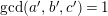 $\gcd (a^{\prime },b^{\prime },c^{\prime })=1$
. Define
$\gcd (a^{\prime },b^{\prime },c^{\prime })=1$
. Define
 $$\begin{eqnarray}\unicode[STIX]{x1D70F}_{1}^{\prime }=\frac{-b^{\prime }+\sqrt{D^{\prime }}}{2a^{\prime }},\qquad \text{and}\qquad \unicode[STIX]{x1D70F}_{2}^{\prime }=\frac{b^{\prime }+\sqrt{D^{\prime }}}{2},\quad \text{where}~D^{\prime }={b^{\prime }}^{2}-4a^{\prime }c^{\prime }.\end{eqnarray}$$
Then, we have
 $\unicode[STIX]{x1D70F}_{1}=\unicode[STIX]{x1D70F}_{1}^{\prime }$
and
$\unicode[STIX]{x1D70F}_{1}=\unicode[STIX]{x1D70F}_{1}^{\prime }$
and
 $\unicode[STIX]{x1D70F}_{2}=m\unicode[STIX]{x1D70F}_{2}^{\prime }$
. Now, suppose that
$\unicode[STIX]{x1D70F}_{2}=m\unicode[STIX]{x1D70F}_{2}^{\prime }$
. Now, suppose that
 $h_{D^{\prime }}=2$
. Then,
$h_{D^{\prime }}=2$
. Then,
 $j(\unicode[STIX]{x1D70F}_{1}^{\prime })$
belongs to some quadratic extension and
$j(\unicode[STIX]{x1D70F}_{1}^{\prime })$
belongs to some quadratic extension and
 $j(\unicode[STIX]{x1D70F}_{2}^{\prime })$
is its conjugate. Since
$j(\unicode[STIX]{x1D70F}_{2}^{\prime })$
is its conjugate. Since
 $j(\unicode[STIX]{x1D70F}_{1}^{\prime })=j(\unicode[STIX]{x1D70F}_{1})$
, in order for our method to work, we need that
$j(\unicode[STIX]{x1D70F}_{1}^{\prime })=j(\unicode[STIX]{x1D70F}_{1})$
, in order for our method to work, we need that
 $j(\unicode[STIX]{x1D70F}_{2})=j(m\unicode[STIX]{x1D70F}_{2}^{\prime })$
is conjugate to
$j(\unicode[STIX]{x1D70F}_{2})=j(m\unicode[STIX]{x1D70F}_{2}^{\prime })$
is conjugate to
 $j(\unicode[STIX]{x1D70F}_{1})$
. But, this implies
$j(\unicode[STIX]{x1D70F}_{1})$
. But, this implies
 $j(\unicode[STIX]{x1D70F}_{2}^{\prime })=j(\unicode[STIX]{x1D70F}_{2})$
and thus the Inose surface corresponding to
$j(\unicode[STIX]{x1D70F}_{2}^{\prime })=j(\unicode[STIX]{x1D70F}_{2})$
and thus the Inose surface corresponding to
 $ax^{2}+bxy+cy^{2}$
and that to
$ax^{2}+bxy+cy^{2}$
and that to
 $a^{\prime }x^{2}+b^{\prime }xy+c^{\prime }y^{2}$
are isomorphic. So, in the nonprimitive case we can reduce to the case of the primitive discriminant
$a^{\prime }x^{2}+b^{\prime }xy+c^{\prime }y^{2}$
are isomorphic. So, in the nonprimitive case we can reduce to the case of the primitive discriminant
 $D$
, corresponding to the latter quadratic form.
$D$
, corresponding to the latter quadratic form.
8.1 Class number 1 case
It is well known that there are thirteen discriminants of class number
 $1$
.
$1$
.
 $$\begin{eqnarray}\displaystyle h_{D} & = & \displaystyle 1\Longleftrightarrow D\nonumber\\ \displaystyle & = & \displaystyle -3,-4,-7,-8,-11,-12,-16,-19,-27,-28,-43,-67,-163.\nonumber\end{eqnarray}$$
(See for example [Reference CoxCo2, Theorem 7.30] and its references.) From these we see that only the fields
 $\mathbb{Q}(\sqrt{-1})$
,
$\mathbb{Q}(\sqrt{-1})$
,
 $\mathbb{Q}(\sqrt{-3})$
and
$\mathbb{Q}(\sqrt{-3})$
and
 $\mathbb{Q}(\sqrt{-7})$
possess nonmaximal order of class number
$\mathbb{Q}(\sqrt{-7})$
possess nonmaximal order of class number
 $1$
. In the following table,
$1$
. In the following table,
 $D$
is a discriminant with
$D$
is a discriminant with
 $h_{D}=1$
,
$h_{D}=1$
,
 $f$
is the conductor of the order,
$f$
is the conductor of the order,
 $\unicode[STIX]{x1D70F}$
is the root of the quadratic form, and
$\unicode[STIX]{x1D70F}$
is the root of the quadratic form, and
 $E$
is an example of
$E$
is an example of
 $E$
having
$E$
having
 $j(\unicode[STIX]{x1D70F})$
as its
$j(\unicode[STIX]{x1D70F})$
as its
 $j$
-invariant.
$j$
-invariant.
Theorem 8.6. Let
 $E_{1}$
and
$E_{1}$
and
 $E_{2}$
be a pair in the table below. Then the Mordell–Weil lattice
$E_{2}$
be a pair in the table below. Then the Mordell–Weil lattice
 $F_{E_{1},E_{2}}^{(n)}(\overline{\mathbb{Q}}(t_{n}))$
for
$F_{E_{1},E_{2}}^{(n)}(\overline{\mathbb{Q}}(t_{n}))$
for
 $n=5,6$
has rank
$n=5,6$
has rank
 $18$
.
$18$
.
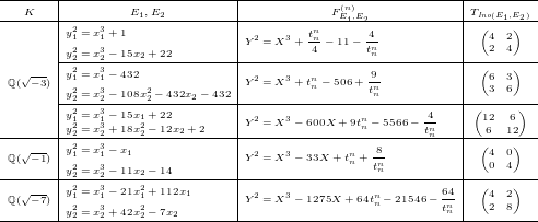
Proof. Elliptic curves belonging to the same
 $K$
in the previous table are isogenous to each other with complex multiplication in some order in
$K$
in the previous table are isogenous to each other with complex multiplication in some order in
 $K$
. They are not isomorphic since
$K$
. They are not isomorphic since
 $j$
-invariants are different. Thus, the Mordell–Weil rank of
$j$
-invariants are different. Thus, the Mordell–Weil rank of
 $F^{(5)}$
and
$F^{(5)}$
and
 $F^{(6)}$
are
$F^{(6)}$
are
 $18$
. Note that the choices of
$18$
. Note that the choices of
 $E_{1}$
and
$E_{1}$
and
 $E_{2}$
are made so that the field of definition of the isogeny is as small as possible.◻
$E_{2}$
are made so that the field of definition of the isogeny is as small as possible.◻
Table 1. Discriminants with class number 2.

Table 2.
 $\mathbb{Q}$
-curves over quadratic fields and associated
$\mathbb{Q}$
-curves over quadratic fields and associated
 $K3$
surfaces.
$K3$
surfaces.
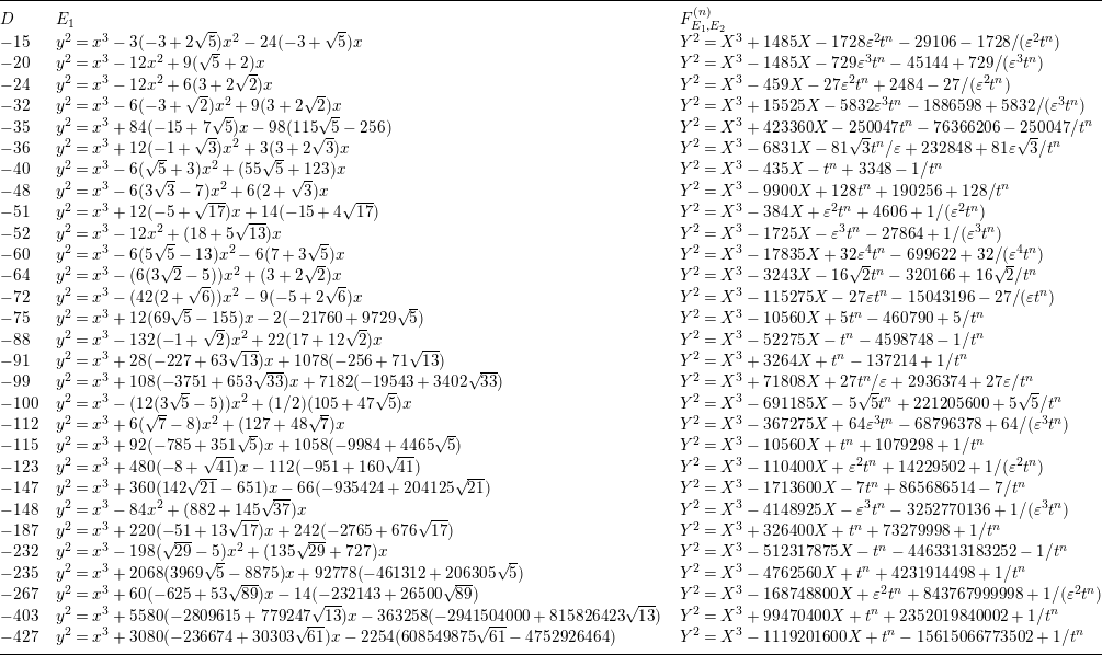
8.2 Class number 2 case
It is also known that there are only finitely many negative discriminants
 $D$
whose class number equals
$D$
whose class number equals
 $2$
(see for example [Reference Ireland and RosenIR, pp. 358–361]). Table 1 shows twenty nine such
$2$
(see for example [Reference Ireland and RosenIR, pp. 358–361]). Table 1 shows twenty nine such
 $D$
, together with
$D$
, together with
 $j(\unicode[STIX]{x1D70F}_{1})$
. Table 2 shows an example of
$j(\unicode[STIX]{x1D70F}_{1})$
. Table 2 shows an example of
 $E_{1}$
for each
$E_{1}$
for each
 $j(\unicode[STIX]{x1D70F}_{1})$
, together with
$j(\unicode[STIX]{x1D70F}_{1})$
, together with
 $F_{E_{1},E_{2}}^{(n)}$
where
$F_{E_{1},E_{2}}^{(n)}$
where
 $E_{2}$
is the Galois conjugate of
$E_{2}$
is the Galois conjugate of
 $E_{1}$
Footnote
3
. In these equations
$E_{1}$
Footnote
3
. In these equations
 $X$
and
$X$
and
 $Y$
are rescaled so that the coefficients become simpler. However,
$Y$
are rescaled so that the coefficients become simpler. However,
 $t$
is the original parameter
$t$
is the original parameter
 $t_{n}$
, and thus some equations contain a variable
$t_{n}$
, and thus some equations contain a variable
 $\unicode[STIX]{x1D700}$
, which indicates the fundamental unit of the real quadratic field
$\unicode[STIX]{x1D700}$
, which indicates the fundamental unit of the real quadratic field
 $\mathbb{Q}(j(\unicode[STIX]{x1D70F}_{1}))$
. By rescaling the elliptic parameter
$\mathbb{Q}(j(\unicode[STIX]{x1D70F}_{1}))$
. By rescaling the elliptic parameter
 $t$
suitably as in Lemma 8.3, we obtain elliptic
$t$
suitably as in Lemma 8.3, we obtain elliptic
 $K3$
surfaces defined over
$K3$
surfaces defined over
 $\mathbb{Q}$
.
$\mathbb{Q}$
.
Theorem 8.7. The twenty-nine Inose surfaces shown in Table 2 are defined over
 $\mathbb{Q}$
and geometrically non-isomorphic. The elliptic fibrations
$\mathbb{Q}$
and geometrically non-isomorphic. The elliptic fibrations
 $F^{(5)}$
and
$F^{(5)}$
and
 $F^{(6)}$
constructed from them have Mordell–Weil rank
$F^{(6)}$
constructed from them have Mordell–Weil rank
 $18$
over
$18$
over
 $\overline{\mathbb{Q}}$
.
$\overline{\mathbb{Q}}$
.
Remark 8.8. As remarked earlier, the equation of the Inose surface may be given in the form
 $$\begin{eqnarray}Y^{2}=X^{3}-3\sqrt[3]{J_{1}J_{2}}\,X+t+\frac{1}{t}-2\sqrt{(1-J_{1})(1-J_{2})},\end{eqnarray}$$
where
 $J_{i}=j(\unicode[STIX]{x1D70F}_{i})/1728$
. Quite often
$J_{i}=j(\unicode[STIX]{x1D70F}_{i})/1728$
. Quite often
 $\sqrt[3]{j(\unicode[STIX]{x1D70F}_{1})j(\unicode[STIX]{x1D70F}_{2})}$
becomes a rational integer (see [Reference CoxCo2, Section 12]), and so does
$\sqrt[3]{j(\unicode[STIX]{x1D70F}_{1})j(\unicode[STIX]{x1D70F}_{2})}$
becomes a rational integer (see [Reference CoxCo2, Section 12]), and so does
 $\sqrt{(1728-j(\unicode[STIX]{x1D70F}_{1}))(1728-j(\unicode[STIX]{x1D70F}_{2}))}$
. In that case the above equation gives a model of the Inose surface over
$\sqrt{(1728-j(\unicode[STIX]{x1D70F}_{1}))(1728-j(\unicode[STIX]{x1D70F}_{2}))}$
. In that case the above equation gives a model of the Inose surface over
 $\mathbb{Q}$
. However, since that is not always the case, we uniformly started from (2.3). By doing so, we can also keep track of the field of definition of
$\mathbb{Q}$
. However, since that is not always the case, we uniformly started from (2.3). By doing so, we can also keep track of the field of definition of
 $F_{E_{1},E_{2}}^{(n)}(\overline{\mathbb{Q}}(t_{n}))$
.
$F_{E_{1},E_{2}}^{(n)}(\overline{\mathbb{Q}}(t_{n}))$
.
9 Examples
In this section, we illustrate the techniques of this paper by working out the Mordell–Weil group explicitly for a few singular K3 surfaces defined over
 $\mathbb{Q}$
. We will use the set-up of the previous section, choosing a few small discriminants. The basic idea is to obtain a finite index sublattice of the Mordell–Weil lattice by combining the formulas in the generic case (when the elliptic curves are non-isogenous) with the extra sections coming from isogenies between the pair of CM curves. To obtain the full Mordell–Weil group, we saturate this sublattice. In practice, this will be most convenient for the surface
$\mathbb{Q}$
. We will use the set-up of the previous section, choosing a few small discriminants. The basic idea is to obtain a finite index sublattice of the Mordell–Weil lattice by combining the formulas in the generic case (when the elliptic curves are non-isogenous) with the extra sections coming from isogenies between the pair of CM curves. To obtain the full Mordell–Weil group, we saturate this sublattice. In practice, this will be most convenient for the surface
 $F^{(6)}$
, for which the Mordell–Weil lattice has sublattices induced from
$F^{(6)}$
, for which the Mordell–Weil lattice has sublattices induced from
 $F^{(3)}$
and its twist, enabling us to proceed in stages. One can also apply our methods to
$F^{(3)}$
and its twist, enabling us to proceed in stages. One can also apply our methods to
 $F^{(5)}$
, which has the disadvantage that saturating the corresponding sublattice is computationally more expensive (but that may be offset by the fact that it is somewhat easier to calculate sections directly, owing to convenient specialization maps at
$F^{(5)}$
, which has the disadvantage that saturating the corresponding sublattice is computationally more expensive (but that may be offset by the fact that it is somewhat easier to calculate sections directly, owing to convenient specialization maps at
 $t=0$
and
$t=0$
and
 $\infty$
). For simplicity we restrict ourselves to
$\infty$
). For simplicity we restrict ourselves to
 $F^{(6)}$
here.
$F^{(6)}$
here.
Example 9.1. (cf. [Reference KuwataKw2, Example 4.5]) Let
 $E_{1}$
and
$E_{1}$
and
 $E_{2}$
be given by
$E_{2}$
be given by
 $$\begin{eqnarray}\displaystyle E_{1}:y_{1}^{2} & = & \displaystyle x_{1}^{3}-x_{1},\nonumber\\ \displaystyle E_{2}:y_{2}^{2} & = & \displaystyle x_{2}^{3}-11x_{2}-14.\nonumber\end{eqnarray}$$
In this case
 $F_{E_{1},E_{2}}^{(n)}$
is given by
$F_{E_{1},E_{2}}^{(n)}$
is given by
 $$\begin{eqnarray}F_{E_{1},E_{2}}^{(n)}:Y^{2}=X^{3}-33X+t_{n}^{n}+\frac{8}{t_{n}^{n}}.\end{eqnarray}$$
The matrix of the quadratic form associated with the Inose surface
 $F_{E_{1},E_{2}}^{(1)}$
is
$F_{E_{1},E_{2}}^{(1)}$
is
 $$\begin{eqnarray}\left(\begin{array}{@{}cc@{}}4 & 0\\ 0 & 4\end{array}\right),\end{eqnarray}$$
so we first identify two
 $2$
-isogenies from
$2$
-isogenies from
 $E_{1}$
to
$E_{1}$
to
 $E_{2}$
. Then using the method described in Section 3.2, we obtain a basis of
$E_{2}$
. Then using the method described in Section 3.2, we obtain a basis of
 $F^{(1)}(\overline{\mathbb{Q}}(t_{1}))$
:
$F^{(1)}(\overline{\mathbb{Q}}(t_{1}))$
:
 $$\begin{eqnarray}\displaystyle P_{1} & = & \displaystyle \left(\frac{1}{144}(s_{1,+}^{2}-72s_{1,+}+400),\frac{1}{1728}s_{1,-}(s_{1,+}^{2}-108s_{1,+}+2560)\right),\nonumber\\ \displaystyle P_{2} & = & \displaystyle \left(-\frac{1}{144}(s_{1,+}^{2}+72s_{1,+}+400),\frac{i}{1728}s_{1,-}(s_{1,+}^{2}+108s_{1,+}+2560)\right),\nonumber\end{eqnarray}$$
where
 $s_{1,+}=t_{1}+8/t_{1}$
and
$s_{1,+}=t_{1}+8/t_{1}$
and
 $s_{1,-}=t_{1}-8/t_{1}$
. Note that we have to extend the base field to
$s_{1,-}=t_{1}-8/t_{1}$
. Note that we have to extend the base field to
 $k=\mathbb{Q}(i)$
to define the isogenies.
$k=\mathbb{Q}(i)$
to define the isogenies.
Next, we study
 $F^{(3)}$
in this example. The images of the above sections in
$F^{(3)}$
in this example. The images of the above sections in
 $F^{(3)}(\overline{\mathbb{Q}}(t_{3}))$
are of height
$F^{(3)}(\overline{\mathbb{Q}}(t_{3}))$
are of height
 $6$
. The splitting field of the
$6$
. The splitting field of the
 $3$
-torsion points of
$3$
-torsion points of
 $E_{1}$
and
$E_{1}$
and
 $E_{2}$
is
$E_{2}$
is
 $$\begin{eqnarray}k(E_{1}[3],E_{2}[3])=\mathbb{Q}(i,\unicode[STIX]{x1D714},12^{1/4}),\quad \text{where}~\unicode[STIX]{x1D714}=(-1+\sqrt{-3})/2.\end{eqnarray}$$
Let
 $\unicode[STIX]{x1D6FC}=\sqrt{3}=-i(2\unicode[STIX]{x1D714}+1)$
,
$\unicode[STIX]{x1D6FC}=\sqrt{3}=-i(2\unicode[STIX]{x1D714}+1)$
,
 $\unicode[STIX]{x1D6FD}=\sqrt{2}$
and
$\unicode[STIX]{x1D6FD}=\sqrt{2}$
and
 $\unicode[STIX]{x1D6FE}=12^{1/4}$
. The sections described in Theorem 4.8 are given by
$\unicode[STIX]{x1D6FE}=12^{1/4}$
. The sections described in Theorem 4.8 are given by
 $$\begin{eqnarray}\displaystyle & \displaystyle P_{3}=\Bigl(-s_{3,+}-9,3i\unicode[STIX]{x1D6FC}(s_{3,+}+4)\Bigr),\qquad P_{4}=\Bigl(-s_{3,+}+9,-3\unicode[STIX]{x1D6FC}(s_{3,+}-4)\Bigr), & \displaystyle \nonumber\\ \displaystyle & \displaystyle P_{5}=\Bigl(-s_{3,+}+i\unicode[STIX]{x1D6FC},\unicode[STIX]{x1D6FE}\unicode[STIX]{x1D6FC}(1+i)/2(-s_{3,+}+2i\unicode[STIX]{x1D6FC})\Bigr), & \displaystyle \nonumber\\ \displaystyle & & \displaystyle \nonumber\end{eqnarray}$$
 $$\begin{eqnarray}\displaystyle P_{6} & = & \displaystyle \Bigl(\unicode[STIX]{x1D714}\big(-s_{3,+}+3\unicode[STIX]{x1D714}(1-i)\unicode[STIX]{x1D6FE}/2+2\unicode[STIX]{x1D6FC}+3i\big),\nonumber\\ \displaystyle & & \displaystyle \quad \big((\unicode[STIX]{x1D714}-1)i\unicode[STIX]{x1D6FE}/2+3(\unicode[STIX]{x1D714}-1)(i+1)/2\big)s_{3,+}+(7i\unicode[STIX]{x1D6FC}-3)\unicode[STIX]{x1D6FE}/2+3(i+1)\unicode[STIX]{x1D6FC}\Bigr),\nonumber\end{eqnarray}$$
 $$\begin{eqnarray}\displaystyle & \displaystyle \unicode[STIX]{x1D70E}^{2}(P_{6}),\qquad \unicode[STIX]{x1D70E}^{2}(P_{5}),\qquad \unicode[STIX]{x1D70E}^{2}(P_{4}),\qquad \unicode[STIX]{x1D70E}^{2}(P_{3}), & \displaystyle \nonumber\end{eqnarray}$$
where
 $s_{3,+}=t_{3}+2/t_{3}$
and
$s_{3,+}=t_{3}+2/t_{3}$
and
 $s_{3,-}=t_{3}-2/t_{3}$
. The height pairing matrix with respect to the above eight sections coincides with the one in Theorem 4.8. Knowing that there are sections of height smaller than
$s_{3,-}=t_{3}-2/t_{3}$
. The height pairing matrix with respect to the above eight sections coincides with the one in Theorem 4.8. Knowing that there are sections of height smaller than
 $6$
independent of the above sections, we search for sections and find the following:
$6$
independent of the above sections, we search for sections and find the following:
 $$\begin{eqnarray}\displaystyle P_{7}=\left(3-s_{3,+},-3s_{3,-}\right)\qquad P_{8}=\left(-3-s_{3,+},-3is_{3,-}\right). & & \displaystyle \nonumber\end{eqnarray}$$
With respect to the basis
 $P_{3},P_{4},P_{5},P_{6},\unicode[STIX]{x1D70E}^{2}(P_{6})\unicode[STIX]{x1D70E}^{2}(P_{5}),\unicode[STIX]{x1D70E}^{2}(P_{4}),\unicode[STIX]{x1D70E}^{2}(P_{3}),P_{7},P_{8}$
the height matrix is
$P_{3},P_{4},P_{5},P_{6},\unicode[STIX]{x1D70E}^{2}(P_{6})\unicode[STIX]{x1D70E}^{2}(P_{5}),\unicode[STIX]{x1D70E}^{2}(P_{4}),\unicode[STIX]{x1D70E}^{2}(P_{3}),P_{7},P_{8}$
the height matrix is
 $$\begin{eqnarray}\left(\begin{array}{@{}rrrrrrrrrr@{}}4 & 0 & 0 & -2 & 1 & 0 & 0 & -2 & 0 & 0\\ 0 & 4 & 0 & -2 & 1 & 0 & -2 & 0 & 0 & 0\\ 0 & 0 & 4 & -2 & 1 & -2 & 0 & 0 & 0 & 0\\ -2 & -2 & -2 & 4 & -2 & 1 & 1 & 1 & 0 & 0\\ 1 & 1 & 1 & -2 & 4 & -2 & -2 & -2 & -1 & -1\\ 0 & 0 & -2 & 1 & -2 & 4 & 0 & 0 & 0 & 0\\ 0 & -2 & 0 & 1 & -2 & 0 & 4 & 0 & 0 & 2\\ -2 & 0 & 0 & 1 & -2 & 0 & 0 & 4 & 2 & 0\\ 0 & 0 & 0 & 0 & -1 & 0 & 0 & 2 & 4 & 0\\ 0 & 0 & 0 & 0 & -1 & 0 & 2 & 0 & 0 & 4\end{array}\right).\end{eqnarray}$$
Note that the Mordell–Weil lattice
 $F^{(3)}(\bar{k}(t_{3}))$
is generated by sections of height
$F^{(3)}(\bar{k}(t_{3}))$
is generated by sections of height
 $4$
in this case.
$4$
in this case.
The rational elliptic surface
 $^{t_{3}}F_{E_{1},E_{2}}^{(3)}$
is
$^{t_{3}}F_{E_{1},E_{2}}^{(3)}$
is
 $$\begin{eqnarray}^{t_{3}}F_{E_{1},E_{2}}^{(3)}:t_{3}Y^{2}=X^{3}-33X+(t_{3}^{3}+8/t_{3}^{3}).\end{eqnarray}$$
In this case
 $\mathbb{Q}(E_{1}[2])=\mathbb{Q}$
and
$\mathbb{Q}(E_{1}[2])=\mathbb{Q}$
and
 $\mathbb{Q}(E_{2}[2])=\mathbb{Q}(\sqrt{2})$
, and
$\mathbb{Q}(E_{2}[2])=\mathbb{Q}(\sqrt{2})$
, and
 $\unicode[STIX]{x1D6E5}_{E_{2}}/\unicode[STIX]{x1D6E5}_{E_{1}}=2^{9}/2^{6}=(\sqrt{2})^{6}$
. So, the field of definition of
$\unicode[STIX]{x1D6E5}_{E_{2}}/\unicode[STIX]{x1D6E5}_{E_{1}}=2^{9}/2^{6}=(\sqrt{2})^{6}$
. So, the field of definition of
 $^{t_{3}}F_{E_{1},E_{2}}^{(3)}(\overline{\mathbb{Q}}(t_{3}))$
is
$^{t_{3}}F_{E_{1},E_{2}}^{(3)}(\overline{\mathbb{Q}}(t_{3}))$
is
 $\mathbb{Q}(\sqrt{2},\unicode[STIX]{x1D714})$
. Following the recipe of Section 7.5, we can obtain a basis of the Mordell–Weil lattice. A small modification of the basis there gives the following simpler basis:
$\mathbb{Q}(\sqrt{2},\unicode[STIX]{x1D714})$
. Following the recipe of Section 7.5, we can obtain a basis of the Mordell–Weil lattice. A small modification of the basis there gives the following simpler basis:
 $$\begin{eqnarray}\displaystyle Q_{1} & = & \displaystyle \big(-\unicode[STIX]{x1D714}^{2}(11t_{3}^{2}+4\unicode[STIX]{x1D714}^{2})/(2t_{3}),-21\unicode[STIX]{x1D6FD}(2\unicode[STIX]{x1D714}+1)t_{3}/4\big)\nonumber\\ \displaystyle Q_{2} & = & \displaystyle \big(2\unicode[STIX]{x1D714}(4-3\unicode[STIX]{x1D6FD})t_{3}-3(1-2\unicode[STIX]{x1D6FD})+4\unicode[STIX]{x1D714}^{2}/t_{3},\nonumber\\ \displaystyle & & \displaystyle \quad 3(11-8\unicode[STIX]{x1D6FD})t_{3}-12\unicode[STIX]{x1D714}^{2}(3-2\unicode[STIX]{x1D6FD})+6\unicode[STIX]{x1D714}(4-\unicode[STIX]{x1D6FD})/t_{3}+6\unicode[STIX]{x1D6FD}/t_{3}^{2}\big)\nonumber\\ \displaystyle Q_{3} & = & \displaystyle \big((2t_{3}^{2}-6t_{3}+1)/t_{3},-3(t_{3}^{3}-4t_{3}^{2}+t_{3}-1)/t_{3}^{2}\big)\nonumber\\ \displaystyle Q_{4} & = & \displaystyle \big(2t_{3}-3(1-2\unicode[STIX]{x1D6FD})+4(4-3\unicode[STIX]{x1D6FD})/t_{3},\nonumber\\ \displaystyle & & \displaystyle \quad -3t_{3}+6(1-2\unicode[STIX]{x1D6FD})-12(4-3\unicode[STIX]{x1D6FD})/t_{3}+(96-66\unicode[STIX]{x1D6FD})/t_{3}^{2}\big)\nonumber\\ \displaystyle Q_{5} & = & \displaystyle \big(-\unicode[STIX]{x1D714}t_{3}+4\unicode[STIX]{x1D714}^{2}(4-3\unicode[STIX]{x1D6FD})/t_{3},-3\unicode[STIX]{x1D714}^{2}(1-2\unicode[STIX]{x1D6FD})+(96-66\unicode[STIX]{x1D6FD})/t_{3}^{2}\big)\nonumber\\ \displaystyle Q_{6} & = & \displaystyle \big(2t_{3}+3(1-2\unicode[STIX]{x1D6FD})+4(4-3\unicode[STIX]{x1D6FD})/t_{3},\nonumber\\ \displaystyle & & \displaystyle \quad 3t_{3}+6(1-2\unicode[STIX]{x1D6FD})+12(4-3\unicode[STIX]{x1D6FD})/t_{3}+(96-66\unicode[STIX]{x1D6FD})/t_{3}^{2}\big)\nonumber\\ \displaystyle Q_{7} & = & \displaystyle \big((2t_{3}^{2}+6t_{3}+1)/t_{3},3(t_{3}^{3}+4t_{3}^{2}+t_{3}+1)/t_{3}^{2}\big)\nonumber\\ \displaystyle Q_{8} & = & \displaystyle \big(-t_{3}-11/t_{3},21(1+2\unicode[STIX]{x1D714})/t_{3}^{2}\big)\nonumber\end{eqnarray}$$
which gives the height pairing matrix
 $$\begin{eqnarray}\left(\begin{array}{@{}rrrrrrrr@{}}2 & -1 & 0 & 0 & 0 & 0 & 0 & 0\\ -1 & 2 & -1 & 0 & 0 & 0 & 0 & 0\\ 0 & -1 & 2 & -1 & 0 & 0 & 0 & 0\\ 0 & 0 & -1 & 2 & -1 & 0 & 0 & 0\\ 0 & 0 & 0 & -1 & 2 & -1 & 0 & -1\\ 0 & 0 & 0 & 0 & -1 & 2 & -1 & 0\\ 0 & 0 & 0 & 0 & 0 & -1 & 2 & 0\\ 0 & 0 & 0 & 0 & -1 & 0 & 0 & 2\end{array}\right).\end{eqnarray}$$
In order to find a basis for
 $$\begin{eqnarray}F_{E_{1},E_{2}}^{(6)}:Y^{2}=X^{3}-33t_{6}^{4}X+(t_{6}^{12}+8),\end{eqnarray}$$
we have to fill the gap between
 $L^{\prime }=F_{E_{1},E_{2}}^{(3)}(\bar{k}(t_{3}))\oplus ^{t_{3}}F_{E_{1},E_{2}}^{(3)}(\bar{k}(t_{3}))$
and
$L^{\prime }=F_{E_{1},E_{2}}^{(3)}(\bar{k}(t_{3}))\oplus ^{t_{3}}F_{E_{1},E_{2}}^{(3)}(\bar{k}(t_{3}))$
and
 $L=F_{E_{1},E_{2}}^{(6)}(\bar{k}(t_{6}))$
. The lattices differ by a power-of-two index. In principle, this is a routine calculation; we simply have to check whether nontrivial coset of
$L=F_{E_{1},E_{2}}^{(6)}(\bar{k}(t_{6}))$
. The lattices differ by a power-of-two index. In principle, this is a routine calculation; we simply have to check whether nontrivial coset of
 $L^{\prime }$
modulo
$L^{\prime }$
modulo
 $2L^{\prime }$
is twice an element of the Mordell–Weil group
$2L^{\prime }$
is twice an element of the Mordell–Weil group
 $L$
, and this boils down to checking whether a suitable equation has a root in
$L$
, and this boils down to checking whether a suitable equation has a root in
 $\bar{k}(t_{6})$
. However, there are
$\bar{k}(t_{6})$
. However, there are
 $2^{18}-1$
such cosets, and the number field involved is quite large, so we need to speed up the process by reducing the large number of possible candidate cosets.
$2^{18}-1$
such cosets, and the number field involved is quite large, so we need to speed up the process by reducing the large number of possible candidate cosets.
To do so, we apply the following useful procedure (a similar trick was used in [Reference ShiodaSh6]). First reduce modulo a suitable prime
 $p$
such that all the 6-torsion points are defined over
$p$
such that all the 6-torsion points are defined over
 $\mathbb{F}_{p}$
. In our case
$\mathbb{F}_{p}$
. In our case
 $p=193$
will do, as
$p=193$
will do, as
 $x^{4}+1$
and
$x^{4}+1$
and
 $x^{4}-3$
split into linear factors. Since arithmetic modulo
$x^{4}-3$
split into linear factors. Since arithmetic modulo
 $p$
is cheap, we can do the search mentioned in the previous paragraph fairly quickly. This pins down the likely candidates, and now we may solve the equation back in the original number field
$p$
is cheap, we can do the search mentioned in the previous paragraph fairly quickly. This pins down the likely candidates, and now we may solve the equation back in the original number field
 $k$
for each of them. We find new sections
$k$
for each of them. We find new sections
 $R_{1},\ldots ,R_{5}$
which satisfy the relations
$R_{1},\ldots ,R_{5}$
which satisfy the relations
 $$\begin{eqnarray}\displaystyle 2R_{1} & = & \displaystyle P_{3}-P_{7}-Q_{3}-2Q_{4}-2Q_{5}-Q_{8}\nonumber\\ \displaystyle 2R_{2} & = & \displaystyle -P_{3}-P_{5}-2P_{6}-\unicode[STIX]{x1D70E}^{2}(P_{3})+\unicode[STIX]{x1D70E}^{2}(P_{4})+P_{7}-P_{8}\nonumber\\ \displaystyle & & \displaystyle +\,Q_{3}+2Q_{4}+2Q_{5}+2Q_{6}+Q_{7}+Q_{8}\nonumber\\ \displaystyle 2R_{3} & = & \displaystyle -P_{4}-P_{5}-\unicode[STIX]{x1D70E}^{2}(P_{4})-\unicode[STIX]{x1D70E}^{2}(P_{5})-P_{7}+P_{8}+Q_{3}+Q_{4}+Q_{5}+Q_{6}+Q_{7}\nonumber\\ \displaystyle 2R_{4} & = & \displaystyle P_{3}-P_{4}-Q_{1}-Q_{2}-2Q_{3}-3Q_{4}-4Q_{5}-4Q_{6}-2Q_{7}-2Q_{8}\nonumber\\ \displaystyle 2R_{5} & = & \displaystyle \unicode[STIX]{x1D70E}^{2}(P_{3})-\unicode[STIX]{x1D70E}^{2}(P_{4})+Q_{1}+2Q_{2}+2Q_{3}+3Q_{4}+3Q_{5}+Q_{6}+Q_{8}.\nonumber\end{eqnarray}$$
Recall that
 $\unicode[STIX]{x1D70E}=\unicode[STIX]{x1D70E}_{6}$
is the map
$\unicode[STIX]{x1D70E}=\unicode[STIX]{x1D70E}_{6}$
is the map
 $\big(X(t_{6}),Y(t_{6})\big)\mapsto \big(X(t_{6}/\unicode[STIX]{x1D701}_{6}),Y(t_{6}/\unicode[STIX]{x1D701}_{6})\big)$
. The expressions for the
$\big(X(t_{6}),Y(t_{6})\big)\mapsto \big(X(t_{6}/\unicode[STIX]{x1D701}_{6}),Y(t_{6}/\unicode[STIX]{x1D701}_{6})\big)$
. The expressions for the
 $x$
- and
$x$
- and
 $y$
-coordinates of these new sections may be found in the auxiliary files; apart from
$y$
-coordinates of these new sections may be found in the auxiliary files; apart from
 $R_{1}$
, which is shown below, they are quite complicated.
$R_{1}$
, which is shown below, they are quite complicated.
 $$\begin{eqnarray}\displaystyle R_{1} & = & \displaystyle (-\unicode[STIX]{x1D714}t_{6}^{2}+3+6\unicode[STIX]{x1D714}\unicode[STIX]{x1D6FD}/t_{6}+4\unicode[STIX]{x1D714}^{2}/t_{6}^{2},\nonumber\\ \displaystyle & & \displaystyle \quad -3\unicode[STIX]{x1D714}t_{6}^{2}-3\unicode[STIX]{x1D714}^{2}\unicode[STIX]{x1D6FD}t_{6}+18\unicode[STIX]{x1D714}\unicode[STIX]{x1D6FD}/t_{6}+24\unicode[STIX]{x1D714}^{2}/t_{6}^{2}+6\unicode[STIX]{x1D6FD}/t_{6}^{3}).\nonumber\end{eqnarray}$$
The sections
 $$\begin{eqnarray}\displaystyle & & \displaystyle P_{4},P_{5},P_{6},\unicode[STIX]{x1D70E}^{2}(P_{6}),\unicode[STIX]{x1D70E}^{2}(P_{5}),P_{7},P_{8},Q_{1},Q_{3},Q_{4},Q_{6},Q_{7},R_{1},\nonumber\\ \displaystyle & & \displaystyle \quad R_{2},\unicode[STIX]{x1D70E}^{-1}(R_{2}),R_{3},R_{4},R_{5},\nonumber\end{eqnarray}$$
form a basis of the Mordell–Weil lattice
 $F^{(6)}(\overline{\mathbb{Q}}(t_{6}))$
. The height pairing matrix with respect to this basis is
$F^{(6)}(\overline{\mathbb{Q}}(t_{6}))$
. The height pairing matrix with respect to this basis is
 $$\begin{eqnarray}\left(\begin{array}{@{}rrrrrrrrrrrrrrrrrr@{}}4 & 0 & -2 & 1 & 0 & 0 & 0 & 0 & 0 & 0 & 0 & 0 & 0 & 1 & -1 & -1 & -2 & 1\\ 0 & 4 & -2 & 1 & -2 & 0 & 0 & 0 & 0 & 0 & 0 & 0 & 0 & 0 & 0 & -1 & 0 & 0\\ -2 & -2 & 4 & -2 & 1 & 0 & 0 & 0 & 0 & 0 & 0 & 0 & -1 & -2 & 1 & 1 & 0 & 0\\ 1 & 1 & -2 & 4 & -2 & -1 & -1 & 0 & 0 & 0 & 0 & 0 & 1 & 1 & -2 & 1 & 0 & 0\\ 0 & -2 & 1 & -2 & 4 & 0 & 0 & 0 & 0 & 0 & 0 & 0 & 0 & 0 & 0 & -1 & 0 & 0\\ 0 & 0 & 0 & -1 & 0 & 4 & 0 & 0 & 0 & 0 & 0 & 0 & -2 & 1 & 2 & -2 & 0 & 1\\ 0 & 0 & 0 & -1 & 0 & 0 & 4 & 0 & 0 & 0 & 0 & 0 & 0 & -1 & -1 & 1 & 0 & -1\\ 0 & 0 & 0 & 0 & 0 & 0 & 0 & 4 & 0 & 0 & 0 & 0 & 0 & 0 & 0 & 0 & -1 & 0\\ 0 & 0 & 0 & 0 & 0 & 0 & 0 & 0 & 4 & -2 & 0 & 0 & 0 & 0 & -1 & 1 & 0 & -1\\ 0 & 0 & 0 & 0 & 0 & 0 & 0 & 0 & -2 & 4 & 0 & 0 & -1 & 1 & 0 & 0 & 0 & 1\\ 0 & 0 & 0 & 0 & 0 & 0 & 0 & 0 & 0 & 0 & 4 & -2 & 2 & 1 & 0 & 0 & -2 & -1\\ 0 & 0 & 0 & 0 & 0 & 0 & 0 & 0 & 0 & 0 & -2 & 4 & 0 & 0 & -1 & 1 & 0 & -1\\ 0 & 0 & -1 & 1 & 0 & -2 & 0 & 0 & 0 & -1 & 2 & 0 & 4 & 0 & -1 & 1 & 0 & -2\\ 1 & 0 & -2 & 1 & 0 & 1 & -1 & 0 & 0 & 1 & 1 & 0 & 0 & 4 & 0 & -1 & -1 & -1\\ -1 & 0 & 1 & -2 & 0 & 2 & -1 & 0 & -1 & 0 & 0 & -1 & -1 & 0 & 4 & -2 & 1 & 1\\ -1 & -1 & 1 & 1 & -1 & -2 & 1 & 0 & 1 & 0 & 0 & 1 & 1 & -1 & -2 & 4 & 0 & -1\\ -2 & 0 & 0 & 0 & 0 & 0 & 0 & -1 & 0 & 0 & -2 & 0 & 0 & -1 & 1 & 0 & 4 & 0\\ 1 & 0 & 0 & 0 & 0 & 1 & -1 & 0 & -1 & 1 & -1 & -1 & -2 & -1 & 1 & -1 & 0 & 4\end{array}\right).\end{eqnarray}$$
Its determinant equals
 $576=2^{6}3^{2}$
, as expected. Note that this Mordell–Weil lattice is generated by sections of height
$576=2^{6}3^{2}$
, as expected. Note that this Mordell–Weil lattice is generated by sections of height
 $4$
. The field of definition for the Mordell–Weil lattice of
$4$
. The field of definition for the Mordell–Weil lattice of
 $F^{(6)}$
is
$F^{(6)}$
is
 $\mathbb{Q}(i,\unicode[STIX]{x1D714},12^{1/4},\sqrt{2})=\mathbb{Q}(\sqrt{-1},\sqrt{2},3^{1/4})$
.
$\mathbb{Q}(i,\unicode[STIX]{x1D714},12^{1/4},\sqrt{2})=\mathbb{Q}(\sqrt{-1},\sqrt{2},3^{1/4})$
.
Example 9.2. Let
 $E_{1}$
and
$E_{1}$
and
 $E_{2}$
be given by
$E_{2}$
be given by
 $$\begin{eqnarray}\displaystyle E_{1}:y_{1}^{2} & = & \displaystyle x_{1}^{3}-21x_{1}^{2}+112x_{1},\nonumber\\ \displaystyle E_{2}:y_{2}^{2} & = & \displaystyle x_{2}^{3}+42x_{2}^{2}-7x_{2}.\nonumber\end{eqnarray}$$
They have complex multiplication by
 $\unicode[STIX]{x1D6FC}=\sqrt{-7}$
. The matrix of the quadratic form associated with the Inose surface
$\unicode[STIX]{x1D6FC}=\sqrt{-7}$
. The matrix of the quadratic form associated with the Inose surface
 $F_{E_{1},E_{2}}^{(1)}$
is
$F_{E_{1},E_{2}}^{(1)}$
is
 $$\begin{eqnarray}\left(\begin{array}{@{}cc@{}}4 & 2\\ 2 & 8\end{array}\right),\end{eqnarray}$$
so there are
 $2$
- and
$2$
- and
 $4$
-isogenies from
$4$
-isogenies from
 $E_{1}$
to
$E_{1}$
to
 $E_{2}$
. The
$E_{2}$
. The
 $2$
-isogeny
$2$
-isogeny
 $\unicode[STIX]{x1D711}:E_{1}\rightarrow E_{2}$
is given by
$\unicode[STIX]{x1D711}:E_{1}\rightarrow E_{2}$
is given by
 $$\begin{eqnarray}\unicode[STIX]{x1D711}(x_{1},y_{1})=\left(\frac{x_{1}^{2}-21x_{1}+112}{x_{1}},\frac{y_{1}(x_{1}^{2}-112)}{x_{1}^{2}}\right).\end{eqnarray}$$
Also, there is a
 $4$
-isogeny
$4$
-isogeny
 $\unicode[STIX]{x1D713}:E_{1}\rightarrow E_{2}$
given by
$\unicode[STIX]{x1D713}:E_{1}\rightarrow E_{2}$
given by
 $\unicode[STIX]{x1D713}(x_{1},y_{1})=(x_{2},y_{2})$
, where the
$\unicode[STIX]{x1D713}(x_{1},y_{1})=(x_{2},y_{2})$
, where the
 $x$
-coordinate is given by
$x$
-coordinate is given by
 $$\begin{eqnarray}\displaystyle x_{2}=\frac{-(3+\unicode[STIX]{x1D6FC})x_{1}(2x_{1}-21-\unicode[STIX]{x1D6FC})(x_{1}-7-\unicode[STIX]{x1D6FC})^{2}}{8(x_{1}-14+2\unicode[STIX]{x1D6FC})^{2}(2x_{1}-21+\unicode[STIX]{x1D6FC})}. & & \displaystyle \nonumber\end{eqnarray}$$
For the
 $2$
-isogeny
$2$
-isogeny
 $\unicode[STIX]{x1D711}$
, the intersection (3.2) consists of the image of
$\unicode[STIX]{x1D711}$
, the intersection (3.2) consists of the image of
 $2$
-torsion points and two effective divisors
$2$
-torsion points and two effective divisors
 $D^{\pm }$
of degree
$D^{\pm }$
of degree
 $2$
defined over
$2$
defined over
 $\mathbb{Q}(t_{2})$
. Write
$\mathbb{Q}(t_{2})$
. Write
 $D_{\unicode[STIX]{x1D711}}^{\pm }=P_{1}^{\pm }+P_{2}^{\pm }$
, where
$D_{\unicode[STIX]{x1D711}}^{\pm }=P_{1}^{\pm }+P_{2}^{\pm }$
, where
 $P_{1}^{\pm }$
and
$P_{1}^{\pm }$
and
 $P_{2}^{\pm }$
are points on the cubic curve defined over
$P_{2}^{\pm }$
are points on the cubic curve defined over
 $\overline{\mathbb{Q}}(t_{2})$
. Let
$\overline{\mathbb{Q}}(t_{2})$
. Let
 $L^{\pm }$
be the line passing through
$L^{\pm }$
be the line passing through
 $P_{1}^{\pm }$
and
$P_{1}^{\pm }$
and
 $P_{2}^{\pm }$
. Then, each third point of intersection
$P_{2}^{\pm }$
. Then, each third point of intersection
 $P_{3}^{\pm }$
is a
$P_{3}^{\pm }$
is a
 $\mathbb{Q}(t_{2})$
rational point, given by
$\mathbb{Q}(t_{2})$
rational point, given by
 $$\begin{eqnarray}(x_{1}^{\pm },x_{2}^{\pm })=\left(\frac{84}{t_{2}^{2}\pm 4t_{2}+8},-\frac{21t_{2}^{2}}{t_{2}^{2}\pm 4t_{2}+8}\right).\end{eqnarray}$$
For the
 $4$
-isogeny
$4$
-isogeny
 $\unicode[STIX]{x1D713}$
, the intersection (3.2) consists of the image of
$\unicode[STIX]{x1D713}$
, the intersection (3.2) consists of the image of
 $2$
-torsion points and two effective divisors
$2$
-torsion points and two effective divisors
 $D_{\unicode[STIX]{x1D713}}^{\pm }$
of degree
$D_{\unicode[STIX]{x1D713}}^{\pm }$
of degree
 $5$
defined over
$5$
defined over
 $\mathbb{Q}(\sqrt{-7})(t_{2})$
. Write
$\mathbb{Q}(\sqrt{-7})(t_{2})$
. Write
 $D_{\unicode[STIX]{x1D713}}^{\pm }=Q_{1}^{\pm }+\cdots +Q_{5}^{\pm }$
, where
$D_{\unicode[STIX]{x1D713}}^{\pm }=Q_{1}^{\pm }+\cdots +Q_{5}^{\pm }$
, where
 $Q_{1}^{\pm },\ldots ,Q_{5}^{\pm }$
are points on the cubic curve defined over
$Q_{1}^{\pm },\ldots ,Q_{5}^{\pm }$
are points on the cubic curve defined over
 $\overline{\mathbb{Q}}(t_{2})$
. There exists conics
$\overline{\mathbb{Q}}(t_{2})$
. There exists conics
 $C^{\pm }$
passing through these five points
$C^{\pm }$
passing through these five points
 $Q_{1}^{\pm },\ldots ,Q_{5}^{\pm }$
. Then, the sixth point of intersection
$Q_{1}^{\pm },\ldots ,Q_{5}^{\pm }$
. Then, the sixth point of intersection
 $Q_{6}^{\pm }$
of
$Q_{6}^{\pm }$
of
 $C^{\pm }$
with the cubic curve is a
$C^{\pm }$
with the cubic curve is a
 $\mathbb{Q}(\sqrt{-7})(t_{2})$
-rational point. The problem of finding the coordinates
$\mathbb{Q}(\sqrt{-7})(t_{2})$
-rational point. The problem of finding the coordinates
 $(x_{1}^{\pm },x_{2}^{\pm })$
of
$(x_{1}^{\pm },x_{2}^{\pm })$
of
 $Q_{6}^{\pm }$
can be reduced to a linear algebra problem of determining the coefficients of
$Q_{6}^{\pm }$
can be reduced to a linear algebra problem of determining the coefficients of
 $C^{\pm }$
. Namely, let
$C^{\pm }$
. Namely, let
 $p(x_{1})$
be the quintic equation satisfied by the
$p(x_{1})$
be the quintic equation satisfied by the
 $x_{1}$
-coordinates of the five points
$x_{1}$
-coordinates of the five points
 $Q_{i}^{\pm }$
, with coefficients in
$Q_{i}^{\pm }$
, with coefficients in
 $K=\mathbb{Q}(\sqrt{-7})(t_{2})$
. We work in the field
$K=\mathbb{Q}(\sqrt{-7})(t_{2})$
. We work in the field
 $L=K[x_{1}]/(p(x_{1}))$
. Then, we compute
$L=K[x_{1}]/(p(x_{1}))$
. Then, we compute
 $x_{2}$
in terms of
$x_{2}$
in terms of
 $x_{1}$
, which follows from the quartic equation
$x_{1}$
, which follows from the quartic equation
 $\unicode[STIX]{x1D713}_{y}(x_{1})=\pm t_{2}$
, and it is an element of
$\unicode[STIX]{x1D713}_{y}(x_{1})=\pm t_{2}$
, and it is an element of
 $L$
. So, now if we make the
$L$
. So, now if we make the
 $5$
by
$5$
by
 $6$
matrix whose columns are the coordinates of
$6$
matrix whose columns are the coordinates of
 $1,x_{1},x_{2},x_{1}x_{2},x_{1}^{2},x_{2}^{2}$
in terms of the basis
$1,x_{1},x_{2},x_{1}x_{2},x_{1}^{2},x_{2}^{2}$
in terms of the basis
 $(1,x_{1},x_{1}^{2},x_{1}^{3},x_{1}^{4})$
of
$(1,x_{1},x_{1}^{2},x_{1}^{3},x_{1}^{4})$
of
 $L$
as a
$L$
as a
 $K$
-vector space, we just need to take the kernel of this matrix (which has coefficients in
$K$
-vector space, we just need to take the kernel of this matrix (which has coefficients in
 $K$
). The
$K$
). The
 $1$
-dimensional kernel gives us the coefficients of the conic. From there, by taking resultants and factoring, we obtain the sixth point. It is given by
$1$
-dimensional kernel gives us the coefficients of the conic. From there, by taking resultants and factoring, we obtain the sixth point. It is given by
 $(x_{1}^{\pm },x_{2}^{\pm })=(x_{1,n}^{\pm }/d^{\pm },x_{2,n}^{\pm }/d^{\pm })$
, where
$(x_{1}^{\pm },x_{2}^{\pm })=(x_{1,n}^{\pm }/d^{\pm },x_{2,n}^{\pm }/d^{\pm })$
, where
 $$\begin{eqnarray}\displaystyle x_{1,n}^{\pm } & = & \displaystyle (\pm 2t+5+\unicode[STIX]{x1D6FC})((21-\unicode[STIX]{x1D6FC})t^{4}\pm 2(91-15\unicode[STIX]{x1D6FC})t^{3}\nonumber\\ \displaystyle & & \displaystyle \quad +\,2(259-11\unicode[STIX]{x1D6FC})t^{2}\pm 2(63+29\unicode[STIX]{x1D6FC})t-7+3\unicode[STIX]{x1D6FC}),\nonumber\\ \displaystyle x_{2,n}^{\pm } & = & \displaystyle -3(\pm 7t-\unicode[STIX]{x1D6FC})(\pm 2t-5-\unicode[STIX]{x1D6FC})(\pm 2t+5+\unicode[STIX]{x1D6FC})t^{2},\nonumber\\ \displaystyle d^{\pm } & = & \displaystyle 2(\pm 2t^{5}+(23-\unicode[STIX]{x1D6FC})t^{4}\pm (117-19\unicode[STIX]{x1D6FC})t^{3}\nonumber\\ \displaystyle & & \displaystyle \quad +\,(109+29\unicode[STIX]{x1D6FC})t^{2}\mp 2(1-9\unicode[STIX]{x1D6FC})t-5+\unicode[STIX]{x1D6FC}).\nonumber\end{eqnarray}$$
Over
 $\mathbb{Q}(\sqrt{-7})$
, the Weierstrass equation of the elliptic curve
$\mathbb{Q}(\sqrt{-7})$
, the Weierstrass equation of the elliptic curve
 $F_{E_{1},E_{2}}^{(n)}$
is given by
$F_{E_{1},E_{2}}^{(n)}$
is given by
 $$\begin{eqnarray}F_{E_{1},E_{2}}^{(n)}:Y^{2}=X^{3}-1275X+64\,t_{n}^{n}-21546-\frac{64}{t_{n}^{n}}.\end{eqnarray}$$
Using the construction of Proposition 3.2, the points obtained above yield points in
 $F^{(1)}(\bar{k}(t_{1}))$
 $$\begin{eqnarray}\displaystyle (X,Y) & = & \displaystyle \left(-\frac{1}{63}\Bigl(4s_{1,-}^{2}-252s_{1,-}+1339\Bigr),\right.\nonumber\\ \displaystyle & & \displaystyle \quad \left.\frac{4}{1323}\unicode[STIX]{x1D6FC}s_{1,+}\Bigl(2s_{1,-}^{2}-189s_{1,-}+3977\Bigr)\right),\nonumber\end{eqnarray}$$
and
 $(X,Y)=(X_{0}/d^{2},Y_{0}/d^{3})$
, where
$(X,Y)=(X_{0}/d^{2},Y_{0}/d^{3})$
, where
 $$\begin{eqnarray}\displaystyle X_{0} & = & \displaystyle \Bigl(\frac{1-\unicode[STIX]{x1D6FC}}{2}\Bigr)^{4}s_{1,-}^{4}+16(33-4\unicode[STIX]{x1D6FC})\Bigl(\frac{1+\unicode[STIX]{x1D6FC}}{2}\Bigr)^{4}s_{1,-}^{3}+36(1783+324\unicode[STIX]{x1D6FC})s_{1,-}^{2}\nonumber\\ \displaystyle & & \displaystyle +\,16(100923+3701\unicode[STIX]{x1D6FC})\Bigl(\frac{1+\unicode[STIX]{x1D6FC}}{2}\Bigr)^{4}s_{1,-}+64(12531+3413\unicode[STIX]{x1D6FC})\Bigl(\frac{1+\unicode[STIX]{x1D6FC}}{2}\Bigr)^{6},\nonumber\\ \displaystyle Y_{0} & = & \displaystyle s_{1,+}\Bigl(-\Bigl(\frac{1-\unicode[STIX]{x1D6FC}}{2}\Bigr)^{6}s_{1,-}^{5}-96(33-4\unicode[STIX]{x1D6FC})\Bigl(\frac{1+\unicode[STIX]{x1D6FC}}{2}\Bigr)^{2}s_{1,-}^{4}\nonumber\\ \displaystyle & & \displaystyle +\,2^{5}(2531+1260\unicode[STIX]{x1D6FC})\Bigl(\frac{1+\unicode[STIX]{x1D6FC}}{2}\Bigr)^{6}s_{1,-}^{3}-2^{7}(18898-98053\unicode[STIX]{x1D6FC})\Bigl(\frac{1+\unicode[STIX]{x1D6FC}}{2}\Bigr)s_{1,-}^{2}\nonumber\\ \displaystyle & & \displaystyle -\,2^{10}(1735197-165636\unicode[STIX]{x1D6FC})\Bigl(\frac{1+\unicode[STIX]{x1D6FC}}{2}\Bigr)^{2}s_{1,-}\nonumber\\ \displaystyle & & \displaystyle -\,2^{14}(58959-85160\unicode[STIX]{x1D6FC})\Bigl(\frac{1+\unicode[STIX]{x1D6FC}}{2}\Bigr)^{6}\Bigr)\nonumber\\ \displaystyle d & = & \displaystyle 6((11+4\unicode[STIX]{x1D6FC})s_{1,-}-4(1-11\unicode[STIX]{x1D6FC})).\nonumber\end{eqnarray}$$
Here we have used
 $s_{1,+}=t_{1}+1/t_{1}$
and
$s_{1,+}=t_{1}+1/t_{1}$
and
 $s_{1,-}=t_{1}-1/t_{1}$
to condense the above formulas. These points form a basis of
$s_{1,-}=t_{1}-1/t_{1}$
to condense the above formulas. These points form a basis of
 $F^{(1)}(\bar{k}(t_{1}))$
, and the height matrix is given by
$F^{(1)}(\bar{k}(t_{1}))$
, and the height matrix is given by
 $$\begin{eqnarray}\left(\begin{array}{@{}cc@{}}2 & -1\\ -1 & 4\end{array}\right).\end{eqnarray}$$
One can proceed to compute the Mordell–Weil group of
 $F^{(6)}$
; this is done in the auxiliary files. The field of definition is
$F^{(6)}$
; this is done in the auxiliary files. The field of definition is
 $\mathbb{Q}\Big(\sqrt{-1},\sqrt{3},\sqrt{(3+\sqrt{21})/2}\Big)$
.
$\mathbb{Q}\Big(\sqrt{-1},\sqrt{3},\sqrt{(3+\sqrt{21})/2}\Big)$
.
Example 9.3. Discriminant
 $\unicode[STIX]{x1D6E5}=-15$
.
$\unicode[STIX]{x1D6E5}=-15$
.
The class number of
 $\unicode[STIX]{x1D6E5}=-15$
is
$\unicode[STIX]{x1D6E5}=-15$
is
 $2$
, and the nontrivial quadratic form is represented by
$2$
, and the nontrivial quadratic form is represented by
 $$\begin{eqnarray}\left(\begin{array}{@{}cc@{}}4 & 1\\ 1 & 4\end{array}\right)\qquad \text{or}\qquad 2x^{2}+xy+2y^{2}.\end{eqnarray}$$
The Hilbert class field of
 $K=\mathbb{Q}(\sqrt{-15})$
equals
$K=\mathbb{Q}(\sqrt{-15})$
equals
 $H=K(\sqrt{5})$
. The value of
$H=K(\sqrt{5})$
. The value of
 $j(\unicode[STIX]{x1D70F})$
for
$j(\unicode[STIX]{x1D70F})$
for
 $\unicode[STIX]{x1D70F}_{1}=(-1+\sqrt{-15})/4$
and
$\unicode[STIX]{x1D70F}_{1}=(-1+\sqrt{-15})/4$
and
 $\unicode[STIX]{x1D70F}_{2}=(1+\sqrt{-15})/2$
are given by
$\unicode[STIX]{x1D70F}_{2}=(1+\sqrt{-15})/2$
are given by
 $$\begin{eqnarray}\displaystyle j(\unicode[STIX]{x1D70F}_{1}) & = & \displaystyle \frac{-191025+85995\sqrt{5}}{2}=\bar{\unicode[STIX]{x1D702}}^{5}(3\unicode[STIX]{x1D70B}_{5}\bar{\unicode[STIX]{x1D70B}}_{11})^{3},\nonumber\\ \displaystyle j(\unicode[STIX]{x1D70F}_{2}) & = & \displaystyle \frac{-191025-85995\sqrt{5}}{2}=-\unicode[STIX]{x1D702}^{5}(3\unicode[STIX]{x1D70B}_{5}\unicode[STIX]{x1D70B}_{11})^{3},\nonumber\end{eqnarray}$$
where
 $\unicode[STIX]{x1D702}=(1+\sqrt{5})/2$
(the Golden ratio) is the fundamental unit of
$\unicode[STIX]{x1D702}=(1+\sqrt{5})/2$
(the Golden ratio) is the fundamental unit of
 $\mathbb{Q}(\sqrt{5})$
,
$\mathbb{Q}(\sqrt{5})$
,
 $\unicode[STIX]{x1D70B}_{5}=\sqrt{5}$
,
$\unicode[STIX]{x1D70B}_{5}=\sqrt{5}$
,
 $\unicode[STIX]{x1D70B}_{11}=(1+3\sqrt{5})/2$
is the generator of a prime ideal above
$\unicode[STIX]{x1D70B}_{11}=(1+3\sqrt{5})/2$
is the generator of a prime ideal above
 $11$
, and
$11$
, and
 $\bar{\quad }$
indicates the conjugate
$\bar{\quad }$
indicates the conjugate
 $\sqrt{5}\mapsto -\sqrt{5}$
. We also have
$\sqrt{5}\mapsto -\sqrt{5}$
. We also have
 $$\begin{eqnarray}\displaystyle j(\unicode[STIX]{x1D70F}_{1})-1728 & = & \displaystyle -3^{3}(\bar{\unicode[STIX]{x1D702}}^{3}7\unicode[STIX]{x1D70B}_{11})^{2},\nonumber\\ \displaystyle j(\unicode[STIX]{x1D70F}_{2})-1728 & = & \displaystyle -3^{3}(\unicode[STIX]{x1D702}^{3}7\bar{\unicode[STIX]{x1D70B}}_{11})^{2}.\nonumber\end{eqnarray}$$
We remark that in this case
 $j(\unicode[STIX]{x1D70F}_{i})$
are not perfect cubes in
$j(\unicode[STIX]{x1D70F}_{i})$
are not perfect cubes in
 $H$
. Although the
$H$
. Although the
 $j(\unicode[STIX]{x1D70F}_{i})-1728$
are not perfect squares over
$j(\unicode[STIX]{x1D70F}_{i})-1728$
are not perfect squares over
 $K$
, they are perfect squares in
$K$
, they are perfect squares in
 $H$
as
$H$
as
 $H$
contains
$H$
contains
 $\sqrt{-3}=\sqrt{-15}/\sqrt{5}$
.
$\sqrt{-3}=\sqrt{-15}/\sqrt{5}$
.
One of the elliptic curves whose
 $j$
-invariant equals
$j$
-invariant equals
 $j(\unicode[STIX]{x1D70F}_{1})$
and
$j(\unicode[STIX]{x1D70F}_{1})$
and
 $j(\unicode[STIX]{x1D70F}_{2})$
are
$j(\unicode[STIX]{x1D70F}_{2})$
are
 $$\begin{eqnarray}\displaystyle E_{1}:y^{2} & = & \displaystyle x^{3}-3(3-2\sqrt{5})x^{2}+24(3-\sqrt{5})x,\nonumber\\ \displaystyle E_{2}:y^{2} & = & \displaystyle x^{3}-3(3+2\sqrt{5})x^{2}+24(3+\sqrt{5})x.\nonumber\end{eqnarray}$$
There are two
 $2$
-isogenies between them, one defined over
$2$
-isogenies between them, one defined over
 $\mathbb{Q}(\sqrt{5})$
and the other defined over
$\mathbb{Q}(\sqrt{5})$
and the other defined over
 $H$
. So,
$H$
. So,
 $E_{1}$
and
$E_{1}$
and
 $E_{2}$
are so-called
$E_{2}$
are so-called
 $\mathbb{Q}$
-curves. Over
$\mathbb{Q}$
-curves. Over
 $H$
, the Inose surface can be transformed to
$H$
, the Inose surface can be transformed to
 $$\begin{eqnarray}F_{E_{1},E_{2}}^{(1)}:Y^{2}=X^{3}+165X+64t_{1}+1078+\frac{64}{t_{1}}.\end{eqnarray}$$
The Mordell–Weil lattice
 $F_{E_{1},E_{2}}^{(6)}(\mathbb{Q}(t_{1}))$
has rank
$F_{E_{1},E_{2}}^{(6)}(\mathbb{Q}(t_{1}))$
has rank
 $18$
, and is defined over
$18$
, and is defined over
 $H(\sqrt[3]{\unicode[STIX]{x1D702}},E_{1}[6],E_{2}[6])$
. The auxiliary files contain an explicit basis. Note that
$H(\sqrt[3]{\unicode[STIX]{x1D702}},E_{1}[6],E_{2}[6])$
. The auxiliary files contain an explicit basis. Note that
 $H(\sqrt[3]{\unicode[STIX]{x1D702}},E_{1}[6],E_{2}[6])=H(\sqrt[3]{\unicode[STIX]{x1D702}})=\mathbb{Q}(\sqrt{-3},\sqrt[3]{\unicode[STIX]{x1D702}})$
.
$H(\sqrt[3]{\unicode[STIX]{x1D702}},E_{1}[6],E_{2}[6])=H(\sqrt[3]{\unicode[STIX]{x1D702}})=\mathbb{Q}(\sqrt{-3},\sqrt[3]{\unicode[STIX]{x1D702}})$
.
Example 9.4. Discriminant
 $\unicode[STIX]{x1D6E5}=-20$
.
$\unicode[STIX]{x1D6E5}=-20$
.
The class number of
 $\unicode[STIX]{x1D6E5}=-20$
is
$\unicode[STIX]{x1D6E5}=-20$
is
 $2$
, and the nontrivial quadratic form is represented by
$2$
, and the nontrivial quadratic form is represented by
 $$\begin{eqnarray}\left(\begin{array}{@{}cc@{}}4 & 2\\ 2 & 6\end{array}\right),\qquad \text{or}\qquad 2x^{2}+2xy+3y^{2}.\end{eqnarray}$$
The Hilbert class field of
 $K=\mathbb{Q}(\sqrt{-5})$
equals
$K=\mathbb{Q}(\sqrt{-5})$
equals
 $H=K(\sqrt{5})$
. Using the same notation as in Example 9.3, the value of
$H=K(\sqrt{5})$
. Using the same notation as in Example 9.3, the value of
 $j(\unicode[STIX]{x1D70F})$
for
$j(\unicode[STIX]{x1D70F})$
for
 $\unicode[STIX]{x1D70F}_{1}=(-1+\sqrt{-15})/4$
and
$\unicode[STIX]{x1D70F}_{1}=(-1+\sqrt{-15})/4$
and
 $\unicode[STIX]{x1D70F}_{2}=(1+\sqrt{-15})/2$
are written as
$\unicode[STIX]{x1D70F}_{2}=(1+\sqrt{-15})/2$
are written as
 $$\begin{eqnarray}\displaystyle j(\unicode[STIX]{x1D70F}_{1}) & = & \displaystyle 632000-282880\sqrt{5}=(\bar{\unicode[STIX]{x1D702}}^{3}2^{2}\unicode[STIX]{x1D70B}_{5}\bar{\unicode[STIX]{x1D70B}}_{11})^{3},\nonumber\\ \displaystyle j(\unicode[STIX]{x1D70F}_{2}) & = & \displaystyle 632000+282880\sqrt{5}=(\unicode[STIX]{x1D702}^{3}2^{2}\bar{\unicode[STIX]{x1D70B}}_{5}\unicode[STIX]{x1D70B}_{11})^{3},\nonumber\end{eqnarray}$$
and we also have
 $$\begin{eqnarray}\displaystyle j(\unicode[STIX]{x1D70F}_{1})-1728 & = & \displaystyle \unicode[STIX]{x1D702}^{3}(2^{4}\bar{\unicode[STIX]{x1D70B}}_{11}\unicode[STIX]{x1D70B}_{19})^{2},\nonumber\\ \displaystyle j(\unicode[STIX]{x1D70F}_{2})-1728 & = & \displaystyle \bar{\unicode[STIX]{x1D702}}^{3}(2^{4}\unicode[STIX]{x1D70B}_{11}\bar{\unicode[STIX]{x1D70B}}_{19})^{2},\nonumber\end{eqnarray}$$
where
 $\unicode[STIX]{x1D70B}_{19}=1+2\sqrt{5}$
. As we can see in this example,
$\unicode[STIX]{x1D70B}_{19}=1+2\sqrt{5}$
. As we can see in this example,
 $j(\unicode[STIX]{x1D70F}_{i})$
are perfect cubes, but
$j(\unicode[STIX]{x1D70F}_{i})$
are perfect cubes, but
 $j(\unicode[STIX]{x1D70F}_{i})-1728$
are not perfect squares.
$j(\unicode[STIX]{x1D70F}_{i})-1728$
are not perfect squares.
One of the elliptic curves whose
 $j$
-invariant equals
$j$
-invariant equals
 $j(\unicode[STIX]{x1D70F}_{1})$
is given by
$j(\unicode[STIX]{x1D70F}_{1})$
is given by
 $$\begin{eqnarray}E_{1}:y^{2}=x^{3}-4x^{2}+(2+\sqrt{5})x.\end{eqnarray}$$
This elliptic curve is
 $2$
- and
$2$
- and
 $3$
-isogenous to its Galois conjugate
$3$
-isogenous to its Galois conjugate
 $$\begin{eqnarray}E_{2}:y^{2}=x^{3}-4x^{2}+(2-\sqrt{5})x,\end{eqnarray}$$
not over the field
 $\mathbb{Q}(\sqrt{5},\sqrt{-1})$
but over
$\mathbb{Q}(\sqrt{5},\sqrt{-1})$
but over
 $\mathbb{Q}(\sqrt{5},\sqrt{-1},\sqrt{2})$
. In fact, no twist of
$\mathbb{Q}(\sqrt{5},\sqrt{-1},\sqrt{2})$
. In fact, no twist of
 $E_{1}$
over
$E_{1}$
over
 $\mathbb{Q}(\sqrt{5})$
is isogenous over
$\mathbb{Q}(\sqrt{5})$
is isogenous over
 $\mathbb{Q}(\sqrt{5},\sqrt{-1})$
to the corresponding twist of
$\mathbb{Q}(\sqrt{5},\sqrt{-1})$
to the corresponding twist of
 $E_{2}$
. So,
$E_{2}$
. So,
 $E_{1}$
is not a
$E_{1}$
is not a
 $\mathbb{Q}$
-curve in a narrow sense. Nevertheless, the Inose surface
$\mathbb{Q}$
-curve in a narrow sense. Nevertheless, the Inose surface
 $F_{E_{1},E_{2}}^{(1)}$
is isomorphic over
$F_{E_{1},E_{2}}^{(1)}$
is isomorphic over
 $\mathbb{Q}(\sqrt{5})$
to
$\mathbb{Q}(\sqrt{5})$
to
 $$\begin{eqnarray}Y^{2}=X^{3}-\frac{55}{3}X-t_{1}-\frac{1672}{27}+\frac{1}{t_{1}}.\end{eqnarray}$$
Considering the fact that the
 $E_{1}$
and
$E_{1}$
and
 $E_{2}$
are at the same time
$E_{2}$
are at the same time
 $2$
- and
$2$
- and
 $3$
-isogenous over
$3$
-isogenous over
 $\mathbb{Q}(\sqrt{5},\sqrt{-1},\sqrt{2})$
, we expect that the splitting field of
$\mathbb{Q}(\sqrt{5},\sqrt{-1},\sqrt{2})$
, we expect that the splitting field of
 $6$
-torsion points of
$6$
-torsion points of
 $E_{1}$
and
$E_{1}$
and
 $E_{2}$
is a relatively small extension of
$E_{2}$
is a relatively small extension of
 $\mathbb{Q}(\sqrt{5},\sqrt{-1},\sqrt{2})$
. Indeed, on the modular curve
$\mathbb{Q}(\sqrt{5},\sqrt{-1},\sqrt{2})$
. Indeed, on the modular curve
 $X(6)$
we discussed in Section 4, the elliptic curves corresponding to the point
$X(6)$
we discussed in Section 4, the elliptic curves corresponding to the point
 $$\begin{eqnarray}((\unicode[STIX]{x1D702}-1)(1+\sqrt{-1}),\big((1+2\sqrt{-1})\unicode[STIX]{x1D702}-(1+3\sqrt{-1})\big)\sqrt{\unicode[STIX]{x1D702}})\end{eqnarray}$$
and its conjugate under
 $\sqrt{5}\mapsto -\sqrt{5}$
are given by
$\sqrt{5}\mapsto -\sqrt{5}$
are given by
 $$\begin{eqnarray}\displaystyle E_{1}^{\prime }:3(2+3\sqrt{-1}+\sqrt{5}\sqrt{-1})\,y^{2} & = & \displaystyle x^{3}-4x^{2}+(2+\sqrt{5})x,\nonumber\\ \displaystyle E_{2}^{\prime }:3(2+3\sqrt{-1}-\sqrt{5}\sqrt{-1})\,y^{2} & = & \displaystyle x^{3}-4x^{2}+(2-\sqrt{5})x.\nonumber\end{eqnarray}$$
So, we see that all the
 $6$
-torsion points of
$6$
-torsion points of
 $E_{1}$
and
$E_{1}$
and
 $E_{2}$
are defined over
$E_{2}$
are defined over
 $\mathbb{Q}(\sqrt{-1},\sqrt{2},\sqrt{3},\sqrt{\unicode[STIX]{x1D702}})$
, and the Mordell–Weil lattice
$\mathbb{Q}(\sqrt{-1},\sqrt{2},\sqrt{3},\sqrt{\unicode[STIX]{x1D702}})$
, and the Mordell–Weil lattice
 $F_{E_{1},E_{2}}^{(6)}(\overline{\mathbb{Q}}(t_{6}))$
is defined over this field. An explicit basis is given in the computer files.
$F_{E_{1},E_{2}}^{(6)}(\overline{\mathbb{Q}}(t_{6}))$
is defined over this field. An explicit basis is given in the computer files.
Acknowledgments
We thank Tetsuji Shioda for helpful discussions, and Noam Elkies, Remke Kloosterman and Matthias Schütt for useful comments on an earlier draft of the paper. The computer algebra systems Magma, sage, gp/PARI, Maxima and Maple were used in the calculations for this paper.


