

1. Introduction
Current projections suggest that Korea’s National Pension Fund (henceforth NPF) will be depleted within roughly thirty years. This prospect has fueled debate over pension reform, with proposals ranging from raising the retirement age to adjusting contribution and replacement rates – measures that often trigger intergenerational conflict. As an alternative, some have argued that the National Pension System (henceforth NPS) should pursue higher returns by investing more aggressively in riskier assets. Yet such proposals often overlook that greater risk-taking increases the fund’s exposure to market fluctuations and raises portfolio volatility. Ordinarily, pension forecasts abstract from short-run economic volatility, given the long time horizons involved. Yet, with the NPF projected to run out in a relatively short period, near-term fluctuations may have significant consequences for its sustainability. In this paper, we examine the implications of incorporating short-run volatility into fund forecasts, with a focus on its effect on the depletion date. We also study the consequences of raising the policy target for investment returns, recognizing that higher expected returns will inevitably come with greater volatility.
To achieve this goal, we propose a straightforward method for incorporating short-run fluctuations into pension forecasts. The approach uses impulse response function coefficients from Vector Auto-Regressions (VARs) to augment the official NPF projections. A common challenge in constructing pension forecasts is that official projections often cannot be replicated precisely, since many underlying assumptions are not publicly disclosed (Park, Reference Park2023; Lee and Shin, Reference Lee and Shin2024). Our method sidesteps this difficulty by focusing on the impact of short-run fluctuations and investment volatility relative to the published projections. As a result, it remains applicable even when the data underlying official forecasts is unavailable or incomplete.
We begin by analyzing the effect of GDP fluctuations on the flow of funds in and out of the NPS. In particular, we focus on the response of total benefits, total contributions, and the rate of return on NPS investments to changes in nominal GDP. We estimate a three-variable VAR using recursive identification to identify the effect of GDP shocks on the aforementioned NPS variables of interest. We find that while total benefits decrease slightly, total contributions increase significantly, and the rate of return initially increases but then slowly decreases in response to positive shocks to nominal GDP. All in all, we find that the flows of funds into and out of the NPF are very responsive to GDP fluctuations.
We then take the impulse response function estimates and simulate how projections of total benefits, contributions, and rates of return change when GDP fluctuations are incorporated into the NPF projections. To do this, we first collect the official projection values for selected years from the report ‘2023 National Pension Financial Projection: Long-Term Financial Projection of the National Pension Fund Financial Estimate Expert Committee (2023)’.Footnote 1 Using these values, we reconstruct the official projections.Footnote 2 We simulate business cycle variation around the reconstructed projections by first generating GDP fluctuations consistent with historical data, and then applying the estimated VAR impulse responses to map these fluctuations into corresponding changes of each variable. These deviations are subsequently added back to the baseline forecast, allowing us to incorporate short-run volatility into the projections. This approach enables us to assess how cyclical fluctuations affect the projected path of the NPF. Next, we analyze the implications of raising the policy target rate of return by increasing not only the expected return but also the volatility of returns. Accounting for higher volatility enables us to capture the risks required to achieve higher yields and to evaluate the fund’s trajectory under both typical and adverse scenarios.
We find that the effect of business cycle variation on the projections is quantitatively modest. On average, paths in the bottom 5% of outcomes accelerate depletion of the NPF by only one to two years, while outcomes in the top 5% delay it by a similar margin. Furthermore, an increase in the volatility of the rate of returns widens the range of potential outcomes, but the effect is again quantitatively modest. A 4 percentage point increase in the standard deviation of returns shifts the expected depletion date by only about one year in either direction for the 5th-percentile best and worst cases. We find that although peak fund values differ substantially across outcomes, the projected timing of depletion changes little.
Then, to study the effect of increasing the policy target rate, we assume that the NPS takes on riskier investments in search of higher returns of 0.5 percentage points. According to the values of the Sharpe ratio in the Korean stock market, which is estimated to be around 0.125, and assuming that the NPS investments are efficient, we can expect an increase of 0.5% in the expected rate of return to be accompanied by an increase of 4 percentage points in the volatility of returns. When taking the increase in the expected returns and the volatility into account, we find that the average projected year of depletion is delayed by two to three years. Furthermore, the average of the bottom 5th percentile of the outcomes still fares as well as the baseline projections without an increase in the rate of returns.
The above analysis assumed a Sharpe ratio based on Korean stock market estimates. However, this may understate the risk associated with searching for higher returns, given the NPF’s size, its expanding overseas portfolio, and exchange rate exposure. To assess the sensitivity of our results to the assumed Sharpe ratio, we consider three alternative scenarios. First, in an extreme case with a Sharpe ratio of 0.02 – comparable to the lowest estimates observed among European countries – volatility increases substantially. In this scenario, the fund depletes up to seven years earlier in the bad outcomes, though favorable outcomes can delay depletion by over a decade. Second, with a Sharpe ratio of 0.0625 (half the baseline), even with higher risk, three-quarters of cases still extend the fund’s life, and the downside is limited – accelerating depletion by only about a year in the bottom 5th percentile of outcomes. Finally, with a Sharpe ratio of 0.18 (U.S. estimate), volatility rises less than in the baseline, and even poor outcomes outperform the deterministic benchmark.
Overall, the simulations show that while extreme assumptions about volatility can generate significant downside risk, in most plausible cases higher expected returns still improve the sustainability of the fund. These results suggest that Korea – and other countries facing near-term pension fund depletion – may benefit from raising the policy target rate of return on fund portfolio investments. This holds even after accounting for the potential downsides of greater volatility associated with riskier assets and the influence of business cycle fluctuations.
This paper analyzes how short-run economic fluctuations can influence pension fund projections in the Korean NPF context. As previously stated, short-run fluctuations are often ignored in pension fund projections due to the long horizon of funds, but when funds face depletion within a relatively short time span short-run fluctuations may need to be considered, and this paper is one of the few studies to do so. This paper is also the first to consider raising the policy rate of returns for the NPF of Korea in order to avoid depletion, taking into account the additional volatility that it may entail.
The risk of pension fund depletion is a key challenge in the operation and management of pension systems worldwide. The depletion of pension funds leaves countries little choice but to shift to a pay-as-you-go scheme to finance the required expenditures. This may take the form of increased contributions or the form of transfers from the national budget, but the common outcome is that this leads to a dramatic increase in the real burden of the working-age population who are funding the pension scheme. To make matters worse, the current demographic shift toward a more elderly society will further increase the burden of the working-age population.Footnote 3 A too-large a burden not only raises concerns about the sustainability of the pension scheme but also may lead to social and political instability.Footnote 4
This paper contributes to the research on the reform of the NPSs. Previous studies on pension reform have considered various approaches, including transitioning to a full-funding system to ensure intergenerational equity (Lee and Shin, Reference Lee and Shin2024), a defined contribution pension scheme (Park, Reference Park2023), and a partially funded system through contribution rate increases and improved investment returns (Nam, Reference Nam2023). Studies have also considered the effects of adjusting contribution rates (Baek, Reference Baek2014), applying upper and lower limits to standard monthly income (Yoo et al., Reference Yoo, Son and Han2022), adjusting income replacement rates and the retirement age (Kitao, Reference Kitao2017), and increasing the statutory retirement age (Fehr et al., Reference Fehr, Kallweit and Kindermann2012; Shen and Yang, Reference Shen and Yang2021). Devriendt et al. (Reference Devriendt, Heylen and Jacobs2023) discuss the trade-offs between ensuring long-term stability of pension funds and alleviating intergenerational or intragenerational welfare inequality through pensions. This study conducts a simulation analysis on the impact of increasing fund return rates on pension fund sustainability taking business cycle volatility explicitly into consideration.
Second, this study also contributes to research on pension fund investments. Prior studies investigate investment strategies and portfolio management (Pennachi and Rastad, Reference Pennachi and Rastad2010; Irfan and Lau, Reference Irfan and Lau2024) and mortgage investment of pension funds (Kim and Mastrogiacomo, Reference Kim and Mastrogiacomo2024). Regarding pension fund returns, Won (Reference Won2017) evaluates the adequacy of NPS fund returns, while others conduct policy research on target return rates for fiscal stabilization (Shin, Reference Shin2010) and expected returns (Andonov and Rauh, Reference Andonov and Rauh2022). Studies have also verified the risk-return relationship in pension funds (Thomas et al., Reference Thomas, Luca and Nanditha2014; De Souza and Leal, Reference De Souza and Leal2015). This study extends existing research by analyzing how adjusting return rates influences the sustainability of the NPF.
In other works, Hur (Reference Hur2007) analyzes the macroeconomic impact of public pensions. Kim (Reference Kim2014) explores the increasing influence of the NPF as a price setter in financial markets, highlighting potential negative impacts on the national economy if investments are based solely on profitability and stability. Previous studies have treated business cycle fluctuations as a short-term phenomenon and have not examined their long-term impact on pension sustainability. However, given that the NPF is projected to deplete in the near future, this study argues that economic fluctuations may significantly influence the sustainability of the pension fund.
The remainder of the paper is constructed as follows. In Section 2, we describe the institutional background regarding the NPS and the data we use. In Section 3, we analyze how shocks to GDP affect the flow of funds in and out of the NPS. In Section 4, we simulate how the NPF projections may change when considering short-run economic fluctuations. Section 5 concludes.
2. Background and data
2.1. Institutional background
The NPS was established in Korea to address social risks and improve quality of life with the legislation of the National Welfare Pension Act in 1973 and was officially implemented in 1988. Over time, coverage expanded from covering only those employed in large companies to include all employees, self-employed individuals, and even non-employed voluntarily insured persons. In addition to providing insurance, the NPS aims to redistribute income, ensuring financial stability for retirees by transferring wealth from high-income to low-income households and from younger to older generations.
Individuals insured under the NPS are classified into four categories based on occupation: workplace-based insured persons, individually insured persons, voluntarily insured persons, and voluntarily and continuously insured persons. Contributions are calculated as each insured person’s monthly income multiplied by the contribution rate. Monthly income is based on the insured person’s total standard monthly income from the previous year and their number of working days, with income from July of the relevant year to June of the following year serving as the reference. Benefits are divided into pension benefits (old-age, disability, and survivor pensions) and lump-sum benefits (refunds for those who do not meet pension eligibility). Pension benefits are determined as the annual pension amount multiplied by the payment rate. The annual pension amount is calculated using a formula that incorporates average national income, individual income, a fixed replacement rate, and the duration of contributions. Average national income is defined as the average income of all insured persons over the three years prior to payment.
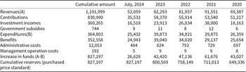
The NPF accumulates contributions and investment profits. Table 1 shows the detailed information on revenues, expenditures, and reserves of the NPF. According to Table 1, as of July 2024, the fund stands at 1,192 trillion KRW, with 827 trillion KRW in reserves after expenses.Footnote 5 With annual contributions exceeding 50 trillion KRW and annual benefits exceeding 25 trillion KRW, total fund growth surpasses 40 trillion KRW annually. The fund is mainly invested in financial assets (99.9%), with returns influenced by market fluctuations. The average return from the operation of the NPF from 1988, when the fund was established, until the end of 2023 was 5.92%, while the average return from 2021 to 2023 was lower at 5.04%. In July 2024, total returns reached 9.88%, driven by strong performance in foreign stocks (19.6%) and bonds (9.07%). The NPF is projected to grow to 1,755 trillion KRW by 2040.
Revenues, expenditures, and reserves of the National Pension Fund. (Unit: billion KRW)

Table 1 Long description
The table reports National Pension Fund revenues, expenditures, net fund increase, and cumulative reserves, with figures shown for July 2024, each year from 2020 to 2023, and cumulative totals in billion KRW. Cumulative revenues total 1,191,999, driven mainly by contributions at 830,990 and investment income at 360,265, while government subsidies are minimal at 744. Cumulative expenditures total 364,803, dominated by benefits at 352,558; administrative costs are 12,053 and management operation costs are 192. In every year shown, revenues are higher than expenditures, producing annual fund increases of 43,027 in 2020, 61,676 in 2021, 47,136 in 2022, 42,420 in 2023, and 26,628 for July 2024. Revenues peak in 2021 at 91,551 and then decline to 82,293 in 2023 and 52,059 by July 2024, while expenditures rise from 26,359 in 2020 to 39,873 in 2023 before reaching 25,432 by July 2024. Cumulative reserves at purchased-price basis increase each year from 649,336 in 2020 to 711,013 in 2021, 758,149 in 2022, 800,569 in 2023, and 827,197 by July 2024. July 2024 values represent a partial year, so comparisons with full-year totals should be made cautiously.
Notes: Government subsidies include direct subsidies, rents received from leasing out public corporation office buildings, and transfers. Management operation costs consist of personnel expenses, general expenses, and the costs of operating various projects. All values are in units of billion KRW.
2.2. Data description
In this section, we describe the data and variables we use in this paper. We use three main variables of interest in the analysis of the NPS: total contributions, total benefits, and the rate of return on pension funds (rate of return). Total contributions are mostly made up of funds paid toward the fund by the insured but may also include other minor revenues and government transfers. The rate of return on pension funds measures the returns from the investment side of the fund as a percentage of the invested amount. Total benefits include all outflows from the fund and consist mostly of the benefit payments made by the firm, but also include expenses of running the fund and other minor expenses.
We obtain data for quarterly contributions and annual total benefits from 2015 to 2023 from the national pension statistics provided by the Korea Statistical Information Service (KOSIS). The annual rate of return on pension investments is obtained from the Korean National Pension Service investment management website. Unfortunately, the National Pension Service only reports accrual accounting data after 2015, so we use data from 2015 to 2023 for the rate of return data in our analysis.
In what follows, we use VARs to estimate the response of flows in and out of the NPF in response to quarterly GDP shocks. However, in order to do so, we must convert our annual frequency data of total benefits and rate of return on pension investments to quarterly data. We use the Chow-Lin (Chow and Lin, Reference Chow and Lin1971) method to convert annual data of total benefits and rate of return on pension investments and convert them into quarterly variables. The Chow-Lin method interpolates low-frequency data into high-frequency data using related high-frequency variables, while also ensuring that the interpolated values are consistent with the annual data. To estimate the quarterly values of the rate of return, we use four related variables: return on corporate bonds, unemployment rates, log of the Korea Composite Stock Price Index (KOSPI), and log of KRW-USD exchange rates. To estimate the quarterly values of total benefit, we use the quarterly employment rate, log of real GDP, and CPI.
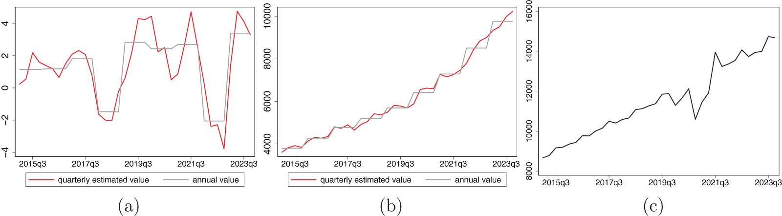
Figure 1 shows the NPS variables of interest in this paper. Panels (a) and (b) compare the quarterly estimated series with the annual values. Panel (a) shows the rate of return, and panel (b) shows contributions. Since the annual value is determined from the sum of values from four quarters, the gray line in panels (a) and (b) is the annual value, which is divided by four. As can be seen, our interpolated values are consistent with the annual values. Panel (c) shows the quarterly values for the contributions.
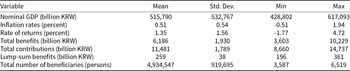
In the following section, we also include nominal GDP and inflation rates in our VAR analysis. Furthermore, we conduct analysis on the response of lump-sum benefits and the total number of beneficiaries to better understand the impulse response function of total benefits to GDP shocks. The variables lump-sum benefits and the total number of beneficiaries are obtained from the Korean National Pension Service Statistics. In Table 2, we show the summary statistics for the main variables used in our empirical analysis. We report the quarterly mean, standard deviation, minimum value, and maximum value of the variables for the period between the first quarter of 2015 and the last quarter of 2023.
NPS variables of interest. (a) Rate of return. (b) Total benefits. (c) Total contributions.

Figure 1 Long description
The image A showing a line graph titled Rate of return. The horizontal axis shows 2015q3, 2017q3, 2019q3, 2021q3, 2023q3. The left vertical axis shows negative 4, negative 2, 0, 2, 4. The right vertical axis shows 4000, 6000, 8000, 10000. A legend lists quarterly estimated value and annual value. Two lines are plotted. The quarterly estimated value line shows repeated rises and falls, including a drop below 0 around 2018 to 2019, a rise above 2 around 2019 to 2020, another rise above 2 around 2021, a drop below negative 2 around 2022 and a rise above 2 by 2023. The annual value line follows a stepped pattern with changes aligned to the same time period. The image B showing a line graph titled Total benefits. The horizontal axis shows 2015q3, 2017q3, 2019q3, 2021q3, 2023q3. The vertical axis label is not shown. The vertical axis shows 4000, 6000, 8000, 10000, 12000, 14000, 16000. A legend lists quarterly estimated value and annual value. Two lines are plotted. Both lines rise over time from near 4000 at the start toward near 16000 by 2023, with smaller increases and brief flattening around the middle years and larger increases after about 2020. The image C showing a line graph titled Total contributions. The horizontal axis shows 2015q3, 2017q3, 2019q3, 2021q3, 2023q3. The vertical axis label is not shown. The vertical axis shows 8000, 10000, 12000, 14000, 16000. One line is plotted. The line rises from near 8000 at the start to above 14000 by 2023, with a visible dip around 2020 to 2021 and a sharper rise around 2021. Across the three graphs, Total benefits and Total contributions show upward movement over time, while Rate of return shows alternating positive and negative values with larger swings around 2022 to 2023.
Summary statistics
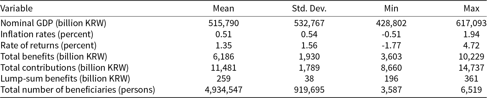
Table 2 Long description
Quarterly summary statistics are reported for key variables used in an empirical analysis from early 2015 through late 2023, including mean, standard deviation, minimum, and maximum. Nominal GDP has the largest scale and variability, with an average of 515,790 billion KRW and a range from 428,802 to 617,093. Inflation averages 0.51 percent and spans from minus 0.51 to 1.94, indicating occasional deflation. Rates of return average 1.35 percent and range from minus 1.77 to 4.72, showing both losses and gains. Total benefits average 6,186 billion KRW, compared with higher total contributions averaging 11,481 billion KRW; benefits range from 3,603 to 10,229 and contributions from 8,660 to 14,737. Lump-sum benefits are much smaller, averaging 259 billion KRW with values from 196 to 361. The total number of beneficiaries averages 4,934,547 with a standard deviation of 919,695, and the reported minimum and maximum are 3,587 and 6,519; because these extremes are far below the mean, the beneficiary counts may reflect a unit or reporting issue and should be interpreted cautiously.
Notes: In this table, we show the summary statistics for the main variables used in our empirical analysis. We report the quarterly mean, standard deviation, minimum value, and maximum value of the variables for the period between the first quarter of 2015 and the last quarter of 2023.
3. Impact of business cycles on NPS variables
In this section, we explore whether business cycle fluctuations impact the contributions, benefits, and rate of return of the NPS. We use a standard VAR model to study the impact of macroeconomic shocks on our NPS variables of interest. We estimate a three-variable VAR model including inflation rates and nominal GDP along with the dependent variable of interest. We use nominal GDP instead of real GDP as all NPS variables are also reported in nominal terms. We follow Ramey (Reference Ramey2011) in the sense that we estimate each of our NPS variables one-by-one together with the two macroeconomic variables. In Appendix A, we also report the results when we run all the variables together.
We use recursive identification using the following Cholesky ordering of the variables: inflation, log of nominal GDP, and log of the NPS variable. Inflation rates are placed first because we believe that it is reasonable to assume that inflation rates cannot be affected by contemporaneous changes in GDP or the NPS variables since prices, and therefore inflation, is thought to be somewhat sticky. The reason we put nominal GDP second is that we believe nominal GDP could be directly affected by an inflation shock, but it is plausible that it would take at least a quarter for shocks to the NPS variables to propagate through the economy and influence GDP. The NPS variables are liable to change in response to both contemporaneous changes in the inflation rate or GDP. To find the optimal lag length, we adopt both the Akaike and Bayesian information criteria for lag length selection. Both methods recommend using a lag of one, which we adopt.
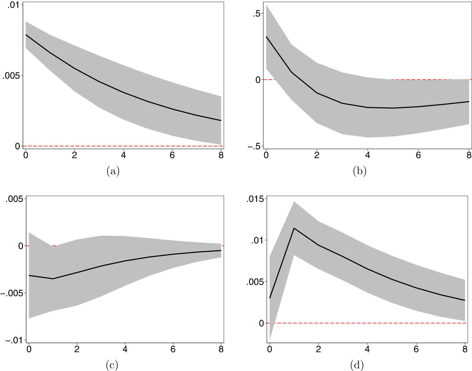
Figure 2 consolidates our results.Footnote 6 First, panel (a) of Figure 2 shows the impulse response of nominal GDP to a one standard deviation shock to nominal GDP. The estimated path of nominal GDP is standard, we see an immediate increase in nominal GDP of 0.7% and a slow decrease over the next 8 quarters showing that the shock to nominal GDP has some persistence. Because the estimated path of nominal GDP looks very similar in all three estimation results, we only depict the impulse response of nominal GDP once, the estimated response is for the case where we estimate the response of the rate of return.
Impulse response functions in response to a shock to NGDP. (a) Nominal GDP. (b) Rate of Return. (c) Total Benefits. (d) Total Contributions.
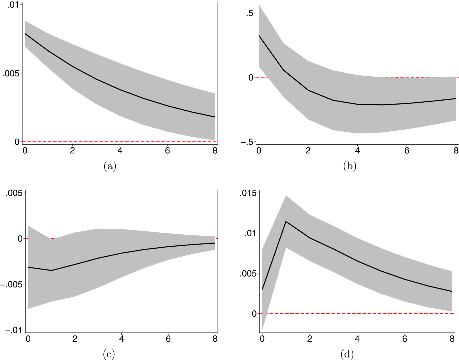
Figure 2 Long description
The image A showing a line graph labeled Nominal GDP. The horizontal axis shows 0 to 8. The vertical axis shows 0 to 0.01 with tick labels 0, 0.005, 0.01. A dashed horizontal reference line is at 0. A single curve starts near 0.008 at 0 and declines smoothly to about 0.002 at 8. A shaded band surrounds the curve across the full range. The image B showing a line graph labeled Rate of Return. The horizontal axis shows 0 to 8. The vertical axis shows negative 0.5 to 0.5 with tick labels negative 0.5, 0, 0.5. A dashed horizontal reference line is at 0. A single curve starts near 0.3 at 0, drops to near 0.05 at 1, crosses below 0 between 1 and 2, reaches about negative 0.2 around 4 to 5 and ends near negative 0.15 at 8. A shaded band surrounds the curve across the full range. The image C showing a line graph labeled Total Benefits. The horizontal axis shows 0 to 8. The vertical axis shows negative 0.01 to 0.005 with tick labels negative 0.01, negative 0.005, 0, 0.005. A dashed horizontal reference line is at 0. A single curve starts near negative 0.003 at 0, dips slightly near 1, then rises gradually, approaching 0 by 8. A shaded band surrounds the curve across the full range. The image D showing a line graph labeled Total Contributions. The horizontal axis shows 0 to 8. The vertical axis shows 0 to 0.015 with tick labels 0, 0.005, 0.01, 0.015. A dashed horizontal reference line is at 0. A single curve starts near 0.003 at 0, rises to a peak near 0.011 around 1, then declines steadily to about 0.003 by 8. A shaded band surrounds the curve across the full range.
In panel (b), we show the impulse response of the rate of return of NPS investments in response to a one standard deviation shock to GDP. The right side of the impulse-response function shows the rate of return on the NPF response to the nominal GDP. The rate of return increases immediately by 0.32 percentage points in response to a one standard deviation shock to nominal GDP, but then falls over the next four quarters. In fact, five quarters after the initial GDP shock, the impulse response function of the rate of return becomes significantly negative when we use one standard deviation confidence intervals. This pattern can arise because while a positive shock to nominal GDP may initially increase asset prices and thus raise returns, over time the heightened price of assets will imply that the returns that the NPS can expect from their assets will fall.Footnote 7
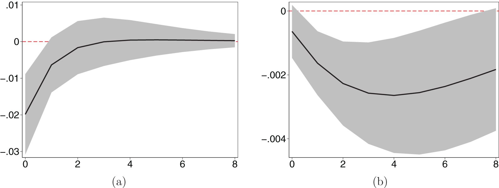
Panel (c) of Figure 2 shows the impulse response function of the log of total benefits. The response of benefits payout is relatively mitigated compared to rate of return or contributions. This is to be expected as benefits payout from funds will be made regardless of short-run economic conditions. However, we do see a slight decrease in benefits paid after one quarter and a gradual increase in the point estimates thereafter until the response converges to close to zero after 8 quarters. This can be explained by the fact that while repeated benefits payments are removed from business cycle considerations, one-time payouts where potential recipients claim their entire dues at once, may be related to the state of the economy. Furthermore, during economic expansions, people may delay retirement so that the number of beneficiaries decline. In Figure 3, we show that the impulse response functions for lump-sum benefits withdrawals and the log number of beneficiaries decrease in response to a positive shock to GDP. These impulse response functions are estimated by adding lump-sum withdrawals and the number of beneficiaries, respectively, as the last variable of the previously described VAR. The figures show that lump-sum benefits decrease by approximately 2% initially before gradually converging to zero.Footnote 8 The log number of beneficiaries show a persistent decline, and at its lowest point, four quarters after the initial shock, declines by approximately 0.25%.
Impulse response functions of benefits components. (a) Lump-sum Benefits. (b) Number of Beneficiaries.

Figure 3 Long description
The image A showing a line graph with a shaded band around the line and a dashed horizontal reference line at 0. Text below the graph: Lump-sum Benefits. The horizontal axis shows 0, 2, 4, 6, 8. The vertical axis shows 0.01, 0, minus 0.01, minus 0.02, minus 0.03. The plotted line starts near minus 0.02 at 0, rises to about minus 0.006 at 1, rises to about minus 0.001 at 2, reaches about 0 at 3, stays near 0 from 4 through 8. The image B showing a line graph with a shaded band around the line and a dashed horizontal reference line at 0. Text below the graph: Number of Beneficiaries. The horizontal axis shows 0, 2, 4, 6, 8. The vertical axis shows 0, minus 0.002, minus 0.004. The plotted line starts near minus 0.001 at 0, declines to about minus 0.0017 at 1, declines to about minus 0.0023 at 2, declines to about minus 0.0026 at 3, reaches about minus 0.0027 at 4, then rises to about minus 0.0026 at 5, about minus 0.0025 at 6, about minus 0.0023 at 7 and about minus 0.0020 at 8. Both graphs use the same horizontal axis tick labels from 0 to 8 and include a dashed reference line at 0, with the plotted lines shown with shaded bands.
Panel (d) of Figure 2 shows the impulse response function for the log of total contributions in response to a shock to nominal GDP. The estimated impulse response function illustrates that the contributions are very sensitive to business cycle fluctuations. A one standard deviation shock of nominal GDP increases total contributions by 1.1% one quarter after the initial shock, and the effect is persistent with residual effects lasting for over 8 quarters. We expect contributions to be sensitive to business cycle volatility as contributions are directly tied to employment and wages, which will fluctuate with GDP. Panel (d) shows that this is indeed the case.
All in all, our results show that the flow in and out of the NPF of Korea is susceptible to the short-run economic fluctuations of the Korean economy. Furthermore, considering the relatively short time span until the expected depletion, we believe that this implies that one can no longer safely ignore the business cycle implications in the forecast of funds and the impact it may have on its value and depletion. Therefore, in the following section, we attempt to augment the official projections of the NPF of Korea conducted by the National Pension Financial Estimation Expert Committee and simulate how accounting for short-run volatility may influence the projections of funds and forecasts about its depletion date.
4. Short-run volatility and NPF projections
4.1. Baseline projections
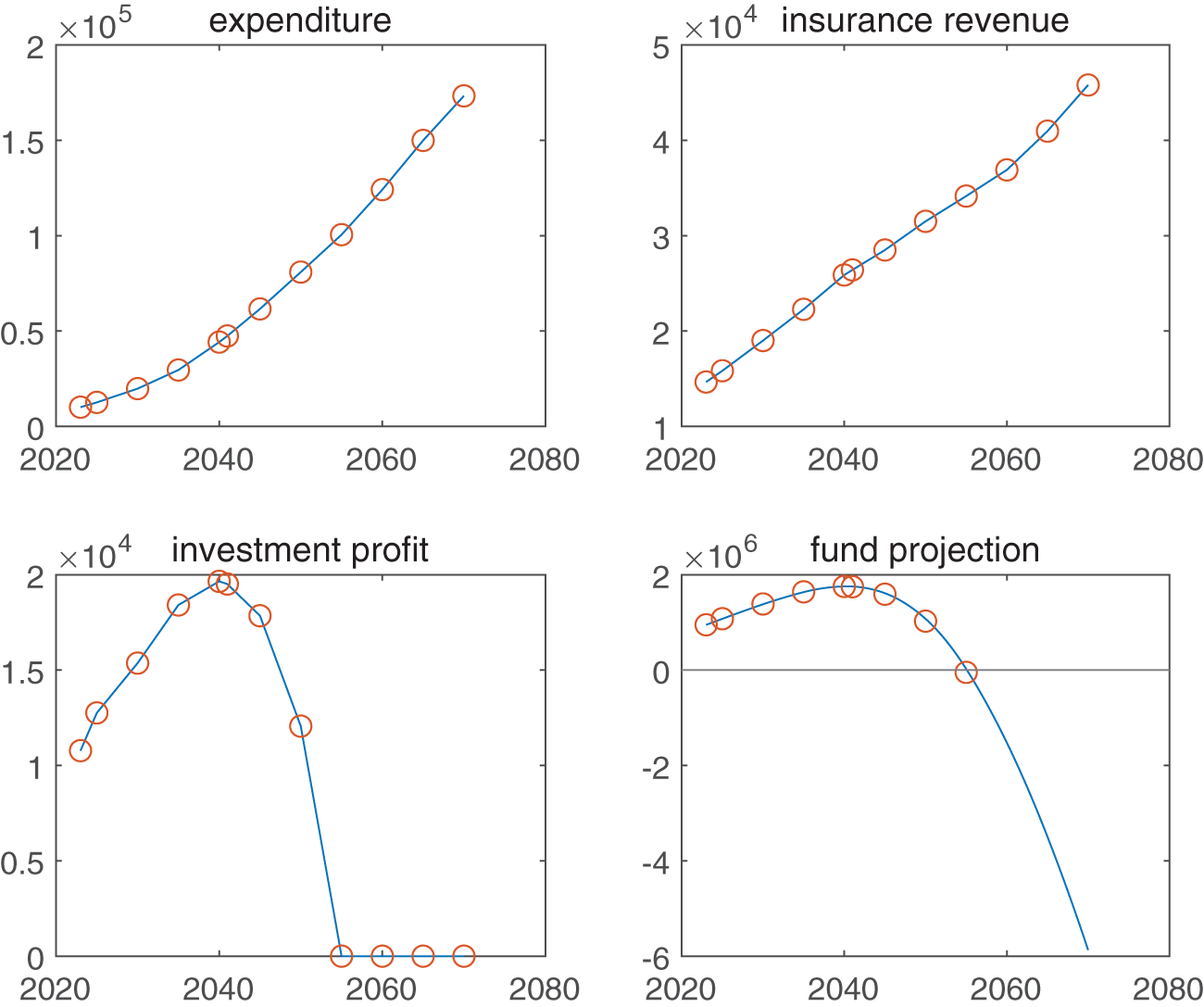
To analyze the effects of short-run fluctuations on the National Pension outlook, we first need to reconstruct the baseline projections conducted by the National Pension Financial Estimation Expert Committee in their report ‘2023 National Pension Financial Projection: Long-Term Financial Projection of the National Pension Fund Financial Estimate Expert Committee (2023)’ (henceforth NPFP). Since this report only provides the projections for select years, we interpolate the fund forecast values for each quarter using linear interpolation based on the reported estimates of contributions, benefits, and investment profit amounts (not rate of returns).
Figure 4 shows the projections of each variable for each quarter. The first 3 panels of Figure 4 show the quarterly values of expenditures, insurance revenue, and investment profits. The red circles show the reported values from the NPFP, and the blue lines show the interpolated values. The last panel then depicts the fund balance projections calculated as follows:
 \begin{equation}
Fund~ Balance_ t = Fund~ Balance_{t-1} + Contribution_t + Investment~ profit_t - Benefit_t~
\end{equation}
\begin{equation}
Fund~ Balance_ t = Fund~ Balance_{t-1} + Contribution_t + Investment~ profit_t - Benefit_t~
\end{equation}where  $t$ is from 2020 to 2060. The blue line shows the computed values of the fund balance and the red circles show the reported values in the NPFP. As can be seen in the fund projections, our linear interpolation method does an excellent job of recreating the fund balance values of the official projections. Therefore, we use these values as our baseline projection in our simulations going forward.
Projections of NPF variables.

Figure 4 Long description
The image A showing a line graph titled expenditure. The horizontal axis shows 2020 to 2080. The vertical axis shows 0 to 2 with the scale times 10 superscript 5. Plotted points follow an increasing curve from about 0.1 at about 2022, about 0.12 at about 2024, about 0.2 at about 2030, about 0.3 at about 2035, about 0.45 at about 2040, about 0.6 at about 2045, about 0.8 at about 2050, about 1.0 at about 2055, about 1.25 at about 2060, about 1.5 at about 2065 and about 1.75 at about 2070. The image B showing a line graph titled insurance revenue. The horizontal axis shows 2020 to 2080. The vertical axis shows 1 to 5 with the scale times 10 superscript 4. Plotted points rise from about 1.5 at about 2022, about 1.6 at about 2024, about 1.9 at about 2030, about 2.2 at about 2035, about 2.6 at about 2040, about 2.8 at about 2045, about 3.1 at about 2050, about 3.4 at about 2055, about 3.7 at about 2060, about 4.1 at about 2065 and about 4.6 at about 2070. The image C showing a line graph titled investment profit. The horizontal axis shows 2020 to 2080. The vertical axis shows 0 to 2 with the scale times 10 superscript 4. Plotted points increase from about 1.1 at about 2022 to about 1.3 at about 2025, about 1.55 at about 2030, about 1.85 at about 2035 and about 2.0 at about 2040, then decrease to about 1.8 at about 2045 and about 1.2 at about 2050. Points at about 2055, 2060, 2065 and 2070 lie on 0. The image D showing a line graph titled fund projection. The horizontal axis shows 2020 to 2080. The vertical axis shows negative 6 to 2 with the scale times 10 superscript 6. A horizontal line is drawn at 0. Plotted points are about 1.0 at about 2022, about 1.1 at about 2024, about 1.3 at about 2030, about 1.5 at about 2035, about 1.6 at about 2040, about 1.5 at about 2045, about 1.0 at about 2050 and 0 at about 2055. The curve continues downward to about negative 6 at about 2070.
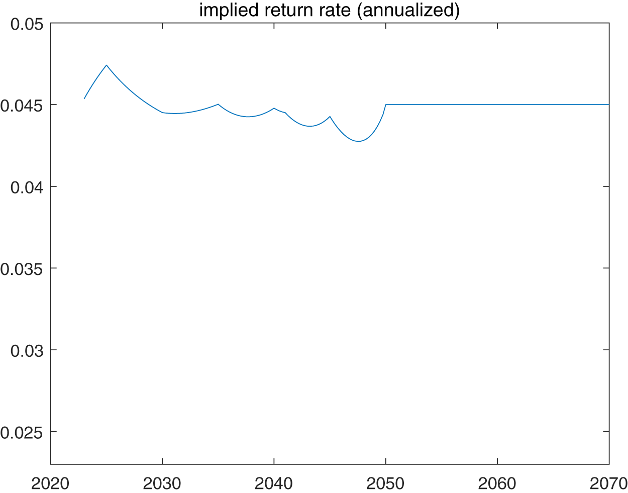
In addition, we construct the implied rate of returns by dividing the investment profits by the fund balance projections until depletion, as shown in Figure 5. Between the last projection before depletion in 2050 and depletion in 2055, we find that there is a precipitous drop in the implied rate of return on investments until depletion. We believe that this drop occurs due to interpolation and is not a fundamental phenomenon of fund dynamics. Therefore, for these periods we impute the average value of rate of return of 4.5% in our analysis. We also impute the value of 4.5% for all years after the expected depletion of funds in the benchmark projections, when we are simulating the effects of business cycles and of changing policy. We show the imputed values as well as all the values for each year in Figure 5.
Implied rate of return.

Figure 5 Long description
The graph title reads implied return rate (annualized). The x-axis shows years from 2020 to 2070, with labeled ticks at 2020, 2030, 2040, 2050, 2060 and 2070. The y-axis shows values from 0.025 to 0.05, with labeled ticks at 0.025, 0.03, 0.035, 0.04, 0.045 and 0.05. A single line starts slightly above 0.045 shortly after 2020, rises to a peak below 0.05 in the mid 2020s, then declines to just below 0.045 around 2030. The line then fluctuates around the 0.045 level through the 2030s and 2040s, dipping to a low point below 0.045 in the late 2040s. Around 2050, the line reaches 0.045 and becomes a horizontal line at 0.045 through 2070.
4.2. Simulating short-run fluctuations
We now discuss how we simulate the effect of short-run fluctuations on the flow of funds in and out of the NPF and consequently the value of the fund around the baseline deterministic projections. With short-run volatility, the path of fund balances will fluctuate around the deterministic projection. To model these fluctuations, we first simulate the GDP fluctuations around its trend value by assuming that GDP deviations follow an AR(1) process:
 \begin{equation}
\widehat{lnGDP}_t=\rho \widehat{lnGDP}_{t-1}+\epsilon_t.
\end{equation}
\begin{equation}
\widehat{lnGDP}_t=\rho \widehat{lnGDP}_{t-1}+\epsilon_t.
\end{equation}where 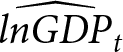 $\widehat{lnGDP}_t$ denotes the log deviation of GDP around its trend. We estimate the autocorrelation coefficient $\rho$ using Korean quarterly economic data from 2000 to 2023 and set its value to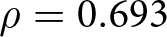 $\rho = 0.693$. We assume that the innovations $\epsilon_t$ are drawn from an i.i.d normal distribution with standard deviation equal to 1%, $\epsilon_t \sim N(0,0.01^2)$, which is equal to the average standard deviation of nominal GDP volatility in Korea.
Then, we multiply the estimated impulse response function(IRF) coefficients from the VAR analysis conducted in Section 3 for each variable  $i\in\{contributions, benefits,$ $ rate~ of~ returns\}$ to the log GDP deviations, in order to get the percent deviation of the variable $i$ due to changes in GDP. Specifically, we compute:
 \begin{equation}
M_{i,t} = \sum_{s=0}^{7} \beta_{i,s} \times \widehat{lnGDP}_{t-s}
\end{equation}
\begin{equation}
M_{i,t} = \sum_{s=0}^{7} \beta_{i,s} \times \widehat{lnGDP}_{t-s}
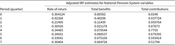
\end{equation}where  $\beta_{i,s}$ is the IRF coefficient of variable $i$ at horizon $s$, to get the percent deviation $M_{i,t}$ of the variable $i$ due to changes in GDP. The IRF coefficients used here are calculated as the estimated IRF values of the NPS variables to GDP shocks divided by the initial IRF value of GDP to the same shock, and IRF values over a period of eight quarters (two years) are applied. For example, in the case of contributions, the estimated IRF values of contributions are divided by the initial IRF value of GDP to derive the corresponding coefficients. The IRF values of each variable used in the analysis are summarized in Table 3. Furthermore, in the simulation, the impact of GDP fluctuations on investment profit is not directly estimated. Instead, the rate of return on fund assets is first computed, and then investment profit is derived by multiplying this rate by the previous period’s fund balance. Therefore, the key estimated variable representing volatility of investment profit is the rate of return on funds.
Adjusted IRF estimates for National Pension System variables
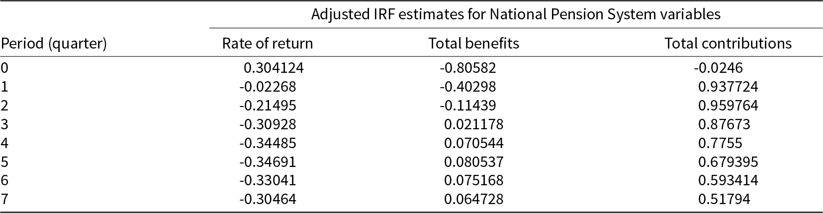
Table 3 Long description
Adjusted impulse-response estimates are listed by quarter from 0 to 7 for three National Pension System variables: rate of return, total benefits, and total contributions. The rate of return starts positive at 0.304 in quarter 0, turns slightly negative in quarter 1, and stays negative through quarter 7, reaching its lowest point around minus 0.347 in quarter 5 before edging up to minus 0.305 by quarter 7. Total contributions are near zero and slightly negative at quarter 0, then rise sharply to about 0.938 in quarter 1 and peak near 0.960 in quarter 2, followed by a steady decline to about 0.518 by quarter 7. Total benefits begin strongly negative at about minus 0.806 in quarter 0 and become less negative each quarter, crossing into small positive values by quarter 3 and peaking near 0.081 in quarter 5, then easing to about 0.065 by quarter 7. Overall, contributions respond quickly and then fade, returns show a sustained negative response after the initial quarter, and benefits move from negative to modestly positive over time. Values are coefficients intended for use in deviation calculations under GDP fluctuations, so they indicate direction and relative magnitude rather than direct levels.
Notes: This table shows the IRF coefficients of the rate of returns, contributions, and benefits that are used to calculate the deviations from the deterministic projections when facing GDP fluctuations. We use a period of eight quarters (two years) in the analysis.
Then we multiply the value  $M_{i,t}$ to the value of the variable in the baseline projection (which we denote $\bar{Y}_{i,t}$) to get the expected level change of variable $\hat{Y}_{i,t} = \bar{Y}_{i,t} \times M_{i,t}$. Finally, we get the simulated projection values taking the GDP fluctuations into account by adding the expected level change to the benchmark as follows:
 \begin{equation}
Y_{i,t} = \bar{Y}_{i,t} + \hat{Y}_{i,t}.
\end{equation}
\begin{equation}
Y_{i,t} = \bar{Y}_{i,t} + \hat{Y}_{i,t}.
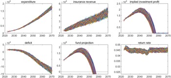
\end{equation} We simulate the path of GDP and consequently the path of the NPS variables  $Y_{i,t}$ 50,000 times. Figure 6 shows the different paths of the NPS variables and the fund projection can take for 5,000 of such simulations. As can be seen in Figure 6 there can be a wide range of outcomes depending on the fluctuations of GDP. Depending on the path of GDP the depletion of funds can be delayed or expedited.
Simulated paths of Nation Pension Fund projections.

Figure 6 Long description
The line graphs are arranged in a grid of six sub-images. Top-left line graph title: expenditure. The horizontal axis shows years from 2020 to 2070. The vertical axis shows values from 0 to 2 with a multiplier note of 10 superscript 5. Many lines rise over time, starting near 0 around 2020 and reaching near 2 by 2070. Top-middle line graph title: insurance revenue. The horizontal axis shows years from 2020 to 2070. The vertical axis shows values from 0 to 6 with a multiplier note of 10 superscript 4. Many lines rise over time, starting near 0 around 2020 and reaching around 4 to 5 by 2070. Top-right line graph title: implied investment profit. The horizontal axis shows years from 2020 to 2070. The vertical axis shows values from 0 to 2.5 with a multiplier note of 10 superscript 4. Many lines rise from near 0 around 2020 to a peak around 2.0 to 2.5 between about 2035 and 2045, then fall toward 0 by about 2060 to 2070. Bottom-left line graph title: deficit. The horizontal axis shows years from 2020 to 2070. The vertical axis shows values from negative 15 to 0 with a multiplier note of 10 superscript 4. Many lines start near 0 around 2020 and move downward over time, reaching around negative 12 to negative 15 by 2070. Bottom-middle line graph title: fund projection. The horizontal axis shows years from 2020 to 2070. The vertical axis shows values from 0 to 2 with a multiplier note of 10 superscript 5. Many lines rise from near 0 around 2020 to a peak near 1.5 to 2.0 between about 2035 and 2045, then fall toward 0 by about 2060 to 2070. Bottom-right line graph title: return rate. The horizontal axis shows years from 2020 to 2070. The vertical axis shows values from 0.035 to 0.045. Many lines fluctuate within this band across the full time range.
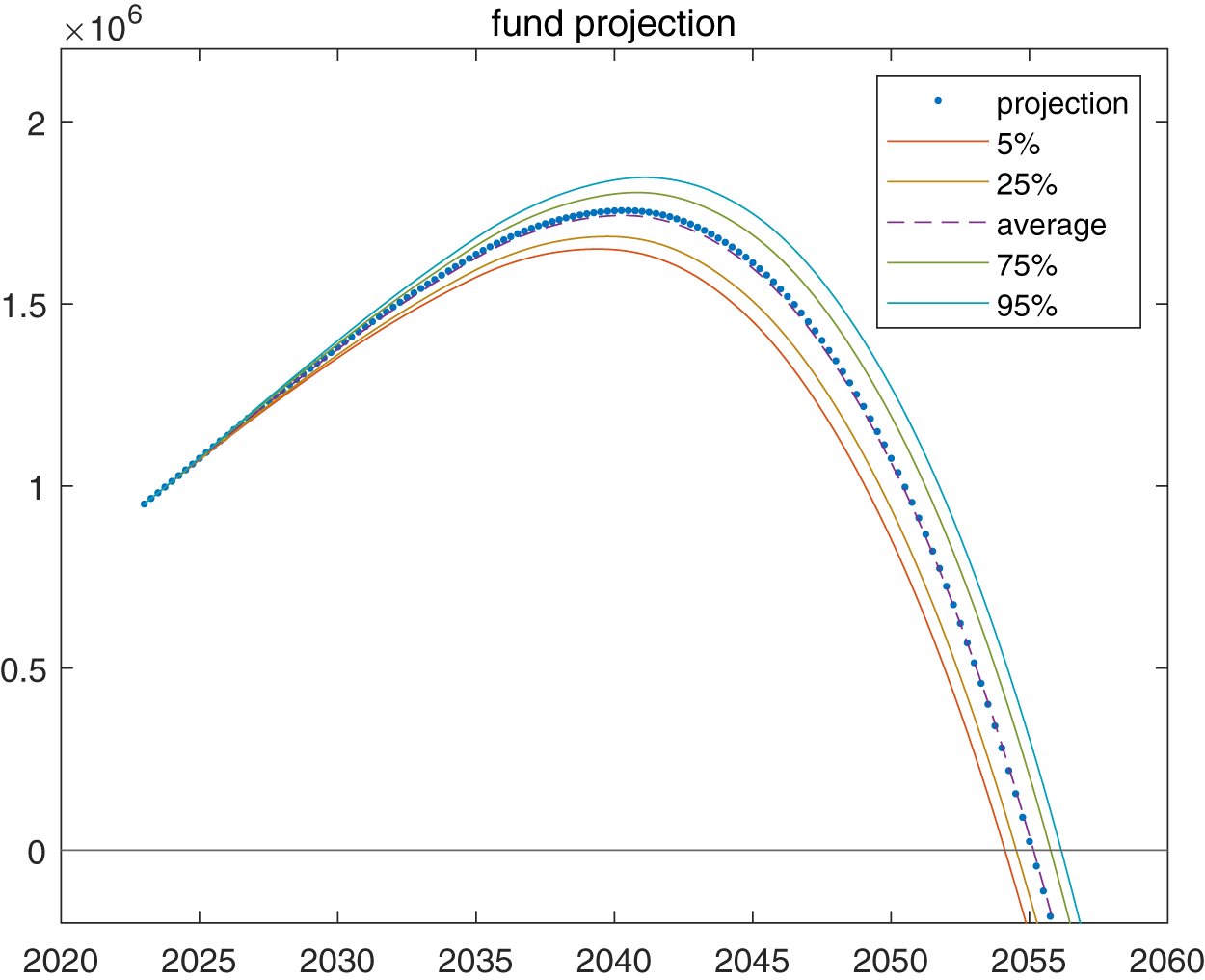
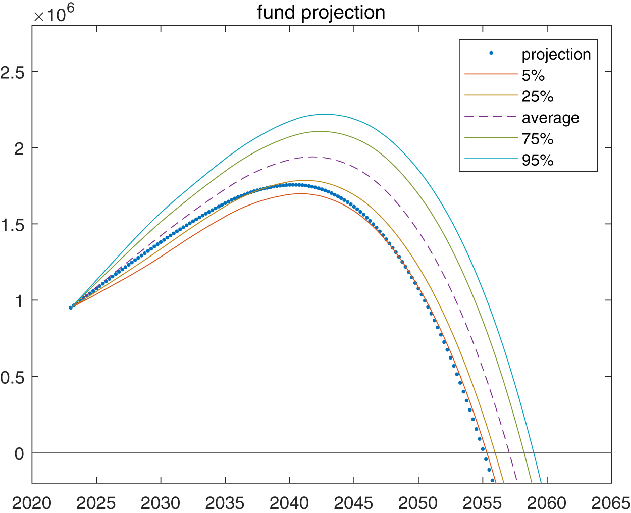
To make things clearer, Figure 7 summarizes the results for the fund projections. We show the average path of the simulations as well as the paths consisting of the average value of all paths in the top 95th percentile of projections, 75th percentile of projections, bottom 25th percentile and the bottom 5th percentile of projections. Although accounting for business cycle fluctuations introduces variability in the projected depletion dates, the range remains close to the deterministic projections. The bottom 5th percentile suggests the fund could be depleted one year earlier than the baseline forecast, in 2054 rather than 2055, while the top 5th percentile indicates depletion one year later in 2056. Despite incorporating GDP fluctuations, the deviation from the baseline remains relatively small. This is likely due to the fact that even with significant differences in fund value when the fund’s assets are large, the gap between the simulation and the baseline forecasts narrows as depletion approaches. Nevertheless, considering GDP fluctuations does result in small but noticeable variations in the projected depletion dates.
Summary of simulated paths of Nation Pension Fund projections.

Figure 7 Long description
Fund projection Legend: projection; 5 percent; 25 percent; average; 75 percent; 95 percent. Horizontal axis: 2020 to 2060. Vertical axis: 0 to 2 with a scale note times 10 superscript 6. Line and marker styles: projection is shown with dot markers; average is shown with a dashed line; 5 percent, 25 percent, 75 percent and 95 percent are shown with solid lines. Visible axis tick labels. Horizontal axis tick labels: 2020, 2025, 2030, 2035, 2040, 2045, 2050, 2055, 2060. Vertical axis tick labels: 0, 0.5, 1, 1.5, 2. Data values: no numeric coordinate pairs are explicitly labeled on the plotted lines or markers. Overall shape of all series: values rise from the mid 2020s to a peak around 2040 to 2042, then decline steeply toward the mid 2050s. Relative ordering across percentiles: the 95 percent line is highest, followed by 75 percent, average, 25 percent and 5 percent. Projection markers: the dot markers follow a path close to the average line from the mid 2020s through the early 2050s. Approximate peak region using the vertical axis scale note times 10 superscript 6. Around 2040 to 2042: 95 percent is just under 2 times 10 superscript 6; 75 percent is slightly below the 95 percent line; average is around 1.7 to 1.8 times 10 superscript 6; 25 percent is below the average; 5 percent is the lowest near about 1.6 to 1.7 times 10 superscript 6. Approximate low region near the mid 2050s: all lines approach the 0 level around 2055 to 2056, with the 5 percent and 25 percent lines reaching the 0 level earlier than the 75 percent and 95 percent lines.
4.3. An increase in the target rate of return
In this section, we study what happens to the path of funds when the policy target rate of return is increased. To increase the rate of return on the fund operations, it is inevitable that one must raise the riskiness of the investment portfolio. The rate of return on assets is proportional to the risk, meaning that to achieve a higher return one must invest in riskier assets. Then, if the National Pension Service decides to increase the portfolio weight of high-risk assets, the volatility of the rate of return on funds would increase. If so, one can easily expect that it could accelerate the depletion timeline in downside scenarios of the NPF forecast simulations. In this paper, we study the effect of a raise in the target rate of return of 0.5%.
There exists extensive literature that includes how much volatility one must bear to raise 0.5% of asset return. In this study, we set 4% as the standard deviation increase in the rate of return for raising 0.5% of the expected return rate. This choice is based on the 0.125 Sharpe ratio value that Cheong et al. (Reference Cheong, Kim and Kim2023) estimate using data on the Korean stock market. This value is similar to the value computed based on conditional variance and expected return coefficients in Park et al. (Reference Park, Eom and Hahn2017). It is also similar to the results from other studies in the literature such as those by Kim (Reference Kim2009) and Ha and Kang (Reference Ha and Kang2014). In this study, we start the analysis assuming that the NPF asset is efficiently constructed, which means the increasing volatility required to raise the return rate is the same as the Sharpe ratio estimated in the Korean stock market.
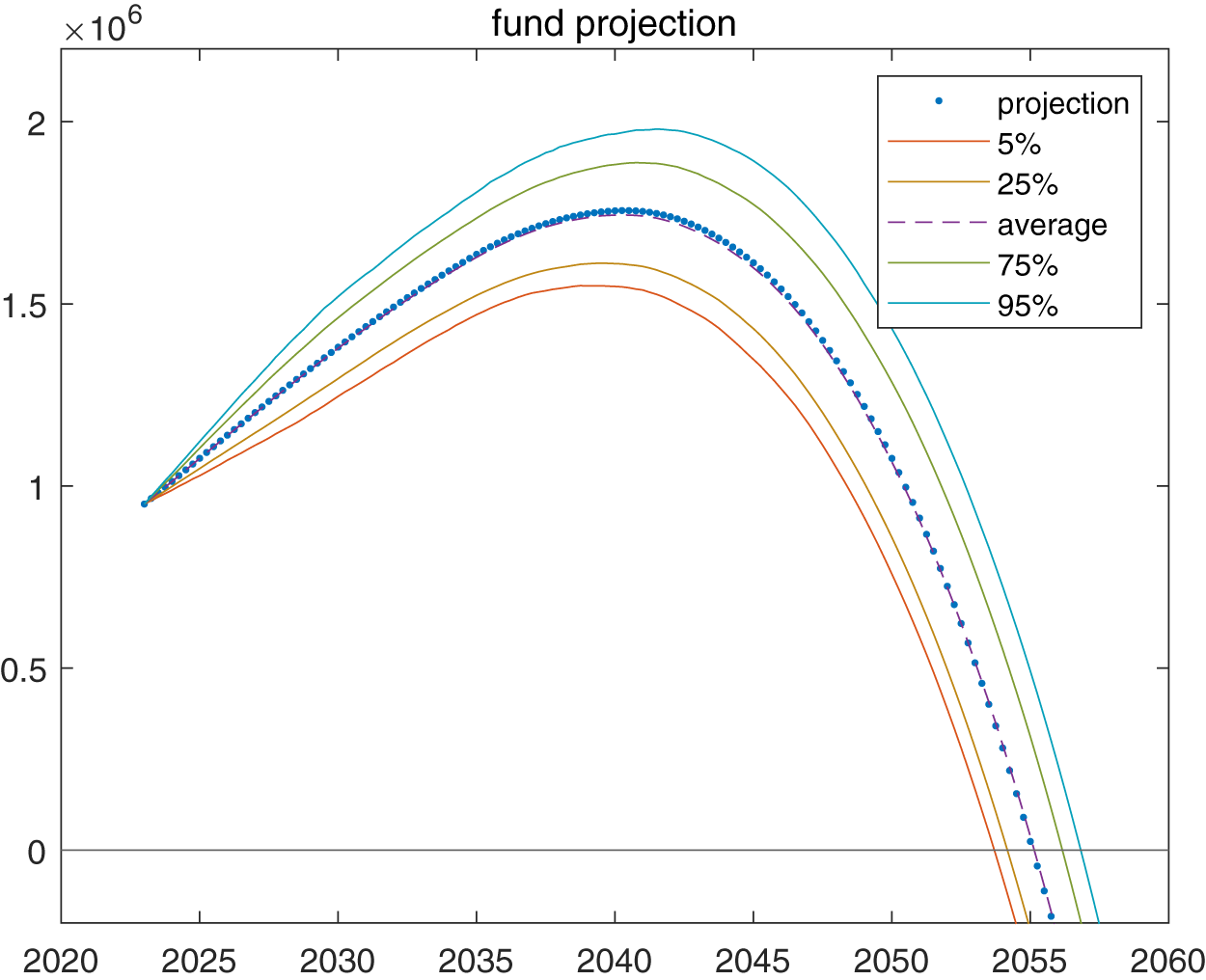
Before we explore the effect of a policy target rate increase, we first examine what happens when only the volatility of rate of return increases, without raising the expected rate of return. We increase the volatility by adding random noise of 4% to the rate of return of funds. Figure 8 shows how the fund asset forecast changes if the standard deviation of the rate of return on pension funds increases by 4%. The projected depletion date for the bottom 5th percentile is two years earlier than the deterministic projection, and the top 5th percentile is approximately two years delayed. Thus, it is plausible trying to increase the policy target could result in some outcomes that leaves the fund worse off than it otherwise would have experienced.
Summary of simulated paths of Nation Pension Fund projections with increased volatility.

Figure 8 Long description
The graph titled 'fund projection' displays projections from 2020 to 2060. The horizontal axis represents years and the vertical axis represents fund value in millions. The graph includes several lines: a dotted line for projection, solid lines for 5 percent, 25 percent, 75 percent and 95 percent percentiles and a dashed line for the average. The lines show a general rise to a peak around the early 2040s, followed by a steep decline toward zero in the mid-2050s. The 95 percent line is the highest and the 5 percent line is the lowest, indicating a widening spread over time. The peak occurs around 2045, with values approximately reaching 2 million. The graph illustrates the potential variability in fund projections over time.
In Figure 9, we show the results when we increase both the rate of return and the volatility of returns as discussed. According to Figure 9 when we raise the rate of returns on fund assets by 0.5%, the average depletion forecast of fund asset is pushed back to the year 2057. On the upside of the simulation, the variance of the depletion forecast is delayed by even more until the year 2059, and even the bottom 5th percentile of simulated projections have the fund becoming deleted at a date slightly later than the deterministic projection. This is because the effects of an increase in the rate of return dominates the effects of raising its volatility.
Summary of simulated paths of Nation Pension Fund projections with increased target rate of return and increased volatility.

Figure 9 Long description
The graph titled 'fund projection' displays multiple lines representing different percentiles and an average of fund projections over time. The horizontal axis is labeled with years ranging from 2020 to 2065. The vertical axis represents fund values in millions, ranging from 0 to 3 million. The legend identifies the lines as follows: projection (dotted line with markers), 5 percent (solid line), 25 percent (solid line), average (dashed line), 75 percent (solid line) and 95 percent (solid line). The graph shows an overall trend where all lines rise to a peak around the year 2040 and then decline towards 2065. The projection line starts at approximately 1 million in 2020, peaks at around 2.5 million in 2040 and declines to near zero by 2065. The 95 percent line is the highest throughout, while the 5 percent line remains the lowest. The average line follows a similar trend, peaking slightly below the 75 percent line. The lines are visually distinguished by different styles and colors, with the projection line marked by dots. This graph illustrates the projected fund values over time, highlighting differences in percentiles and average projections.
4.4. Sensitivity analysis
Finally, in the previous section, we assumed a Sharpe ratio value of 0.125, which was the value estimated by Cheong et al. (Reference Cheong, Kim and Kim2023) for the Korean stock market, to compute the amount of volatility increase we should expect in response to an increase in average returns. However, there may be various circumstances under which the appropriate Sharpe ratio value takes on a different value. For example, the large size of the NPF may imply that if it seeks a higher return through investments in smaller, riskier stocks and later seeks to sell these stocks, they may cause excess volatility in the market above and beyond what can currently be observed in the market. Furthermore, the NPF is rapidly increasing its overseas portfolio so the volatility associated with higher returns may not match Korean market figures. With overseas investments exchange rate effects must also be considered. In these cases the expected volatility increase may be underestimated.Footnote 9 Thus, in this section, we conduct simulations studying how altering the volatility response to an increase in the expected return will change the projections of the NPF. We consider three alternative scenarios chosen as follows.
First, we consider the extreme case in which the volatility increase is determined by the Sharpe ratio at the lower end of the estimates of the European countries, equal to 0.02.Footnote 10 This would imply that the volatility increases by 50 times the amount of increase in the rate of return. While this is admittedly an extreme case, it will be interesting to compare the extreme case with more realistic scenarios. The results of the simulation under this assumption are shown in panel (a) of Figure 10.
Sensitivity analysis of increasing the target rate of return.

Figure 10 Long description
The image contains three multi-line graphs labeled (a), (b) and (c), each titled 'fund projection'. The x-axis represents the year from 2020 to 2065 and the y-axis represents fund value in millions, scaled by 10 superscript 6. Each graph includes lines for projection, 5 percent, 25 percent, average, 75 percent and 95 percent. The projection line is dotted, the average line is dashed and percentile lines are solid. Graph (a) shows a peak around 2050, with the 95 percent line reaching approximately 5.5 million, while the 5 percent line peaks lower and declines to zero by 2065. Graph (b) has a similar pattern, peaking around 2045, with the 95 percent line reaching about 2.5 million. The lower percentiles decline to zero earlier. Graph (c) also peaks around 2045, with the 95 percent line reaching approximately 2.5 million. The lines show a rise to a mid-period peak followed by a decline, with lower percentiles reaching zero earlier and upper percentiles remaining higher longer.
In this scenario, in the bottom 95th percentile outcome the NPF runs out of funds seven years earlier than what the benchmark deterministic projection forecasts. In the bottom 75th percentile outcome the NPF runs out of funds four years earlier than currently expected. Thus, with added volatility there is considerable risk that raising the expected policy return may lead to an even faster depletion of funds. We note that there is also considerable upside to raising the expected policy return with greater volatility, if all goes well, the top 25th percentile outcome implies that the fund’s depletion is pushed back nearly ten years, and even further in the top 5th percentile of outcomes.
Next, we consider the case in which the bottom 25th percentile outcome is equivalent to the benchmark deterministic projection. The necessary increase in the volatility to achieve this is equivalent to 16 times the increase in the expected return. This would imply a Sharpe ratio of 0.0625, half of the value used in the main analysis of Section 4.3. The results of the simulation under this assumption are shown in panel (b) of Figure 10. We find that even if there is considerably more risk associated with increasing the expected return than we had originally assumed, in three-fourths of the cases the depletion date would still be later than what the current benchmark projection indicates. Furthermore, the downside of raising the policy target in this case seems to be also limited in the sense that, even in the worst 5th percentile of outcome, the depletion date is only expedited by approximately one year.Footnote 11
Lastly, we consider the case in which the volatility increase necessary to increase the expected return is smaller than the benchmark case of Section 4.3. For this simulation, we use the Sharpe ratio of 0.18, as estimated for the U.S. While this scenario is unlikely to be true, the exercise provides an interesting benchmark of what could theoretically be achieved if the NPF were able to invest in a way such that their expected return increases without causing too large of an increase in the volatility of their portfolio. This case is shown in panel (c) of Figure 10. As expected, in this case we find that even the very bad simulations outperform the benchmark deterministic projection.
5. Conclusion
In this paper, we explore the effects of short-run fluctuations on the projections of the NPS of Korea. We find that the flow of funds into and out of the NPF of Korea is sensitive to short-run fluctuations. However, when we incorporate these fluctuations in the flow of funds into the NPF projections, we find that the quantitative effects of additional volatility are modest. In addition, in our simulation analysis we find that raising the target rate of return on NPF investments delays the average projected date of depletion. Moreover, even the average projection in the bottom 5th percentile of bad outcomes, when we raise the target rate of return, has a depletion date further into the future than the average deterministic projection at current rates of return.
Therefore, our results may suggest that it would be beneficial for Korea, and similar countries that face depletion of pension funds in relatively short order, to raise their policy target rate of returns on their fund portfolio investments, even after considering the downsides that may be present due to greater volatility from riskier investments if one considers business cycle fluctuations.
Appendix A. 5 Variable VAR
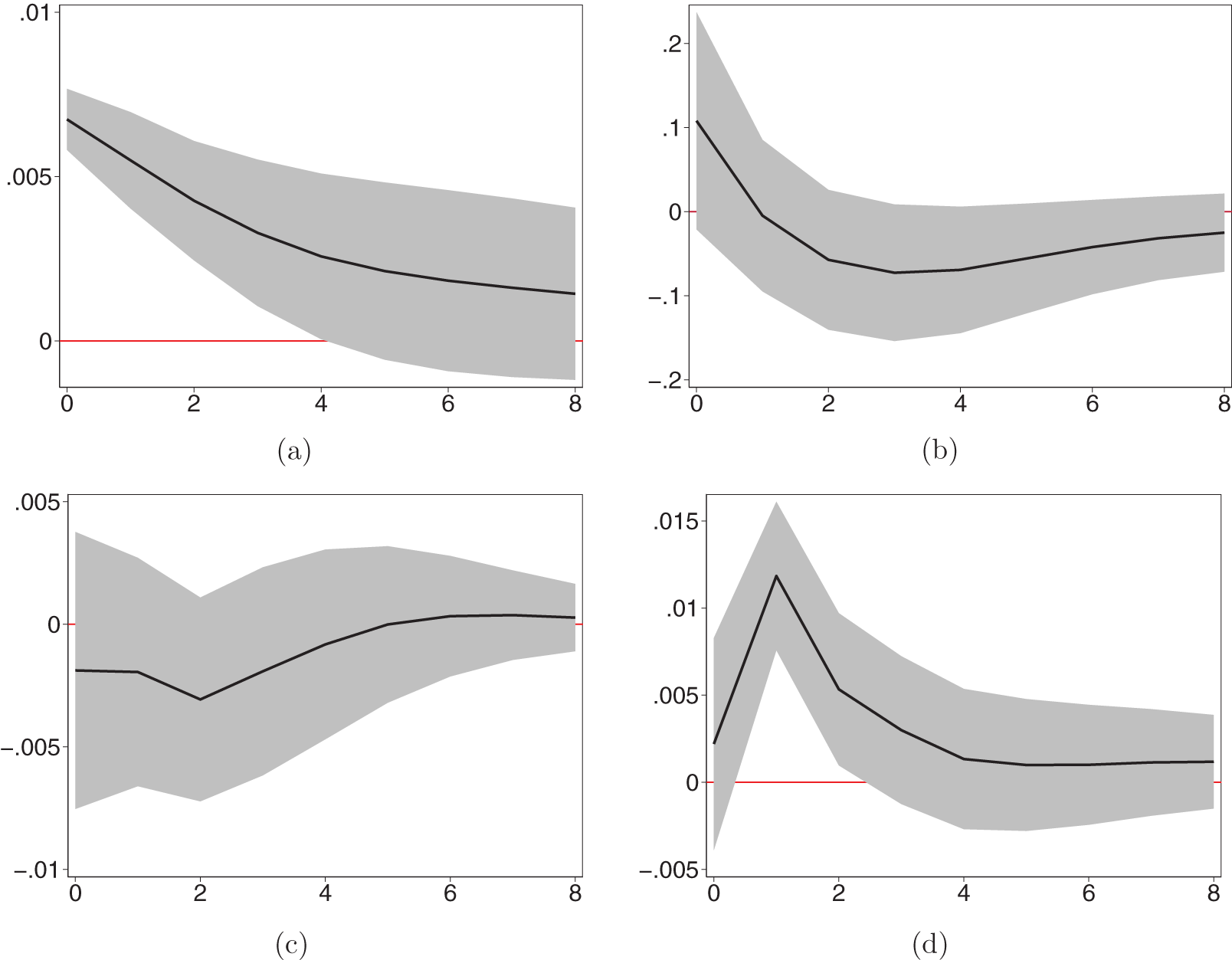
Figure A1 reports the VAR impulse response functions of the five variable VAR, estimated with inflation rate ordered first, nominal GDP second, and then the NPS variables in order of rate of return, total benefits, and total contributions. The estimated results look very similar to those in Figure 2 of the main text.
IRFs for five variable VAR. (a) Nominal GDP. (b) Rate of Return. (c) Total Benefits. (d) Total Contributions.

Figure A1 Long description
The image A showing a line graph labeled Nominal Gross Domestic Product. The horizontal axis shows 0 to 8. The vertical axis shows 0, 0.005 and 0.01. A line starts near 0.0065 at 0, declines to about 0.0045 at 2, about 0.0030 at 4, about 0.0020 at 6 and about 0.0015 at 8. A horizontal reference line is drawn at 0. A shaded band surrounds the line. The image B showing a line graph labeled Rate of Return. The horizontal axis shows 0 to 8. The vertical axis shows negative 0.2, negative 0.1, 0, 0.1 and 0.2. A line starts near 0.10 at 0, reaches about 0 at 1, declines to about negative 0.06 at 2, about negative 0.08 at 3, then rises to about negative 0.07 at 4, about negative 0.05 at 6 and about negative 0.03 at 8. A horizontal reference line is drawn at 0. A shaded band surrounds the line. The image C showing a line graph labeled Total Benefits. The horizontal axis shows 0 to 8. The vertical axis shows negative 0.01, negative 0.005, 0 and 0.005. A line is near negative 0.002 at 0 and 1, drops to about negative 0.003 at 2, rises to about negative 0.002 at 3, about negative 0.001 at 4, reaches about 0 at 5 and is slightly above 0 from 6 to 8 at about 0.0002 to 0.0004. A horizontal reference line is drawn at 0. A shaded band surrounds the line. The image D showing a line graph labeled Total Contributions. The horizontal axis shows 0 to 8. The vertical axis shows negative 0.005, 0, 0.005, 0.01 and 0.015. A line starts near 0.002 at 0, peaks near 0.012 at 1, declines to about 0.005 at 2, about 0.003 at 3, about 0.0015 at 4, about 0.0010 at 5 and stays near 0.0010 to 0.0012 from 6 to 8. A horizontal reference line is drawn at 0. A shaded band surrounds the line.
Appendix B. VAR coefficients
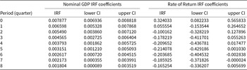
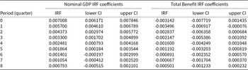
Tables B1, B2, and B3 show the IRF coefficients for the estimated VAR impulse response functions shown in Table 2.
IRF coefficients for the rate of return on National Pension Fund
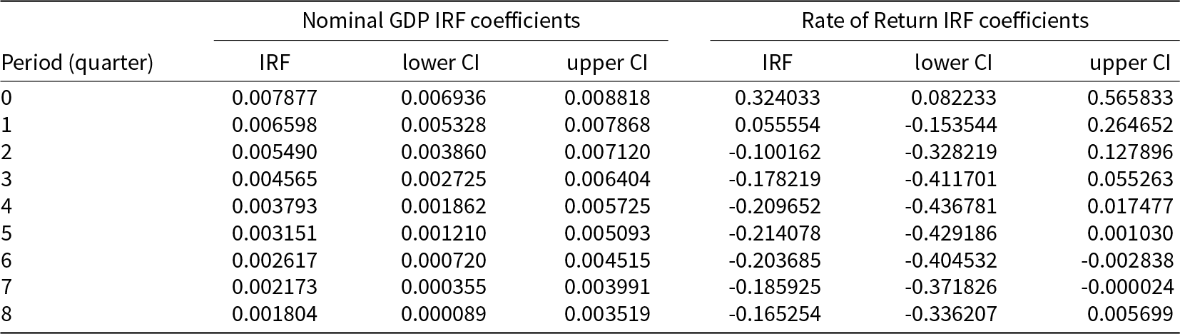
Table B1 Long description
The table reports impulse response coefficients for the National Pension Fund rate of return over quarters 0 through 8, with lower and upper bounds from a 68 percent confidence interval. For Nominal GDP, the response is positive in every period and declines steadily from about 0.0070 at quarter 0 to about 0.00079 by quarter 8. The Nominal GDP interval is fully above zero through quarter 5, then crosses zero from quarter 6 onward, indicating weaker statistical support later. For Total Benefits, the response is negative throughout, moving from about minus 0.00314 at quarter 0 to about minus 0.00050 by quarter 8. The Total Benefits interval crosses zero in most periods, except quarter 1 where it remains slightly below zero, suggesting limited precision outside that quarter. Overall, both responses diminish in magnitude over time, and later-quarter effects should be interpreted cautiously because the confidence intervals often include zero.
Notes: This table shows IRF coefficients corresponding to the rate of returns in Table 2. The lower CI and upper CI are estimated based on 68% confidence intervals.
IRF coefficients for total benefit
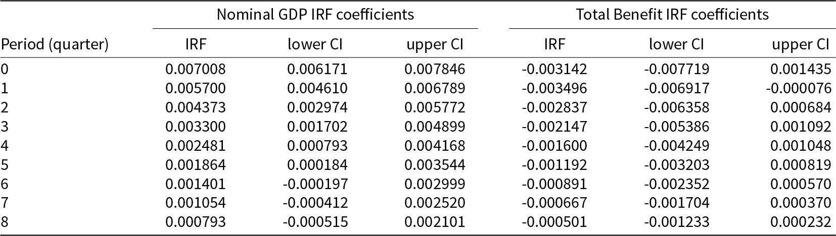
Table B2 Long description
The table reports quarterly impulse response coefficients for nominal GDP and for total benefit, each with lower and upper bounds from a 68 percent confidence interval. Nominal GDP is positive in every period, starting at 0.007008 in quarter 0 and declining steadily to 0.000793 by quarter 8. Its uncertainty band is fully above zero through quarter 5, then crosses zero from quarter 6 onward as the lower bound turns slightly negative. Total benefit is negative in every period, from minus 0.003142 at quarter 0 to minus 0.000501 at quarter 8, indicating the effect weakens toward zero over time. The total benefit interval includes zero in most quarters, but quarter 1 is entirely below zero with bounds from minus 0.006917 to minus 0.000076. Overall, nominal GDP shows a small, decaying positive response, while total benefit shows a small, decaying negative response, with statistical uncertainty increasing relative to the effect size at longer horizons.
Notes: This table shows IRF coefficients corresponding to the total benefits in Table 2. The lower CI and upper CI are estimated based on 68% confidence intervals.
IRF coefficients for total contribution
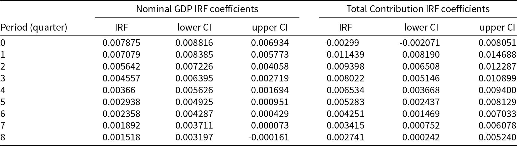
Table B3 Long description
The table reports impulse response coefficients by quarter for nominal GDP and for total contribution, each with lower and upper bounds from a 68 percent confidence interval. Nominal GDP starts near 0.0079 at quarter 0 and declines each quarter to about 0.0015 by quarter 8. Total contribution begins near 0.0030 at quarter 0 with an interval that crosses zero, then rises to its highest value around 0.0114 at quarter 1 with a fully positive interval. After quarter 1, total contribution decreases steadily from about 0.0094 at quarter 2 to about 0.0027 at quarter 8, with intervals remaining above zero from quarter 1 onward. Across quarters 1 through 8, total contribution coefficients are consistently larger than nominal GDP coefficients. Interpret the bounds as uncertainty ranges rather than exact limits, and note they reflect a 68 percent confidence level.
Notes: This table shows IRF coefficients corresponding to the total contributions in Table 2. The lower CI and upper CI are estimated based on 68% confidence intervals.



 Open access

