


1. Introduction
Arctic sea ice is an important component of the global climate system (Serreze and Meier, Reference Serreze and Meier2019) and plays a crucial role in the global ocean circulation (Sévellec and others, Reference Sévellec, Fedorov and Liu2017). In the context of climate change, Arctic sea ice has undergone a rapid decline during the past decades and hence, gains great attention from climate research and social industrial applications (Comiso and Hall, Reference Comiso and Hall2014; Meier and others, Reference Meier2014; Stroeve and Notz, Reference Stroeve and Notz2015). For example, the rapid decline of Arctic sea ice in recent years has spurred more commercial traffic through the Arctic routes with significantly reduced distance from Asia to Europe (Melia and others, Reference Melia, Haines, Hawkins and Day2017; Zhang and others, Reference Zhang, Hu and Dai2020). In the Central Arctic, the ocean is covered by close pack ice and compact pack ice, and the navigability is primarily controlled by the sea-ice thickness (SIT) and sea-ice concentration (SIC) along the route. Among all the sea-ice properties, SIT is important, because changes in its distribution can affect the ocean-atmosphere heat fluxes especially during the fall period (Kurtz and others, Reference Kurtz, Markus, Farrell, Worthen and Boisvert2011). However, until the 1990s, our knowledge of SIT distribution was hampered by the sparsity of observations except for some submarine records (Rothrock and others, Reference Rothrock, Yu and Maykut1999). Uotila and others (Reference Uotila2019) demonstrated the large differences of sea-ice volume (SIV) and SIT in ten ocean and sea-ice reanalysis products in their Polar Ocean Reanalyses (ORA) Intercomparison Project. With respect to the Ice Thickness Regression Procedure (Lindsay and Schweiger, Reference Lindsay and Schweiger2015) data in February–March, most of these products underestimate SIT to the north of the Canadian Arctic Archipelago (NOCAA) and the north of Greenland and the Fram Strait, but overestimate SIT over the Eurasian shelves. This exposes the lack of direct constraints on SIT, which is a common deficiency of all reanalysis products.
Estimating of the Arctic sea-ice extent (SIE) and SIT relies upon numerous geophysical parameters which could result in large uncertainties. In contrast to the successes of deriving SIC and SIE from satellite (Cavalieri and Parkinson, Reference Cavalieri and Parkinson2012), SIT retrieval still has large uncertainties (Kwok and Cunningham, Reference Kwok and Cunningham2015). With an assumption of hydrostatic equilibrium, SITs can be estimated from the freeboard measurements boarded on satellite altimeters, for example Envisat since 2002 (Connor and others, Reference Connor, Laxon, Ridout, Krabill and McAdoo2009; Hendricks and others, Reference Hendricks, Paul and Rinne2018), ICESat since 2003 (Kwok and others, Reference Kwok2009) and CryoSat-2 since 2010 (Ricker and others, Reference Ricker, Hendricks, Helm, Skourup and Davidson2014). The estimated SITs still have large uncertainties, which come along with the utilization of the snow depth (Warren and others, Reference Warren1999) and the assumption of hydrostatic equilibrium. Since 2010, the thickness for thin ice (<1.0 m) can be retrieved by the brightness temperature observations measured by Soil Moisture and Ocean Salinity (SMOS) satellite (Kaleschke and others, Reference Kaleschke2010; Tian-Kunze and others, Reference Tian-Kunze2014), although the SMOS thickness data may suffer from inaccurate boundary conditions introduced by the sea ice-ocean model (Tian-Kunze and others, Reference Tian-Kunze2014). Exploiting the complementary characters of CryoSat-2 and SMOS SITs, Ricker and others (Reference Ricker2017) further merged them together into an Arctic-wide SIT dataset, CS2SMOS. Retrieving SIT from satellite assumes that the peak reflection in the radar altimetry data originates from snow/ice interface (Laxon and others, Reference Laxon, Peacock and Smith2003). However, it is difficult to separate the echoes from the open water and melt ponds during the melting season, all satellite-derived SITs are only available in the cold seasons, from October to March.
In recent years, the satellite observed SIC and SIT have been assimilated into ice-ocean coupled models and the results showed promising improvements in reconstructing the time series of Arctic SIT (Yang and others, Reference Yang2014, Reference Yang, Losch, Losa, Jung and Nerger2016; Posey and others, Reference Posey2015; Xie and others, Reference Xie, Counillon, Bertino, Tian-Kunze and Kaleschke2016, Reference Xie, Counillon and Bertino2018; Mu and others, Reference Mu2018a). In particular, a widely used sea-ice reanalysis, TOPAZ4, is accessible through the Copernicus Marine Environment Monitoring Service (CMEMS; https://resources.marine.copernicus.eu) portal with the product id of ARCTIC_REANALYSIS_PHYS_002_003. This reanalysis product is extended yearly, based on a coupled ocean and sea-ice assimilation system. In this system, the hybrid coordinate ocean model (HYCOM; Chassignet and others, Reference Chassignet, Chassignet and Verron2006) is used with 28 hybrid layers in vertical, coupled with a sea-ice model. The sea-ice model is composed of simple thermodynamics with only one sea-ice category and ice dynamics (Bouillon and others, Reference Bouillon, Fichefet, Legat and Madec2013) modified from the elastic-viscous-plastic rheology (Hunke and Dukowicz, Reference Hunke and Dukowicz1997). With a varied horizontal resolution of 12–16 km, the model can cover the whole Arctic basin but cuts at the Bering Strait where a seasonal inflow is imposed with a transport based on the observational estimate. The Deterministic Ensemble Kalman Filter (Sakov and others, Reference Sakov2012) is implemented with 100 ensemble members in the system which is capable to assimilate many different kinds of ocean and ice observations weekly, including along-track sea-level anomaly, sea surface temperature (SST), in situ profiles of temperature and salinity, SIC and sea-ice drift products from Ocean and Sea Ice Satellite Application Facility (OSISAF). The TOPAZ4 reanalysis is forced by ERA-interim in the whole time period, and the finally released product is interpolated into horizontal grids with a resolution of 12.5 km and published twice a year through the CMEMS portal. Also, being an operational Arctic sea ice-ocean forecast system, TOPAZ4 provides 10 days forecasts for ocean physics and biogeochemistry in the Arctic by the CMEMS portal online. The SIT in TOPAZ4 represents gridcell-averaged ice thickness, also called effective ice thickness (Schweiger and others, Reference Schweiger2011), which is the averaged SIT within one model grid. Xie and others (Reference Xie, Bertino, Counillon, Lisæter and Sakov2017) quantitatively evaluated the SIT in TOPAZ4 against in situ measurements and satellite-based observations during 1991–2013. The results revealed large biases (~1.1 m) of SIT compared to ICESat and IceBridge. To fill the SIT gap between reanalysis and observations, Xie and others (Reference Xie, Counillon and Bertino2018) have tested the impact of assimilating CS2SMOS SIT into TOPAZ4 and the results showed the potential to further improve the SIT representation in TOPAZ4 reanalysis. However, the test was limited by the short experiment time only 1 year from March 2014 to March 2015 and the used observations for validation only a few categories of SIT observations. A comprehensive evaluation of the reanalysis system remains to be carried out.
Recently, the TOPAZ4 reanalysis has been extended more than 5 years, since in 2014 when the SIT from CS2SMOS started to be assimilated and provides a good opportunity for us to evaluate the SIT simulation skill. To help improve the system further, available in situ Arctic SIT observations have been collected as references. They include SITs from the upward-looking sonar (ULS), ice mass-balance (IMB) buoys, Operation IceBridge Quicklook (OIQ) and Sea State Ship-borne observations (SSO). SIT data from other models are also used for intercomparison, for example the Pan-Arctic Ice-Ocean Modeling and Assimilation System (PIOMAS) reanalysis data (Zhang and Rothrock, Reference Zhang and Rothrock2003), which is usually regarded as a referenced modelling dataset in the Arctic, especially for year-round time series of SIT/SIV. In addition, the newly developed Combined Model and Satellite Thickness (CMST; Mu and others, Reference Mu2018a) dataset is added for the intercomparison. CMST uses Local Error Subspace Transform Kalman Filter (Mu and others, Reference Mu2018a, Reference Mu2018b) to jointly assimilate SIT from SMOS and CryoSat-2 individually from 2010 to 2016. CMST SIT has been systematically evaluated by Mu and others (Reference Mu2018a) to compare with in situ observations and the PIOMAS SIT in the Arctic, the results showed promising reliability for CMST SIT.
This paper is organized as follows: In section 2, we provide the information of the SIT datasets used for evaluation, including in situ observations, satellite remote-sensing data and numerical model data. In section 3, we describe the methods used for evaluation. In section 4, we present the results. The discussion and conclusion are given in section 5.
2. Data for evaluation
2.1 PIOMAS SIT dataset
The Pan-Arctic Ice-Ocean and Assimilating System (PIOMAS) is a coupled sea ice-ocean model with SIC and SST assimilation using optimal interpolation (Lindsay and Zhang, Reference Lindsay and Zhang2006; Schweiger and others, Reference Schweiger2011). It applies a 12-category SIT and enthalpy distribution (TED model; Zhang and Rothrock, Reference Zhang and Rothrock2003). The system is forced by NCEP/NCAR reanalysis data. PIOMAS overestimated SIT for thin ice in the Beaufort Sea area and underestimated the thick ice around the north coast of Greenland and Canadian Arctic Archipelago (CAA) when compared to IceBridge (Wang and others, Reference Wang, Key, Kowk and Zhang2016). In this study, the PIOMAS v2.1 is used as one reference data for SIT evaluation (http://psc.apl.uw.edu/research/projects/arctic-sea-ice-volume-anomaly).
2.2 CMST SIT dataset
CMST is generated by a regional, pan-Arctic ice-ocean model (Losch and others, Reference Losch, Menemenlis, Campin, Heimbach and Hill2010) based on the Massachusetts Institute of Technology general circulation model (MITgcm; Marshall and others, Reference Marshall, Adcroft, Hill, Perelman and Heisey1997). For sea ice, it uses the viscous plastics rheology (Hibler, Reference Hibler1979; Zhang and Hibler, Reference Zhang and Hibler1997) in ice dynamics, and the one-layer, zero-heat capacity formulation in thermodynamics (Semtner and Albert, Reference Semtner and Albert1976). Forcing by the atmosphere fields from the United Kingdom Met Office (UKMO) Ensemble Prediction System, CMST product is generated from 2011 to 2016 with a resolution of ~18 km. The system uses the LESTKF coded in the Parallelized Data Assimilation Framework (PDAF; Nerger and Hiller, Reference Nerger and Hiller2013) to assimilate SIT from SMOS (<1 m) and CryoSat-2 (Mu and others, Reference Mu2018a, Reference Mu2018b) individually, and SIC from the Integrated Climate Data Center.
2.3 CS2SMOS SIT dataset
The complementary characteristics of the SIT products in CroySat-2 (Ricker and others, Reference Ricker, Hendricks, Helm, Skourup and Davidson2014; Tilling and others, Reference Tilling, Ridout and Shepherd2016) and SMOS (Tian-Kunze and others, Reference Tian-Kunze2014) enable the combination of the data with an optimal interpolation scheme. The merged weekly product, referred to as CS2SMOS (Ricker and others, Reference Ricker2017; https://data.seaiceportal.de/), covers the whole Arctic. CS2SMOS shows some skills with a reduction of 0.7 m in terms of RMSD over the CryoSat-2 product when compared to the airborne thickness data. However, in mixed first-year and multiyear ice regimes such as in the Beaufort Sea, CS2SMOS has larger biases than CryoSat-2 does (Ricker and others, Reference Ricker2017). In this study, the CS2SMOS v1.3 ice thickness product is used as a referenced satellite-derived dataset for SIT evaluation.
2.4 ULS SIT dataset
To investigate basin-scale mechanisms regulating fresh water content in the Arctic Ocean and particularly in the Beaufort Gyre, Beaufort Gyre Exploration Project (BGEP, https://www.whoi.edu/website/beaufortgyre/home) program has been launched since 2003. The ULSs have been regularly deployed to measure sea-ice draft (Melling and others, Reference Melling, Johnston and Riedel1995). In this study, SIT is estimated by multiplying the sea-ice draft with a factor of 1.1 (Nguyen and others, Reference Nguyen, Menemenlis and Kwok2011) without further considering the varied ice types and snow thickness. The estimated error of the sea-ice draft measurements is ±5–10 cm based on the analysis from Krishfield and Proshutinsky (Reference Krishfield and Proshutinsky2006), but not available in the original dataset. Compared with other in situ observations, BGEP can provide year-round SIT. We use these observational SIT data from 2014 to 2018 for the evaluation.
2.5 IMB buoy SIT dataset
The IMB buoys are designed to measure and attribute thermodynamic changes in the mass balance of the sea-ice covered area (http://imb-crrel-dartmouth.org; Perovich and others, Reference Perovich2009). The equipment to measure SIT consists of two acoustic sounders which are mounted above and below the ice, respectively. The uncertainty of measured SIT is within 5 mm (Richter-Menge and others, Reference Richter-Menge2006), which is not considered in this study. Although comparing the Eulerian model results with the Lagrangian IMB buoy SIT may lead to a dilemma somehow, we expect a maximum utilization of useful information for the evaluation such as the SIT evolution in IMB and TOPAZ4. We select 15 buoys for validation from 2014 to 2015, as there is no archived data from 2016 to 2018.
2.6 OIQ SIT dataset
To bridge the gap between NASA's Ice, Cloud and Land Elevation Satellite (ICESat) and ICESat-2, NASA launched Operation IceBridge flight campaigns to measure snow depth and SIT from March to May (https://nsidc.org/data/IceBridge/). The campaigns have a close-up view of the maximum ice thickness of its annual cycle with a good spatial coverage over the western Arctic basin. The observation has a spatial resolution of 40 m (Kurtz and others, Reference Kurtz2013) and observations falling into one model grid are averaged and then used for the evaluation. The uncertainty comes along with the usage of climatology snow density and in situ sea-ice density during the calculation of the IceBridge SIT. The airborne SITs have been reported to be slightly low-biased by ~5 cm compared to the in situ observation (King and others, Reference King2015). We use the OIQ products from 2014 to 2018, there are 51 flight campaigns.
2.7 SSO SIT dataset
The Sea State field campaign was conducted in the Beaufort Sea and Chukchi Sea in the autumn of 2015, which was dedicated to collect and process data from ship-borne atmosphere, ice and ocean measurements and to characterize the near-surface environment (https://digital.lib.washington.edu/researchworks/handle/1773/41864; Persson and others, Reference Persson2018). During this campaign over the autumn freeze-up period, large numbers of atmosphere-ice-ocean environmental parameters have been measured in the area of new growing ice and ice edge. For SIT it was measured by a combination of manual observation techniques and sensor observation techniques. In this study, a 10-minutes averaged SIT product is used, which was calculated from surface temperatures measured by the KT-15 IR thermometers.
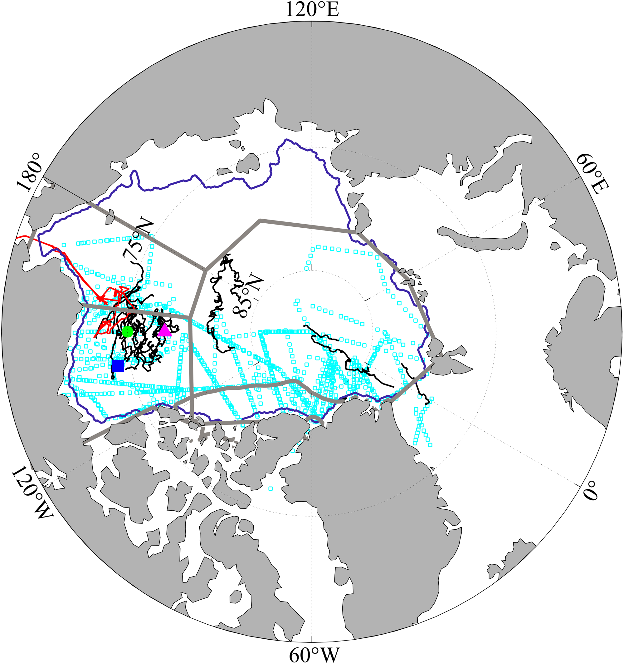
All the locations of in situ observations are applied to the different sea areas according to NSIDC Multisensor Analyzed Sea Ice Extent (MASIE), for example, the Chukchi Sea, the Beaufort Sea, the Central Arctic and NOCAA. They are plotted in Figure 1 in this study.
Locations for all the observations used in this study. The blue square, green circle and magenta triangle represent the ULS locations of BGEP_A, BGEP_B, BGEP_D, respectively. The black lines represent the IMB buoy routes. The cyan squares are the locations of Operation IceBridge Quicklook. The red line shows the track of Sea State Observation. The SIV is calculated over the area enclosed by the purple curve. The gray lines represent the boundary of different sea areas based on NSIDC MASIE, (a) the Chukchi sea, (b) the Central Arctic, (c) the Beaufort Sea and (d) north of the CAA.
3. Methods for evaluation
The TOPAZ4 SIT (referred to as TP4 in the equations for simplicity) is evaluated based on the datasets listed in Section 2 (collectively referred to as Ref in the equations). Compared with in situ observations (except for IMB observations), we select the RMSD, the bias and the correlation coefficient (CC) as evaluation metrics. When comparing with other gridded products, such as PIOMAS, CMST and CS2SMOS, relative difference (RD) is used to quantify the comparison as done in Min and others (Reference Min2019). These metrics can be calculated as follows:
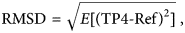

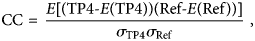
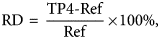
where the operator of E represents the expectation, expressed by the spatial or temporal average. Note that σ TP4 and σ Ref are the standard deviation of SIT in TOPAZ4 and referred datasets.
SIT in IMB and TOPAZ4 have different representations. TOPAZ4 SIT represents effective SIT, which is the average within the model grid, while IMB buoy measures one particular ice floe. Within one model grid (larger than 10 km), the real SIT could change dramatically, thus the SIT from IMB hardly represents the SIT in one model grid. To utilize the IMB data as far as possible, it would be more valuable to compare the SIT temporal variability rather than the exact value. The centred RMSD (CRMSD) that removes the mean of the time series generally meets the demand. Following Mu and others (Reference Mu2018a):

In order to increase visualization, we also plot all statistical metrics in one Taylor Diagram, which requires the following formula to be satisfied (Taylor, Reference Taylor2001):

where σ and σ ref are the standard deviation from the model and the references, respectively. To achieve this, we normalize the standard deviations and the CRMSDs by dividing the standard deviations of the referred observations.
Considering that different maps and resolutions are applied to the gridded products, we only calculate the SIV on the overlapped coverages within the purple curve (Fig. 1). The gridded products, including CS2SMOS, PIOMAS and CMST are linearly interpolated into the mesh grid of TOPAZ4. After that, the SIV is calculated based on the effective SIT (SITeff) and the area of the grid (S grid) as follows:

4. Results
4.1 Spatial distribution of SIT in March and September
Arctic SIV in PIOMAS usually reaches its maximum in April. Since CS2SMOS does not cover the entire April, we choose averaged March SIT instead for intercomparison and evaluation. Averaged SIT in September has also been calculated to gain an insight into the performance of TOPAZ4 during the minimum SIT period. Comparisons of the SIT spatial distribution are performed against PIOMAS, CMST and CS2SMOS in these 2 months. Note that CS2SMOS data are only available in the freezing season. In this study, the overlapped period between TOPAZ4 and CMST is only from 2014 to 2016, while the period used for the other datasets is from 2014 to 2018.
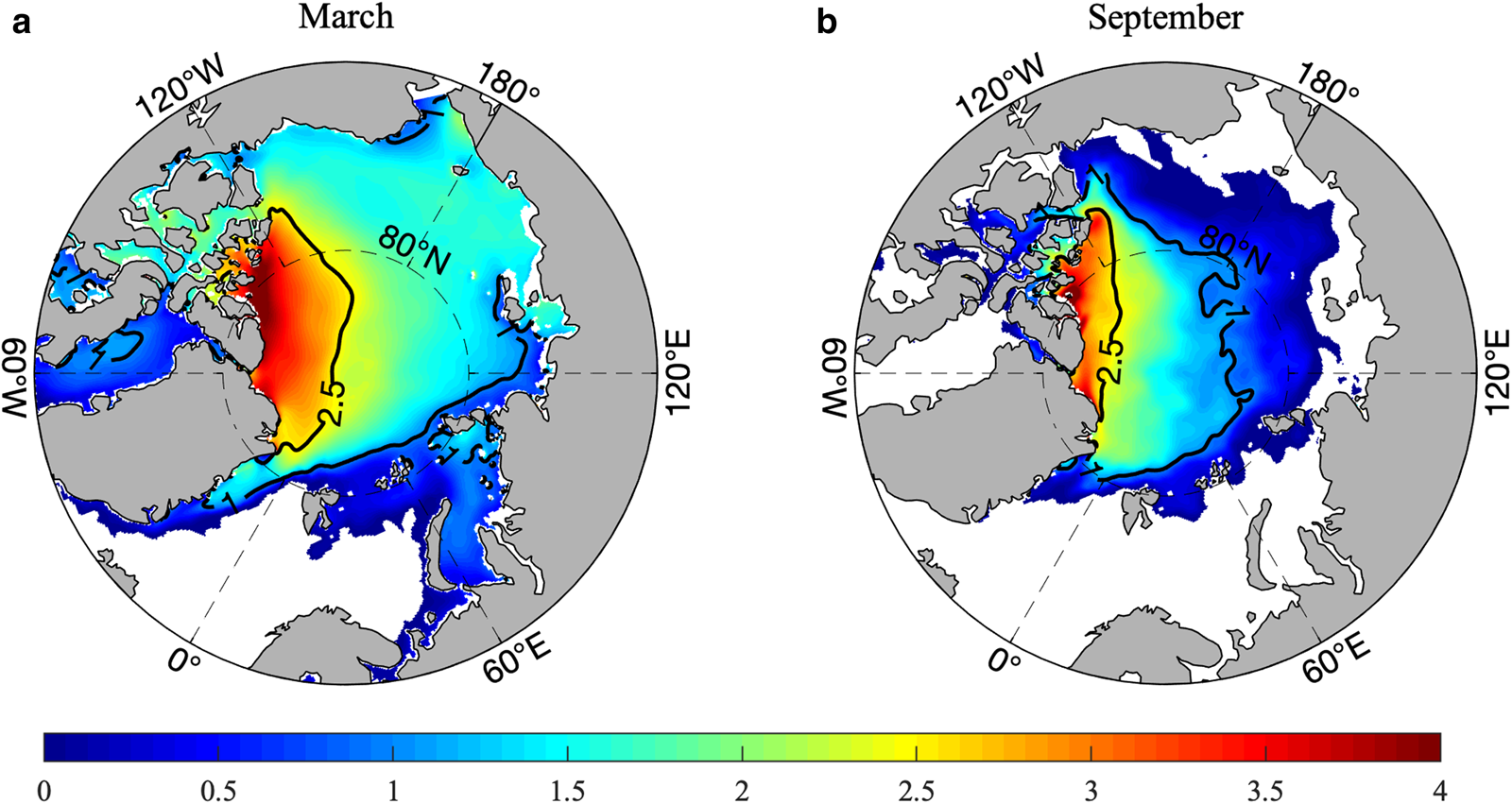
As shown in Figure 2, in March, the TOPAZ4 SIT is found thinner than 1.0 m over the Barents Sea, the Kara Sea, the Laptev Sea and the Baffin Bay. The central Arctic is covered by thick ice of ~2.5 m and the multiyear ice thicker than 4.0 m appears along the northern coast of the CAA. Following the melting season, the sea-ice area in September has reduced ~58% from its area in March. The ice-free area is found along the coast of the Asian Continent.
Five-year (2014–18) averaged SIT in TOPAZ4 for March (a) and September (b). The contours represent 2.5 and 1 m.
The differences and RD between TOPAZ4 and other gridded products are shown in Figures 3, 4, respectively.
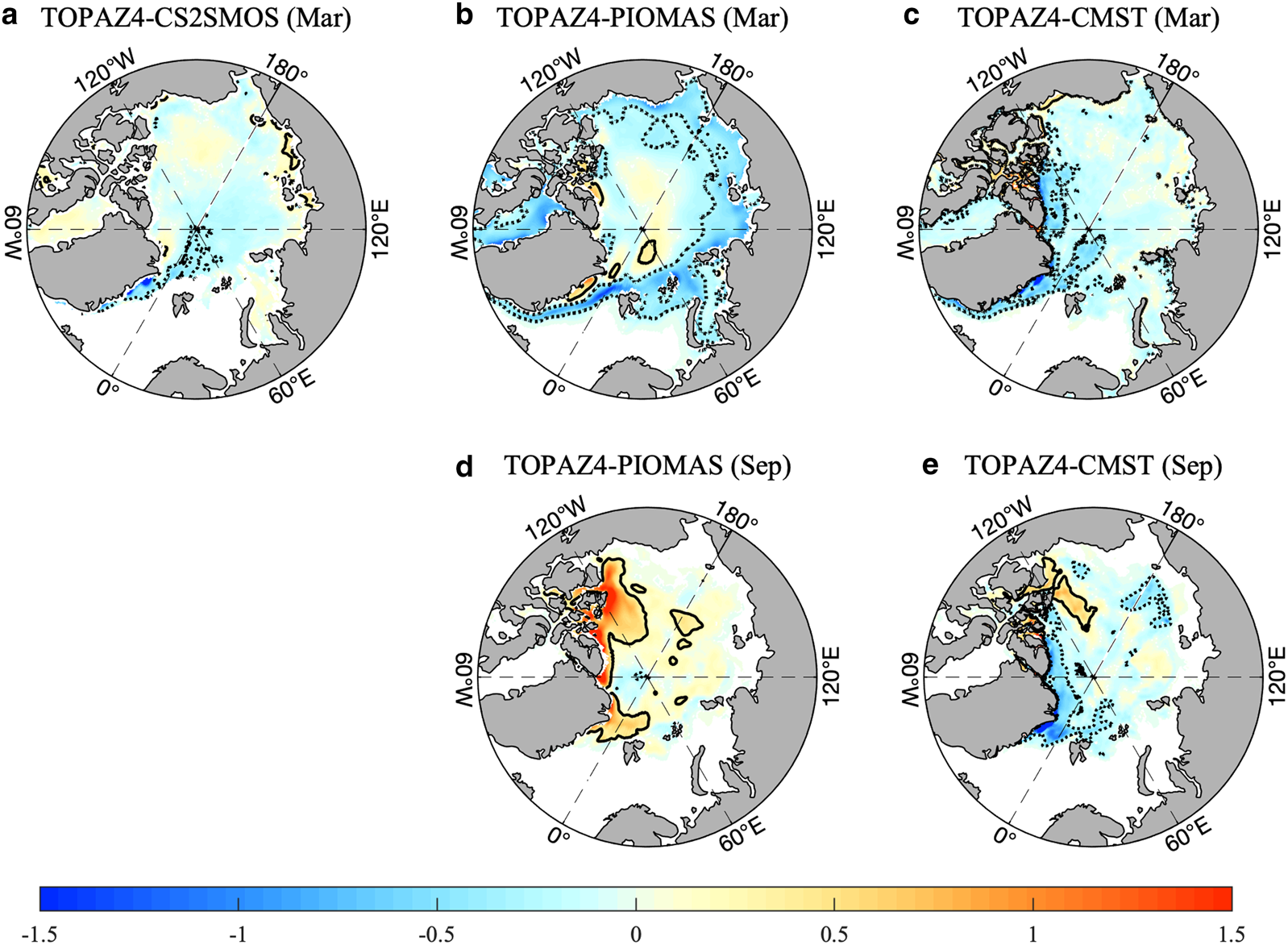
Difference of SIT (in m) between TOPAZ4 and CS2SMOS (a), PIOMAS (b, d), CMST (c, e) in March (top panel) and September (bottom panel). Note that CS2SMOS is not available in September. The period used for CMST is 2014–16, while the period for the other datasets is 2014–18. For every panel, the solid (dashed) lines indicate the 0.3 m (−0.3 m) isolines.
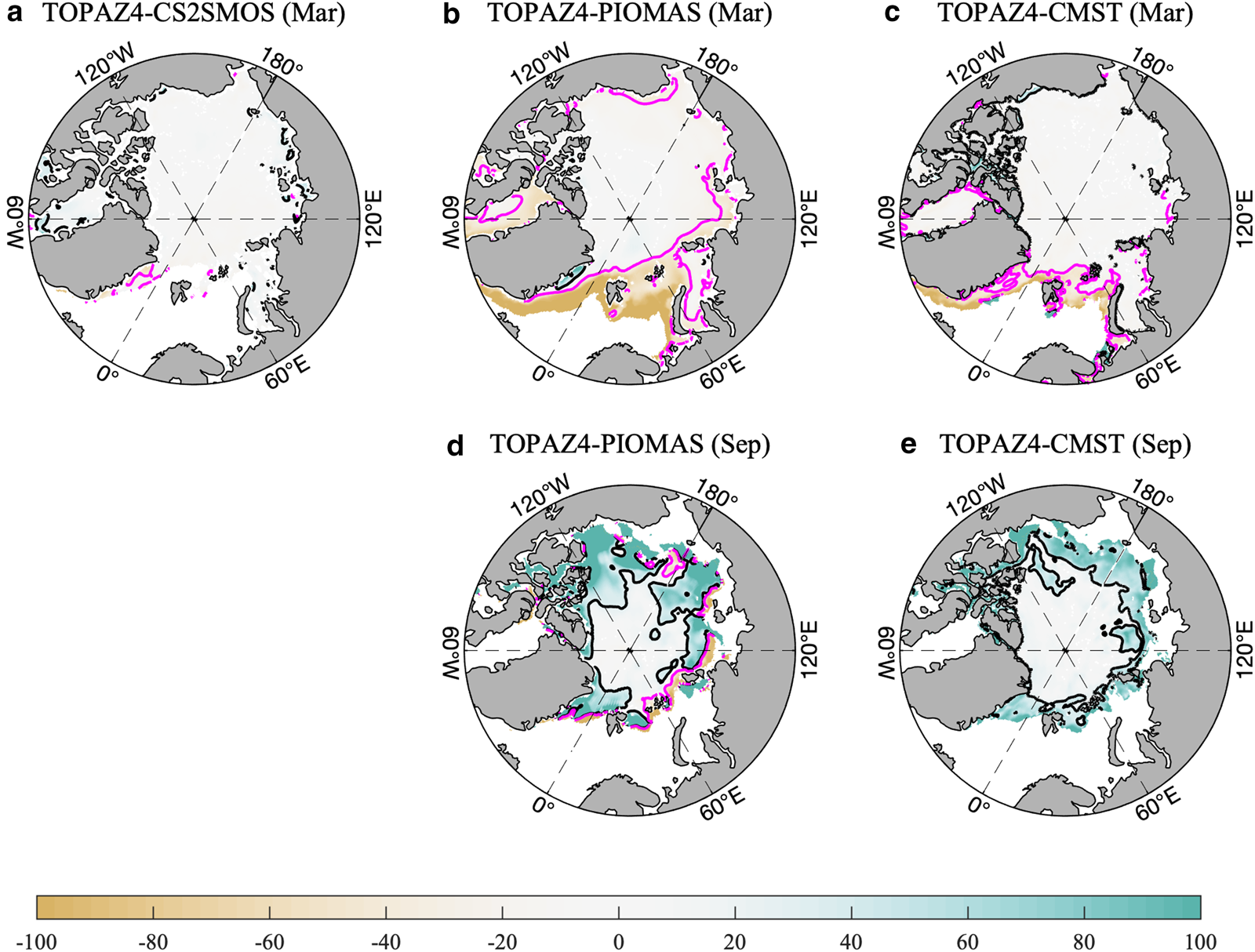
Same as Figure 3, but for the spatial distribution of relative deviation (RD). For every panel, the dark (magenta) lines indicate 30% (−30%) isolines.
In March, due to the influence of assimilating CS2SMOS SIT, TOPAZ4 fits to CS2SMOS very well, with a minimum difference of only 0.04 m and a minimum RMSD of 0.20 m. The major difference is along the eastern coast of the Greenland. By fusing SIT from CryoSat-2 and SMOS, although in different ways, TOPAZ4 and CMST show some agreements. The differences between TOPAZ4 and CMST mainly locate in the American Sector, for example, the NOCAA, the north of Greenland. When compared with PIOMAS, TOPAZ4 also shows reasonable SIT to the NOCAA, though SIT was underestimated in PIOMAS there (Schweiger and others, Reference Schweiger2011; Wang and others, Reference Wang, Key, Kowk and Zhang2016). In September, sea ice in TOPAZ4 is much thicker than in PIOMAS and the difference reaches 1.5 m along the coast of the Parry Islands. The difference between TOPAZ4 and CMST shows a pattern of dipole with thicker ice in the Canada Basin and thinner ice along the northern coast of the Greenland. Statistically, in March, TOPAZ4 reproduces thinner ice than the other three products, with a mean difference of −0.04 m for CS2SMOS, −0.07 m for CMST and −0.25 m for PIOMAS. In September, TOPAZ4 SIT is closer to CMST, with a difference of −0.06 m, but it is 0.21 m thicker than PIOMAS.
The RD shows some spatial and temporal variations. In March, the large RD mainly locates in the Atlantic Sector, especially in the Fram Strait and the Barents Sea (Figs 4b, c), where TOPAZ4 has thicker ice against PIOMAS and CMST. In September, the difference is mainly in the marginal sea-ice zone, such as the Beaufort Sea and the Eurasian Sector, with TOPAZ4 SIT 40% thicker than PIOMAS and CMST (Figs 4d, e).
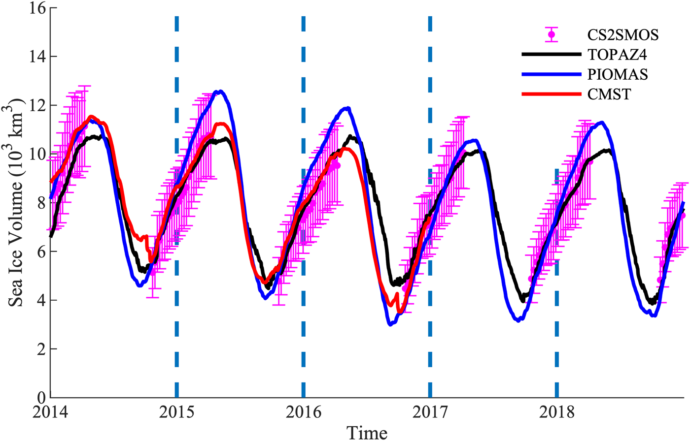
The SIV is also added for intercomparison, given in Figure 5. Considering that different geographical maps are applied to these datasets, for example, TOPAZ4 assumes the Bering Sea is ice-free whereas the CS2SMOS observations suggest the opposite, therefore only the volume within the area enclosed by the purple curve in Figure 1 is calculated using Eqn (7). Similarities and differences of SIV evolution are observed among these four products. Due to the assimilation of SIT from CryoSat-2 and SMOS, despite in different ways, the SIVs in TOPAZ4 and CMST show coherence, especially during the ice growth season. However, differences in the SIV evolutions are clearly presented. For example, SIV in TOPAZ4 fluctuates less than that in PIOMAS as TOPAZ4 reproduces thinner ice in March and thicker ice in September (Figs 3b, d). Besides, TOPAZ4 has a slower ice growth rate during the ice growth season than PIOMAS due to the slower ice growth rate in CS2SOMS. What is more, the melting onset date in TOPAZ4 is slightly later than that in PIOMAS and CMST.
Time series of sea ice volume (in thousands of km3) in TOPAZ4 (black line), PIOMAS (blue line) and CMST (red line). The magenta dot represents CS2SMOS SIV and the error bar is the corresponding uncertainty. The time coverage of these datasets is 2014–18 expect CMST (2014–16).
4.2 Evaluation of SIT against in situ measurements
4.2.1 Comparing with ULS SIT data
The locations of ULS moorings are given in Figure 1, with BGEP_A, BGEP_B and BGEP_D moorings represented by dot, square and triangle, respectively. ULS measures SIT daily from 2014 to 2018. The SIT variations of ULSs and TOPAZ4 (with and without SIT assimilation) are illustrated in Figure 6.
Time series of SIT for BGEP ULS data (blue), TOPAZ4 data (with SIT assimilation, orange; without SIT assimilation, green) at BGEP moorings BGEP_A, BGEP_B, BGEP_D. The shadow areas represent standard deviation for ULS observations.
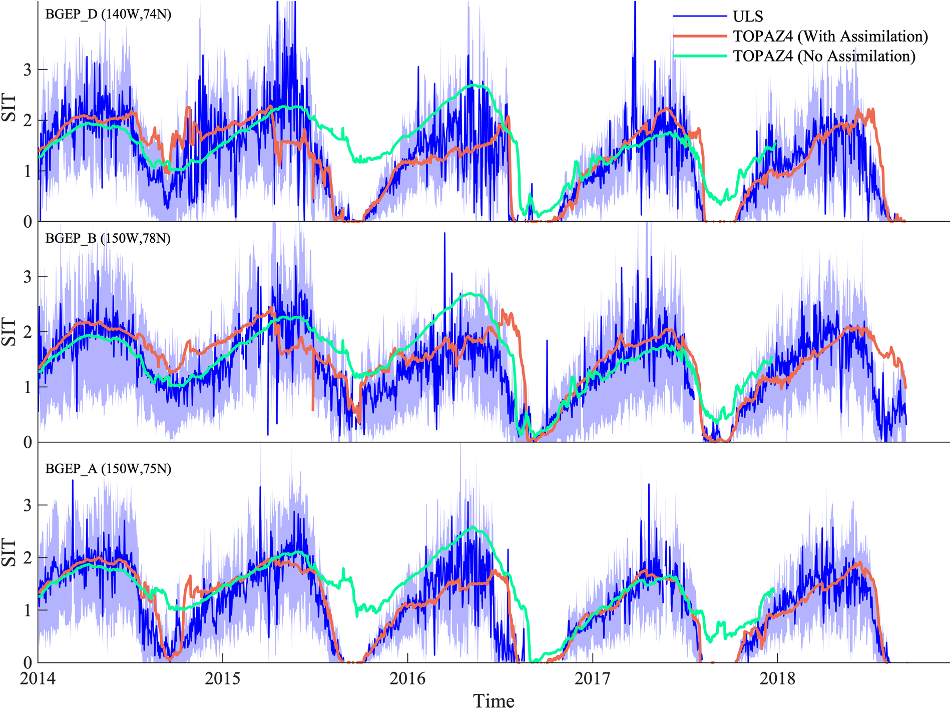
After the SIT assimilation from CS2SMOS, not surprisingly, the mean correlation between TOPAZ4 and ULS SIT is relatively high (0.71). The normalized standard deviation of TOPAZ4 SIT is 0.83 m. TOPAZ4 reproduces the SIT in the freezing season and also shows reasonable results in the melting hiatus. The bias (TOPAZ4 minus ULS) is 0.11 m averaged over the concerned year, with a lower value (−0.06 m) during March and April. Large bias exists in summer (June–July–August) with a mean value of 0.33 m and a mean RMSD of 0.62 m as given in Table 1.
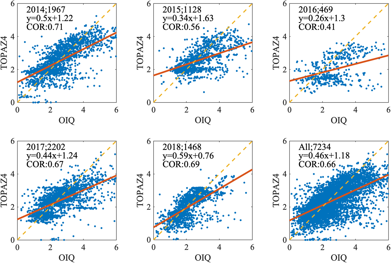
Biases (in m) and RMSDs (in m) for the TOPAZ4 SIT based on ULS measured SIT in the Beaufort Sea in different seasons. ‘All time’ means the temporal-coverage of ULS from 2014 to 2018
Some common deficiencies in TOPAZ4 are presented when compared with these three ULS observations. The melting onset date in TOPAZ4 is significantly later than that in ULS, especially for 2016–18. This shows some coincidences with SIV evolution in Figure 5. The large amplitude and high frequency of SIT variations are generally smoothed in the TOPAZ4 results. This is not surprising, because ULS captures SIT in one particular location, but TOPAZ4 SIT represents the gridcell-averaged value. Large misfits between ULS and TOPAZ4 exist in April 2015. The assimilated CS2SMOS SIT is responsible for the unexpected large reduction of SIT in TOPAZ4 on BGEP_D/B in 2015 (compared to TOPAZ4 without SIT assimilation, Fig. 6, green line). The RMSDs for TOPAZ4 SIT at BGEP_A, BGEP_B and BGEP_D are 0.40, 0.50 and 0.58 m, respectively.
Nevertheless, the benefits of assimilating CS2SMOS SIT are still clear, when comparing to the reanalysis without SIT assimilation, especially in the summer of 2015 and 2017. Assimilating CS2SMOS SIT contributes to a better initial condition at the beginning of melting season and a reasonable SIT change rate. Statistically, when compared to TOPAZ4 without SIT assimilation, the SIT assimilation contributes to an improvement of ~60% in terms of bias, 15% in terms of RMSD and 8% in terms of CC. Our results agree with those from Xie and others (Reference Xie, Counillon and Bertino2018).
4.2.2 Comparing with OIQ SIT data
The Operation IceBridge Quicklook campaigns are conducted in March and April annually, which enable the evaluation of the TOPAZ4 SIT during the freezing season. Observation during each campaign lasts only a few hours but covers a long distance over the western Arctic. The comparisons between IceBridge Quicklook and TOPAZ4 SIT are conducted annually. Further, we evaluate the performance of TOPAZ4 SIT over the Beaufort Sea, the Central Arctic and the Chukchi Sea based on the NSIDC MASIE concept (https://nsidc.org/data/masie/browse_regions). TOPAZ4 SIT is also evaluated for the ridged area, NOCAA (Fig. 1).
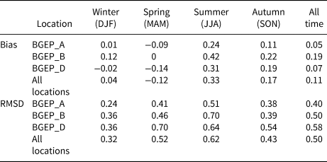
Intuitively, TOPAZ4 simulates thinner ice in March and April, especially along the northern coast of the CAA, in the Beaufort Sea and the Fram Strait (Fig. 7a), where differences over 2 m are observed. The statistical metrics also support this conclusion, for example, TOPAZ4 SIT has a negative bias of −0.21 m, a CC of 0.66 and a RMSD of 0.92 m when compared with the IceBridge Quicklook. Nevertheless, the benefit of assimilating CS2SMOS SIT is obvious. The bias (RMSD) has been reduced to −0.21 m (0.92 m) with a reduction of 81% (34%) when comparing to the results obtained by Xie and others (Reference Xie, Bertino, Counillon, Lisæter and Sakov2017). This quantitatively demonstrates the promising impact of assimilating CS2SMOS into the system. The probability distribution function of the SIT difference between TOPAZ4 and IceBridge Quicklook is shown in Figure 7b. TOPAZ4 performs the best in 2014, with a maximum correlation of 0.71 (Fig. 8) and a bias of −0.13 m.
Difference of SIT between TOPAZ4 and IceBridge Quicklook. (a) Spatial distribution and (b) probability distribution function of the SIT difference..
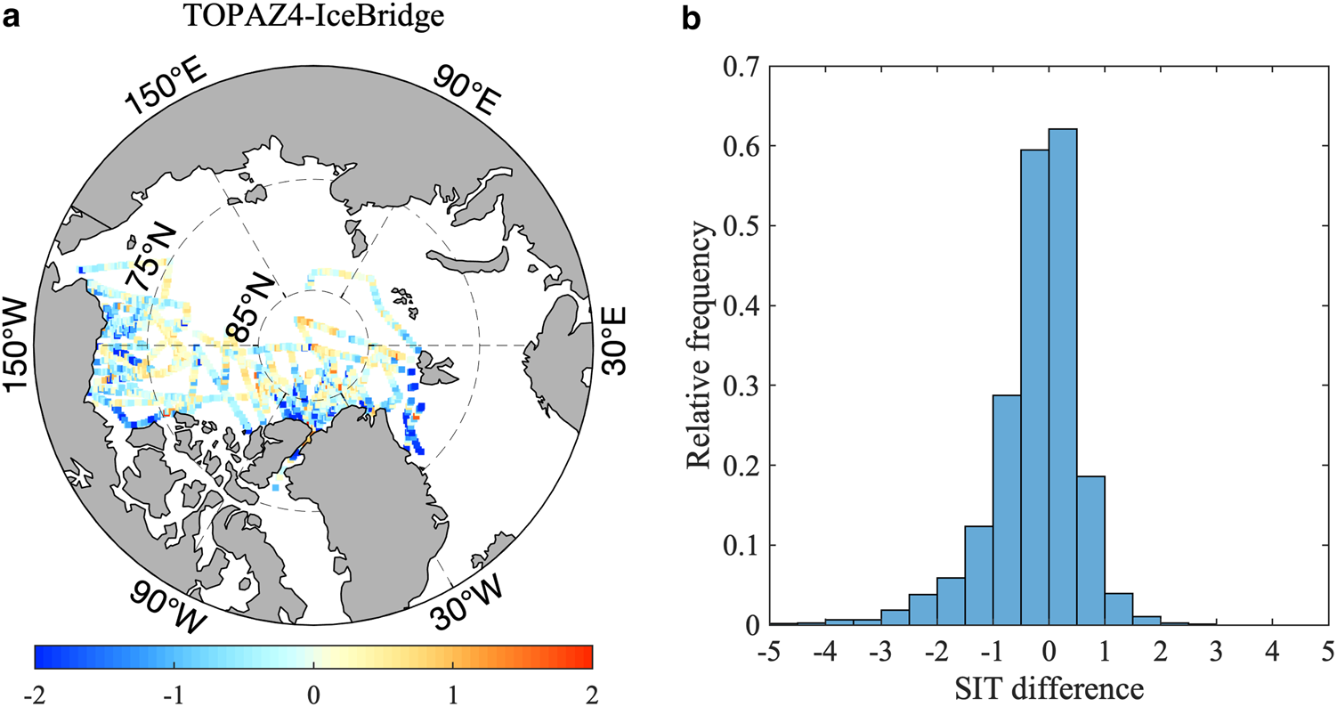
SIT from TOPAZ4 (Y-axis) and gridded averaged SIT from Operation IceBridge Quicklook (X-axis). The years and the numbers of scatters are listed in the top left of each panel. ‘All’ represents all years from 2014 to 2018. Linear equations obtained from univariate linear fitting using SIT from IceBridge Quicklook and TOPAZ4 are given there. They are represented by tangerine lines in respective subplots. The correlations are given below the equations.
We further look into the performance of TOPAZ4 SIT in different sea areas as specified in Figure 1. There were 21 campaigns in the Beaufort Sea, 18 campaigns over the Central Arctic, 4 campaigns over the NOCAA, and 6 campaigns over the Chukchi Sea. Scatter plots in Figure 9 show that TOPAZ4 has the best fit in the Chukchi Sea. The minimum mean bias and the maximum mean CC are, as shown in Table 2, −0.07 m and 0.71, respectively. These results agree somehow with that in Uotila and others (Reference Uotila2019), who found smaller errors (<0.25 m) in TOPAZ4 in the Canada basin, the East Siberian Sea and some parts of the Chukchi Sea, even compared with the errors in other reanalysis products from 2000 to 2012 (see Fig. 5 in Uotila and others (Reference Uotila2019)). The well-performed TOPAZ4 SIT during that period was also benefited from the assimilation of SIC. Consequently, it indicates that both the SIT assimilation and the internal thermodynamics of sea ice may play a part in the Chukchi Sea. For the thicker ice over the NOCAA, TOPAZ4 shows a bias of −0.3 m, indicating TOPAZ4 underestimates the SIT over the ridged ice area.
SIT from TOPAZ4 (Y-axis) and gridded averaged SIT from Operation IceBridge Quicklook (X-axis) in the Beaufort Sea (a), the Central Arctic (b), the Chukchi Sea (c) and north of the Canadian Arctic Archipelago (NOCAA), (d). The sea areas and the numbers of scatters are listed in the top left of each panel. The linear equations obtained from univariate linear fitting using SIT from IceBridge Quicklook and TOPAZ4 are also given there, which are represented by tangerine lines in respective subplots. The correlations are given below the equations.
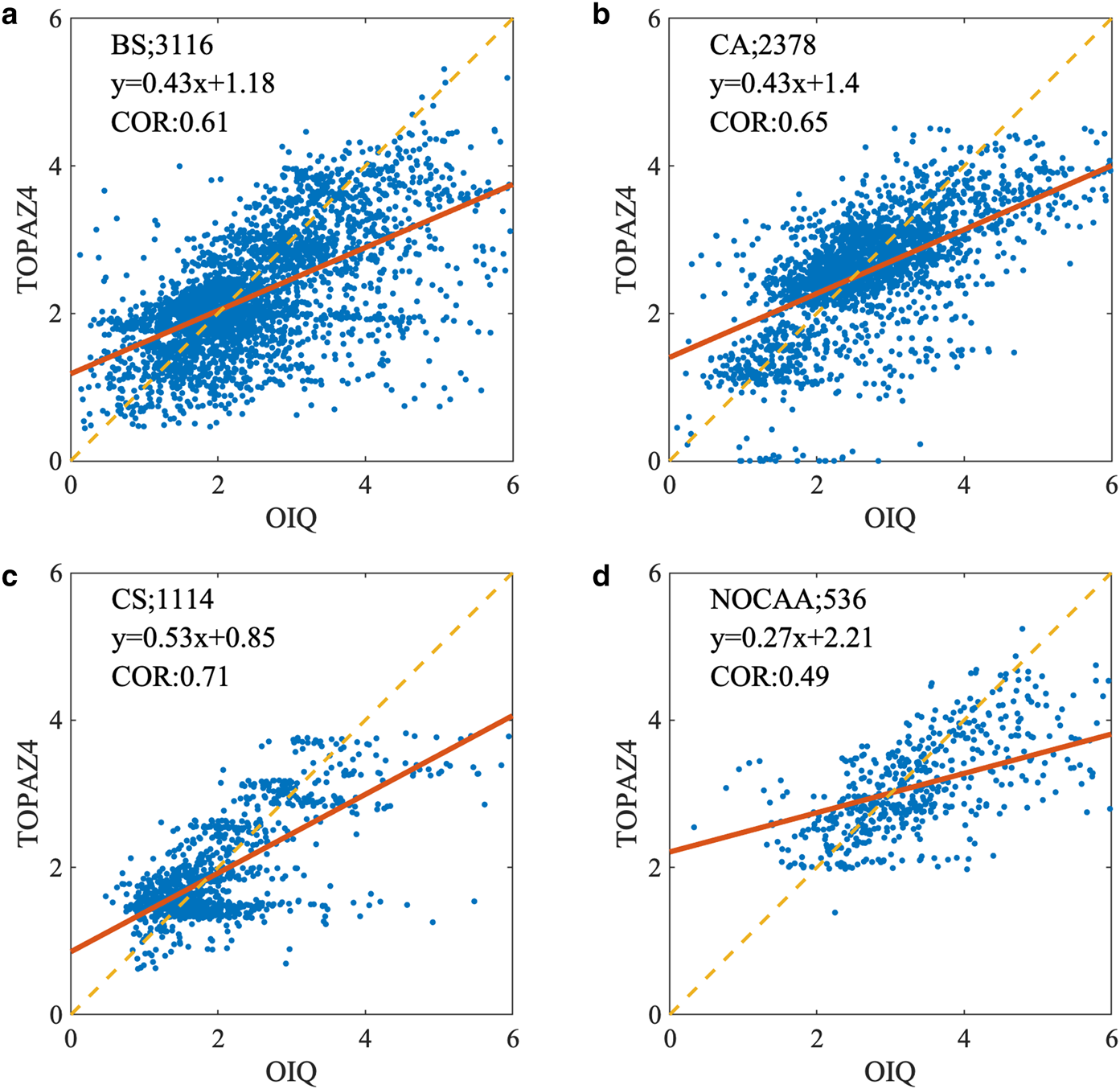
The CC (correlation coefficient), bias (in m) and RMSD (in m) for the TOPAZ4 SIT with respect to IceBridge Quicklook in different years
BS=Beaufort Sea; CA=Central Arctic; CS=Chukchi Sea; NOCAA=north of the Canadian Arctic Archipelago.
Note that the bias represents TOPAZ4 minus IceBridge Quicklook.
All time means the time coverage of IceBridge Quicklook flight campaigns during the freezing season.
4.2.3 Comparing with the IMB buoy SIT
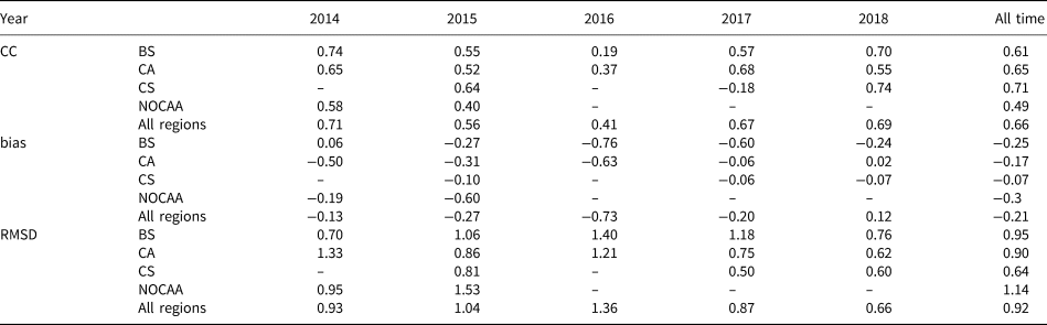
IMB buoys are designed to measure ice growth and ablation. As the equipment is attached to a piece of ice floe, the buoys mainly provide Lagrangian SIT information. Due to the different representations of SITs in TOPAZ4 and IMB buoy, we evaluate TOPAZ4 SIT by comparing the SIT evolution in TOPAZ4 and IMB (see section 3). The trajectory of each buoy is shown in Figure 10a and the performance of TOPAZ4 SIT is diagnosed against each buoy, as shown in Figure 10b. The mean normalized standard deviation is 1.45 m and the CRMSD is 0.48 m. The mean CC between IMB and TOPAZ4 is 0.79.
(a) The trajectories of all available IMB buoys and (b) Taylor diagram for TOPAZ4 SITs with respect to all available IMB buoys data. The radial axis is the Normalized Standard Deviation and the angular axis represents the correlation coefficient. Each circle represents the performance of TOPAZ4 based on one single IMB.
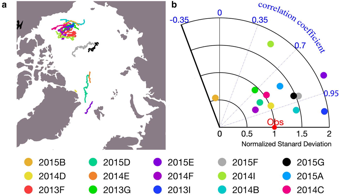
One representative buoy (2013F) was chosen for a case study and its analysis is presented in Figure 11. Overall, TOPAZ4 is able to reproduce the SIT measured by buoy 2013F, with a correlation of 0.69 and a CRMSD of 0.21 m. By analyzing this buoy data, we can gain an insight into the advantage and disadvantage of assimilating CS2SMOS SIT. When CS2SMOS SITs are close to IMB observations, so does the TOPAZ4 SIT (from January 2014 to May 2014). However, when large differences between the two exist, such as an abrupt decline in CS2SMOS ~10 April 2015, assimilating the CS2SMOS SIT value can lead to a large thickness change in TOPAZ4 SIT and causes large misfit of TOPAZ4 SIT with IMB observational SIT. This deteriorates the performance of TOPAZ4 and induces large CRMSD. Even so, TOPAZ4 SIT grows back and it is very close to the IMB buoy observations by 25 June. What is more, a large difference between CS2SMOS and TOPAZ4 can be found from October 2014 to February 2015. This is because that we enlarged the observational error when assimilating CS2SMOS SIT and the SIT difference between CS2SMOS and TOPAZ4 could be reasonable if no more than 0.5 m (Xie and others, Reference Xie, Counillon and Bertino2018). The large difference shown in Figure 11 may be related to the small ensemble spread.
Time series of SIT for IMB buoy (2013F, blue line), TOPAZ4 (tangerine line) and CS2SMOS (black dot). The error bar represents the corresponding uncertainty of CS2SMOS SIT. Date format is YYYYMMDD.
TOPAZ4 reanalysis without SIT assimilation has performed better than that with SIT assimilation when compared to this IMB buoy (2013F). This is due to assimilating the inaccurate CS2SMOS SIT ~10 April 2015. However, this may be avoidable if the inaccurate CS2SMOS could be filtered out. This study helps identify some issues that existed in the current system. Overall, the impact of assimilating CS2SMOS SIT shows the promising effect when considering all IMB buoys’ SIT, as a reduction of 8% in terms of CRMSD is observed.
4.2.4 Comparing with SSO SIT
The Sea State Campaign observes SIT in the Beaufort Sea and Chukchi Sea at a high frequency, which facilitates the performance evaluation for TOPAZ4 during the ice growth season in October 2015. Despite this campaign lasted only for about a month, the comparison with TOPAZ4 will consider the previous results when compared with ULS observation in October.
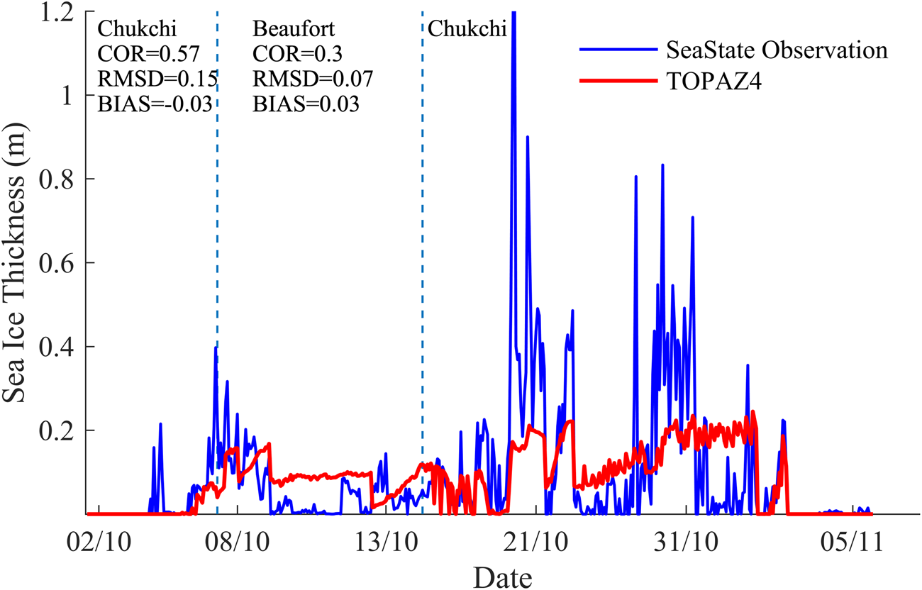
Figure 12 shows the comparison of SIT between TOPAZ4 and SSO along the trajectory of the SeaState Campaign. The descriptive statistics are also shown in Figure 12 for different regions. At ~2 November, the variation and the peak value are well simulated by TOPAZ4. However, TOPAZ4 generally fails to capture the peak and minimal thickness most of the time, for example, ~21 October. During this period, TOPAZ4 SIT has a good correlation with the observed SIT but underestimates SIT for ~1 m. The main reason for this big gap could be that the ship-observed ice does not represent the averaged SIT over a large area. Statistically, TOPAZ4 underestimates SIT by ~0.03 m in the Chukchi Sea, but overestimates SIT by the same amount in the Beaufort Sea. Also, during the same period in ULS observations, the mean bias of TOPAZ4 SIT compared to the ULS observations is 0.21 m. Therefore, we believe that TOPAZ4 reproduce thicker ice in the Beaufort Sea in October.
Time series of SIT along the trajectory of the Sea State Campaign (blue line) and TOPAZ4 SIT (red line) during October 2015.
5. Summary and discussions
A 5-year TOPAZ4 SIT reanalysis product has been generated with the assimilation of SIC from OSISAF and SIT from CS2SMOS. In this study, TOPAZ4 SIT is evaluated with several reference datasets. Despite assimilating SIT reduced the SIT errors by ~28% from 19 March 2014 to 31 March 2015 (Xie and others, Reference Xie, Counillon and Bertino2018), quantified statistics remains to be made to figure out how TOPAZ4 perform based on more observations and over longer period.
Firstly, we compare TOPAZ4 SIT with CS2SMOS, CMST and PIOMAS. In March, TOPAZ4 simulates thinner ice compared with CS2SMOS, PIOMAS and CMST (Figs 3 a–c), and thus shows a smaller SIV in the Arctic Basin (Fig. 5). The RD mainly exists in the Atlantic Sector (Figs 4a–c). In September, the spatial SIT distribution between TOPAZ4 and other reference datasets shows few coincidences. TOPAZ4 SIT is much thicker than PIOMAS along the northern coast of CAA and the northwest of the Greenland, but it is close to CMST (Figs 3d, e). The larger RD mainly exists in the marginal ice area in September, different from that in March (Figs 4d, e), and this difference may result from the different model dynamics.
Secondly, the performance of TOPAZ4 SIT is evaluated against most available in situ observations, including ULS, IceBridge, IMB and SSO. However, the evaluation has been hampered by the sparseness of the observational data. Among all the observations listed above, each observation has its own spatio-temporal coverage. For example, ULS provides SIT information year-round but is only limited to one specific location. On the contrary, IceBridge Quicklook measures SIT over the western Arctic with a long distance, but only for some days in the freezing season. The Sea State and the IMB buoy observations strike a balance between ULS and OIQ, as they provide us data with good spatial coverage (compared with ULS) for a relatively longer period (compared with IceBridge). To make the best use of these in situ observations, we focus on the same period and the same sea area that in situ observations and TOPAZ4 overlap. We evaluate the TOPAZ4 SIT in March–April based on ULS and IceBridge observations, and in October based on SSO and ULS observations. We also assess TOPAZ4 SIT in the Beaufort Sea with data from ULS, OIQ and SSO.
We noticed the consistent variability but different values of bias in TOPAZ4 SIT when comparing to different observational SITs. Comparing with ULS, TOPAZ4 overestimates the mean SIT in the Beaufort Sea by ~0.11 m averaged from 2014 to 2018 (Fig. 6), with the maximum overestimation in summer (Table 1). In October, the overestimation of SIT in the Beaufort Sea is only 0.03 m against SSO (Fig. 12) but 0.21 m against ULS (Fig. 6). Nonetheless, in March and April, TOPAZ4 underestimates SIT in the Beaufort Sea with a bias of −0.25 m comparing with IceBridge Quicklook (Fig. 9a and Table 2) and −0.06 m against ULS (Fig. 6). Actually, TOPAZ4 seems to underestimate SIT in most regions from March to April. The maximum underestimation occurs along the northern coast of CAA based on IceBridge Quicklook, with a bias of −0.3 m and a RMSD of 1.14 m, the bias is relatively smaller over thin ice areas, such as in the Chukchi Sea (−0.07 m). Using the buoy data for evaluation, TOPAZ4 has a good correlation with the IMB SIT, with a mean CC of 0.79. Compared to TOPAZ4 reanalysis without SIT assimilation, the benefit from assimilating CS2SMOS SIT shows an improvement of ~8% in terms of CRMSD.
As shown in Figures 3 4, the differences between different products have potentially large values in some particular regions, including the Fram Strait, the NOCAA and the north of Greenland Island. This implies that a sophisticated sea ice-ocean model, data assimilation scheme and more in situ observations are urgently needed. For example, to improve the simulation along the northern coast of CAA, it is crucial to understand the mechanism of the formation, maintenance and decay of coastal landfast ice (Lemieux and others, Reference Lemieux2015). In order to further reduce the shortcoming of SIT simulation, more realistic physical processes (such as melt pond in summer) in the sea-ice model (Holland and others, Reference Holland, Bailey, Briegleb, Light and Hunke2012) and a more accurate atmospheric forcing are both expected to be developed further. Arctic-wide observational SIT is also needed for assimilation and corroboration, especially during the summer when satellite-derived SIT is not available. In addition, the differences of SIT between TOPAZ4 and CMST/PIOMAS in September are significantly larger than that in March and there are more complicated dynamic conditions (e.g. melting and freezing are purely local, but sea-ice deformations, opening and ridging are far-reaching processes; Rampal and others, Reference Rampal, Weiss, Marsan, Lindsay and Stern2008) in the central Arctic. There is still a long way to reconstruct a consistent time series of Arctic SIT and SIV especially during the melting season.
During the process of generating a reanalysis product, TOPAZ4 assimilates CS2SMOS, which is a merged product from SMOS and CryoSat-2 using an optimal interpolation scheme. Assimilating the merged CS2SMOS is straightforward and easy to implement for operational forecast system, but the uncertainty of the merged product is difficult to quantify. In fact, one can improve the assimilation strategy by assimilating different SIT products. For example, Mu and others (Reference Mu2018b) jointly assimilates SIT and their respective uncertainties from SMOS and CryoSat-2 individually into CMST, and the results presented a better performance of SIT than assimilating CS2SMOS directly. This can be explained by that uncertainties in SMOS and CryoSat-2 SIT are quantified more explicitly than those in CS2SMOS, which has a positive effect of the assimilation performance (Mu and others, Reference Mu2018b). Recently, using a stochastic ensemble Kalman filter semiqualitative (EnKF-SQ) method, Shah and others (Reference Shah, Bertino, Counillon, El Gharamti and Xie2019) showed the advantages of assimilating range-limited thin ice thickness measurement, compared with the results from neglecting the out-of-range value in EnKF. Furthermore, Sallila and others (Reference Sallila, Farrell, McCurry and Rinne2019) showed the CryoSat-2 SIT are reliable between 0.5 and 4 m, so the EnKF-SQ will be promising to seamlessly assimilate these two range-limited SIT observations from CryoSat-2 and SMOS (SIT <0.5 m). It is expected that more precise definitions of the observation errors of satellite-derived SIT are promising to further improve the assimilation performance.
Data availability
The observations used for evaluation, including ULS, IMB, OIQ and SSO, are available from the sources mentioned in the text. The PIOMAS product can be download as mentioned in the corresponding chapter. The CMST SIT products are available at https://doi.org/10.1594/PANGAE A.891475 (Mu and others, Reference Mu2018c). The CS2SMOS SIT product can be downloaded from https://data.seaiceportal.de/data/cs2smos_awi/n/ (Ricker and others, Reference Ricker2017). The TOPAZ4 reanalysis data are available at http://marine.copernicus.eu (Xie and others, Reference Xie, Counillon and Bertino2018).
Acknowledgements
This study is supported by the National Key R&D Program of China (Grant No. 2019YFA0607004), the National Natural Science Foundation of China (No. 41922044, 41941009, 41676185), the Guangdong Basic and Applied Basic Research Foundation (No. 2020B1515020025), and the Fundamental Research Funds for the Central Universities (No. 19lgzd07). This is a contribution to the Year of Polar Prediction (YOPP), a flagship activity of the Polar Prediction Project (PPP), initiated by the World Weather Research Programme (WWRP) of the World Meteorological Organisation (WMO). We acknowledge the WMO WWRP for its role in coordinating this international research activity. We thank two anonymous reviewers and the scientific editor Stephen Jones for their valuable comments to help improve our manuscript.
Author contributions
QY and JX developed the concept of the paper. YX performed the data analysis and interpretation of the results. All co-authors assisted during the writing process and critically discussed the contents.
Conflict of interests
The authors declare that they have no conflict of interest.


 Open access