


Impact Statement
Turbulent Taylor–Couette flow embodies an abundance of rich and enigmatic flow phenomena. We aim to investigate these using the Okinawa Institute of Science and Technology – Taylor–Couette set-up. Here, we outline the salient elements of this set-up, including its unique design, novel instrumentation, robust noise control and streamlined operation. This information may assist experimental studies of a broad range of complex flows.
1. Introduction
Of the multitude of flows that one may study, what makes the Taylor–Couette (TC) flow (Reference CouetteCouette 1888; Reference TaylorTaylor 1923) special? At first glance, the set-up may seem unremarkable: a fluid confined between two concentric cylinders, with both cylinders independently rotating about the central axis. However, a closer examination is instructive. Consider the flow when the outer cylinder remains stationary and the inner cylinder is gradually accelerated. Initially, the flow is purely azimuthal, but as the angular frequency increases, it is suddenly inundated by alternating pairs of counter-rotating vortices known as Taylor vortices (Reference TaylorTaylor 1923). As the angular frequency continues to rise, the Taylor vortices mutate into a sequence of increasingly complex spatio-temporal flow structures. Moreover, when the outer cylinder also rotates, a remarkably intricate flow-phase diagram emerges, filled with a diverse range of ornate flow structures (Reference Andereck, Liu and SwinneyAndereck, Liu & Swinney 1986). Here is a glimpse into this baroque array: wavy vortex flow, twisted vortices, corkscrew patterns, inter-penetrating spirals, turbulent Taylor vortices, spiral turbulence and featureless turbulence. In essence, the seemingly simple TC set-up encompasses a rich assortment of complex flow phenomena.
However, the complexities manifested by TC flow are only half of its allure. A key attribute of the TC set-up is its simplicity. This makes theoretical analysis tractable. Crucially, this essential quality of tractable complexity has yielded many foundational insights into the nature of fluid flow. For example, G.I. Taylor's (Reference TaylorTaylor 1923) pioneering study on how Taylor vortices form substantiated the no-slip boundary condition. It also showed that fluctuating flows can be analysed using the Navier–Stokes equations. The no-slip boundary condition and Navier–Stokes equations now constitute the bedrock for modern analysis techniques of fluid flows. It came to be so in no small part due to Taylor's results.
Since Taylor's seminal work, studies of TC flow have continued to elucidate several fundamental ideas in fluid dynamics. They have also found applications in a wide range of fields, from medicine (Reference Ameer, Barabino, Sasisekharan, Harmon, Cooney and LangerAmeer et al. 1999) to engineering (Reference Van den Berg, Luther, Lathrop and LohseVan den Berg et al. 2005; Reference Fokoua, Gabillet, Aubert and ColinFokoua et al. 2015) to astrophysics (Reference Ji, Burin, Schartman and GoodmanJi et al. 2006; Reference AvilaAvila 2012; Reference Paoletti, van Gils, Dubrulle, Sun, Lohse and LathropPaoletti et al. 2012). A recent theme issue (Reference Hollerbach, Lueptow and SerreHollerbach, Lueptow & Serre 2023; Reference Lueptow, Hollerbach and SerreLueptow, Hollerbach & Serre 2023) commemorating the centennial of Taylor's 1923 paper provides an overview of some of the key advances spurred by this paper. Despite these impressive advances, TC flow still contains a wealth of surprises. Indeed, studies of TC flow continue to uncover unique and puzzling attributes of flow phenomena that defy our understanding. Open problems abound, particularly for turbulent TC flow (Reference Grossmann, Lohse and SunGrossmann, Lohse & Sun 2016). For example, empirical data on torque (or the wall shear stress) (Reference Paoletti and LathropPaoletti & Lathrop 2011; Reference Van Gils, Huisman, Bruggert, Sun and LohseVan Gils et al. 2011b), mean-velocity profile (Reference Huisman, Scharnowski, Cierpka, Kähler, Lohse and SunHuisman et al. 2013b; Reference Ostilla-Mónico, Verzicco, Grossmann and LohseOstilla-Mónico et al. 2016) and energy spectra (Reference Lewis and SwinneyLewis & Swinney 1999; Reference Huisman, Lohse and SunHuisman, Lohse & Sun 2013a) are replete with striking and puzzling features that are distinct from other canonical wall-bounded turbulent flows.
Additionally, as compared with other high-Reynolds-number flow set-ups, a turbulent TC flow set-up furnishes several advantages. Its geometry is simple, it requires a smaller fluid volume and the whole set-up occupies a considerably smaller housing space. Another advantage is the ease of achieving high-Reynolds-number flows. With  $O(10)$ cm radius cylinders, annular gap of $O(1)$ cm and driven by motors of a few kWs power, Reynolds numbers of the order of $10^5$ can be reached without great difficulty. In other set-ups, e.g. a pipe flow experiment, much larger equipment and pumping power would be required to achieve a similar order of magnitude in the Reynolds number. Further, because the flow is confined in a closed system, changing the working fluid is straightforward. Also the working fluid can be easily doped with additives (such as polymers, sediments or bubbles). And, because no external pumping is involved, the additives are not degraded by a pump. (This is a significant concern in studying the effects of polymer doping because polymers can be splintered by pumps.)
On the flip side, a turbulent TC flow set-up also has some disadvantages. Precise control of cylinders rotating at high speeds requires careful design, high-precision machined components and effective vibration control. Further, data acquisition in a rotating set-up poses many challenges. Also, because the system is closed, turbulence continually heats the working fluid. For a steady state, this heat has to be taken out via heat exchangers at the same rate as it is generated. Even seemingly mundane aspects of experiments, such as leakage of the working fluid, can cause significant damage. There is also the need for regular maintenance as rotating parts wear periodically.
We have built a new TC set-up, the Okinawa Institute of Science and Technology – Taylor–Couette set-up (OIST-TC), to study turbulent TC flow. It is housed in the Fluid Mechanics Laboratory at the Okinawa Institute of Science and Technology (OIST), Japan. In embarking on this project, we greatly benefited by studying the design of two well known high-Reynolds-number TC set-ups: (i) the set-up at the University of Maryland (Reference LathropLathrop 1992; Reference Lathrop, Fineberg and SwinneyLathrop, Fineberg & Swinney 1992a), which we refer to as UM-TC; and (ii) the set-up at the University of Twente (Reference van Gils, Bruggert, Lathrop, Sun and Lohsevan Gils et al. 2011a), which is known as the Twente Turbulent Taylor–Couette set-up or  $\text {T}^3\text {C}$. Many of the key advances in our current knowledge of turbulent TC flow can be traced to experiments carried out in these two set-ups. We hope to use OIST-TC to contribute to this endeavour. In this manuscript, we introduce OIST-TC, starting with its design.
2. Design
Taylor–Couette flow is characterized by four governing parameters. Two are geometric: radius ratio,  $\eta _r \equiv R_i/R_o$ and aspect ratio, $\varGamma \equiv L/d$; and two are dynamic: inner-cylinder Reynolds number, ${Re_i} \equiv \varOmega _i R_i d/\nu$ and outer-cylinder Reynolds number, ${Re_o} \equiv \varOmega _o R_o d/\nu$; where indices $(i,o)$ represent the inner and outer cylinder, respectively, $R_{i/o}$ is the radius of a cylinder, $d\equiv R_o-R_i$ is the radial gap, $L$ is the height of the flow region, $\varOmega _{i/o}$ is the angular frequency of a rotating cylinder and $\nu$ is the kinematic viscosity of the fluid. It is also convenient to introduce the bulk Reynolds number ${Re_b}\equiv (\varOmega _i-\varOmega _o)R_md/\nu$, where $R_m=(R_i+R_o)/2$ is the radius of the mid-gap region.
For OIST-TC, the outer cylinder has an inner radius of  $R_o=16.0$ cm and the inner cylinder has an outer radius of $R_i=11.95$ cm. This results in a gap of $d = 4.05$ cm and a radius ratio of $\eta _r = 0.747$. The height of the flow region, which is set by the distance between the top and bottom flanges attached to the outer cylinder, is $L = 60.2$ cm, giving an aspect ratio of $\varGamma = L/d = 14.86$. The values of the geometric parameters, $\eta _r$ and $\varGamma$, are comparable to those of UM-TC and $\text {T}^3\text {C}$, allowing us to benchmark our results against theirs.
We vary the dynamic parameters  ${Re_i}$ and ${Re_o}$ by varying $\varOmega _i$ and $\varOmega _o$, respectively, and by changing the working fluid. With water at 25 $^\circ$C as the working fluid, we can comfortably explore $\varOmega _i \lesssim 160$ rad s $^{-1}$ and $\varOmega _o \lesssim 105$ rad s $^{-1}$, which correspond to ${Re_i}$ and ${Re_o}$ values up to $8.7 \times 10^5$ and $7.6 \times 10^5$, respectively. (The maximum possible values of the inner- and outer-cylinder angular frequencies are, respectively, $\varOmega _i = 210$ rad s $^{-1}$ and $\varOmega _o = 160$ rad s $^{-1}$.)
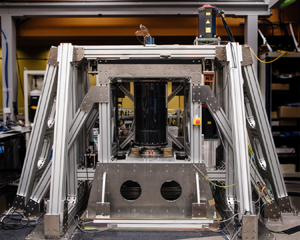
In this section, we describe the primary components of OIST-TC (figure 1).
An annotated photograph of OIST-TC.

2.1 Cylinders
The main section of OIST-TC consists of two concentric, hollow cylinders that can be rotated independently and in either the clockwise or counter-clockwise direction (figure 2a,b). The outer cylinder is made of clear acrylic, allowing full optical access to the flow (see figure 2c and the movies in the Supplementary Material (SM) available at https://doi.org/10.1017/flo.2024.30, for examples of flow visualization). The thickness of this cylinder is 1.5 cm. The inner cylinder is made of aluminium (A5052). Its outer surface is anodized (with black aluminite) to prevent oxidation. Similar to the design in UM-TC and T $^3$C, the inner cylinder is segmented into three sections. This allows us to measure torque in the middle section whilst reducing the end effects. The middle section has a height of $L_m=35.0$ cm, and the top and bottom sections have heights $L_t = L_b =12.3$ cm. The gap between the sections, i.e. between the middle section and the top or bottom section, is 2 mm. The inner volumes of the sections each house at least one temperature sensor, along with a load cell or torque sensor (see § 3). Attendant electronics are housed in the middle section.
Cylinders. (a) A volumetric rendering of the inner and outer cylinders, shaft, and top and bottom flanges. (b) A photograph of the cylinders and their surroundings. (c) Examples of flow visualization at  ${Re_i} = 5550$ (top) and ${Re_i} \approx 1.4 \times 10^5$ (bottom) (see figure S1 in SM for details). Consistent with previous studies (see, e.g. figure 5 in Reference Lathrop, Fineberg and SwinneyLathrop, Fineberg & Swinney 1992b), Taylor vortices are clearly visible at ${Re_i} = 5550$ but are difficult to discern at ${Re_i} \approx 1.4 \times 10^5$.

The cylinders are held in place by a stainless steel (SUS 304) shaft. The shaft is hollow and has slotted holes for passing cables inside the shaft. (These cables leave the shaft via a rotary slip ring at the top; figure 1.) The shaft has sections of different diameter so as to facilitate assembly and to hold the inner-cylinder sections and outer-cylinder end flanges in their correct locations (figure 5a).
Each section of the inner cylinder has two end lids. They are made of anodized aluminium. The lids are mounted to the shaft using NTN6012 ball bearings. They provide a low-friction coupling and can withstand radial loads. The bearings, along with shaft spacing rings and the different shaft sections, correctly position the inner cylinders along the shaft. Each inner-cylinder section rotates with the shaft, coupled to it by a torque sensor or a load cell located inside the section.
The outer cylinder is mounted on two end flanges. They provide structural support to the outer cylinder and also act as heat exchangers for the flow (see § 2.2). Additionally, the top flange contains two acrylic windows, 180 $^\circ$ apart, in order to allow optical access from above the set-up. The cylinder is rotated via the bottom flange. The flanges are mounted on the shaft using angular contact, low-friction ball bearings (NSK 50BAR10ETYNDBLP4A for the bottom flange and NTN 7010CTYNP4 for the top flange). Additional details of the flanges are discussed in § 2.2.
An important consideration for the experiments is to minimize the sources of external vibrations on the flow. There are two main sources: vibrations from driving motors (which we discuss in § 2.3) and vibrations from rotating cylinders. To minimize the vibrations from the cylinders, both cylinders were machined. In addition, we perform static balancing of the inner cylinder (with all the instruments attached) and outer cylinder (with both flanges attached) separately to further minimize any remaining azimuthal imbalance.
Thus far, we have used air and water as the working fluids. When water is used as the working fluid, tiny air bubbles can form and stay attached to the surface of the cylinders even when they are rotating. To solve this problem, we degas the water using a Deo Vac MDG-20S071VLP-T1 system. This eliminates the bubbles. Another potential problem is water leaks. This can be internal, where the water seeps inside the inner cylinder. It can not only affect measurements but also damage the instruments housed within the cylinder. The leak can also be external, seeping out of the set-up, wetting the surroundings. To prevent water leakage, we fitted the inner-cylinder lids and the bottom and top flanges with marine-grade radial seals (Trelleborg TRE000650). We have run OIST-TC with these seals for over 100 hours of operating time, and they have yet to fail or show any visible signs of wear. As a safety precaution, we installed resistive leakage detection sensors inside the three sections of the inner cylinder. They are mounted flush with the bottom lids of each section.
2.2 Heat exchangers
The temperature of the working fluid is controlled via the top and bottom flanges, which act as heat exchangers. The surface of the flange in direct contact with the working fluid is made of heat-conducting brass. Within each flange reside cooling channels through which the coolant (water) is circulated. The temperature of the coolant is controlled by an external chiller (HRSH150-W-20-K). The outer layer of the flange is made of stainless steel (SUS 304) and provides structural rigidity.
Similar to the  $\text {T}^3\text {C}$ design, the coolant is fed to the cooling channels of the bottom flange by a standard rotary union (Deublin 2620-430-252). This rotary union is mounted to the base of a stainless steel (SUS 304) cup constructed with channels to guide the coolant to the bottom flange. (This cup also serves as the mounting point for the bottom driving gear and main bottom bearings.)
For the cooling in the top flange, our design is different from that of  $\text {T}^3\text {C}$. In $\text {T}^3\text {C}$, the coolant is pumped from the bottom flange to the top flange and then returned to the bottom flange through pipes attached to the exterior the outer cylinder. (These pipes rotate with the outer cylinder.) We pursue a different approach: (i) to avoid obstructions around the outer cylinder in order to maintain continuous optical access for flow measurement; and (ii) to control the temperature of the top and bottom flanges independently (this can be used, e.g. to impose a vertical temperature gradient onto the TC flow).
Unlike at the bottom of the cylinder assembly, where the base rotates with the outer-cylinder flanges and allows a simple rotary union to couple water into the cooling channels, at the top flange the uppermost elements prevent such an arrangement. Specifically, as the shaft passes through the top flange and then meets the driving pulley and belt, any rotor/stator combination for the outer cylinder's cooling circuits must also allow for the rotation of the main shaft. In order to accomplish this coupling, we devised the system shown in figure 3(a).
Temperature control. (a) A volumetric rendering of the new design for the top flange's coolant feeding system. (b) Zoomed-in view of the contact between the graphite rings and ceramic plate. (c) Temperature time series from three temperature sensors at three axial locations (top, middle and bottom) in the middle section of the inner cylinder. The working fluid is water. The data correspond to  ${Re_i} = 2.6 \times 10^5$ and ${Re_o} = 0$. Lines of different colours correspond to the three locations. The thin lines represent the data from the sensor, sampled every second. The thick lines represent the corresponding moving average over one minute. The slope of the linear trend line for each sensor is <0.01 $^\circ$C h $^{-1}$, signalling that the temperature is approximately constant in time. Also note that there is no discernible temperature difference between the three locations, signalling that the temperature is uniform in space.

The coolant enters and exits the TC assembly through an annular cooling stator. It is placed coaxially with the shaft and its hollow core facilitates the placement of bearings to allow the shaft's rotation. Underneath the cooling stator is a ceramic plate that is fastened to the top flange, rotating with the outer cylinder. We use the concept of a mechanical seal, akin to those found in centrifugal pumps, to couple the rotating plate with the stator. The bottom surface of the cooling stator has three grooves fitted with graphite rings. Correspondingly, the top surface of the ceramic plate has three matching rails; the contact between the graphite rings and ceramic rails provides the necessary sealing for the coolant whilst also being a low-friction contact point. The coolant flows between the cooling stator and the ceramic plate through the channels formed by this contact (figure 3b). Finally, these channels are connected with the cooling channels of the top flange. With the heat exchangers for the top and bottom flanges engaged, we can keep the working fluid at a constant temperature (<0.01  $^\circ$C h $^{-1}$; see figure 3c).
2.3 Frames
The cylinders are structurally supported by the main frame (figure 1). A key design consideration is to minimize the vibrations from the driving motors to the TC flow. To that end, we use a split-frame design wherein the motors are hosted on a motor frame that is structurally separate from the main frame (figure 1; figure S2 in SM). Some vibration is still communicated, mainly through the timing belts that convey the motors’ torques to the cylinders. Another consideration is that the frames are bolted onto the concrete floor of the laboratory and thus can communicate vibrations. It is, however, of negligible magnitude as the laboratory is located at the ground level of a large building. In addition to its function as a vibration isolator, the split-frame design also provides electrical isolation between the sensors and the motors, which aids in preventing ground loops.
The frames are constructed from extruded aluminium profiles. At several locations, we have reinforced the structure using aluminium plates. These increase the stiffness of the frames and thus increase their natural frequency. Having the natural frequency of the frames be much larger than the loading frequency (the rotational frequency from the motors) ensures that the frames do not have large-amplitude vibration.
The cylinders are installed into the main frame sandwiched between two horizontal plates: a lower mounting plate and an upper mounting plate. Both plates are made of aluminium and are 30 mm thick. The lower mounting plate provides a  $120$ mm diameter enclosure into which, encased by NSK 120BAR10STYNDBLPAA bearings, the shaft is lowered, supporting the weight of the complete cylinder assembly. The upper end of the shaft is supported by the cooling stator, which is mounted to the upper mounting plate. This plate is attached to the top of the main frame using a $U$-shaped bracket and allows for linear translations in the horizontal plane to align the cylinders with the vertical axis.
We monitor the vibration of the main frame using a Schenck SmartBalancer system with two vibration sensors that are placed on the two mounting plates. The maximum value of the root mean square (r.m.s.) of the vibrational velocity time series is approximately  $0.4$ mm s $^{-1}$, which, according to the ISO 20816-3:2022 specification, falls under Zone A (newly commissioned machines) (ISO 2022).
2.4 Motors
The inner and outer cylinders are driven independently by a pair of AC servo motors (Fanuc  $\alpha$iF 30/4000), the top motor driving the inner cylinder and the bottom motor, the outer cylinder. The motors are controlled by a Fanuc 35i-B controller. We use it to set the rotational speed and direction of each motor (which, in turn, sets these parameters for the corresponding cylinder). For the rotational speed, we can specify its time evolution, e.g. linearly increasing with time from rest to a specified value. The controller also provides an emergency stop function for bringing the motors immediately to a halt. We measure the rotational speeds of the two cylinders via rotary encoders (figure 1) connected to a real-time system, which will be discussed further in § 3.5.
The torque from each motor is transmitted to the respective cylinder by a pair of gears (one attached to the cylinder and one to the motor) and a timing belt that connects the gears. The gear reduction can be varied by changing one or both of the motor and cylinder gears. A series of idlers are placed between the main gears. We tension the belts by adjusting the positions of the idlers so as to minimize the vibrations in the frame and the r.m.s. values of the torque and rotational speeds of the cylinders.
3. Instrumentation
3.1 Velocity
We measure the velocity time series of the TC flow using two techniques: laser Doppler velocimetry (LDV) with water as the working fluid and constant temperature anemometry (CTA) with air as the working fluid. The technique of LDV is standard (see, e.g. Reference Huisman, Van Gils and SunHuisman, Van Gils & Sun 2012) and we do not discuss it here. Conducting CTA measurements in a TC flow is challenging for the cases when the outer cylinder rotates. This is because introducing a CTA probe (commonly known as a hot-wire probe) into the flow is non-trivial. This cannot be done through an end flange because the outer cylinder is mounted on (and rotates with) the end flanges. We introduce the hot-wire probe (Dantec 55P14) through the inner cylinder, mounting the probe in the  $2$ mm gap between the middle section and the top section (figure 4). A radial slot was milled in the bottom lid of the top section, with the same diameter as the probe support ( $4$ mm; Dantec 55H20). This allows the probe to tightly fit into the lid and be flush with the surface. The probe was then securely held in place via a thin stainless steel plate bolted onto the lid. A hole was drilled through this lid to pass the probe support cable into the top section and then redirected through the shaft to the electrical slip ring.
A volumetric rendering of the CTA probe mounted on the inner cylinder in the flying hot-wire configuration. The probe causes minimal disturbance on the azimuthal flow as its blockage area is only  $\approx$0.1 % of the cross-sectional flow area (in the axial–radial plane).

The probe rotates with the inner cylinder, sweeping through the mid-gap region of the TC flow. The configuration is known as a ‘flying hot-wire’ set-up. Significantly, this configuration allows us to conduct measurements when either or both cylinders rotate. To our knowledge, this is the first TC set-up to implement a flying hot-wire.
The signal from the probe needs to be conveyed out of the rotating inner cylinder. To that end, we pass the probe support cable through the shaft and connect its BNC end to a custom-made slip ring (Barlin Times THR-008 T-2202-02S) with  $50\varOmega$ paths to avoid any impedance mismatch. From the slip ring, a $4$ m
$4$ m  $50\varOmega$ coaxial cable was connected to the Dantec Streamline Pro CTA system. We built an in-house LabVIEW application to measure the voltage signal output by the CTA system. The voltage signal was acquired using a NI-6361 (16bit) USB data acquisition device. The overheat ratio was set to $0.8$ to improve the frequency response, which results in an overheat temperature of $\sim$226 $^\circ$C (the ambient temperature was 24 $^\circ$C) (Reference JørgensenJørgensen 2005). A square-wave test was performed, and the CTA settings were optimized to maximize the frequency response ( $\sim$60 kHz for a 10 m s $^{-1}$ flow) while avoiding bridge oscillations (slight overdamped response; see Reference Samie, Hutchins and MarusicSamie, Hutchins & Marusic 2018). The signal was acquired at $60$ kHz with a $30$ kHz low-pass filter to avoid aliasing.
We calibrate the probe using a Dantec StreamLine Pro Automatic calibrator. This system generates a controllable jet flow for CTA calibration. We place the probe near the jet's exit (in the jet's core) and calibrate it with velocities ranging from  $0.5$ to 20 m s $^{-1}$. Prior to the calibration, as part of the initial system configuration, we measure the ambient temperature in order to set the decade resistance for the desired CTA operating temperature. This ambient temperature can be different from the flow temperature during calibration. To account for the effect of this temperature difference, we correct the probe's voltage signal by using Bearman's method (Reference BearmanBearman 1969; Reference JørgensenJørgensen 2005). (We follow the same procedure during measurements in the OIST-TC.) Thereafter, we apply a fourth-order polynomial fit to the calibration data to convert the corrected voltage signal to a velocity signal.
3.2 Torque
We measure the torques on the three sections of the inner cylinder. Each section couples to the shaft with either a load cell or a torque sensor (figure 5a). In the top and bottom sections, due to limited space, we use parallelogram load cells (Futek LSM300). These sensors have a wide range of full scale ( $\sim$10–900 N) and a high precision ( $0.02$ % of full scale). The middle section is fitted with a hollow-flange-reaction torque sensor (SensorData T123). However, it can also be configured with a load cell. For the torque sensor, depending on the application, we select a $5.7$ N.m, $22.6$ N.m or $56.5$ N.m capacity sensor. This sensor is fastened in place via two internal flanges (made with SUS 304), one that attaches the sensor to the middle section, and the other connecting the sensor to the shaft (which is keyed to the shaft to avoid slippage); figure 5(b). Although this sensor has a lower accuracy ( $0.1$ % of full scale) than the load cells, the cylindrical construction allows for a better physical connection and reduces observed hysteresis.
Sensors. (a) Locations of sensors for measuring torque and temperature. (b) A volumetric rendering of the torque sensor and its coupling flanges. Also depicted are the temperature and torque PCBs. All these items are located in the middle section of the inner cylinder.

We calibrate the torque measurement system in situ. We apply torque on the inner cylinder via a horizontal belt which is wrapped around the middle section (with either a load cell or the torque sensor inside). The belt passes over a low-friction pulley and a range of weights (with certified calibration) are hung vertically from it.
3.3 Temperature
We measure the temperature across the height of the inner cylinder using five platinum resistance temperature detectors (RTDs). Their sensors are placed flush with the inside surface of the inner cylinder; we use three RTDs in the middle section and one each in the top and bottom sections (figure 5a).
A ratiometric measurement of the resistance is made in order to improve accuracy and avoid a requirement for a high-precision constant current source. We calibrate the RTD sensors to remove systematic variability due to manufacturing variations by using a heat bath (Julabo Corio CP-200F). During the calibration process, temperatures are sampled between 15  $^\circ$C and 45 $^\circ$C, with each point taken after stability (within $\pm 0.03\,^\circ {\rm C}$) is achieved by the heat bath. The results of this calibration are stored as a look-up table (LUT), with linear interpolation between points, to correct measurements made during experiments.
3.4 Analogue to digital conversion (ADC)
The torque sensor and load cells produce analogue voltages as their output signals. These signals convey changes in torque as small changes in voltage, and even after amplification they remain sensitive to electrical noise. Both passing an analogue signal though the slip ring and the presence of nearby AC servo motors can incur considerable noise, adding significant uncertainty to measurements. Converting from analogue to digital signals immediately within the cylinders, on the other hand, confers significant noise reduction.
We custom designed two printed circuit boards (PCBs) for digitizing the analogue signals. Both PCBs are located inside the middle section of the inner cylinder (figure 5). We use one PCB to digitize amplified signals from load cells and the torque sensor (cf. § 3.2). The core functionality of the board is provided by an AD7608 chip ( $18$-bit bipolar simultaneous sampling ADC) with an onboard analogue antialiasing filter. Communication with the PCB is carried out using serial peripheral interface (SPI), for which the torque signal is transmitted as a series of high-frequency digital pulses. This means that small changes in voltage level are irrelevant to the communicated value, and the acceptable level of noise is greater than $1$ V. From our tests, the peak-to-peak noise level went from $400$ mV (analogue signal) to $2$ mV (digital signal) when the servo motors were energized but with no rotation, a noise reduction of $200$ times.
We use the second PCB for the signal from the RTDs (cf. § 3.3). We choose to digitize RTD signals inside the cylinder rather than using externally digitized thermocouples for the same reason as described above for the torque measurements; namely, noise immunity at the slip ring and with regards to the servomotors. The second PCB's core functionality is provided by an LTC2983 chip. Up to five sensors can be connected to the board, each using a  $4$-wire Kelvin sensing configuration, and the ratiometric measurements of their resistances provide the temperature to an external system via SPI. The PCB uses a total of $8$ cables, reducing the required channel count for the slip ring when compared with five $2$-wire thermocouples.
3.5 Rotation speed
We measure the rotation speeds for each cylinder using a pair of Omron E6C3-CWZ5GH rotary encoders with  $3600$ pulses per revolution (figure 1). These sensors are connected to a NI-9361 counter module in the CompactRIO (see § 4). The counter module and the CompactRIO provide convenient tooling to convert sample-clocked frequency measurements to rotation speeds. The combination of a high-resolution rotary encoder ( $3600$ pulses/revolution) with a high-frequency counter module ( $100$ MHz) internal counter clock and a sampling rate of $1$ kHz allow a measurement error of $0.0012$ rpm at $100$ rpm.
4. Operation, automation and data storage
We control the OIST-TC system using GUI-based applications written using LabVIEW. Low-level communication with hardware is managed by a real-time application running on a CompactRIO-9045 device, together with the embedded field-programmable gate array board. Measurement results are packaged together with appropriate metadata by the CompactRIO system before being transferred to networked computers on request, where desktop LabVIEW applications are used to send instructions to the CompactRIO and display ongoing or historical results. The CompactRIO system also logs rotation speeds and periods to a local database, together with the motor controller parameters (Fanuc PLC parameters) relating to the motor feedback loops.
To accomplish the necessary experimental needs of the OIST-TC, we developed libraries for all hardware components as well as for the storage of measurements. These allow us to easily and quickly develop new applications tailored to the needs of our experiments while minimizing the potential introduction of bugs or safety issues. These libraries are automatically compiled, version controlled, and delivered as packed project libraries (PPL) to the real-time system and the laboratory's workstation. The PPL compilation system uses Docker containers managed by a local GoCD continuous integration/continuous delivery system (Reference ButcherButcher 2022), together with a webhook proxying system hosted by OIST's Scientific Computing and Data Analysis section.
Data and relevant parameters from experiments are stored using the NI Technical Data Management Streaming (TDMS) format via a ‘Measurement Results’ PPL. In addition to all the sensors’ data (raw and processed), examples of the stored parameters include local sea level atmospheric pressure (fetched via an API at the time the data are captured), working fluid, experiment type and sensor information (including location, model, range and calibration, if appropriate).
Data analysis and the displaying of results are then performed using MATLAB, for which we developed a system of automated post-processing scripts. The removal of user intervention guarantees consistency of results when processing the data. We use the information inside the TDMS files for this purpose. The results are then stored using MATLAB's .mat format, together with all the TDMS properties, allowing us to backtrack and revisit older processed datasets quickly.
5. Results
5.1 Mean-velocity profile
We measured the mean-velocity profile across the radial gap and in the mid-axial plane using LDV, with water as the working fluid. For the LDV measurements, we used a Dantec FiberFlow  $5$ beam system with a $240$ mm front lens, together with the $488$ nm (blue) and $514.5$ nm (green) wavelengths of a Coherent INNOVA 70C laser. For seeding particles, we used silver-coated silica spheres (mean particle size of $7.5$
$7.5$  $\mathrm {\mu }$m – Potters Conduct-O-Fil SG02S40). We processed the LDV time series data using ray tracing to correct for the curvature effects from the outer cylinder (Reference Huisman, Van Gils and SunHuisman et al. 2012). After applying the correction, we extract the time series of the azimuthal velocity component, $u_\theta (r, t)$. Its time average yields the mean-velocity profile, $U_\theta (r)$.
In figure 6, we show an example of the dimensionless  $U_\theta (r)$ profile. For comparison, we also show a corresponding profile from an experiment (Reference Huisman, Scharnowski, Cierpka, Kähler, Lohse and SunHuisman et al. 2013b) in $\text {T}^3\text {C}$ for comparable values of Reynolds number and radius ratio as the OIST-TC. We note that the two profiles are in excellent accord.
Dimensionless mean-velocity profile across the radial gap. We show LDV data from OIST-TC ( ${Re_i} \approx 84\,000$, $\eta _r = 0.747$) and, for reference, particle image velocimetry (PIV) data from $\text {T}^3\text {C}$ (Reference Huisman, Scharnowski, Cierpka, Kähler, Lohse and SunHuisman et al. 2013b) ( ${Re_i} \approx 100\,000$, $\eta _r = 0.716$). For both cases, ${Re_o} = 0$. We normalize $U_\theta (r)$ using $U_i \equiv U_{\theta }(r = R_i)=\varOmega _iR_i$. We normalize the gap as $\tilde {r}=(r-R_i)/(R_o-R_i)$. The spatial resolution of the LDV profile is $0.285$ mm and the PIV profile is $0.15$ mm. For ease of comparing the two profiles, we plot the data points undersampled at a resolution $\Delta \tilde {r} \approx 0.015$. The LDV profile starts at $\tilde {r} \approx 0.02$; reflections from the inner-cylinder wall make it difficult to measure the velocity at small $\tilde {r}$ (see, e.g. Reference van Gils, Huisman, Grossmann, Sun and Lohsevan Gils et al. 2012).

5.2 Velocity spectrum
We measured the velocity spectrum (or energy spectrum) using two distinct techniques: flying hot-wire and LDV. For either technique, we first acquired velocity time series at the mid-gap ( $\tilde {r}= 0.5$). Then we invoked Taylor's frozen turbulence hypothesis to transform the time series into spatial series, from which we compute the velocity spectrum, $E(k)$, where $k$ is the wavenumber. (More precisely, $E(k)$ is the streamwise component of the energy spectrum and $k$ is the streamwise component of the wavenumber.)
In figure 7, we show dimensionless  $E(k)$ obtained using the two techniques at a fixed value of ${Re_i}$. For the flying hot-wire, the working fluid was air and for the LDV measurements, the working fluid was water. Because the values of $\nu$ for air and water are disparate, the same value of ${Re_i}$ corresponds to vastly different rotation speeds. As a result, the dimensional spectra have different energy content across the flow scales. To compare the spectra, we normalize them using the large scales ( $U_i = \varOmega _i R_i$ for velocity and $d$ for length). For the normalized spectra, we note excellent accord between flying hot-wire and LDV spectra across nearly two decades in wavenumber. This close correspondence serves to validate the new technique of flying hot-wire (where the well-established technique of LDV acts as a benchmark).
Energy spectra. (a) Dimensionless  $E(k)$ from flying hot-wire (solid lines) and LDV (dot-dashed lines) at ${Re_i}\approx 32\,500$ and ${Re_o} = 0$. See table 1 for the experimental parameters. Inset: dimensionless dissipation spectrum, $k^2 E(k) \eta ^3/\nu ^2$ vs $k\eta$. Note that only the flying hot-wire data clearly resolve the peak of the dissipation spectrum. The dashed vertical lines mark the locations of $k_{max} \eta$ for the flying hot-wire and LDV spectra. (b) Local slope of the spectrum in panel (a). We compute the slope over a span of $\log _{10}(k d) = 0.3$. The error bars correspond to the $95$ % confidence interval of the linear fit of $\log _{10}(E(k))$ over the span. The slope $-5/3$, which corresponds to an energy cascade, is marked. Similar to the findings of Reference Lewis and SwinneyLewis & Swinney (1999), note the absence of an inertial range.

Experimental parameters for the data plotted in figure 7. Here,  $l$ is the length of the hot-wire, $f$ is the data-acquisition frequency, $k_{max}$ is the maximum resolved wavenumber of the energy spectrum, $\eta$ is the Kolmogorov length scale and $(a,b)$ are the lengths of the major and minor axes of the spheroidal LDV probe volume. We compute $\eta$ by using the approach discussed in Reference Cerbus, Liu, Gioia and ChakrabortyCerbus et al. (2020). We estimate $k_{max}$ from the inflection point of the dissipation spectrum, $k^2 E(k)$ (Reference Cerbus, Liu, Gioia and ChakrabortyCerbus et al. 2020). Note that the flying hot-wire spectrum extends deeper into the dissipative range ( $k_{max} \eta \sim 0.5$) as compared with the LDV spectrum ( $k_{max} \eta \sim 0.2$); see figure 7(a) (inset).

5.3 Torque
We measured the torque on the middle section of the inner cylinder using a  $5.7$ N.m capacity torque sensor, with water as the working fluid. We render the torque dimensionless as $G \equiv T_m/\rho \nu ^2 L_m$, where $T_m$ is the torque on the middle section of the inner cylinder. Further, it is useful to characterize the difference of angular frequencies between the inner and outer cylinders using the inverse Rossby number (Reference Paoletti and LathropPaoletti & Lathrop 2011), $Ro^{-1} \equiv \varOmega _o/(\varOmega _i-\varOmega _o)$. With this definition, the functional dependence of $G$ can be expressed as $G({Re_b},Ro^{-1})$.
In figure 8(a), we plot  $G$ vs ${Re_b}$ for different values of $Ro^{-1}$. For the configuration where only the inner cylinder is rotating ( $Ro^{-1} = 0$), similar to previous experiments (e.g. Reference Lewis and SwinneyLewis & Swinney 1999; Reference Paoletti and LathropPaoletti & Lathrop 2011), the variation of ${G_0} \equiv G({Re_b},Ro^{-1}=0)$ with ${Re_b}$ is well captured using the torque-equivalent von Kármán-Prandtl friction factor law (black solid line in figure 8a); also see figure S3 in SM. This is consistent with the finding that for ${Re_i} \gtrsim 10^4$, the behaviour of ${G_0}$ is in close correspondence with other canonical wall-bounded turbulent flows (Reference Lathrop, Fineberg and SwinneyLathrop et al. 1992b). However, for the configuration where both cylinders are rotating ( $Ro^{-1} \neq 0$), a behaviour unique to turbulent TC flow emerges. We note, similar to previous experiments (Reference Paoletti and LathropPaoletti & Lathrop 2011), that the $G$ curves for the different $Ro^{-1}$ manifest the same shape, albeit with a shift that depends on the value of $Ro^{-1}$ (figure 8a). Curiously, this shift is a non-monotonic function of $Ro^{-1}$. When plotted as $G/{G_0}$ vs $Ro^{-1}$ (figure 8b), the data collapse onto one curve with a sharply peaked maximum, as has been noted previously (Reference Paoletti and LathropPaoletti & Lathrop 2011; Reference Van Gils, Huisman, Bruggert, Sun and LohseVan Gils et al. 2011b). (This maximum corresponds to the optimal transport of angular momentum from the inner to the outer cylinder (Reference Grossmann, Lohse and SunGrossmann et al. 2016).) Further, in accord with a previous study (Reference Paoletti and LathropPaoletti & Lathrop 2011), we note that $G/{G_0}$ scales linearly with $Ro^{-1}$ on both sides of the maximum.
(a) Dimensionless torque,  $G({Re_b},Ro^{-1})$, vs ${Re_b}$ for $10$ values of $Ro^{-1}$. We also plot error bars, which we compute using uncertainty propagation of the standard error of the mean corresponding to the $95$ % confidence interval. The black solid line represents the ${G_0}$ curve from the von Kármán-Prandtl theory: ${Re_b}/\sqrt {{G_0}} = N\log _{10}(\sqrt {{G_0}}) + M$, where $N$ and $M$ are empirical constants. (Fitting our data yields $N = 1.62$ and $M = -1.97$.) (b) Scaled $G$,
$G$,  $G/{G_0}$, vs $Ro^{-1}$ for the data shown in panel (a). Note the sharp peak at $Ro^{-1} \approx -0.25$. The black and green lines, showing linear dependence of $G/{G_0}$ with $Ro^{-1}$ on both sides of the peak, are added as a guide to the eye.

6. Summary
In this manuscript, we introduced OIST-TC, a new experimental set-up that we designed and built to study turbulent TC flow. The set-up can attain high Reynolds numbers, of the order  $10^6$, with the cylinders rotating independently. Its design has numerous distinguishing features, among which is a unique approach to temperature control. We have established a high level of temperature control by independently modulating the coolant supply of the top and bottom flanges. This task is made possible through an innovative design, featuring a mechanical seal between a cooling stator and a rotating ceramic plate, as discussed in § 2.2. Other than the temperature control, a significant advantage of independent cooling control for the top and bottom flanges is the unhindered optical accessibility afforded for precise velocimetry measurements.
Another salient characteristic of the OIST-TC design lies in its utilization of split frames, a simple but efficient solution aimed at mitigating the adverse effects of motor-induced vibrations on the TC flow. This unique implementation structurally disjoins the main frame and motor frame, as discussed in § 2.3. Beyond its vibration-dampening efficacy, this split-frame design concurrently aids the avoidance of ground loops in the electric circuits associated with the set-up.
In outfitting OIST-TC for data acquisition, we incorporated instruments to capture crucial flow parameters – velocity, torque and temperature – as well as the rotational speeds of the cylinders. A notable innovation, described in § 3.1, involves a co-rotating hot-wire that traverses the turbulent TC flow and probes instantaneous velocities with either or both cylinders in motion. By means of this flying hot-wire, we are able to obtain, for any given combination of cylinder rotation rates, the energy spectra across the broad phase space of the flow. We expect these experiments to furnish a comprehensive picture of its rich nature.
Of particular interest to us is to explore whether it might be possible to find empirical evidence of any link relating the energy spectra (whatever their nature might turn out to be) to the mean-velocity profiles and to the torque. The existence such a link, which we have termed the ‘spectral link’, has long been a focus of our research on pipe flow (Reference Gioia and ChakrabortyGioia & Chakraborty 2006; Reference Gioia, Guttenberg, Goldenfeld and ChakrabortyGioia et al. 2010), where the spectra may be shown to be inextricably linked to the mean-velocity profiles and to the wall shear stress (whose counterpart in a TC flow is the torque). Whether a suitable version of the spectral link exists in turbulent TC flow remains an open question on which we hope to shed some light using OIST-TC.
To ascertain the reliability of our measurements, we conducted comprehensive benchmarking exercises. For the flying hot-wire set-up, we compared velocity spectra with those obtained through LDV. Within the range of wavenumbers where LDV measurements are reliable, our findings showcased excellent agreement between the two approaches, validating our novel approach. Additionally, the flying hot-wire spectra extended significantly deeper into the dissipation range compared with LDV spectra, underscoring the advantage of our approach. Furthermore, we undertook benchmarking of the mean-velocity profile and torque against data from prior studies, revealing consistently excellent agreement. These comparative analyses not only attest to the accuracy and fidelity of our measurements but also underscore the distinctive capabilities of OIST-TC.
In the initial phases of experimental trials within OIST-TC, we observed a conspicuous level of noise in the torque and temperature signals. With subsequent tests we found that the primary culprits were the slip ring and electromagnetic interference from the motors. To mitigate this noise issue, we implemented custom-designed PCBs to digitize the analogue signals output by the torque sensor, load cells and RTDs within the middle section of the inner cylinder, as discussed in § 3.4. This transition to digital signals yielded a substantial improvement in the signal-to-noise ratio, achieving a remarkable enhancement by two orders of magnitude.
We systematically record the sensor data as well as all pertinent experimental parameters. This comprehensive data storage not only streamlines the retrieval of past experiments but also lays the groundwork for automation in post-processing and dataset analysis. In § 4, we outlined various automation features integrated into OIST-TC aimed at enhancing operational efficiency. To achieve this, we have developed LabVIEW libraries to aid in creating custom applications to meet the requirements of our experiments.
Embarking on the construction and functional realization of OIST-TC was a formidable task, laden with myriad challenges. We are indebted to the excellent documentation of the set-up designs for UM-TC (Reference LathropLathrop 1992; Reference Lathrop, Fineberg and SwinneyLathrop et al. 1992a) and  $\text {T}^3\text {C}$ (Reference van Gils, Bruggert, Lathrop, Sun and Lohsevan Gils et al. 2011a), which served as invaluable guides throughout our journey. The insights gleaned from these resources significantly eased the intricacies of our endeavour. With an earnest hope that our experiences may be of some use to researchers immersed in kindred experimental pursuits, we have outlined the salient elements of OIST-TC in this manuscript.
Acknowledgements
We thank H. Yamaoka (The High Energy Accelerator Research Organization) for carrying out finite element analysis of the preliminary designs of the cylinders and frames; D. Lathrop, J. Sakakibara and M. Schultz for helpful discussions; the Engineering section of Core Facilities at OIST for technical support; and the Scientific Computing and Data Analysis section at OIST for hosting the virtual machine.
Funding statement
This work was supported by the Okinawa Institute of Science and Technology (OIST) Graduate University. P.C. acknowledges the support of the Japan Society for the Promotion of Science (JSPS KAKENHI grant no. 19K04180).
Declaration of interests
The authors declare no conflict of interest.
Data availability statement
Raw data are available from the corresponding author (P.C.).
Ethical standards
The research meets all ethical guidelines, including adherence to the legal requirements of the study country.
Supplementary material and movies
Supplementary material and movies are available at https://doi.org/10.1017/flo.2024.30.


 Open access