


1. Introduction
Valuation methods serve as quantitative instruments for assessing the liabilities of an insurance company and must comply with regulatory frameworks. In particular, Solvency II requires insurance liabilities to be assessed based on both the market-consistent and actuarial-consistent properties. In a complete financial market without arbitrage opportunities, the market-consistent property guarantees the valuation of purely financial payoffs by employing the risk-neutral measure. Market-consistent valuations have been largely studied, and we refer to Malamud et al. (Reference Malamud, Trubowitz and Wüthrich2008) for an overview. In continuation of this theoretical concept, Pelsser and Stadje (Reference Pelsser and Stadje2014) have proposed a valuation technique referred to as the two-step method. This method systematically converts individual conditional valuations into market-consistent valuations, thereby enabling the generation of a diverse set of market-consistent valuations. Moreover, it was shown in Dhaene et al. (Reference Dhaene, Stassen, Barigou, Linders and Chen2017) that market consistent valuations can be characterized by the hedge-based valuations, which under the assumption of market completeness correspond with the two-step valuations.
Nonetheless, there has been recent critique in the literature regarding market-consistency in the evaluation of long-term insurance liabilities, as discussed, for example, by Le Courtois et al. (Reference Le Courtois, Majri and Shen2020). Based on pooling and diversification arguments, the actuarial-consistent property asserts that applying insurance premium principles is essential in the valuation of purely actuarial products; see also Barigou et al. (Reference Barigou, Linders and Yang2023).
The life insurance industry is increasingly directing its attention towards hybrid products distinguished by the presence of both hedgeable financial risks and non-hedgeable actuarial risks. An illustrative category of hybrid products includes participating life insurance contracts, wherein the insurer initially extends a return guarantee and subsequently offers the policyholder a share in the event that the realized return surpasses the guaranteed return. The profit-sharing component may be earmarked for maturity or scheduled periodically, as illustrated in Bacinello (Reference Bacinello2001). Additionally, the apportionment of profits could be contingent upon financial risk, actuarial risk, or a combination of both, as elaborated in Devolder and Azizieh (Reference Devolder and Azizieh2013). The literature extensively covers valuation operators designed for the assessment of hybrid payoffs. While brief mention of works such as Chen et al. (Reference Chen, Chen and Dhaene2020) and (Reference Chen, Chen, Dhaene and Yang2021) is by no means exhaustive, our study is particularly focused on exploring the Three-step method elucidated within a static framework in Deelstra et al. (Reference Deelstra, Devolder, Gnameho and Hieber2020).
A crucial issue in the dynamic framework is how risk valuations at different times are interrelated. This inquiry prompts the exploration of the time-consistent property. In essence, this property asserts that a future payoff preferred to another payoff at some future time point should already be preferred to this payoff today, as discussed in Acciaio and Penner (Reference Acciaio and Penner2011) in the context of random variables representing purely financial positions. Although time consistency is present in the financial literature, it remains comparatively limited in actuarial literature. Devolder and Lebègue (Reference Devolder and Lebègue2016) addressed time consistency in an actuarial context, specifically for the computation of the solvency capital requirement (SCR), but relaxed the assumption concerning mortality risk. Barigou et al. (Reference Barigou, Chen and Dhaene2019) examined time consistency for hybrid products using a two-step method; however, that study neglects diversifiable risk. Our contribution addresses this gap by treating time consistency for hybrid products, focusing on hybrid life Pure Endowment products, while explicitly incorporating diversifiable risk via the Three-step method, thereby pinpointing the valuation of diversifiable risk as the principal source of non-time consistency. The main contribution of this paper is twofold. First, we extend the Three-step valuation of Deelstra et al. (Reference Deelstra, Devolder, Gnameho and Hieber2020) to a dynamic context, thereby providing updated valuations aligned with the available information. In common with the majority of non-linear valuation operators, the dynamic Three-step method is not time-consistent. By adapting the iterative version of time-consistency outlined in Bion-Nadal (Reference Bion-Nadal2009) for hybrid life Pure Endowment products, against the backdrop of our target dynamic valuation, namely the Three-step method, we progressively derive a succession of time-consistent values, evolving from the initially non-time-consistent version. Secondly, to alleviate the risk premium of time-consistency, we adopt the approach proposed by Devolder and Lebègue (Reference Devolder and Lebègue2016), proven to reduce the time-consistent SCR. The approach involves reducing the safety loads employed in the backward scheme.
The remainder of the paper is organized as follows. In Section 2, we present the main assumptions used throughout the paper and an exposition of the Three-step method within a dynamic framework. Section 3 introduces the definition of the time-consistent property for financial products, establishing its association with a backward iteration scheme. Furthermore, by centering on the Three-step method dynamic, we broaden the scope of the latter backward procedure to encompass hybrid life Pure Endowment products. Using two iterations, the backward procedure is applied to the Three-step method in the context of a Pure Endowment product without profit sharing. In a continuous-time limit framework, Section 4 is dedicated to deriving the partial differential equation (PDE) for the Three-step method time-consistent dynamic. By studying a hybrid life Pure Endowment product, namely the Pure Endowment with terminal bonus, we present a numerical resolution of the PDE. Section 5 concludes the paper.
2. Extending the Three-step method to a dynamic framework
2.1 Assumptions
We consider an arbitrage-free and complete financial market. Moreover, we assume that there are risks that are not traded on the financial market, which we label as “actuarial” risks. These risks are assumed to be independent of the financial market. Such strong assumptions have already been imposed in some papers in the literature, such as Deelstra et al. (Reference Deelstra, Devolder, Gnameho and Hieber2020) and Belhouari et al. (Reference Belhouari, Deelstra and Devolder2025). The set of trading dates is $[0,T],$
where
$[0,T],$
where $T$
is the maturity. We consider a portfolio of
$T$
is the maturity. We consider a portfolio of $n$
insured individuals, all of age
$n$
insured individuals, all of age $x$
at time
$x$
at time $0$
; their remaining lifetimes are denoted by
$0$
; their remaining lifetimes are denoted by $(\tau _1, \tau _2, \ldots , \tau _n).$
We denote by
$(\tau _1, \tau _2, \ldots , \tau _n).$
We denote by $N_t$
the number of survivors up to time
$N_t$
the number of survivors up to time $t,$
formulated as
$t,$
formulated as $N_{t}=\sum _{j=1}^{n}\unicode {x1D7D9}_{\tau _j\gt t}$
. Furthermore, for each
$N_{t}=\sum _{j=1}^{n}\unicode {x1D7D9}_{\tau _j\gt t}$
. Furthermore, for each $t \in [0,T]$
, the remaining lifetimes of the individuals alive at time
$t \in [0,T]$
, the remaining lifetimes of the individuals alive at time $t$
, denoted
$t$
, denoted $(\tau _i)_{1 \le i \le N_t}$
, are assumed to be identically distributed. Assuming that actuarial and financial risks are independent, we consider the following filtered probability space
$(\tau _i)_{1 \le i \le N_t}$
, are assumed to be identically distributed. Assuming that actuarial and financial risks are independent, we consider the following filtered probability space
 \begin{align*} (\Omega , \mathcal{F}, \mathbb{F}, \mathbb{P}). \end{align*}
The sample space is defined as the product $\Omega = \Omega ^a \times \Omega ^f$
, reflecting all the possible financial and mortality events. Here,
$\Omega = \Omega ^a \times \Omega ^f$
, reflecting all the possible financial and mortality events. Here, $\Omega ^a$
denotes the actuarial space and
$\Omega ^a$
denotes the actuarial space and $\Omega ^f$
denotes the financial space. The
$\Omega ^f$
denotes the financial space. The $\sigma$
-algebra
$\sigma$
-algebra $\mathcal{F}$
is defined as
$\mathcal{F}$
is defined as $\mathcal{F} = \mathcal{F}^a \lor \mathcal{F}^f$
, where
$\mathcal{F} = \mathcal{F}^a \lor \mathcal{F}^f$
, where $\mathcal{F}^a$
is the actuarial
$\mathcal{F}^a$
is the actuarial $\sigma$
-algebra and
$\sigma$
-algebra and $\mathcal{F}^f$
is the financial
$\mathcal{F}^f$
is the financial $\sigma$
-algebra. The probability measure is
$\sigma$
-algebra. The probability measure is $\mathbb{P} = \mathbb{P}^a \times \mathbb{P}^f$
, where
$\mathbb{P} = \mathbb{P}^a \times \mathbb{P}^f$
, where $\mathbb{P}^a$
and
$\mathbb{P}^a$
and $\mathbb{P}^f$
denote the real-world actuarial and financial probabilities, respectively. We also introduce the risk-neutral financial probability
$\mathbb{P}^f$
denote the real-world actuarial and financial probabilities, respectively. We also introduce the risk-neutral financial probability $\mathbb{Q}^{\,f}$
. The filtration
$\mathbb{Q}^{\,f}$
. The filtration $\mathbb{F} = (\mathcal{F}_t)_{t \ge 0}$
represents the information flow and is defined by
$\mathbb{F} = (\mathcal{F}_t)_{t \ge 0}$
represents the information flow and is defined by $\mathcal{F}_t = \mathcal{F}_t^a \lor \mathcal{F}_t^f$
where
$\mathcal{F}_t = \mathcal{F}_t^a \lor \mathcal{F}_t^f$
where $(\mathcal{F}_t^a)_{t \ge 0}$
is the actuarial filtration and
$(\mathcal{F}_t^a)_{t \ge 0}$
is the actuarial filtration and $(\mathcal{F}_t^f)_{t \ge 0}$
is the financial filtration. The actuarial filtration
$(\mathcal{F}_t^f)_{t \ge 0}$
is the financial filtration. The actuarial filtration $(\mathcal{F}_t^a)_{t \ge 0}$
is composed of the filtration
$(\mathcal{F}_t^a)_{t \ge 0}$
is composed of the filtration $(\mathfrak{S}_{t})_{t \ge 0}$
generated by systematic mortality risk factors and the filtration
$(\mathfrak{S}_{t})_{t \ge 0}$
generated by systematic mortality risk factors and the filtration $ (\bigvee _{i=1}^n \Im ^{i}_{t} )_{t \ge 0}$
encompassing information on unsystematic mortality risk. At any given time
$ (\bigvee _{i=1}^n \Im ^{i}_{t} )_{t \ge 0}$
encompassing information on unsystematic mortality risk. At any given time $t \lt T$
, for each individual
$t \lt T$
, for each individual $1 \le i \le n$
, we define
$1 \le i \le n$
, we define $\Im ^i_{t} = \sigma (\unicode {x1D7D9}_{\tau _i \le u} \;:\; u \le t)$
. Thus, it follows that
$\Im ^i_{t} = \sigma (\unicode {x1D7D9}_{\tau _i \le u} \;:\; u \le t)$
. Thus, it follows that $\mathcal{F}^a_t = \mathfrak{S}_t \lor \left ( \bigvee _{i=1}^n \Im ^i_t \right )$
. Furthermore, we will assume that the lifetimes of the surviving insured at each instant
$\mathcal{F}^a_t = \mathfrak{S}_t \lor \left ( \bigvee _{i=1}^n \Im ^i_t \right )$
. Furthermore, we will assume that the lifetimes of the surviving insured at each instant $t$
display conditional independence, given the systematic mortality risk information at maturity
$t$
display conditional independence, given the systematic mortality risk information at maturity $u$
.Footnote 1
$u$
.Footnote 1
For the actuarial instruments, stochastic mortality rates $(\lambda _{t})_{0\leq t \leq T}$
, adapted to the filtration
$(\lambda _{t})_{0\leq t \leq T}$
, adapted to the filtration $\mathfrak{S}$
will be used. Thus, the probability of an individual at time
$\mathfrak{S}$
will be used. Thus, the probability of an individual at time $t\le u$
to survive until maturity
$t\le u$
to survive until maturity $u\le T$
isFootnote 2
$u\le T$
isFootnote 2
 \begin{equation} _{u-t}p_{x+t}\overset {\Delta }{=}\mathbb{E}_{\mathcal{F}_t}\big[e^{-\int _{t}^u\lambda _s\textrm {d}s}\big]. \end{equation}
In addition to the actuarial risk, we include the financial risk. In the realm of financial instruments, our focus will be on a sole stochastic investment fund denoted as $(S_{t})_{0\leq t \leq T}$
, coupled with stochastic interest rates captured by
$(S_{t})_{0\leq t \leq T}$
, coupled with stochastic interest rates captured by $(r_{t})_{0 \leq t \leq T}.$
Footnote 3 The determination of the value for a zero-coupon bond with maturity
$(r_{t})_{0 \leq t \leq T}.$
Footnote 3 The determination of the value for a zero-coupon bond with maturity $u\le T$
at a time
$u\le T$
at a time $t\le u$
can be accomplished through the following equation
$t\le u$
can be accomplished through the following equation
 \begin{equation} P(t,u)\overset {\Delta }{=}\mathbb{E}^{\mathbb{Q}^{\,f}}_{\mathcal{F}_t}\big[e^{-\int _{t}^ur_s\textrm {d}s}\big]. \end{equation}
2.2 Axiomatization
The examination of axioms will take place using a general class of hybrid product described by the following general set of random variables (rv.s)
 \begin{equation} \forall t \in [0,T],\ \ \mathcal{H}_t\overset {\Delta }{=}\left \{H \ rv/ \mathcal{F}_{t}-\mathrm{measurable} \ \& \ \mathrm{payable} \ \mathrm{at} \ t\right \}\!. \end{equation}
Furthermore, we introduce two more refined subsets, building exclusively on knowing the financial filtration or the actuarial filtration. The precise definitions of these subsets are outlined below
 \begin{equation} \forall t \in [0,T],\ \ \mathcal{H}_t^f\overset {\Delta }{=} \{h\ rv/ \mathcal{F}_{t}^{f}-\mathrm{measurable} \ \& \ \mathrm{payable} \ \mathrm{at} \ t \}. \end{equation}
 \begin{equation} \forall t \in [0,T],\ \ \mathcal{H}_t^a \overset {\Delta }{=}\left \{g\ rv/ \mathcal{F}_{t}^{a}-\mathrm{measurable} \ \& \ \mathrm{payable} \ \mathrm{at} \ t \right \}\!. \end{equation}
According to Barigou et al. (Reference Barigou, Chen and Dhaene2019), we follow some axioms that a valuation operator must verify in the following; see also Belhouari et al. (Reference Belhouari, Deelstra and Devolder2025).
Definition 1 ( $t^{u}$
-Valuation operator).Footnote
4
Let
$t^{u}$
-Valuation operator).Footnote
4
Let $t\in [0,T],$ $u \in [0,T]$
such as
$u \in [0,T]$
such as $t\le u$
. Let
$t\le u$
. Let $\pi _{t}^{u}\;:\;\mathcal{H}_u\rightarrow \mathcal{H}_t,$
a function which represents the value at time
$\pi _{t}^{u}\;:\;\mathcal{H}_u\rightarrow \mathcal{H}_t,$
a function which represents the value at time $t$
of the hybrid payoff
$t$
of the hybrid payoff $H \in \mathcal{H}_u$
. We say that
$H \in \mathcal{H}_u$
. We say that $\pi _{t}^{u}$
is a
$\pi _{t}^{u}$
is a $t^u$
-valuation operator if it verifies the following axioms
$t^u$
-valuation operator if it verifies the following axioms
-
• Normalization $\pi _t^{u}(0)=0.$
-
• Translation invariance
$\forall x_{t},$
$\mathcal{F}_{t}$
– measurable and payable at the instant
$u$
,
$\forall H \in \mathcal{H}_u$


 \begin{align*} \pi _{t}^{u}(H+x_{t})=\pi _{t}^{u}(H)+P(t,u)x_{t}. \end{align*}
Definition 2 (Dynamic valuation). The sequence $(\pi _{t}^{u})_{0\le t \le u\le T}$
, where each
$(\pi _{t}^{u})_{0\le t \le u\le T}$
, where each $\pi _{t}^{u}$
is a
$\pi _{t}^{u}$
is a $t^u$
-valuation operator, is referred to as a dynamic valuation.
$t^u$
-valuation operator, is referred to as a dynamic valuation.
Given that standard asset pricing in finance traditionally determines the value of a purely financial derivative $h \in \mathcal{H}_u^{f}$
by
$h \in \mathcal{H}_u^{f}$
by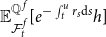 $\mathbb{E}_{\mathcal{F}^{f}_t}^{\mathbb{Q}^{\,f}}[e^{-\int _{t}^u r_s \mathrm{d}s}h]$
, one might naturally consider applying this same methodology to the broader class of hybrid life payoffs
$\mathbb{E}_{\mathcal{F}^{f}_t}^{\mathbb{Q}^{\,f}}[e^{-\int _{t}^u r_s \mathrm{d}s}h]$
, one might naturally consider applying this same methodology to the broader class of hybrid life payoffs $H \in \mathcal{H}_u$
by defining the following
$H \in \mathcal{H}_u$
by defining the following $t^u$
-financial valuation operator
$t^u$
-financial valuation operator $\pi _{t}^{u,f}$
 \begin{equation} \pi _t^{u,f}(H|\mathcal{F}_t)\overset {\Delta }{=}\mathbb{E}_{\mathcal{F}_t}^{\mathbb{P}^{a} \times \mathbb{Q}^{\,f}}\big[e^{-\int _{t}^ur_s\textrm {d}s}H\big] , \end{equation}
with $H \in \mathcal{H}_u$
and
$H \in \mathcal{H}_u$
and $0\le t \le u\le T.$
Definition 3 (Market-consistent property). Let $0\le t \le u\le T$
. A
$0\le t \le u\le T$
. A $t^u$
-valuation operator
$t^u$
-valuation operator $\pi _t^{u}$
is market-consistent with respect to the
$\pi _t^{u}$
is market-consistent with respect to the $t^u$
-financial operator
$t^u$
-financial operator $\pi _{t}^{u,f}$
defined in (
6
) if and only if
$\pi _{t}^{u,f}$
defined in (
6
) if and only if
 \begin{align*} \forall h \in \mathcal{H}_u^f,\forall H \in \mathcal{H}_u\;:\; \pi _{t}^{u}(H+h|\mathcal{F}_t)=\pi _{t}^{u}(H|\mathcal{F}_t)+\pi _t^{u,f}(h|\mathcal{F}_t). \end{align*}
On the actuarial front, we assume that establishing actuarial consistency will draw upon two actuarial principles, namely, the standard deviation premium principle and the variance premium principle. Given the stochastic nature of interest rates in our study, we will adopt the framework proposed by Belhouari et al. (Reference Belhouari, Deelstra and Devolder2025), albeit with minor modifications.
The standard deviation premium principle is
 \begin{equation} \pi _{t}^{u,SD}[H|\mathcal{F}_t]=\mathbb{E }_{\mathcal{F}_t}^{\mathbb{P}^a\times \mathbb{Q}^{\,f}}\big[e^{-\int _{t}^ur_s\textrm {d}s} H\big]+ \alpha _t\sqrt {\mathbb{V}_{\mathcal{F}_t}[H]} \times \sqrt {u-t}\times P(t,u), \end{equation}
for $0\le t \le u\le T$
,
$0\le t \le u\le T$
, $ H \in \mathcal{H}_u,$
and
$ H \in \mathcal{H}_u,$
and $\alpha _{t}\gt 0$
is the portion of the load used at time
$\alpha _{t}\gt 0$
is the portion of the load used at time $t$
. The standard deviation term is multiplied by the factor
$t$
. The standard deviation term is multiplied by the factor $\sqrt {u-t}$
; this small change is necessary to solve the dimensionality problem that arises from the different time-scales produced by the expectation and the standard deviation, see Pelsser and Ghalehjooghi (Reference Pelsser and Ghalehjooghi2016). The variance premium principle is
$\sqrt {u-t}$
; this small change is necessary to solve the dimensionality problem that arises from the different time-scales produced by the expectation and the standard deviation, see Pelsser and Ghalehjooghi (Reference Pelsser and Ghalehjooghi2016). The variance premium principle is
 \begin{equation} \pi _{t}^{u,V}[H|\mathcal{F}_t]=\mathbb{E }_{\mathcal{F}_t}^{\mathbb{P}^a\times \mathbb{Q}^{\,f}}\big[e^{-\int _{t}^ur_s\textrm {d}s}H\big]+ \gamma _{t}\times \mathbb{V}_{\mathcal{F}_t}[H]\times P(t,u), \end{equation}
for $0\le t \le u\le T$
,
$0\le t \le u\le T$
, $ H \in \mathcal{H}_u.$
As the expectation is linear in monetary units while the variance is quadratic, a dimensional mismatch arises. To address this, we define
$ H \in \mathcal{H}_u.$
As the expectation is linear in monetary units while the variance is quadratic, a dimensional mismatch arises. To address this, we define $\gamma _t \gt 0$
as a loading parameter expressed in inverse monetary units. In our market-fair valuation context, detached from specific regulatory constraints, the insurer sets the parameters
$\gamma _t \gt 0$
as a loading parameter expressed in inverse monetary units. In our market-fair valuation context, detached from specific regulatory constraints, the insurer sets the parameters $\alpha _t$
and
$\alpha _t$
and $\gamma _t$
based on its own risk appetite.
$\gamma _t$
based on its own risk appetite.
Definition 4 (Actuarial-consistent property). Let $0\le t \le u\le T$
. A
$0\le t \le u\le T$
. A $t^u$
-valuation operator
$t^u$
-valuation operator $\pi _{t}^{u}$
is actuarial-consistent with respect to the
$\pi _{t}^{u}$
is actuarial-consistent with respect to the $t^u$
-actuarial operator
$t^u$
-actuarial operator $\pi _{t}^{u,a}$
if and only if
$\pi _{t}^{u,a}$
if and only if $\forall g\in \mathcal{H}_u^{a}$
,
$\forall g\in \mathcal{H}_u^{a}$
,
 \begin{align*} \pi _{t}^{u}(g|\mathcal{F}_t)=\pi _t^{u,a}(g|\mathcal{F}_t), \end{align*}

Definition 5 ( $t^T$
-Fair valuation). Let
$t^T$
-Fair valuation). Let $0\le t \le u\le T$
. A
$0\le t \le u\le T$
. A $t^u$
-fair valuation is a
$t^u$
-fair valuation is a $t^u$
-valuation operator that is both market-consistent and actuarial-consistent.
$t^u$
-valuation operator that is both market-consistent and actuarial-consistent.
Definition 6 (Market-consistent dynamic valuation). A market-consistent dynamic valuation is a dynamic valuation $(\pi _{t}^{u})_{0\le t \le u\le T}$
, where for each
$(\pi _{t}^{u})_{0\le t \le u\le T}$
, where for each $0\le t \le u\le T$
,
$0\le t \le u\le T$
, $\pi _{t}^{u}$
is a
$\pi _{t}^{u}$
is a $t^u$
-market-consistent valuation operator.
$t^u$
-market-consistent valuation operator.
Definition 7 (Actuarial-consistent dynamic valuation). An actuarial-consistent dynamic valuation is a dynamic valuation $(\pi _{t}^{u})_{0\le t \le u\le T}$
, where for each
$(\pi _{t}^{u})_{0\le t \le u\le T}$
, where for each $0\le t \le u\le T$
,
$0\le t \le u\le T$
, $\pi _{t}^{u}$
is an
$\pi _{t}^{u}$
is an $t^u$
-actuarial-consistent valuation operator.
$t^u$
-actuarial-consistent valuation operator.
Definition 8 (Fair dynamic valuation). A fair dynamic valuation is a dynamic valuation $(\pi _{t}^{u})_{0\le t \le u\le T}$
, where for each
$(\pi _{t}^{u})_{0\le t \le u\le T}$
, where for each $0\le t \le u\le T$
,
$0\le t \le u\le T$
, $\pi _{t}^{u}$
is a
$\pi _{t}^{u}$
is a $t^u$
-fair valuation.
$t^u$
-fair valuation.
Note that the operator $\pi _{t}^{u,f}$
is market-consistent but not actuarial-consistent. In contrast, the standard deviation
$\pi _{t}^{u,f}$
is market-consistent but not actuarial-consistent. In contrast, the standard deviation $\pi _{t}^{u,SD}$
and variance
$\pi _{t}^{u,SD}$
and variance $\pi _{t}^{u,V}$
premium principles are actuarial-consistent but do not satisfy market-consistency. Consequently, the remainder of this paper focuses on the Three-step method, which defines a fair valuation operator for assessing hybrid products.
$\pi _{t}^{u,V}$
premium principles are actuarial-consistent but do not satisfy market-consistency. Consequently, the remainder of this paper focuses on the Three-step method, which defines a fair valuation operator for assessing hybrid products.
2.3 Three-step decomposition in a dynamic setting
Within the scope of our study, we investigate the Three-step method introduced in Deelstra et al. (Reference Deelstra, Devolder, Gnameho and Hieber2020). To this end, we extend the natural dynamic approach of the Three-step decomposition. We consider the aggregate hybrid payoff for the insured entities, outlined as
 \begin{equation} _{t}H_{u}^{c}=h(S_{u})\sum _{j=1}^{N_{t}}g(\tau _{j}), \end{equation}
where $0\le t \le u\le T$
,
$0\le t \le u\le T$
, $g:\;]0,\infty [\rightarrow [0,\infty [$
and
$g:\;]0,\infty [\rightarrow [0,\infty [$
and $h:\;]0,\infty [\rightarrow [0,\infty [$
are two
$h:\;]0,\infty [\rightarrow [0,\infty [$
are two $\mathcal{F}^{a}_u$
-measurable functions and
$\mathcal{F}^{a}_u$
-measurable functions and $\mathcal{F}^{f}_u$
-measurable, respectively.Footnote 5 We decompose
$\mathcal{F}^{f}_u$
-measurable, respectively.Footnote 5 We decompose $\frac {_{t}H_{u}^c}{N_t}\times {\unicode {x1D7D9}_{N_{t}\gt 0}}$
, with respect to the full spectrum of information, as followsFootnote 6
$\frac {_{t}H_{u}^c}{N_t}\times {\unicode {x1D7D9}_{N_{t}\gt 0}}$
, with respect to the full spectrum of information, as followsFootnote 6
 \begin{equation} _{t}H_{u}=\frac {_{t}H_{u}^c}{N_t}\times {\unicode {x1D7D9}_{N_{t}\gt 0}}=\ _tH_u^{1}+\ _tH_u^{2} + \ _tH_u^{3}, \end{equation}
where
 \begin{equation} _tH_u^{1}\overset {\Delta }{=}\mathbb{E}_{\mathcal{F}_{t}\lor \mathcal{F}_{u}^f}[{}_{t}H_{u}]=\frac {\sum _{j=1}^{N_t}\mathbb{E}_{\mathcal{F}_t}[g(\tau _j)]h(S_{u})}{N_t}\times {\unicode {x1D7D9}_{N_{t}\gt 0}} . \end{equation}
 \begin{equation} _tH_u^{2} \overset {\Delta }{=}\ _{t}H_{u}-\mathbb{E}_{\mathcal{F}_{t}\lor \mathfrak{S}_{u} \lor \mathcal{F}_{u}^f}[{}_{t}H_{u}]=\frac {\sum _{j=1}^{N_t}(g(\tau _j)-\mathbb{E}_{\mathcal{F}_t\lor \mathfrak{S}_u}[g(\tau _j)])h(S_{u})}{N_t} \times {\unicode {x1D7D9}_{N_{t}\gt 0}}. \end{equation}
 \begin{align} {}_tH_u^{3} &\overset {\Delta }{=} \mathbb{E}_{\mathcal{F}_{t}\lor \mathfrak{S}_{u} \lor \mathcal{F}_{u}^f}[{}_{t}H_{u}] - \mathbb{E}_{\mathcal{F}_{t}\lor \mathcal{F}_{u}^f}[{}_{t}H_{u}]\nonumber \\ &= \frac {1}{N_t} \sum _{j=1}^{N_t} (\mathbb{E}_{\mathcal{F}_t\lor \mathfrak{S}_u}[g(\tau _j)] - \mathbb{E}_{\mathcal{F}_t}[g(\tau _j)]) h(S_{u}) \, \unicode {x1D7D9}_{N_{t}\gt 0}. \end{align}
The term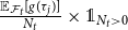 $\frac {\mathbb{E}_{\mathcal{F}_t}[g(\tau _j)]}{N_t}\times {\unicode {x1D7D9}_{N_{t}\gt 0}}$
exhibits
$\frac {\mathbb{E}_{\mathcal{F}_t}[g(\tau _j)]}{N_t}\times {\unicode {x1D7D9}_{N_{t}\gt 0}}$
exhibits $\mathcal{F}_t$
-measurability, then
$\mathcal{F}_t$
-measurability, then $_tH_u^{1}$
is a financial claim; consequently
$_tH_u^{1}$
is a financial claim; consequently $\pi ^{u,f}_{t}$
serves as the suitable operator for its assessment. The component (12) is diversifiable since this assertion holds
$\pi ^{u,f}_{t}$
serves as the suitable operator for its assessment. The component (12) is diversifiable since this assertion holds
 \begin{align*} &_t H_u^2 \Bigl |_{\mathcal{F}_t \lor \mathcal{F}_u^f \lor \mathfrak{S}_u} = \frac {1}{N_t} \sum _{j=1}^{N_t} ( g(\tau _j) - \mathbb{E}_{\mathcal{F}_t \lor \mathfrak{S}_u}[g(\tau _j)]) h(S_u) \Bigl |_{\mathcal{F}_t \lor \mathcal{F}_u^f \lor \mathfrak{S}_u} \\ &\xrightarrow {N_t \to \infty } \mathbb{E} \big[ ( g(\tau _1) - \mathbb{E}_{\mathcal{F}_t \lor \mathfrak{S}_u}[g(\tau _1)] \bigr ) h(S_u) \; |\; \mathcal{F}_t \lor \mathcal{F}_u^f \lor \mathfrak{S}_u \big] = h(S_u)\times 0 =0 \quad \text{a.s.} \end{align*}
Hence, we assess it by applying actuarial premium principles. Furthermore, both the standard deviation premium principle (7) and the variance principle (8) conform to pooling arguments in relation to $_{t}H_{u}^{2}$
. Indeed, they approach a zero value in an asymptotic sense.Footnote 7 Concerning the final part
$_{t}H_{u}^{2}$
. Indeed, they approach a zero value in an asymptotic sense.Footnote 7 Concerning the final part $_tH_u^{3}$
, it represents the systematic risk which is unaffected by both hedging and diversification. To compute its valuation, we propose an Esscher transform following Deelstra et al. (Reference Deelstra, Devolder, Gnameho and Hieber2020), detailed as follows
$_tH_u^{3}$
, it represents the systematic risk which is unaffected by both hedging and diversification. To compute its valuation, we propose an Esscher transform following Deelstra et al. (Reference Deelstra, Devolder, Gnameho and Hieber2020), detailed as follows
 \begin{equation} \pi _{t}^{u,n}( H|\mathcal{F}_t) \overset {\Delta }{=} \mathbb{E}_{\mathcal{F}_t}^{\mathbb{Z}_{\theta }^{a}\times \mathbb{Q}^{\,f}}\big[e^{-\int _{t}^ur_s\textrm {d}s}\times H\big], \end{equation} $H \in \mathcal{H}_u$
,
$H \in \mathcal{H}_u$
, $0\le t \le u\le T$
and
$0\le t \le u\le T$
and
 \begin{equation} \frac {d\mathbb{Z}_{\theta }^a}{d\mathbb{P}^a}\Big |_{\mathcal{F}_t}\overset {\Delta }{=}\frac {e^{\int _{t}^u \theta _{t,u}^{(1)} \lambda _s\textrm {d}s}}{\mathbb{E}_{\mathcal{F}_t}\big[e^{\int _{t}^u \theta _{t,u}^{(1)}\lambda _s\textrm {d}s}\big]}, \end{equation}
The explicit formula for $\theta _{t,u}^{(1)}$
depends on the specified dynamics of stochastic mortality rates and will therefore be provided later; see Subsection 3.2 for further details on this point.
$\theta _{t,u}^{(1)}$
depends on the specified dynamics of stochastic mortality rates and will therefore be provided later; see Subsection 3.2 for further details on this point.
Definition 9 (The dynamic Three-step method). Let $0\le t \le u\le T$
. The dynamic Three-step method is defined by
$0\le t \le u\le T$
. The dynamic Three-step method is defined by
 \begin{align*} \pi _t^{u,3}\big(_{t}H_{u}|\mathcal{F}_t\big)\overset {\Delta }{=}\pi _t^{u,f}\big(_tH_u^{1}|\mathcal{F}_t\big)+\pi _t^{u,a}\big(_tH_u^{2}|\mathcal{F}_t\big)+\pi _t^{u,n}\big(_tH_u^{3}|\mathcal{F}_t\big), \end{align*}
where $\pi _{t}^{u,f}$
is given by (
6
),
$\pi _{t}^{u,f}$
is given by (
6
), $\pi _{t}^{u,a}$
is given by (
7
) or (
8
) and
$\pi _{t}^{u,a}$
is given by (
7
) or (
8
) and $\pi _{t}^{u,n}$
is given by (
14
).
$\pi _{t}^{u,n}$
is given by (
14
).
It is easy to check that the dynamic Three-step method is fair according to our axiomatization.
3. Time-consistent dynamic valuations
3.1 Time consistency properties for financial products
Once a dynamic valuation is defined, the inquiry naturally extends to the temporal behavior of valuations across distinct time instances. The challenge lies in maintaining the hierarchical sequence of position preferences for products evaluated through dynamic valuation to safeguard rational behavior and thereby mitigate the emergence of financial arbitrage opportunities. We will first establish a mathematical formulation of this fundamental property for purely financial products, then broaden the scope to encompass hybrid life Pure Endowment products, with a particular focus on the dynamic Three-step method. Based on Acciaio and Penner (Reference Acciaio and Penner2011), we state the following definition of time-consistency.
Definition 10 (Time-consistent property for financial products). A dynamic valuation $(\pi _{t}^{u})_{0\le t \le u\le T}$
is time-consistent if and only if,
$(\pi _{t}^{u})_{0\le t \le u\le T}$
is time-consistent if and only if, $ \forall 0\le t \le u,v\le T$
,
$ \forall 0\le t \le u,v\le T$
, $\forall \ 0\lt s \le u-t$
,
$\forall \ 0\lt s \le u-t$
, $0\lt s\le v-t$
Footnote
8
,
$0\lt s\le v-t$
Footnote
8
, $\forall$ $h \in \mathcal{H}_u^f$
,
$h \in \mathcal{H}_u^f$
, $g \in \mathcal{H}_v^f$
,
$g \in \mathcal{H}_v^f$
,
 \begin{equation} \pi _{t+s}^{u}[h]\le \pi _{t+s}^{v}[g]\ \Rightarrow \pi _{t}^{u}[h]\le \pi _{t}^{v}[g]. \end{equation}
For instance, the mathematical expectation is a time-consistent dynamic because of the tower rule property. Notably, $(\pi _{t}^{u,f})_{0 \le t \le u \le T}$
is time-consistent. Alternatively, an iteratively backward scheme, closely associated to time-consistency, is frequently used in the literature.
$(\pi _{t}^{u,f})_{0 \le t \le u \le T}$
is time-consistent. Alternatively, an iteratively backward scheme, closely associated to time-consistency, is frequently used in the literature.
Definition 11 (Iterated property for financial products). A dynamic valuation $(\pi _{t}^{u})_{0\le t \le u\le T}$
is iterated if and only if,
$(\pi _{t}^{u})_{0\le t \le u\le T}$
is iterated if and only if, $ \forall 0\le t \le u\le T$
,
$ \forall 0\le t \le u\le T$
, $\forall 0\lt s\le u-t$
,
$\forall 0\lt s\le u-t$
, $\forall h \in \mathcal{H}_u^f$
,
$\forall h \in \mathcal{H}_u^f$
,
 \begin{equation} \pi _{t}^{t+s} \big[\pi _{t+s}^{u} [h ] \big]=\pi _{t}^{u}[h]. \end{equation}
Remark 1. Each time-consistent dynamic valuation satisfies the equation (17). Moreover, under the monotonicityFootnote 9 hypothesis, Definitions 10 and 11 are equivalent, see details in the Appendix.
Through Definition 11, we can progressively devise a backward-looking procedure in a discrete configuration, enabling, when it is not the case initially, the establishment of time-consistency for dynamic valuations that exhibit monotonicity.
Corollary 1.
Let $\Delta t \in \ ]0,T[$
. Let
$\Delta t \in \ ]0,T[$
. Let $(\pi _{t}^{u})_{0\le t \le u\le T}$
be a dynamic valuation that adheres to monotonicity but not necessarily time-consistency, then the resulting sequence
$(\pi _{t}^{u})_{0\le t \le u\le T}$
be a dynamic valuation that adheres to monotonicity but not necessarily time-consistency, then the resulting sequence $(\tilde {\pi _{t}})_{t}$
Footnote
10
constructed according to the outlined procedure satisfies time-consistency.
$(\tilde {\pi _{t}})_{t}$
Footnote
10
constructed according to the outlined procedure satisfies time-consistency.
-
1. First step.
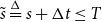
\begin{align*} \tilde {\pi }_{T-\Delta t}[h]=\pi _{T-\Delta t}[h]. \end{align*}
-
2. Second step. For
$s=\Delta t,\ 2\Delta t,\ 3\Delta t,\ \ldots$
and while
$\tilde {s}\overset {\Delta }{=}s+\Delta t \le T$
where
\begin{align*} \tilde {\pi }_{T-\tilde {s}}[h]=\pi _{T-\tilde {s}}^{T-s} [\tilde {\pi }_{T-s} [h ] ], \end{align*}
$h \in \mathcal{H}_T^f.$




The following subsection will examine time-consistency for hybrid-life Pure Endowment products. Fair – i.e., market-actuarial consistent – valuation operators for these products are frequently neither monotone nor time-consistent; see, for example, the operator of Møller (Reference Møller2002), the Two-step operator of Pelsser and Stadje (Reference Pelsser and Stadje2014), the Two-step operator of Barigou et al. (Reference Barigou, Chen and Dhaene2019), and the Three-step operator considered in our work. Consequently, the usual equivalence between the two versions of time-consistency (the two formulations in Definitions 10 and 11) no longer holds. Nonetheless, such counterexamples typically arise only in extreme contexts and thus have limited practical relevance. For the remainder of the paper, we will therefore adopt the iterative version of time-consistency as the reference definition. Moreover, some contributions in the financial literature consider the formulation presented in Definition 11 as the primary definition of time-consistency; see, for instance, Bion-Nadal (Reference Bion-Nadal2009).
3.2 Time-consistency in hybrid life Pure Endowment products
We investigate a hybrid life insurance product, where the longevity risk corresponds to what is commonly referred to in the literature as a Pure Endowment product. The benefit consists of generating a payment only in case of survival of the insured at a fixed maturity. No payout is made in the event of premature death. For the financial payoff, we consider a broad framework involving any measurable function $h$
of the financial investment fund. Formally, the collective payoff for a maturity
$h$
of the financial investment fund. Formally, the collective payoff for a maturity $u\le T$
is
$u\le T$
is
 \begin{equation} _{t}H_u^{c}=\left(\sum _{j=1}^{N_t}{\unicode {x1D7D9}_{\tau _{j}\gt u}}\right)\times h(S_u). \end{equation}
Under mortality risk, the number of survivors decreases over time from the initial instant to maturity. This necessitates ensuring price equilibrium across different time points, taking into account the number of survivors at each point in time. When dealing with such hybrid life Pure Endowment products, this adjustment should be integrated into the iterative time consistency property specified in Definition 11. Hence, Definition 11 extends to hybrid life Pure Endowment products as follows.
Definition 12 (Time-consistency for hybrid life Pure Endowment products). Consider the collective payoff given by (
18
), and let $_{t}H_{u}$
be its individual payoff. A dynamic valuation
$_{t}H_{u}$
be its individual payoff. A dynamic valuation $(\pi _{t}^{u})_{0\le t \le u\le T}$
is time-consistent if and only if,
$(\pi _{t}^{u})_{0\le t \le u\le T}$
is time-consistent if and only if,
 \begin{equation} \pi _{t}^{t+s}\left[\frac {N_{t+s}}{N_t}\pi _{t+s}^{u} [{}_{t+s}H_{u} ]\right]=\pi _{t}^{u}[{}_{t}H_{u}]. \end{equation}
In the context of hybrid products embedding non-tradable longevity risk, time-inconsistent valuation does not give rise to exploitable arbitrage opportunities, as the difficulty of trading such risk prevents their effective implementation. Nevertheless, time consistency remains essential for insurers’ rational decision-making about the products they offer, as it ensures that choices made today remain viable over time.
3.3 The Three-step method time-consistent dynamic for hybrid life Pure Endowment products
Definition 13 (Time-consistency of the Three-step method). Consider the collective payoff given by (
18
). Let $_{t}H_u^{1}$
,
$_{t}H_u^{1}$
, $_{t}H_u^{2}$
, and
$_{t}H_u^{2}$
, and $_{t}H_u^{3}$
be its Three-step decomposition, as defined respectively in (
10
), (
11
), and (
12
). Then, the dynamic Three-step method is time-consistent if and only if the equation below holds
$_{t}H_u^{3}$
be its Three-step decomposition, as defined respectively in (
10
), (
11
), and (
12
). Then, the dynamic Three-step method is time-consistent if and only if the equation below holds
 \begin{align} &\pi _{t}^{t+s,3}\left[\frac {N_{t+s}}{N_{t}}\times \left(\pi _{t+s}^{u,f}\big[{}_{t+s}H_{u}^1\big]+\pi _{t+s}^{u,a}\big[{}_{t+s}H_{u}^{2}\big]+\pi _{t+s}^{u,n}\big[{}_{t+s}H_{u}^{3}\big] \right) \right]\nonumber\\[3pt] &\quad =\pi _{t}^{u,f}\big[{}_{t}H_u^{1}\big]+\pi _{t}^{u,a}\big[{}_{t}H_u^{2}\big]+\pi _{t}^{u,n}\big[{}_{t}H_u^{3}\big],\end{align}
for all $ 0\le t \le u\le T, 0\lt s\le u-t$
.
$ 0\le t \le u\le T, 0\lt s\le u-t$
.
We cannot proceed by applying the iterative time-consistency formula to each Three-step component in isolation. This comes from the fact that a unique initial decomposition at maturity $u$
cannot be preserved as time progresses. For instance, while the risk
$u$
cannot be preserved as time progresses. For instance, while the risk $_{t+s}H_{u}^1$
is hedgeable at time
$_{t+s}H_{u}^1$
is hedgeable at time $t+s$
, the risk
$t+s$
, the risk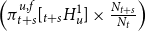 $\Big (\pi _{t+s}^{u,f}[{}_{t+s}H_{u}^{1}]\times \frac {N_{t+s}}{N_{t}}\Big )$
ceases to be hedgeable at time
$\Big (\pi _{t+s}^{u,f}[{}_{t+s}H_{u}^{1}]\times \frac {N_{t+s}}{N_{t}}\Big )$
ceases to be hedgeable at time $t$
. Consequently, applying the financial operator
$t$
. Consequently, applying the financial operator $\pi _{t}^{t+s,f}$
to
$\pi _{t}^{t+s,f}$
to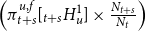 $\Big (\pi _{t+s}^{u,f}[{}_{t+s}H_{u}^{1}]\times \frac {N_{t+s}}{N_{t}}\Big )$
would be inappropriate. Likewise, there is no assurance that the risk
$\Big (\pi _{t+s}^{u,f}[{}_{t+s}H_{u}^{1}]\times \frac {N_{t+s}}{N_{t}}\Big )$
would be inappropriate. Likewise, there is no assurance that the risk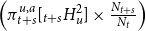 $\Big (\pi _{t+s}^{u,a}[{}_{t+s}H_{u}^{2}]\times \frac {N_{t+s}}{N_{t}}\Big )$
will remain diversifiable at time
$\Big (\pi _{t+s}^{u,a}[{}_{t+s}H_{u}^{2}]\times \frac {N_{t+s}}{N_{t}}\Big )$
will remain diversifiable at time $t$
, excluding its revaluation through a
$t$
, excluding its revaluation through a $t^{t+s}$
-actuarial operator. Viewed from time
$t^{t+s}$
-actuarial operator. Viewed from time $t$
,
$t$
,
 \begin{equation} _{t}LY_{t+s}\overset {\Delta }{=}\frac {N_{t+s}}{N_{t}}\times \big(\pi _{t+s}^{u,f}\big[{}_{t+s}H_{u}^1\big]+\pi _{t+s}^{u,a}\big[{}_{t+s}H_{u}^{2}\big]+\pi _{t+s}^{u,n}\big[{}_{t+s}H_{u}^{3}\big] \big) \end{equation}
is a payoff that matures at $t+s$
. Hence, once again, it must be decomposed into a hedgeable component, a diversifiable component, and a systematic component to apply the Three-step method and determine the valuation at time
$t+s$
. Hence, once again, it must be decomposed into a hedgeable component, a diversifiable component, and a systematic component to apply the Three-step method and determine the valuation at time $t.$
$t.$
As an introductory step, we aim to assess the time-consistency of the Three-step approach, disregarding the diversifiable risk. This results in the Three-step decomposition being simplified to a ’Two-step’ model, comprising a hedgeable part and a systematic part, as detailed below
 \begin{align*} \left \{ \begin{array}{ll} _{t}H_u^{h}\overset {\Delta }{=}\mathbb{E}_{\mathcal{F}_{t}\lor \mathcal{F}_{u}^f}[{}_{t}H_u]=\mathbb{E}_{\mathcal{F}_{t}}\big[e^{-\int _{t}^u \lambda _s\textrm {d}s}\big]\times h(S_u)\times {\unicode {x1D7D9}_{N_{t}\gt 0}},\\[3pt] _{t}H_u^{sy}\overset {\Delta }{=}\ _{t}H_u-\mathbb{E}_{\mathcal{F}_{t}\lor \mathcal{F}_{u}^f}[{}_{t}H_u]=\left (\dfrac {N_u}{N_{t}}-\mathbb{E}_{\mathcal{F}_{t}}\big[e^{-\int _{t}^u \lambda _s\textrm { d}s}\big]\right )\times h(S_u)\times {\unicode {x1D7D9}_{N_{t}\gt 0}}. \end{array} \right \} \end{align*}
Therefore, $\pi _{t}^{u,3}[{}_{t}H_{u}]$
introduced in Definition 9, is reduced to
$\pi _{t}^{u,3}[{}_{t}H_{u}]$
introduced in Definition 9, is reduced to
 \begin{equation} \pi _{t}^{u,2}[{}_{t}H_{u}]\overset {\Delta }{=}\pi _{t}^{u,f}\big[{}_{t}H_{u}^h\big]+\pi _{t}^{u,n}\big[{}_{t}H_{u}^{sy}\big]. \end{equation}
Lemma 1.
The dynamic $(\pi _{t}^{u,2})_{0\le t \le u\le T}$
is time-consistent; consequently, its time-consistent valuation is given, by the one-period valuation, as follows
$(\pi _{t}^{u,2})_{0\le t \le u\le T}$
is time-consistent; consequently, its time-consistent valuation is given, by the one-period valuation, as follows
 \begin{align*} \tilde {\pi }_{t}^{2}[{}_{t}H_T|\mathcal{F}_{t}]=\pi _{t}^{2}[{}_{t}H_T|\mathcal{F}_{t}]=\mathbb{E}_{\mathcal{F}_{t}}^{\mathbb{Q}^{\,f}}\big[e^{-\int _{t}^T r_v\textrm {d}v}h(S_T)\big]\times \mathbb{E}_{\mathcal{F}_{t}}^{\mathbb{Z}_{\theta }^{a}}\big[e^{-\int _{t}^T \lambda _v\textrm {d}v}\big], \end{align*}
with $t \in [0,T].$
Proof. See the Appendix.
Next, we include the diversifiable risk into the previous decomposition, finding the full Three-step decomposition as provided below
 \begin{align*} \left \{ \begin{array}{ll} _{t}H_u^{1}=\mathbb{E}_{\mathcal{F}_{t}}\big[e^{-\int _{t}^u \lambda _s\textrm {d}s}\big]\times h(S_u)\times {\unicode {x1D7D9}_{N_{t}\gt 0}},\\[5pt] _{t}H_u^{2}=\left (\dfrac {N_u}{N_{t}}-e^{-\int _{t}^u \lambda _s\textrm {d}s}\right )\times h(S_u)\times {\unicode {x1D7D9}_{N_{t}\gt 0}},\\[5pt] _{t}H_u^{3}=\big(e^{-\int _{t}^u \lambda _s\textrm {d}s}-\mathbb{E}_{\mathcal{F}_{t}}\big[e^{-\int _{t}^u \lambda _s\textrm {d}s}\big]\big)\times h(S_u)\times {\unicode {x1D7D9}_{N_{t}\gt 0}}. \end{array} \right \} \end{align*}
Lemma 2.
The dynamic Three-step method $(\pi _{t}^{u,3})_{0\le t \le u\le T}$
introduced in Definition
9
, is not time-consistent.
$(\pi _{t}^{u,3})_{0\le t \le u\le T}$
introduced in Definition
9
, is not time-consistent.
Proof. See the Appendix.
Since the dynamic Three-step method is not time-consistent, we strive to iteratively construct a sequence of time-consistent valuations by applying Corollary1 in line with Definition 13.
Corollary 2.
Let $\Delta t \in ]0,T[$
. Let
$\Delta t \in ]0,T[$
. Let $(\pi _{t}^{u,3})_{0\le t \le u\le T}$
be the dynamic Three-step method defined in Definition
9
, then the resulting sequence
$(\pi _{t}^{u,3})_{0\le t \le u\le T}$
be the dynamic Three-step method defined in Definition
9
, then the resulting sequence $(\tilde {\pi }_{t}^{3})_{t}$
constructed according to the outlined procedure is time-consistent
$(\tilde {\pi }_{t}^{3})_{t}$
constructed according to the outlined procedure is time-consistent
-
1. First step.
\begin{align*} \tilde {\pi }^{3}_{T-\Delta t}[{}_{T-\Delta t}H_T]=\pi ^{3}_{T-\Delta t}[{}_{T-\Delta t}H_T]. \end{align*}
-
2. Second step. For
$s=\Delta t,\ 2\Delta t,\ 3\Delta t,\ \ldots$
and while
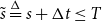
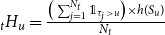
$\tilde {s}\overset {\Delta }{=}s+\Delta t \le T$
(23)for
\begin{equation} \tilde {\pi }^{3}_{T-\tilde {s}}[{}_{T-\tilde {s}}H_T]=\pi _{T-\tilde {s}}^{T-s,3}\left [\frac {N_{T-s}}{N_{T-\tilde {s}}}\times \tilde {\pi }^{3}_{T-s} [{}_{T-s}H_T ]\right ], \end{equation}
$_{t}H_{u}=\frac {\big (\sum _{j=1}^{N_t}{\unicode {x1D7D9}_{\tau _{j}\gt u}}\big )\times h(S_u)}{N_t}$
and where
$0\le t \le u\le T.$




To derive explicit time-consistent valuations based on Corollary2, it is essential to specify the dynamics of $(\lambda _{t})_{0\leq t \leq T}$
,
$(\lambda _{t})_{0\leq t \leq T}$
, $(S_{t})_{0\leq t \leq T}$
and
$(S_{t})_{0\leq t \leq T}$
and $(r_{t})_{0 \leq t \leq T}.$
Under
$(r_{t})_{0 \leq t \leq T}.$
Under $\mathbb{P}^a$
, the stochastic mortality rate
$\mathbb{P}^a$
, the stochastic mortality rate $\lambda _{t}$
follows a stochastic solution of the following equation commonly recognized as the Ornstein–Uhlenbeck intensity process (see Luciano & Vigna, Reference Luciano and Vigna2008)
$\lambda _{t}$
follows a stochastic solution of the following equation commonly recognized as the Ornstein–Uhlenbeck intensity process (see Luciano & Vigna, Reference Luciano and Vigna2008)
 \begin{align*} d\lambda _t=\mu _m\lambda _t dt+\sigma _m dW_m(t), \end{align*}
where $(W_{m}(t))_{t\ge 0}$
is a Brownian motion and
$(W_{m}(t))_{t\ge 0}$
is a Brownian motion and $\mu _m\gt 0$
,
$\mu _m\gt 0$
, $\sigma _m\gt 0.$
Thus, for
$\sigma _m\gt 0.$
Thus, for $0\le t \le u\le T$
,
$0\le t \le u\le T$
, $\ _{u-t}p_{x+t}=e^{-\lambda _{t}l_{t,u}+\frac {1}{2}s_{t,u}^2},$
where
$\ _{u-t}p_{x+t}=e^{-\lambda _{t}l_{t,u}+\frac {1}{2}s_{t,u}^2},$
where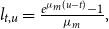 $l_{t,u}=\frac {e^{\mu _{m}(u-t)}-1}{\mu _{m}},$
and
$l_{t,u}=\frac {e^{\mu _{m}(u-t)}-1}{\mu _{m}},$
and $s_{t,u}^2=\frac {\sigma _m^2}{2\mu _m^3}(1-e^{\mu _m(u-t)})^2+\frac {\sigma _m^2}{\mu _m^2}((u-t)-\frac {e^{\mu _m(u-t)}-1}{\mu _m}).$
The parameter
$s_{t,u}^2=\frac {\sigma _m^2}{2\mu _m^3}(1-e^{\mu _m(u-t)})^2+\frac {\sigma _m^2}{\mu _m^2}((u-t)-\frac {e^{\mu _m(u-t)}-1}{\mu _m}).$
The parameter $\theta _{t,u}^{(1)}$
present in (15) is adjusted in accordance with the Cost of Capital approach detailed in Belhouari et al. (Reference Belhouari, Deelstra and Devolder2025), producing
$\theta _{t,u}^{(1)}$
present in (15) is adjusted in accordance with the Cost of Capital approach detailed in Belhouari et al. (Reference Belhouari, Deelstra and Devolder2025), producing $\theta _{t,u}^{(1)}=\frac {-0.16}{s_{t,u}}.$
The dynamics of the couple stochastic investment fund and stochastic interest rates will be characterized using the following Black-Scholes-Vasicek model, described under $\mathbb{P}^f$
by
$\mathbb{P}^f$
by
 \begin{align*} \left \{ \begin{array}{ll} dr_t=(b-ar_t)dt+\sigma _r\overset {\sim }{dW}_r(t),\\ dS_t=\mu _S S_tdt+S_t\sigma _S(\rho \overset {\sim }{dW}_r(t)+\sqrt {1-\rho ^2}\overset {\sim }{dW}_S(t)). \end{array} \right \}\!. \end{align*}
where $(\tilde {W}_{S}(t))_{t\ge 0}$
is a Brownian motion independent from
$(\tilde {W}_{S}(t))_{t\ge 0}$
is a Brownian motion independent from $(\tilde {W}_{r}(t))_{t\ge 0}$
,
$(\tilde {W}_{r}(t))_{t\ge 0}$
, $a$
is the constant speed of mean reversion,
$a$
is the constant speed of mean reversion, $b$
represents a strictly positive scalar such that the ratio
$b$
represents a strictly positive scalar such that the ratio $\frac {b}{a}$
is the long-term mean value and
$\frac {b}{a}$
is the long-term mean value and $\sigma _r$
is the constant volatility of interest rates.
$\sigma _r$
is the constant volatility of interest rates. $\mu _S$
is the instantaneous return of
$\mu _S$
is the instantaneous return of $(S_t)_{t\ge 0}$
,
$(S_t)_{t\ge 0}$
, $\sigma _S$
is the volatility of the financial investment fund, and
$\sigma _S$
is the volatility of the financial investment fund, and $\rho$
defines the correlation between the financial investment fund and interest rates. Switching to the risk-neutral probability involves the application of Girsanov’s theorem, which defines the Brownian motions
$\rho$
defines the correlation between the financial investment fund and interest rates. Switching to the risk-neutral probability involves the application of Girsanov’s theorem, which defines the Brownian motions $(W_r(t))_{t}$
and
$(W_r(t))_{t}$
and $(W_S(t))_{t}$
in the following manner
$(W_S(t))_{t}$
in the following manner $\mathbb{P}^f$
 \begin{align*} \left \{ \begin{array}{ll} W_r(t)\overset {\Delta }{=}\overset {\sim }{W}_r(t)-\nu t,\\ W_S(t)\overset {\Delta }{=}\overset {\sim }{W}_S(t)+\int _{0}^t \left(\dfrac {\mu _S-r_u}{\sqrt {1-\rho ^2}\sigma _S}+\dfrac {\nu \rho }{\sqrt {1-\rho ^2}}\right)\,du. \end{array} \right \}\!. \end{align*}
Drawing upon this, the Radon-Nikodym derivative of $\mathbb{Q}^{\,f}$
with respect to
$\mathbb{Q}^{\,f}$
with respect to $\mathbb{P}^f$
is
$\mathbb{P}^f$
is
 \begin{align*} \frac {d\mathbb{Q}^{\,f}}{d\mathbb{P}^f}\Big |_{\mathcal{F}_t}=e^{\nu \overset {\sim }{W}_r(T)-\int _{t}^T \Big(\frac {\mu _S-r_u}{\sqrt {1-\rho ^2}\sigma _S}+\frac {\nu \rho }{\sqrt {1-\rho ^2}}\Big)\,d\overset {\sim }{W}_S(u)-\frac {1}{2}\int _{t}^T \Big(\nu ^2+\Big(\frac {\mu _S-r_u}{\sqrt {1-\rho ^2}\sigma _S}+\frac {\nu \rho }{\sqrt {1-\rho ^2}}\Big)^2\Big)\,du}. \end{align*}
Hence, the following dynamics are obtained under $\mathbb{Q}^{\,f}$
 \begin{align*} \left \{ \begin{array}{ll} dr_t=(\theta -ar_t)dt+\sigma _r dW_r(t),\\ dS_t=r_tS_tdt+S_t\sigma _S(\rho dW_r(t)+\sqrt {1-\rho ^2}dW_S(t)), \end{array} \right . \end{align*}
with $\theta =b+\sigma _{r}\nu .$
3.4 The backward scheme in a dual-iteration approach
The achievement of closed forms through the recursive equation (23) with a substantial number of iterations, given the stochastic risks on both the financial and mortality fronts, as assumed in our study, poses a formidable challenge, if not an unattainable one. To simplify the problem, we consider two periods $[0,b]$
and
$[0,b]$
and $[b,T]$
in a constant interest rate framework,Footnote 11 and where we set
$[b,T]$
in a constant interest rate framework,Footnote 11 and where we set $h(S_u)=1$
. In this case, we are delving into the purely actuarial, Pure Endowment product. Owing to the requirements of derivation and computation, we will use the variance premium principle, defined in (8), as the operator for evaluating the diversifiable risk component of the Three-step method. This choice enables the derivation of a closed-form solution, unlike the standard deviation premium principle. In light of the newly introduced denotations
$h(S_u)=1$
. In this case, we are delving into the purely actuarial, Pure Endowment product. Owing to the requirements of derivation and computation, we will use the variance premium principle, defined in (8), as the operator for evaluating the diversifiable risk component of the Three-step method. This choice enables the derivation of a closed-form solution, unlike the standard deviation premium principle. In light of the newly introduced denotations
 \begin{align*} &\tilde {_{i}f_j}=e^{-i\lambda _{0}l_{b,T}e^{\mu _m b}+j\frac {(e^{\mu _{m}b}+1)}{2}\frac {l_{b,T}^{2}l_{0,b}\sigma _{m}^{2}}{2}+j\frac {\theta _{0,b}^{(1)}l_{0,b}^2l_{b,T}\sigma _{m}^2}{2}},&\\ &_{i}f^{j}_{k}=e^{-i\lambda _{0}l_{0,b}+j\frac {l_{b,T}l_{0,b}^{2}\sigma _{m}^{2}}{2}+k\frac {1}{2}s_{0,b}^{2}},& \end{align*}
we hereby present the following lemma.
Lemma 3.
The Three-step valuation of the Pure Endowment product at the instant $b$
is
$b$
is $\tilde {\pi }_{b}^{3}[{}_{b}H_{T}|\mathcal{F}_{b}]=P(b,T)\Big (e^{-\lambda _{b}l_{b,T}+\frac {1}{2}s_{b,T}^2} e^{-\theta _{b,T}^{(1)} s_{b,T}^2}+\gamma _{b}\times \frac {e^{-\lambda _{b}l_{b,T}+\frac {1}{2}s_{b,T}^2}-e^{-2\lambda _{b}l_{b,T}+2s_{b,T}^2}}{N_b}\Big ).$
While the time-consistent valuation at the instant
$\tilde {\pi }_{b}^{3}[{}_{b}H_{T}|\mathcal{F}_{b}]=P(b,T)\Big (e^{-\lambda _{b}l_{b,T}+\frac {1}{2}s_{b,T}^2} e^{-\theta _{b,T}^{(1)} s_{b,T}^2}+\gamma _{b}\times \frac {e^{-\lambda _{b}l_{b,T}+\frac {1}{2}s_{b,T}^2}-e^{-2\lambda _{b}l_{b,T}+2s_{b,T}^2}}{N_b}\Big ).$
While the time-consistent valuation at the instant $0$
is
$0$
is
 \begin{align*} \tilde {\pi }_{0}^{3}[{}_{0}H_{T}|\mathcal{F}_{0}]=\Gamma ^{(h,sy)}_{0}+\Gamma ^{(div)}_{0}, \end{align*}
where
 \begin{align*} & \Gamma ^{(h,sy)}_{0}=P(0,T)\left(e^{-\lambda _{0}l_{0,T}-s_{0,T}^2(\theta _{0,T}^{(1)}-\frac {1}{2})}+\gamma _{b}\frac {e^{\frac {1}{2}s_{b,T}^2}\tilde {_{1}f_1}-e^{2s_{b,T}^2}\tilde {_{2}f_4}}{n}\right),&\\ & \Gamma ^{(div)}_{0}=\frac {1}{n}\times \gamma _{0}\times P(0,b)P(b,T)^{2} \times e^{-2s_{b,T}^{2}\big(\theta _{b,T}^{(1)}-\frac {1}{2}\big)}\big({}_{1}f^{2}_{1}- \ _{2}f^{8}_{4}\big),&\\ &\theta _{b,T}^{(1)}=\frac {-0.16}{s_{b,T}},&\\ &\theta _{0,b}^{(1)}=\frac {-0.16}{s_{0,b}}.& \end{align*}
Proof. See the Appendix.
A notable aspect is that the aggregated non-diversifiable risks, including systematic and hedgeable components of the time-consistent formula at time $0$
, incorporate loading terms arising from the valuation of the diversifiable component at time
$0$
, incorporate loading terms arising from the valuation of the diversifiable component at time $b$
; as shown in
$b$
; as shown in $\Gamma ^{(h,sy)}_{0}.$
This implies that, during the backward scheme, the valuation of the diversifiable component from the prior iteration impacts the valuation of the subsequent non-diversifiable components. Moreover, observe that, under perfect diversification of the portfolio, the diversifiable risk disappears. Correspondingly, the closed-form Three-step time-consistent price
$\Gamma ^{(h,sy)}_{0}.$
This implies that, during the backward scheme, the valuation of the diversifiable component from the prior iteration impacts the valuation of the subsequent non-diversifiable components. Moreover, observe that, under perfect diversification of the portfolio, the diversifiable risk disappears. Correspondingly, the closed-form Three-step time-consistent price $\tilde {\pi }_{0}^{3}[{}_{0}H_{T}|\mathcal{F}_{0}]$
in Lemma3 converges to the Two-step static price, where it reduces to the best estimate, i.e.,
$\tilde {\pi }_{0}^{3}[{}_{0}H_{T}|\mathcal{F}_{0}]$
in Lemma3 converges to the Two-step static price, where it reduces to the best estimate, i.e., $ (P(0,T)\times e^{-\lambda _{0}l_{0,T}-s_{0,T}^2(\theta _{0,T}^{(1)}-\frac {1}{2})})$
; thereby explicitly confirming that the diversifiable risk component operates to undermine time-consistency.
$ (P(0,T)\times e^{-\lambda _{0}l_{0,T}-s_{0,T}^2(\theta _{0,T}^{(1)}-\frac {1}{2})})$
; thereby explicitly confirming that the diversifiable risk component operates to undermine time-consistency.
4. Partial differential equation for the Three-step method time-consistent dynamic
4.1 Derivation
In the preceding section, several simplistic measures were used to derive the time-consistent valuation across two periods. To comprehensively unveil the repercussions of time consistency on pricing, a more sophisticated numerical approach surpassing two iterations is imperative. This section focuses on studying the continuous-time limit of the Three-step method when integrated into the backward scheme. In order to accomplish this, and following Pelsser and Ghalehjooghi (Reference Pelsser and Ghalehjooghi2016), we will derive PDEFootnote 12 of the Three-step method time-consistent dynamic, incorporating all the stochastic processes of mortality and finance considered in our study. Considering an infinitesimally small time increment $dt$
that tends towards
$dt$
that tends towards $0$
, we position ourselves within the
$0$
, we position ourselves within the $(t, t+dt)$
interval and employ
$(t, t+dt)$
interval and employ
 \begin{equation} \tilde {\pi }_{t}^3=\pi _{t}^{t+dt,3}\left[\frac {N_{t+dt}}{N_t}\times \tilde {\pi }_{t+ dt}^3\right] \end{equation}
This time, we purposefully adopt the standard deviation premium principle to assess the actuarial component of the Three-step method. Interestingly, the variance principle enables the generation of a similar PDE, reflecting also a time-consistent price.
Theorem 1.
Let $t^{(1)}$
be a strictly positive real scalar. The Three-step method time-consistent dynamic
$t^{(1)}$
be a strictly positive real scalar. The Three-step method time-consistent dynamic $(\tilde {\pi }_t^{3})_{t \in [0,T-t^{(1)}]}$
is a solution of the following PDE
$(\tilde {\pi }_t^{3})_{t \in [0,T-t^{(1)}]}$
is a solution of the following PDE
 \begin{equation} r_{t} \tilde {\pi }_{t}^{3} =\Lambda ^{(1)}_{t}+\alpha _{t}\times \sqrt {\Lambda ^{(2)}_{t}}, \end{equation}
with
 \begin{align*} \Lambda ^{(1)}_{t}&=\partial _{t} \tilde {\pi }^{3}_{t}+r_{t}S_{t}\partial _{S} \tilde {\pi }^{3}_{t}+(\theta -ar_{t})\partial _{r} \tilde {\pi }^{3}_{t}+ \left(\overline {\theta _{t,T}^{(1)}}+\mu _m \lambda _t\right)\partial _{\lambda } \tilde {\pi }^{3}_{t}+\frac {1}{2}\sigma _{S}^{2}S_{t}^{2}\partial _{S}^{2}\tilde {\pi }^{3}_{t}+\frac {1}{2} \sigma _{m}^{2}\partial _{\lambda }^{2}\tilde {\pi }^{3}_{t} \\&\quad +\frac {1}{2}\sigma _{r}^{2}\partial _{r}^{2}\tilde {\pi }^{3}_{t} + \rho \sigma _{r}\sigma _{S}S_{t}\partial _{rS}^{2}\tilde {\pi }^{3}_{t}+\big(\tilde {\pi }^{3*}_{t}-\tilde {\pi }_{t}^{3}\big)\lambda _{t},&\\\Lambda ^{(2)}_{t}&=\sigma _{S}^{2}S_{t}^{2}\big(\partial _{S}\tilde {\pi }^{3}_{t}\big)^2+ \sigma_{m}^{2}\big(\partial_{\lambda}\tilde{\pi}^{3}_{t}\big)^2+\sigma _{r}^{2}\big(\partial _{r}\tilde {\pi }^{3}_{t}\big)^2+2\rho \sigma _{S}\sigma _{r}S_{t}\partial _{S}\tilde {\pi }^{3}_{t}\partial _{r}\tilde {\pi }^{3}_{t}+\big(\tilde {\pi }_{t}^{3}-\tilde {\pi }_{t}^{3*}\big)^{2}\lambda _{t},&\\\overline {\theta _{t,T}^{(1)}}&=\theta _{0,T}^{(1)}\sigma _{m}^{2}\times \frac {e^{\mu _{m}(T-t)}-1}{\mu _m},&\\ \tilde {\pi }_{t}^{3*}[.]&=\tilde {\pi }_{t}^{3}[.|N_{t}-1].& \end{align*}
Proof. See the Appendix.
Represented by $\Lambda ^{(1)}_{t}$
, the first component of the PDE captures the time-consistent price of the aggregate replicable and systematic risks. The subsequent part
$\Lambda ^{(1)}_{t}$
, the first component of the PDE captures the time-consistent price of the aggregate replicable and systematic risks. The subsequent part $\Big (\alpha _{t}\times \sqrt {\Lambda ^{(2)}_{t}}\Big )$
, relates to the time-consistent value of the diversifiable risk.
$\Big (\alpha _{t}\times \sqrt {\Lambda ^{(2)}_{t}}\Big )$
, relates to the time-consistent value of the diversifiable risk.
Contrary to the time-consistent case, the static continuous-time valuation framework circumvents the requirement for a PDE. Indeed, a closed-form expression is readily tractable and is given by the following formula
 \begin{align} \pi _{t}^{3}[{}_{t}H_{T}] &=\mathbb{E}_{\mathcal{F}_{t}}^{\mathbb{Z}_{\theta }^{a}\times \mathbb{Q}^{\,f}}\big[e^{-\int _{t}^{T} r_s\textrm {d}s}\ _{t}H_{T}\big]+\alpha _{t}\times \sqrt {\mathbb{E}_{\mathcal{F}_t}[h(S_{T})^2]}\times \nonumber \\[5pt]& \sqrt {\frac { \mathbb{E}_{\mathcal{F}_t} [\mathbb{V}_{\mathcal{F}_t\lor \mathfrak{S}_{T}} [g(\tau _1) ] ]}{N_t}}\times \sqrt {T-t}\times P(t,T), \end{align}
for all $t$
$t$ $\in [0,T-t^{(1)}],$
with
$\in [0,T-t^{(1)}],$
with $t^{(1)}$
denoting a strictly positive real scalar.
$t^{(1)}$
denoting a strictly positive real scalar.
Let us remark that our analysis of time-consistency shall be conducted over the interval $[0,T-t^{(1)}]$
. Consequently, this entails a static transition from time
$[0,T-t^{(1)}]$
. Consequently, this entails a static transition from time $T$
to time
$T$
to time $T-t^{(1)}$
. Moreover, we shall exploit the Three-step closed-form solution in the static framework and adopt, as the terminal condition, the Three-step valuation at time
$T-t^{(1)}$
. Moreover, we shall exploit the Three-step closed-form solution in the static framework and adopt, as the terminal condition, the Three-step valuation at time $T-t^{(1)}$
of the payoff
$T-t^{(1)}$
of the payoff $_{T-t^{(1)}}H_{T}$
maturing at
$_{T-t^{(1)}}H_{T}$
maturing at $T$
. The rationale behind this circumvention will be explained in detail in the subsequent subsection, which outlines the numerical resolution scheme.
$T$
. The rationale behind this circumvention will be explained in detail in the subsequent subsection, which outlines the numerical resolution scheme.
4.2 Numerical scheme for the resolution of the PDE using a Pure Endowment product with terminal bonus
We will concentrate our inquiry on a hybrid life product identified as the Pure Endowment with terminal bonus. Within this setting, a financial profit-sharing element is incorporated in addition to the actuarial yield of the Pure Endowment product. In the event that the financial investment fund exceeds the capitalized premium $P$
by the insurer’s technical rate
$P$
by the insurer’s technical rate $i$
, profit-sharing between the insurer and the insured will occur, given by
$i$
, profit-sharing between the insurer and the insured will occur, given by $h(S_T)=C \times ( 1+\beta (S_{T}-P(1+i)^T)^+ )$
, where
$h(S_T)=C \times ( 1+\beta (S_{T}-P(1+i)^T)^+ )$
, where $\beta$
represents the profit-sharing rate, and
$\beta$
represents the profit-sharing rate, and $C\gt 0$
is the guaranteed minimum capital. Therefore, the defined formulation for the hybrid collective payoff is as follows
$C\gt 0$
is the guaranteed minimum capital. Therefore, the defined formulation for the hybrid collective payoff is as follows $H_{T}^{c}=N_{T}\times C \times (1+\beta (S_{T}-P(1+i)^T)^+ )$
. Working on a first-order basis, the premium
$H_{T}^{c}=N_{T}\times C \times (1+\beta (S_{T}-P(1+i)^T)^+ )$
. Working on a first-order basis, the premium $P$
is calculated through
$P$
is calculated through $P=(\frac {1}{1+i})^{T}\times _{T}\tilde {p}_{x}$
, where
$P=(\frac {1}{1+i})^{T}\times _{T}\tilde {p}_{x}$
, where $_{T}\tilde {p}_{x}$
Footnote 13 signifies the prudent survival probability, and it is entirely allocated to the financial investment fund, resulting in
$_{T}\tilde {p}_{x}$
Footnote 13 signifies the prudent survival probability, and it is entirely allocated to the financial investment fund, resulting in $S_0=P$
. Here is the unfolding of the Three-step decomposition of the Pure Endowment product with a terminal bonus
$S_0=P$
. Here is the unfolding of the Three-step decomposition of the Pure Endowment product with a terminal bonus
 \begin{align*} \left \{ \begin{array}{ll} _{T- t^{(1)}}H_T^{1}=\mathbb{E}_{\mathcal{F}_{T-t^{(1)}}}\big[e^{-\int _{T- t^{(1)}}^T \lambda _s\textrm {d}s}\big]\times h(S_{T})\times {\unicode {x1D7D9}_{N_{T-t^{(1)}}\gt 0}} ,\\[9pt] _{T- t^{(1)}}H_T^{2}=\Big (\frac {N_T}{N_{T- t^{(1)}}}-e^{-\int _{T- t^{(1)}}^T \lambda _s\textrm {d}s}\Big ) \times h(S_{T})\times {\unicode {x1D7D9}_{N_{T- t^{(1)}}\gt 0}} ,\\[9pt] _{T-t^{(1)}}H_T^{3}=\Big (e^{-\int _{T-t^{(1)}}^T \lambda _s\textrm {d}s}-\mathbb{E}_{\mathcal{F}_{T- t^{(1)}}}\big[e^{-\int _{T- t^{(1)}}^T \lambda _s\textrm {d}s}\big]\Big )\times h(S_{T})\times {\unicode {x1D7D9}_{N_{T- t^{(1)}}\gt 0}}, \end{array} \right \} \end{align*}
As stated in Lemma2, the dynamic Three-step method is not time-consistent because of the presence of diversifiable actuarial risks. Consequently, we will numerically address the PDE stated in Theorem1 using the finite difference method to obtain the time-consistent price. Firstly, we discretize $(t)_{t}$
,
$(t)_{t}$
, $(r_{t})_{t}$
,
$(r_{t})_{t}$
, $(S_{t})_{t}$
,
$(S_{t})_{t}$
, $(\lambda _{t})_{t}$
and
$(\lambda _{t})_{t}$
and $(N_{t})_{t}$
on the following finite grids
$(N_{t})_{t}$
on the following finite grids $[0,T-t^{(1)}]$
,
$[0,T-t^{(1)}]$
, $[r_{\min},r_{\max}]$
,
$[r_{\min},r_{\max}]$
, $[0,S_{\max}]$
,
$[0,S_{\max}]$
, $[0,\lambda _{\max}]$
, and
$[0,\lambda _{\max}]$
, and $[0,n]$
, respectively. The parameters
$[0,n]$
, respectively. The parameters $r_{\min}$
,
$r_{\min}$
, $r_{\max}$
,
$r_{\max}$
, $S_{\max}$
, and
$S_{\max}$
, and $\lambda _{\max}$
are configured to be attained with a probability that is very low.Footnote 14 We define the discretization step by
$\lambda _{\max}$
are configured to be attained with a probability that is very low.Footnote 14 We define the discretization step by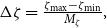 $\Delta \zeta =\frac {\zeta _{\max}-\zeta _{\min}}{M_{\zeta }},$
where
$\Delta \zeta =\frac {\zeta _{\max}-\zeta _{\min}}{M_{\zeta }},$
where $\zeta \in \{t, S,r,\lambda ,N\}$
and
$\zeta \in \{t, S,r,\lambda ,N\}$
and $M_{\zeta }$
denotes a strictly positive integer that represents the number of steps in the grid for
$M_{\zeta }$
denotes a strictly positive integer that represents the number of steps in the grid for $\zeta .$
Furthermore, we denote the time-consistent option price at time
$\zeta .$
Furthermore, we denote the time-consistent option price at time $i \Delta t$
, for an underlying asset price of
$i \Delta t$
, for an underlying asset price of $j_{S} \Delta S$
, with a mortality intensity value of
$j_{S} \Delta S$
, with a mortality intensity value of $j_{\lambda } \Delta \lambda$
, an interest rate value of
$j_{\lambda } \Delta \lambda$
, an interest rate value of $(r_{\min}+j_{r} \Delta r),$
and a current count of surviving policyholders
$(r_{\min}+j_{r} \Delta r),$
and a current count of surviving policyholders $j_{N} \Delta N$
by
$j_{N} \Delta N$
by $\tilde {\pi }_{i,j_{S},j_{r},j_{\lambda }}^{j_{N}},$
where
$\tilde {\pi }_{i,j_{S},j_{r},j_{\lambda }}^{j_{N}},$
where $j_{\tilde {\zeta }} \in \{0,1,\ldots ,M_{\tilde {\zeta }}\}$
for
$j_{\tilde {\zeta }} \in \{0,1,\ldots ,M_{\tilde {\zeta }}\}$
for $\tilde {\zeta }\in \{S,r,\lambda ,N\}$
and
$\tilde {\zeta }\in \{S,r,\lambda ,N\}$
and $i \in \{0,1,\ldots ,M_{t}\}.$
Given that the risk factors $\tilde {M_t}^{(1)}=\frac {N_t}{N_{t- t^{(1)}}}$
and
$\tilde {M_t}^{(1)}=\frac {N_t}{N_{t- t^{(1)}}}$
and $\tilde {M_t}^{(2)}=e^{-\int _{t- t^{(1)}}^t \lambda _s\textrm {d}s}$
are not Markovian processes,Footnote 15 we establish the terminal condition at the instant
$\tilde {M_t}^{(2)}=e^{-\int _{t- t^{(1)}}^t \lambda _s\textrm {d}s}$
are not Markovian processes,Footnote 15 we establish the terminal condition at the instant $T-t^{(1)}$
instead of at
$T-t^{(1)}$
instead of at $T$
. The definitive formula below follows from the closed-form expression in (26), the valuation of the call option under stochastic interest rates, and the log-normal distribution of the investment fund under
$T$
. The definitive formula below follows from the closed-form expression in (26), the valuation of the call option under stochastic interest rates, and the log-normal distribution of the investment fund under $\mathbb{P}^f$
 \begin{align*} \tilde {\pi }_{T-t^{(1)}}^{3}[{}_{T-t^{(1)}}H_{T}] &=C\times \big(P\big(T-t^{(1)},T\big)+\beta \big(S_{T-t^{(1)}}\Phi \big(d_{T-t^{(1)}}\big)-P\big(T-t^{(1)},T\big)PG \\ &\quad \times \Phi \big(d_{T- t^{(1)}}-n\big(T-t^{(1)},T\big)\big)\big) \big ) \times e^{-\lambda _{T-t^{(1)}}l_{T-t^{(1)},T}+\frac {1}{2}s_{T-t^{(1)},T}^2} \\ &\quad \times e^{-\theta _{T-t^{(1)},T}^{(1)} s_{T-t^{(1)},T}^2}+C \times \alpha _{T-t^{(1)}}\sqrt {t^{(1)}}P\big(T-t^{(1)},T\big)\Big [1+2\beta \big(S_{T-t^{(1)}} \\ & \quad \times e^{\mu _{S} t^{(1)}}\Phi (\delta _{T-t^{(1)}})-PG\Phi \big(\delta _{T-t^{(1)}}-\sigma _{S}\sqrt {t^{(1)}}\big)\big)+\beta ^{2}\Big (S_{T- t^{(1)}}^{2}e^{2\big(\mu _{S}+\frac {1}{2}\sigma _{S}^2\big)t^{(1)}} \\ & \quad \times \Phi \big(\delta _{T-t^{(1)}}+\sigma _{S}\sqrt {t^{(1)}}\big) +(PG)^{2}\Phi \big(\delta _{T- t^{(1)}}-\sigma _{S}\sqrt {t^{(1)}}\big)-2PGS_{T-t^{(1)}}e^{\mu_{S} t^{(1)}} \\ & \quad \times \Phi \big(\delta _{T-t^{(1)}}\big)\Big)\Big ]^{\frac {1}{2}} \times {\unicode {x1D7D9}_{N_{T-t^{(1)}}\gt 0}} \\ & \quad \times \sqrt {\frac {1}{N_{T-t^{(1)}}}\Big(e^{-\lambda _{T-t^{(1)}}l_{T-t^{(1)},T}+\frac {1}{2}s_{T- t^{(1)},T}^2} -e^{-2\lambda _{T-t^{(1)}}l_{T-t^{(1)},T}+2s_{T-t^{(1)},T}^2}\Big)}, \end{align*}
where
 \begin{align*} \delta _{T-t^{(1)}}&=\frac {\left(\mu _{S}+\frac {1}{2}\sigma _{S}^{2}\right)t^{(1)}+ln\left(\frac {S_{T-t^{(1)}}}{PG}\right)}{\sigma _{S}\sqrt {t^{(1)}}},\\ \theta _{T-t^{(1)},T}^{(1)}&=\frac {-0.16}{s_{T-t^{(1)},T}},\\ d_{T-t^{(1)}}&=\frac {\frac {1}{2}n\big(T-t^{(1)},T\big)^2+ln\left(\frac {S_{T-t^{(1)}}}{PG}\right)-ln\left(P\big(T-t^{(1)},T\big)\right)}{n\big(T-t^{(1)},T\big)},\\ n\big(T-t^{(1)},T\big)^2&=\sigma _S^2t^{(1)}+\frac {\sigma _r^2}{a^2}t^{(1)}+\frac {\sigma _r^2}{a^3}\left(\frac {-3}{2}-\frac {1}{2}e^{-2at^{(1)}}+2e^{-at^{(1)}}\right)+\frac {2\rho \sigma _S\sigma _r t^{(1)}}{a} \\ &\quad -\frac {2\rho \sigma _S\sigma _r\big(1-e^{-at^{(1)}}\big)}{a^2}. \end{align*}
The approximations for the partial derivatives existing in Theorem1 are detailed as follows
 \begin{equation*} \partial _{t} \tilde {\pi }_{i,j_{S},j_{r},j_{\lambda }}^{j_{N}} = \dfrac {\tilde {\pi }_{i+1,j_{S},j_{r},j_{\lambda }}^{j_{N}} - \tilde {\pi }_{i,j_{S},j_{r},j_{\lambda }}^{j_{N}}}{\Delta t},\ i\lt M_{t} \end{equation*}
 \begin{equation*} \partial _{S}\tilde {\pi }_{i,j_{S},j_{r},j_{\lambda }}^{j_{N}} = \begin{cases} \dfrac {\tilde {\pi }_{i+1,j_{S},j_{r},j_{\lambda }}^{j_{N}} - \tilde {\pi }_{i+1,j_{S}-2,j_{r},j_{\lambda }}^{j_{N}}}{2\Delta S} & \text{if } j_{S}=M_{S} \\[1em] \dfrac {\tilde {\pi }_{i+1,j_{S}+2,j_{r},j_{\lambda }}^{j_{N}} - \tilde {\pi }_{i+1,j_{S},j_{r},j_{\lambda }}^{j_{N}}}{2\Delta S} & \text{if } j_{S}=0 \\[1em] \dfrac {\tilde {\pi }_{i+1,j_{S}+1,j_{r},j_{\lambda }}^{j_{N}} - \tilde {\pi }_{i+1,j_{S}-1,j_{r},j_{\lambda }}^{j_{N}}}{2\Delta S} & \text{else} \end{cases} \end{equation*}
 \begin{equation*} \partial _{r}\tilde {\pi }_{i,j_{S},j_{r},j_{\lambda }}^{j_{N}} = \begin{cases} \dfrac {\tilde {\pi }_{i+1,j_{S},j_{r},j_{\lambda }}^{j_{N}} - \tilde {\pi }_{i+1,j_{S},j_{r}-2,j_{\lambda }}^{j_{N}}}{2\Delta r} & \text{if } j_{r}=M_{r} \\[1em] \dfrac {\tilde {\pi }_{i+1,j_{S},j_{r}+2,j_{\lambda }}^{j_{N}} - \tilde {\pi }_{i+1,j_{S},j_{r},j_{\lambda }}^{j_{N}}}{2\Delta r} & \text{if } j_{r}=0 \\[1em] \dfrac {\tilde {\pi }_{i+1,j_{S},j_{r}+1,j_{\lambda }}^{j_{N}} - \tilde {\pi }_{i+1,j_{S},j_{r}-1,j_{\lambda }}^{j_{N}}}{2\Delta r} & \text{else} \end{cases} \end{equation*}
 \begin{equation*} \partial _{\lambda }\tilde {\pi }_{i,j_{S},j_{r},j_{\lambda }}^{j_{N}} = \begin{cases} \dfrac {\tilde {\pi }_{i+1,j_{S},j_{r},j_{\lambda }}^{j_{N}} - \tilde {\pi }_{i+1,j_{S},j_{r},j_{\lambda }-2}^{j_{N}}}{2\Delta \lambda } & \text{if } j_{\lambda }=M_{\lambda } \\[1em] \dfrac {\tilde {\pi }_{i+1,j_{S},j_{r},j_{\lambda }+2}^{j_{N}} - \tilde {\pi }_{i+1,j_{S},j_{r},j_{\lambda }}^{j_{N}}}{2\Delta \lambda } & \text{if } j_{\lambda }=0 \\[1em] \dfrac {\tilde {\pi }_{i+1,j_{S},j_{r},j_{\lambda }+1}^{j_{N}} - \tilde {\pi }_{i+1,j_{S},j_{r},j_{\lambda }-1}^{j_{N}}}{2\Delta \lambda } & \text{else} \end{cases} \end{equation*}
 \begin{equation*} \partial _{S}^{2}\tilde {\pi }_{i,j_{S},j_{r},j_{\lambda }}^{j_{N}} = \begin{cases} \dfrac {\tilde {\pi }_{i+1,j_{S},j_{r},j_{\lambda }}^{j_{N}} -2\tilde {\pi }_{i+1,j_{S}-1,j_{r},j_{\lambda }}^{j_{N}} + \tilde {\pi }_{i+1,j_{S}-2,j_{r},j_{\lambda }}^{j_{N}}}{\Delta S^2} & \text{if } j_{S}=M_{S} \\[1em] \dfrac {\tilde {\pi }_{i+1,j_{S}+2,j_{r},j_{\lambda }}^{j_{N}} -2\tilde {\pi }_{i+1,j_{S}+1,j_{r},j_{\lambda }}^{j_{N}} + \tilde {\pi }_{i+1,j_{S},j_{r},j_{\lambda }}^{j_{N}}}{\Delta S^2}, & \text{if } j_{S}=0 \\[1em] \dfrac {\tilde {\pi }_{i+1,j_{S}+1,j_{r},j_{\lambda }}^{j_{N}} -2\tilde {\pi }_{i+1,j_{S},j_{r},j_{\lambda }}^{j_{N}} + \tilde {\pi }_{i+1,j_{S}-1,j_{r},j_{\lambda }}^{j_{N}}}{\Delta S^2} & \text{else} \end{cases} \end{equation*}
 \begin{align*} \partial _{r}^{2}\tilde {\pi }_{i,j_{S},j_{r},j_{\lambda }}^{j_{N}}=\left \{ \begin{array}{ll} \dfrac {\tilde {\pi }_{i+1,j_{S},j_{r},j_{\lambda }}^{j_{N}} -2\tilde {\pi }_{i+1,j_{S},j_{r}-1,j_{\lambda }}^{j_{N}} + \tilde {\pi }_{i+1,j_{S},j_{r}-2,j_{\lambda }}^{j_{N}}}{\Delta r^2 } \ \ \ \ \ \text{if } j_{r}=M_{r} \\[1em] \dfrac {\tilde {\pi }_{i+1,j_{S},j_{r}+2,j_{\lambda }}^{j_{N}} -2\tilde {\pi }_{i+1,j_{S},j_{r}+1,j_{\lambda }}^{j_{N}} + \tilde {\pi }_{i+1,j_{S},j_{r},j_{\lambda }}^{j_{N}}}{\Delta r^2} \ \ \ \ \ \text{if } j_{r}=0\\[1em] \dfrac {\tilde {\pi }_{i+1,j_{S},j_{r}+1,j_{\lambda }}^{j_{N}} -2\tilde {\pi }_{i+1,j_{S},j_{r},j_{\lambda }}^{j_{N}} + \tilde {\pi }_{i+1,j_{S},j_{r}-1,j_{\lambda }}^{j_{N}}}{\Delta r^{2} } \ \ \ \ \text{else} \\ \end{array} \right \} \end{align*}
 \begin{align*} \partial _{\lambda }^{2}\tilde {\pi }_{i,j_{S},j_{r},j_{\lambda }}^{j_{N}}=\left \{ \begin{array}{ll} \dfrac {\tilde {\pi }_{i+1,j_{S},j_{r},j_{\lambda }}^{j_{N}} -2\tilde {\pi }_{i+1,j_{S},j_{r},j_{\lambda }-1}^{j_{N}} + \tilde {\pi }_{i+1,j_{S},j_{r},j_{\lambda }-2}^{j_{N}}}{\Delta \lambda ^2 } \ \ \ \ \ \text{if } j_{\lambda }=M_{\lambda } \\[1em] \dfrac {\tilde {\pi }_{i+1,j_{S},j_{r},j_{\lambda }+2}^{j_{N}} -2\tilde {\pi }_{i+1,j_{S},j_{r},j_{\lambda }+1}^{j_{N}} + \tilde {\pi }_{i+1,j_{ S},j_{r},j_{\lambda }}^{j_{N}}}{\Delta \lambda ^2} \ \ \ \ \ \text{if } j_{\lambda }=0\\[1em] \dfrac {\tilde {\pi }_{i+1,j_{S},j_{r},j_{\lambda }+1}^{j_{N}} -2\tilde {\pi }_{i+1,j_{S},j_{r},j_{\lambda }}^{j_{N}} + \tilde {\pi }_{i+1,j_{S},j_{r},j_{\lambda }-1}^{j_{N}}}{\Delta \lambda ^{2} } \ \ \ \ \text{else}\\ \end{array} \right \} \end{align*}
 \begin{align*} (\tilde {\pi }^{*}-\tilde {\pi })_{i,j_{S},j_{r},j_{\lambda }}^{j_{N}}=\left \{ \begin{array}{ll} 0 \ \ \ \ \ \ \ \ \ \ \ \ \ \ \ \ \ \ \ \ \ \ \ \ \ \ \ \ \ \ \ \ \ \ \text{if } j_{N}=0 \\[6pt] \left(\tilde {\pi }_{i+1,j_{S},j_{r},j_{\lambda }}^{j_{N}-1}-\tilde {\pi }_{i+1,j_{S},j_{r},j_{\lambda }}^{j_{N}}\right) \ \ \text{else} \end{array} \right \} \end{align*}
 \begin{equation*} \partial _{rS}^{2}\tilde {\pi }_{i,j_{S},j_{r},j_{\lambda }}^{j_{N}} = \begin{cases} \dfrac {\substack {\tilde {\pi }_{i+1,j_{S},j_{r},j_{\lambda }}^{j_{N}} - \tilde {\pi }_{i+1,j_{S},j_{r}-2,j_{\lambda }}^{j_{N}}\\ \qquad \;+\; \tilde {\pi }_{i+1,j_{S}-2,j_{r}-2,j_{\lambda }}^{j_{N}} - \tilde {\pi }_{i+1,j_{S}-2,j_{r},j_{\lambda }}^{j_{N}}}} {4 \Delta S \Delta r} & \text{if } j_{S}=M_{S} \ \& \ j_{r}=M_{r} \\[1.2em] \dfrac {\substack {\tilde {\pi }_{i+1,j_{S},j_{r}+1,j_{\lambda }}^{j_{N}} - \tilde {\pi }_{i+1,j_{S},j_{r}-1,j_{\lambda }}^{j_{N}}\\\quad \;+\; \tilde {\pi }_{i+1,j_{S}-2,j_{r}-1,j_{\lambda }}^{j_{N}} - \tilde {\pi }_{i+1,j_{S}-2,j_{r}+1,j_{\lambda }}^{j_{N}}}} {4 \Delta S \Delta r} & \text{if } j_{S}=M_{S} \ \& \ j_{r}\ne M_{r},0 \\[1.2em] \dfrac {\substack {\tilde {\pi }_{i+1,j_{S}+1,j_{r},j_{\lambda }}^{j_{N}} - \tilde {\pi }_{i+1,j_{S}+1,j_{r}-2,j_{\lambda }}^{j_{N}}\\ \quad \;+\; \tilde {\pi }_{i+1,j_{S}-1,j_{r}-2,j_{\lambda }}^{j_{N}} - \tilde {\pi }_{i+1,j_{S}-1,j_{r},j_{\lambda }}^{j_{N}}}} {4 \Delta S \Delta r} & \text{if } j_{S}\ne M_{S},0 \ \& \ j_{r}=M_{r} \\[1.2em] \dfrac {\substack {\tilde {\pi }_{i+1,j_{S}+2,j_{r},j_{\lambda }}^{j_{N}} - \tilde {\pi }_{i+1,j_{S}+2,j_{r}-2,j_{\lambda }}^{j_{N}}\\ \quad \;+\; \tilde {\pi }_{i+1,j_{S},j_{r}-2,j_{\lambda }}^{j_{N}} - \tilde {\pi }_{i+1,j_{S},j_{r},j_{\lambda }}^{j_{N}}}} {4 \Delta S \Delta r} & \text{if } j_{S}=0 \ \& \ j_{r}=M_{r} \\[1.2em] \dfrac {\substack {\tilde {\pi }_{i+1,j_{S},j_{r}+2,j_{\lambda }}^{j_{N}} - \tilde {\pi }_{i+1,j_{S},j_{r},j_{\lambda }}^{j_{N}}\\ \quad \;+\; \tilde {\pi }_{i+1,j_{S}-2,j_{r},j_{\lambda }}^{j_{N}} - \tilde {\pi }_{i+1,j_{S}-2,j_{r}+2,j_{\lambda }}^{j_{N}}}} {4 \Delta S \Delta r} & \text{if } j_{S}=M_{S} \ \& \ j_{r}=0 \\[1.2em] \dfrac {\substack {\tilde {\pi }_{i+1,j_{S}+2,j_{r}+2,j_{\lambda }}^{j_{N}} - \tilde {\pi }_{i+1,j_{S}+2,j_{r},j_{\lambda }}^{j_{N}}\\ \quad \;+\; \tilde {\pi }_{i+1,j_{S},j_{r},j_{\lambda }}^{j_{N}} - \tilde {\pi }_{i+1,j_{S},j_{r}+2,j_{\lambda }}^{j_{N}}}} {4 \Delta S \Delta r} & \text{if } j_{S}=0 \ \& \ j_{r}=0 \\[1.2em] \dfrac {\substack {\tilde {\pi }_{i+1,j_{S}+2,j_{r}+1,j_{\lambda }}^{j_{N}} - \tilde {\pi }_{i+1,j_{S}+2,j_{r}-1,j_{\lambda }}^{j_{N}}\\ \quad \;+\; \tilde {\pi }_{i+1,j_{S},j_{r}-1,j_{\lambda }}^{j_{N}} - \tilde {\pi }_{i+1,j_{S},j_{r}+1,j_{\lambda }}^{j_{N}}}} {4 \Delta S \Delta r} & \text{if } j_{S}=0 \ \& \ j_{r}\ne 0,M_{r} \\[1.2em] \dfrac {\substack {\tilde {\pi }_{i+1,j_{S}+1,j_{r}+2,j_{\lambda }}^{j_{N}} - \tilde {\pi }_{i+1,j_{S}+1,j_{r},j_{\lambda }}^{j_{N}}\\ \quad \;+\; \tilde {\pi }_{i+1,j_{S}-1,j_{r},j_{\lambda }}^{j_{N}} - \tilde {\pi }_{i+1,j_{S}-1,j_{r}+2,j_{\lambda }}^{j_{N}}}} {4 \Delta S \Delta r} & \text{if } j_{S}\ne 0,M_{S} \ \& \ j_{r}=0 \\[1.2em] \dfrac {\substack {\tilde {\pi }_{i+1,j_{S}+1,j_{r}+1,j_{\lambda }}^{j_{N}} - \tilde {\pi }_{i+1,j_{S}+1,j_{r}-1,j_{\lambda }}^{j_{N}}\\ \quad \;+\; \tilde {\pi }_{i+1,j_{S}-1,j_{r}-1,j_{\lambda }}^{j_{N}} - \tilde {\pi }_{i+1,j_{S}-1,j_{r}+1,j_{\lambda }}^{j_{N}}}} {4 \Delta S \Delta r} & \text{else} \end{cases} \end{equation*}
Excluding the boundary conditions, the backward recursive scheme assumes the ensuing structure for $i \in \{0,1,\ldots ,M_{t}-1\}$
 \begin{align*} \tilde {\pi }_{i,j_{S},j_{r},j_{\lambda }}^{j_{N}} &=b_{j_{S},j_{r}}\tilde {\pi }_{i+1,j_{S},j_{r},j_{\lambda }}^{j_{N}}+c_{j_{S},j_{r}}^{+}\tilde {\pi }_{i+1,j_{S}+1,j_{r},j_{\lambda }}^{j_{N}}-c_{j_{S},j_{r}}^{-}\tilde {\pi }_{i+1,j_{S}-1,j_{r},j_{\lambda }}^{j_{N}}+d_{j_{r}}^{+}\tilde {\pi }_{i+1,j_{S},j_{r}+1,j_{\lambda }}^{j_{N}}\\&\quad -d_{j_{r}}^{-}\tilde {\pi }_{i+1,j_{S},j_{r}-1,j_{\lambda }}^{j_{N}}+\left(\overline {\theta _{i \Delta t,T-t^{(1)}}^{(1)}}\frac {g_{j_r}}{2\Delta \lambda }+e_{j_{r},j_{\lambda }}^{+}\right)\tilde {\pi }_{i+1,j_{S},j_{r},j_{\lambda }+1}^{j_{N}}- \left(\overline {\theta _{i \Delta t,T-t^{(1)}}^{(1)}}\frac {g_{j_r}}{2\Delta \lambda }+e_{j_{r},j_{\lambda }}^{-}\right) \\&\quad \times\tilde {\pi }_{i+1,j_{S},j_{r},j_{\lambda }-1}^{j_{N}}+ g_{j_{r}}P_{i+1,j_{S},j_{r},j_{\lambda }}^{j_{N}}+g_{j_{r}}\left(\tilde {\pi }_{i+1,j_{S},j_{r},j_{\lambda }}^{j_{N}-1}-\tilde {\pi }_{i+1,j_{S},j_{r},j_{\lambda }}^{j_{N}}\right)j_{\lambda } \Delta \lambda \\&\quad +\alpha _{i \Delta t}g_{j_{r}}\sqrt {S_{i+1,j_{S},j_{r},j_{\lambda }}^{j_{N}}+\left(\tilde {\pi }_{i+1,j_{S},j_{r},j_{\lambda }}^{j_{N}-1}-\tilde {\pi }_{i+1,j_{S},j_{r},j_{\lambda }}^{j_{N}}\right)^{2}j_{\lambda }\Delta \lambda }. \end{align*}
where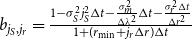 $b_{j_{S},j_{r}}=\frac {1-\sigma _{S}^{2}j_{S}^{2}\Delta t -\frac {\sigma _{m}^2}{\Delta \lambda ^2}\Delta t-\frac {\sigma _{r}^{2}\Delta t}{\Delta r ^2}}{1+(r_{\min}+j_{r}\Delta r) \Delta t}$
,
$b_{j_{S},j_{r}}=\frac {1-\sigma _{S}^{2}j_{S}^{2}\Delta t -\frac {\sigma _{m}^2}{\Delta \lambda ^2}\Delta t-\frac {\sigma _{r}^{2}\Delta t}{\Delta r ^2}}{1+(r_{\min}+j_{r}\Delta r) \Delta t}$
, $c_{j_{S},j_{r}}^{+-}=\frac {\frac {1}{2}(r_{\min}+j_{r}\Delta r)j_{S} \Delta t+-\frac {1}{2}\sigma _{S}^2j_{S}^2\Delta t }{1+(r_{\min}+j_{r}\Delta r) \Delta t},$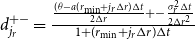 $d_{j_r}^{+-}=\frac {\frac {(\theta -a(r_{\min}+j_r\Delta r)\Delta t}{2\Delta r} +-\frac {\sigma _{r}^2\Delta t}{2\Delta r ^2}}{1+(r_{\min}+j_{r}\Delta r) \Delta t}$
,
$d_{j_r}^{+-}=\frac {\frac {(\theta -a(r_{\min}+j_r\Delta r)\Delta t}{2\Delta r} +-\frac {\sigma _{r}^2\Delta t}{2\Delta r ^2}}{1+(r_{\min}+j_{r}\Delta r) \Delta t}$
,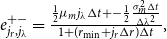 $e_{j_r,j_\lambda }^{+-}=\frac {\frac {1}{2}\mu _m j_{\lambda }\Delta t+-\frac {1}{2}\frac {\sigma _{m}^2\Delta t}{\Delta \lambda ^2}}{1+(r_{\min}+j_{r}\Delta r) \Delta t},$ $g_{j_r}=\frac {\Delta t }{1+(r_{\min}+j_{r}\Delta r) \Delta t},$ $P_{i+1,j_{S},j_{r},j_{\lambda }}^{j_N}=\rho \sigma _{r}\sigma _{S}j_{S} \frac {\tilde {\pi }_{i+1,j_{S}+1,j_{r}+1,j_{\lambda }}^{j_{N}} -\tilde {\pi }_{i+1,j_{S}+1,j_{r}-1,j_{\lambda }}^{j_{N}} +\tilde {\pi }_{i+1,j_{S}-1,j_{r}-1,j_{\lambda }}^{j_{N}}-\tilde {\pi }_{i+1,j_{S}-1,j_{r}+1,j_{\lambda }}^{j_{N}} }{4\Delta r}$
and
$P_{i+1,j_{S},j_{r},j_{\lambda }}^{j_N}=\rho \sigma _{r}\sigma _{S}j_{S} \frac {\tilde {\pi }_{i+1,j_{S}+1,j_{r}+1,j_{\lambda }}^{j_{N}} -\tilde {\pi }_{i+1,j_{S}+1,j_{r}-1,j_{\lambda }}^{j_{N}} +\tilde {\pi }_{i+1,j_{S}-1,j_{r}-1,j_{\lambda }}^{j_{N}}-\tilde {\pi }_{i+1,j_{S}-1,j_{r}+1,j_{\lambda }}^{j_{N}} }{4\Delta r}$
and $S_{i+1,j_{S},j_{r},j_{\lambda }}^{j_N}=(\sigma _{S}j_{S})^{2}\frac {\big(\tilde {\pi }_{i+1,j_{S}+1,j_{r},j_{\lambda }}^{j_{N}}-\tilde {\pi }_{i+1,j_{S}-1,j_{r},j_{\lambda }}^{j_{N}}\big)^{2}}{4}+\sigma _{m}^{2}\frac {\big(\tilde {\pi }_{i+1,j_{S},j_{r},j_{\lambda }+1}^{j_{N}}-\tilde {\pi }_{i+1,j_{S},j_{r},j_{\lambda }-1}^{j_{N}}\big)^{2}}{4\Delta \lambda ^2}+\sigma _{r}^{2}\frac {\big(\tilde {\pi }_{i+1,j_{S},j_{r}+1,j_{\lambda }}^{j_{N}}-\tilde {\pi }_{i+1,j_{S},j_{r}-1,j_{\lambda }}^{j_{N}}\big)^{2}}{4\Delta r^2}+\rho \sigma _{r} \sigma _{S}j_{S}\frac {\tilde {\pi }_{i+1,j_{S},j_{r}+1,j_{\lambda }}^{j_{N}} -\tilde {\pi }_{i+1,j_{S},j_{r}-1,j_{\lambda }}^{j_{N}}}{2\Delta r}\big(\tilde {\pi }_{i+1,j_{S}+1,j_{r},j_{\lambda }}^{j_{N}} -\tilde {\pi }_{i+1,j_{S}-1,j_{r},j_{\lambda }}^{j_{N}}\big).$
It is important to note that enforcing time consistency through the backward-iterative scheme defined in (23) does not require the same risk measure operator to be applied at every iteration. Hence, the $\alpha _{i\Delta t}$
-loading parameter of this backward algorithm does not need to remain identical across periods and can be recalibrated over time between periods.
$\alpha _{i\Delta t}$
-loading parameter of this backward algorithm does not need to remain identical across periods and can be recalibrated over time between periods.
4.3 Numerical results
We consider a cohort of $n=100$
females aged
$n=100$
females aged $35$
contracting a Pure Endowment with a terminal bonus. Our numerical application follows the assumptions used in Belhouari et al. (Reference Belhouari, Deelstra and Devolder2025), where the parameters characterizing our financial-actuarial models can be summarized as follows (see Table 1).
$35$
contracting a Pure Endowment with a terminal bonus. Our numerical application follows the assumptions used in Belhouari et al. (Reference Belhouari, Deelstra and Devolder2025), where the parameters characterizing our financial-actuarial models can be summarized as follows (see Table 1).
Numerical inputs
| Parameters | Numerical Values | $\alpha _t$
| $15\%$
| $i$
$i$
| $0.9\%$
| $C$
$C$
| $100,000$
| $T$
$T$
| $10$
$10$
| $P$
$P$
| $0.9070291$
| $r_{0}$
| $1.6$
%
$1.6$
% | $a$
$a$
| $40\%$
| $\theta$
| $0.8\%$
| $\sigma _r$
| $0.5\%$
| $\sigma _S$
| $15\%$
| $\rho$
| $20\%$
| $\mu _{S}$
| $5\%$
$5\%$
| $\beta$
| $40.19\%$
| $\lambda _0$
| $0.001080584$
| $\mu _m$
| $0.0745323698$
| $\sigma _m$
| $0.0002248628$
|

The Three-step method time-consistent dynamic with $M_S=35$
,
$M_S=35$
, $M_r=40$
,
$M_r=40$
, $M_{\lambda }=40$
,
$M_{\lambda }=40$
, $M_{N}=n=100$
, and,
$M_{N}=n=100$
, and, $S_t=S_{0},$ $r_t=r_{0}$
,
$r_t=r_{0}$
, $\lambda _t=\lambda _{0}$
,
$\lambda _t=\lambda _{0}$
, $N_{t}=n.$
(
$N_{t}=n.$
( $t^{(1)}=1$
).
$t^{(1)}=1$
).

The Three-step method time-consistent dynamic with $M_t=989$
,
$M_t=989$
, $M_S=35$
,
$M_S=35$
, $M_{\lambda }=40$
,
$M_{\lambda }=40$
, $M_{N}=n=100$
, and,
$M_{N}=n=100$
, and, $S_t=S_{0},$ $r_t=r_{0}$
,
$r_t=r_{0}$
, $\lambda _t=\lambda _{0}$
,
$\lambda _t=\lambda _{0}$
, $N_{t}=n.$
(
$N_{t}=n.$
( $t^{(1)}=1$
).
$t^{(1)}=1$
).
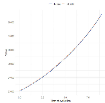
The Three-step method time-consistent dynamic with $M_t=989$
,
$M_t=989$
, $M_S=35$
,
$M_S=35$
, $M_r=40$
,
$M_r=40$
, $M_{N}=n=100,$
and,
$M_{N}=n=100,$
and, $S_t=S_{0},$ $r_t=r_{0}$
,
$r_t=r_{0}$
, $\lambda _t=\lambda _{0}$
,
$\lambda _t=\lambda _{0}$
, $N_{t}=n.$
(
$N_{t}=n.$
( $t^{(1)}=1$
).
$t^{(1)}=1$
).

The three-step method time-consistent dynamic with $M_t=989$
,
$M_t=989$
, $M_{\lambda }=40,$ $M_r=40$
,
$M_r=40$
, $M_{N}=n=100,$
and,
$M_{N}=n=100,$
and, $S_t=S_{0},$ $r_t=r_{0}$
,
$r_t=r_{0}$
, $\lambda _t=\lambda _{0}$
,
$\lambda _t=\lambda _{0}$
, $N_{t}=n.$
(
$N_{t}=n.$
( $t^{(1)}=1$
).
$t^{(1)}=1$
).

The dynamic Three-step method in the static versus time-consistent case and the best estimate under $\mathbb{Z}_{\theta }^{a}\times \mathbb{Q}^{\,f}$
. (
$\mathbb{Z}_{\theta }^{a}\times \mathbb{Q}^{\,f}$
. ( $t^{(1)}=1$
).
$t^{(1)}=1$
).

The dynamic Three-step method net of the best estimate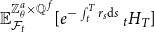 $\mathbb{E}_{\mathcal{F}_{t}}^{\mathbb{Z}_{\theta }^{a}\times \mathbb{Q}^{\,f}}[e^{-\int _{t}^T r_s\textrm {d}s}\ _{t}H_{T}]$
in the static versus time-consistent cases. (
$\mathbb{E}_{\mathcal{F}_{t}}^{\mathbb{Z}_{\theta }^{a}\times \mathbb{Q}^{\,f}}[e^{-\int _{t}^T r_s\textrm {d}s}\ _{t}H_{T}]$
in the static versus time-consistent cases. ( $t^{(1)}=1$
).
$t^{(1)}=1$
).

Prior to elucidating the numerical results, we must preliminarily verify the convergence of the finite difference method. Since the discretization step $\Delta N$
remains invariably equal to
$\Delta N$
remains invariably equal to $1$
,Footnote 16 it obviates the need for any calibration of the number of steps concerning the number of survivors. As depicted in Figure 1, the convergence of time is reached after
$1$
,Footnote 16 it obviates the need for any calibration of the number of steps concerning the number of survivors. As depicted in Figure 1, the convergence of time is reached after $989$
iterations, implying that approximately one iteration occurs every three days and one tier. Figures 2–4 respectively investigate the convergence of interest rates, mortality rates, and the financial investment fund. The stability of the numerical values is deemed sufficient for
$989$
iterations, implying that approximately one iteration occurs every three days and one tier. Figures 2–4 respectively investigate the convergence of interest rates, mortality rates, and the financial investment fund. The stability of the numerical values is deemed sufficient for $M_S=35$
,
$M_S=35$
, $M_r=40$
and
$M_r=40$
and $M_{\lambda }=40$
. Figure 5 contrasts the time-consistent values of the Three-step method with its static counterparts and the best estimate calculated under
$M_{\lambda }=40$
. Figure 5 contrasts the time-consistent values of the Three-step method with its static counterparts and the best estimate calculated under $\mathbb{Z}_{\theta }^{a}\times \mathbb{Q}^{\,f}$
. The dynamic Three-step method follows a monotonic trend analogous to that of the best estimate, reflecting a price upward over time. Furthermore, it demonstrates that the static values of the dynamic Three-step method exhibit a modest increase, ultimately resulting in a
$\mathbb{Z}_{\theta }^{a}\times \mathbb{Q}^{\,f}$
. The dynamic Three-step method follows a monotonic trend analogous to that of the best estimate, reflecting a price upward over time. Furthermore, it demonstrates that the static values of the dynamic Three-step method exhibit a modest increase, ultimately resulting in a $3.7\%$
cumulative growth by time
$3.7\%$
cumulative growth by time $0$
. By including the diversifiable part, the dynamic Three-step method loses its time-consistent property, which it previously maintained with a valuation formula equivalent to
$0$
. By including the diversifiable part, the dynamic Three-step method loses its time-consistent property, which it previously maintained with a valuation formula equivalent to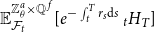 $\mathbb{E}_{\mathcal{F}_{t}}^{\mathbb{Z}_{\theta }^{a}\times \mathbb{Q}^{\,f}}[e^{-\int _{t}^T r_s\textrm {d}s}\ _{t}H_{T}]$
, as referenced in Lemma1. Therefore, to better understand the effect of time-consistency, it is important to compare the time-consistent Three-step prices, net of this best estimate, with the one-period Three-step prices, net again of this best estimate.Footnote 17 As we can see in Figure 6, the static values undergo a substantial increase, ending in an
$\mathbb{E}_{\mathcal{F}_{t}}^{\mathbb{Z}_{\theta }^{a}\times \mathbb{Q}^{\,f}}[e^{-\int _{t}^T r_s\textrm {d}s}\ _{t}H_{T}]$
, as referenced in Lemma1. Therefore, to better understand the effect of time-consistency, it is important to compare the time-consistent Three-step prices, net of this best estimate, with the one-period Three-step prices, net again of this best estimate.Footnote 17 As we can see in Figure 6, the static values undergo a substantial increase, ending in an $185\%$
increase by time
$185\%$
increase by time $0$
. To address this issue, we follow Devolder and Lebègue (Reference Devolder and Lebègue2016) and adjust the
$0$
. To address this issue, we follow Devolder and Lebègue (Reference Devolder and Lebègue2016) and adjust the $\alpha _{i \Delta t}$
safety loads portion applied in the backward recursive scheme. In our study, we propose a linear decrease of the safety loads portion over the entire time frame, within the backward algorithm,Footnote 18 as detailed below
$\alpha _{i \Delta t}$
safety loads portion applied in the backward recursive scheme. In our study, we propose a linear decrease of the safety loads portion over the entire time frame, within the backward algorithm,Footnote 18 as detailed below
 \begin{align*} \alpha _{i\Delta t} = \left \{ \begin{array}{ll} \dfrac {0.15}{989}\, i. & 0 \le i \le 989 \end{array} \right \}\!. \end{align*}
As illustrated in Figure 6, the linear recalibration of the safety loading portion successfully reduces the percentage increase induced by time consistency at time $0$
to a value below
$0$
to a value below $100\%$
, namely
$100\%$
, namely $23\%$
. Our decision to implement a backward-decreasing safety loading portion is primarily motivated by the objective of reducing the time-consistent price, which would otherwise have been prohibitively high. Moreover, this choice of a monotonically decreasing safety loading portion is also supported in the actuarial literature, see, for example, Hürlimann (Reference Hürlimann2010) and Devolder and Lebègue (Reference Devolder and Lebègue2016), where in the context of dynamic capital requirement calculation, the analog of the safety loading portion corresponds to the confidence level applied to Value-at-Risk. With this portion loading recalibration approach, we achieve a good compromise between a time-consistent evaluation methodology and a value that is not overly costly relative to the benchmark static value. This therefore proves that it is possible to switch to a time-consistent valuation without generating an unreasonable risk margin.
$23\%$
. Our decision to implement a backward-decreasing safety loading portion is primarily motivated by the objective of reducing the time-consistent price, which would otherwise have been prohibitively high. Moreover, this choice of a monotonically decreasing safety loading portion is also supported in the actuarial literature, see, for example, Hürlimann (Reference Hürlimann2010) and Devolder and Lebègue (Reference Devolder and Lebègue2016), where in the context of dynamic capital requirement calculation, the analog of the safety loading portion corresponds to the confidence level applied to Value-at-Risk. With this portion loading recalibration approach, we achieve a good compromise between a time-consistent evaluation methodology and a value that is not overly costly relative to the benchmark static value. This therefore proves that it is possible to switch to a time-consistent valuation without generating an unreasonable risk margin.
5. Conclusion
This paper explores the extension of the Three-step method to the dynamic context. To achieve this, we first refine the axiomatization of valuation operators, as well as the properties of market-consistency and actuarial-consistency, ultimately deriving a dynamic Three-step decomposition. We defined a crucial concept from the literature known as time-consistency. Furthermore, we presented an iterative backward procedure in a discrete model, enabling the enforcement of time-consistent dynamics where such consistency is previously absent. With a combination of any hybrid Pure Endowment product, we identified that the diversifiable component of the Three-step method detrimentally induces the non-verification of the time-consistent property. Therefore, we applied the backward procedure through a dual approach to the Three-step method to derive closed, time-consistent formulas using the purely actuarial Pure Endowment product. Thanks to the two-iteration closed-form solution, we observed that the diversifiable part influences the valuation of the non-diversifiable components of the subsequent iteration. Thus, achieving time-consistency by relying on traditional non-linear actuarial operators, such as the variance/standard-deviation premium principle, to assess the diversifiable part is not entirely viable. Immersed in the continuous-time limit, a PDE governing the Three-step method time-consistent dynamic was derived. By specifying a financial terminal bonus as the financial payoff of the hybrid life Pure Endowment product, the PDE was numerically solved using the finite difference method. The obtained numerical results indicated that the effect of time led to a slight rise in the one-step prices of the full Three-step method. Nonetheless, the static prices of the diversifiable actuarial component have surged notably when compared to the time-consistent Three-step prices, net of the best estimate under $\mathbb{Z}_{\theta }^{a} \times \mathbb{Q}^{\,f}$
. That being said, the time-consistent property, though essential for ensuring the consistency of the insurer’s internal decisions over time, is not immune to criticism and may have specific downsides. To mitigate the resulting impact, the safety charges applied in the backward scheme were progressively reduced through a linear approach. In most cases, the actuary managing liability assessments has considerable flexibility in setting the level of security measures to apply. When necessary, a more risk-averse strategy can be employed by increasing the security proportion loading, causing prices to increase. Conversely, a less cautious approach permits a reduction in the loading, resulting in lower prices. In our case, moderating the security loadings becomes a rational decision to ensure a suitable trade-off between time-consistency and the smooth progression of price changes. This indicates that careful consideration is required concerning the magnitude of security charges used in the backward scheme when applying non-linear actuarial premium principles to the valuation of the diversifiable part of the Three-step method.
$\mathbb{Z}_{\theta }^{a} \times \mathbb{Q}^{\,f}$
. That being said, the time-consistent property, though essential for ensuring the consistency of the insurer’s internal decisions over time, is not immune to criticism and may have specific downsides. To mitigate the resulting impact, the safety charges applied in the backward scheme were progressively reduced through a linear approach. In most cases, the actuary managing liability assessments has considerable flexibility in setting the level of security measures to apply. When necessary, a more risk-averse strategy can be employed by increasing the security proportion loading, causing prices to increase. Conversely, a less cautious approach permits a reduction in the loading, resulting in lower prices. In our case, moderating the security loadings becomes a rational decision to ensure a suitable trade-off between time-consistency and the smooth progression of price changes. This indicates that careful consideration is required concerning the magnitude of security charges used in the backward scheme when applying non-linear actuarial premium principles to the valuation of the diversifiable part of the Three-step method.
Data availability statement
This research did not use any data, hence data availability is not applicable.
Funding statement
This work received no specific grant from any funding agency, commercial or not-for-profit sectors.
Competing interests
No potential conflict of interest was reported by the authors.
Appendices
A. Asymptotic behavior of the standard deviation premium-variance principle
Details about
 \begin{align*} \pi _{t}^{u,SD}\big(_tH_u^{2} |\mathcal{F}_t\big)\underset {N_{t}\to +\infty }{\longrightarrow }0, \end{align*}
 \begin{align*} \pi _{t}^{u,V}\big(_tH_u^{2} |\mathcal{F}_t\big)\underset {N_{t}\to +\infty }{\longrightarrow }0, \end{align*}
for any $t\in [0,T].$
Proof.
Let $0\le t \le u\le T,$
such that
$0\le t \le u\le T,$
such that $N_t\gt 0.$
By construction, the actuarial component in
$N_t\gt 0.$
By construction, the actuarial component in $_tH_u^{2}$
involves a sum of actuarial risks centered under the real-world actuarial probability. Consequently, relying on the independence between financial and actuarial risks, the best estimate is immediately zero:
$_tH_u^{2}$
involves a sum of actuarial risks centered under the real-world actuarial probability. Consequently, relying on the independence between financial and actuarial risks, the best estimate is immediately zero:
 \begin{align*} \mathbb{E}_{\mathcal{F}_t}^{\mathbb{P}^a\times \mathbb{Q}^{\,f}}\big[e^{-\int _{t}^ur_s\textrm {d}s}\ _tH_u^{2} \big]=0.\end{align*}
Using the same argument of independence and centering, we obtain for the loading term
 \begin{align*} \mathbb{V}_{\mathcal{F}_t}\big[ _tH_u^{2}\big] &=\dfrac {1}{N_t^2}\mathbb{E}_{\mathcal{F}_t}[h(S_{u})^{2}]\times \mathbb{V}_{\mathcal{F}_t}\left[\sum _{j=1}^{N_t} (g(\tau _j)-\mathbb{E}_{\mathcal{F}_t\lor \mathfrak{S}_u}[g(\tau _j)] )\right]. \end{align*}
Applying the law of total variance to $\mathbb{V}_{\mathcal{F}_t}\big[\sum _{j=1}^{N_t}(g(\tau _j)-\mathbb{E}_{\mathcal{F}_t\lor \mathfrak{S}_u}[g(\tau _j)])\big]$
conditioned on
$\mathbb{V}_{\mathcal{F}_t}\big[\sum _{j=1}^{N_t}(g(\tau _j)-\mathbb{E}_{\mathcal{F}_t\lor \mathfrak{S}_u}[g(\tau _j)])\big]$
conditioned on $\mathfrak{S}_u \vee \mathcal{F}_t$
, and exploiting the i.i.d. property of remaining lifetimes conditional on
$\mathfrak{S}_u \vee \mathcal{F}_t$
, and exploiting the i.i.d. property of remaining lifetimes conditional on $\mathfrak{S}_u$
, we obtain:
$\mathfrak{S}_u$
, we obtain:
 \begin{align*} \mathbb{V}_{\mathcal{F}_t}\left[\sum _{j=1}^{N_t} (g(\tau _j)-\mathbb{E}_{\mathcal{F}_t\lor \mathfrak{S}_u}[g(\tau _j)] )\right] &=N_{t} \times \mathbb{E}_{\mathcal{F}_t} [\mathbb{V}_{\mathcal{F}_t\lor \mathfrak{S}_u} [g(\tau _1) ] ]. \end{align*}
Thus,
 \begin{align*} \mathbb{V}_{\mathcal{F}_t}[ _tH_u^{2}] &=\mathbb{E}_{\mathcal{F}_t}[h(S_{u})^{2}]\times \dfrac {1}{N_{t}}\times \mathbb{E}_{\mathcal{F}_t} [\mathbb{V}_{\mathcal{F}_t\lor \mathfrak{S}_u} [g(\tau _1) ] ]. \end{align*}
Finally
 \begin{align*} \left \{ \begin{array}{ll} \pi _t^{u,V}\big( _tH_u^{2} |\mathcal{F}_t\big)=\gamma _{t}\times \mathbb{E}_{\mathcal{F}_t}[h(S_u)^2] \times \frac {\mathbb{E}_{\mathcal{F}_t} [\mathbb{V}_{\mathcal{F}_t\lor \mathfrak{S}_u} [g(\tau _1) ] ]}{N_t} \times P(t,u).\\[9pt] \pi _t^{u,SD}\big( _tH_u^{2} |\mathcal{F}_t\big)=\alpha _{t}\times \sqrt {\mathbb{E}_{\mathcal{F}_t}[h(S_u)^2]}\times \sqrt {\frac { \mathbb{E}_{\mathcal{F}_t} [\mathbb{V}_{\mathcal{F}_t\lor \mathfrak{S}_u} [g(\tau _1) ] ]}{N_t}}\times \sqrt {u-t}\times P(t,u). \end{array} \right \}\!. \end{align*}
Therefore $\pi _{t}^{u,SD}(_tH_u^{2} |\mathcal{F}_t)\underset {N_{t}\to +\infty }{\longrightarrow }0,$
and
$\pi _{t}^{u,SD}(_tH_u^{2} |\mathcal{F}_t)\underset {N_{t}\to +\infty }{\longrightarrow }0,$
and $\pi _{t}^{u,V}(_tH_u^{2} |\mathcal{F}_t)\underset {N_{t}\to +\infty }{\longrightarrow }0.$
B. Equivalence of time-consistency definitions
Details about Remark 1.
Proof.
-
1. Time-consistent property
$\Rightarrow$
Iterated property: Let
$ 0\le t \le u\le T$
,
$ 0\lt s \le u-t$
and
$h \in \mathcal{H}_u^f.$
The translation invariance axiom implies that,Since
\begin{align*} \pi _{t+s}^{t+s} \big[\pi _{t+s}^{u} [h ] \big]=\pi _{t+s}^{u}[h]. \end{align*}
$\pi _{t+s}^{u}[h]\in \mathcal{H}_{t+s}^f,$
we can therefore apply (16) twice:
\begin{align*} \pi _{t+s}^{t+s} \big[\pi _{t+s}^{u} [h ] \big]\le \pi _{t+s}^{u}[h] \implies \pi _{t}^{t+s} \big[\pi _{t+s}^{u} [h ] \big]\le \pi _{t}^{u}[h]. \end{align*}
Hence, we reach the iterative definition.
\begin{align*} \pi _{t+s}^{t+s} \big[\pi _{t+s}^{u} [h ] \big]\ge \pi _{t+s}^{u}[h] \implies \pi _{t}^{t+s} \big[\pi _{t+s}^{u} [h ] \big]\ge \pi _{t}^{u}[h]. \end{align*}
-
2. Iterated property
$\Rightarrow$
Time-consistent property: Under the assumption of monotonicity, we embark on the verification of the converse direction. Let
$ 0\le t \le u,v\le T$
,
$ 0\lt s \le u-t$
,
$0\lt s \le v-t$
,
$h \in \mathcal{H}_u^f$
,
$g \in \mathcal{H}_v^f$
such as
$\pi _{t+s}^{u}[h]\le \pi _{t+s}^{v}[g]$
. Since
$\pi _{t+s}^{u}[h] \in \mathcal{H}_{t+s}^f$
,
$\pi _{t+s}^{v}[g] \in \mathcal{H}_{t+s}^f$
, then by monotonicityHence, using (17),
\begin{align*} \pi _{t}^{t+s} \big[\pi _{t+s}^{u} [h ] \big] \le \pi _{t}^{t+s} \big[\pi _{t+s}^{v} [g ] \big]. \end{align*}
\begin{align*} \pi _{t}^{u}[h]\le \pi _{t}^{v}[g]. \end{align*}


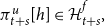






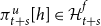
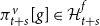


C. Time-inconsistency of the dynamic Three-step method: due to the diversifiable component
C.1 Details about Lemma1
Proof.
Intuition of why the Two-step method is time-consistent: The Two-step valuation is identified as a product of expectations under the risk-neutral probability $\mathbb{Q}^{\,f}$
and the actuarial probability
$\mathbb{Q}^{\,f}$
and the actuarial probability $\mathbb{Z}^a_\theta$
. Since expectations are linear and satisfy the tower rule property, the valuation operator satisfies time-consistency.
$\mathbb{Z}^a_\theta$
. Since expectations are linear and satisfy the tower rule property, the valuation operator satisfies time-consistency.
Let $0\le t \le u\le T$
such as
$0\le t \le u\le T$
such as $0\lt s\le u-t$
and
$0\lt s\le u-t$
and $N_{t+s}\gt 0$
. The one-period Two-step valuation at time
$N_{t+s}\gt 0$
. The one-period Two-step valuation at time $t+s$
with maturity
$t+s$
with maturity $u$
is given by
$u$
is given by
 \begin{align*} \pi _{t+s}^{u,2}[{}_{t+s}H_{u}]=\mathbb{E}_{\mathcal{F}_{t+s}}^{\mathbb{Q}^{\,f}}\big[e^{-\int _{t+s}^u r_v\textrm { d}v}h(S_u)\big]\times \mathbb{E}_{\mathcal{F}_{t+s}}^{\mathbb{Z}_{\theta }^{a}}\big[e^{-\int _{t+s}^u \lambda _v\textrm { d}v}\big]. \end{align*}
Let us set $_{t}LY_{t+s}=\frac {N_{t+s}}{N_t}\times \pi _{t+s}^{u,2}[{}_{t+s}H_{u}]=\mathbb{E}_{\mathcal{F}_{t+s}}^{\mathbb{Q}^{\,f}}[e^{-\int _{t+s}^u r_v\textrm { d}v}h(S_u)]\times \frac {N_{t+s}}{N_t}\times \mathbb{E}_{\mathcal{F}_{t+s}}^{\mathbb{Z}_{\theta }^{a}}[e^{-\int _{t+s}^u \lambda _v\textrm {d}v}],$
then its two-step decomposition is
$_{t}LY_{t+s}=\frac {N_{t+s}}{N_t}\times \pi _{t+s}^{u,2}[{}_{t+s}H_{u}]=\mathbb{E}_{\mathcal{F}_{t+s}}^{\mathbb{Q}^{\,f}}[e^{-\int _{t+s}^u r_v\textrm { d}v}h(S_u)]\times \frac {N_{t+s}}{N_t}\times \mathbb{E}_{\mathcal{F}_{t+s}}^{\mathbb{Z}_{\theta }^{a}}[e^{-\int _{t+s}^u \lambda _v\textrm {d}v}],$
then its two-step decomposition is
 \begin{align*} \left \{ \begin{array}{ll} _{t}LY_{t+s}^{h}=\mathbb{E}_{\mathcal{F}_{t}\lor \mathcal{F}_{t+s}^f}[{}_{t}LY_{t+s}]=\mathbb{E}_{\mathcal{F}_{t+s}}^{\mathbb{Q}^{\,f}}\big[e^{-\int _{t+s}^u r_v\textrm {d}v}h(S_u)\big]\times \mathbb{E}_{\mathcal{F}_{t}} \left[\mathbb{E}_{\mathcal{F}_{t+s}}^{\mathbb{Z}_{\theta }^{a}} \big[e^{-\int _{t}^u \lambda _v\textrm {d}v} \big] \right]\times {\unicode {x1D7D9}_{N_{t}\gt 0}},\\ _{t}LY_{t+s}^{sy}= \left({}_{t}LY_{t+s}-\mathbb{E}_{\mathcal{F}_{t+s}}^{\mathbb{Q}^{\,f}}\big[e^{-\int _{t+s}^u r_v\textrm { d}v}h(S_u)\big]\times \mathbb{E}_{\mathcal{F}_{t}} \left[\mathbb{E}_{\mathcal{F}_{t+s}}^{\mathbb{Z}_{\theta }^{a}} \big[e^{-\int _{t}^u \lambda _v\textrm {d}v} \big] \right] \right)\times {\unicode {x1D7D9}_{N_{t}\gt 0}}. \end{array} \right \} \end{align*}
The Two-step evaluation between times $t$
and
$t$
and $t+s$
is defined as follows
$t+s$
is defined as follows
 \begin{align*} \pi _{t}^{t+s,2}\left[\frac {N_{t+s}}{N_t}\times \pi _{t+s}^{u,2} [{}_{t+s}H_{u} ]\right]=\pi _{t}^{t+s,f}\big[{}_{t}LY_{t+s}^h\big]+\pi _{t}^{t+s,n}\big[{}_{t}LY_{t+s}^{sy}\big]. \end{align*}
Since the actuarial risks contained in the hedgeable part $_{t}LY_{t+s}^{h}$
are
$_{t}LY_{t+s}^{h}$
are $\mathcal{F}_{t}$
-measurable, its evaluation is identical in
$\mathcal{F}_{t}$
-measurable, its evaluation is identical in $\pi _{t}^{t+s,f}[{}_{t}LY_{t+s}^h]$
and in
$\pi _{t}^{t+s,f}[{}_{t}LY_{t+s}^h]$
and in $\pi _{t}^{t+s,n}[{}_{t}LY_{t+s}^{sy}]$
; the choice of probability measure (whether
$\pi _{t}^{t+s,n}[{}_{t}LY_{t+s}^{sy}]$
; the choice of probability measure (whether $\mathbb{Z}_{\theta }^{a}$
or
$\mathbb{Z}_{\theta }^{a}$
or $\mathbb{P}^a$
) has no effect. Hence, the valuation of the hedgeable component therefore cancels upon subtraction, and we obtain
$\mathbb{P}^a$
) has no effect. Hence, the valuation of the hedgeable component therefore cancels upon subtraction, and we obtain
 \begin{align*} \pi _{t}^{t+s,2}\left[\frac {N_{t+s}}{N_t}\times \pi _{t+s}^{u,2} [{}_{t+s}H_{u}]\right]=\mathbb{E}_{\mathcal{F}_{t}}^{\mathbb{Z}_{\theta }^{a} \times \mathbb{Q}^{\,f}}\big[e^{-\int _{t}^{t+s} r_v\textrm {d}v}\ _{t}LY_{t+s}\big]. \end{align*}
Using the independence between mortality and finance and tower rule property under $\mathbb{Z}_{\theta }^{a}$
and
$\mathbb{Z}_{\theta }^{a}$
and $\mathbb{Q}^{\,f}$
, we obtain
$\mathbb{Q}^{\,f}$
, we obtain
 \begin{align*} \pi _{t}^{t+s,2}\left[\frac {N_{t+s}}{N_t}\times \pi _{t+s}^{u,2} [{}_{t+s}H_{u} ]\right] &=\mathbb{E}_{\mathcal{F}_{t}}^{\mathbb{Q}^{\,f}}\big[e^{-\int _{t}^u r_v\textrm {d}v}h(S_u)\big]\times \mathbb{E}_{\mathcal{F}_{t}}^{\mathbb{Z}_{\theta }^{a}}\big[e^{-\int _{t}^u \lambda _v\textrm {d}v}\big]\\ &=\pi _{t}^{u,2}[{}_{t}H_{u}]. \end{align*}
Thus, the time-consistent valuation at time $t \in [0,T]$
can be calculated as
$t \in [0,T]$
can be calculated as $\pi _{t}^{2}[{}_{t}H_{T}]=\mathbb{E}_{\mathcal{F}_{t}}^{\mathbb{Q}^{\,f}}[e^{-\int _{t}^T r_v\textrm {d}v}h(S_T)]\times \mathbb{E}_{\mathcal{F}_{t}}^{\mathbb{Z}_{\theta }^{a}}[e^{-\int _{t}^T \lambda _v\textrm {d}v}].$
C.2 Details about Lemma2
Proof. Intuition: Unlike the Two-step method, which relies solely on linear expectations, the Three-step method assesses diversifiable risk using a variance (or standard deviation) premium principle. Variance is a non-linear operator that does not satisfy the tower rule property. This highlights that the iterative scheme fails to capture the variance of the conditional expectation component, producing the discrepancy between static and iterated valuations.
For the proof, we rely on the variance premium principle as the operator for evaluating the diversifiable risk. Notably, the result holds true under the standard deviation premium principle, and the proof can be readily adapted. Let $0\le t \le u\le T$
such as
$0\le t \le u\le T$
such as $0\lt s\le u-t$
and
$0\lt s\le u-t$
and $N_{t+s}\gt 0$
. The one-period Three-step valuation at time
$N_{t+s}\gt 0$
. The one-period Three-step valuation at time $t+s$
with maturity
$t+s$
with maturity $u$
is given by
$u$
is given by
 \begin{align} \pi _{t+s}^{u,3}[{}_{t+s}H_{u}] &=\mathbb{E}_{\mathcal{F}_{t+s}}^{\mathbb{Q}^{\,f}}\big[e^{-\int _{t+s}^u r_v\textrm {d}v}h(S_u)\big] \times \mathbb{E}_{\mathcal{F}_{t+s}}^{\mathbb{Z}_{\theta }^{a}}\big[e^{-\int _{t+s}^u \lambda _v\textrm {d}v}\big]+\gamma _{t+s} \times P(t+s,u) \notag \\ & \quad \times \frac {\mathbb{E}_{\mathcal{F}_{t+s}} \big[e^{-\int _{t+s}^u \lambda _v\textrm {d}v} \big(1-e^{-\int _{t+s}^u \lambda _v\textrm {d}v} \big) \big]}{N_{t+s}} \times \mathbb{E}_{\mathcal{F}_{t+s}}[h(S_u)^2]. \end{align}
Let us set $_{t}LY_{t+s}=\frac {N_{t+s}}{N_t}\times \pi _{t+s}^{u,3}[{}_{t+s}H_{u}]=\mathbb{E}_{\mathcal{F}_{t+s}}^{\mathbb{Q}^{\,f}}[e^{-\int _{t+s}^u r_v\textrm { d}v}h(S_u)]\frac {N_{t+s}}{N_t} \times \mathbb{E}_{\mathcal{F}_{t+s}}^{\mathbb{Z}_{\theta }^{a}}[e^{-\int _{t+s}^u \lambda _v\textrm {d}v}]+\gamma _{t+s} \times P(t+s,u) \ \times \frac {\mathbb{E}_{\mathcal{F}_{t+s}} [e^{-\int _{t+s}^u \lambda _v\textrm { d}v} (1-e^{-\int _{t+s}^u \lambda _v\textrm {d}v} ) ]}{N_{t}} \times \mathbb{E}_{\mathcal{F}_{t+s}}[h(S_u)^2],$
then its Three-step decomposition is
$_{t}LY_{t+s}=\frac {N_{t+s}}{N_t}\times \pi _{t+s}^{u,3}[{}_{t+s}H_{u}]=\mathbb{E}_{\mathcal{F}_{t+s}}^{\mathbb{Q}^{\,f}}[e^{-\int _{t+s}^u r_v\textrm { d}v}h(S_u)]\frac {N_{t+s}}{N_t} \times \mathbb{E}_{\mathcal{F}_{t+s}}^{\mathbb{Z}_{\theta }^{a}}[e^{-\int _{t+s}^u \lambda _v\textrm {d}v}]+\gamma _{t+s} \times P(t+s,u) \ \times \frac {\mathbb{E}_{\mathcal{F}_{t+s}} [e^{-\int _{t+s}^u \lambda _v\textrm { d}v} (1-e^{-\int _{t+s}^u \lambda _v\textrm {d}v} ) ]}{N_{t}} \times \mathbb{E}_{\mathcal{F}_{t+s}}[h(S_u)^2],$
then its Three-step decomposition is
 \begin{align*} \left \{ \begin{array}{ll} _{t}LY_{t+s}^{1}=\mathbb{E}_{\mathcal{F}_{t}\lor \mathcal{F}_{t+s}^f}[{}_{t}LY_{t+s}]= \left(\mathbb{E}_{\mathcal{F}_{t+s}}^{\mathbb{Q}^{\,f}}\big[e^{-\int _{t+s}^u r_v\textrm {d}v}h(S_u)\big]\times \mathbb{E}_{\mathcal{F}_{t}} \left[\mathbb{E}_{\mathcal{F}_{t+s}}^{\mathbb{Z}_{\theta }^{a}} \big[e^{-\int _{t}^u \lambda _v\textrm {d}v} \big] \right]\right.\\\left. +\gamma _{t+s} \times \dfrac {\mathbb{E}_{\mathcal{F}_{t}} \big[e^{-\int _{t+s}^u \lambda _v\textrm {d}v} \big(1-e^{-\int _{t+s}^u \lambda _v\textrm {d}v} \big) \big]}{N_{t}}\times \mathbb{E}_{\mathcal{F}_{t+s}}[h(S_u)^2]\times P(t+s,u) \right)\times {\unicode {x1D7D9}_{N_{t}\gt 0}},\\ _{t}LY_{t+s}^{2}=\ _{t}LY_{t+s}-\mathbb{E}_{\mathcal{F}_{t}\lor \mathfrak{S}_{t+s} \lor \mathcal{F}_{t+s}^f}[{}_{t}LY_{t+s}]=\mathbb{E}_{\mathcal{F}_{t+s}}^{\mathbb{Q}^{\,f}}\big[e^{-\int _{t+s}^u r_v\textrm { d}v}h(S_u)\big]\left ( \dfrac {N_{t+s}}{N_t} \times \right.\\ \left.\mathbb{E}_{\mathcal{F}_{t+s}}^{\mathbb{Z}_{\theta }^{a}}\big[e^{-\int _{t+s}^u \lambda _v\textrm {d}v}\big] - \mathbb{E}_{\mathcal{F}_{t+s}}^{\mathbb{Z}_{\theta }^{a}}\big[e^{-\int _{t}^u \lambda _v\textrm {d}v}\big]\right )\times {\unicode {x1D7D9}_{N_{t}\gt 0}},\\ _{t}LY_{t+s}^{3}=\mathbb{E}_{\mathcal{F}_{t}\lor \mathfrak{S}_{t+s} \lor \mathcal{F}_{t+s}^f}[{}_{t}LY_{t+s}]-\mathbb{E}_{\mathcal{F}_{t}\lor \mathcal{F}_{t+s}^f}[{}_{t}LY_{t+s}] =\Bigg (\mathbb{E}_{\mathcal{F}_{t+s}}^{\mathbb{Q}^{\,f}}\big[e^{-\int _{t+s}^u r_v\textrm {d}v}h(S_u)\big]\times \\ \left[\mathbb{E}_{\mathcal{F}_{t+s}}^{\mathbb{Z}_{\theta }^{a}} \big[e^{-\int _{t}^u \lambda _v\textrm { d}v} \big]-\mathbb{E}_{\mathcal{F}_{t}} \left[\mathbb{E}_{\mathcal{F}_{t+s}}^{\mathbb{Z}_{\theta }^{a}} \big[e^{-\int _{t}^u \lambda _v\textrm {d}v} \big] \right]\right]+\gamma _{t+s}\mathbb{E}_{\mathcal{F}_{t+s}}[h(S_u)^2] \times \\ P(t+s,u)\bigg [\frac {\mathbb{E}_{\mathcal{F}_{t+s}} \big[e^{-\int _{t+s}^u \lambda _v\textrm { d}v} \big(1-e^{-\int _{t+s}^u \lambda _v\textrm {d}v} \big) \big]}{N_{t}}- \frac {\mathbb{E}_{\mathcal{F}_{t}} \big[e^{-\int _{t+s}^u \lambda _v\textrm {d}v} \big(1-e^{-\int _{t+s}^u \lambda _v\textrm {d}v} \big) \big]}{N_{t}}\bigg ]\Bigg )\times {\unicode {x1D7D9}_{N_{t}\gt 0}}. \end{array} \right \} \end{align*}
The Three-step evaluation between times $t$
and
$t$
and $t+s$
is defined as follows
$t+s$
is defined as follows
 \begin{align*} \pi _{t}^{t+s,3}\left[\frac {N_{t+s}}{N_t}\times \pi _{t+s}^{u,3} [{}_{t+s}H_{u} ]\right]=\pi _{t}^{t+s,f}\big[{}_{t}LY_{t+s}^{1}\big]+\pi _{t}^{t+s,V}\big[{}_{t}LY_{t+s}^{2}\big]+ \pi _{t}^{t+s,n}\big[{}_{t}LY_{t+s}^{3}\big]. \end{align*}
For the same reason stated in the proof of Lemma1, the valuation of the hedgeable component $_{t}LY_{t+s}^{1}$
in
$_{t}LY_{t+s}^{1}$
in $\pi _{t}^{t+s,f}[{}_{t}LY_{t+s}^{1}]$
and
$\pi _{t}^{t+s,f}[{}_{t}LY_{t+s}^{1}]$
and $\pi _{t}^{t+s,n}[{}_{t}LY_{t+s}^{3}]$
is netted out. Moreover, by applying the law of total variance to
$\pi _{t}^{t+s,n}[{}_{t}LY_{t+s}^{3}]$
is netted out. Moreover, by applying the law of total variance to $\Big (\frac {N_{t+s}}{N_t} \times \mathbb{E}_{\mathcal{F}_{t+s}}^{\mathbb{Z}_{\theta }^{a}}\big [e^{-\int _{t+s}^u \lambda _v\,\mathrm{d}v}\big ] - \mathbb{E}_{\mathcal{F}_{t+s}}^{\mathbb{Z}_{\theta }^{a}}\big [e^{-\int _{t}^u \lambda _v\,\mathrm{d}v}\big ]\Big ),$
conditioned on
$\Big (\frac {N_{t+s}}{N_t} \times \mathbb{E}_{\mathcal{F}_{t+s}}^{\mathbb{Z}_{\theta }^{a}}\big [e^{-\int _{t+s}^u \lambda _v\,\mathrm{d}v}\big ] - \mathbb{E}_{\mathcal{F}_{t+s}}^{\mathbb{Z}_{\theta }^{a}}\big [e^{-\int _{t}^u \lambda _v\,\mathrm{d}v}\big ]\Big ),$
conditioned on $\mathfrak{S}_{t+s} \vee \mathcal{F}_t$
, and using the fact that
$\mathfrak{S}_{t+s} \vee \mathcal{F}_t$
, and using the fact that $N_{t+s}\big |_{\mathcal{F}_{t}\lor \mathfrak{S}_{t+s}} \sim \mathrm{Binom}\big (N_{t},e^{-\int _{t}^{t+s} \lambda_v\,\mathrm{d}v}\big ),$
we arrive at
$N_{t+s}\big |_{\mathcal{F}_{t}\lor \mathfrak{S}_{t+s}} \sim \mathrm{Binom}\big (N_{t},e^{-\int _{t}^{t+s} \lambda_v\,\mathrm{d}v}\big ),$
we arrive at
 \begin{align} &\pi _{t}^{t+s,3}\left [\dfrac {N_{t+s}}{N_t}\times \pi _{t+s}^{u,3} [{}_{t+s}H_{u} ]\right ]\nonumber\\ &\quad=\mathbb{E}_{\mathcal{F}_{t}}^{\mathbb{Q}^{\,f}}\big[e^{-\int _{t}^u r_v\textrm {d}v}h(S_u)\big]\times \mathbb{E}_{\mathcal{F}_{t}}^{\mathbb{Z}_{\theta }^{a}}\big[e^{-\int _{t}^u \lambda _v\textrm {d}v}\big] + \frac {1}{N_t}\gamma _{t} \times \mathbb{E}_{\mathcal{F}_{t}} \left[\mathbb{E}_{\mathcal{F}_{t+s}}^{\mathbb{Q}^{\,f}} \big[e^{-\int _{t+s}^u r_v\textrm { d}v}h(S_u) \big]^2 \right] \nonumber \\ & \qquad\times \mathbb{E}_{\mathcal{F}_{t}} \big[ \big(\mathbb{E}_{\mathcal{F}_{t+s}}^{\mathbb{Z}_{\theta }^{a}}[e^{-\int _{t+s}^u \lambda _v\textrm {d}v}] \big)^{2} e^{-\int _{t}^{t+s} \lambda _v\textrm {d}s}\times \big(1-e^{-\int _{t}^{t+s} \lambda _v\textrm {d}v} \big) \big] \times P(t,t+s) \nonumber \\ & \qquad + \gamma _{t+s} \times \mathbb{E}_{\mathcal{F}_{t}}^{\mathbb{Q}^{\,f}} \big[e^{-\int _{t}^{t+s} r_v\textrm { d}v}P(t+s,u)\times \mathbb{E}_{\mathcal{F}_{t+s}}\big[h(S_u)^2\big] \big] \nonumber \\ & \qquad \times \frac {\mathbb{E}^{\mathbb{Z}_{\theta }^{a}}_{\mathcal{F}_{t}} \big[\mathbb{E}_{\mathcal{F}_{t+s}} \big[e^{-\int _{t+s}^u \lambda _v\textrm {d}v} \big(1-e^{-\int _{t+s}^u \lambda _v\textrm {d}v} \big) \big] \big]}{N_{t}}. \end{align}
Because the final derived equation differs from $\big (\pi _{t}^{u,f}[{}_{t}H_u^{1}]+\pi _{t}^{u,V}[{}_{t}H_u^{2}]+\pi _{t}^{u,n}[{}_{t}H_u^{3}]\big )$
, it follows that the dynamic Three-step method
$\big (\pi _{t}^{u,f}[{}_{t}H_u^{1}]+\pi _{t}^{u,V}[{}_{t}H_u^{2}]+\pi _{t}^{u,n}[{}_{t}H_u^{3}]\big )$
, it follows that the dynamic Three-step method $(\pi _{t}^{u,3})_{0\le t\le u\le T}$
is not time-consistent.
$(\pi _{t}^{u,3})_{0\le t\le u\le T}$
is not time-consistent.
D. Closed-form solution in a dual-iteration setting
Details about Lemma3.
Proof.
We implement the backward scheme referenced in (23), specifically concentrating on two iterations. That is, we set $\Delta t=T-b$
,
$\Delta t=T-b$
, $s=\Delta t$
and
$s=\Delta t$
and $\tilde {s}=2\Delta t=T$
. By setting
$\tilde {s}=2\Delta t=T$
. By setting $h(S_u)=1$
and adapting (C1) from the proof of Lemma2 to a constant interest rate setting, the value at time
$h(S_u)=1$
and adapting (C1) from the proof of Lemma2 to a constant interest rate setting, the value at time $b$
can be deduced as follows
$b$
can be deduced as follows
 \begin{align*} \tilde {\pi }_{b}^{3}[{}_{b}H_{T}|\mathcal{F}_{b}] &=P(b,T)\left (e^{-\lambda _{b}l_{b,T}+\frac {1}{2}s_{b,T}^2} e^{-\theta _{b,T}^{(1)} s_{b,T}^2}+\gamma _{b}\times \frac {e^{-\lambda _{b}l_{b,T}+\frac {1}{2}s_{b,T}^2}-e^{-2\lambda _{b}l_{b,T}+2s_{b,T}^2}}{N_{b}}\right )\!. \end{align*}
By a similar adaptation, equation (C2) in the proof of Lemma2 yields the following derivation of the time-consistent valuation at time $0$
$0$
 \begin{align*} \tilde {\pi }_{0}^{3}[{}_{0}H_{T}|\mathcal{F}_{0}] &=P(0,T)\left (e^{-\lambda _{0}l_{0,T}-s_{0,T}^2\big(\theta _{0,T}^{(1)}-\frac {1}{2}\big)}+\gamma _{b}\frac {e^{\frac {1}{2}s_{b,T}^2}\mathbb{E}^{\mathbb{Z}_{\theta }^{a}}_{\mathcal{F}_{0}}[e^{-\lambda _{b}l_{b,T}}]-e^{2s_{b,T}^2}\mathbb{E}^{\mathbb{Z}_{\theta }^{a}}_{\mathcal{F}_{0}}[e^{-2\lambda _{b}l_{b,T}}]}{n}\right )\\&\quad +\frac {1}{n}\gamma _{0}\times P(0,b)P(b,T)^{2}e^{-2s_{b,T}^{2}\big(\theta _{b,T}^{(1)}-\frac {1}{2}\big)}\left (\mathbb{E}_{\mathcal{F}_{0}}\big[ e^{-2\lambda _{b}l_{b,T}} \times e^{-\int _{0}^{b} \lambda _s\textrm {d}s}\big]\right.\\ &\left.\quad -\,\mathbb{E}_{\mathcal{F}_{0}}\big[ e^{-2\lambda _{b}l_{b,T}} \times e^{-2\int _{0}^{b} \lambda _s\textrm {d}s}\big]\right )\!. \end{align*}
The terms $\mathbb{E}_{\mathcal{F}_0}^{\mathbb{Z}_{\theta }^a}[e^{-\lambda _{b}l_{b,T}}]$
and
$\mathbb{E}_{\mathcal{F}_0}^{\mathbb{Z}_{\theta }^a}[e^{-\lambda _{b}l_{b,T}}]$
and $\mathbb{E}_{\mathcal{F}_0}^{\mathbb{Z}_{\theta }^a}[e^{-2\lambda _{b}l_{b,T}}]$
are solved using the following density
$\mathbb{E}_{\mathcal{F}_0}^{\mathbb{Z}_{\theta }^a}[e^{-2\lambda _{b}l_{b,T}}]$
are solved using the following density
 \begin{align*} \frac {d\mathbb{Z}_{\theta }^a}{d\mathbb{P}^a}\Big |_{\mathcal{F}_0}=\frac {e^{\int _{0}^{b} \theta _{0,b}^{(1)} \lambda _s\textrm {d}s}}{\mathbb{E}_{\mathcal{F}_0}\big[e^{\int _{0}^{b} \theta _{0,b}^{(1)}\lambda _s\textrm { d}s}\big]}=e^{\int _{0}^{b} \theta _{0,b}^{(1)} \sigma _m \frac {e^{\mu _m(b-u)}-1}{\mu _m} dW_m(u)- \frac {1}{2}\int _{0}^{b} \left(\theta _{0,b}^{(1)} \sigma _m \frac {e^{\mu _m(b-u)}-1}{\mu _m} \right)^2du}, \end{align*}
whereas, the derivation of the terms $\mathbb{E}_{\mathcal{F}_{0}}[ e^{-2\lambda_{b}l_{b,T}} \times e^{-2\int_{0}^{b} \lambda_s\mathrm{d}s}]$
and
$\mathbb{E}_{\mathcal{F}_{0}}[ e^{-2\lambda_{b}l_{b,T}} \times e^{-2\int_{0}^{b} \lambda_s\mathrm{d}s}]$
and $\mathbb{E}_{\mathcal{F}_{0}}[ e^{-2\lambda_{b}l_{b,T}} \times e^{-\int_{0}^{b} \lambda_s\mathrm{d}s}]$
involves the corresponding density
$\mathbb{E}_{\mathcal{F}_{0}}[ e^{-2\lambda_{b}l_{b,T}} \times e^{-\int_{0}^{b} \lambda_s\mathrm{d}s}]$
involves the corresponding density
 \begin{align*} \frac {\bar {d\mathbb{P}^{a}}}{d\mathbb{P}^a}\Big |_{\mathcal{F}_0}=\frac {e^{-2\lambda _{b}l_{b,T}}}{\mathbb{E }_{\mathcal{F}_{0}}[e^{-2\lambda _{b}l_{b,T}}]}=e^{-\frac {1}{2}\int _{0}^{b} F(u)^2\textrm { d}u-\int _{0}^{b}F(u)\textrm {d}W_m(u)}, \end{align*} $F(u)=2\times l_{b,T}\sigma _{m}e^{\mu _{m}(b-u)}.$
After performing the necessary computations, we arrive at the following final formula
 \begin{align*} \tilde {\pi }_{0}^{3}[{}_{0}H_{T}|\mathcal{F}_{0}] &=P(0,T)\left(e^{-\lambda _{0}l_{0,T}-s_{0,T}^2\left(\theta _{0,T}^{(1)}-\frac {1}{2}\right)}+\gamma _{b}\frac {e^{\frac {1}{2}s_{b,T}^2}\tilde {_{1}f_1}-e^{2s_{b,T}^2}\tilde {_{2}f_4}}{n}\right)+\frac {1}{n}\gamma _{0}\times P(0,b) \\& \quad \times P(b,T)^{2} e^{-2s_{b,T}^{2}\left(\theta _{b,T}^{(1)}-\frac {1}{2}\right)}\big({}_{1}f^{2}_{1}- \ _{2}f^{8}_{4}\big). \end{align*}
E. Derivation of the partial differential equation
Proof of Theorem1.
Proof. Intuitively, the derived PDE represents a local equilibrium condition for the time-consistent valuation, and it will be obtained by taking the continuous-time limit of the backward-recursive formula in (24).
To mitigate notational ambiguity, we opt to exclude the “ $3$
” notation from
$3$
” notation from $\tilde {\pi }_{t}^{3}$
, though the derivation of the PDE, especially for the Three-step method time-consistent dynamic, remains implicit. The risk
$\tilde {\pi }_{t}^{3}$
, though the derivation of the PDE, especially for the Three-step method time-consistent dynamic, remains implicit. The risk ${}_{t}LY_{t+ dt}=\frac {N_{t+dt}}{N_t}\times \tilde {\pi }_{t+ dt},$
considered at time
${}_{t}LY_{t+ dt}=\frac {N_{t+dt}}{N_t}\times \tilde {\pi }_{t+ dt},$
considered at time $t+dt,$
is decomposed into the three components in order to evaluate it at time
$t+dt,$
is decomposed into the three components in order to evaluate it at time $t$
, resulting in the following
$t$
, resulting in the following
 \begin{align*} \left \{ \begin{array}{ll} _{t}LY_{t+ dt}^{1}=\mathbb{E}_{\mathcal{F}_{t}\lor \mathcal{F}_{t+dt}^f}\left[\dfrac {N_{t+dt}}{N_t}\times \tilde {\pi }_{t+ dt}\right]\!,\\ {t}LY_{t+ dt}^{2}=\dfrac {N_{t+dt}}{N_t}\times \tilde {\pi }_{t+ dt}-\mathbb{E}_{\mathcal{F}_{t}\lor \mathfrak{S}_{t+dt} \lor \mathcal{F}_{t+dt}^f}\left[\dfrac {N_{t+dt}}{N_t}\times \tilde {\pi }_{t+ dt}\right]\!,\\ _{t}LY_{t+ dt}^{3}=\mathbb{E}_{\mathcal{F}_{t}\lor \mathfrak{S}_{t+dt} \lor \mathcal{F}_{t+dt}^f}\left[\dfrac {N_{t+dt}}{N_t}\times \tilde {\pi }_{t+ dt}\right]-\mathbb{E}_{\mathcal{F}_{t}\lor \mathcal{F}_{t+dt}^f}\left[\dfrac {N_{t+dt}}{N_t}\times \tilde {\pi }_{t+ dt}\right]\!. \end{array} \right \} \end{align*}
Therefore, the constraint $\tilde {\pi }_{t}=\pi _{t}^{t+dt}\big[\frac {N_{t+dt}}{N_t}\times \tilde {\pi }_{t+ dt}\big]$
is equivalent to
$\tilde {\pi }_{t}=\pi _{t}^{t+dt}\big[\frac {N_{t+dt}}{N_t}\times \tilde {\pi }_{t+ dt}\big]$
is equivalent to
 \begin{align*} \tilde {\pi }_{t} &=\pi _{t}^{t+dt,f}\big[{}_{t}LY_{t+ dt}^{1}\big]+\pi _{t}^{t+dt,SD}\big[{}_{t}LY_{t+ dt}^{2}\big]+\pi _{t}^{t+dt,n}[{}_{t}LY_{t+ dt}]\\ &=\mathbb{E}_{\mathcal{F}_{t}}^{\mathbb{P}^a\times \mathbb{Q}^{\,f}}\left[e^{-\int _{t}^{t+dt} r_s\textrm {d}s}\times \ \mathbb{E}_{\mathcal{F}_{t}\lor \mathcal{F}_{t+dt}^f}\left[\frac {N_{t+dt}}{N_t}\times \tilde {\pi }_{t+ dt}\right]\right] \\&\quad+ \mathbb{E}_{\mathcal{F}_{t}}^{\mathbb{P}^a\times \mathbb{Q}^{\,f}}\left[e^{-\int _{t}^{t+dt} r_s\textrm {d}s}\times \left(\frac {N_{t+dt}}{N_t}\times \tilde {\pi }_{t+ dt}-\mathbb{E}_{\mathcal{F}_{t}\lor \mathfrak{S}_{t+dt} \lor \mathcal{F}_{t+dt}^f}\left[\frac {N_{t+dt}}{N_t}\times \tilde {\pi }_{t+ dt}\right]\right)\right]\\&\quad + \alpha _{t}\sqrt {\mathbb{V}_{\mathcal{F}_{t}}\left[\frac {N_{t+dt}}{N_t}\times \tilde {\pi }_{t+ dt}-\mathbb{E}_{\mathcal{F}_{t}\lor \mathfrak{S}_{t+dt} \lor \mathcal{F}_{t+dt}^f}\left[\frac {N_{t+dt}}{N_t}\times \tilde {\pi }_{t+ dt}\right]\right]}\times \sqrt {dt}\times P(t,t+dt)\\&\quad+ \mathbb{E}_{\mathcal{F}_{t}}^{\mathbb{Z}_{\theta }^{a}\times \mathbb{Q}^{\,f}}\left[e^{-\int _{t}^{t+dt} r_s\textrm { d}s}\times \mathbb{E}_{\mathcal{F}_{t}\lor \mathfrak{S}_{t+dt} \lor \mathcal{F}_{t+dt}^f}\left[\frac {N_{t+dt}}{N_t}\times \tilde {\pi }_{t+ dt}\right]\right]\\&\quad- \mathbb{E}_{\mathcal{F}_{t}}^{\mathbb{Z}_{\theta }^{a}\times \mathbb{Q}^{\,f}}\left[e^{-\int _{t}^{t+dt} r_s\textrm { d}s}\times \mathbb{E}_{\mathcal{F}_{t}\lor \mathcal{F}_{t+dt}^f}\left[\frac {N_{t+dt}}{N_t}\tilde {\pi }_{t+ dt}\right]\right]. \end{align*}
Three points arise, as follows:
-
• As in the proof of Lemma2 and Lemma1, the valuation of the hedgeable component
$_{t}LY_{t+ dt}^{1}$
is identical in
$\pi _{t}^{t+dt,f}[{}_{t}LY_{t+dt}^1]$
and
$\pi _{t}^{t+dt,n}[{}_{t}LY_{t+dt}^{3}]$
. This follows from the fact that purely actuarial risks in
$\mathbb{E}_{\mathcal{F}_{t}\lor \mathcal{F}_{t+dt}^f}[\frac {N_{t+dt}}{N_t}\times \tilde {\pi }_{t+ dt}]$
are
$\mathcal{F}_{t}$
-measurable, allowing them to be factored out of the expectations under the
$\mathbb{Z}_{\theta }^{a}$
or
$\mathbb{P}^a$
measure. Hence(E1)
\begin{align} &\mathbb{E}_{\mathcal{F}_{t}}^{\mathbb{P}^a\times \mathbb{Q}^{\,f}}\left[e^{-\int _{t}^{t+dt} r_s\textrm {d}s}\times \ \mathbb{E}_{\mathcal{F}_{t}\lor \mathcal{F}_{t+dt}^f}\left[\frac {N_{t+dt}}{N_t}\times \tilde {\pi }_{t+ dt}\right]\right]\nonumber\\&\quad=\mathbb{E}_{\mathcal{F}_{t}}^{\mathbb{Z}_{\theta }^{a}\times \mathbb{Q}^{\,f}}\left[e^{-\int _{t}^{t+dt} r_s\textrm {d}s}\times \mathbb{E}_{\mathcal{F}_{t}\lor \mathcal{F}_{t+dt}^f}\left[\frac {N_{t+dt}}{N_t}\times \tilde {\pi }_{t+ dt}\right]\right]. \end{align}
-
• Secondly, the best estimate of the actuarial component is likewise identically zero by construction. The key observation is that
$\mathbb{E}_{\mathcal{F}_{t}\lor \mathfrak{S}_{t+dt} \lor \mathcal{F}_{t+dt}^f} \!\left [\frac {N_{t+dt}}{N_t}\,\tilde {\pi }_{t+dt}\right ]$
does not depend on the choice of probability measure. Consequently,and an application of the tower property yields the result:
\begin{align*} \mathbb{E}_{\mathcal{F}_{t}\lor \mathfrak{S}_{t+dt} \lor \mathcal{F}_{t+dt}^f} \!\left [\frac {N_{t+dt}}{N_t}\,\tilde {\pi }_{t+dt}\right ] = \mathbb{E}^{\mathbb{P}^a \times \mathbb{Q}^{\,f}}_{\mathcal{F}_{t}\lor \mathfrak{S}_{t+dt} \lor \mathcal{F}_{t+dt}^f} \!\left [\frac {N_{t+dt}}{N_t}\,\tilde {\pi }_{t+dt}\right ], \end{align*}
(E2)
\begin{equation} \mathbb{E}_{\mathcal{F}_{t}}^{\mathbb{P}^a\times \mathbb{Q}^{\,f}}\left[e^{-\int _{t}^{t+dt} r_s\textrm {d}s}\times \left(\frac {N_{t+dt}}{N_t}\times \tilde {\pi }_{t+ dt}-\mathbb{E}_{\mathcal{F}_{t}\lor \mathfrak{S}_{t+dt} \lor \mathcal{F}_{t+dt}^f}\left[\frac {N_{t+dt}}{N_t}\times \tilde {\pi }_{t+ dt}\right]\right)\right]=0. \end{equation}
-
• Thirdly, using the same previous argument, we have that
$\mathbb{E}_{\mathcal{F}_{t}\lor \mathfrak{S}_{t+dt} \lor \mathcal{F}_{t+dt}^f}[\frac {N_{t+dt}}{N_t}\times \tilde {\pi }^3_{t+ dt}]=\mathbb{E}_{\mathcal{F}_{t}\lor \mathfrak{S}_{t+dt} \lor \mathcal{F}_{t+dt}^f}^{\mathbb{Z}_{\theta }^{a}\times \mathbb{Q}^{\,f}}\big[\frac {N_{t+dt}}{N_t}\times \tilde {\pi }_{t+ dt}\big]$
. By further applying the tower rule property, we have(E3)
\begin{align} &\mathbb{E}_{\mathcal{F}_{t}}^{\mathbb{Z}_{\theta }^{a}\times \mathbb{Q}^{\,f}}\left[e^{-\int _{t}^{t+dt} r_s\textrm { d}s}\times \mathbb{E}_{\mathcal{F}_{t}\lor \mathfrak{S}_{t+dt} \lor \mathcal{F}_{t+dt}^f}\left[\frac {N_{t+dt}}{N_t}\times \tilde {\pi }_{t+ dt}\right]\right]\nonumber\\&\quad=\mathbb{E}_{\mathcal{F}_{t}}^{\mathbb{Z}_{\theta }^{a}\times \mathbb{Q}^{\,f}}\left[e^{-\int _{t}^{t+dt} r_s\textrm {d}s}\times \frac {N_{t+dt}}{N_t}\times \tilde {\pi }_{t+ dt}\right]. \end{align}

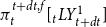
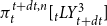








By combining (E1)–(E3) and stretching $dt$
towards
$dt$
towards $0$
, we derive the following
$0$
, we derive the following
 \begin{align*} lm^{(1)}+ \alpha _{t} \times lm^{(2)}=0, \end{align*}
where
 \begin{equation} lm^{(1)}=\lim \limits _{dt \rightarrow 0}\frac {\mathbb{E }_{\mathcal{F}_{t}}^{\mathbb{Z}_{\theta }^{a}\times \mathbb{Q}^{\,f}}\left[e^{-\int _{t}^{t+dt}r_s\textrm { d}s}\frac {N_{t+dt}}{N_t}\times \tilde {\pi }_{t+dt}\right] -\tilde {\pi }_{t}}{dt}, \end{equation}
and
 \begin{equation} lm^{(2)}=\lim \limits _{dt \rightarrow 0}P(t,t+dt) \times \sqrt {\frac {\mathbb{V }_{\mathcal{F}_{t}}\Big [\frac {N_{t+dt}}{N_t}\times \tilde {\pi }_{t+ dt}-\mathbb{E}_{\mathcal{F}_{t}\lor \mathfrak{S}_{t+dt} \lor \mathcal{F}_{t+dt}^f}\Big [\frac {N_{t+dt}}{N_t}\times \tilde {\pi }_{t+ dt}\Big ]\Big ]}{dt}}. \end{equation}
To resolve the limit $lm^{(1)}$
, we apply Itô’s lemma to
$lm^{(1)}$
, we apply Itô’s lemma to $\tilde {\pi }_{t+\mathrm{d}t}$
under the probability measure
$\tilde {\pi }_{t+\mathrm{d}t}$
under the probability measure $\mathbb{Z}_{\theta }^{a}\times \mathbb{Q}^{\,f}$
, where the dynamics of the stochastic mortality rates under
$\mathbb{Z}_{\theta }^{a}\times \mathbb{Q}^{\,f}$
, where the dynamics of the stochastic mortality rates under $\mathbb{Z}_{\theta }^{a}$
are obtained from the density equation (15) and are therefore given by
$\mathbb{Z}_{\theta }^{a}$
are obtained from the density equation (15) and are therefore given by
 \begin{align*} d\lambda _t=\left(\overline {\theta _{t,T}^{(1)}}+\mu _m\lambda _t\right) dt+\sigma _m dW_{m}^{*}(t), \end{align*}
with $\overline {\theta _{t,T}^{(1)}}=\theta _{0,T}^{(1)}\sigma _{m}^{2}\times \frac {e^{\mu _{m}(T-t)}-1}{\mu _m},$
and
$\overline {\theta _{t,T}^{(1)}}=\theta _{0,T}^{(1)}\sigma _{m}^{2}\times \frac {e^{\mu _{m}(T-t)}-1}{\mu _m},$
and $dW_{m}^{*}(t)=dW_{m}(t)- \theta _{0,T}^{(1)} \sigma _m \frac {e^{\mu _m(T-t)}-1}{\mu _m} \ \textrm {d}t.$
Let us denote $dW^{\rho }(s)=\rho dW_r(t)+\sqrt {1-\rho ^2}dW_S(t),$
then by employing Ito’s lemma with jump process under
$dW^{\rho }(s)=\rho dW_r(t)+\sqrt {1-\rho ^2}dW_S(t),$
then by employing Ito’s lemma with jump process under $\mathbb{Z}_{\theta }^{a}\times \mathbb{Q}^{f},$
we obtain
$\mathbb{Z}_{\theta }^{a}\times \mathbb{Q}^{f},$
we obtain
 \begin{align*} \tilde {\pi }_{t+dt} &=\tilde {\pi }_{t}+\int _{t}^{t+dt}\partial _{t} \tilde {\pi }_{s}ds+\int _{t}^{t+dt}\partial _{S} \tilde {\pi }_{s} r_{s}S_{s}ds+\sigma _{S}\int _{t}^{t+dt}\partial _{S}\tilde {\pi }_{s}S_{s}dW^{\rho }(s)\\&\quad +\int _{t}^{t+dt} (\theta -ar_{s})\partial _{r}\tilde {\pi }_{s}ds+ \sigma _{r}\int _{t}^{t+dt}\partial _{r}\tilde {\pi }_{s}dW_{r}(s)+\int _{t}^{t+dt} \left(\overline {\theta _{s,T}^{(1)}}+\mu _m\lambda _s\right)\partial _{\lambda }\tilde {\pi }_{s}ds\\&\quad +\sigma _{m}\int _{t}^{t+dt}\partial _{\lambda }\tilde {\pi }_{s}dW_{m}^{*}(s)+\frac {1}{2}\sigma _{S}^{2}\int _{t}^{t+dt}\partial _{S}^{2}\tilde {\pi }_{s}S_{s}^{2}ds+\frac {1}{2}\sigma _{m}^{2}\int _{t}^{t+dt}\partial _{\lambda }^{2}\tilde {\pi }_{s}ds\\&\quad +\frac {1}{2}\sigma _{r}^{2}\int _{t}^{t+dt}\partial _{r}^{2}\tilde {\pi }_{s}ds+\rho \sigma _{r} \sigma _{S}\int _{t}^{t+dt}\partial _{rS}^{2}\tilde {\pi }_{s}S_{s}ds+\int _{t}^{t+dt}(\tilde {\pi }^{*}_{s}-\tilde {\pi }_{s})dN_{s}, \end{align*}
where $\tilde {\pi }^{*}_{s}$
denotes the time-consistent value just before the jump in the number of survivors, i.e.
$\tilde {\pi }^{*}_{s}$
denotes the time-consistent value just before the jump in the number of survivors, i.e. $\tilde {\pi }^{*}_{s}[.]=\tilde {\pi }_{s}[.|N_{s}-1].$
By applying the discount factor multiplication
$\tilde {\pi }^{*}_{s}[.]=\tilde {\pi }_{s}[.|N_{s}-1].$
By applying the discount factor multiplication $e^{-\int _{t^{t+dt}}r_s\textrm {d}s}$
, we subsequently engage in the calculation of the mathematical expectation to reach
$e^{-\int _{t^{t+dt}}r_s\textrm {d}s}$
, we subsequently engage in the calculation of the mathematical expectation to reach
 \begin{align*} lm^{(1)} &=\tilde {\pi }_{t}\lim \limits _{dt \rightarrow 0}\frac {\mathbb{E }_{\mathcal{F}_{t}}^{\mathbb{Z}_{\theta }^{a} \times \mathbb{Q}^{\,f}}\!\left[\frac {N_{t+dt}}{N_t}\times e^{-\int _{t}^{t+dt}r_s\textrm {d}s} \right]{-}1}{dt}+\lim \limits _{dt \rightarrow 0}\frac {\int _{t}^{t+dt}\mathbb{E }_{\mathcal{F}_{t}}^{\mathbb{Z}_{\theta }^{a} \times \mathbb{Q}^{\,f}}\!\left[\frac {N_{t+dt}}{N_t}\times e^{-\int _{t}^{t+dt}r_s\textrm {d}s} \partial _{t} \tilde {\pi }_{s}\right]ds}{dt}\\&\quad +\lim \limits _{dt \rightarrow 0}\frac {\int _{t}^{t+dt}\mathbb{E }_{\mathcal{F}_{t}}^{\mathbb{Z}_{\theta }^{a} \times \mathbb{Q}^{\,f}}\left[\frac {N_{t+dt}}{N_t}e^{-\int _{t}^{t+dt}r_s\textrm {d}s}\partial _{S} \tilde {\pi }_{s}r_{s}S_{s}\right]ds}{dt}\\&\quad + \sigma _{S}\lim \limits _{dt \rightarrow 0}\frac {\int _{t}^{t+dt}\mathbb{E }_{\mathcal{F}_{t}}^{\mathbb{Z}_{\theta }^{a} \times \mathbb{Q}^{\,f}}\left[\frac {N_{t+dt}}{N_t}e^{-\int _{t}^{t+dt}r_s\textrm {d}s} \partial _{S} \tilde {\pi }_{s}S_{s}dW^{\rho }(s)\right]}{dt}\\&\quad +\lim \limits _{dt \rightarrow 0}\frac {\int _{t}^{t+dt}\mathbb{E }_{\mathcal{F}_{t}}^{ \mathbb{Z}_{\theta }^{a}\times \mathbb{Q}^{\,f}}\left[\frac {N_{t+dt}}{N_t}e^{-\int _{t}^{t+dt}r_s\textrm {d}s} \partial _{r} \tilde {\pi }_{s}(\theta -ar_{s})\right]ds}{dt}\\&\quad +\sigma _{r}\lim \limits _{dt \rightarrow 0}\frac {\int _{t}^{t+dt}\mathbb{E }_{\mathcal{F}_{t}}^{ \mathbb{Z}_{\theta }^{a}\times \mathbb{Q}^{\,f}}\left[\frac {N_{t+dt}}{N_t} e^{-\int _{t}^{t+dt}r_s\textrm {d}s}\partial _{r} \tilde {\pi }_{s}dW_{r}(s)\right]}{dt}\\&\quad + \lim \limits _{dt \rightarrow 0}\frac {\int _{t}^{t+dt}\mathbb{E }_{\mathcal{F}_{t}}^{\mathbb{Z}_{\theta }^{a} \times \mathbb{Q}^{\,f}}\left[\frac {N_{t+dt}}{N_t}\times e^{-\int _{t}^{t+dt}r_s\textrm {d}s}\left(\overline {\theta _{s,T}^{(1)}}+\mu _m\lambda _s\right)\partial _{\lambda } \tilde {\pi }_{s}\right]ds}{dt} \\&\quad +\frac {\sigma _{S}^2}{2}\lim \limits _{dt \rightarrow 0}\frac {\int _{t}^{t+dt}\mathbb{E }_{\mathcal{F}_{t}}^{ \mathbb{Z}_{\theta }^{a}\times \mathbb{Q}^{\,f}}\left[\frac {N_{t+dt}}{N_t} e^{-\int _{t}^{t+dt}r_s\textrm {d}s}\partial _{S}^{2} \tilde {\pi }_{s}S_{s}^{2}\right]ds}{dt}\\&\quad + \frac {\sigma _{m}^2}{2}\lim \limits _{dt \rightarrow 0}\frac {\int _{t}^{t+dt}\mathbb{E }_{\mathcal{F}_{t}}^{\mathbb{Z}_{\theta }^{a} \times \mathbb{Q}^{\,f}}\left[e^{-\int _{t}^{t+dt}r_s\textrm {d}s} \frac {N_{t+dt}}{N_t}\partial _{\lambda }^{2} \tilde {\pi }_{s}\right]ds}{dt}\\&\quad + \frac {\sigma _{r}^2}{2}\lim \limits _{dt \rightarrow 0}\frac {\int _{t}^{t+dt}\mathbb{E }_{\mathcal{F}_{t}}^{\mathbb{Z}_{\theta }^{a} \times \mathbb{Q}^{\,f}}\left[\frac {N_{t+dt}}{N_t} e^{-\int _{t}^{t+dt}r_s\textrm {d}s}\partial _{r}^{2} \tilde {\pi }_{s}\right]ds}{dt}\\&\quad + \rho \sigma _{S} \sigma _{r}\lim \limits _{dt \rightarrow 0}\frac {\int _{t}^{t+dt}\mathbb{E }_{\mathcal{F}_{t}}^{ \mathbb{Z}_{\theta }^{a}\times \mathbb{Q}^{\,f}}\left[\frac {N_{t+dt}}{N_t} e^{-\int _{t}^{t+dt}r_s\textrm {d}s}\partial _{Sr}^{2} \tilde {\pi }_{s}S_{s}\right]ds}{dt}\\&\quad +\lim \limits _{dt \rightarrow 0} \frac {\int _{t}^{t+dt} \mathbb{E }_{\mathcal{F}_{t}}^{ \mathbb{Z}_{\theta }^{a}\times \mathbb{Q}^{\,f}}\left[\frac {N_{t+dt}}{N_t} e^{-\int _{t}^{t+dt}r_s\textrm {d}s}(\tilde {\pi }^{*}_{s}-\tilde {\pi }_{s})dN_{s}\right]}{dt}\\&\quad + \sigma _{m}\lim \limits _{dt \rightarrow 0}\frac {\int _{t}^{t+dt}\mathbb{E }_{\mathcal{F}_{t}}^{\mathbb{Z}_{\theta }^{a} \times \mathbb{Q}^{\,f}}\left[\frac {N_{t+dt}}{N_t} e^{-\int _{t}^{t+dt}r_s\textrm {d}s}\partial _{\lambda } \tilde {\pi }_{s} dW_{m}^{*}(s)\right]ds}{dt}.\\ &=-r_{t}\tilde {\pi }_{t}+\partial _{t} \tilde {\pi }_{t}+r_{t}S_{t}\partial _{S} \tilde {\pi }_{t}+(\theta -ar_{t})\partial _{r} \tilde {\pi }_{t}+\big(\overline {\theta _{t,T}^{(1)}}+\mu _m \lambda _t\big)\partial _{\lambda } \tilde {\pi }_{t}+\frac {1}{2}\sigma _{S}^{2}S_{t}^{2}\partial _{S}^{2}\tilde {\pi }_{t}\\ &\quad +\frac {1}{2}\sigma _{m}^{2}\partial _{\lambda }^{2}\tilde {\pi }_{t} +\frac {1}{2}\sigma _{r}^{2}\partial _{r}^{2}\tilde {\pi }_{t} + \rho \sigma _{r}\sigma _{S}S_{t}\partial _{rS}^{2}\tilde {\pi }_{t}+(\tilde {\pi }^{*}_{t}-\tilde {\pi }_{t})\lambda _{t}. \end{align*}
Regarding the second limit $lm^{(2)}$
, to resolve it, we use the fact that
$lm^{(2)}$
, to resolve it, we use the fact that $\mathbb{V}_{\mathcal{F}_{t}}\Big [\frac {N_{t+dt}}{N_t}\times \tilde {\pi }_{t+ dt}-\mathbb{E}_{\mathcal{F}_{t}\lor \mathfrak{S}_{t+dt} \lor \mathcal{F}_{t+dt}^f}\Big [\frac {N_{t+dt}}{N_t}\times \tilde {\pi }_{t+ dt}\Big ]\Big ] = \mathbb{E}_{\mathcal{F}_{t}}\Big [\mathbb{V}_{\mathcal{F}_{t}\lor \mathfrak{S}_{t+dt} \lor \mathcal{F}_{t+dt}^f}\Big [\frac {N_{t+dt}}{N_t}\times \tilde {\pi }_{t+ dt}\Big ]\Big ]$
and apply Itô’s lemma to
$\mathbb{V}_{\mathcal{F}_{t}}\Big [\frac {N_{t+dt}}{N_t}\times \tilde {\pi }_{t+ dt}-\mathbb{E}_{\mathcal{F}_{t}\lor \mathfrak{S}_{t+dt} \lor \mathcal{F}_{t+dt}^f}\Big [\frac {N_{t+dt}}{N_t}\times \tilde {\pi }_{t+ dt}\Big ]\Big ] = \mathbb{E}_{\mathcal{F}_{t}}\Big [\mathbb{V}_{\mathcal{F}_{t}\lor \mathfrak{S}_{t+dt} \lor \mathcal{F}_{t+dt}^f}\Big [\frac {N_{t+dt}}{N_t}\times \tilde {\pi }_{t+ dt}\Big ]\Big ]$
and apply Itô’s lemma to $\tilde {\pi }_{t+ dt}$
and
$\tilde {\pi }_{t+ dt}$
and $\tilde {\pi }_{t+ dt}^{2}$
under
$\tilde {\pi }_{t+ dt}^{2}$
under $\mathbb{P}=\mathbb{P}^{a}\times \mathbb{P}^{f}$
. Following a similar calculation and algebraic simplification as before to compute
$\mathbb{P}=\mathbb{P}^{a}\times \mathbb{P}^{f}$
. Following a similar calculation and algebraic simplification as before to compute $lm^{(1)}$
, and considering the continuity property of the root function, and applying the rule that the product of two existing finite limits equals the limit of the product, we then obtain
$lm^{(1)}$
, and considering the continuity property of the root function, and applying the rule that the product of two existing finite limits equals the limit of the product, we then obtain
 \begin{align*} lm^{(2)} &=\sqrt { \sigma _{S}^{2}S_{t}^{2}(\partial _{S}\tilde {\pi }_{t})^{2}+\sigma _{m}^{2}(\partial _{\lambda }\tilde {\pi }_{t})^{2}+\sigma _{r}^{2}(\partial _{r}\tilde {\pi }_{t})^{2}+2\rho \sigma _{S}\sigma _{r}S_{t}\times \partial _{S}\tilde {\pi }_{t}\partial _{r}\tilde {\pi }_{t}+(\tilde {\pi }_{t}-\tilde {\pi }_{t}^{*})^{2}\lambda _{t} }\\ &\quad \times \lim \limits _{dt \rightarrow 0} P(t,t+dt)\\ &=\sqrt { \sigma _{S}^{2}S_{t}^{2}(\partial _{S}\tilde {\pi }_{t})^{2}+\sigma _{m}^{2}(\partial _{\lambda }\tilde {\pi }_{t})^{2}+\sigma _{r}^{2}(\partial _{r}\tilde {\pi }_{t})^{2}+2\rho \sigma _{S}\sigma _{r}S_{t}\times \partial _{S}\tilde {\pi }_{t}\partial _{r}\tilde {\pi }_{t}+(\tilde {\pi }_{t}-\tilde {\pi }_{t}^{*})^{2}\lambda _{t} }. \end{align*}











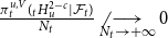









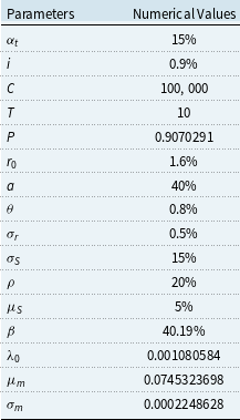
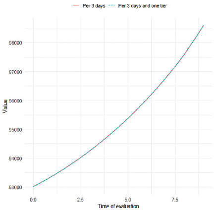


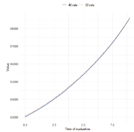


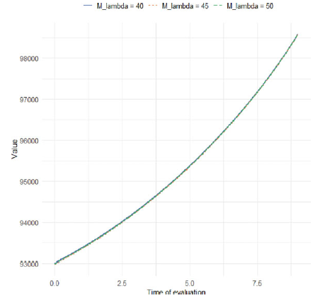


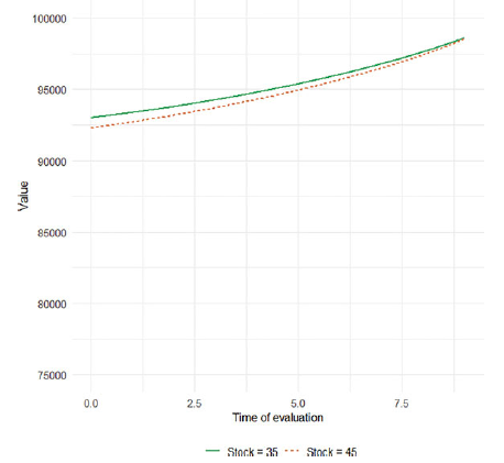


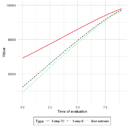


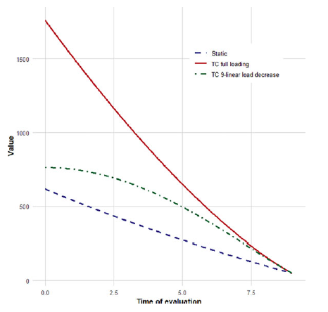


 Open access

