
In the United States, children from a low-income family are less likely to consume the daily recommended amount of fruits and vegetables than are children from a high-income family (Rasmussen et al. Reference Rasmussen, Krølner, Klepp, Lytle, Brug, Bere and Due2006). Some of these differences may stem from access (Larson, Story, and Nelson Reference Larson, Story and Nelson2009) or the fact that fruits and vegetables are perceived as more expensive (Cassady, Jetter, and Culp Reference Cassady, Jetter and Culp2007). However, schools provide a unique opportunity to provide children with free and easy access to fruits and vegetables, and there has been considerable effort to include more fruits and vegetables in the breakfast and lunch offerings and in snack programs supported by USDA. In fact, most children in the United States do not meet dietary recommendations and would benefit from an improved diet, including high-income children (Story Reference Story2009).
Over 70% of children eat school lunch three or more times per week (Wansink et al. Reference Wansink, Just, Patterson and Smith2013), and recent estimates indicate that about 77% of children eat school lunch three or more times per week (CDC and NCHS 2018). Many children also eat breakfast at school, receive meals during the summer, are given food to take home over the weekend, and are sometimes even offered dinner when they stay for after-school programs. The combination of these programs means that some kids have the potential to eat more of their meals at school than at home. This provides a unique opportunity for schools to influence the amount of fruits and vegetables that children eat. However, the habits that children form at home may affect their willingness to consume fruits and vegetables even when they are offered for free at school. Thus, additional approaches are required to help children tap into the access they have to fruits and vegetables at school.
Behavioral economics provides a number of tools that can be used to encourage children to consume more fruits and vegetables at school. Many of these tools fall under the category of nudges, as described by Thaler and Sunstein (Reference Thaler and Sunstein2008), and the Healthy Lunchroom Initiative provides an even more expanded list of these approaches (Just and Wansink Reference Just and Wansink2009). Possible interventions can be based on incentives, default options, choice architecture, competition, messaging, and pre-commitment. Interventions can also include removing competing foods (like snacks that can be purchased individually), increasing the variety of fruit and vegetable options, and embedding fruits and vegetables as an integral part of other items (like smoothies), associating fruits and vegetables with something cool (like the Food Dudes program [Wengreen et al. Reference Wengreen, Madden, Aguilar, Smits and Jones2013]), and moving recess to before lunch. There is a growing amount of research that documents the efficacy of many of these interventions. The focus of this article is on providing some practical advice about how to conduct a research study in schools to evaluate the impact of a particular intervention.
I start with an intervention that has not been rigorously evaluated by academic researchers but was piloted by a school nutrition company called Nutrislice (www.nutrislice.com). It is an interesting intervention that helps frame the issues related to evaluating the impact of a specific intervention. Nutrislice ran a competition during lunch between adjacent grades in which it recorded and reported in real time the number of servings of broccoli that had been consumed. The grade that won the competition would have each student be given a small smoothie. Figure 1 shows the setup of the intervention. The two grades were closely matched during the competition, and the figure provides a picture of the kids as they began to chant “Eat your broccoli!” while watching updates in the numbers on a large screen that had been set up. In the end, the children at that school consumed several times more broccoli that day than had been observed on any other previous days.
Nutrislice Broccoli Competition

This was a one-time pilot study that had a huge effect on the amount of broccoli that children ate. The question is what to do with this information. Should every school have a broccoli competition? How often should the school do it? Would we want to do it every day? The ability to answer these questions relies on the degree to which a particular intervention will have a sustained effect over time, the cost of implementing the intervention, and whether a one-day intervention will have positive or negative effects in the long run when the intervention is concluded. Additionally, the answers to these questions depend on the external validity of the experiment and whether or not the results are generalizable to a broader population. Whether or not a specific intervention should be implemented in a large number of schools depends on if the intervention will have a similar effect in most schools where it is implemented. This particular intervention includes some interesting elements of competition, real-time feedback, peer pressure, and incentives.
It would be helpful to design variants of the experience that remove different aspects of the intervention to see which underlying behavioral motivations seem to be the most important. For example, it would be interesting to see if the same approach would work even if there hadn't been any smoothies offered to the winners. This would certainly improve the cost-effectiveness of the program. Providing real-time feedback is a logistical challenge and requires some technology to be in place. It would be helpful to test how much the impact of the intervention drops without that component. Finally, it would be important to see what happens in the school the next time broccoli is served so that we can see what the long-run effects of the intervention are.
The exciting thing is that schools will find creative ways to encourage children to eat in a more healthy way. Because of this, it is important to have a rigorous way to evaluate the impact of the intervention and to be able to frame the degree to which the intervention affects student behavior both during the intervention and after it is removed. This provides a unique opportunity for academics who develop tools and empirical strategies that allow them to collaborate with schools to evaluate school-based interventions. There might even be ways that students themselves could be equipped with the tools to carry out a well-designed experiment as part of a science fair project and collect data in ways in which they can be aggregated and evaluated by researchers.
The sections that follow describe several issues that are important to consider when conducting a field experiment in a school. Each of these issues arose in the course of my own field experiments in schools, and the hope is that the lessons we learned will be helpful to scholars considering doing research in schools. The focus of my experiments has been on encouraging children to eat more fruits and vegetables, but the issues addressed are relevant to interventions that influence other behaviors or decisions that children make at school.
Data Collection
All empirical studies will require some form of data collection. When I first started working in this area, I met with the nutrition directors of different school districts to better understand the type of data that they were gathering. Nearly all schools collect production records on the number of items that were served during each lunch. This is usually based on calculating the amount of each item that was used in preparing the meals for that meal and then subtracting out the amount of each item that is left over. This will provide a good aggregate measure of what is served but does not account for any waste that occurs when children discard their trays. In addition, it doesn't provide information at the individual level, which can be important if we want to see how the effect of an intervention differs by grade or gender.
Many schools also have data from a point-of-sale (POS) system. The advantages of this data are that they will provide information on the item-level choices that children make. For example, many POS systems will record the exact fruit and vegetable items that children take, which entrée they choose, and whether they take white or chocolate milk. Since these data are already collected by the school, if researchers can access these data, then they can get a very long-run look at the behavior before, during, and after the intervention, which is a huge advantage. The main disadvantage is that the data don't provide any information about whether the child actually ate the items.
In addition to the POS and aggregate data, school administrative data that contain information about the characteristics of the schools involved in your experiment can be useful. The Common Core of Data (CCD) provided by the National Center for Education Statistics (NCES) contains useful demographic data such as gender, ethnicity, and grade level distribution. This data source also contains information relevant to school lunch participation, such as the fraction of students who are eligible to receive a free or reduced-price lunch (FRPL). The Food Research and Action Center (FRAC) provides statistics on the Identified Student Population (ISP), which is the percentage of students in a school that come from households receiving government welfare assistance. These administrative data can be used to compare characteristics between treatment and control schools.
In order to collect consumption data, you need to have some way of observing the child's tray at the end of lunch so you can see which items were not consumed. There have been several methods developed to provide an accurate measure of the amount of each item that the child consumed. Some of these involve weighing items from the tray at the start and end of lunch (Getlinger et al. Reference Getlinger, Laughlin, Bell, Akre and Arjmandi1996). Others involve taking a picture of the tray at the start and end of lunch and then using researchers to evaluate the amount consumed based on the pictures (Swanson Reference Swanson2008). All of these methods involve collecting data at the start and end of lunch and generally require that you take a random sample of students to follow, because these methods can be very time-intensive. In addition, since you are gathering data on specific students, this approach generally requires active parental consent for the child to participate.
Based on some pilots we did, we ultimately decided to take a different approach to gathering data that has some nice features that would allow the data to be easily used by other researchers. One of the advantages of measuring consumption of fruits and vegetables is that they come in pre-portioned amounts and leave behind a cup or peel that allows us to observe the numbers of items that were taken. This makes it possible to gather the data using only observations taken at the end of lunch. We would have our research assistants stand in the cafeteria near the place where students discard their trays and record information—the child's grade, age, entrée choice, and the number of servings of each fruit and vegetable that they took and consumed. While this approach worked for the schools in our experiment, it would likely need to be adjusted for different schools, such as schools with a salad bar where students can serve themselves.
Figure 2 is a picture of the iPhone app that we developed to gather data. In the particular case shown, the child had taken two servings of broccoli and one serving of green beans. They had consumed 1.5 servings of broccoli but none of the green beans. The disadvantage of this approach is that the data are gathered rather quickly, and the consumption amounts are less precisely measured than in other approaches. The key advantage is that our method requires about 40 hours of research assistant time to collect 10 days of data at one school. Thus, for a cost of about $340 in research assistant wages, you can gather 3,000 student-day observations. We were even able to find ways to hire parents from the school to gather data for us, which reduced the travel costs of collecting data and allowed us to expand the geographic scope of the schools we work with.
VProject iPhone App for Data Collection

In addition to collecting data on what is served, it is also helpful to take pictures each day of the setup of the cafeteria, the layout of the way food is served, and the specific items that are served that day. These pictures allow future researchers to create measures from your experiment that expand the use of the data you collect to answer other questions. It is also helpful in framing the issue to public audiences, because they often have a misperception about the quality of fruits and vegetables being served in schools. Figure 3 provides some examples of photos that we took in the schools that we were working with. Most of the parents that we've shared these photos with have been surprised by the quality and attractiveness of the items being served in schools. With advances in machine learning, there might even be innovative ways these pictures could be used in future research to provide quantitative measures of the items being served each day.
Example Pictures of Fruit and Vegetable Items Served in Our Sample

Baseline Data
A key component of your study will be to establish what the baseline pattern of consumption is at the school. For our experiments, we have tried to collect at least 5–10 days of baseline data at each school. The larger baseline period will be important in terms of statistical power, since the intervention effect will be evaluated relative to this baseline measure. For our original experiment on incentives (Just and Price Reference Just and Price2013), we collected five days of baseline data at each of the 15 schools. This provided 30,550 child-day observations and made it possible to establish a reasonable baseline at each school. From this baseline data, we learned that 33.5% of children ate at least one serving of fruits and vegetables each day, and this rate was higher for girls and older children. We also learned that 42.7% of the fruits and vegetables being served were ending up in the trash; this was a surprise to the nutrition directors we were working with, as all of their previous estimates of consumption and waste had been based on production records.
The baseline data also provide an important role in mitigating concerns about a Hawthorne effect. It is true that every intervention we evaluate has the possibility that having people in the cafeteria gathering data will influence children's behavior. One way to reduce this concern is to have researchers located in as inconspicuous a place as possible and to have them answer questions about what they are doing in non-specific ways that don't reflect the fact that they are gathering data on fruits and vegetables. In one of our experiments (O'Bryan, Price, and Riis Reference O'Bryan, Price and Riis2017), the students place their trays on a conveyor belt, and so we were able to gather the data on the other side of the wall, out of sight. Having a longer baseline data collection period helps to reduce the novelty effect you might pick up the first day data collectors are present. You can also test to see if there is a trend during the baseline period, and we find that there is a slight negative trend. This means that your baseline data are likely to reflect the true behavior once you have been collecting data for enough days.
Control Schools
Another related issue is the use of control schools. The difference-in-difference model is a commonly used empirical strategy in policy evaluation. This involves having pre-intervention and post-intervention data for a treatment and a control group. The control group serves two important functions in this approach. First, it accounts for any other changes that might have occurred at the same time the treatment started. Second, it helps account for any Hawthorne Effect of being in the treatment group. The disadvantages of including a control group is that it adds to the cost of running the experiment. It can also make it hard to recruit schools to participate in the study. It can often be difficult to recruit schools, especially when they are told there is a chance they will participate without any possible benefits for their students.
One approach we used in a large field experiment with 40 schools (Loewenstein, Price, and Volpp Reference Loewenstein, Price and Volpp2016) was randomizing the timing of when the treatment began. As a result, some schools started in October, others in November, and so on through the school year. This allowed us to use the staggered baseline periods to capture any changes over time in other factors that might influence the outcome. To address the concern about the Hawthorne Effect, we used a 10-day baseline period so the students could fully adjust to having data collectors in the cafeteria before we started the treatment. Another benefit of the staggered approach is that it allowed us to work with 40 schools and not have to hire nearly as many research assistants as we would have needed if we had done all the schools at the same time. When research assistants completed their experiment at one school, they would move on to the next school, which allowed the inclusion of data from about four times as many schools with the same number of research assistants.
Level of Randomization
Another important decision is the level of randomization to use. The unit of observation that you use for your randomization will have a large effect on the statistical power you have for your experiment. If you can randomize at the individual level, then you could have over 500 randomization units in one school. In contrast, if you randomize at the classroom level, this could drop to 20, or at the grade level, it could drop to six. When you do inference, you will want to cluster your standard errors at the level of randomization that you used in your experiment. Thus you'll want to use the randomization unit that is the most reasonable for your experiment. When choosing between options with similar benefits, opt for the approach that will give you the most randomization units.
All of the experiments that I have done have involved school-level randomization. There were four reasons we chose to use school-level randomization instead of student-level randomization. First, in many cases, we wanted to be able to get maximum advertising for the intervention once it started. For an incentive experiment, we wanted to be able to include a morning announcement for the whole school about the new program. Second, we wanted to avoid any contamination effects. This could occur if children learned of others getting a reward for eating a serving of fruits and vegetables and then changed their behavior because they thought the same would be true for themselves. Third, we wanted to avoid any reactance effects that might occur if members of the control group felt it was unfair that they were being treated differently. Fourth, we wanted to be able to use an opt-out consent form for participation in our experiment, which was only justified on the basis that the entire school was getting the same treatment.
A modified approach would cost much less to implement and would preserve many of the nice features of school-level randomization. When the randomization unit is the school, then you don't get a lot of extra statistical power from having more student observations within the school. Having more students does improve the precision of your estimates a bit, but not nearly as much as having additional schools. Thus, with a fixed budget it might make sense to consider only included students from a specific grade or lunch period in the experiment. It might also make sense to focus on schools that have a smaller student body. Both of these decisions will mean you will have a smaller subject pool within each school, which will make it less costly to implement some experiments (like those that involve incentives) or to collect the data (since at big schools, we often needed to send two to three research assistants to collect the data). School size is an important factor to consider, because it is possible that focusing on smaller schools potentially excludes urban schools or secondary schools. In our experiments, we focus on fruit and vegetable consumption in elementary schools rather than secondary schools, so our results are more generalizable to the elementary school population. Whether experiment results are generalizable to urban schools depends on whether or not the key difference between urban and non-urban schools is school size. The key concern with these approaches depends on whether you think the effect of the treatment differs by grade or school size. In the work we've done, we find that baseline levels of fruit and vegetable consumption differ by grade but that the treatment effect does not differ by grade or school size. Thus, if the key difference between urban and non-urban schools is size, it appears that our experiment results are generalizable to urban schools.
Heterogeneous Treatment Effects
There will be some experiments, however, where you will want to know how the treatment effect differs based on student or school characteristics. These heterogeneous treatment effects can help in understanding which groups to target different interventions toward and can provide insight into how an intervention might create differences in outcomes between groups. In our experiments about the effect of incentives, we did not find any differences in the effect of incentives based on gender or grade. However, we did find very large differences based on income level.
We had originally explored some ways to identify the free or reduced-price lunch (FRPL) status of individual students, but it just never worked very well, given the way we were collecting our data. As a result, instead of using individual-level data on FRPL status, we used measures we had about the fraction of students at the school that received a FRPL as a proxy for the income level of the school. In our estimation models, we then included an interaction between treatment and the FRPL rate for the school.
This turned out to be a very informative interaction term that indicated that the effect of the incentives at the poorest schools in our sample (FRPL = 77%) was over twice as large as at the richest schools in our sample (FRPL = 17%). This suggests that incentives do a very good job of specifically targeting the students who are most likely to benefit from the intervention, since they are the ones least likely to be consuming fruits and vegetables at home.
Standard Errors
In a previous section, I mentioned the importance of clustering your standard errors at the level of randomization (student, class, grade, school, etc.). There is a real challenge with having too few randomization units, because the ability to cluster the standard errors can become problematic. The experiment in Just and Price (Reference Just and Price2013) had only 15 schools. The editor of the first journal we submitted our article to commented that it just didn't seem possible to do inference with only 15 clusters. There are other approaches to doing inference when you have a small number of clusters. One option is to collapse your data down to the level of variation.
Thus, instead of doing your inference on student-level data about what they consumed, you can get an observation for each school from its pre period and one from its post period. This approach would not require you to cluster your standard but would leave you with a much smaller sample than you originally thought. This has the benefit of not letting a large sample size give the illusion that you have a lot of insightful variation in your data. With your collapsed data you can even do a Fisher's exact test, where you take each of your schools and label them as treatment or control, based on their status. You then give schools individually an indicator based on whether they had an increase in behavior above some threshold. Then you use the Fisher's exact test to determine the probability of observing by chance the pattern that you see in your data. In Just and Price (Reference Just and Price2013), we found that all 13 treatment schools had a positive increase, while the two control schools did not. The probability of observing this pattern by chance is 0.0095, which provides insight about inference similar to a p-value.
Another approach in these settings is to use permutation inference. In Loewenstein, Price, and Volpp (Reference Loewenstein, Price and Volpp2016), we had 40 schools in our sample; 19 were given incentives for five weeks, and 21 were given incentives for three weeks. We wanted to test if the long-run effects of incentives were larger when the incentives were in place for a longer period of time. We had used several methods for calculating the standard errors of one of our key estimates, including generalized estimating equations, wild bootstrap, and paired bootstrap. All of these provided a p-value of our parameter of interest right near 0.05, but some were above that threshold and some were below.
We decided to use permutation inference because it has a few features that provided a more transparent way of testing the likelihood that there was a real difference in outcomes between the two treatment groups. First, we randomly generated permutations of each of the possible labels for each school and then reestimated our model under 10,000 of these permutations. This means that whether a school was labeled as in the five-week treatment group or three-week treatment group was randomly assigned and then the model was estimated as though that had been the correct assignment. This provided a distribution of coefficients from our model under all of the permutations. We then compared this distribution to the coefficient that we obtained with the correctly labeled schools. Of the 10,000 permutations, there were 246 that had a coefficient higher than what we found, providing a p-value of 0.049 (see Figure 4).
Graphs Based on Permutation Inference
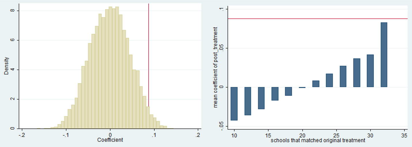
In addition, when we put the coefficients into categories based on the number of schools that had been labeled correctly by accident during the random assignment, we found the largest coefficients for those permutations where the highest fraction of schools had been labeled correctly (see Figure 4). If there had been no true treatment effect, then we would expect the average coefficients to be similar across the different bins.
An approach similar to permutation inference can play a particularly important role in experiments where there is a very low cost of collecting baseline or control data but a very high cost of collecting treatment data. For example, if the outcome you are interested in could be collected using data from a POS system, then it might be possible to obtain tens of thousands of observations for nearly free. You can use these data to establish a well-defined distribution for what you would expect the outcomes to be on typical data. Then, if you implement your treatment for even one day, you can compare that observation to this well-defined distribution to obtain the probability of observing that outcome by chance. While most would not want to recognize a result based on one treatment observation, the principle is that permutation inference can provide a relatively transparent way to observe the likelihood of observing a particular outcome by chance, and this insight can be pretty clear even with only a few treatment observations.
Aggregation of Marginal Effects
Some of the interventions that we will use might provide only a small nudge. It is important to look for ways to aggregate these marginal effects in a way to amplify the final impact. One example of this is the type of incentive that we used in the habit formation experiment with 40 schools. In my earlier experiment with David Just, we had used cash prizes. Cash prizes turned out to be the most effective incentive to use in our setting but did have the downsides of the kids using the money mostly to buy candy and of an uptick in bullying in the school. As a result, for our larger experiment, we decided to use a veggie coin instead of cash. The veggie coin was worth a quarter but could only be used at the school store (which was not allowed to sell candy).
Figure 5 shows the image that was on the coin. It turns out that the use of the veggie coin had three important benefits over cash. First, the image on the coin provided a tangible reminder of the action the children had taken to receive the reward. Second, since all of the veggie coins were redeemed at the school store, it made it easier logistically to make the cash disbursements. We would simply write the PTA a check at the end of the experiment based on the number of veggie coins that were redeemed, which we could also check against the data collection on the number of kids who received a coin. Third, many schools only had the school store open once a week or at the end of the incentive period. The kids would then accumulate their coins over time, which would make the perceived marginal benefit of consuming a serving of fruits and vegetables each day seem larger as well. This technique is often used by financial planners who emphasize that small changes in spending each day can aggregate into very large changes in spending over time.
Veggie Coin Used in Habit Formation Experiment

Conclusion
The goal of this article was to point out some issues that are helpful to consider when designing a field experiment to encourage healthy eating in schools. These experiments have the added benefit of providing general behavioral insights about interventions that might work for behaviors outside the specific focus of healthy eating, such as academic performance or exercise. My hope is that more researchers will consider collaborating with schools to test the effect of different interventions that can influence positive behaviors in children. This research can be very personally rewarding and have an impact on schools. The study I did with David Just about the impact of moving recess before lunch was picked up by the media and has led lots of schools and districts to adopt this simple change. In addition, many of the interventions you identify that work in schools might have applications in your own home or in your own daily choices.
Another important aspect to consider when examining the efficacy of interventions in schools is external validity, how well results generalize to a broader population. Schools serve students who range widely in age, from 6 to 18, and schools are often very different along socioeconomic and demographic characteristics. This should be considered when examining how well an intervention may work when implemented on a broader scale. In particular, one must consider how representative of the general school population the schools involved in an experiment are. Interventions should only be implemented on a broad scale if the experimental units are representative of the general population and as long as the intervention has been implemented multiple times with similar results. Ultimately, the most effective interventions that influence children to eat fruits and vegetables in school are those that are tested in internally valid experiments with a sample from which externally valid conclusions can be drawn.


 Open access