


1. Introduction
It is becoming more common for Bayesian techniques to be used to analyze data from economic experiments.Footnote 2 While their applications often aim to estimate similar parameters to their maximum-likelihood counterparts, such as parameters in utility functions, to estimate a Bayesian model the practitioner has one additional modeling choice: the prior. Here, we express our beliefs about the values of our model’s parameters before we observe any data. For Bayesian models, the prior is as much a part of the model as the likelihood: the likelihood is our formal statement of how our model’s parameters generate data conditional on parameter values, and the prior is our formal statement of our beliefs about the values of the model’s parameters before we observe new data.
Although we may have a good idea about what are likely and unlikely values for our model’s parameters, it is tempting to assign highly diffuse priors. If we want our estimates to be “driven mostly by our data”, and not be too influenced by our priors, then we may be tempted to choose priors that do not place too much mass on any small region of the parameter’s support. In the limit, this could be a uniform prior, but in practice this inclination typically manifests itself in the choice of an astronomically large prior variance. In addition to the obvious conflict between such diffuse priors and our domain expertise (e.g., our understanding of typical parameter values for our subject pool), these priors can also imply implausible distributions of economically meaningful quantities that we intend to calculate from our estimates.
In order to understand the implications of assigning highly diffuse priors, consider estimating a constant-only probit model:
 \begin{equation*}
\begin{array}{ll}
\text{likelihood:} & y\mid \theta \sim \mathrm{Bernoulli}\left(\Phi(\theta)\right)\\
\text{prior: }& \theta\sim N(m_\theta,s^2_\theta)
\end{array}
\end{equation*}
\begin{equation*}
\begin{array}{ll}
\text{likelihood:} & y\mid \theta \sim \mathrm{Bernoulli}\left(\Phi(\theta)\right)\\
\text{prior: }& \theta\sim N(m_\theta,s^2_\theta)
\end{array}
\end{equation*} where  $\Phi(\cdot)$ is the standard normal cumulative density function, and mθ and sθ are the prior mean and standard deviation of the model’s parameter θ, respectively. Since our data are binary, we might be interested in reporting the posterior distribution of
  $\Phi(\theta)$, which is the probability of success in the Bernoulli process. Suppose that we are happy setting
  $m_\theta=0$, which sets the median of
  $\Phi(\theta)$ to 0.5. However since we do not want our prior for θ to influence our estimates too much, we decide to set sθ to a large number. True, this will mean that the distribution of θ will be nicely spread out, but what does this say about
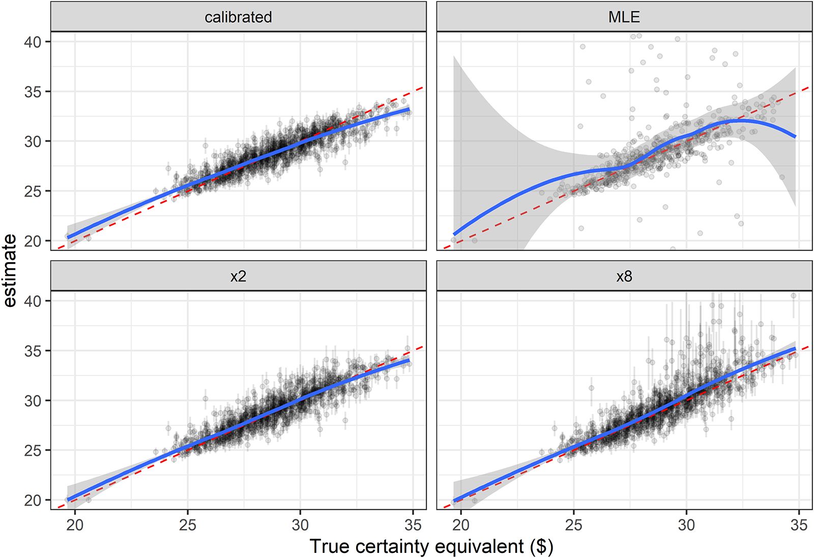
  $\Phi(\theta)$, which is the quantity we actually care about? Figure 1 shows 10,000 draws from this distribution, varying the prior standard deviation sθ. Note that even for modest choices of this variable, there are large accumulations of probability mass around 0 and 1. A highly diffuse prior for θ actually provides a lot of information about
  $\Phi(\theta)$: it is unlikely that the probability of success is anything other than 0 or 1. Put differently, if our data-generating process was a series of coin flips, our prior belief with
  $s_\theta=16$ means that we believe we are either flipping a coin with two heads, or a coin with two tails!Footnote 3
Draws from the prior distribution of  $\Phi(\theta)$, varying the standard deviation of θ

This may seem like a rather convoluted example, however note that many of the structural models we take to our data are also models of coin-flipping. Our “coin” is a participant’s choice between two options, and our model describes how this coin is weighted based on conditions of the experiment (e.g. two lotteries that a participant is choosing between) and parameters that we aim to estimate (e.g. a parameter in a utility function). These models often involve non-linear transformations of data and parameters in ways which, without careful consideration, can make predictions as implausible as the above example.
Even if we are comfortable with dissonance between our actual priors as experts in the field, and the priors we use in estimation, highly diffuse priors can greatly influence posterior estimates of economically meaningful quantities, such as welfare measures (e.g. Monroe, Reference Monroe, Harrison and Ross2023). These quantities are typically not fundamental parameters of our model, but can be easily computed once we have estimated a model’s parameters. As such, it is unlikely that any prior we choose will have negligible effect on our posterior estimates.
This calls for the use of the “Principled Bayesian Workflow”, as described by Betancourt Reference Betancourt(2020) and demonstrated in Schad et al. Reference Schad, Betancourt and Vasishth(2021). This means, among other things, careful introspection and testing of our priors, not only as to what they imply about the distribution of our model’s fundamental parameters, but also what they imply about other, perhaps more important, quantities that we intend to investigate.Footnote 4 For example, our model’s fundamental parameter may describe risk preferences, but our aim might be to use this parameter to compute a certainty equivalent. We should then investigate our prior’s implications for both (i) the distribution of risk preferences, and (ii) the distribution of the certainty equivalents of interest. The former is important because calibrating our prior to plausible properties of our participants’ preferences will provide us with an appropriate sense of scale for the distribution of a parameter. The latter is important because it is the inferential goal: we may even be more interested in this distribution.
Using the task of estimating a popular model of choice under risk as an example, I demonstrate through simulation that assigning highly diffuse priors to parameters can imply prior distributions on economically meaningful quantities that all but rule out plausible values. Even moderately diffuse priors can introduce substantial noise in the point estimates of a model’s structural parameters. Put differently, for a typical number of decisions made by a participant in an economic experiment, priors are always going to weigh somewhat in the posterior estimates. It is therefore imperative that we (i) check that priors over our model’s parameters imply reasonable distributions over the quantities we care about, and (ii) check that our models, which include the prior, are going to recover the desired parameters or quantities of interest.
2. Example experiment and model
For the purposes of this exercise, I will use Harrison & Ng Reference Harrison and Ng(2016) as an example experiment. In this experiment, 111 participants made 80 choices over pairs of lotteries. Each lottery is characterized by three monetary prizes ($10, $30, and $50 for all decisions), and a probability distribution over these prizes. I use data from the first 80 decisions made in this experiment, which are representative of many binary choice experiments on decision-making under risk.
Perhaps the most common application of structural models to economic experiments is in estimating risk preferences assuming Expected Utility Theory (EUT). A simple one-parameter specification for the utility function over certain amounts of money is the constant relative risk-aversion (CRRA) utility function:
 \begin{equation*}
u_i(x)=\frac{x^{1-r_i}}{1-r_i}
\end{equation*}
\begin{equation*}
u_i(x)=\frac{x^{1-r_i}}{1-r_i}
\end{equation*} Participant i’s expected utility over lottery  $\mathcal L$ is then:
 \begin{equation*}
U_i(L)=E\left[\frac{u_i(X)}{u_i(\overline x)-u_i(\underline x)}\mid \mathcal L\right]
\end{equation*}
\begin{equation*}
U_i(L)=E\left[\frac{u_i(X)}{u_i(\overline x)-u_i(\underline x)}\mid \mathcal L\right]
\end{equation*} where  $X\mid \mathcal L$ is the distribution of monetary prizes conditional on lottery
  $\mathcal L$ being chosen, and
  $\overline x$ and
  $\underline x$ are the maximum and minimum prizes possible. The denominator of this expression makes the “contextual utility” (Wilcox, Reference Wilcox2011) normalization.Footnote 5
We then combine this with a probabilistic choice rule, which assigns a probability distribution over the lotteries that participant i has to choose from. A popular choice for this is the (Fechner) logistic choice rule, or “softmax”, which for a binary choice between lotteries L(eft) and R(ight) is:
 \begin{equation*}
p(L\mid r_i,\lambda_i)=\frac{\exp(\lambda_i U_i(\mathcal L))}{\exp(\lambda_i U_i(\mathcal R))+\exp(\lambda_i U_i(\mathcal L))}
\end{equation*}
\begin{equation*}
p(L\mid r_i,\lambda_i)=\frac{\exp(\lambda_i U_i(\mathcal L))}{\exp(\lambda_i U_i(\mathcal R))+\exp(\lambda_i U_i(\mathcal L))}
\end{equation*} Note that the above expression is the likelihood if we were to just observe one decision. So for a dataset of T decisions made by participant i, the likelihood of all of their choices  $\{y_{i,t}\}_{t=1}^{T}$ over lottery pairs
  $\{\mathcal L_{i,t},\mathcal R_{i,t}\}_{t=1}^{T}$ is (assuming that each choice is independently distributed):
 \begin{equation*}
p(y_i\mid r_i,\lambda_i)=\prod_{t=1}^{T}p(y_{i,t}\mid r_i,\lambda_i)
\end{equation*}
\begin{equation*}
p(y_i\mid r_i,\lambda_i)=\prod_{t=1}^{T}p(y_{i,t}\mid r_i,\lambda_i)
\end{equation*} The above model and parametric functions, coupled with decisions from an appropriately-designed experiment, is all the information we need to estimate ri and λi if we were using maximum likelihood estimation. Bayesian estimation also requires a prior for ri and λi. That is, instead of maximizing  $p(y_i\mid r_i,\lambda_i)$, we wish to determine the distribution:
 \begin{equation*}
p(r_i,\lambda_i\mid y_i)\propto p(y_i\mid r_i,\lambda_i)p(r_i,\lambda_i)
\end{equation*}
\begin{equation*}
p(r_i,\lambda_i\mid y_i)\propto p(y_i\mid r_i,\lambda_i)p(r_i,\lambda_i)
\end{equation*} and so we must also specify  $p(r_i,\lambda_i)$.
In the next section, I focus on the task of estimating one model for each participant separately. This is in contrast to focusing on hierarchical models, which are where Bayesian techniques seem to be making the most headway into analysis of experimental data. This is not because hierarchical models are impervious to this prior selection problem.Footnote 6 Rather, I focus on participant-level estimation to demonstrate the techniques in the simplest situation where one needs to carefully scrutinize and calibrate their priors. Furthermore, given the computational burden of hierarchical models, this focus on individual-level estimation permits a deeper look into the sampling properties of the estimators under consideration.
3. Considerations for choosing a prior
3.1. Priors informed by our understanding of the parameters
Our expert understanding of our model’s parameters should help us to form our priors. This could be possible because the theory behind our model can help us interpret these parameters, or because we have some knowledge of reasonable values for this parameter from past experiments. In order to choose our prior, it is useful to break down the decision-making problem into two parts:
1. What is an appropriate family of distribution for the prior? This usually comes down to choosing a family of distributions with an appropriate support. In this part, we should rule out nonsensical realizations of our parameters, but we should also be careful not to rule out realizations that are possible, however unlikely.
2. Within this family of distributions, what distribution should we choose?
To answer (1), note that any  $r_i\in \mathbb R$ could constitute a valid utility function, so it is important that we choose a family of distributions that covers the real number line.Footnote 7 When this is the case, it is common to choose the normal family of distributions, so assume a prior as follows:
 \begin{equation*}
r_i\sim N(m_r,s_r^2)
\end{equation*}
\begin{equation*}
r_i\sim N(m_r,s_r^2)
\end{equation*}For λi, which measures the choice precision of the probabilistic decision rule, negative values are nonsensical: this would mean that the participant will choose the lottery that yields less utility more than 50% of the time. Additionally, we do not want to completely rule out very large positive values of λi, as these approximate the special case where the participant always chooses the action with greatest utility. Therefore we seek a family of distributions that covers the positive real numbers.Footnote 8 A common choice in these situations is the log-normal distribution:
 \begin{equation*}
\log\lambda_i\sim N(m_\lambda,s_\lambda^2)
\end{equation*}
\begin{equation*}
\log\lambda_i\sim N(m_\lambda,s_\lambda^2)
\end{equation*} At this point, we can move to the second question: choosing the prior parameters mr, sr, mλ, and sλ. Start with priors for the risk-aversion parameter r. Since we are using a normal prior for this parameter, mr is its mean and median, and sr is its standard deviation. We can use our understanding of previous economic experiments to guide our choices of these parameters. For example Holt & Laury Reference Holt and Laury(2002) (see their Table 3), for their “Low [incentives] real” treatment, place 75% of participants in the range  $-0.15 \lt r \lt 0.68$. Setting
  $m_r=0.27$, the midpoint of this region, seems as good a place as any to start with.
Now consider the scale parameter sr. If we believed that the participants in Holt & Laury Reference Holt and Laury(2002) and our experiment are drawn from a similar population, and that the experiments are similar enough, we could choose sr to match the 75% of participants who fall in this range, that is:Footnote 9
 \begin{equation*}
0.75=\Phi\left(\frac{0.68-0.27}{s_r}\right)-\Phi\left(\frac{-0.15-0.27}{s_r}\right)
\end{equation*}
\begin{equation*}
0.75=\Phi\left(\frac{0.68-0.27}{s_r}\right)-\Phi\left(\frac{-0.15-0.27}{s_r}\right)
\end{equation*} which yields  $s_r=0.36$. However one may be worried that this prior is “too informative”, and hence wish to choose a larger value of sr. The flip-side of this, choosing sr to be smaller than this, understandably may also lead to problems with our estimator: in this case we would be presuming too much information about r before observing the data. Taken to its extreme, setting
  $s_r\to 0$ would negate any reason for running an experiment: we already know a lot about ri, and so should spend our experimental budget elsewhere! But there is also a problem with setting sr too large. To see this, Table 1 shows the distribution of risk preferences implied by three different prior scale parameters sr, holding location mr constant. Holt & Laury Reference Holt and Laury(2002) classify participants into nine groups based on their risk preferences. This table shows the prior distribution of these categories implied by different prior standard deviations. Note that even for
  $s_r=3.6$, a ten-fold increase from the suggested value, almost all of the prior is classified into the most extreme categories of “highly risk loving” and “stay in bed”. That is, by assuming these highly diffuse priors, we are assuming that we will observe very few participants in the range of risk preferences that experimental economists would typically expect. Therefore,
  $r_i\sim N(0.27,0.36^2)$ is a reasonable choice for the risk aversion parameter.
Distribution across risk preference categories. The rightmost three columns show the implied prior distribution accorss these categories for three different prior standard deviations. The “Holt and Laury (2002)” column shows the estimated distribution from the “Low real” treatment of this experiment

3.2. Priors informed by our understanding of transformations of the parameters
While we may have some good intuition to help us formalize our prior for some parameters, for others we may need to look elsewhere for guidance. In our example model, one might have trouble expressing prior uncertainty over the choice precision parameter λ. This parameter may be difficult to interpret because it is a nuisance parameter (for particular inferential goals): we may not be interested in estimating it, but it is necessary to include it in the model in order to estimate the parameter(s) we do care about. Additionally, the units (inverse utility) may be difficult to interpret. As such, we may know less about what constitutes “reasonable”, “likely” and “unreasonable” values for λ than we do for r. Fortunately all structural models with a likelihood necessarily make predictions about behavior, and we can explore how different values of our parameters affect our model’s predictions.
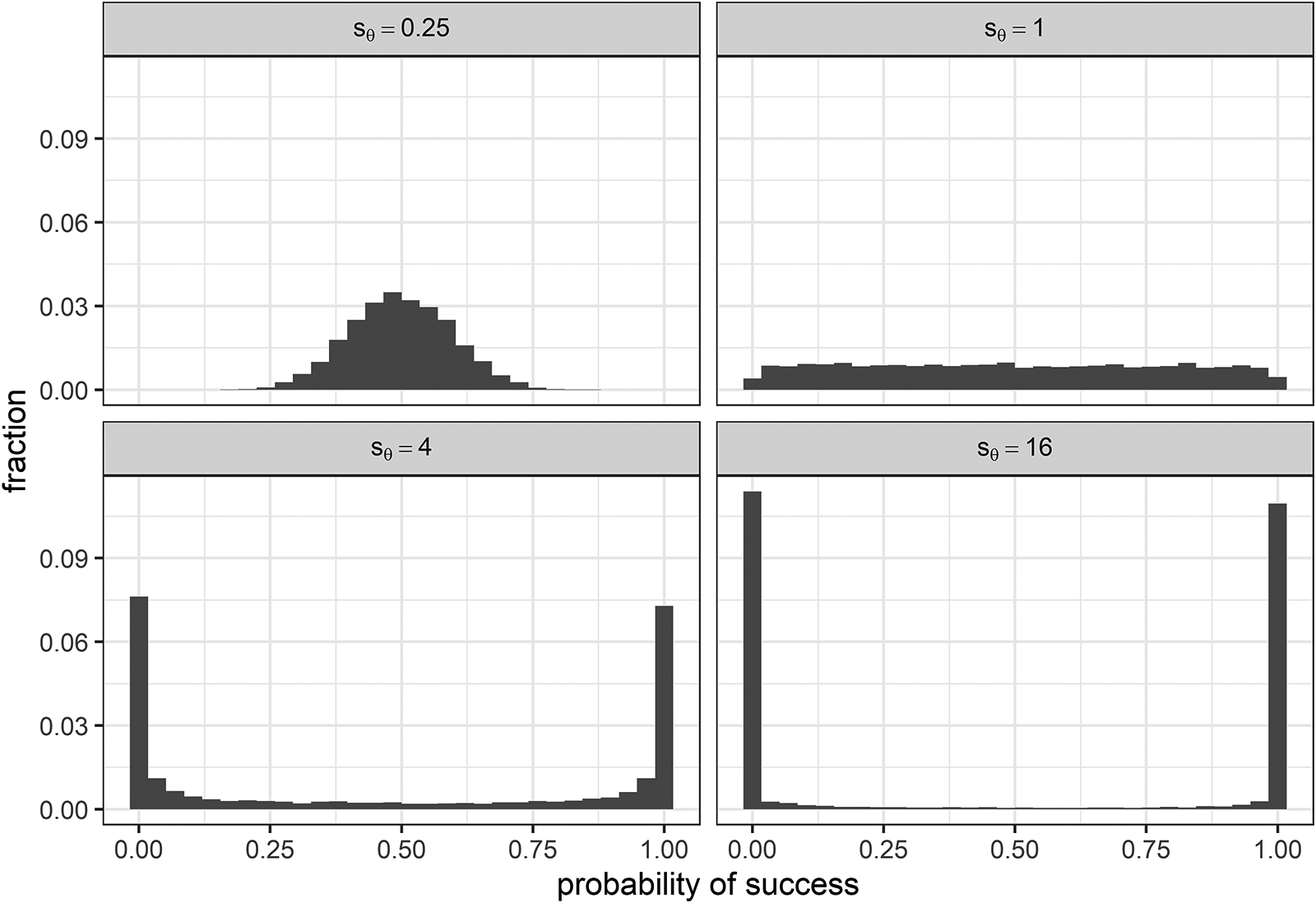
For λ, the probability of choosing the utility-maximizing is equal to  $(1+\exp(-\lambda |\Delta|))^{-1}$, where Δ is the difference in expected utility between the two lotteries. We can use this to explore the implications of different values of λ for a given lottery pair. In Figure 2 I plot this probability as a function of λ for a choice between $30 for sure, and a 50-50 mix between $10 and $50. This Figure shows how the prediction changes with λ for three different values of r. Note that based on our calibrated prior for r, r = 0.27 (dotted line) is the prior mean, and
  $r=-0.09$ (solid line) and r = 0.63 (dashed line) are one prior standard deviation either side of this. Looking at the dotted line, which corresponds to our calibrated prior mean of r = 0.27, most of the plausible choice probabilities lie in the region
  $\lambda\in(10,100)$. That is for λ > 100 choices seem very precise, and for λ < 10 choices seem very noisy. Given our choice of a log-normal prior for λ, we can calibrate this prior to these endpoints so that the prior probability that
 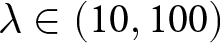 $\lambda\in(10,100)$ is (say) 95% as follows:
 \begin{equation*}
\begin{array}{ll}
\log 100 &=m_\lambda +1.96 s_\lambda\\
\log 10 &=m_\lambda -1.96 s_\lambda\\
\implies m_\lambda &\approx 3.45,\quad s_\lambda\approx 0.59
\end{array}
\end{equation*}
\begin{equation*}
\begin{array}{ll}
\log 100 &=m_\lambda +1.96 s_\lambda\\
\log 10 &=m_\lambda -1.96 s_\lambda\\
\implies m_\lambda &\approx 3.45,\quad s_\lambda\approx 0.59
\end{array}
\end{equation*} For perspective, this implies a prior mean of  $E(\lambda)=\exp(3.45+0.5\times 0.59^2)\approx 37$, which is shown as the vertical red line in Figure 2.
Probability of choosing the utility-maximizing lottery between (i) $30 for sure and (ii) a 50-50 mix of $10 and $50

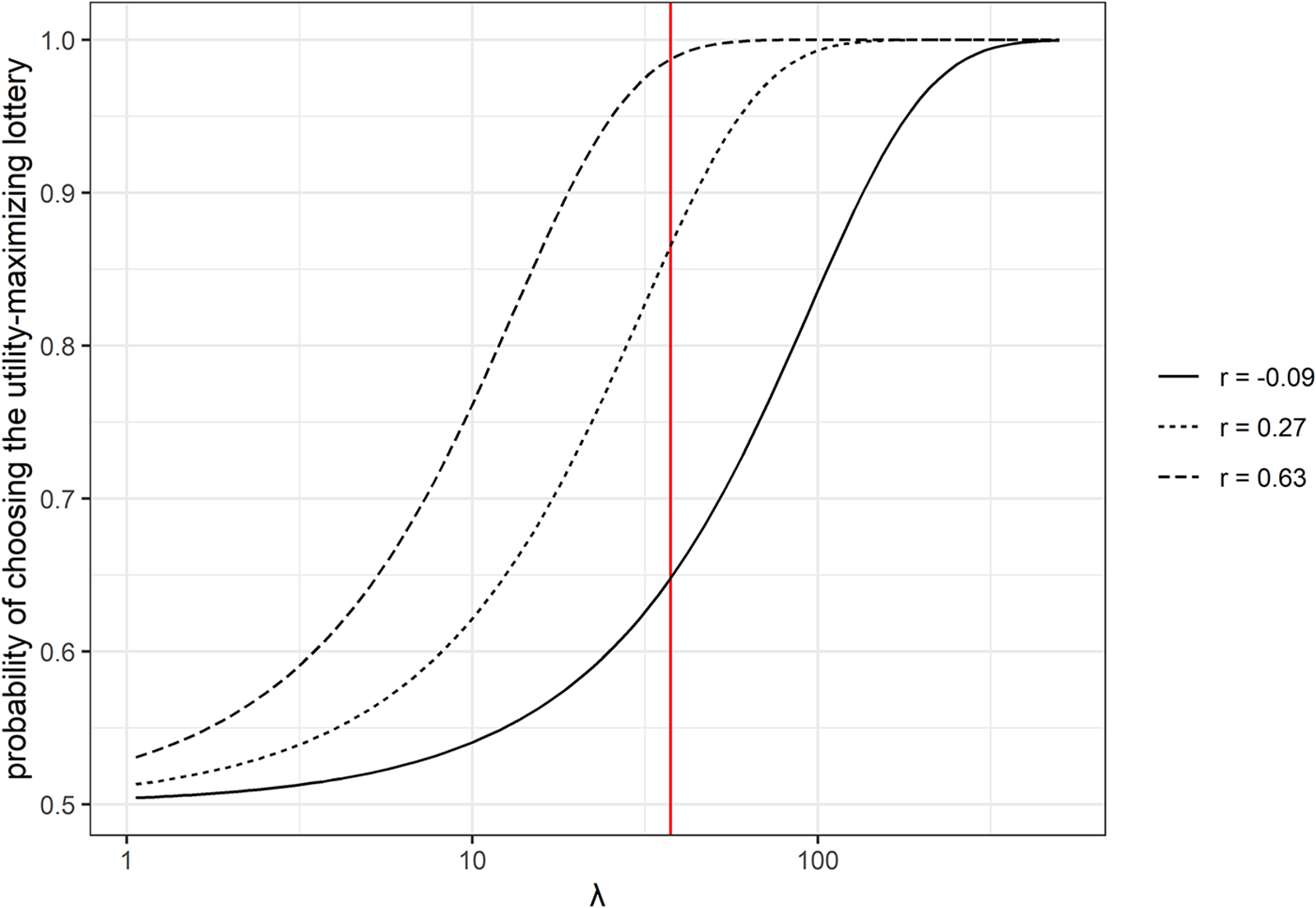
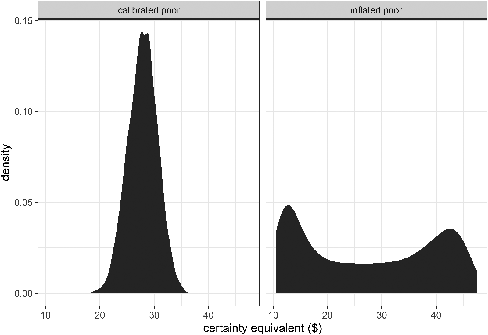
Even if we have a good understanding of how to interpret our parameters without transforming them into predictions or other quantities, investigating the implications of our prior on quantities of interest can be helpful. For example with an experiment investigating risk preferences like Harrison & Ng Reference Harrison and Ng(2016), we may be more interested in what our parameters imply about a certainty equivalent than on the parameters themselves. To this end, in Figure 3 I plot the prior distribution of the certainty equivalent of a lottery that is a 50-50 mix of $10 and $50. I do this for the calibrated prior (left panel) and an “inflated” prior (right panel), where I increase the prior standard deviations by a factor of 10 to demonstrate the effect of a highly diffuse prior. For the inflated prior, the certainty equivalent’s prior distribution has modes close to the endpoints of their allowable values ($10 and $50). This may not be a desirable implication of our prior, so checking for these implications is important.
Prior distributions of a certainty equivalent for the calibrated prior and a prior inflating the standard deviations by a factor of 10

3.3. Priors guided by the performance of our estimator
We should also evaluate our prior, coupled with the rest of our model and experiment design, on how well it achieves our inferential goal. Since our structural model includes a likelihood, we can simulate data from our experiment for known parameter values, and since we also have a prior, we can also simulate data from our experiment consistent with our prior beliefs. It is therefore possible, before running the experiment, to investigate the sampling properties of our estimator. This might not only identify problems with our prior if they exist, but also provides us with an opportunity to re-design the experiment if this exercise reveals that we are not estimating our desired quantities as well as we would like.
To demonstrate this in a Monte Carlo exercise, I draw 1,000 sets of parameters from the calibrated prior. For each of these draws, I then simulate a dataset using these parameters and estimate the model four times: (i) with the calibrated prior, (ii) with both prior standard deviations inflated by a factor of 2, (iii) with both prior standard deviations inflated by a factor of 8, and (iv) using maximum likelihood estimation. The root mean squared error of posterior means of the model’s parameters and the certainty equivalent are shown in Table 2.Footnote 10 The maximum likelihood estimator (right-most column) performs by far the worst of the five estimators under consideration, followed by the estimator using the most inflated prior. The Bayesian estimator with the calibrated prior estimates these quantities with smaller error.
Root mean squared error of posterior mean estimates and maximum likelihood estimates. The certainty equivalent is for a lottery that mixes 50-50 over prizes  $ \$ 10$ and
  $ \$ 50$

Figure 4 shows the estimated certainty equivalents against their true values. A model that recovers its parameters well will have posterior means (dots) close to the 45∘ line (red dashed line). A good example of this is the top-left panel of this Figure, which shows the results when using the calibrated prior. Estimates are slightly pulled toward to prior mean, which is to be expected for a Bayesian estimator. Looking at the bottom two panels, we can see that posterior estimates are more noisy (posterior means are more spread out vertically), less precise (credible regions are larger), and exhibit more bias (the smoothed means are further away from the 45∘ line).
Simulated estimates of a certainty equivalent (vertical axis) against their true values (horizontal axis) for various prior specifications and maximum likelihood estimates. Dots show posterior means, vertical lines show a 50% Bayesian credible region (25th-75th percentile). No expression of uncertainty is shown for the maximum likelihood estimates. The red dashed line is a 45∘ line. The blue curve shows a smoothed mean of the posterior means
4. Conclusion
This paper provides guidance for choosing priors when estimating structural models in economic experiments using Bayesian techniques. The choice of prior is not inconsequential for sample sizes used in typical economic experiments, and so care must be taken to calibrate this prior so that (i) it reflects our underlying knowledge of our parameters and other quantities before we observe the data, and (ii) we are satisfied with our model’s ability to estimate these parameters from our experiment. However one should not see this as always being in favor of highly informative priors: the exercise of prior calibration should help us with expressing our increased uncertainty without implying implausible predictions.
Prior calibration plays (at least) two useful functions. Firstly, we formally state and justify what we believe is the economically meaningful range of our models’ parameters. Secondly, through simulating parameters, then data from the calibrated prior, we explore the implications of our estimators for datasets which are hopefully similar to those we will see in our experiment. In doing so, we are able to assess our experiment’s ability to provide us with data that will answer our research question, and whether we should modify our design before collecting data.
This paper focuses on estimating models of behavior at the individual participant level. However the techniques it develops need not be limited to these applications. In particular, when estimating models that aggregate information from more than one individual, such as hierarchical models, the econometrician must choose priors over the model’s population-level “hyperparameters”, rather than the individual-level parameters.Footnote 11 Highly diffuse priors on these hyperparameters can also imply implausible prior distributions of individual-level parameters and the quantities of interest that can be derived from them. Hierarchical models estimated in such studies provide us with suggestions about what reasonable priors are for individual-level parameters. Using posterior mean estimates from Gao et al. Reference Gao, Harrison and Tchernis(2020) suggests that  $r\sim N(0.338,0.268^2)$ could be an appropriate prior for the CRRA parameter r.Footnote 12 This is not too dissimilar from the prior
  $r\sim N(0.27,0.36^2)$ I calibrated to Holt & Laury Reference Holt and Laury(2002), and is in fact more “informative”.
Supplementary material
The supplementary material for this article can be found at https://doi.org/10.1017/esa.2025.6.
Competing interests
The author declares no conflicts of interest.


 Open access