2. Experimental set-up and flow characteristics

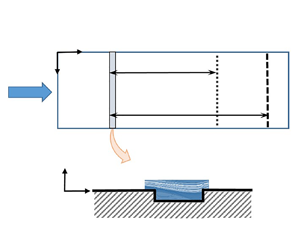
The flow field used for this investigation is based on a typical airfoil pressure distribution, with a favourable pressure gradient near the leading edge followed by a mild adverse pressure gradient downstream. To enable a systematic investigation of many gap geometries, the measurements are conducted on a flat plate with the pressure gradient imposed by contouring the opposing wind-tunnel wall. Figure 1 provides a schematic description of the test set-up, showing a top-down view on the test plate with a rectangular gap running spanwise across the plate surface. The gap is characterized by its streamwise position $x_G$ (measured from the plate leading edge to the gap leading edge), width $w$ and depth $d$. The gaps are created by interchangeable inserts, resulting in sharp-corner rectangular cavities. Measurements show the width and depth are uniform across the span to within $\pm$0.1 mm and $\pm$0.01 mm, respectively.

Figure 1. Schematic showing top-down view of the test model, parameters contributing to the normalized transition length $\xi$ and gap characteristics.

The effect of the gap on transition is primarily assessed by the change in transition location $x_T$ relative to the smooth-surface transition location $x_{T0}$. This transition movement is expressed in terms of the normalized transition length $\xi = (x_T - x_G )/( x_{T0} - x_G )$.

The experiments are conducted in the T-324 low-turbulence wind tunnel at the Khristianovich Institute of Theoretical and Applied Mechanics. Two test plates are used, each is 2050 mm long and 996 mm wide spanning the width of the test section. A trailing-edge flap is used to position the stagnation line on the upper quarter of a semi-circular plate leading edge. Measured coefficient of pressure C_p distributions are given in figure  2 for both gap positions that are considered, $x_G =127$ and $x_G =450$ mm. The small differences in the pressure (visible on the expanded scale of the inset) are the result of using different leading-edge lengths to position the gap, and some small inaccuracies in the plate mounting. These differences in $Cp$ are accounted for in the analysis of § 3. The first measured points downstream of $x \approx 0$ show there is a small suction peak on the upper (working) surface of the plate. Apart from the local variation at the leading edge, the upstream pressure distribution has a favourable gradient up to approximately $x \approx 200$ mm. This is followed by a mild adverse gradient that extends downstream beyond the transition location. Thus, the gap at $x_G =127$ mm is in a favourable pressure gradient, and the gap at $x_G = 450$ mm is in an adverse pressure gradient.

Figure 2. Pressure distribution, $Cp$, for the $x_G =$ 127 and $x_G=$ 450 mm configurations.

The study focuses on low Mach numbers, $M< 0.1$, similar to earlier investigations on steps (Crouch & Kosorygin, Reference Crouch and Kosorygin2020). Measurements are conducted using four different flow velocities, referred to as U18, U20, U22 and U27, with actual velocities, 18.3, 20.6, 22.6 and 27.5 m s$^{-1}$, respectively. For this range of tunnel velocities, the free-stream turbulence (measured with the model in place) varies between $Tu=0.028\,\%$ and $Tu=0.039\,\%$ (bandwidth $2\text {--}4 \times 10^3$ Hz). A representative turbulence spectrum for this facility is provided in Reference Crouch, Ng, Kachanov, Borodulin and IvanovCrouch, Ng, Kachanov, Borodulin, and Ivanov (Reference Crouch, Ng, Kachanov, Borodulin and Ivanov2015). Average values (over multiple tests entries) for the unit Reynolds number and the displacement thickness at the gap locations are provided in table 1. These displacement thickness values are from measurements on the smooth surface that are used to non-dimensionalize the gap width and depth in the results below.

Table 1. Overview of test parameters.

The transition location is determined using a 1 mm diameter Preston tube to measure the total pressure near the plate surface, as described in the earlier study on surface-step effects (Reference Crouch and KosoryginCrouch & Kosorygin, 2020). The transition onset is here defined based on the mean-flow profile rather than the unsteady fluctuations, since the mean flow is the essential quantity for most applications. The dynamic pressure drops with increasing $x$ distance, due to viscous thickening of the boundary layer. At the onset of transition, the dynamic pressure begins to rise – similar to the friction coefficient $C_f$. The transition-onset location $x_T$ is estimated based on the minimum in the dynamic pressure. Repeat runs (between 10 to 20 cases for each of the smooth-surface reference conditions) show the estimated transition location varies with a standard deviation of approximately $\pm$15 mm. This variation includes flow-condition uncertainty as well as transition-measurement uncertainty. A direct determination of the transition-measurement uncertainty based on various fits through the data gives an estimated value of ${\rm \Delta} x_T \pm 10$ mm.

3. Linear stability analysis

Linear stability analysis is used to assess the effects of the gaps on the transition location. The experimental $Cp$ distributions from figure 2 are used to create edge conditions for calculating the boundary-layer flow for the stability analysis. Earlier studies have shown very good agreement between the measured and calculated mean profiles for this flow (Reference Kosorygin, Crouch, Ng and SchlatterKosorygin, Crouch, & Ng, 2010). Calculated values for $\delta ^*$ are within $\pm$0.01 mm of the experimental values of table 1. Following quasi-parallel theory, the amplification of TS instabilities is described by the spatial growth rate $\gamma (x; \omega, \beta )$, which is determined from the Orr–Sommerfeld equation for the frequency $\omega = 2 {\rm \pi}f$ and spanwise wavenumber $\beta = 2 {\rm \pi}/ \lambda _z$. A physical mode of instability with fixed frequency $f$ and spanwise wavelength $\lambda _z$ can be characterized by its amplification factor $m$, defined as the natural log of the amplitude ratio

(3.1)\begin{equation} m(x; \omega , \beta ) = \ln \left( \frac{A(x; \omega , \beta ) }{A_0 ( \omega , \beta )} \right) = \int_{x_0}^{x} \gamma (s; \omega , \beta ),{\rm d} s. \end{equation}

In the $e^N$ method, when the amplification factor for any given mode reaches a critical value $N$, transition is assumed to occur. This is tracked using the $n$-factor envelope of the physical growth curves,

(3.2)\begin{equation} n(x) = \max_{\omega} \max_{\beta} m(x; \omega , \beta ), \end{equation}

such that the transition location is estimated from the occurrence where $n$ reaches the critical value $N$.

In the variable $N$-factor approach, the threshold value $N$ is defined as a function of key parameters that can alter the linear amplitude of the instability through either receptivity or enhanced amplification (Reference Crouch and SherwinCrouch, 2021). This is equivalent to a linear-amplitude method that correlates the transition onset to the amplitude $A$ reaching some threshold value $A_T$. Rather than tracking an increase in the physical amplitude relative to $A_T$, the variable $N$-factor approach tracks a reduction in the critical value $N$ relative to a reference condition with $N_0$, $N= N_0 - {\rm \Delta} N$ (Reference Crouch and SherwinCrouch, 2021). The amplification factors $m$ or $n$ are calculated the same as for the standard $e^N$ method, with only the critical value $N$ changing as a function of receptivity or growth modifiers.

Amplification curves $m(x; \omega, \beta )$ for the $U18$ $x_G = 450$ mm configuration are shown in figure 3 for a frequency range $100$ Hz $\leq f \leq 520$ Hz. For these conditions, the smooth surface transition location is $x_{T0} = 980$ mm. The dominant mode at this location is highlighted in red, and corresponds to $f=180$ Hz. This yields a non-dimensional frequency $F = 10^6 \omega \nu / U^2 =51$. These growth characteristics are consistent with TS instability being the mechanism for transition. As is typical for an airfoil pressure distribution, the same physical mode is dominant over an extended streamwise distance. Thus, any modest movement in transition is likely to be linked to a change in amplitude for this mode.

Figure 3. Instability amplification factors $m(x; \omega, \beta )$, for different frequencies $f =\omega / \textit{2} {\rm \pi}$, based on the $x_G=$ 450 mm $Cp$ distribution and the U18 velocity. The thick red line corresponds to $f=$ 180 Hz.

The $n$-factor envelopes for the various conditions tested are given in figure 4 (focusing on the frequency range relevant to transition). The solid red line in figure 4 is the envelope corresponding to figure 3. The dashed lines show the envelopes for the $x_G = 127$ mm configuration. The small differences in pressure distribution shown in figure 2 result in a slight destabilization of the $x_G=127$ mm configuration compared with $x_G=450$ mm. However, the $n$-factor differences between the two configurations remain less than $0.3$. For all flow conditions considered, the gap at $x_G = 127$ mm is upstream of the instability neutral point, and the gap at $x_G =450$ mm is downstream of the instability neutral point for all modes influencing transition.

Figure 4. Instability amplification-factor envelopes $n(x)$, for different velocities $U$, based on the $x_G =$ 127 mm and $x_G=$ 450 mm $Cp$ distributions.

4. Experimental results on gap effects

For the reference conditions on a smooth plate, the transition location varies between $780\,{\rm mm} \leq x_{T0} \leq 980\,{\rm mm}$, changing primarily due to velocity. The associated smooth-plate transition $N$-factors are between $8.9$ and $9.8$, and dominated by two-dimensional modes. The transition location varies weakly in the spanwise direction, with ${\rm \Delta} x_T \pm 5$ mm over ${\rm \Delta} z = 100$ mm, both for the smooth surface and with the spanwise-uniform gaps. The experimental data consider a wide range of gap widths and depths – expressed non-dimensionally by $0 < w / \delta ^* < 110$ and $0 < d / \delta ^* < 11$. Uncertainties in these non-dimensional values are dominated by the small $\delta ^*$ variations, and are estimated to be less than $\pm 2\,\%$. For the smallest values of $w$ and $d$, the uncertainties are set by the gap-measurement uncertainties of $\pm$0.1 and $\pm$0.01 mm, respectively.

A scatter plot of the various test points is given in figure 5. Each symbol represents a transition measurement, and the different symbol types show the normalized transition length $\xi$. The small black open symbols correspond to large transition lengths $\xi > 90\,\%$, with relatively little movement of transition due to the gap. The intermediate black open symbols correspond to $\xi$ between 50 % and 90 %. The large red open symbols (for larger $w / \delta ^*$ values) are associated with larger movements of transition toward the gap, with $\xi$ between 10 % and 50 %. Finally, the solid red symbols show conditions resulting in transition near, or at, the gap location. These cases of abrupt transition at the gap location appear to be the result of a bypass mechanism, not related to TS instability. For larger values of $d/ \delta ^*$, the experimental data suggest a threshold value of $w / \delta ^* > 19$ for bypass transition. The dashed lines in figure 5 (for $d / \delta ^* =2$ and $w/ \delta ^* =18$) are taken from Reference Beguet, Perraud, Forte and BrazierBeguet et al. (Reference Beguet, Perraud, Forte and Brazier2017). These lines show the boundary for gap characteristics leading to rapid transition at the gap location based on several experiments conducted at ONERA. The boundary between the open symbols and the solid symbols is in good agreement with these earlier experiments. To compare with the $Re_w =15\,000$ threshold criterion from Reference Nenni and GluyasNenni and Gluyas (Reference Nenni and Gluyas1966), we recast the observed threshold boundary at $w/ \delta ^* =19$ into $Re_w$ values. This yields a range of $Re_w$ values from approximately 12 000 up to approximately 33 000. While $Re_w = 15\,000$ is within this range, it does not provide a clear demarcation of the threshold. Note that the conditions studied in the work of Reference Zahn and RistZahn and Rist (Reference Zahn and Rist2016) are along the $d / \delta ^*$ axis, outside the range of the current results.

Figure 5. Scatter plot of experimental points in terms of gap width and gap depth, with symbols corresponding to the transition length $\xi$. (a) Full data set (both $x_G =$127 and $x_G=$ 450 mm), with dashed line showing the threshold boundary for bypass from Reference Beguet, Perraud, Forte and BrazierBeguet et al. (Reference Beguet, Perraud, Forte and Brazier2017), (b) Expanded view for smaller values of width and depth.

Figure 5(b) provides an expanded view of the results for smaller values of $w/ \delta ^*$ and $d/ \delta ^*$. For $d/ \delta ^* < 3.7$, the boundary for bypass transition shifts toward larger $w/ \delta ^*$. At $d/ \delta ^* \approx 1.8$, the threshold value for bypass is estimated as $w/ \delta ^* \approx 35$ based on the trend below $d/ \delta ^* \approx 3.7$. Values of $d/ \delta ^*$ below $1.8$ do not result in bypass transition, even for large values of $w/ \delta ^*$.

Streamwise disturbance amplitudes measured for three different flow conditions from figure 5 are presented in figure 6. The gap position is shown schematically on the $x$ axis. The amplitudes are measured using a hot-wire at a varying height above the surface corresponding to $U/Ue_G = 0.4$, where $U$ is the boundary-layer mean velocity and $Ue_G$ is the edge velocity measured at the gap location $x_G =450$ mm. The root-mean-square amplitude is obtained by band pass filtering the $u'$ signal over a narrow frequency band of $1.5\,\%$ of the central value. The target frequencies are selected to match the dominant frequency just prior to breakdown, as observed in measured spectra. In all cases, transition occurs due to ‘natural’ background forcing, without any direct excitation.

Figure 6. Streamwise variation of the disturbance amplitude for four different conditions with $x_G=\textit{450}$ mm: smooth plate at U18, $f=\textit{178}$ Hz; case A($w/ \delta ^* =\textit{27}$, $d/ \delta ^* =\textit{2.60}$) at U18, $f=\textit{175}$ Hz; case B($w/ \delta ^* =\textit{18}$, $d/ \delta ^* =\textit{3.45}$) at U18, $f=\textit{183}$ Hz; case C($w/ \delta ^* =\textit{20}$, $d/ \delta ^* =\textit{3.83}$) at U22, $f=\textit{830}$ Hz. Symbols are measurements and thin lines are linear theory for U18. Rectangles show the measured transition locations.

The black circular symbols are for measurements on the smooth plate for the U18 condition, and are provided for reference. The disturbance frequency for this case is $178$ Hz, which corresponds to a non-dimensional frequency of $F=10^6 \times 2 {\rm \pi}f \nu /U^2 = 53$. The solid line running through the data is derived from the calculated growth factor $m$ from (3.1) for $f=180$ Hz. The amplitude variation is given by $e^m$, and the initial amplitude $A_0$ is chosen to provide a good fit to the data in the neighbourhood of $x \approx 700$ mm. As shown in figure 3, this mode is predicted to be dominant at transition. This overall agreement with the quasi-parallel theory suggests that the non-parallel effects are small over this part of the amplification curve. The black rectangle at $x=980$ mm shows the measured transition location for this smooth-plate condition, and the associated linear threshold amplitude at transition is approximately 0.5 %.

The three amplitude curves identified as A, B and C are measured in the presence of surface gaps at $x_G=450$ mm. For cases A ($w/ \delta ^* =27$, $d/ \delta ^* =2.6$) and B ($w/ \delta ^* =18$, $d/ \delta ^* =3.45$), the free-stream conditions are the same as for the smooth-surface reference case, U18. Case C ($w/ \delta ^* =20$, $d/ \delta ^* =3.83$) is measured at condition U22. The measured frequency for cases A and B is $f=175$ and $f=183$ Hz, respectively. These are essentially the same as the smooth-plate frequency. The calculated linear-amplitude curve for $f=180$ Hz is overlaid on the experimental data for these cases. Similar to the smooth-plate comparison, the initial amplitude level was chosen to provide a match to the data in the neighbourhood of $x \approx 700$ mm. The good agreement between theory and experiment for the pre-transition amplitude variation shows that the primary effect of the gap is to locally destabilize the TS wave, resulting in a larger amplitude. Assuming the same linear threshold amplitude for transition as for the smooth plate 0.5 % (using the current $u'$ amplitude definition), the shifted linear-amplitude curves for A and B provide a good prediction for the transition onset as shown by the rectangles for these cases. This provides support for using a linear-amplitude method, or the simplified variant of a variable $N$-factor method, for predicting the transition movement due to gaps.

The amplitude variation for case C is qualitatively different from cases A and B. The amplification at the gap location is much greater, and this leads to a more rapid transition – essentially at the gap location. In this case, there is no sign of any TS-wave growth. In addition, the frequency for case C is $f=830$ Hz (or $F=163$), which is well outside the expected range for TS-wave transition. This case can be characterized as a bypass to the underlying linear transition mechanism. This supports the observation that the threshold boundary in figure 5 is associated with bypass transition. Further evidence for this is provided by the recent global stability analysis of Reference Mathias and MedeirosMathias and Medeiros (Reference Mathias and Medeiros2019).

5. Analysis of gap effects for TS transition

Linear stability analysis and the variable $N$-factor formulation are used to investigate the linkage between the gap effects on TS waves and the observed transition movement presented in figure 5. For a given gap and flow condition, a smooth-surface amplification envelope from figure 4 is used to determine the critical $N$-factor $N$ at the measured transition location $x_T$. For the same flow condition, the smooth-surface transition location $x_{T0}$ is used to determine the reference $N$-factor $N_0$. This provides a ${\rm \Delta} N = N_0 - N$ as a function of the gap characteristics $w/ \delta ^*$, $d/ \delta ^*$.

There are two primary factors contributing to the uncertainty in the calculated ${\rm \Delta} N$. The first is the uncertainty in the measured transition location $x_T$ or $x_{T0}$, which, as noted above, is $\pm$10 mm. Using the steepest envelope curve from figure 4, this translates to an $N$-factor uncertainty of $\pm$0.17. The other source of uncertainty is a $3 \times (10)^4\,{\rm m}^{-1}$ standard deviation in unit Reynolds number for the range of test points corresponding to a given test condition in table 1. This results in an $N$-factor uncertainty of ${\pm }0.12$. The cumulative uncertainty for a given $N$-factor calculation is ${\pm }0.21$, and the associated uncertainty for ${\rm \Delta} N$ is ${\pm }0.3$. Note that a larger transition uncertainty of ${\pm }15$ mm would result in a cumulative ${\rm \Delta} N$ uncertainty of ${\pm }0.4$.

Figure 7 shows the calculated ${\rm \Delta} N$ for all of the gap measurements with $x_G =450$ mm as a function of the gap depth and gap width. The different symbols correspond to the gap-width bins that are used to organize the data. The solid line in figure 7(a) shows the ${\rm \Delta} N =4.4 d/ \delta ^*$ variation for a backward-facing step from Reference Crouch, Kosorygin and NgCrouch et al. (Reference Crouch, Kosorygin and Ng2006). All of the data are bounded by the backward-facing step trend line, showing that the gap effects on TS waves are no worse than a backward-facing step of height $d / \delta ^*$. The results show that the ${\rm \Delta} N$ initially increases with $d/ \delta ^*$ similar to a backward-facing step but then ${\rm \Delta} N$ plateaus to a nearly constant value, which depends on the gap width. The points in the grey band between $6 < {\rm \Delta} N <7.5$ correspond to transition occurring at the gap location, and are likely the result of bypass transition as discussed above.

Figure 7. Variation of ${\rm \Delta} N$ as a function of (a) gap depth and (b) gap width for gaps at $x_G=\textit{450}$ mm, in an adverse pressure gradient. Dashed lines show the mean slope ($\textit{0.1} w/ \delta ^*$) and $\pm$ one standard deviation.

Figure 7(b) shows the same data plotted as a function of gap width $w/ \delta ^*$. The thick dashed line through the data ($0.1 w/ \delta ^*$) shows the mean value calculated from ${\rm \Delta} N /(w/ \delta ^*)$ for data in the range $7 \leq w/ \delta ^* \leq 30$; smaller values of $w/ \delta ^*$ overly amplify data scatter, and larger values are potentially influenced by bypass transition. The thin dashed lines in figure 7(b) show the mean slope plus or minus one standard deviation. The mean plus one standard deviation provides a good bounding curve for the data.

The non-bypass results of figure 7 show two distinct trends in the ${\rm \Delta} N$ variation. For small values of $d/ \delta ^*$, the ${\rm \Delta} N$ varies with $d/ \delta ^*$ similar to a backward-facing step. This variation is independent of the gap width $w/ \delta ^*$, as long as the width is sufficiently large compared with the depth. Qualitatively, this is a shallow gap that is dominated by the upstream backward-facing step, with minimal influence from the downstream forward-facing step. For larger values of $d/ \delta ^*$, the ${\rm \Delta} N$ approaches a constant value that depends on the gap width. In this deep-gap limiting case, the value of ${\rm \Delta} N$ is independent of the depth.

Based on the slope for the average $w/ \delta ^*$ dependence from figure 7(b), the overall ${\rm \Delta} N$ variation is given by

(5.1)\begin{equation} {\rm \Delta} N = \left\{\begin{array}{ll} 4.4 d/ \delta ^ * & : d/w \leq 0.023 \\ 0.1 w/ \delta ^ * & : d/w > 0.023. \end{array}\right. \end{equation}

The boundary between the shallow-gap and deep-gap behaviour is determined by equating ${\rm \Delta} N$ from the two expressions. A deep-gap behaviour is also seen in the study of Reference Beguet, Perraud, Forte and BrazierBeguet et al. (Reference Beguet, Perraud, Forte and Brazier2017) based on the change in the far-field growth factor ${\rm \Delta} n_{far}$. When applied to the current test conditions for $x_G=450$ mm, their ${\rm \Delta} n_{far}$ variation slopes are between $0.07 w/ \delta ^*$ and $0.08 w/ \delta ^*$, which is at the lower end of the range of slopes from figure 7(b).

The limiting behaviours of (5.1) are shown schematically by the solid and dashed straight lines in figure 8. A simple model that smoothly transitions between the shallow-gap and deep-gap behaviour, based on the average slope of ${\rm \Delta} N$ versus $w/ \delta ^*$, is

(5.2)\begin{equation} {\rm \Delta} N \approx 0.1 w/ \delta^ * \tanh \left(\frac{44d}{w}\right). \end{equation}

This model variation is shown by the red dashed curve in figure 8, in relation to the limiting behaviours.

Figure 8. Schematic showing the ${\rm \Delta} N$ variation with gap depth for a fixed gap width. For shallow gaps the ${\rm \Delta} N$ varies like a backward-facing step, and for deep gaps the ${\rm \Delta} N$ takes on a constant value that depends on the width.

Due to the data scatter of figure 7, the $d/w$ value differentiating shallow-gap behaviour from deep-gap behaviour is not well defined, but is in the range $0.017 < d/w < 0.028$ (or, $36 < w/d < 59$), based on using the slopes of the two thin dashed lines from figure 7(b). To conservatively account for this data scatter, an alternative expression for ${\rm \Delta} N$ is given by

(5.3)\begin{equation} {\rm \Delta} N \approx 0.122 w/ \delta^ * \tanh \left(\frac{36d}{w}\right). \end{equation}

This provides an approximate bounding curve for the results (Crouch, Kosorygin, & Sutanto, Reference Crouch, Kosorygin and Sutanto2020) – essentially one sigma above the average in figure 7(b). This study did not include detailed investigation of the gap flow, but the shallow-gap/deep-gap boundary is thought to be linked to the flow-reattachment distance within the gap. For the shallow gap, the recirculation length is set by the gap depth, but for the deep gap it is limited by the gap width.

Comparisons between the model expressions of (5.2) and (5.3) and the experimental data are provided in figure 9, which essentially combines figures 7 and 8. Similar to figure 7, the grey bands at larger ${\rm \Delta} N$ show points that have transition at the gap location, and are likely bypass transition. The thicker dashed lines are for the average behaviour of (5.2), and the thin dashed lines are for the bounding case of (5.3). Figure 9(a) shows the results for $x_G=450$ mm, with the gap in the adverse pressure gradient. This is from the same data set shown in figure 7, and used to develop the model. Figure 9(b) shows results for $x_G=127$ mm, with the gap in the favourable pressure gradient. These data also show good agreement with the model, although biased towards smaller ${\rm \Delta} N$ values, similar to earlier step results (Reference Crouch, Kosorygin and NgCrouch et al., 2006). Even though the TS-instabilities are nominally damped at $x=127$ mm, this location is relatively close to the neutral points for the critical modes. In this case, the destabilizing effects of the gaps are still significant.

Figure 9. Variation of ${\rm \Delta} N$ with gap depth for different values of gap width for both (a) $x_G=\textit{450}$ mm and (b) $x_G =\textit{127}$ mm. Model predictions from (5.2), thick dash; model predictions from (5.3), thin dash; and experimental results, symbols.

To provide a general characterization of the gap effects, the model of (5.2) is used to recast the transition length results of figure 5 into ${\rm \Delta} N$ contours. Figure 10 shows the ${\rm \Delta} N$ resulting from different gap widths and depths. The cross-hatch area shows the region where bypass transition occurs, which is independent of the TS-wave amplification.

1. (i) For gap depths greater than $d/ \delta ^* \approx 3.7$, bypass transition occurs for gap widths $w/ \delta ^* > 19$; for narrower widths, $w/ \delta ^* < 19$, the maximum ${\rm \Delta} N$ is less than 2. For this range of gap depths, the reduction in the critical $N$-factor results in a relatively small movement in transition compared with bypass.

2. (ii) For depths in the range $1.8 < d/ \delta ^* < 3.7$, the reduction in critical $N$-factor can be as large as 3.5.

3. (iii) For depths below $d/ \delta ^* \approx 1.8$, the transition movements result from changes in the TS-wave critical $N$-factor. In this range of depths, the transition movement is a function of both the gap width and depth.

Figure 10. The TS-wave ${\rm \Delta} N$ contours and bypass-transition region as a function of the gap width $w/ \delta ^*$ and depth $d/ \delta ^*$ based on low Mach number data ($M<\textit{0.1}$) for nominally two-dimensional boundary layers.