


Introduction
Terrestrial archives that can inform past environmental change are rare in Antarctica because < 1% of the Antarctic continent is ice free. The largest contiguous ice-free areas, the McMurdo Dry Valleys (MDVs), have probably remained ice free since the Miocene (Denton & Sugden Reference Denton and Sugden2005, Lewis et al. Reference Lewis, Marchant, Ashworth, Hemming and Machlus2007) and contain a rich geomorphological record. These valleys are characterized by a range of climatic zones that contain distinct landform assemblages (e.g. Marchant & Head Reference Marchant and Head2007) and have informed reconstructions of past cryospheric and environmental change over multimillion-year timescales (e.g. Sugden et al. Reference Sugden, Marchant, Potter, Souchez, Denton, Swisher and Tison1995, Marchant et al. Reference Marchant, Lewis, Phillips, Moore, Souchez and Denton2002, Swanger et al. Reference Swanger, Marchant, Kowalewski and Head2010, Reference Swanger, Marchant, Schaefer, Winckler and Head2011, Reference Swanger2017).
Ice-free valley systems that exist elsewhere in Antarctica also have potential as long-term geomorphological and palaeoenvironmental archives (e.g. Bockheim et al. Reference Bockheim, Wilson, Denton, Andersen and Stuiver1989, Hodgson et al. Reference Hodgson, Bentley, Schnabel, Cziferszky, Fretwell, Convey and Xu2012, Bibby et al. Reference Bibby, Putkonen, Morgan, Balco and Shuster2016). To realize this potential, it is essential that the relevant landforms be described and mapped so that process-form analogues can be identified and their palaeoenvironmental significance assessed. A geochronological framework can shed light on the potential length of the archive(s) as well as the timing of events and rates of processes: this allows relevant research questions to be developed for future work. The purpose of this paper is to describe a potentially valuable geomorphic record of past cryospheric change from ice-free valley systems within the Neptune Range of the Pensacola Mountains in the southern Weddell Sea sector of Antarctica (Fig. 1). We present initial geomorphological mapping and interpretation of the observed landforms with reference to potential analogues in the MDVs and other similar climatic settings. Preliminary geochronological data (10Be and 26Al exposure ages) are presented to demonstrate the potential length of the record preserved in the Neptune Range dry valley systems.
a. Location map showing the Weddell Sea Embayment (WSE) in the context of the Antarctic continent. EAIS = East Antarctic Ice Sheet; WAIS = West Antarctic Ice Sheet. b. Current ice-sheet configuration and location of the Pensacola Mountains in the WSE with measured flow velocities (Rignot et al. Reference Rignot, Mouginot and Scheuchl2011). AG = Academy Glacier; FIS = Foundation Ice Stream. c. Hill-shaded digital elevation model (Reference Elevation Model of Antarctica 8 m; Howat et al. Reference Howat, Porter, Smith, Noh and Morin2019) of the Neptune Range and main geographical features mentioned in the text.

Regional setting and wider significance
The Neptune Range is a massif within the Pensacola Mountains in the south-east portion of the Weddell Sea embayment (Fig. 1). The Pensacola Mountains are dominated by folded sandstones, mudstones, conglomerates and limestones, with minor igneous rocks exposed in their western part (Schmidt et al. Reference Schmidt, Williams and Nelson1978). The Neptune Range consists of the Washington Escarpment with associated ridges and valleys, the Iroquois Plateau, the Schmidt Hills and the Williams Hills. These latter two massifs are located on the eastern margin of the Foundation Ice Stream (FIS) and are separated from the Washington Escarpment by the ice-filled Roderick Valley. The Washington Escarpment trends north-west to south-east for > 100 km and, at its southern end, the Academy Glacier flows from the polar plateau and is confluent with the FIS. To the east of the Washington Escarpment the Iroquois Plateau comprises a large snowfield at an elevation of ~1400 m. Outlet glaciers from this snowfield overtop the Washington Escarpment in numerous places and flow west into Roderick Valley and, via Childs Glacier, into the trunk of the FIS (Fig. 1).
In several places, peaks on the Washington Escarpment are sufficiently high to prevent overriding by ice from the Iroquois Plateau (Fig. 2). In the lee of these highest peaks are several ice-free valleys that are blocked at their entrances by ice lobes that spill into the lower valleys from outlet glaciers flowing from the plateau towards Roderick Valley. There are two main areas where such valleys occur. First, in the lee of Nelson Peak (1605 m), Miller Valley and contiguous ice-free areas occupy ~20 km2 (Figs 2 & 3). Second, in the lee of the highest peak in the Neptune Range, Mount Hawkes (1975 m), are several unnamed valleys; the largest of these, unofficially termed South Hawkes Valley (SHV), Central Hawkes Valley (CHV) and North Hawkes Valley (NHV), have a combined area of ~40 km2 (Figs 2 & 4).
Location map of Washington Escarpment showing geographical features mentioned in the text, major ice-free areas, debris accumulations and sharp ridge crests indicative of alpine-like topography. White arrows denote main points where ice from Iroquois Plateau overtops the escarpment. Small, black arrows indicate lobes of ice that spill back to block the entrances of the valleys described in this study. Red dots indicate locations of cosmogenic nuclide samples from the crest of Elliot Ridge. Background imagery is the hill-shaded Reference Elevation Model of Antarctica 8 m digital elevation model (Howat et al. Reference Howat, Porter, Smith, Noh and Morin2019).

Overview satellite image of the Miller Valley area showing the main features mentioned in the text and the locations of cosmogenic nuclide samples. Insets denote locations of panels in Figs 9 & 19. Orange annotations indicate locations (squares) and directions (chevrons open in direction of view) of field photographs in Figs 13, 15 & 18 (satellite imagery - WorldView3 30 cm resolution - ©2018 DigitalGlobe, Inc., a Maxar company). Contours (50 m intervals) extracted from Reference Elevation Model of Antarctica 8 m digital elevation model (Howat et al. Reference Howat, Porter, Smith, Noh and Morin2019).

Overview satellite image of the Hawkes Valleys area showing the main features mentioned in the text. Insets denote locations of panels in Figs 9 & 19. Orange annotations indicate locations (squares) and directions (chevrons open in direction of view) of field photographs in Figs 13, 15 & 18 (satellite imagery - WorldView3 30 cm resolution - ©2018 DigitalGlobe, Inc., a Maxar company). Contours (50 m intervals) extracted from Reference Elevation Model of Antarctica 8 m digital elevation model (Howat et al. Reference Howat, Porter, Smith, Noh and Morin2019).

Modelled mean annual temperatures in this region are ~-27°C (Van Wessem et al. Reference Van Wessem, Reijmer, Morlighem, Mouginot, Rignot and Medley2014), and the Neptune Range is identified as an area of persistent wind scour, suggesting close to zero or slightly negative surface mass balance (Das et al. Reference Das, Bell, Scambos, Wolovick, Creyts and Studinger2013). Given the cold temperatures and low ice-surface velocities (<10 m yr-1; Rignot et al. Reference Rignot, Mouginot and Scheuchl2011), cold-based ice is expected to be widespread throughout the region. Noticeably, throughout the Neptune Range there are accumulations of supraglacial debris at numerous ice-marginal locations (Fig. 2). Current datasets do not fully resolve the bed topography within the Neptune Range, so it is not known whether ice within the ice-filled valleys is sufficiently thick to produce widespread pressure-induced melting and thus entrain significant amounts of debris at its bed by regelation processes. That said, ice acceleration where it spills over the Washington Escarpment could initiate erosion and subglacial debris entrainment due to localized development of strain heating (e.g. Clarke et al. Reference Clarke, Nitzan and Paterson1977, Evans & Rea Reference Evans, Rea and Evans2003). Additionally, cold-based ice can entrain some subglacial debris by interfacial water film regelation (e.g. Cuffey et al. Reference Cuffey, Conway, Gades, Hallet, Lorrain and Severinghaus2000) and debris can be sourced directly from rock fall onto the ice surface (e.g. Swanger et al. Reference Swanger, Marchant, Schaefer, Winckler and Head2011). Another common source of significant debris-rich ice facies in polar glacier margins is apron entrainment or sub-marginal freeze-on (net adfreezing), the latter being effective during periods of increased subglacial melting beneath thicker ice up-flow (cf. Shaw Reference Shaw1977, Evans Reference Evans1989, Reference Evans2009, Fitzsimons Reference Fitzsimons and Evans2003). Regardless of the precise origin, debris-rich ice facies may be thickened by fold/thrust stacking and compression (Hambrey & Fitzsimons Reference Hambrey and Fitzsimons2010), especially in areas where ablation is dominant (cf. blue ice moraines), as is expected in the Neptune Range.
Antarctic dry valleys such as the MDVs are controlled by wind-driven sublimation with valley floors at lower elevations than the surrounding ice. The Neptune Valleys differ because the valley floors rise to the east, away from the ice front (Figs 3 & 4). The existence of these valleys may, therefore, be due to the driving stress being insufficient to advance ice further into the valleys. Alternatively, the ice-front positions may be controlled by a combination of ice dynamics and ablation. Nevertheless, despite these potential differences and their relatively small size, the Neptune Valleys, because they are located at ~84°S, represent some of the southernmost ice-free valley systems in the Weddell Sea Embayment, and they contain a rich geomorphic record that has not, to our knowledge, been described or investigated in any detail (cf. Schmidt et al. Reference Schmidt, Williams and Nelson1978).
Miller Valley
Miller Valley (83.65°S, 55.21°W) is located to the north-west of Nelson Peak (Figs 2 & 3). Its eastern flank is formed by the upper portion of Brown Ridge, on the other side of which an outlet glacier overtops the Washington Escarpment. The upper headwall of Miller Valley is formed by Nelson Peak and its outliers. Miller Valley widens from its entrance at ~720 m above sea level (m a.s.l.) and is separated from a smaller unnamed valley by a spur that extends from Brown Ridge. To the south of the valley a cirque hosts a small glacier. The upper portion of Miller Valley rises steeply to another small upper cirque at ~1150 m a.s.l. beneath Nelson Peak. The floor of the valley is characterized by relatively coarse unconsolidated materials with no bedrock outcrops. Some bedrock does outcrop on spurs on the valley sides. Katabatic winds coming off the Iroquois Plateau are funnelled along Miller Valley to produce a blue ice ablation zone on the tongue of ice that spills into the valley entrance (Fig. 3).
Hawkes Valleys
The three main Hawkes Valleys (83.91°S, 56.24°W) are located towards the upper end of Jones Valley (Fig. 2), a major valley with an east-west ice gradient that connects ice spilling over from the Iroquois Plateau to the Roderick Valley. Both CHV and NHV have their entrances blocked by tongues of blue ice (~760 and ~800 m a.s.l., respectively) that spill back from ice in Jones Valley (Fig. 4). From the ice front, the valleys extend for ~4.0 km (CHV) and 2.5 km (NHV), with the upper valley floors at ~980 m a.s.l. (CHV) and 880 m a.s.l. (NHV) (Fig. 4). Both of these valleys are simple linear features with cirque-like headwalls and steep, rectilinear, debris-mantled slopes on both sides. They are ~1.2 and ~0.7 km wide, respectively. Their floors, as well as the vast majority of the valley sides, are characterized by unconsolidated material with very rare bedrock outcrops. SHV differs (Fig. 4), as its main ice-free area comprises a gently sloping bench that is ~500 m wide and situated ~150–200 m above a narrow, ~3 km-long, U-shaped valley. The western end of this valley is blocked by an ice tongue at ~650 m a.s.l.; however, at its eastern end an outlet glacier from the Iroquois Plateau overtops the escarpment, forming an ice fall ~280 m in height with its debris-covered terminus extending to within ~100 m of the ice tongue at the western valley entrance. To the north of this glacier are steep bedrock slopes and several cirques. The main ice-free bench slopes upwards from west to east (800–1140 m a.s.l.), and its southern flank is composed of steep debris-mantled slopes with two smaller re-entrant side valleys that host small glaciers.
Methods
Brief fieldwork (< 1 day) in the Miller Valley and NHV during the 2009–2010 field season highlighted the potential geomorphic record contained within these valleys and motivated subsequent mapping. CHV and SHV were not visited. Preliminary geomorphological mapping was undertaken from available aerial photographs and commercial satellite imagery (WorldView3 - 30 cm resolution; ©DigitalGlobe, Inc., a Maxar company) georeferenced to the newly available Reference Elevation Model of Antarctica (REMA) 8 m digital elevation model (DEM) of Howat et al. (Reference Howat, Porter, Smith, Noh and Morin2019). The higher-resolution 2 m REMA DEM was used to aid mapping of features; however, its spatial coverage within areas of high relief such as the Neptune Range is incomplete and thus it was not used for georeferencing. We endeavoured to map all glacial landforms; however, in some areas, particularly heavily shaded areas, we do not have sufficient information to state that an absence of mapped landforms equates to no landforms being present. The aforementioned fieldwork provided basic field observations and photographs that were used to aid identification and interpretation of relevant features. However, it did not provide time for sedimentological investigations and geophysical equipment was not available.
Schmidt et al. (Reference Schmidt, Williams and Nelson1978) noted erratics up to 1000 m above present-day ice and inferred that they were deposited by an ice sheet with a broadly similar configuration to present. Sampling for cosmogenic nuclide analysis (10Be and 26Al) was undertaken opportunistically during a wider sampling campaign (2009–2010) that aimed to constrain the thinning history of the last ice-sheet expansion in the Pensacola Mountains (Bentley et al. Reference Bentley, Hein, Sugden, Whitehouse, Shanks, Xu and Freeman2017). Samples were collected from two locations (Figs 2 & 3). First, in Miller Valley, ten samples were collected from distinct depositional features or from boulders located on a drift sheet surface to provide preliminary constraints on the geomorphological record (Fig. 5). Second, a further eight samples came from the crest of Elliot Ridge and are presented here as they provide some constraint on the wider ice-sheet history. The samples from Elliot Ridge consist of five erratic clasts and three bedrock samples (Fig. 5). Samples were taken whole or sampled from larger boulders and bedrock with a hammer and chisel. Topographical shielding was measured using an Abney level and compass. Sample location information is presented in Table I.
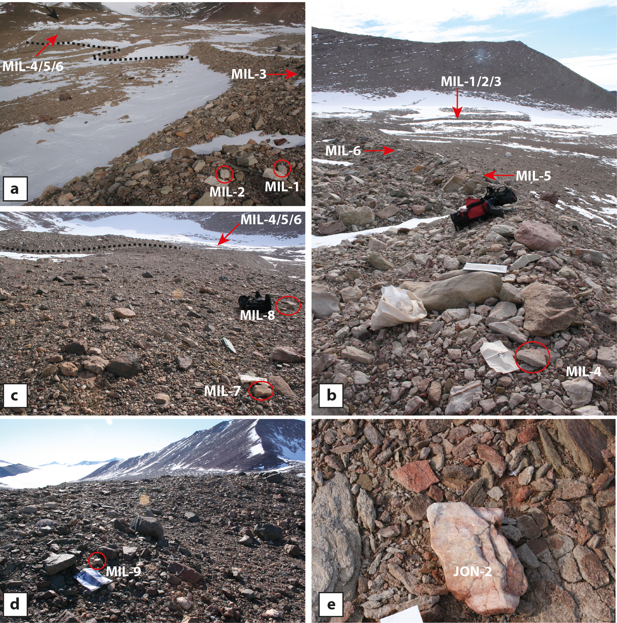
Field photographs showing the context of selected cosmogenic nuclide samples from Miller Valley (a.–d.) and Elliot Ridge (e.). a. Looking along the frontal slope (dashed line) of the large discrete debris accumulation (DDA) in Miller Valley from location of MIL-1/2/3. Location of MIL-4/5/6 is arrowed. b. Location of MIL-4/5/6 on the crest of the DDA, view is back towards the location of MIL-1/2/3 (arrowed). c. Looking back from the location of MIL-7/8, on an older moraine bench. Note crosscutting relationship of the DDA denoted by the dashed line. Also note the increased weathering compared to clasts in panels a. and c. Location of MIL-4/5/6 is arrowed. d. Location of sample MIL-9 (MIL-10 just out of view to the right). Note the increased degree of weathering of clasts. e. Sample JON-2 on the crest of Elliot Ridge. Note the distinct difference in appearance compared to the local bedrock.
Sample location, 10Be chemistry and accelerator mass spectrometry data.

a Samples spiked with Scharlau Be carrier (lot #10843401), 1000 mg l-1, density 1.02 g ml-1.
b Measured 10Be/9Be accelerator mass spectrometry ratios normalized to NIST SRM-4325 Be standard material with a nominal 10Be/9Be of 2.79 × 10⁻¹¹.
c Density-adjusted carrier additions to blanks ranged from 0.2364 to 0.2497 μg.
DD = decimal degrees.
Whole-rock samples were crushed and sieved to obtain the 250–710 μm fraction. Quartz purification and Be/Al extraction were undertaken at the University of Edinburgh's Cosmogenic Nuclide Laboratory following established methods (cf. Kohl & Nishiizumi Reference Kohl and Nishiizumi1992). 10Be/9Be and 26Al/27Al ratios were measured at the Scottish Universities Environmental Research Centre (SUERC) Accelerator Mass Spectrometry (AMS) Laboratory. Measurements are normalized to the NIST SRM-4325 Be standard material with a nominal 10Be/9Be of 2.79 × 10⁻¹¹ and the Purdue Z92-0222 Al standard material with a nominal 26Al/27Al of 4.11 × 10⁻¹¹. Be process blanks and samples were spiked with ~250 μg 9Be carrier (Scharlau Be carrier, 1000 mg l-1, density 1.02 g ml-1). Al blanks were spiked with ~1.5 mg 27Al carrier (Fischer Al carrier, 1000 ppm) and samples were spiked with up to ~1.5 mg 27Al carrier (the latter depending on the native Al content of the sample). Blanks range from 1.01 × 10⁻¹⁴ to 3.04 × 10⁻¹⁴ [10Be/9Be] and from 1.01 × 10⁻¹³ to 3.80 × 10⁻¹⁴ [26Al/27Al] (Tables I & II). Given the large measured concentrations, our results and interpretation are insensitive to blank corrections. Concentrations (Tables I & II) are corrected for process blanks; uncertainties include propagated AMS sample/lab blank uncertainty and a 2% carrier mass uncertainty.
26Al chemistry and accelerator mass spectrometry data.
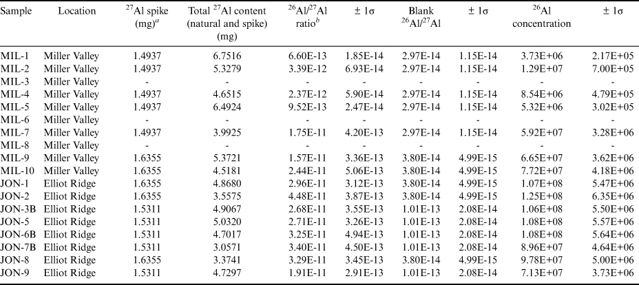
a Samples spiked with Fischer Al carrier, 1000 ppm.
b Measured 26Al/27Al accelerator mass spectrometry ratios normalized to Purdue Z92-0222 Al standard material with a nominal 26Al/27Al of 4.11 × 10⁻¹¹.
Apparent exposure ages (10Be and 26Al) were calculated online using the default production rate data-set and Lifton-Sato-Dunai (LSDn) scaling (Lifton et al. Reference Lifton, Sato and Dunai2014) within the exposure age calculator formerly known as the CRONUS-Earth online exposure age calculator, version 3 (https://sites.google.com/a/bgc.org/v3docs). Two-isotope plots were produced using iceTEA (Jones et al. Reference Jones, Small, Cahill, Bentley and Whitehouse2019). For brevity, only 10Be apparent exposure ages are quoted in the discussion. All apparent exposure ages and production rate-normalized 26Al/10Be ratios are presented in Table III. Ages were calculated assuming zero erosion and should thus be considered as minimum ages.
Apparent exposure ages and production rate-normalized 26Al/10Be ratios of all samples from Miller Valley and Elliot Ridge. Italicized ratios plot below the erosion island (Fig. 12).

DDA = discrete debris accumulation.
Interpretation of mapped geomorphological features
We first present our initial observations and interpretations of landforms in the Neptune Valleys before presenting the results of the preliminary geochronological analyses.
Large-scale bedrock (geo)morphology
The highest points on the Washington Escarpment crest, such as Mount Hawkes, Gambacorta Peak and Nelson Peak, have alpine forms with pyramidal peaks and intervening arêtes (Fig. 2). Lower sections of the escarpment are generally overridden by ice from the Iroquois Plateau, but in places where they are not, a more subdued, potentially ice-smoothed topography can be observed (Fig. 6a), although this contrast may be controlled to some degree by lithology. Further to the west, away from the escarpment crest, ridges and peaks get progressively lower in altitude and are characterized by smooth topography and rectilinear slopes. One of the westernmost ridges (Elliot Ridge; Fig. 2) was also traversed on foot and displays large-scale ice smoothing where it fringes Roderick Valley (Fig. 6b & c). However, it is also noted that bedrock on the crest of this ridge has features such as cavernous weathering, potentially indicative of long-term erosion by wind or granular disaggregation (n.b. salt weathering is considered improbable given the location) (Fig. 6d–f).
a. Oblique aerial photograph (TMA1507 - L0176 - 18/12/64) showing the contrast in ridge morphology between the sharp arête extending from the summit of Mount Hawkes and the probable ice-moulded ridge on the other side of the glacial breach. Note the rock glacier in the cirque. b. & c. Field photographs of bedrock morphology observed on the summit of Elliot Ridge showing potential large-scale ice smoothing, although the direction of flow is ambiguous. d. & e. Examples of cavernous weathering observed on the ridge crest.

Geomorphology of the Neptune Valleys
The Neptune Valleys contain a variety of geomorphological features relating to both past and ongoing processes (Figs 7–10 & Table IV). The main features relevant to the potential of these valleys as terrestrial archives of past environmental change are described here. As stated previously, the field time available prevented sedimentological observations from being made. Clearly, detailed investigation of any available sediment exposures or excavated pits, alongside geophysical techniques, would provide further insights into the stratigraphy and structure of the landforms and subsurface debris and ice (e.g. Hambrey & Fitzsimons Reference Hambrey and Fitzsimons2010). This information would allow further refinement, or rejection, of our proposed model of deposition devised from the observed landforms. It would also allow comparison to more detailed facies-based studies of depositional landforms associated with glaciers in the MDVs (e.g. Hambrey & Fitzsimons Reference Hambrey and Fitzsimons2010) As such, all process interpretations are made with this caveat in mind and should be considered hypotheses for testing rather than definitive statements.
Geomorphological map of the main features identified in the Miller Valley area (n.b. moraine mounds are not shown at this scale). Base imagery is WorldView3 30 cm resolution - ©2018 DigitalGlobe, Inc., a Maxar company.

Geomorphological map of the main features identified in the Hawkes Valleys area (n.b. moraine mounds and debris cones are not shown at this scale). Base imagery is WorldView3 30 cm resolution - ©2018 DigitalGlobe, Inc., a Maxar company.

Examples of geomorphological features mapped in Miller Valley. a. & b. WorldView imagery and interpreted map of moraine ridges and mounds on the central valley floor. Location of cosmogenic nuclide samples MIL-9/10 is shown. c. & d. Sharp moraine ridges and broad boulder-belt/drop moraine at the lower section of the unnamed valley floor (n.b. at this scale the drop moraine is shown as a polygon, shown as a line in Fig. 7). e. & f. Discrete debris accumulation and moraine ridges in Miller Valley. Locations of cosmogenic nuclide samples MIL-1/2, -4/5 and -7 are shown.

Examples of geomorphological features mapped in the Hawkes Valleys. a. & b. WorldView imagery and interpreted map of the series of moraine ridges and mounds on valley floor. Note the overprinting moraine and difference in moraine morphologies. c. & d. Circular moraine features on the floor of Central Hawkes Valley. e. & f. Controlled moraine and associated debris cones and mounds at the ice margin in North Hawkes Valley. Note the frozen bodies of water and more distal moraine ridges. g. & h. Discrete debris accumulation in North Hawkes Valley with moraine ridge, mounds and debris cones on its surface. Note the positive relief and polygonized surface of the feature compared to the nearby valley floor. Also note the broad similarity in appearance with the present controlled moraine at the ice margin.

Landform identification criteria.

Controlled moraines occur in numerous locations at lateral and frontal ice margins, and discrete accumulations of supraglacial debris are visible on the ice surfaces (e.g. Figs 7, 8 & 10e & f). These deposits are distinctly linear and are found in association with sources of debris such as medial and lateral debris bands, free faces and debris-mantled slopes. Their surfaces are characterized by frozen water-filled depressions and debris mounds and cones that can be several metres high. Their positive relief is probably attributable to differential ablation, whereby the thick debris cover protects underlying ice from ablation (e.g. Dyke & Evans Reference Dyke, Evans and Evans2003). These features are interpreted as controlled moraines, supraglacial debris accumulations that possess clear linearity due to inheritance from debris-rich ice folia (Rains & Shaw Reference Rains and Shaw1981, Fitzsimons Reference Fitzsimons and Evans2003, Evans Reference Evans2009). Controlled moraine occurs where any one of a number of processes delivers debris to the glacier surface, which in this context may include net adfreezing, englacial thrusting, overriding and entrainment of existing deposits (apron entrainment, sensu Shaw Reference Shaw1977, Evans Reference Evans1989) and rock fall from surrounding slopes (Swanger et al. Reference Swanger, Marchant, Schaefer, Winckler and Head2011, Fitzsimons Reference Fitzsimons and Evans2003, Evans Reference Evans2009). Once substantially developed and detached from a receding glacier snout, controlled moraines are akin to ice-cored moraines (cf. Lukas et al. Reference Lukas, Nicholson, Ross and Humlum2005), because ice constitutes the majority of relief in each ridge or mound. In certain areas of Antarctica, substantial areas of supraglacial moraine are inferred to be formed by sublimation-driven upward flow of debris-bearing ice and are termed ‘blue ice moraines’ (e.g. Altmaier et al. Reference Altmaier, Herpers, Delisle, Merchel and Ott2010). These features are consistent with the definition of controlled moraines. In this study setting we prefer the term ‘controlled moraine’ as it does not imply a dominant process (i.e. sublimation) responsible for the concentration of debris on the ice surface.
Moraine ridges and mounds are the most common features lying beyond modern glacier snouts and comprise curvilinear ridges and associated mounds (Figs 7–9 & 10a & b). The ridges are tens to hundreds of metres long and range in height from < 1 to > 5 m. The sub-parallel orientation of the ridges with respect to present-day ice margins in most locations strongly suggests that these are latero-frontal ice-contact features associated with previously expanded ice. In the simplest terms they could be described as moraines indicative of ice-margin advance(s) and/or still-stands during episodes of retreat. Without data on the sedimentological assemblages associated with these ridges we cannot state with any certainty the specific process involved in their formation. Broad ridges have subdued relief, potentially reflecting wind deflation and/or more advanced stages of melt-out of buried ice. In some places these broad ridges are superimposed by narrower ridges of fresher appearance. Narrow ridges (especially those superimposed on others) may reflect differential melting of particularly debris-rich ice layers (cf. controlled moraines). Thus it is possible that many of these ridges, particularly the narrow and fresh examples, may remain ice cored; however, excavations would be required to confirm this. The contrast in ridge morphology, particularly evident in NHV, may also suggest multiple phases of ice advance and retreat, allowing for evolution of the ridge morphology with time. In many places the ridges are associated with mounds that are visually similar but lack their linearity. Sedimentological analysis could confirm whether the ridges and mound share a common genesis.
Boulder-belt or trimline moraines are further curvilinear features associated with ridges and generally comprise coarser boulder-grade material but lack significant relief. The morphological association of these features with the curvilinear ridges suggests that they are related and hence are also interpreted as latero-frontal ice-contact features (Fig. 9c & d), specifically boulder-belt or trimline moraines (Ó Cofaigh et al. Reference Ó Cofaigh, Evans, England and Evans2003, Evans Reference Evans2009; cf. ‘drop moraines’ of Atkins Reference Atkins, Hambrey, Barker, Barrett, Bowman, Davies, Smellie and Tranter2013). The differing morphology between these features is probably a product of spatial and/or temporal variations in debris supply via englacial transport. Low volumes of debris during glacier snout downwasting would result in features with little to no relief, particularly after ablation of any remnant ice. In this case these features could also be described as drift limits. In some places these features comprise a spread of boulders with a distinct transverse limit that is commonly associated with moraine ridges (e.g. Fig. 9c & d). The spread of material may reflect time-transgressive deposition of material during glacier recession.
Circular depositional features are observed on the floor of NHV and CHV (Fig. 8) and comprise distinct circular features that are often characterized by darker and finer material and can form mounds 2–3 m in height (Fig. 10c & d). In some places these features consist of a small circular ridge of material with the centre being similar in appearance to the material that makes up the majority of the valley floor. The deposits drape the valley bottom material, and in some cases also drape ridges. These features bear resemblance to circular moraine features (Ebert & Kleman Reference Ebert and Kleman2004) where circular to oval-shaped deposits of glacial debris are deposited from debris-rich ice blocks that melt out following downwasting to form mounds, sheets or rings. Their constituent material differs from the underlying substrate. It is noted that in some of the mapped features the material that comprises the features appears to be finer. Therefore, another possible mode of formation is accumulation of sediment in circular, water-filled depressions (observed in association with current debris accumulations) on the ice surface prior to downwasting, akin to small ice-walled lake plains (Clayton et al. Reference Clayton, Attig, Ham, Johnson, Jennings and Syverson2008). While acknowledging that there may be a degree of equifinality, and without sedimentological data to inform a process interpretation, we use the term ‘circular depositional feature’ (CDF) as it does not imply a specific mode of formation. Nevertheless, these features are considered diagnostic of previously expanded ice with an englacial and/or supraglacial debris load.
Discrete debris accumulations are observed in several places in both Miller Valley and the Hawkes Valleys. They are extensive raised areas with positive relief of several metres and surfaces characterized by chaotic, often widely spaced hummocks and discontinuous curvilinear ridges in an otherwise polygonized terrain; the latter often constitute well-developed frost-sorted polygons with high centres and deep troughs (Figs 9e & f & 10g & h). The presence of mounds and ridges on the surfaces (and in places forming the margins) of many of these areas indicates that they are related to the downwasting of formerly more expansive ice, with the mounds and ridges probably relating to controlled moraine construction. This interpretation is compatible with the probable origin of the polygons and their associated deep troughs and high-relief centres, which elsewhere have been regarded as diagnostic of the melt-out or sublimation of buried ice (Dyke & Savelle Reference Dyke and Savelle2000, Marchant et al. Reference Marchant, Lewis, Phillips, Moore, Souchez and Denton2002). Given the pervasive cold temperatures at this latitude, it is probable that at least some of these features remain ice cored.
These features are generally associated with debris sources (cf. the areas of controlled moraine described above) and in some cases mirror the present-day ice margin, especially in NHV, where the pattern of the raised area of polygonized terrain is accordant with that of the active controlled moraines (Fig. 10e–h). Elsewhere the raised areas have no analogues on the modern ice surface and hence we interpret them as relict supraglacial debris accumulations on snouts that have become separated from receding ice margins during ice retreat/thinning. These were almost certainly initially created by the concentration of supraglacial debris, and the patchy nature of the linearity indicates controlled moraine construction. However, the predominant lack of linearity suggests that either the debris concentrations in the ice folia feeding the controlled ridges were low and/or a more evenly distributed debris cover was created on the ice surface as it progressively sublimated. As we cannot infer the specific processes, we prefer the non-genetic term ‘discrete debris accumulation’ (DDA) (Whalley Reference Whalley, Knight and Harrison2009) to describe these features and acknowledge that they may represent a process-form continuum. If our general interpretation is correct, then sedimentological analysis of undisturbed sections of these features would probably be consistent with origin as a sublimation till and the component lithologies should be represented in the present-day debris load of the relevant ice margin. Additionally, geophysical investigations could shed light on the presence of any surviving buried ice bodies.
Frost-sorted polygons characterize the unconsolidated materials of the valley floors, and the flatter surfaces on benches and valley sides are often characterized by frost-sorted polygons. In places, polygons grade into stripes on steeper slopes. The polygons take on a wide range of differing morphologies from well-connected troughs and high-centred polygons to incipient surface cracking with no observable positive relief. The morphology varies over short distances and in places the boundaries between areas of different polygon morphologies is sharp. The variety of morphologies suggests that there may be differing modes of formation (i.e. sublimation vs sand-wedging; cf. Marchant et al. Reference Marchant, Lewis, Phillips, Moore, Souchez and Denton2002). Additionally, polygon morphology may reflect differences in the unconsolidated material in which they are formed and/or the length of time available for polygon formation (Dyke & Savelle Reference Dyke and Savelle2000). We did not systematically map polygon distribution due to uncertainties in classification from available imagery and lack of ground-truthing.
Rock glaciers are found within some cirques and hollows, and they consist of distinct lobate features that are sometimes observed with significant frontal snouts up to > 100 m high (Fig. 11). Their surfaces are characterized by inset sequences of curved ridges whose orientations often mirror the lobate frontal snout and are sometimes characterized by bands of coarser material. These multiple ridges predominantly give a sense of flow, but in one instance they are more chaotic (Fig. 11a). Nevertheless, their appearance qualifies them as rock glaciers or rock glacierized debris assemblages (Benn & Evans Reference Benn and Evans2010) whereby the term is used descriptively and non-genetically. Additionally, some of these rock glaciers in the Miller Valley area have polygonized surfaces potentially indicative of buried glacier ice; the deformation of polygons in these cases gives a sense of flow towards the lobate snout. Frozen ponds are often visible in circular depressions on the surfaces of these landforms and clean snow/ice is often, although not always, visible in the upper parts of the host cirques. Where ice is present upslope of these features their origins are likely to be from debris-covered glaciers. Note that the term ‘viscous flow feature’ has been proposed for such landforms by Marchant & Head (Reference Marchant and Head2007), which we avoid here as it implies a genesis, whereas the term ‘rock glacier’, used in its purest sense, does not (i.e. debris assemblages creeping due to high ground ice content).
a. WorldView imagery and b. interpreted map of viscous flow features in cirques immediately south of Mount Hawkes (cf. Fig. 6a).

Water bodies occur as frozen bodies of water in both study areas. Small frozen ponds occupy circular depressions on debris-covered surfaces (controlled moraines and rock glaciers), but it is not known whether these are semi-permanent or ephemeral features. A frozen lake (0.025 km2) is observed fronting the controlled moraines at the entrance to NHV (Fig. 10e & f), with other smaller lakes also visible at various ice-marginal positions in both the Hawkes Valleys and Miller Valley. In SHV a small body of unfrozen water is observed within the U-shaped trough (Fig. 8). In the Miller Valley area larger proglacial lakes front glaciers that flow from the Iroquois Plateau. These glaciers have large areas of controlled moraines at their termini where they are confluent with ice flowing towards Roderick Valley (Figs 2 & 7). It is inferred that melt is localized and driven by reduced albedo due to proximity to debris or ice-free ground (cf. Dana et al. Reference Dana, Wharton and Dubayah1998, Marchant & Head Reference Marchant and Head2007). No evidence for flowing water was observed except for some small supraglacial channels immediately fronting the large area of controlled moraine north of Miller Valley.
Results of cosmogenic nuclide analyses
In Miller Valley three samples (MIL-1/2/3) are from the crest of the lowermost portion of the prominent DDA in the southern cirque, ~150 m from where it is truncated by the upper portion of the feature (Fig. 5). These samples have apparent 10Be exposure ages of 102, 251 and 158 ka, respectively (Table III). A further three samples (MIL-4/5/6) were collected from the crest of the upper part of the DDA ~500 m east of MIL-1/2/3. These have comparable apparent exposure ages of 202, 130 and 110 ka, respectively (Table III). Four of these samples (MIL-1/2/4/5) have paired 26Al and 10Be analyses and all plot below the steady-state ‘erosion island’ (Fig. 12).
Two-isotope (banana) plot of normalized (*) 26Al/10Be ratios and 10Be concentrations for all samples with paired 26Al/10Be analyses.

Two samples (MIL-7/8) were collected from a broad moraine bench/ridge that emerges from beneath the eastern end of the DDA. These samples have significantly older apparent 10Be exposure ages of 1.3 and 1.1 Ma, respectively. A further two samples (MIL-9/10) were collected from heavily weathered till towards the head of the valley, beyond the outer band of moraines. These samples also have old apparent 10Be exposure ages of 1.4 and 1.9 Ma, respectively. Three of these samples have paired 26Al and 10Be analyses and all overlap the steady-state ‘erosion island’ (Fig. 12).
The samples from Elliot Ridge were collected from elevations of 1168–1427 m, which is ~300–600 m above the present-day ice surface (700–800 m a.s.l.). The erratic samples (JON-1/2/5/8/9) were collected from clasts that are visually distinct from the local bedrock and presumably transported and deposited by a former ice sheet(s) that overtopped Elliot Ridge. These samples yield apparent 10Be exposure ages of 1.2–3.0 Ma. The bedrock samples (JON-3B/6B/7B) yield similar apparent 10Be exposure ages of 1.8–3.0 Ma. All samples from Elliot Ridge have paired 26Al and 10Be analyses and overlap the steady-state ‘erosion island’ (Fig. 12).
Past glaciation of the Neptune Valleys
Style of past glaciation
Due to cold temperatures (Van Wessem et al. Reference Van Wessem, Reijmer, Morlighem, Mouginot, Rignot and Medley2014) and slow-flowing ice, it is probable that a cold-based thermal regime characterizes the glacial landsystem within the Neptune Valleys, although polythermal conditions could occur where ice accelerates over the escarpment lip (cf. Clarke et al. Reference Clarke, Nitzan and Paterson1977, Evans & Rea Reference Evans, Rea and Evans2003). In this respect, and given that they terminate at relatively high elevations where the mean annual temperature is very low, the ice masses responsible for the Neptune Valleys landsystem are inferred to be most similar to the Type 3 cold-based glaciers described from South Victoria Land by Atkins (Reference Atkins, Hambrey, Barker, Barrett, Bowman, Davies, Smellie and Tranter2013). These glaciers are defined as ‘Thin, cold-based peripheral lobes connected directly to the (East Antarctic) Ice Sheet or to outlet glaciers draining the ice sheet, [they] rest on the margins of nunataks or extend into the mouths of relict glacial valleys’ (Atkins Reference Atkins, Hambrey, Barker, Barrett, Bowman, Davies, Smellie and Tranter2013, p. 303). Numerous geomorphological features are associated with such glaciers and many broadly equivalent landforms are observed in the Neptune Valleys (Fig. 13 & Table V).
Field photographs of landforms evidencing cold-based glaciation in Miller Valley and North Hawkes Valley (cf. Tables IV & V; cf. Atkins, Reference Atkins, Hambrey, Barker, Barrett, Bowman, Davies, Smellie and Tranter2013). a. Thin and patchy drift near the ice margin in Miller Valley. Note the bedrock outcropping in the lower right corner of the photograph. b. Inferred trimline or boulder-belt moraine (dashed line) extending trend of the frontal slope of the discrete debris accumulation in Miller Valley. Note the contrast in colour (i.e. weathering) in the material inside/outside this limit. c. Scattered boulders and patchy drift in the upper Miller Valley. Boulders in the foreground are approximately 1 m in length. d. Debris cones proximal to the active controlled moraine in North Hawkes Valley. e. Potential compressed surface in mid-Miller Valley, metre stick for scale.

Depositional landforms related to cold-based glaciation in Antarctica (cf. Atkins Reference Atkins, Hambrey, Barker, Barrett, Bowman, Davies, Smellie and Tranter2013) observed in the Neptune Valleys.

References: Bockheim et al. (Reference Bockheim, Wilson, Denton, Andersen and Stuiver1989), Brook et al. (Reference Brook, Kurz, Ackert, Denton, Brown, Raisbeck and Yiou1993), Sugden et al. (Reference Sugden, Marchant, Potter, Souchez, Denton, Swisher and Tison1995), Atkins et al. (Reference Atkins, Barrett and Hicock2002), Lloyd-Davies et al. (Reference Lloyd-Davies, Atkins, van der Meer, Barrett and Hicock2009), Atkins (Reference Atkins, Hambrey, Barker, Barrett, Bowman, Davies, Smellie and Tranter2013), Swanger (Reference Swanger2017).
Depositional features related to cold-based ice are strongly controlled by the thermal regime and debris load (Fitzsimons Reference Fitzsimons and Evans2003, Evans Reference Evans2009, Atkins Reference Atkins, Hambrey, Barker, Barrett, Bowman, Davies, Smellie and Tranter2013). Assuming a sufficient debris supply, we propose a conceptual model of ice-marginal landform evolution in the Neptune Valleys in Fig. 14. This model should be tested with further investigations, particularly detailed sedimentological analysis of the materials that comprise the relevant landforms to allow comparison to landsystem models proposed for elsewhere in Antarctica (e.g. Hambrey & Fitzsimons Reference Hambrey and Fitzsimons2010). A further assumption in this model is that the landscape contains old glacier ice, potentially millions of years old (e.g. Sugden et al. Reference Sugden, Marchant, Potter, Souchez, Denton, Swisher and Tison1995, Bibby et al. Reference Bibby, Putkonen, Morgan, Balco and Shuster2016), which is protected from ablation by supraglacial debris cover created by the melt-out of debris-rich ice folia (cf. blue ice moraines; Altmaier et al. Reference Altmaier, Herpers, Delisle, Merchel and Ott2010, Bibby et al. Reference Bibby, Putkonen, Morgan, Balco and Shuster2016). Where it occurs, such buried glacier ice and its debris can be overrun by advancing/steepening glacier fronts, from which it had probably never been completely detached, effectively reconstituting it as a basal debris-rich ice zone. This would result in a distinct subsurface stratigraphy (bands of debris-rich ice concurrent with controlled moraines at the surface). Again, further work involving sedimentological analysis and geophysical surveys is required to test this assumption.
Conceptual model of glacial landform formation in the Neptune Valleys. The overall prevalence of landforms will be a function of the debris content of the ice. CMF = circular moraine feature.

Our model depicts a scenario during glacial (re)advance (Fig. 14a) in which the ice front steepens and relatively fresh debris can be delivered to the glacier snout. The debris transport pathways are along rising englacial folia via debris-rich basal ice facies, which are formed by one or more likely a combination of apron overriding, basal freeze-on and folding/thrusting (Shaw Reference Shaw1977, Evans Reference Evans1989, Fitzsimons Reference Fitzsimons and Evans2003, Fitzsimons et al. Reference Fitzsimons, Webb, Mager, MacDonell, Lorrain and Samyn2008), as well as rock fall (Swanger et al. Reference Swanger, Marchant, Schaefer, Winckler and Head2011). The development of a cliffed ice margin during advance results in the delivery of debris and ice blocks to the cliff base by falling, to form a dry-calving apron of ice and debris (cf. Evans Reference Evans1989, Swanger et al. Reference Swanger, Lamp, Winckler, Schaefer and Marchant2017). This apron is then continuously recycled during overriding until the snout cliff downwastes or stabilizes, the latter scenario being significant in that it would result in the accumulation of a more substantial apron and hence a prominent ice-cored moraine ridge (evolving into a trimline moraine over time) within a terrain dominated by more subdued supraglacial debris accumulations.
During recession/downwasting (Fig. 14b) individual controlled moraines form in association with the melt-out of the rising debris-rich ice folia. Where the debris load is high, these controlled moraines can be contiguous, as observed throughout the Neptune Valleys. Such belts of controlled moraine may also be related to the process of incremental stagnation (e.g. Bennett & Evans Reference Bennett and Evans2012), whereby phases of relatively enhanced debris entrainment (e.g. due to changes in basal thermal conditions or influxes of rock slope failure debris) produce ‘slugs’ of glacial debris that arrive at the ice front sporadically, reducing ablation and forming inset belts of controlled moraine. Depressions that form between controlled moraines can accumulate water as a result of enhanced melting driven by locally increased albedo; the resulting ponds then become supraglacial sediment traps.
With progressive ablation of near-surface buried ice, controlled moraine ridges are accentuated but also merge and stabilize (Fig. 14c) once the debris cover is sufficiently thick to retard further melting, giving these landform high preservation potential (cf. Hambrey & Fitzsimons Reference Hambrey and Fitzsimons2010). Former cliffed ice-margin locations can be delimited by trimline or boulder-belt moraines. Additionally, former debris-charged ice-marginal zones, potentially representing either climatically driven glacier advances or phases of incremental stagnation, can be delimited by zones of controlled moraine and/or DDAs.
Evidence of the former ice extent in Miller Valley
Erratic clasts are present within heavily weathered drift deposits (Fig. 15a) at the uppermost location visited within Miller Valley. This indicates that the ice sheet has previously filled much of Miller Valley (e.g. Limit 1, Fig. 16). There is further evidence for this in the form of faint drift limits on the southern valley side that dip towards the valley head (Fig. 15b). Any ice sheet that reached Limit 1 (Fig. 16) at the head of Miller Valley must have been ~300 m thicker than the present-day ice sheet. In the upper cirque some indistinct mounds (Fig. 7; Limit 3A, Fig. 16) potentially represent ice limits, but it cannot be determined whether they represent ice-sheet flow into Miller Valley or expansion of a small glacier sourced in the upper cirque.
Field photographs of evidence for expanded ice in Miller Valley and North Hawkes Valley (NHV). a. Varied lithology of heavily weathered patchy drift in the upper Miller Valley, near the sample site of MIL-9/10. Large boulders are ~0.5 m in length. b. Potential trimlines/drift limits (arrowed) on the flank of the upper Miller Valley, looking approximately south from sample location of MIL-9/10. c. Frontal slope of the discrete debris accumulation in Miller Valley where it crosscuts the older moraine bench. Note where the fresher clasts have apparently rolled off this feature and now sit atop older and more weathered material. d. Large erratic boulder in the central NHV. The uppermost mound (in shadow with snow) and the circular depositional feature (CDF; in sun) are visible in the mid-background. The person is ~2 m in height. e. Looking down NHV towards the controlled moraine and ice margin, the medial debris band is visible on the right-hand side of the ice tongue. Note the uppermost CDF in the lower right and the sequence of moraine ridges (red dashed lines) stepping back towards the present-day ice margin. The main ice flow in the background is from right to left.

Schematic depiction of postulated ice limits in Miller Valley. Blue denotes postulated ice-sheet advance and red denotes postulated local glacier advance. Ages shown are individual 10Be exposure ages from different cobbles/boulders at the four locations within Miller Valley (cf. Table III).

Inside the most expansive proposed ice limit (Limit 1) a distinct band of moraine ridges on the main valley floor delimit a more restricted ice-sheet expansion(s) of 2.3 km produced by ice ~180 m thicker than present (Limit 2, Fig. 16). Further subtle ridges on the valley floor may represent a subsequent retreat stage or a separate, less extensive ice-sheet expansion into Miller Valley (Limit 3B, Fig. 16). Evidence for ice-sheet expansion is also found in the unnamed valley to the north of Miller Valley where there is a distinct lobate-shaped DDA (Fig. 7). The plan-form of this deposit suggests that it was emplaced by a tongue of ice that extended into the valley at a time when the main ice sheet was at least 240 m thicker than it is today (Limit 1A, Fig. 16).
There is also evidence for expansion of a locally nourished glacier in the form of the large DDA located where the southern cirque opens onto the main floor of Miller Valley. The frontal face of the DDA is steep and in places fresh, unweathered clasts have rolled off and now lie on darker, more weathered drift (Fig. 15c). This feature appears to be composite in nature with an upper unit overlying a smaller lower unit (e.g. Fig. 5a). However, there is no difference in apparent exposure ages or the degree of weathering of the constituent materials so the significance of this relationship is not known. We note that the deposit is predominantly composed of pale sedimentary rocks. The source area of the cirque glacier also consists of pale rocks that contrast with the darker mudstones that make up the opposite (northern) side of the valley. Thus it is inferred that this feature relates to expansion of the small cirque glacier that presently occupies the upper part of the southern cirque (Limit 3, Fig. 16).
Evidence of the former ice extent in the Hawkes Valleys
NHV contains a distinct sequence of moraines, debris mounds and CDFs (Fig. 8) that evidence ice-sheet advance(s) of ~2–3 km into the valley. These expansions would be associated with an ice sheet that was at least 140–160 m thicker than present (Limit 1, Fig. 17). Evidence for distinct ice-marginal positions is more sparse in CHV, although CDFs and a pair of moraine ridges towards the valley head (Fig. 8) provide clear evidence of ice expansion of ~3 km up the valley (Limit 1, Fig. 17). Notably this would require ice at least 160 m thicker than present, in close accord with the estimate from field evidence in NHV. Evidence for a broadly equivalent thickening is also found in a presently ice-filled valley immediately south of SHV where moraine ridges on the valley side (Fig. 8) record ice that was ~200 m thicker than present (Limit 1A, Fig. 17).
Schematic depiction of postulated ice limits in Hawkes Valley. Dashed arrows denote postulated ice thickening. Blue denotes postulated ice-sheet advance and red denotes postulated local glacier advance.

In SHV the evidence for expanded ice is more complex. Moraines parallel to the lateral margin of the overtopping outlet glacier demonstrate that it previously thickened to flow onto the raised bench that comprises the southern portion of the valley (Fig. 8). Further moraine ridges, mounds and a DDA on the bench surface record multiple ice-margin positions (Limits 2, Fig. 17). It is probable that these reflect interactions between the overtopping glacier and thicker ice at the valley entrance. When confluent this ice would have filled the U-shaped valley and, when thick enough, spilled onto the bench as evidenced by the sub-parallel orientation of ridges on the bench surface (Fig. 8). Some subtle ridges observed in the small valley re-entrant on the southern margin of the bench may be related to an expansion of the small cirque glacier (Limit 3, Fig. 17) that remains at the valley head, although these are now mostly covered in aeolian sand dunes.
Overall, the pattern of ice expansion appears broadly similar in both Miller Valley and the Hawkes Valleys. The orientation of ice-contact features records advance(s) of ice into the valleys by an ice sheet consistent with an expanded margin from the present-day ice configuration. In Miller Valley there is also clear evidence for an expansion of a small cirque glacier, with more ambiguous evidence also present in SHV. It is notable that there is no clear evidence for much thicker ice on the Iroquois Plateau overtopping the Washington Escarpment and flowing into the heads of the main valleys.
Preliminary geochronological constraints on ice-sheet history
Ten samples are from Miller Valley and eight samples are from the crest of Elliot Ridge, ~11.5 km south-west of the Hawkes Valleys. Cosmogenic nuclide samples in Antarctica are often affected by nuclide inheritance; however, paired nuclide measurements allow for the assessment of potential complex exposure histories. The location of samples on a two-isotope plot (Fig. 12) can inform on their past exposure-burial history. Samples that plot within the steady-state erosion island are consistent with (but do not mandate) simple continuous exposure under steady-state erosion. Samples that plot below the erosion island must have experienced at least one period of burial.
The apparent 10Be exposure ages from Miller Valley fall into two broad age windows. Six younger ages (MIL-1/6: 102–251 ka) are from the crest of different parts of the DDA. However, it is not possible to determine whether there is any significant age difference from the available age constraints. Four samples (MIL-1/2/4/5) with paired nuclide analyses exhibit complex exposure histories (Fig. 12) with minimum burial durations of ~300 ka–1.2 Ma. In contrast, the other samples (MIL-7/10) are from a subdued moraine exhibiting increased weathering (MIL-7/8) and a weathered drift sheet more distal to present-day ice (MIL-9/10). These samples have significantly older exposure ages, all exceeding 1 Ma. Three samples with paired nuclide analyses (MIL-7/9/10) have 26Al/10Be ratios that are consistent with continuous exposure. It is of particular note that MIL-7/8 were sampled from a moraine bench that emerges from beneath, and thus clearly predates, the DDA from which the younger exposure ages were obtained. Additionally, it is notable that the materials that comprise both the moraine bench and the drift sheet are significantly more weathered with increased occurrences of wind polish, tafoni and cavernous weathering (Fig. 6).
This evidence, alongside the mapped geomorphology, suggests that there have been multiple (at least two) advances of ice within Miller Valley, producing the two broad groupings of apparent exposure ages and 26Al/10Be ratios (Fig. 12 & Table III). The simplest explanation for the observed pattern is that early ice-sheet advance(s) into the valley deposited the drift sheet and moraine bench where samples MIL-7/10 were located. Subsequently, these samples were continuously exposed for > 1 Ma. Later advance(s) of the small glacier within the southern cirque must have occurred > 100–250 ka based on the apparent 10Be exposure ages. This advance(s) entrained debris that had been previously exposed and subsequently buried to form the DDA from where the samples exhibiting complex exposure were collected. The reality is probably more complex, with multiple ice advances of both the ice sheet and local cirque glaciers. However, it can be inferred that any later ice-sheet advances were either more restricted (not reaching the locations of MIL-7/10) or were short lived and thus undetectable using the 26Al/10Be nuclide pair.
Multiple advances separated by significant amounts of time would also explain the differing moraine morphologies and degrees of weathering. It is notable that the surficial material in NHV also displays increased weathering with distance from the present-day ice margin (Fig. 18). In both valley systems there are multiple ice-margin locations that relate to both ice-sheet expansion into the valleys and expansion of local glaciers. Given this, and considering the cosmogenic nuclide data from Miller Valley, we infer that the Neptune Valleys contain a multimillion-year record of glacial advances in this sector of the West Antarctic Ice Sheet (WAIS).
Field photographs from Miller Valley and North Hawkes Valley (NHV) showing contrasts in degree of weathering. a. Material comprising the surface of the discrete debris accumulation in Miller Valley. Sample MIL-4 is visible immediately left of the cloth bag (sample bag is ~0.3 cm in length). b. Material at sample site of MIL-1/2, with no clear difference from the material in a. (sample bags ~0.3 m in length) c. Cavernous weathering observed on the floor of the main valley inside the outermost ridges. Boulder measures ~0.5 m across. d. Surficial material in the upper Miller Valley, beyond the outermost band of ridges on the valley floor. Note the contrast with the materials in panels a. and b. e. Fresh material on the moraine ridge in the lower NHV. Note the contrast with f., which shows weathered material beyond the uppermost mound (right) and circular depositional feature (CDF; left) in NHV.

All of the samples from Elliot Ridge have old apparent 10Be exposure ages (~1.2–3.0 Ma) and overlap with the erosion island on the two-isotope plot (Fig. 12). This implies continuous and prolonged exposure of Elliot Ridge during the Plio-Pleistocene. Notably, both erratic and bedrock samples produce comparable results. The simplest explanation of these data is that the last erosive ice sheet to override Elliot Ridge produced the large-scale ice-moulded bedrock observed (Fig. 6). It is possible (although not mandated by the data) that this ice sheet also emplaced the erratics. Alternatively, these erratics may have been emplaced by later cold-based ice-sheet expansion(s) that were sufficiently brief to be undetectable using the 26Al/10Be nuclide pair. Evidence elsewhere in the Pensacola Mountains demonstrates that the ice sheet was several hundred metres thicker within the main flow conduits (e.g. FIS, Academy Glacier) at least once in the past: during the Last Glacial Maximum (e.g. Bentley et al. Reference Bentley, Hein, Sugden, Whitehouse, Shanks, Xu and Freeman2017). Taking our data at face value, this expansion, and any other prior expansions that postdate erratic emplacement, must have been either insufficient to overtop Elliot Ridge or brief and cold-based.
The old apparent exposure ages from the bedrock samples imply that the initial overriding by an erosive ice sheet occurred > 2–3 Ma. Accounting for even a small amount of erosion (0.5 m Ma-1) in the exposure age calculations renders all samples from Elliot Ridge saturated. Small amounts of sub-aerial erosion occur in Antarctica (Marrero et al. Reference Marrero, Hein, Naylor, Attal, Shanks and Winter2018) and evidence for erosion is observed on Elliot Ridge. Consequently, the age of warm-based ice-sheet overriding and emplacement of the erratics is likely to be very much older than the apparent exposure ages.
Comparison to the glacial chronology of Dufek Massif
Based on geomorphological observations and direct dating control (26Al and 10Be), a sequence of glacial stages (Stages 1–7; Table VI) have been proposed to describe a multimillion-year record (Miocene-Pleistocene) of ice-sheet evolution in Dufek Massif, ~180 km north-north-east of the Neptune Range (Hodgson et al. Reference Hodgson, Bentley, Schnabel, Cziferszky, Fretwell, Convey and Xu2012). Given their relative proximity, it is possible to make some speculative correlations between the glacial chronologies in the two areas. Initial alpine-style glaciation (Stage 1; cf. Hodgson et al. Reference Hodgson, Bentley, Schnabel, Cziferszky, Fretwell, Convey and Xu2012) is inferred to have produced arêtes and cirques, and such features are observed along the majority of the length of the Washington Escarpment. A subsequent major glacial expansion (Stage 2) by a warm-based ice sheet resulted in overriding of the entire landscape in Dufek Massif and is inferred to be of Miocene age (Hodgson et al. Reference Hodgson, Bentley, Schnabel, Cziferszky, Fretwell, Convey and Xu2012). It is possible that this event is represented in the Neptune Range by the ice-moulded bedrock and old bedrock exposure ages from Elliot Ridge. Later, short-lived cold-based expansions (Stage 3?) may have emplaced the erratics on Elliot Ridge. Subsequent advances of the ice sheet probably did not subsume the entire landscape and are constrained to be older than 1.0–2.0 Ma (Stages 4 and 5). Equivalent events are potentially represented by the older exposure ages from Miller Valley. Finally, more restricted advances (Stages 6 and 7) of the ice margin and outlet glaciers are inferred to have occurred since Marine Isotope Stage 5, and these are possibly the equivalent of the young exposure ages from Miller Valley and the fresh moraines observed in NHV. The broad similarity in event stratigraphy emerging from two different parts of the Pensacola Mountains reinforces the inference that ice-free areas in the Neptune Range record a regional signal of ice-sheet history over millions of years.
Glacial stages inferred from geomorphological evidence in Dufek Massif (Hodgson et al. Reference Hodgson, Bentley, Schnabel, Cziferszky, Fretwell, Convey and Xu2012) and their potential equivalents in the Neptune Valleys.

a Inferred.
DDA = discrete debris accumulation; LGM = Last Glacial Maximum; NHV = North Hawkes Valley.
Analogues elsewhere
The nearest comparable ice-free areas are the Davis and Forlidas dry valleys in Dufek Massif. These valleys also occur in the lee of an escarpment displaying alpine-like topography. Additionally, extensive glacial deposits and moraines delimit multiple ice expansions into the valleys. Other similarities include the development of frost-sorted polygons, with differential stages of maturation, and differential weathering of glacial deposits. One significant contrast is that the Dufek valleys have evidence for running, liquid water produced by the melting of ice and snow (Hodgson et al. Reference Hodgson, Bentley, Schnabel, Cziferszky, Fretwell, Convey and Xu2012). In the Neptune Valleys rare instances of liquid water were observed in sheltered depressions on the surface of the controlled moraines in NHV and some melt channels on the ice surface were observed at the margin of the distinct belt of controlled moraines north of Miller Valley. A single example of a small melt pond is observed in SHV. There is no evidence for running water or former lakes/ponds on the valley floors themselves despite both CHV and NHV having topographical depressions on the valley floor. Compared to the Dufek valleys, the Neptune Valleys are at higher altitudes (~700–1000 m vs 300–500 m) and are located further into the interior of the Weddell Sea embayment. The lower temperatures at these elevations, along with high rates of sublimation (Das et al. Reference Das, Bell, Scambos, Wolovick, Creyts and Studinger2013), preclude melting except in sheltered locations with significantly increased albedo (cf. Dana et al. Reference Dana, Wharton and Dubayah1998, Marchant & Head Reference Marchant and Head2007). The lack of relict meltwater features and palaeoshorelines (cf. Hodgson et al. Reference Hodgson, Bentley, Schnabel, Cziferszky, Fretwell, Convey and Xu2012) suggests that this general absence of liquid water has been a persistent feature within the valleys.
The best-studied Antarctic dry valleys, the MDVs, have been characterized into three geomorphic zones on the basis of temperature and the occurrence of surface meltwater (Table VII; Marchant & Head Reference Marchant and Head2007). Meteorological data are not available for the Neptune Valleys, thus it is not possible to make a direct comparison on this basis. However, we note that the modelled mean annual temperature (-27°C; Van Wessem et al. Reference Van Wessem, Reijmer, Morlighem, Mouginot, Rignot and Medley2014) is akin to the Stable Upland Zone and, given the large distance to the coast, direct precipitation is likely to be very low. On the basis of the geomorphological features identified within the Neptune Valleys we suggest that they are most closely aligned with the Stable Upland Zone of the MDVs (Table VII). The presence of viscous flow features (rock glaciers) that are akin to debris-covered glaciers and potential sublimation-type polygons, along with the absence of running water and gullying on valley sides, support this inference, but more detailed observations are required to confirm it.
Distinctive geomorphic features, landforms and erosion rates for each microclimate zone in the McMurdo Dry Valleys (MDVs) and the Neptune Valleys.

a Erosion rates for MDVs from Brook et al. (Reference Brook, Brown, Kurz, Ackert, Raisbeck and Yiou1995) and Summerfield et al. (Reference Summerfield, Stuart, Cockburn, Sugden, Denton, Dunai and Marchant1999).
Overall, the glacial landsystem model proposed for the Neptune Valleys reflects similarities to cold polythermal glacier forelands in the Arctic (cf. Goldthwait Reference Goldthwait1951, Evans Reference Evans1989, Reference Evans2009). In these settings the occurrence of ice-marginal landforms is strongly controlled by ice-rich debris facies/folia and their melt-out in the ice-marginal zone. The progressive accumulation of debris reduces ablation during glacier downwasting to produce zones of ice-cored controlled moraines. Over relatively short time scales, buried ice melts out in the Arctic settings and there is significant reworking by both thermokarst and fluvial processes (e.g. Dyke & Evans Reference Dyke, Evans and Evans2003). In contrast, in the extreme cold and aridity of Antarctica, melt-out is retarded or even stopped by the accumulating supraglacial debris, giving rise to the development of remarkably old, inset sequences of controlled moraines (blue ice moraines).
Potential of the Neptune Valleys
The Neptune Valleys are a rare ice-free location within the interior of the Weddell Sea embayment. Their location in an area of Antarctica susceptible to major change (cf. Pollard & DeConto Reference Pollard and DeConto2009) makes them a potentially valuable archive. The geomorphological records presented here provide several potential avenues for future research.
Firstly, the Neptune Valleys contain moraine sequences evidencing ice expansion(s) that, based on initial cosmogenic exposure ages and observed weathering contrasts, potentially span multimillion-year time scales. It is not clear whether ice advance into the valleys is driven by local ice thickening in Roderick Valley/Iroquois Plateau (potentially controlled by local precipitation) or larger-scale ice-sheet dynamics with significantly thicker ice in the trunks of the major flow conduits (FIS and Academy Glacier). However, Miller Valley and potentially SHV contain evidence for expansion of local cirque glaciers, suggesting that the Neptune Valleys may contain a record of climate-driven local glacier dynamics. Such a record would be rare in this sector of Antarctica (cf. Hodgson et al. Reference Hodgson, Bentley, Schnabel, Cziferszky, Fretwell, Convey and Xu2012). In the MDVs, moraine sequences have improved our understanding of the response of Antarctic mountain glaciers to climate, providing a rare terrestrial archive of palaeoenvironmental change (Swanger et al. Reference Swanger, Marchant, Schaefer, Winckler and Head2011, Reference Swanger, Lamp, Winckler, Schaefer and Marchant2017). Specifically, they have highlighted an anti-phasing between advances of terrestrial (East Antarctic) glaciers and retreats/collapses of the marine-based WAIS during globally warm periods such as the mid-Pliocene, Marine Isotope Stage 31 and Marine Isotope Stage 11 (Swanger et al. Reference Swanger, Marchant, Schaefer, Winckler and Head2011, Reference Swanger, Lamp, Winckler, Schaefer and Marchant2017). To date, this relationship has only been identified in the Ross Sea sector of Antarctic. The Neptune Valleys are a potential location to test whether a similar anti-phasing exists in the Weddell Sea sector and represents a continent-wide response of the Antarctic cryosphere to global climate change.
Additionally, the MDVs are located only ~70 km from the present-day grounding line of the FIS in the Weddell Sea embayment. This region of Antarctica is highly susceptible to change and is expected to have experienced significant ice-sheet retreat during previous collapses of the WAIS (Pollard & DeConto Reference Pollard and DeConto2009). It might be hypothesized that such a collapse would allow moisture to penetrate further into the interior, and, particularly in combination with a warmer climate, this might leave a geomorphic fingerprint within the Neptune Valleys.
Another potential palaeoenvironmental archive is the assemblage of rock glaciers that are present in both study areas within the Neptune Valleys. The best-studied examples of rock glaciers and debris-covered glaciers in Antarctica are in the MDVs. Geophysical, geochemical and geomorphological studies of viscous flow features within the MDVs have revealed that due to low sublimation rates they can be long-lived features (e.g. 105–106 years; Marchant et al. Reference Marchant, Lewis, Phillips, Moore, Souchez and Denton2002, Mackay & Marchant Reference Mackay and Marchant2017) and that the origin of the ice within them can vary with local climatic conditions (e.g. Swanger et al. Reference Swanger, Marchant, Kowalewski and Head2010). Consequently, these features have potential as long-term palaeoenvironmental archives (e.g. Mackay & Marchant Reference Mackay and Marchant2017), and study of the internal structure, geochemical composition and age of the features in the Neptune Valleys could be informative.
Finally, buried ice is common in polar settings characterized by cold-based glaciations and is widely observed in the MDVs (e.g. Sugden et al. Reference Sugden, Marchant, Potter, Souchez, Denton, Swisher and Tison1995) and other dry valley systems in Antarctica (e.g. Bibby et al. Reference Bibby, Putkonen, Morgan, Balco and Shuster2016). Such ice bodies have potential to shed light on past glacial, hydrological and climatic conditions and are potentially valuable palaeoenvironmental archives. Where buried ice is proximal (< 1 m) to the surface, polygons can form due to temperature-driven contraction during winter (Marchant et al. Reference Marchant, Lewis, Phillips, Moore, Souchez and Denton2002). The two main polygon morphologies produced are low-relief sand-wedge polygons and, where massive buried ice bodies exist, high-relief sublimation polygons with high centres and deep troughs (cf. Marchant & Head Reference Marchant and Head2007). Polygons with such morphologies are observed in several locations in the Neptune Valleys (Fig. 19) and highlight sites where buried ice may be present. Additionally, the overall configuration of the valleys is broadly similar to Ong Valley in the central Transantarctic Mountains where cosmogenic nuclide measurements have identified multiple buried ice bodies aged > 1.5 Ma. These valleys share a broad valley floor that rises gently from the ice blocking their entrances. Such a setting makes it improbable that any buried ice body can be replenished from the modern glacier (Bibby et al. Reference Bibby, Putkonen, Morgan, Balco and Shuster2016). Thus, if such an ice body survives, it has good potential as a palaeoenvironmental archive. We note that the Neptune Valleys do not appear to have distinct lobes of polygonized sublimation till as observed in Ong Valley; however, the evidence for ice advance into the valleys is clear and areas of polygons do exist across large areas of the valley floors. Given the multimillion-year evolution of the Neptune Valleys, the investigation of the potential presence of buried ice should be a priority for any future research visits, as there are currently no such records from this Atlantic-influenced sector of Antarctica.
Satellite imagery of potential locations of buried ice. a. Discrete debris accumulation (DDA) in Miller Valley. High-centred polygons are visible in the lower right of the image. b. Lobate DDA in the unnamed valley north of Miller Valley. c. Lateral DDA in Central Hawkes Valley. The edge of this feature is delimited by a scarp face ~3 m in height. d. DDA in South Hawkes Valley. Note the moraine mounds and ridges at the margins of this feature. Also note the polygonized (deep trough high centres) surfaces generally associated with these features, akin to sublimation-type polygons (Marchant et al. Reference Marchant, Lewis, Phillips, Moore, Souchez and Denton2002). A small scarp face is just visible above the labelled 900 m contour.

Conclusions
In the lee of highpoints on the Washington Escarpment are ice-free areas that contain a variety of geomorphological features. Preliminary geomorphological mapping reveals numerous landforms that are related to expansions of ice into the valleys and, potentially, expansions of local cirque glaciers. The expansions of ice into the valleys were produced by an ice sheet with a configuration broadly similar to present (cf. Schmidt et al. Reference Schmidt, Williams and Nelson1978). Preliminary cosmogenic nuclide data and observed weathering contrasts suggest that the Neptune Valleys contain a multimillion-year record of ice-sheet history. The evidence for potential buried ice and controlled moraines within this area and the abundance of geomorphological features that can reflect past environmental change back to the Late Pliocene highlight that the Neptune Valleys are a source of potentially valuable terrestrial archives from a sector of Antarctica where such records are rare.
Acknowledgements
We thank the British Antarctic Survey pilots and operations staff who facilitated the work in the Pensacola Mountains. Particular thanks are given to James Wake for his assistance in the field. We would like to acknowledge Chris Orton (Design and Imaging Unit at Durham University), who produced the final draft of Fig. 17. We would like to thank two anonymous reviewers whose constructive comments improved a previous version of the manuscript.
Author contributions
DS mapped and interpreted the glacial geomorphology, calculated exposure ages and interpreted the results. MJB undertook fieldwork and collected cosmogenic nuclide samples. DJAE advised on the interpretation of the glacial geomorphology. ASH prepared the cosmogenic nuclide samples and collated sample chemistry data. SPHTF undertook accelerator mass spectrometry analysis of the samples. DS led the manuscript preparation and produced tables and figures, with the exception of Fig. 14. DJAE drafted Fig. 14. All authors contributed to the initial draft of the manuscript and provided reviews and feedback that led to the final submission version.
Financial support
The work reported here forms part of NERC grants NE/F014260/1, NE/F014252/1 and NE/F014228/1 to MJB. DS is supported by a NERC Independent Research Fellowship NE/T011963/1.


 Open access