


1 Introduction
Mixed integer programming (MIP) modeling is a common method for automated test assembly (ATA; van der Linden, Reference van der Linden2005). MIP finds an optimal test assembly that maximizes or minimizes an objective function under constraints. Under item response theory (IRT), when the objective function is to maximize the Fisher test information (FTI) at one or some quadrature points in a latent trait space or the (weighted) average of FTI, MIP modeling is simple to implement, because FTI is just the sum of the Fisher item information in a test form. Maximizing FTI is referred to as T-optimality because it maximizes the trace of the FTI matrix (Bürkner, Reference Bürkner2022; Frick, Reference Frick2023). When the test is unidimensional or multidimensional with a simple structure (i.e., each item in the multidimensional test measures only one dimension, which may be different from the one measured by another item), maximizing FTI is equivalent to minimizing the error variances of latent trait scores (so-called A-optimality) because an error variance is just the inverse of FTI. Moreover, maximizing average FTI is equivalent to maximizing the reliability of a latent trait scale. However, when a test includes multidimensional items, maximizing FTI does not necessarily yield minimum average error variances (or maximum average trait reliabilities), because error variances also depend on the off-diagonal values in an FTI matrix.
Another common objective function for multidimensional test assembly is to maximize the determinant of the FTI matrix (so-called D-optimality), which is equivalent to minimizing the volume of the confidence ellipsoid (i.e., generalized error variance) of the score estimates of multiple traits. A-optimality and D-optimality cannot be implemented in MIP because they are not linear functions of individual items’ statistics. There are linear approximations to A-optimality and D-optimality (e.g., Debeer et al., Reference Debeer, van Rijn and Ali2020; van der Linden, Reference van der Linden2005, pp. 194–198; Veldkamp, Reference Veldkamp2002) that can be implemented in MIP. However, the current linear approximation methods are limited to two dimensions; whether it is feasible to have a linear approximation method for more than two dimensions is under question. Some heuristic optimization methods (e.g., genetic algorithms [GAs], simulated annealing, and ant colony optimization algorithm) have been used as alternative ATA methods (e.g., Chang & Shiu, Reference Chang and Shiu2012; Luecht, Reference Luecht1998; Olaru et al., Reference Olaru, Witthöft and Wilhelm2015; Sun et al., Reference Sun, Chen, Tsai and Cheng2008; Veldkamp, Reference Veldkamp1999; Verschoor, Reference Verschoor2007). Although heuristic optimization methods may find suboptimal solutions, they can easily implement A-optimality and D-optimality for linear multidimensional tests.
A multidimensional forced-choice (MFC) item contains two or more statements measuring different traits in a block requiring a respondent’s preference ordering, an item type commonly used in personality assessment (Brown & Maydeu-Olivares, Reference Brown and Maydeu-Olivares2011; Stark et al., Reference Stark, Chernyshenko and Drasgow2005). Its item format differs from the Likert and typical cognitive item formats (e.g., multiple-choice, sentence completion). For the automated assembly of MFC questionnaires (MFCQs), we can first create an eligible MFC item pool (i.e., blocks of statements) from a statement pool, based on the restrictions on the composition of statements in MFC items. Then, building MIP models for MFCQs is similar to doing so for Likert and cognitive tests. Research on applying MIP to MFCQ assembly is scarce (see Frick, Reference Frick2023, for a small example with T-optimality). Frick’s (Reference Frick2023) result showed that MIP with T-optimality performed even worse than two naïve greedy algorithms that minimized the mean of the expected error variances of the latent scores and the mean of the expected determinant of the test information matrix, respectively. In addition, in the context of computer adaptive testing, Lin (Reference Lin2020) found that T-optimality performed worst among the three optimality criteria when assembling MFCQs. Thus, developing sophisticated heuristic optimization methods for the ATA of MFCQs is worthwhile.
Heuristic optimization methods are more specifically tailored to a problem than MIP. Thus, generally, the heuristic optimization methods used for traditional tests cannot be directly applied to MFCQs. Research on heuristic optimization methods for MFCQ assembly is also sparse. Li et al. (Reference Li, Sun and Zhang2022) developed an R package, autoFC, that uses the simulated annealing method to assemble forced-choice (FC) forms. However, this program primarily considers constraints and objective functions at the item level (i.e., within statements of an item and not across items), and thus, its functionality is limited. Kreitchmann et al. (Reference Kreitchmann, Abad and Sorrel2022) employed a GA, specifically the node histogram-based sampling algorithm (NHBSA; Tsutsui, Reference Tsutsui2006), to assemble linear multidimensional pair forms and demonstrated its efficiency in terms of the average reliability of trait score estimates by comparing these results with those from randomly assembled forms that only met test constraints.
Although Kreitchmann et al.’s (Reference Kreitchmann, Abad and Sorrel2022) algorithm was adopted from NHBSA, the two algorithms actually address different problems. The original NHBSA targets permutation problems in which the absolute position of an element in a string is relevant, such as the traveling salesman problem and the flow shop scheduling problem (Tsutsui, Reference Tsutsui2006). In contrast, Kreitchmann et al.’s algorithm focuses on the probability of selecting an item in a GA iteration and belongs to a broader class of estimation-of-distribution GAs. A node in NHBSA represents an element and its position. Kreitchmann et al. used the node concept in NHBSA to represent an FC pair item, as the element and position within a node can represent two statements in a pair. However, the node concept can be replaced by an element in an array to represent an FC item, which is more convenient and straightforward. This change is especially meaningful when the algorithm is extended to items with any block sizes.
The current study improves and extends Kreitchmann et al.’s algorithm to MFC items with any block sizes. The extended algorithm also works for traditional multidimensional Likert and cognitive test forms, where items can be seen as having a block size of one. We refer to the extended algorithm as the array histogram-based sampling algorithm (AHBSA).
The remainder of the article is organized as follows. First, we describe the extended AHBSA and highlight the differences from the algorithm proposed by Kreitchmann et al. Second, we apply AHBSA to assemble three forms—a Likert form, a pair form, and a triplet form—from a real statement pool, and compare them with random forms (that meet only test constraints) and with forms assembled by MIP in terms of test reliability and running speed. Third, we conduct a simulation study that extends the real study, incorporating additional controlling factors to compare the performance of the three ATA methods. Finally, we summarize and discuss the findings, including the limitations of AHBSA and our current implementation, as well as future improvements.
2 Array histogram-based sampling algorithm
Inspired by the basic principles of biological evolution, GAs use stochastic search to solve optimization problems for continuous and discrete functions (see Sivanandam & Deepa, Reference Sivanandam and Deepa2008, for an introduction to GAs). GAs search for a solution iteratively via so-called generations. Each generation includes a population of individuals (i.e., chromosomes), each representing a potential solution to a problem. The genotype of each chromosome represents a decision variable vector. GAs use evolutionary strategies to generate new generations: crossover, mutation, and selection. The crossover operator creates a new child by exchanging some of an individual’s genotype codes with others in the current generation. The mutation operator adds randomness to the crossover process. These two operators aim to create population diversity. On the other hand, the selection operator selects the best-fitting individuals from the offspring and parents as the next generation based on an objective function. The iterations stop when some convergence criterion is met, for example, (a) a predefined maximum number of generations or time has passed, (b) the values of an objective function are stable within a predefined large number of generations, and (c) the values of an objective function achieve a predefined bound. GAs implement the three genetic operators differently (Yu & Gen, Reference Yu and Gen2010). In the subsequent sections, we describe the components of AHBSA, including the implementation of three genetic operators.
2.1 Decision array
In the context of assembling test forms with general item block sizes, the decision variables are stored in a $K$
-dimension array,
$K$
-dimension array, $\mathbf{D}$
, with
$\mathbf{D}$
, with $S$
elements in each dimension, where
$S$
elements in each dimension, where $K$
is the item block size, and
$K$
is the item block size, and $S$
is the total number of statements in the pool. The decision variable for an item,
$S$
is the total number of statements in the pool. The decision variable for an item, ${s}_1,\dots, {s}_k,\dots, {s}_K$
(where
${s}_1,\dots, {s}_k,\dots, {s}_K$
(where ${s}_k$
represents the
${s}_k$
represents the $k$
th statement’s numeric ID in a block), in the array,
$k$
th statement’s numeric ID in a block), in the array, ${d}_{s_1,\dots, {s}_k,\dots, {s}_K}$
, has a value of 1 if the item is selected into a test form, and 0 otherwise. For example, for a triplet,
${d}_{s_1,\dots, {s}_k,\dots, {s}_K}$
, has a value of 1 if the item is selected into a test form, and 0 otherwise. For example, for a triplet, ${d}_{1,2,3}=1$
indicates that the triplet item consisting of Statements 1–3 in order is selected into the form. The algorithm does not consider the statement order in an item, so the decision variables for all permutations of a set of
${d}_{1,2,3}=1$
indicates that the triplet item consisting of Statements 1–3 in order is selected into the form. The algorithm does not consider the statement order in an item, so the decision variables for all permutations of a set of $K$
statements are the same. To simplify the programming, any
$K$
statements are the same. To simplify the programming, any ${d}_{s_1,\dots, {s}_k,\dots, {s}_K}$
with
${d}_{s_1,\dots, {s}_k,\dots, {s}_K}$
with ${s}_{k-1}\ge {s}_k$
is fixed to 0 (e.g.,
${s}_{k-1}\ge {s}_k$
is fixed to 0 (e.g., ${d}_{2,1,3}=0$
). This treatment is also applied to the three arrays presented below.
${d}_{2,1,3}=0$
). This treatment is also applied to the three arrays presented below.
2.2 Fixed eligible item array
The fixed eligible item array, $\mathbf{C}$
, has the same dimensions as the decision array and indicates whether any combination of
$\mathbf{C}$
, has the same dimensions as the decision array and indicates whether any combination of $K$
out of
$K$
out of $S$
statements meets the constraints on the statements within an item (i.e., item-level constraints, for example, the statements should be on different dimensions, the differences among the statements’ social desirability measures should be within a criterion, and the statements’ statistics should match). A value of 1 indicates an eligible item conforming to all within-item constraints, and 0 otherwise.
$S$
statements meets the constraints on the statements within an item (i.e., item-level constraints, for example, the statements should be on different dimensions, the differences among the statements’ social desirability measures should be within a criterion, and the statements’ statistics should match). A value of 1 indicates an eligible item conforming to all within-item constraints, and 0 otherwise.
2.3 Dynamic eligible item array
The dynamic eligible item array, ${\mathbf{C}}^{\ast }$
, aims to dynamically incorporate between-item (i.e., test-level) constraints during form construction. In particular, before constructing a form, set
${\mathbf{C}}^{\ast }$
, aims to dynamically incorporate between-item (i.e., test-level) constraints during form construction. In particular, before constructing a form, set ${\mathbf{C}}^{\ast }$
equal to the fixed eligible item array,
${\mathbf{C}}^{\ast }$
equal to the fixed eligible item array, $\mathbf{C}$
. Then, each time an item is selected into a form, the program updates the dynamic eligible item array to show the currently available item pool that satisfies between-item constraints. Between-item constraints include, for example, (a) the number of statements measuring each trait and (b) at most one occurrence per statement.
$\mathbf{C}$
. Then, each time an item is selected into a form, the program updates the dynamic eligible item array to show the currently available item pool that satisfies between-item constraints. Between-item constraints include, for example, (a) the number of statements measuring each trait and (b) at most one occurrence per statement.
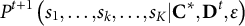
2.4 Sampling probability array
The sampling probability array also has the same dimensions as the decision array and contains the sampling probabilities of all dynamic eligible items at the current stage of form construction. The sampling probability of an item depends on the relative frequency of this item selected in the previous generation, the dynamic eligible array, and an error term. In particular, denote ${\mathbf{D}}^t=\sum \nolimits_{h=1}^H{\mathbf{D}}^{ht}$
, where
${\mathbf{D}}^t=\sum \nolimits_{h=1}^H{\mathbf{D}}^{ht}$
, where ${\mathbf{D}}^{ht}$
is the decision array for sample
${\mathbf{D}}^{ht}$
is the decision array for sample $h$
(
$h$
( $h=1,\dots, H$
) in generation
$h=1,\dots, H$
) in generation $t$
,
$t$
, $H$
is the user-defined population size, and
$H$
is the user-defined population size, and ${\mathbf{D}}^t$
is the frequency array for all items appearing in generation
${\mathbf{D}}^t$
is the frequency array for all items appearing in generation $t$
. Then, the sampling probability for an item
$t$
. Then, the sampling probability for an item ${s}_1,\dots, {s}_k,\dots, {s}_K$
in generation
${s}_1,\dots, {s}_k,\dots, {s}_K$
in generation $t+1$
is defined as
$t+1$
is defined as
 $$\begin{align}{P}^{t+1}\left({s}_1,\dots, {s}_k,\dots, {s}_K|{\mathbf{C}}^{\ast },{\mathbf{D}}^t,\varepsilon \right)=\frac{c_{s_1,\dots, {s}_k,\dots, {s}_K}^{\ast}\left({d}_{s_1,\dots, {s}_k,\dots, {s}_K}^t+\varepsilon \right)}{\sum \limits_{s_1^{\ast }=1}^S\cdots \sum \limits_{s_k^{\ast }={s}_{k-1}^{\ast }+1}^S\cdots \sum \limits_{s_K^{\ast }={s}_{K-1}^{\ast }+1}^S{c}_{s_1^{\ast },\dots, {s}_k^{\ast },\dots, {s}_K^{\ast}}^{\ast}\left({d}_{s_1^{\ast },\dots, {s}_k^{\ast },\dots, {s}_K^{\ast}}^t+\varepsilon \right)},\end{align}$$
where $\varepsilon$
is the error term representing a mutation factor. The mutation factor is proportional to the expected frequency of an eligible item in a generation, which, in turn, depends on the total number of fixed eligible items in the item pool. In particular,
$\varepsilon$
is the error term representing a mutation factor. The mutation factor is proportional to the expected frequency of an eligible item in a generation, which, in turn, depends on the total number of fixed eligible items in the item pool. In particular,
 $$\begin{align}\varepsilon ={B}_{ratio}H/\sum \limits_{s_1=1}^S\cdots \sum \limits_{s_k={s}_{k-1}+1}^S\cdots \sum \limits_{s_K={s}_{K-1}+1}^S{c}_{s_1,\dots, {s}_k,\dots, {s}_K},\end{align}$$
where ${B}_{ratio}$
is the bias ratio, a user-defined uniformizing positive constant controlling the diffusion of the probability distribution. When
${B}_{ratio}$
is the bias ratio, a user-defined uniformizing positive constant controlling the diffusion of the probability distribution. When ${B}_{ratio}$
closes to 0, the probability of an item mainly depends on this item’s frequency in the previous generation. The name of this algorithm, array histogram-based sampling, comes from this probability function. As
${B}_{ratio}$
closes to 0, the probability of an item mainly depends on this item’s frequency in the previous generation. The name of this algorithm, array histogram-based sampling, comes from this probability function. As ${B}_{ratio}$
tends to be positively infinite, the probability leans toward a uniform distribution. A larger
${B}_{ratio}$
tends to be positively infinite, the probability leans toward a uniform distribution. A larger ${B}_{ratio}$
leads to greater population heterogeneity, helping avoid local optima but increasing convergence time.
${B}_{ratio}$
leads to greater population heterogeneity, helping avoid local optima but increasing convergence time.
Note that the probability function used here Equations 1 and 2 is similar to that in the original NHBSA (Tsutsui, Reference Tsutsui2006, Equations 6–8) but differs from the one used in Kreitchmann et al. (Reference Kreitchmann, Abad and Sorrel2022, Equations 16 and 17). Kreitchmann et al. first randomly select a statement set, ${s}_1,\dots, {s}_k,\dots, {s}_{K-1}$
with
${s}_1,\dots, {s}_k,\dots, {s}_{K-1}$
with ${\mathbf{c}}_{s_1,\dots, {s}_k,\dots, {s}_{K-1}}^{\ast}\ne \mathbf{0}$
, where
${\mathbf{c}}_{s_1,\dots, {s}_k,\dots, {s}_{K-1}}^{\ast}\ne \mathbf{0}$
, where ${\mathbf{c}}_{s_1,\dots, {s}_k,\dots, {s}_{K-1}}^{\ast }$
is a vector in
${\mathbf{c}}_{s_1,\dots, {s}_k,\dots, {s}_{K-1}}^{\ast }$
is a vector in ${\mathbf{C}}^{\ast }$
, and then select an item from
${\mathbf{C}}^{\ast }$
, and then select an item from ${\mathbf{c}}_{s_1,\dots, {s}_k,\dots, {s}_{K-1}}^{\ast }$
based on the probability
${\mathbf{c}}_{s_1,\dots, {s}_k,\dots, {s}_{K-1}}^{\ast }$
based on the probability ${P}^{t+1}\left({s}_1,\dots, {s}_k,\dots, {s}_{K-1},{s}_K\right)$
, which depends on the relative frequency of
${P}^{t+1}\left({s}_1,\dots, {s}_k,\dots, {s}_{K-1},{s}_K\right)$
, which depends on the relative frequency of ${d}_{s_1,\dots, {s}_k,\dots, {s}_{K-1},{s}_K}^t$
in
${d}_{s_1,\dots, {s}_k,\dots, {s}_{K-1},{s}_K}^t$
in ${\mathbf{d}}_{s_1,\dots, {s}_k,\dots, {s}_{K-1}}^t$
, a vector in
${\mathbf{d}}_{s_1,\dots, {s}_k,\dots, {s}_{K-1}}^t$
, a vector in ${\mathbf{D}}^t$
. Accordingly, the error term for
${\mathbf{D}}^t$
. Accordingly, the error term for ${d}_{s_1,\dots, {s}_k,\dots, {s}_{K-1},{s}_K}^{t+1}$
is proportional to the expected frequency of the statement set,
${d}_{s_1,\dots, {s}_k,\dots, {s}_{K-1},{s}_K}^{t+1}$
is proportional to the expected frequency of the statement set, ${s}_1,\dots, {s}_k,\dots, {s}_{K-1}$
, in a generation. As a concrete example for triplets, Kreitchmann et al. first randomly select a set of eligible triplets containing the first two statements as, for example, Statements 1 and 2 (e.g., this set may contain three eligible triplets, {1,2,3}, {1,2,4}, and {1,2,5}), from all sets of eligible triples with the possible combinations of the first two statements (e.g., the sets of eligible triplets with the first two statements as {2,3}, {2,5}, {3,4}, etc.). Then, from the set of eligible triplets containing the first two statements as Statements 1 and 2, select a triplet (e.g., {1,2,3}) based on the sampling probabilities. In contrast, our AHBSA selects a triplet from the dynamic eligible array directly based on the sampling probabilities. Kreitchmann et al.’s first random selection of a subset of statements,
${s}_1,\dots, {s}_k,\dots, {s}_{K-1}$
, in a generation. As a concrete example for triplets, Kreitchmann et al. first randomly select a set of eligible triplets containing the first two statements as, for example, Statements 1 and 2 (e.g., this set may contain three eligible triplets, {1,2,3}, {1,2,4}, and {1,2,5}), from all sets of eligible triples with the possible combinations of the first two statements (e.g., the sets of eligible triplets with the first two statements as {2,3}, {2,5}, {3,4}, etc.). Then, from the set of eligible triplets containing the first two statements as Statements 1 and 2, select a triplet (e.g., {1,2,3}) based on the sampling probabilities. In contrast, our AHBSA selects a triplet from the dynamic eligible array directly based on the sampling probabilities. Kreitchmann et al.’s first random selection of a subset of statements, ${s}_1,\dots, {s}_k,\dots, {s}_{K-1}$
, adds randomness to the sampling process, leading to extremely slow convergence and a long running time. For example, the algorithm converged in 52 generations within 181 seconds with the new probability function for the real pair form we assembled later in the article. In contrast, with Kreitchmann et al.’s probability function, the algorithm did not converge in 2,000 iterations after 24 hours, and the mean objective function value at iteration 2,000 was still smaller than that at iteration 50 with the new probability function.
${s}_1,\dots, {s}_k,\dots, {s}_{K-1}$
, adds randomness to the sampling process, leading to extremely slow convergence and a long running time. For example, the algorithm converged in 52 generations within 181 seconds with the new probability function for the real pair form we assembled later in the article. In contrast, with Kreitchmann et al.’s probability function, the algorithm did not converge in 2,000 iterations after 24 hours, and the mean objective function value at iteration 2,000 was still smaller than that at iteration 50 with the new probability function.
2.5 Sampling process of assembling one form
For a form in the initial generation, each item is randomly selected from the eligible items in the current ${\mathbf{C}}^{\ast }$
. After each item selection,
${\mathbf{C}}^{\ast }$
. After each item selection, ${\mathbf{C}}^{\ast }$
is updated to conform to between-item constraints. See Algorithm 1 for the schematic description of the sampling process of assembling an initial form. The sampling process for selecting a candidate form
${\mathbf{C}}^{\ast }$
is updated to conform to between-item constraints. See Algorithm 1 for the schematic description of the sampling process of assembling an initial form. The sampling process for selecting a candidate form $h$
in the subsequent generation
$h$
in the subsequent generation $t+1$
involves two steps. First, generate two random thresholds,
$t+1$
involves two steps. First, generate two random thresholds, ${m}_1$
and
${m}_1$
and ${m}_2$
, copy
${m}_2$
, copy ${d}_{s_1,\dots, {s}_k,\dots, {s}_K}^{ht}$
with
${d}_{s_1,\dots, {s}_k,\dots, {s}_K}^{ht}$
with ${m}_1\le {s}_k\le {m}_2$
to
${m}_1\le {s}_k\le {m}_2$
to ${\mathbf{D}}^{\ast }$
, the candidate decision array, and update
${\mathbf{D}}^{\ast }$
, the candidate decision array, and update ${\mathbf{C}}^{\ast }$
. Second, for every unselected item in the form, select it from the eligible items in the current
${\mathbf{C}}^{\ast }$
. Second, for every unselected item in the form, select it from the eligible items in the current ${\mathbf{C}}^{\ast }$
based on the probability
${\mathbf{C}}^{\ast }$
based on the probability ${P}^{t+1}\left({s}_1,\dots, {s}_k,\dots, {s}_K|{\mathbf{C}}^{\ast },{\mathbf{D}}^t,\varepsilon \right)$
. The first step involves copying the template, representing the crossover operator, and the second step involves probabilistic sampling, representing the mutation operator (Kreitchmann et al., Reference Kreitchmann, Abad and Sorrel2022; Tsutsui, Reference Tsutsui2006). Algorithm 2 provides a schematic description of selecting a candidate form in a subsequent generation. A candidate form is not necessarily a final form in generation
${P}^{t+1}\left({s}_1,\dots, {s}_k,\dots, {s}_K|{\mathbf{C}}^{\ast },{\mathbf{D}}^t,\varepsilon \right)$
. The first step involves copying the template, representing the crossover operator, and the second step involves probabilistic sampling, representing the mutation operator (Kreitchmann et al., Reference Kreitchmann, Abad and Sorrel2022; Tsutsui, Reference Tsutsui2006). Algorithm 2 provides a schematic description of selecting a candidate form in a subsequent generation. A candidate form is not necessarily a final form in generation $t+1$
. Rather, all
$t+1$
. Rather, all $H$
candidate forms in generation
$H$
candidate forms in generation $t+1$
and the final
$t+1$
and the final $H$
forms in generation
$H$
forms in generation $t$
are combined, and the first
$t$
are combined, and the first $H$
forms having the largest objective function values are selected as the final forms in generation
$H$
forms having the largest objective function values are selected as the final forms in generation $t+1$
, which is the selection operator.
$t+1$
, which is the selection operator.
Schematic description of sampling process of one form in the initial generation.

Schematic description of sampling process of one form in a noninitial generation.

2.6 Whole loop
The entire AHBSA iteration process is described schematically in Algorithm 3. Users first create a fixed eligible item array, $\mathbf{C}$
, based on within-item constraints, a function updating the dynamic eligible item array,
$\mathbf{C}$
, based on within-item constraints, a function updating the dynamic eligible item array, ${\mathbf{C}}^{\ast }$
, based on between-item constraints, and a function to calculate the objective function values. Users also need to define the population size (
${\mathbf{C}}^{\ast }$
, based on between-item constraints, and a function to calculate the objective function values. Users also need to define the population size ( $H$
) in each generation, the number of items in each form (
$H$
) in each generation, the number of items in each form ( $I$
), the bias ratio (
$I$
), the bias ratio ( ${B}_{ratio}$
), and the convergence criterion (e.g., all decision arrays in a generation are the same; the maximum number of generations or time is reached; and the variance of the maximum within-generation objective function values across certain consecutive generations is smaller than a threshold). A larger population size enables the algorithm to explore a broader search space, allowing it to find better solutions, but it also slows convergence. The AHBSA iteration begins with the initial generation and proceeds to subsequent generations until the convergence criterion is met.
${B}_{ratio}$
), and the convergence criterion (e.g., all decision arrays in a generation are the same; the maximum number of generations or time is reached; and the variance of the maximum within-generation objective function values across certain consecutive generations is smaller than a threshold). A larger population size enables the algorithm to explore a broader search space, allowing it to find better solutions, but it also slows convergence. The AHBSA iteration begins with the initial generation and proceeds to subsequent generations until the convergence criterion is met.
Schematic description of the whole loop of AHBSA.

3 Real test assemblies
We first applied AHBSA to a real item pool to assemble three real test forms: a Likert form, an MFCQ with pairs, and an MFCQ with triplets. We also assembled these forms using MIP and generated random forms that conform to the constraints without an objective function. We compared the performance of the three algorithms in terms of the expected reliabilities and assembly times of the assembled forms.
3.1 Real statement pool
The statement pool comprised 91 statements from the student questionnaire in the Organization for Economic Co-operation and Development (OECD) Survey on Social and Emotional Skills 2019 (SSES; OECD, 2021). Among the 91 statements, there were 24 negative statements. The 91 statements were selected from the 120 statements in SSES, with 29 statements removed by OECD (2021) from the student or parent questionnaire based on scaling analysis outcomes and item content (OECD, 2021, Table 12.12). The questionnaire measured five domains (collaboration, task performance, engaging with others, emotional regulation, and open-mindedness), each containing three skills (e.g., the collaboration domain included co-operation, empathy, and trust; a total of 15 skills). Each statement measured only one domain and only one skill. Each domain was assessed using 17–19 statements from a total of 91.
Because the objective functions were related to Fisher information, we needed the parameters of these statements based on an IRT model. We chose the two-parameter logistic model (2PLM; Birnbaum, Reference Birnbaum, Lord and Novick1968), where the probability of answering item $i$
correctly (i.e., agreeing with a statement) conditional on a latent score of trait
$i$
correctly (i.e., agreeing with a statement) conditional on a latent score of trait ${v}_i$
(
${v}_i$
( ${\theta}_{v_i}$
) that item
${\theta}_{v_i}$
) that item $i$
measures:
$i$
measures:
 $$\begin{align}P\left({x}_i=1|{\theta}_{v_i}\right)={\left[1+\exp \left(-{a}_i{\theta}_{v_i}-{b}_i\right)\right]}^{-1},\end{align}$$
 $$\begin{align}P\left({x}_i=0|{\theta}_{v_i}\right)=1-P\left({x}_i=1|{\theta}_{v_i}\right),\end{align}$$
where ${x}_i$
is the coded item response (1=agree, and 0=disagree);
${x}_i$
is the coded item response (1=agree, and 0=disagree); ${a}_i$
and
${a}_i$
and ${b}_i$
are item
${b}_i$
are item $i$
’s slope (discrimination) and intercept parameters, respectively;
$i$
’s slope (discrimination) and intercept parameters, respectively; $-{b}_i/{a}_i$
is referred to as item
$-{b}_i/{a}_i$
is referred to as item $i$
’s difficulty parameter. The same calibration sample used in the SSES report (OECD, 2021) was used to calibrate the 2PLM parameters for the 91 statements.Footnote
2
The actual Likert data had five response categories, with scores ranging from 0 to 4, corresponding to strongly disagree to strongly agree. The real data were dichotomized (scores 3 and 4 were recoded as 1, and others as 0) for the 2PLM calibration, and negative statements were scored in reverse. We set up a similar IRT calibration to that in OECD (2021): a multigroup 2PLM with the cohort ID (younger and old) as the grouping variable and the senate weightsFootnote
3
for test takers.Footnote
4
The exception was that OECD used the generalized partial credit model (GPCM), while we used the 2PLM. The 2PLM calibrations were conducted separately by the five domains, and the discrimination and difficulty parameters for each statement were estimated. For negative statements, their parameters were transformed back to match the negative direction. Then, each domain’s maximum a posteriori (MAP) scores were estimated, and the weighted (by senate weights) correlation matrix for the five domains was calculated (Table 1).
$i$
’s difficulty parameter. The same calibration sample used in the SSES report (OECD, 2021) was used to calibrate the 2PLM parameters for the 91 statements.Footnote
2
The actual Likert data had five response categories, with scores ranging from 0 to 4, corresponding to strongly disagree to strongly agree. The real data were dichotomized (scores 3 and 4 were recoded as 1, and others as 0) for the 2PLM calibration, and negative statements were scored in reverse. We set up a similar IRT calibration to that in OECD (2021): a multigroup 2PLM with the cohort ID (younger and old) as the grouping variable and the senate weightsFootnote
3
for test takers.Footnote
4
The exception was that OECD used the generalized partial credit model (GPCM), while we used the 2PLM. The 2PLM calibrations were conducted separately by the five domains, and the discrimination and difficulty parameters for each statement were estimated. For negative statements, their parameters were transformed back to match the negative direction. Then, each domain’s maximum a posteriori (MAP) scores were estimated, and the weighted (by senate weights) correlation matrix for the five domains was calculated (Table 1).
Correlation matrix of five domains

Note: D1, collaboration; D2, task performance; D3, engaging with others; D4, emotional regulation; D5, open-mindedness.
3.2 Form constraints
The constraints for different forms were slightly different, as described below.
3.2.1 Likert form
In the Likert form, a statement is an item; thus, there was no within-item constraint. There were two between-item constraints. The first one was that a statement appeared at most once in the form, which can be denoted as
 $$\begin{align}\sum \limits_{i=1}^I\mathrm{I}\left(s\in {\mathbf{g}}_i\right)\le 1,\ \mathrm{for}\;s=1,\dots, S,\end{align}$$
where $I$
is the number of items in a test,
$I$
is the number of items in a test, ${\mathbf{g}}_i$
is the set of statement ID(s) used in item
${\mathbf{g}}_i$
is the set of statement ID(s) used in item $i$
(containing 1, 2, and 3 statements for a Likert, pair, and triplet item, respectively), and
$i$
(containing 1, 2, and 3 statements for a Likert, pair, and triplet item, respectively), and $\mathrm{I}\left(s\in {\mathbf{g}}_i\right)$
is an indicator function. The second one was that each skill appeared exactly four times in the form,
$\mathrm{I}\left(s\in {\mathbf{g}}_i\right)$
is an indicator function. The second one was that each skill appeared exactly four times in the form,
 $$\begin{align}\sum \limits_{i=1}^I\mathrm{I}\left(r\in {\mathbf{r}}_i\right)=4,\ \mathrm{for}\;r=1,\dots, R,\end{align}$$
where $r$
refers to a skill,
$r$
refers to a skill, $R$
is the total number of skills measured by the statement pool,
$R$
is the total number of skills measured by the statement pool, ${\mathbf{r}}_i$
is the set of skill(s) measured by item
${\mathbf{r}}_i$
is the set of skill(s) measured by item $i$
. The second constraint implied a form length of 60 items.
$i$
. The second constraint implied a form length of 60 items.
3.2.2 Pair form
There was one within-item constraint: the two statements in a pair measured two different domains, that is,
 $$\begin{align}{v}_{is_k}\ne {v}_{is_{k^{\ast }}},\ \mathrm{for}\;k\ne {k}^{\ast}\;\mathrm{and}\;i=1,\dots, I,\end{align}$$
where ${v}_{is_k}$
and
${v}_{is_k}$
and ${v}_{is_{k^{\ast }}}$
refer to the two domains measured by the
${v}_{is_{k^{\ast }}}$
refer to the two domains measured by the $k$
th and
$k$
th and ${k}^{\ast }$
th statements, respectively, in an item
${k}^{\ast }$
th statements, respectively, in an item $i$
. There were two between-item constraints. The first one was the same as the first one in the Likert form (a statement appeared only once in a form, Equation 5). The second one was that a skill was paired with a domain only once:
$i$
. There were two between-item constraints. The first one was the same as the first one in the Likert form (a statement appeared only once in a form, Equation 5). The second one was that a skill was paired with a domain only once:
 $$\begin{align}\sum \limits_{i=1}^I\mathrm{I}\left(r\in {\mathbf{r}}_i\wedge r\notin {\mathbf{r}}_v\wedge v\in {\mathbf{v}}_i\right)=1,\ \mathrm{for}\;r=1,\dots, R,\mathrm{and}\;v=1,\dots, V,\end{align}$$
where ${\mathbf{r}}_v$
refers to the set of skills under domain
${\mathbf{r}}_v$
refers to the set of skills under domain $v$
,
$v$
, ${\mathbf{v}}_i$
denotes the set of domains measured by item
${\mathbf{v}}_i$
denotes the set of domains measured by item $i$
, and
$i$
, and $V$
is the total number of domains. This constraint also implied that each combination of two domains in a pair appeared three times, resulting in a total of 30 pairs.
$V$
is the total number of domains. This constraint also implied that each combination of two domains in a pair appeared three times, resulting in a total of 30 pairs.
3.2.3 Triplet form
There was only one within-item constraint similar to that on the pair form: each statement in a triplet measured a different domain Equation 7. There were three between-item constraints. The first one was the same as the first one in the other two forms Equation 5. The second one was that each combination of three domains in a triplet appeared only twice in the form, implying a form length of 20 triplets:
 $$\begin{align}\sum \limits_{i=1}^I\mathrm{I}\left({\mathbf{v}}_i={\mathbf{v}}_l\right)=2,\ \mathrm{for}\ \forall {\mathbf{v}}_l\in {C}_3^{\mathbf{V}},\end{align}$$
where ${\mathbf{v}}_l$
is a unique combination
${\mathbf{v}}_l$
is a unique combination $l$
of three domains. The third one was that a skill appeared at most once in each combination of three domains:
$l$
of three domains. The third one was that a skill appeared at most once in each combination of three domains:
 $$\begin{align}\sum \limits_{i=1}^I\mathrm{I}\left({\mathbf{v}}_i={\mathbf{v}}_l\wedge r\in {\mathbf{r}}_{{\mathbf{v}}_l}\right)\le 1,\ \mathrm{for}\ \forall {\mathbf{v}}_l\in {C}_3^{\mathbf{V}}\;\mathrm{and}\;r=1,\dots, R,\end{align}$$
where ${\mathbf{r}}_{{\mathbf{v}}_l}$
is the set of skills in combination
${\mathbf{r}}_{{\mathbf{v}}_l}$
is the set of skills in combination $l$
of three domains.
$l$
of three domains.
Constraints on statement direction (i.e., positively versus negatively worded and keyed statements) were not considered in the real forms because the number of negative statements in the pool was inadequate. However, constraints on statement direction were considered in the later simulation study. Using negatively keyed statements in personality assessment is a long-standing practice designed to increase attentiveness and decrease acquiescence responding (Cronbach, Reference Cronbach1950), although its advisability and treatment remain a research topic (Lee et al., Reference Lee, Joo, Zhou and Son2022).
3.3 Objective functions
The objective functions differed by the forms and ATA methods. For MIP, the objective function was to maximize the weighted average of the traces of the FTI matrices across quadrature points (i.e., T-optimality). The weights were the normalized densities of the quadrature points based on a multivariate standard normal distribution with the interdomain correlation matrix estimated above, that is,
 $$\begin{align}\operatorname{Max}\sum \limits_{w=1}^W\mathrm{trace}\left(F\left({\boldsymbol{\unicode{x3b8}}}_w\right)\right)\phi \left({\boldsymbol{\unicode{x3b8}}}_w|{\boldsymbol{\Sigma}}_{\boldsymbol{\unicode{x3b8}}}\right)/\sum \limits_{w=1}^W\phi \left({\boldsymbol{\unicode{x3b8}}}_w|{\boldsymbol{\Sigma}}_{\boldsymbol{\unicode{x3b8}}}\right),\end{align}$$
where ${\boldsymbol{\unicode{x3b8}}}_w$
is a quadrature vector
${\boldsymbol{\unicode{x3b8}}}_w$
is a quadrature vector $w$
,
$w$
, $W$
is the total number of quadrature vectors,
$W$
is the total number of quadrature vectors, $F\left({\boldsymbol{\unicode{x3b8}}}_w\right)$
is the FTI of
$F\left({\boldsymbol{\unicode{x3b8}}}_w\right)$
is the FTI of ${\boldsymbol{\unicode{x3b8}}}_w$
, and
${\boldsymbol{\unicode{x3b8}}}_w$
, and $\phi \left({\boldsymbol{\unicode{x3b8}}}_w|{\boldsymbol{\Sigma}}_{\boldsymbol{\unicode{x3b8}}}\right)$
is the density of
$\phi \left({\boldsymbol{\unicode{x3b8}}}_w|{\boldsymbol{\Sigma}}_{\boldsymbol{\unicode{x3b8}}}\right)$
is the density of ${\boldsymbol{\unicode{x3b8}}}_w$
based on the multivariate standard normal distribution with the interdomain correlation matrix
${\boldsymbol{\unicode{x3b8}}}_w$
based on the multivariate standard normal distribution with the interdomain correlation matrix ${\boldsymbol{\Sigma}}_{\boldsymbol{\unicode{x3b8}}}$
(Table 1). For quadrature vectors, we used three quadrature points (−1, 0, 1) on each domain. Thus, the total number of quadrature vectors (
${\boldsymbol{\Sigma}}_{\boldsymbol{\unicode{x3b8}}}$
(Table 1). For quadrature vectors, we used three quadrature points (−1, 0, 1) on each domain. Thus, the total number of quadrature vectors ( $W$
) was 125 (
$W$
) was 125 ( ${5}^3$
).
${5}^3$
).
Test information $F\left(\boldsymbol{\unicode{x3b8}} \right)$
is the sum of all item information
$F\left(\boldsymbol{\unicode{x3b8}} \right)$
is the sum of all item information ${f}_i\left(\boldsymbol{\unicode{x3b8}} \right)$
in a test:
${f}_i\left(\boldsymbol{\unicode{x3b8}} \right)$
in a test:
 $$\begin{align}F\left(\boldsymbol{\unicode{x3b8}} \right)=\sum \limits_{i=1}^I{f}_i\left(\boldsymbol{\unicode{x3b8}} \right),\end{align}$$
where $I$
is the number of items in a test. The general formula for the Fisher item information of item
$I$
is the number of items in a test. The general formula for the Fisher item information of item $i$
(Fu, Tan, et al., Reference Fu, Tan and Kyllonen2024, Equation 16) is
$i$
(Fu, Tan, et al., Reference Fu, Tan and Kyllonen2024, Equation 16) is
 $$\begin{align}{f}_i\left(\boldsymbol{\unicode{x3b8}} \right)=\sum \limits_{z=0}^{Z_i}\frac{\partial G\left({x}_i=z|\boldsymbol{\unicode{x3b8}} \right)}{\partial \boldsymbol{\unicode{x3b8}}}{\left[\frac{\partial G\left({x}_i=z|\boldsymbol{\unicode{x3b8}} \right)}{\partial \boldsymbol{\unicode{x3b8}}}\right]}^{\prime }{\left[G\left({x}_i=z|\boldsymbol{\unicode{x3b8}} \right)\right]}^{-1},\end{align}$$
where $G\left({x}_i=z|\boldsymbol{\unicode{x3b8}} \right)$
is the item response function based on an IRT model, and
$G\left({x}_i=z|\boldsymbol{\unicode{x3b8}} \right)$
is the item response function based on an IRT model, and $z$
is the coded item response (i.e., an integer from 0 to
$z$
is the coded item response (i.e., an integer from 0 to ${Z}_i$
, where
${Z}_i$
, where ${Z}_i$
is the maximum possible score of item
${Z}_i$
is the maximum possible score of item $i$
). In
$i$
). In ${f}_i\left(\boldsymbol{\unicode{x3b8}} \right)$
, an entry is 0 if either of its row and column traits is not measured by item
${f}_i\left(\boldsymbol{\unicode{x3b8}} \right)$
, an entry is 0 if either of its row and column traits is not measured by item $i$
.
$i$
.
For the Likert form, each item included one statement, and each statement measured only one domain. Thus, in ${f}_i\left(\boldsymbol{\unicode{x3b8}} \right)$
, all but the diagonal value for the domain measured by item
${f}_i\left(\boldsymbol{\unicode{x3b8}} \right)$
, all but the diagonal value for the domain measured by item $i$
are 0s. The item information for the Likert scale was estimated using the 2PLM Equations 3 and 4. For the 2PLM, the item information function of item
$i$
are 0s. The item information for the Likert scale was estimated using the 2PLM Equations 3 and 4. For the 2PLM, the item information function of item $i$
on a latent score of domain
$i$
on a latent score of domain ${v}_i$
(
${v}_i$
( ${\theta}_{v_i}$
) is (Muraki, Reference Muraki1993, Equation 12)
${\theta}_{v_i}$
) is (Muraki, Reference Muraki1993, Equation 12)
 $$\begin{align}{f}_i{\left(\boldsymbol{\unicode{x3b8}} \right)}_{v_i{v}_i}={a}_i^2P\left({x}_i=1|{\theta}_{v_i}\right)P\left({x}_i=0|{\theta}_{v_i}\right).\end{align}$$
For the pair form, item information was estimated using the multi-unidimensional pairwise preference with the 2PLM (MUPP-2PLM; Morillo et al., Reference Morillo, Leenen, Abad, Hontangas, de la Torre and Ponsoda2016). We code the selection of the first statement as response score 1 and the selection of the second statement as 0 (i.e., ${x}_i$
= 0, 1). Then, the item response function of the MUPP-2PLM is
${x}_i$
= 0, 1). Then, the item response function of the MUPP-2PLM is
 $$\begin{align}{P}^{\ast}\left({x}_i=1|\boldsymbol{\unicode{x3b8}} \right)={\left[1+\exp \left({a}_{i2}{\theta}_{v_{i2}}+{b}_{i2}-{a}_{i1}{\theta}_{v_{i1}}-{b}_{i1}\right)\right]}^{-1}={\left[1+\exp \left({a}_{i2}{\theta}_{v_{i2}}-{a}_{i1}{\theta}_{v_{i1}}-{b}_{i12}\right)\right]}^{-1},\end{align}$$
 $$\begin{align}{P}^{\ast}\left({x}_i=0|\boldsymbol{\unicode{x3b8}} \right)=1-{P}^{\ast}\left({x}_i=1|\boldsymbol{\unicode{x3b8}} \right),\end{align}$$
where ${\theta}_{v_{i1}}$
and
${\theta}_{v_{i1}}$
and ${\theta}_{v_{i2}}$
are two latent scores on the two traits measured by Statements 1 and 2 in pair item
${\theta}_{v_{i2}}$
are two latent scores on the two traits measured by Statements 1 and 2 in pair item $i$
, respectively;
$i$
, respectively; ${a}_{i1}$
and
${a}_{i1}$
and ${a}_{i2}$
are the slope parameters of Statements 1 and 2, respectively;
${a}_{i2}$
are the slope parameters of Statements 1 and 2, respectively; ${b}_{i1}$
and
${b}_{i1}$
and ${b}_{i2}$
are the intercepts; and
${b}_{i2}$
are the intercepts; and ${b}_{i12}={b}_{i1}-{b}_{i2}$
is the estimable intercept, as only one of the two intercepts is identified in Equation 15. Then, the item information matrix based on MUPP-2PLM (Kreitchmann et al., Reference Kreitchmann, Abad and Sorrel2022, Equation 10) is
${b}_{i12}={b}_{i1}-{b}_{i2}$
is the estimable intercept, as only one of the two intercepts is identified in Equation 15. Then, the item information matrix based on MUPP-2PLM (Kreitchmann et al., Reference Kreitchmann, Abad and Sorrel2022, Equation 10) is
 $$\begin{align}{f}_i{\left(\boldsymbol{\unicode{x3b8}} \right)}_{{\mathbf{v}}_i{\mathbf{v}}_i}=\left[\begin{array}{cc}{a}_{i1}^2{P}^{\ast}\left({x}_i=1|\boldsymbol{\unicode{x3b8}} \right){P}^{\ast}\left({x}_i=0|\boldsymbol{\unicode{x3b8}} \right)& -{a}_{i1}{a}_{i2}{P}^{\ast}\left({x}_i=1|\boldsymbol{\unicode{x3b8}} \right){P}^{\ast}\left({x}_i=0|\boldsymbol{\unicode{x3b8}} \right)\\ {}-{a}_{i1}{a}_{i2}{P}^{\ast}\left({x}_i=1|\boldsymbol{\unicode{x3b8}} \right){P}^{\ast}\left({x}_i=0|\boldsymbol{\unicode{x3b8}} \right)& {a}_{i2}^2{P}^{\ast}\left({x}_i=1|\boldsymbol{\unicode{x3b8}} \right){P}^{\ast}\left({x}_i=0|\boldsymbol{\unicode{x3b8}} \right)\end{array}\right],\end{align}$$
where ${\mathbf{V}}_i$
is the set of two domains measured by pair item
${\mathbf{V}}_i$
is the set of two domains measured by pair item $i$
, and
$i$
, and ${f}_i{\left(\boldsymbol{\unicode{x3b8}} \right)}_{{\mathbf{v}}_i{\mathbf{v}}_i}$
refers to the subset of the item information matrix related to the two domains measured by item
${f}_i{\left(\boldsymbol{\unicode{x3b8}} \right)}_{{\mathbf{v}}_i{\mathbf{v}}_i}$
refers to the subset of the item information matrix related to the two domains measured by item $i$
.
$i$
.
The triplet form’s IRT calibration model was the Triplet-2PLM (Fu, Reference Fu2025). A triple item has six possible ranking patterns, 123, 132, 213, 231, 312, and 321 (e.g., 123 represents that Statement 1 is ranked as the first, Statement 2 is ranked as the second, and Statement 3 is ranked as the last), and code them as response scores 0–5, respectively. The item response function of Triplet-2PLM for item score 0 (i.e., the ranking pattern 123):
 $$\begin{align}&{P}^{\#}\left({x}_i=0|\boldsymbol{\unicode{x3b8}} \right)=\nonumber\\ &\quad{}{\left[1+\exp \left({a}_{i2}{\theta}_{v_{i2}}+{b}_{i2}-{a}_{i1}{\theta}_{v_{i1}}-{b}_{i1}\right)+\exp \left({a}_{i3}{\theta}_{i3}+{b}_{i3}-{a}_{i1}{\theta}_{v_{i1}}-{b}_{i1}\right)\right]}^{-1}\nonumber\\&\quad{}{\left[1+\exp \left({a}_{i3}{\theta}_{i3}+{b}_{i3}-{a}_{i2}{\theta}_{v_{i2}}-{b}_{i2}\right)\right]}^{-1}.\end{align}$$
The item response functions for other item scores are analogous to Equation 18. Note that for ${b}_{i1}$
,
${b}_{i1}$
, ${b}_{i2}$
, and
${b}_{i2}$
, and ${b}_{i3}$
, only two of them can be identified in Equation 18. We can fix one of the
${b}_{i3}$
, only two of them can be identified in Equation 18. We can fix one of the $b$
values to identify the model. In the MUPP-2PLM and Triplet-2PLM, each statement’s slope and intercept parameters correspond to those in the 2PLM. In the current test assembly, the parameters of each statement were assumed to be known and provided by their 2PLM calibration. To calculate the Fisher item information, we need to derive the first derivative of Equation 18 with respect to each domain measured by triplet item
$b$
values to identify the model. In the MUPP-2PLM and Triplet-2PLM, each statement’s slope and intercept parameters correspond to those in the 2PLM. In the current test assembly, the parameters of each statement were assumed to be known and provided by their 2PLM calibration. To calculate the Fisher item information, we need to derive the first derivative of Equation 18 with respect to each domain measured by triplet item $i$
. To avoid tedious derivations, we can use the R package Deriv (Clausen & Sokol, Reference Clausen and Sokol2020) to obtain the symbolic derivatives of Equation 18 (Fu, Tan, et al., Reference Fu, Tan and Kyllonen2024).Footnote
5
Then, we can use Equation 13 to compute the subset of the item information matrix
$i$
. To avoid tedious derivations, we can use the R package Deriv (Clausen & Sokol, Reference Clausen and Sokol2020) to obtain the symbolic derivatives of Equation 18 (Fu, Tan, et al., Reference Fu, Tan and Kyllonen2024).Footnote
5
Then, we can use Equation 13 to compute the subset of the item information matrix ${f}_i{\left(\boldsymbol{\unicode{x3b8}} \right)}_{{\mathbf{v}}_i{\mathbf{v}}_i}$
related to the three domains measured by a triplet item.
${f}_i{\left(\boldsymbol{\unicode{x3b8}} \right)}_{{\mathbf{v}}_i{\mathbf{v}}_i}$
related to the three domains measured by a triplet item.
For AHBSA, the objective function was to maximize the average of the reliabilities of the five MAP latent domain score estimates on the quadrature vectors (i.e., A-optimality):
 $$\begin{align}\operatorname{Max}\sum \limits_{v=1}^V{\widehat{\rho}}_{{\widehat{\theta}}_v}^2/V,\end{align}$$
where $V$
(= 5) is the number of domains measured by a test, and
$V$
(= 5) is the number of domains measured by a test, and ${\widehat{\rho}}_{{\widehat{\theta}}_v}^2$
is the estimated reliability of a latent score estimate in domain
${\widehat{\rho}}_{{\widehat{\theta}}_v}^2$
is the estimated reliability of a latent score estimate in domain $v$
. The reliability of a domain was estimated based on the expected error variance of this domain’s MAP estimates, which, in turn, was the corresponding diagonal element in the expected inverse matrix of the test information plus the inverse interdomain correlation matrix across the quadrature vectors, where the normalized densities of the quadrature vectors were used as the weights in the expectation calculation. The computational formulas (Fu, Tan, et al., Reference Fu, Tan and Kyllonen2024, Equation 23; Kreitchmann et al., Reference Kreitchmann, Abad and Sorrel2022, Equation 18) are
$v$
. The reliability of a domain was estimated based on the expected error variance of this domain’s MAP estimates, which, in turn, was the corresponding diagonal element in the expected inverse matrix of the test information plus the inverse interdomain correlation matrix across the quadrature vectors, where the normalized densities of the quadrature vectors were used as the weights in the expectation calculation. The computational formulas (Fu, Tan, et al., Reference Fu, Tan and Kyllonen2024, Equation 23; Kreitchmann et al., Reference Kreitchmann, Abad and Sorrel2022, Equation 18) are
 $$\begin{align}{\widehat{e}}_{\theta_v\mid {\widehat{\theta}}_v}=\left[\sum \limits_{w=1}^W{\left[F\left({\boldsymbol{\unicode{x3b8}}}_w\right)+{\boldsymbol{\Sigma}}_{\boldsymbol{\unicode{x3b8}}}^{-1}\right]}^{-1}\phi \Big({\boldsymbol{\unicode{x3b8}}}_w|{\boldsymbol{\Sigma}}_{\boldsymbol{\unicode{x3b8}}}\left)/\sum \limits_{w=1}^W\phi \right({\boldsymbol{\unicode{x3b8}}}_w|{\boldsymbol{\Sigma}}_{\boldsymbol{\unicode{x3b8}}}\Big)\right],\end{align}$$
 $$\begin{align}{\widehat{\rho}}_{{\widehat{\theta}}_v}^2=\frac{\operatorname{var}\left({\theta}_v\right)-{\widehat{e}}_{\theta_v\mid {\widehat{\theta}}_v}}{\operatorname{var}\left({\theta}_v\right)}=1-{\widehat{e}}_{\theta_v\mid {\widehat{\theta}}_v},\end{align}$$
where ${\widehat{e}}_{\theta_v\mid {\widehat{\theta}}_v}$
is the expected error variance estimate of a latent score estimate in domain
${\widehat{e}}_{\theta_v\mid {\widehat{\theta}}_v}$
is the expected error variance estimate of a latent score estimate in domain $v$
. In Equation 21, the true value of the variance of
$v$
. In Equation 21, the true value of the variance of ${\theta}_v$
(i.e., 1) is applied, and we refer to it as theoretical reliability.
${\theta}_v$
(i.e., 1) is applied, and we refer to it as theoretical reliability.
3.4 Computer programs and setups
All analyses were conducted using the R 4.4.1 program (R Core Team, 2024). The weighted multigroup 2PLM calibrations were carried out using the mirt package (Chalmers, Reference Chalmers2012) with the default settings.
The MIP models were implemented in the eatATA package (Becker et al., Reference Becker, Debeer, Sachse and Weirich2021), and the GNU Linear Programming Kit (GLPK) solver (Makhorin, Reference Makhorin2018) was used. See Fu (Reference Fu2025) for discussions and demonstrations of assembling MFCQs using MIP. We wrote R codes for the two MFC forms to generate the eligible item pools from the statement pool before applying MIP to the item pools. The number of eligible items in the pair and triplet pools that met the within-item constraints was 3,311 and 60,209, respectively.
We developed an R program to implement the AHBSA described previously. The bias ratio ${B}_{ratio}$
was set to 2-4, as in Kreitchmann et al. (Reference Kreitchmann, Abad and Sorrel2022).Footnote
6
The population size was set to 50. The convergence criterion was that all 50 assembled forms in a generation were identical.
${B}_{ratio}$
was set to 2-4, as in Kreitchmann et al. (Reference Kreitchmann, Abad and Sorrel2022).Footnote
6
The population size was set to 50. The convergence criterion was that all 50 assembled forms in a generation were identical.
The random forms were generated by the initial step of the AHBSA (see Algorithm 1). For each form, 1,000 random replicate forms were generated.
The theoretical reliabilities of domain scores in the assembled forms were used to compare the performance of the three ATA methods. For the random forms, the theoretical reliabilities are the averages across the 1,000 replicates. We also compared the running times of different methods.
All runs in this article were conducted across multiple servers in a Linux grid. The sample codes used in the real study are provided on GitHub (https://github.com/liu6171/AHBSA).
3.5 Results
The comparisons of the five domains’ MAP theoretical reliabilities and running times among AHBSA, MIP, and random sampling are provided in Table 2. For the Likert form, the objective functions on test information and reliabilities are equivalent because each statement is unidimensional. The AHBSA and MIP achieved the same reliabilities, indicating that the AHBSA found the optimal solution for the Likert form. Their reliabilities were slightly higher than those of a random form by an average of 0.03.
Comparisons of theoretical reliabilities and running times on real forms

Note: Rel1–Rel5, reliabilities of Domains 1–5 score estimates; AHBSA, array histogram-based sampling algorithm; MIP, mixed integer programming.
aMean reliabilities over 1,000 random replicates.
For the pair form, AHBSA’s reliabilities were, on average, 0.08 higher than MIP’s, while MIP’s were close to a random form’s (with an average difference of 0.02). However, for the triplet form, the AHBSA had an average reliability of 0.01 higher than MIP, which, in turn, had an average reliability of 0.05 higher than that of a random form.
The triplet form had higher reliabilities than the Likert and pair forms across ATA algorithms, consistent with previous studies (e.g., Fu, Tan, et al., Reference Fu, Tan and Kyllonen2024; Joo et al., Reference Joo, Lee and Stark2018). However, the pair forms assembled by MIP and the random pair forms had lower reliabilities than the Likert forms assembled by the three methods, and the best pair form assembled by AHBSA had reliabilities similar to those of the best Likert form assembled by MIP and AHBSA. Note that statement direction has no impact on a Likert form’s reliability, while MFC items with mixed-direction statements will boost the reliability of an MFC form (Brown & Maydeu-Olivares, Reference Brown and Maydeu-Olivares2011; Bürkner, Reference Bürkner2022; Fu et al., Reference Fu, Tan and Kyllonen2025).
The AHBSA found the best solutions in all three forms. Especially for the pair form, the reliabilities AHBSA achieved were notably higher than those of MIP. However, the AHBSA runs were significantly longer than the MIP runs. Especially for the triplet form, the AHBSA run took more than 22 hours, while the MIP run converged in merely 7.7 seconds. The AHBSA’s slowness is related to the arrays used in the AHBSA, whose sizes grow exponentially with the number of statements in a pool, the item block size, and the number of quadrature points. We will discuss running times more later in the discussion section.
4 Simulation study
The purposes of the simulation study were two-fold. First, we wanted to verify the comparison results from the real data in a more general setting. Thus, the simulation study used the same construct and assembled the same forms as in the real example. Second, we wanted to check some factors that may impact test assemblies but could not be manipulated in the real data. In particular, we controlled four factors in the simulation study as detailed below: assembled form, ATA method, size of the statement pool, and item direction.
4.1 Study design
There were four controlled factors. The first two have been controlled in the real example: assembled form (Likert, pair, and triplet forms) and ATA method (AHBSA, MIP, and Random).
The third one was the size of the statement pool with three levels: 60, 90, and 120. We expected the form reliabilities and running time to increase with the statement pool size.
The fourth one was the item direction with three levels. The first level was that half of the statement pool was negative, and there was a constraint on item direction on the assembled form (referred to as Dir). The second level was the same as the first but had no constraint on item direction (referred to as NonDir). The third level was that the statement pool was all positive (referred to as Pos).
The simulation study assembled the three test forms that measured the same constructs (i.e., five domains, each with three skills) and had the same test length as the real example. The simulated statement pools had an even number of statements across domains and skills for the positive statement pools, and across statement directions for the mixed-direction statement pools. The discrimination parameters were drawn from a lognormal distribution with a mean of 1.43 and a standard deviation of 0.53 at the normal scale, and the difficulty parameters were drawn from a normal distribution with a mean of −1.48 and a standard deviation of 1.08. The distribution parameters for the statement parameters were based on the real example. For each statement pool size, 30 replicates of the statement pool were generated for the Pos condition. For the Dir and NonDir conditions, the parameters of half of the statements in each skill in the statement pools for the Pos condition were transformed to match the negative direction.
The four factors were not fully crossed due to the design’s inherent limitations or the computational power constraint. In particular, (a) in the 60-statement condition, no assembly was needed for the Likert form, as all statements were used intact in the Likert form; (b) in the Likert condition, statement direction had no impact on test reliability, and thus, the Pos condition was not needed; and (c) in the 120-statement condition, the assemblies of the triplet forms by AHBSA and Random were omitted because it was hard for our computers to handle the enormous arrays generated from 120 statements. Thus, the design consisted of 60 cells, each with 30 replicates.
The constraints under the NonDir and Pos conditions were identical to those in the real example. For the Dir condition, there was an additional constraint on item direction: (a) a Likert form required half of the form to be negative statements
 $$\begin{align}\sum \limits_{i=1}^I\mathrm{I}\left({N}_i^a=1\right)=I/2,\end{align}$$
where ${N}_i^a$
refers to the number of negative slope(s) in item
${N}_i^a$
refers to the number of negative slope(s) in item $i$
; (b) a pair form in the 60-statement condition required the number of each of the three item directions (i.e., both positives, both negatives, and one positive and one negative) to be 10
$i$
; (b) a pair form in the 60-statement condition required the number of each of the three item directions (i.e., both positives, both negatives, and one positive and one negative) to be 10
 $$\begin{align}\sum \limits_{i=1}^I\mathrm{I}\left({N}_i^a=n\right)=10,\ \mathrm{for}\;n=0,1,2;\end{align}$$
(c) a pair form in the 90- and 120-statement conditions required that each combination of two domains included three item directions
 $$\begin{align}\sum \limits_{i=1}^I\mathrm{I}\left({\mathbf{v}}_i={\mathbf{v}}_l\wedge {N}_i^a=n\right)=1,\ \mathrm{for}\ \forall {\mathbf{v}}_l\in {C}_2^{\mathbf{V}}\;\mathrm{and}\;n=0,1,2;\end{align}$$
(d) a triplet form required the number of each of the four item directions (i.e., three positives, three negatives, two positives and one negative, and one positive and two negatives) to be 5
 $$\begin{align}\sum \limits_{i=1}^I\mathrm{I}\left({N}_i^a=n\right)=5,\ \mathrm{for}\;n=0,1,2,3.\end{align}$$
The objective functions across all conditions were identical to those in the real example. The same quadrature points (i.e., −1, 0, and 1) per domain and interdomain correlation matrix (Table 1) were used. The computer programs and setups were also the same as those used in the real example. The exception was that only 100 (rather than 1,000 in the real example) random forms were generated for each simulated statement pool in the Random condition. All ATA simulation runs converged.
4.2 Evaluation of latent domain score estimates
Unlike the real study, which compared the theoretical reliabilities of assembled forms, the simulation study focused on the quality of latent domain score estimates for assembled forms by simulating response data. In particular, for each assembled form, we simulated a response dataset of 1,000 test takers using the generating IRT model. For the Random condition, we used only one form randomly selected from the 100 generated forms to save computing time. In addition to the five domain scores, we generated an external criterion variable that correlated 0.3 with each of the five domain scores. Then, we used the mirt package to estimate test takers’ latent domain scores by fixing the item parameters and interdomain correlation matrix to the true values. We evaluated the quality of the domain score estimates by the following statistics.
The first one was the true reliability of domain score estimates, calculated as the squared correlation between the true and estimated domain scores. The second was the root mean square error (RMSE) between the true and estimated domain scores. The third was the mean estimate or bias of an interdomain correlation matrix (estimated minus true). The fourth one was the correlation between estimated domain scores and true criterion scores.
We evaluated latent domain score estimates from simulated responses on assembled forms rather than theoretical reliability for the following reasons. First, although we expect theoretical reliabilities to be perfectly or nearly perfectly correlated with true reliabilities based on simulated responses, their actual values will differ. The main reason is that in this study, the expected error variance estimate used to calculate the theoretical reliability Equations 20 and 21 is based on only three quadrature points (−1, 0, 1), whereas the true reliability is based on 1,000 latent domain points across a standard normal distribution. Other factors, such as biases in IRT latent score estimates (i.e., an IRT MAP score estimate is not an unbiased estimate of a true latent score) and estimation errors in the error variances of latent scores in the simulated datasets, also cause minor differences. Thus, it is interesting to check the reliability estimates of an assembled form in a typical sample. Second, RMSE is a common statistic used to assess score accuracy. RMSE is the sum of the variance of biases and error variance. Because the variance of biases in IRT latent score estimates is typically small (Kim, Reference Kim2012, p. 161), we expect RMSE to have a nearly perfect negative correlation with true reliability. Third, intertrait correlation recovery is an important indicator of the quality of latent score estimation. Furthermore, it is well known that the raw trait scores of MFCQs possess the ipsative property (Brown & Maydeu-Olivares, Reference Brown and Maydeu-Olivares2013; Kreitchmann et al., Reference Kreitchmann, Sorrel and Abad2023), meaning that, for all test takers, the sum of the raw trait scores remains constant. Ipsativity undermines the reliability and validity of scores. One of the unique psychometric properties of ipsative scores is that the average of the correlations of a trait with other traits in an MFCQ is $-1/\left(V-1\right)$
, where
$-1/\left(V-1\right)$
, where $V$
is the number of traits measured by the MFCQ, regardless of the true intertrait correlation matrix. IRT trait scores, which replace raw trait scores, are normative scores and, thus, by definition, do not exhibit ipsativity. However, it is worthwhile to empirically verify the recovery of intertrait correlations in IRT trait score estimation to determine whether there is residual ipsativity. Note that reliability is not the only factor influencing biases in intertrait correlation estimates. Other factors, such as biases and covariances of errors in IRT latent score estimates, also affect correlation biases. Thus, although reliability is generally negatively correlated with correlation bias, reliability alone is insufficient to predict correlation bias. A higher reliability may be associated with a larger correlation bias, and a lower reliability may be associated with a smaller correlation bias. Finally, another unique psychometric property of ipsative scores is that the average correlation between an external criterion variable and all traits measured by an MFCQ is zero. Thus, it is interesting to examine whether IRT trait scores exhibit a remnant of this property of ipsative scores. Again, the reliability of IRT trait score estimates alone cannot predict this correlation, because it is influenced by both IRT score reliability and bias (i.e., the covariance between IRT score biases and criterion scores). However, reliability is generally negatively correlated with biases in correlation estimates between IRT score estimates and criterion scores, like biases in intertrait correlation estimates.
$V$
is the number of traits measured by the MFCQ, regardless of the true intertrait correlation matrix. IRT trait scores, which replace raw trait scores, are normative scores and, thus, by definition, do not exhibit ipsativity. However, it is worthwhile to empirically verify the recovery of intertrait correlations in IRT trait score estimation to determine whether there is residual ipsativity. Note that reliability is not the only factor influencing biases in intertrait correlation estimates. Other factors, such as biases and covariances of errors in IRT latent score estimates, also affect correlation biases. Thus, although reliability is generally negatively correlated with correlation bias, reliability alone is insufficient to predict correlation bias. A higher reliability may be associated with a larger correlation bias, and a lower reliability may be associated with a smaller correlation bias. Finally, another unique psychometric property of ipsative scores is that the average correlation between an external criterion variable and all traits measured by an MFCQ is zero. Thus, it is interesting to examine whether IRT trait scores exhibit a remnant of this property of ipsative scores. Again, the reliability of IRT trait score estimates alone cannot predict this correlation, because it is influenced by both IRT score reliability and bias (i.e., the covariance between IRT score biases and criterion scores). However, reliability is generally negatively correlated with biases in correlation estimates between IRT score estimates and criterion scores, like biases in intertrait correlation estimates.
4.2.1 Effect sizes
To help assess the influence of each controlled design factor on true reliability, we estimated the effect sizes (generalized eta square ${\eta}^2$
; Olejnik & Algina, Reference Olejnik and Algina2003) of the design factors and their interactions using ANOVA. Because the true reliabilities are not normally distributed, we first applied the Fisher Z-transformation to the true reliabilities and conducted ANOVAs on the Fisher Z-values to meet the ANOVA assumption of normality. All design factors were between-group factors; however, the factor design was not fully crossed as described previously. Thus, we conducted two ANOVAs, one using all data with a pool size of 60 or 90, and another using all data except for triplet forms. In addition, for the Likert forms, in the 60-pool size condition, the true mean reliabilities under the nine level combinations of the Direction and Method factors were the same and set to those for the 30 intact statement pools; in the 90 and 120-pool size conditions, the true mean reliabilities in the three levels of the Method factor under the Pos conditions were set to those under the NonDir conditions. These pseudo-data were necessary to carry out a fully crossed between-group ANOVA. The ANOVAs were performed with Type III sums of squares using the afex package in R (Singmann et al., Reference Singmann, Bolker, Westfall and Aust2025).
${\eta}^2$
; Olejnik & Algina, Reference Olejnik and Algina2003) of the design factors and their interactions using ANOVA. Because the true reliabilities are not normally distributed, we first applied the Fisher Z-transformation to the true reliabilities and conducted ANOVAs on the Fisher Z-values to meet the ANOVA assumption of normality. All design factors were between-group factors; however, the factor design was not fully crossed as described previously. Thus, we conducted two ANOVAs, one using all data with a pool size of 60 or 90, and another using all data except for triplet forms. In addition, for the Likert forms, in the 60-pool size condition, the true mean reliabilities under the nine level combinations of the Direction and Method factors were the same and set to those for the 30 intact statement pools; in the 90 and 120-pool size conditions, the true mean reliabilities in the three levels of the Method factor under the Pos conditions were set to those under the NonDir conditions. These pseudo-data were necessary to carry out a fully crossed between-group ANOVA. The ANOVAs were performed with Type III sums of squares using the afex package in R (Singmann et al., Reference Singmann, Bolker, Westfall and Aust2025).
4.3 Results
In Table 3, we report the average true reliability, RMSE, interdomain correlation estimate and bias, correlation between the five latent domain score estimates and the external criterion variable, and assembly times in each design cell. The averages were over the 30 replicates of the statement pool, five domains, and/or correlations. In a Random condition, only one random form was used per replicate, except for running time, which was the average assembly time across 100 random forms. Table 3 also lists the averages for the intact Likert forms in the 60-statement condition as the baseline. In the sections below, we checked these statistics in detail.
Comparisons of quality of latent trait score estimates and running times on simulated forms

Note: Rel, true reliability: squared correlation between true and estimated latent domain scores; RMSE, root mean square error between true and estimated latent domain scores; Cor, estimated interdomain correlation; Cor bias, bias in estimated interdomain correlations (estimated − ture); Cor_criterion, correlation between estimated latent domain scores and an external criterion variable; Run_time, assembly time in seconds. In a Random condition, only one random form is used per replicate, except for running time, which is the average assembling time of 100 random forms.
4.3.1 True reliability and RMSE
As in the real study, we also report the average theoretical reliabilities of the assembled forms for each condition in the Appendix for reference. As expected, the correlation between theoretical and true mean reliabilities was almost perfect at 0.99; however, the theoretical mean reliability was generally larger (up to 0.044) than the true mean reliability in each condition.
As expected, the true reliability and RMSE were nearly perfectly negatively correlated, with a correlation coefficient of −0.99. Thus, any effects observed on the true reliability would also apply to the RMSE.
Table 4 lists the effect size estimates of all effects from the two ANOVAs. The results from the two ANOVAs were very consistent. All effects were significant at the 0.001 level, and five effect sizes were very large (>0.55): the main effects of the Form, Direction, and Method factors, as well as the interaction effect between the Form and Direction factors. We examined these effects using the average true reliabilities presented in Table 3.
Effect sizes (generalized ${\eta}^2$
) for ANOVAs on true reliabilities in the simulation study
${\eta}^2$
) for ANOVAs on true reliabilities in the simulation study

Note: The dependent variable is the Fisher z-values of the mean true reliabilities. All factors are between-group factors. All effects are significant (p values < 0.001). Very large effect sizes (>0.55) are in bold.
The first and most important finding is that AHBSA achieved the highest average reliability across all conditions. AHBSA outperformed MIP on MFCQs, especially pair forms, when there was no constraint on item directions, regardless of whether the statement pool consisted of all positive statements or included half negative statements. Under this condition, MIP tended to find a form with the maximum test information but less reliability. This issue was most notable in the NonDir condition for the pair and triplet forms, where MIP’s performance was worse than that of the random forms. In the NonDir condition, the reliabilities of the random forms benefited from the mixed-direction items, whereas MIP ignored them. In contrast, AHBSA performed similarly in the NonDir condition as in the Dir condition on MFCQs. The mean percentage of mixed-direction items that each method assembled into a form in the NonDir condition verified this finding: the mean percentages for AHBSA, MIP, and Random were 60%, 8%, and 50%, respectively, for pair forms and 83%, 15%, and 72%, respectively, for triplet forms. When there was a constraint on item directions, MIP performed equally well with AHBSA, indicating that maximizing test information was in line with maximizing test reliability under this condition. For Likert forms, AHBSA obtained the same reliabilities as MIP, indicating that AHBSA’s solutions were optimal. AHBSA and MIP outperformed Random, except for MIP on the pair and triplet forms in the NonDir condition.
For the Likert forms, performance in the Dir and NonDir conditions was the same as expected because item direction does not affect the reliability of a Likert scale. The pair forms did not have an advantage over the Likert forms in terms of reliability. The best scenarios were under the Dir condition for AHBSA and MIP, and under the NonDir condition for AHBSA, where a pair form had slightly better or close reliability to a Likert form. For the other conditions, the Likert forms performed better than the pair forms, especially when the statement pools were all positive. In contrast, the triplet forms performed better than the pair forms in every condition and were superior to the Likert forms except for the Pos condition. From the perspective of pairwise comparisons, although a triplet form consists of the same number of statements as a pair form, the number of non-redundant pairwise comparisons stemming from the triplets is more than that in the pair form. For example, in the current case, a triple form had 20 triplets and implied 40 nonredundant pairwise comparisons, which were more than the 30 pairs contained in a pair form. Thus, a triplet form contained more information on latent domain scores than a pair form, which at least partially explained the higher reliabilities in the triplet form.
The real example is similar to the 90-statement and NonDir condition in the simulation study. The results from both studies match, except for the Triplet-NonDir condition, where the simulation study showed that AHBSA had a moderate increase in theoretical reliability, averaging 0.05, compared to MIP (see the Appendix). In contrast, in the real example, AHBSA’s average reliability was only 0.01 higher than MIP’s. This result may be due to the smaller number of negative statements in the real example’s statement pool compared to the simulation study.
4.3.2 Interdomain correlation
The mean estimates of interdomain correlations varied from 0.22 to 0.50 across the simulated conditions for the pair and triplet forms. Thus, as expected, the latent domain score estimates did not exhibit the bizarre psychometric property of ipsative scores; that is, the mean estimates of interdomain correlations in all simulated pair and triplet forms were equal to −0.25.
The absolute mean biases of the interdomain correlation estimates ranged from 0.01 to 0.17 across all simulated conditions. Their correlation with the mean true reliabilities was −0.76. Thus, the absolute mean biases of the interdomain correlation estimates generally decreased with the mean true reliabilities. Although there were some cases in which a larger mean true reliability was associated with a lower absolute mean bias, and vice versa, none of the differences were dramatic.
4.4 Correlation with criterion
The mean correlations between the latent domain score estimates and the external criterion scores ranged from 0.15 to 0.30 in the simulated conditions for the pair and triplet forms. Thus, the estimated latent domain scores did not exhibit another bizarre psychometric property of ipsative scores, namely, the mean correlations with the external criterion variable in all simulated pair and triplet forms were equal to 0.
The absolute mean biases of the correlations with the criterion scores ranged from 0.00 to 0.15 across all simulated conditions. Their correlation with the mean true reliabilities was −0.85. Thus, a higher true reliability was generally associated with a more accurate correlation estimate between the IRT score estimates of a domain and an external criterion variable. In the current simulation study, dramatic deviation from this general trend was not observed.
4.4.1 Assembling time
Eligible item pool sizes increased with statement pool sizes and item block sizes, and so did assembling times. The triplet forms involved a much larger search space than the pair forms; thus, the running times for AHBSA and MIP on the triplet forms increased exponentially compared to those on the pair forms. For example, in the 90-statement and Dir condition, AHBSA and MIP took an average of 290 s and 18 s, respectively, to assemble a pair form, while the average running times increased dramatically to more than 27 hours and 27 min, respectively, for a triplet form. AHBSA was much more time-consuming than MIP. Under the current program implementation, AHBSA is inefficient in assembling an FCQ with a block size larger than two when the statement pool size exceeds 120.
4.4.2 Convergence progress of AHBSA
To see the convergence progress over time in AHBSA, we used the AHBSA runs in the 90-statement and NonDir conditions as examples and plotted the average theoretical reliability over running time for the best candidates in the three forms, respectively, in a multipanel graph (Figure 1). The average theoretical reliability and running time were calculated as the mean across up to 30 replicates per generation in AHBSA. We observed that, in the first few generations, the theoretical reliabilities increased substantially. Subsequently, the increases were slight but steady over a lengthy run, until the AHBSA converged. We also included the average theoretical reliabilities of the random forms and the MIP-assembled forms in each panel for comparison. In the pair and triplet forms, the MIP’s average theoretical reliabilities were lower than those of Random, and AHBSA outperformed both methods from the first generation onward. In the Likert form, AHBSA’s performance approached the optimal one by MIP at approximately 40 s, and both methods demonstrated higher reliabilities than Random.
Average reliability over time for the best candidates in AHBSA and comparison to mean reliabilities in MIP and random in the 90-statement and NonDir condition.
Note: AHBSA, array histogram-based sampling algorithm; MIP, mixed integer programming; NonDir, statement pool including 50% negative statements and no constraint on item direction. The mean theoretical reliability and running time were calculated using the best candidates by generation in up to 30 runs in AHBSA.

5 Discussion
Research on the application of the ATA of linear MFCQs is limited, and its use in real-world testing is rarely reported in the literature. For the first time, the current study developed a GA (i.e., AHBSA) to automatically assemble linear MFCQs with any block size, as well as traditional multidimensional Likert and cognitive tests, while meeting general objective functions and constraints. We developed an R program for AHBSA and used simulated and real data to study the algorithm’s performance by comparing MIP and random forms. This study is a valuable addition to the literature and will promote the practice of ATA methods in constructing tests with multidimensional items, especially MFCQs.
Our results showed that the triplet forms had higher reliabilities than the pair forms in every condition and performed better than the Likert forms, except when the statement pools were all positive. However, the pair forms’ reliabilities were comparable to the Likert forms’ only under the best scenario, that is, the pair forms assembled by AHBSA with 50% negative statements in the pools.
The AHBSA achieved the highest test reliabilities across all conditions in our real and simulated studies. In the Likert forms, AHBSA reached the optimal solutions as MIP. In the pair and triplet forms, AHBSA performed better than MIP when there was no constraint on item direction, and MIP performed even worse than the random forms under this scenario if the statement pools included 50% negative statements. The reason is that, as shown previously, the T-optimality used in MIP ignored mixed-direction items, which increased the reliabilities of the pair and triplet forms when there was no constraint on item direction. When there was a constraint on item direction to balance item directions in a form, MIP obtained reliabilities similar to those of AHBSA. However, in real applications, researchers may not want to impose a constraint on item direction. Rather, they want the ATA algorithm to determine the composition of item directions in a test to achieve maximum reliability. In this case, AHBSA is obviously a better choice than MIP.
Theoretical reliability Equation 21, based on three quadrature points per dimension, was used in the objective function for AHBSA and to evaluate assembled forms for all methods. We have shown that the theoretical reliabilities were nearly perfectly correlated with the true reliabilities based on simulated responses on assembled forms. In turn, the true reliabilities were almost perfectly negatively correlated with the RMSEs of IRT domain score estimates and highly negatively correlated with the biases in estimates of interdomain correlations and correlations with an external criterion variable. Thus, it is reasonable to use the theoretical reliability based on a limited number of quadrature points to evaluate assembled forms. Our results also showed that, as normative scores by definition, estimated IRT domain scores did not exhibit the unusual psychometric properties of ipsative scores, consistent with expectations for normative scores.
In the current study, we used the statement parameters from the Likert scales to assemble MFCQs. Although statement parameters from Likert scales may change in FC items as item format and context vary (Fu, Kyllonen, et al., Reference Fu, Kyllonen and Tan2024), building initial FCQs using statement parameters from Likert scales is generally a fine and common practice. Once we have the parameter estimates for many items directly from FCQs, we can use these updated item parameters to build new forms with an item as the basic assembly unit (Frick, Reference Frick2023).
There are some limitations in AHBSA and its current implementation in R. We discuss these limitations and possible solutions. First, AHBSA assembles a form item by item without forwarding prediction (see Algorithms 1 and 2). Suppose the restrictions are tight and the statement pool is small. In such cases, the algorithm often cannot complete an assembly because no eligible item remains after previous items have been selected, resulting in lengthy or infinite loops. This limitation is why we used a looser restriction on item direction for the pair forms in the 60-statement condition than in the 90- and 120-statement conditions. MIP does not have this problem because it assembles all items simultaneously. Thus, in some cases, we may have to use less restrictive constraints in AHBSA, which is unnecessary in MIP.
Second, AHBSA converges much more slowly than MIP. The current implementation of AHBSA involves some arrays whose sizes are exponential in the statement pool size and the number of quadrature points. For example, to assemble a triples form with a statement pool size of 120 and 3 quadrature points per dimension, our program will create a six-dimensional array with 1203 * 33 = 46,656,000 elements to store the item information at the three quadrature points across three dimensions for all combinations of three statements, a four-dimensional array with 1203 * 25 = 43,200,000 elements to store the item features for all combinations of three statements, and some other three-dimensional arrays with 1203 = 1,728,000 elements. These large arrays made it impractical to assemble triplet forms from the 120-statement pools in the current study. Future implementation of AHBSA may consider using another programming language (e.g., Python), as the R program is known to be inefficient at handling large datasets. We may also consider using an alternative data structure (e.g., a data frame in R) and storing only the data of eligible items to reduce data sizes. However, the ATA of an MFCQ with a block size of three or more and a large statement pool is generally laborious due to the enormous number of statement combinations. For example, in our 120-statement condition, the eligible item pool for a triplet form had ${C}_5^3\ast {24}^3$
= 138,240 triplets, and MIP took an average of about 50 min to find a solution. Here, we used a simple objective function and constraints. If more complex objective functions (e.g., the maximin function) and constraints are used, MIP may not find an optimal solution without a powerful solver and a powerful computer. For example, Kreitchmann et al. (Reference Kreitchmann, Abad and Sorrel2022) reported using van der Linden’s (Reference van der Linden2005, p. 194) approximation to A-optimality to assemble a five-dimensional pair form. The eligible item pool included 1,440 pairs; each dimension had three quadrature points. They attempted to use the MIP model in the GLPK solver, but no convergence was achieved within 24 hours. Nevertheless, AHBSA (as shown in Figure 1) and MIP can provide useful intermediate solutions in a reasonable amount of time. Although the solutions may not be optimal, they are better than a random, feasible solution and worth considering. In addition, Debeer et al. (Reference Debeer, van Rijn and Ali2020) studied objective functions based on Kullback–Leibler rather than Fisher information and implemented them in MIP to assemble multidimensional cognitive tests. They found promising results. Future research can explore the benefits of the Kullback–Leibler information in the ATA of MFCQs.
${C}_5^3\ast {24}^3$
= 138,240 triplets, and MIP took an average of about 50 min to find a solution. Here, we used a simple objective function and constraints. If more complex objective functions (e.g., the maximin function) and constraints are used, MIP may not find an optimal solution without a powerful solver and a powerful computer. For example, Kreitchmann et al. (Reference Kreitchmann, Abad and Sorrel2022) reported using van der Linden’s (Reference van der Linden2005, p. 194) approximation to A-optimality to assemble a five-dimensional pair form. The eligible item pool included 1,440 pairs; each dimension had three quadrature points. They attempted to use the MIP model in the GLPK solver, but no convergence was achieved within 24 hours. Nevertheless, AHBSA (as shown in Figure 1) and MIP can provide useful intermediate solutions in a reasonable amount of time. Although the solutions may not be optimal, they are better than a random, feasible solution and worth considering. In addition, Debeer et al. (Reference Debeer, van Rijn and Ali2020) studied objective functions based on Kullback–Leibler rather than Fisher information and implemented them in MIP to assemble multidimensional cognitive tests. They found promising results. Future research can explore the benefits of the Kullback–Leibler information in the ATA of MFCQs.
Finally, although the whole logic flow of AHBSA is general for any test assembly, some functions in the current implementation are specific to the assembly tasks used in the article, for example, the function to impose constraints (i.e., updating the dynamic eligible item array after selecting each item) and the function to set objectives (i.e., the current implementation only supports the maximal average of expected reliabilities of latent traits as the objective). Future efforts are needed to enhance the program’s design, making it more general and convenient to set up various constraints and objective functions (e.g., the maximin function), and to increase accessibility by integrating it into an R package, similar to the eatATA package .
Disclosure of use of AI tools
The AI writing assistant program Grammarly (Version 1.2.246.1869) was used to verify grammar and wording.
Data availability statement
The real dataset used in the current study is included in the R program files at https://github.com/liu6171/AHBSA.
Acknowledgements
The content is solely the responsibility of the authors and does not necessarily represent the official views of the funders. This manuscript is the result of funding in whole or in part by the National Institutes of Health (NIH). It is subject to the NIH Public Access Policy. Through acceptance of this federal funding, NIH has been given the right to make this manuscript publicly available in PubMed Central upon the Official Date of Publication, as defined by NIH.
Funding statement
This study was funded by (a) the National Science Foundation (NSF) Grant 2201888, (b) the Eunice Kennedy Shriver National Institute of Child Health & Human Development of the National Institutes of Health under Award No. R01HD107079, and (c) the ETS Research Institute. Grants (a) and (b) were awarded to James Heckman, Stephanie Carlson, Thomas Dohmen, and Patrick Kyllonen.
Competing interests
The authors have no competing interests to declare relevant to this article’s content.
Appendix
Comparisons of average theoretical reliabilities on simulated forms

Note: Rel1–Rel5, reliabilities of Domains 1–5 score estimates; Dir, statement pool including 50% negative statements and a constraint on item direction; NonDir, statement pool including 50% negative statements and no constraint on item direction; Pos, statement pool including all positive statements; AHBSA, array histogram-based sampling algorithm; MIP, mixed integer programming. All reliabilities and running times are averages over 30 replicates. For Random, the reliabilities in a replicate are averages over 100 random forms.


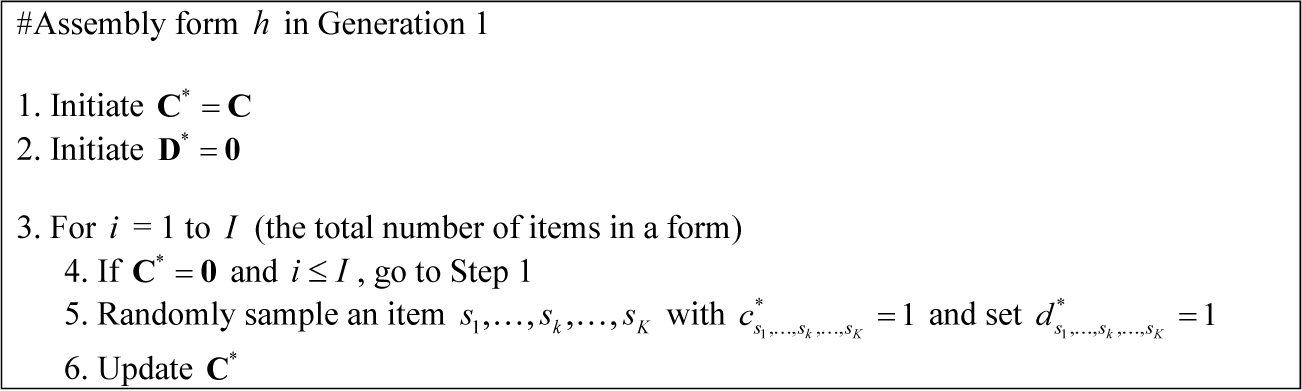


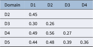
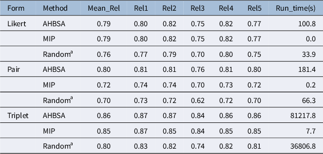
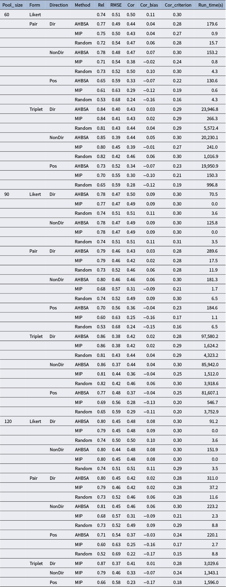
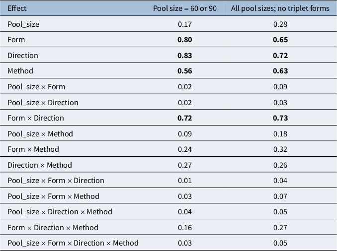

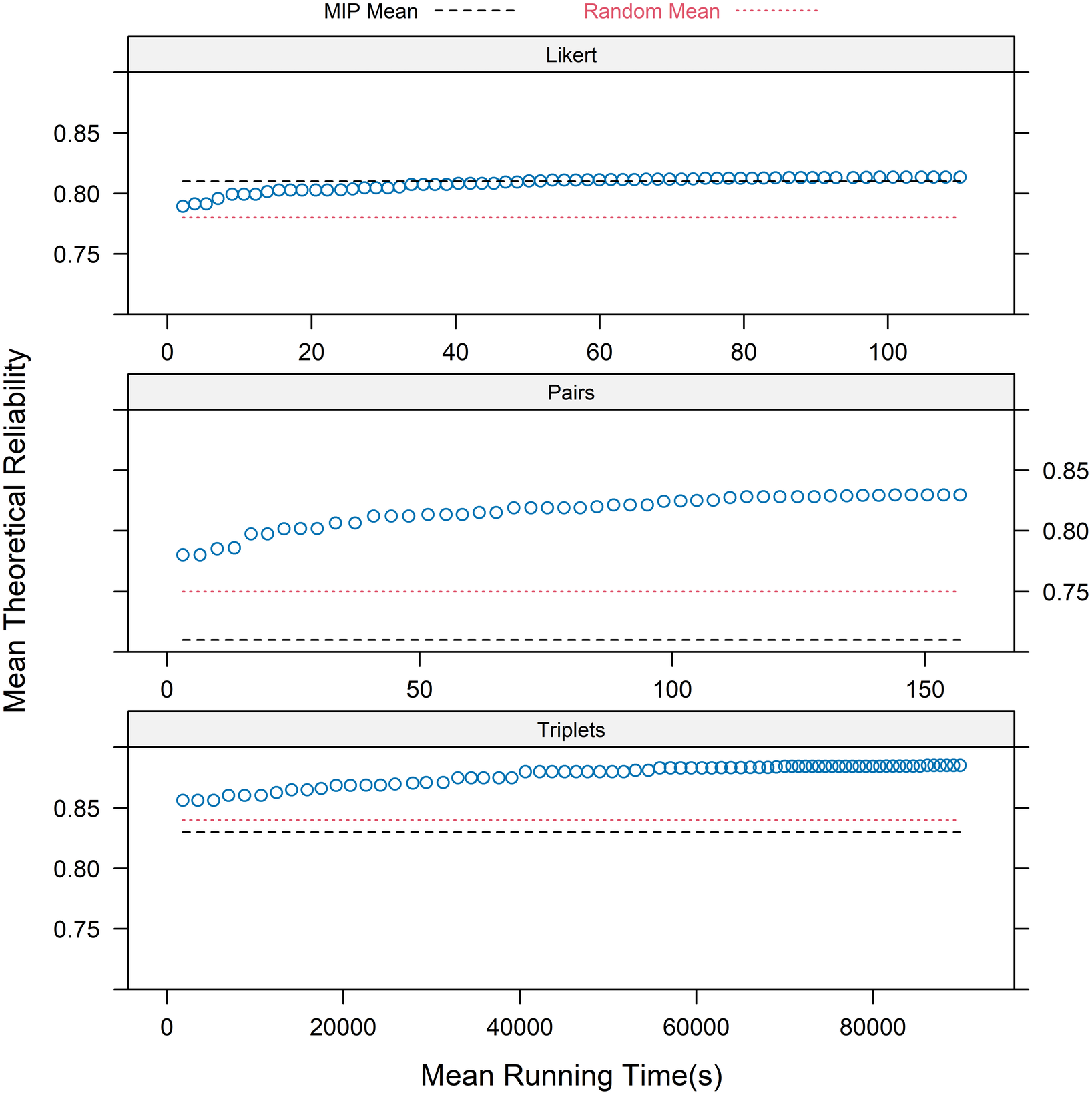
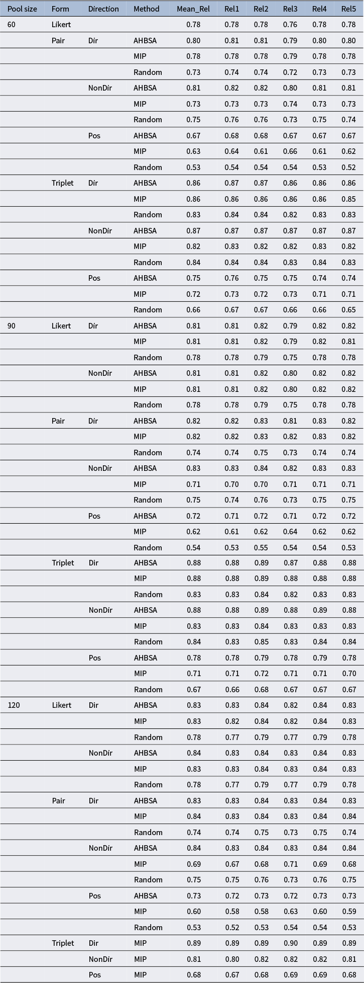

 Open access