Introduction

The Antarctic ice sheet has provided an extraordinary laboratory for a variety of scientific purposes, including measurements of the Earth’s climatological history (Reference PatersonPaterson, 1994), and studies of the early solar system using meteorites collected on the Antarctic surface Reference DoddDodd, 1989. The AMANDA Antarctic Muon And Neutrino Detector Array; Reference AhrensAhrens and others, 2003a, Reference Ahrensb, Reference Ahrensc, ICECUBE Reference Karle, von Feilitzsch and SchmitzKarle, 2002, Radio Ice Cherenkov Experiment; Reference KravchenkoKravchenko and others, 2003a, Reference Kravchenkob RICE and ANITA ANtarctic Impulsive Transient Apparatus collaborations seek to use the solid, large-volume and extraordinarily transparent for wavelengths ϡ00nm ice sheet as a neutrino target. The pioneering AMANDA experiment has successfully demonstrated the viability of englacial neutrino detection through the reconstruction of thousands of atmospheric muon neutrinos Reference NiessenNiessen, 2003 using a photomultiplier tube (PMT) array. ICECUBE plans to extend the coverage and acceptance of AMANDA through a larger-scale (~1 km² effective area) PMT deployment, sensitive to Cherenkov radiation in the near-ultraviolet (250-400 nm) region of the electromagnetic spectrum.

The RICE and ANITA experiments also seek to detect neutrinos interacting in the Antarctic ice sheet. Whereas AMANDA’s sensitivity is maximal for muon neutrinos, the RICE and ANITA experiments focus on electron neutrino detection. This is done by measuring the Cherenkov radiation produced by neutrino interactions in polar ice, albeit at lower frequencies (100MHz—1 GHz) than AMANDA/ICECUBE. The RICE experiment consists of an array of 17 in-ice dipole receivers, deployed at depths of —100 to —350 m, and read out into digital oscilloscopes. Calibration techniques and event reconstruction Reference KravchenkoKravchenko and others, 2003b, as well as results on the neutrino flux at Earth Reference KravchenkoKravchenko and others, 2003a, are presented elsewhere. Although the measurable neutrino flux is primarily due to interactions below the array, radio-frequency (RF) backgrounds due to air showers or above-surface anthropogenic sources require reconstruction of sources viewed through the firn. Similarly, reconstruction of neutrino candidate interactions by the balloon-borne ANITA experiment requires ray tracing through the firn and into the ice itself. In order to have an accurate estimate of the neutrino energy, it is necessary to know the exact location of the neutrino interaction in the ice. Due to bending of rays through the firn, it is therefore important to have an accurate characterization of the variation of the dielectric constant ε with depth in polar ice (Re(ε) = ε’ = n²).

The variable index-of-refraction of the firn has another important experimental consequence, due to the fact that any change in the index of refraction across a boundary introduces non-zero reflections at that interface. The corresponding reflection and transmission coefficients, for the perpendicular and parallel components of the incident electric field (r⊥ and r⊥ and t⊥ and t t⊥, respectively), are given by the standard ‘Fresnel equations for dielectric media’, in terms of the angle of incidence (θ_i) and angle of transmission (θ_t),

Thus, the measured RICE signal strength for above-ice sources, as viewed by below-firn receivers (or vice versa), depends on the degree of variation in the index of refraction. For the case of the balloon-borne ANITA experiment, the dielectric contrast at the surface (i.e. the air–ice interface) determines the critical angle, and therefore also dictates the volume of ice which is visible to the balloon. Measurements of the index-of-refraction at the bottom of the ice sheet, and therefore the strength of the return echo when the ice is probed by ground-penetrating radar (GPR) from the surface, are also used to discriminate between pure ice–rock vs ‘dirty’ ice–rock vs water–ice interfaces. This also has importance in understanding the features beneath the ice-covered surfaces of Jovian moons such as Europa.

Previous Results

The dielectric response of a given medium to an electromagnetic excitation of angular frequency ω is often formulated in an atomic-resonator model Reference HechtHecht, 2001. In such a model, it is not surprising that the index-of-refraction of water varies substantially between the liquid and solid phases, or as a function of impurity. The dielectric properties of ice have been well studied Reference Bogorodsky, Miller, Bentley and GudmandsenBogorodsky and others, 1985. We present below only a subsample of the measurements that have been made thus far. The bulk of the measurements of polar ice properties have been performed in the laboratory using cored samples of Arctic or Antarctic ice, or on laboratory-prepared samples of ice at a given temperature, impurity level and density. Deviations between in situ vs laboratory dielectric measurements can then give information on the impurity content of in situ samples Reference Fujita, Matsuoka, Ishida, Matsuoka, Mae and HondohFujita and others, 2000.

Laboratory measurements

Resonance techniques can be used to make high-precision measurements of ice dielectric response under controlled conditions. Such techniques lend themselves most readily to GHz regime measurements, corresponding to the size scale of typical laboratory samples. In the resonator model, the frequency dependence of n in the 0.1-1 GHz regime is negligible for cold ice; the temperature dependence has been measured in the laboratory to be very small: ε’ = 3:1884 + 9:1T ⁻⁴, with T the temperature in ଌ (Reference GoughGough, 1972; Reference Johari and CharetteJohari and Charette, 1975; Reference Mätzler and Wegmu¨llerMaätzler and Wegmu¨ller, 1987). Over the profile of a typical Antarctic ice core, this corresponds to an expected variation of <1%. A dedicated dielectric profiling device, capable of measuring dielectric properties of ice over a wide frequency range (Reference Moore and ParenMoore and Paren, 1987; Wilhems and others, 1998 Wilhems, 2000, has been used to directly measure the complex dielectric constant over the first 100 m of core B32 Reference Eisen, Wilhelms, Nixdorf and MillerEisen and others, 2003 taken in 1997/98 from Dronning Maud Land, Antarctica, at an elevation of 2900 m Reference OerterOerter and others, 2000. Those data, for both Re(ε) (= ε’) and Im (ε) (= ε"), are reproduced in Figure 1. Shown are the real (refractive) and imaginary (absorptive) components of the dielectric constant over the length of the measured core. At 100 m depth, these measurements correspond to n = √3:0 = 1.732.

Fig. 1.

Complex dielectric constant, measured from core B32 in Dronning Maud Land, from Reference Eisen, Wilhelms, Nixdorf and MillerEisen and others (2003). (a) Ordinary relative permittivity ε’; (b) dielectric loss factor ε", measured at 250 kHz and scaled to 200 MHz, using: ε = ε’ − iε" = ε’ − iσ (ε ₀ ω) −1, where the real part ε’ is the ordinary relative permittivity of the medium, and the imaginary part ε " is the dielectric loss factor. The latter can be expressed as a function of conductivity σ, angular frequency ω and permittivity of vacuum ε ₀ (as indicated) and allows scaling of the absorptive portion of the dielectric constant from kHz to MHz frequencies. Gray horizontal bars indicate dielectric-profiling data gaps. (Reprinted from http://www.agu.org/pubs/sample_articles/cr/2002GL016403/2.shtml.)

Methodology and Experimental Apparatus

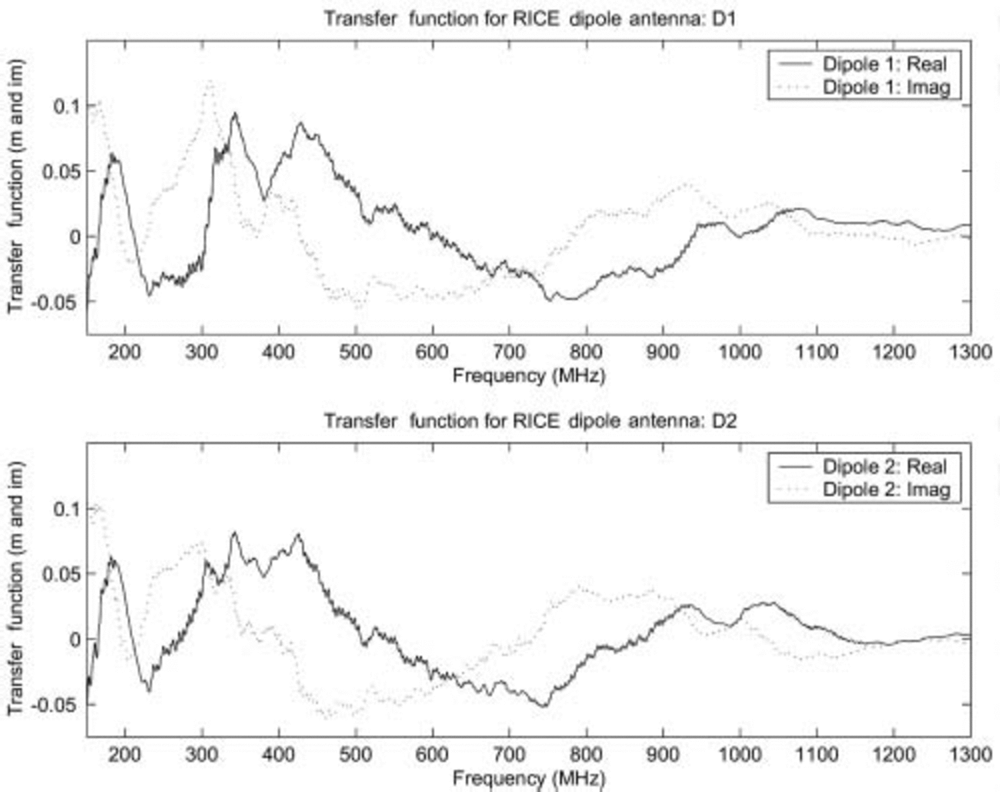
The RICE experiment at the South Pole presently consists of a multichannel array of radio receivers (‘Rx’), scattered within a 200 m χ 200 m χ 250 m volume, at 100−350 m depths. Each receiver contains a 0.3 m long (l = 0.3 m) half-wave dipole antenna, offering good reception over the range 0.2-1 GHz. The peak response of the antenna is measured to be at ~450MHz in air (450MHz/n~250MHz in ice), with a bandwidth Δf/f~0.2. Antenna response can be quantified as a complex transfer function (or effective height) T (m); given an incident electric field , the voltage V induced at the output of the antenna is given by . For a half-wave dipole antenna, the longest-wavelength resonance is expected at λ = 2l; the magnitude of the effective height at resonance is expected to be of order l/π (Reference KrausKraus, 1988; Reference BalanisBalanis, 1997). Our measured antenna response is observed to be roughly reproducible from antenna to antenna and (roughly) consistent with expectation (Fig. 2).

Fig. 2.

RICE dipole transfer function, measured in air for two typical RICE dipoles.

The signal from each receiver antenna is immediately boosted by a 36 dB in-ice amplifier, then carried by ~300m coaxial cable to the surface observatory, where the signal is filtered (suppressing noise below 200MHz due to both AMANDA phototubes and continuous-wave backgrounds from South Pole station at 149 MHz), re-amplified (either 52 or 60dB gain), and split into two copies. One copy is fed into a (LeCroy Corporation) CAMAC electronics crate from which, after initial discrimination (using a LeCroy 3412 discriminator), the signal is routed into a Nuclear Instrumentation Methods (NIM) electronics crate where the trigger logic resides; a hit time is subsequently recorded by a LeCroy 3377 Time-to-Digital Converter (TDC) module for each receiver channel above threshold. The typical threshold is approximately a factor of five larger than the ambient thermal noise background σ_kT. The quoted timing resolution of the TDC module is 0.5 ns; this is verified in studies of the TDC 3377 using identical signals injected into two different channels of the TDC and comparing the recorded times in the two different channels. The other copy of the analog signal from an antenna is input to one channel of an HP54542 digital oscilloscope, where waveform information is recorded. Also deployed on the surface are three large transverse electromagnetic (TEM) horn antennas which are used to suppress surface-generated noise. Signals recorded in the TEM horns generate an inhibit signal which will blank out the data-acquisition system for the subsequent 3 μs. For RF backgrounds generated on the surface, we expect hits to be first recorded in the TEM horns and then later (within 3μs) in the englacial dipole antennas.

Detector Array Geometry

The status of the current array deployment is summarized in Table 1 and Figure 3. Further details on detector geometry, deployment and calibration procedures are presented elsewhere (Reference KravchenkoKravchenko and others, 2003b).

Table 1.

Location of RICE radio receivers. We have adopted the coordinate system convention used by the AMANDA collaboration. The transmitter is lowered into hole B4

Fig. 3.

Three-dimensional view of RICE receiver antenna array.

For most of the measurements discussed in this paper, the transmitter was located at various depths in hole B4 (which also contains the channel 11 receiver), and broadcasting to the entire RICE receiver array. The Martin A. Pomerantz Observatory (MAPO, South Pole) building houses hardware for several experiments, including the RICE and AMANDA surface electronics, and is centered at (x~40m, y ~ −30 m) on the surface. The AMANDA array is located approximately 600m (AMANDA-A) to 2400m (AMANDA-B) below the RICE array in the ice; the South Pole Air Shower Experiment (SPASE) is located on the surface at (x ~ —400 m, y ~ 0 m). The coordinate system conforms to the convention used by the AMANDA experiment; grid north is defined by the Greenwich Meridian and coincides with the +y direction in the figure. The geometry of the receivers used for this measurement is also presented in Table 1.

Experimental Procedure

In December 2002, two of the dry holes (B4 and B2, respectively) were uncovered by clearing away (i.e. shoveling) the 1.2-1.5 m deep snow cover which had accumulated in the intervening 4years. The holes were found to be generally in the same condition as when they had originally been drilled. After hole B4 was uncovered, a ~300m length of coaxial cable was used to connect a transmitter (Tx) to a high-amplitude, fast rise-time pulse generator (AVTECH model AVIR-1-C) located within MAPO. One of the 20 oscilloscope input channels (four inputs on each of the five HP54542 digital oscilloscopes) was used to monitor the AVIR-1-C pulse-generator input and also to provide the overall start time (t ₀) for the recorded event. Figure 4 shows the monitored pulser signal (t ₀) for four successive events, indicating the reproducibility of the pulser output, as well as the fast rise time of the output signal.

Fig. 4.

V(t) trace for AVIR-1-C pulser input for transmitter signal used in this experiment, for four successive events. Reproducibility of signal t0 at t = 1981.5 ns is evident. Horizontal binning is in units of 0.5 ns.

Fig. 5.

Geometry of initial measurements. The transmitter (Tx) is connected, via coaxial cable, to a pulse generator or a continuous-wave generator in the MAPO. The transmitter broadcasts to one of the RICE dipole antennas (located in-ice). The angle θ is measured relative to the z axis, and is the angle of incidence used in the Fresnel equations and for ray tracing. With this definition of angles, the expected dipole antenna beam pattern is then given by: E (θ) ~ sin θ.

After connecting one copy of the pulse generator to the dipole transmitter via the coaxial cable, the transmitter was lowered into hole B4. At either 5m (-32m<z _Tx) or 10m (zTx<-132 m) depth increments, a pulser signal (Fig. 4) was broadcast from the transmitter to the RICE receiver array, and signal arrival times in the receivers recorded (Fig. 5). (To check the reproducibility of our measurements, data were also recorded as the transmitter was later raised out of the hole.) Each pulser signal afforded two measurements of the index of refraction:

1. 1. the index of refraction as a function of depth (n (z)) was inferred by determining the transit time difference to a particular receiver between successive transmitter locations with ti the transit time corresponding to the transmitter at source location i, tj the transit time corresponding to the transmitter at source location j, the vector defining the position of the transmitter at source location the vector defining the position of the transmitter at source location j, the vector defining the position of the (stationary) receiver, and c the velocity of light in a vacuum);

2. 2. the ‘mean’ index of refraction (〈n(Δz)〉), averaged over the distance from the transmitter to any receiver, was inferred knowing the time of the output pulser signal for each event (t ₀), the cable time delay between generator and transmitter (t _Txgen), the cable time delay between receiver and data-acquisition system (DAQ) (t _Rx, DAQ), and the time recorded for the ith receiver at the DAQ (t _Rx, _i ) as:

   

The former technique has the virtue of mapping out the index-of-refraction dependence on depth (n (z)); the latter technique has the virtue of being less sensitive to transmitter location uncertainties as the transmitter is being lowered.

At each transmitter location, 20 successive transmitter pulses were broadcast. For each transmitter pulse, an 8.192 ms waveform (sampled at 2 GSa s^–1) was captured in the digital oscilloscope, for each receiver. As noted before, the t ₀ of the transmitter signal was also recorded in one of the oscilloscope channels, to monitor possible timing shifts within the DAQ. Figure 6 illustrates the reproducibility of the receiver waveform for four typical samples corresponding to a given transmitter–receiver configuration.

Fig. 6.

Receiver waveforms recorded from channel 2 for four transmitter samples; for these data, the transmitter was located at –150m depth. Received signals are observed to be reproducible from event to event.

n (z) Determination From Relative Receiver Hit Times

Figure 7 shows the migration (with time) of the direct-path hit times recorded in a typical channel (in this case, channel 2) of the RICE DAQ as the transmitting antenna is lowered into hole B4 (surface-reflected signals are discussed below). Several features are clear from this figure: (a) visually, the rise time of the signal can be measured to within ±1 ns (two bins); (b) the signal shapes are not exactly reproducible at the various transmitter depths, suggesting ray-tracing complications due to the varying index of refraction or perhaps cross-talk effects; (c) although the angle of incidence relative to the receiver is changing substantially, the near-constancy of the peak amplitude suggests (given the sharp dependence of the Fresnel reflection coefficients with angle of incidence) that reflections off possible internal layers are not large.

Fig. 7.

Channel 2 waveforms recorded for transmitter at three different source depths. Horizontal axis is counts, in 0.5 ns bins. Vertical scale is recorded voltage. Although depths are equally spaced (–160, –90 and –20 m), the hit times are not uniformly spaced since the receiver is not vertical with respect to the transmitter.

The index of refraction is directly obtained from the electromagnetic wave propagation speed. At each transmitter depth, we record the hit time (discussed below); the variation in receiver hit times with transmitter depth is shown in Figure 8, for 13 receivers. The different shapes of these curves result primarily from differences in geometry between the various Tx-Rx pairs. (Note that each receiver can, in principle, be used to determine the index of refraction in the vicinity of the transmitter; in practice, the receivers which are closest to the axis of hole B4 (i.e. directly below or above) are geometrically best suited to make this measurement.) For each transmitter location, the electromagnetic wave propagation speed is directly obtained from the slopes in this figure, and can therefore be translated into an index-of-refraction profile, n (z).

Fig. 8.

Transmitter depth location vs recorded receiver hit times, for 13 different receivers. Channels are as indicated in the legend. The slope of each curve gives one determination of n (z).

Before presenting numerical results, however, it is necessary to briefly consider the trajectories followed by rays in the ice, and possible complications due to our simplifying straight-line ray assumptions.

Ray-tracing considerations

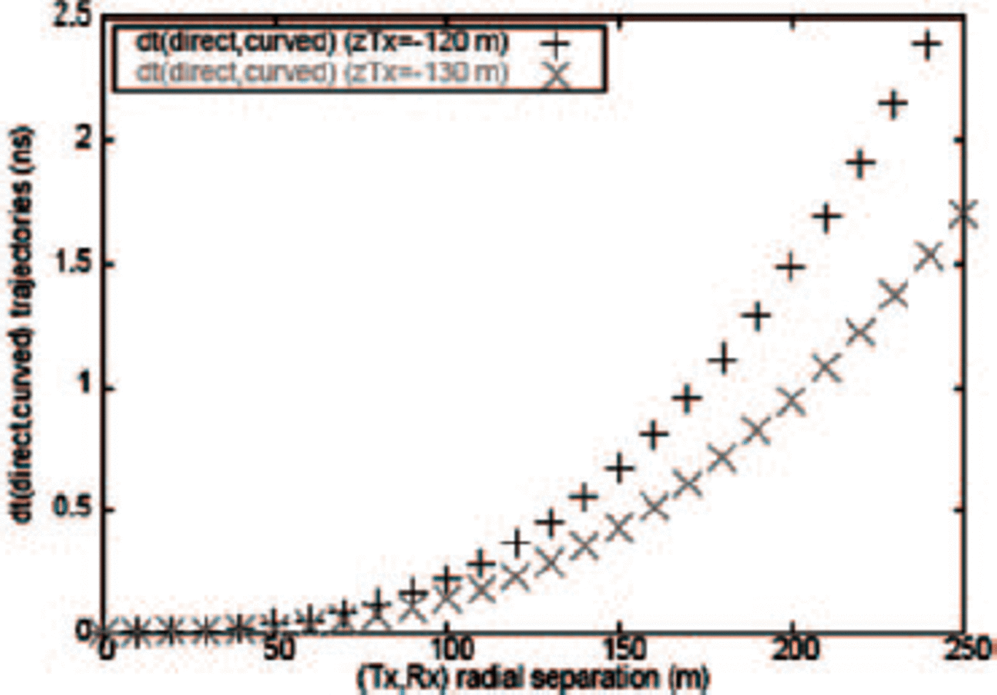
The trajectory of electromagnetic waves is determined by Fermat’s least-time principle; a straightforward derivation can be used to obtain dö/dl = — (∂n/∂z)(sinθ/n), with θ the angle of incidence on the horizontal plane, dl a differential path length along the ray’s trajectory, and ∂n/∂z the gradient in the index-of-refraction with depth (the objective of this measurement). This expression leads to the (counterintuitive) conclusion that even a ray directed horizontally along a contour of constant index of refraction will begin to bend into the region of higher index of refraction. Assuming a transmitter at -170 m depth, below the nominal firn-ice transition, Figure 9 displays the expected ray tracing (based on our measured n(z) profile) up to a radial distance of 400 m from the source. Since, for our experiment, the transmitter-receiver distances are typically <250m, such curvature effects are slight. Relevant to our experiment is the possibility that the effect of curvature on the difference of transit times between two source locations 5-10 m apart is larger than our our typical measurement error (~1 ns). Figure 10 shows two sample trajectories, one connecting a hypothetical transmitter at zT_x = — 120 m to a receiver at z _Rx = — 120 m, and another for z _Tx = — 130 m and z _Rx = —130 m (note the aspect ratio between the x and y scales in the figure). Next ()Fig. 11, along the trajectory of the rays shown, we can calculate the difference dt between the simple direct path vs the fully ray-traced path, as a function of the radial separation between transmitter and receiver for two cases. We observe that the correction (σ_ray) for measurements made at successive transmitter locations (the difference between the two curves) is typically of order 0.5 ns or less; our conclusion is qualitatively consistent with previous estimates that the error in wave speed (as obtained from an x ² vs t ² plot) assuming straight-line ray tracing will be π.5% (Reference Bogorodsky, Miller, Bentley and GudmandsenBogorodsky and others, 1985. This correction is neglected for the subsequent analysis, but included in our determination of the total error σ_tot.

Fig. 9.

Trajectories of rays (in the (r;z) plane) expected from a transmitter broadcasting from a depth of z = -170 m.

Fig. 10.

Expected curvature of two rays connecting in-ice transmitter to in-ice receiver, with receiver and transmitter both at either-120 or-130 m in depth. Note the 10:1 aspect ratio of x_vs y scales.

Fig. 11.

Magnitude of time correction between transit time calculated for straight-line path vs transit time calculated with full ray tracing, along the trajectories shown in Figure 10.

We point out that this correction is, unfortunately, nonlinear: Suppose we take measurements in a receiver Rx, below the firn, at two different transmitter locations T _xi and Tx_j. Measurement i is made with the transmitter in the firn, and measurement j is made with the transmitter below the firn; for each measurement there is a corresponding straight-line distance di or dj to the receiver. No ray-tracing corrections are applicable for Tx _j → Rx; however, for Tx _i → Rx, the actual curved trajectory di is longer than the straight-line trajectory. Since we have used c/n = (di − dj)/ (ti − t_j ), with t_i − t_j the measured hit-time difference, inserting the true (larger) curved path length di has the effect of reducing the calculated value of n. This is expected since the curved trajectory, by Fermat’s principle, preferentially samples shallower, lower index-of-refraction ice. By neglecting this effect, we therefore slightly overestimate both the index of refraction and the appropriate measurement depth. To some extent, these two effects tend to offset each other.

Measurement Uncertainties

Known uncertainties arise from the following sources:

1. 1. The temperature dependence of the index of refraction of cold ice has been measured, although it has been shown to be a small (~1%) effect, from 08C to -608C (Reference GoughGough, 1972; Reference Johari and CharetteJohari and Charette, 1975; Reference Mätzler and Wegmu¨llerMa¨tzler and WegmÜller, 1987). Over the first 150 m of the ice, the temperature variation is expected to be <5°C. The corresponding effect on measurements taken from any two successive transmitter locations is therefore expected to be insignificant.

2. 2. There is some uncertainty associated with discerning the actual hit time. To minimize this, the 20 events recorded on each receiver from each transmitter height were added, in order to enhance signal-to-noise, and the signal arrival times were also extracted by visual inspection of the summed waveforms. Alternately, the receiver arrival times can be determined from various software algorithms. The simplest algorithm simply picks out the first 6σ_kT excursion in a waveform, where σ _kT is the rms noise in the waveform outside the signal region, dominated by thermal noise. More sophisticated algorithms calculated the χ ² between the receiver signal and the expected signal shape (knowing the transfer function described previously), and selected the time in the waveform which gave the lowest χ ², or selected the first time in the waveform for which at least four of any eight sequential samples corresponded to >4σ_kT. ‘Good’ data were required to satisfy the requirement that the variation σ_hit between the four algorithms was ρ ns.

3. 3. Since the transmitter depths were determined using the length markings directly on the cable, which was marked in both 1 ft and 1 m intervals, additional measurement uncertainties arise from transmitter depth uncertainties (<0.5 m) at each transmitter location. Survey errors in the locations of each receiver are estimated at ~1 m per receiver.

Results

We have attempted to obtain an aggregate estimate of n (z) by:

1. 1. averaging the raising-transmitter plus lowering-transmitter datasets;

2. 2. averaging all highest-quality data from all possible channels, where the contribution to the final average from each channel was weighted by geometry and favoring nearly vertical receiver channels (the error was assessed here as 1/σ² _geometry = (t_i − t _{i + 1}), where t_i and t_{i + 1} are the calculated transit times for the measurements i and i + 1. Cases where the times are approximately the same for two successive measurements, i.e. the receiver and transmitter are at approximately the same depth, are therefore substantially deweighted) and reproducibility of the extracted hit time (favoring cases where the software algorithm found the same hit time for all of the 20 events taken at one transmitter location). An rms error, σ₂₀, was determined for the 20 measurements, and a requirement that this rms value be ρ ns (two waveform samples) was imposed, after requiring consistency among the four hit-time algorithms;

3. 3. reducing the effect of uncertainties in the transmitter locations by re-obtaining averages taking the data obtained for 10-20 m distance differences (rather than 5-10 m) between successive Tx broadcasts. That is, we calculate n (z) using t _Txi relative to t _Tx, _i +2 rather than relative to t _Tx, _i +₁ and therefore reduce the ratio of the time error arising from uncertainties in the transmitter location relative to the difference in propagation time between successive measurements. We would expect this procedure to correct for cases where the transmitter may have been slightly higher or lower than recorded for the intervening measurement.

The difference between these coarse-grained measurements and the default finer-grained measurements contributed another error σ _Δz . Because the index-of-refraction profile is non-linear, the coarse-grained measurements tend to underestimate the index of refraction in the vicinity of the transmitter, so these measurements are not used directly, but are only used to determine an associated error. We then calculate a total error σ_tot , which is the inverse quadrature sum of all the errors cited above, at each transmitter location Figure 12 shows the result of this procedure, and also includes data obtained by broadcasting horizontally between a transmitter being lowered into hole B4 and a receiver being lowered into hole B2. Also included are measurements derived from the ‘mean’ n (z) values obtained using absolute t ₀ measurements, which average over the n (z) profile between transmitter and each receiver, as well as comparisons with the predictions of the Schytt model for density and n(z) = 1 + 0.86ρ(z), assuming alternately that the ice-firn transition occurs at z = -115 m and at z = -130 m.

Fig. 12.

Final fitto index-of-refraction data, combining information from all active receiver channels, and combining both up-going and down-going transmitter datasets. Statistical errors only are shown; inclusion of the systematic errors (estimated 4% at each point) would reduce the significance of the apparent ‘dip’ in the data points relative to the fitted curve around z~ —80 m to below 2σ significance.

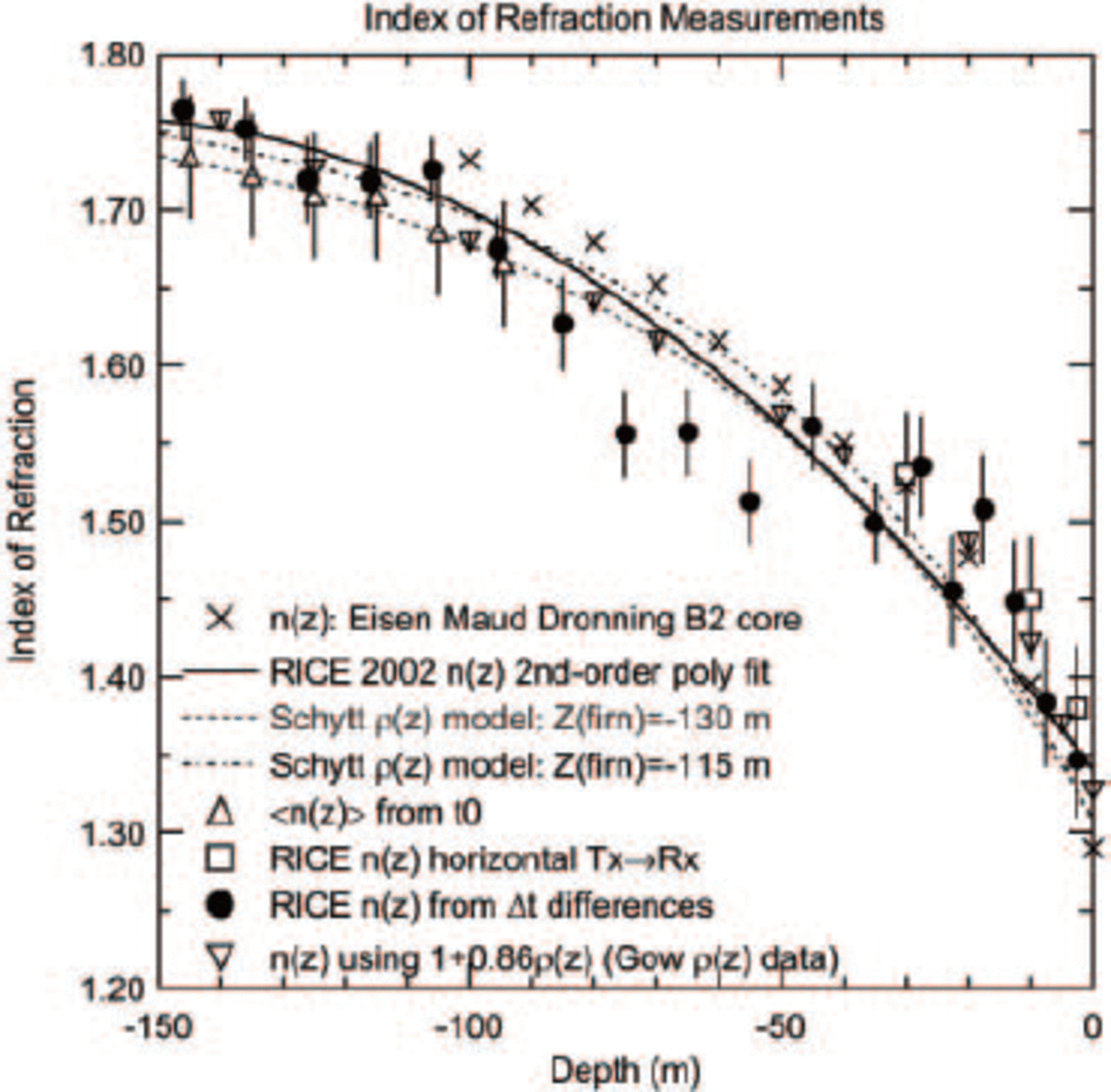
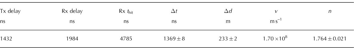
The RICE data points are fit to a second-order polynomial (n (z) = 1:324 − 5:2854z − 21:865z ² − 39:058z ³; z is in km for this parameterization), with the assumption that the value of index of refraction at large depths approaches a constant. We obtained an estimate of that asymptotic value by broadcasting from the deepest buried RICE transmitter (x = −85 m, y = 8m, z = −200 m) down to the deepest buried RICE receiver (channel 15); both of these antennas are presumably well below the firn-ice transition. Those data are presented in Table 2, and are included in our fit.

Table 2.

Data used to extract asymptotic value of n(z)

This asymptotic value is in fair agreement with the accepted value of 1.78, as obtained by several measurements (Reference EvansEvans 1965);(Reference Gudmandsen and WaitGudmandsen, 1971);(Reference Hempel, Thyssen, Gundestrup, Clausen and MillerHempel and others, 2000). The confidence level of the fit to all the RICE data points in figure 12, using just the previously tabulated errors (σ_tot), is rather small (3.1%). In order to achieve a confidence level of 50% requires an error, per data point, of 4%. We take this to be a conservative estimate of the overall (systematic plus statistical) error, point-to-point, on the measurement. Our data favor a non-linear variation of index of refraction with depth, albeit only slightly: fitting n (z) to a linear form (n (z) = c ₀ + c ₁ z) results in an increase in X²/degree-of-freedom of only 0.15.

Cross-Checks

Comment on Reflections

The possibility of multiple paths connecting transmitter to receiver suggests the possibility that we might observe after-pulses (or ‘double pulses’). The simplest reflected path is expected to be a path which corresponds to an upward-directed ray from a transmitter, bouncing off the top surface ice-air discontinuity, and back down to a buried receiver. We have searched for reflections by looking for after-pulses in the captured waveforms after the initial hit times as shown in Figure 13. In the ‘surface reflection’ model, we expect the time delay between the first and second pulses to increase with transmitter depth. We observe after-pulses in all channels. These measurements also offer a check of our ray-tracing algorithm. Figure 14 compares the expected time delay between the initial pulse and the after-pulse with the observed time delay, for four different channels. Within our ability to visually discern the hit time of the after-pulse, we find reasonable agreement between our ray-tracing model and the data. In principle, a timing analysis and an amplitude analysis (using the Fresnel equations) could be used to independently determine the index-of-refraction profile up to the surface, and the index-of-refraction discontinuity at the surface, respectively. Such efforts are currently in progress.

Fig. 13.

Successive voltage signals (corresponding to increasing depths) observed for transmitter broadcasting to channel 0 of the RICE data-acquisition system. Note the systematic increase in time delay between primary and after-pulse as the transmitter depth increases. Horizontal scale is in units of 0.5 ns.

Fig. 14.

Modeled vs measured values of the expected time delay between direct-path pulse and after-pulses due to surface reflections observed in our transmitter data.

Comment on Internal Layer Reflections

Layers can arise as a result of episodic events (e.g. dust or acid layers due to volcanic eruptions) or annual processes, including thin surface crusts which form in the summer, constituting a discontinuity in density. Layers of the latter type should become less important with depth as the ice approaches its asymptotic density. Anisotropies in the crystal structure of the ice may also constitute a discontinuity. Nearer to the coast, brine infiltration can also result in stratified layering. However, this is expected to be negligible at the South Pole. Precise study of layers requires extremely sensitive receivers and, in the case of annual layering, the ability to distinguish density differences of order 1-10cm apart (<1 ns) in the ice. Interferometry or pulse modulation techniques can also be used to probe layering, provided the interferometer is sensitive to 1 ns time-scales. Such exacting requirements have hampered a complete understanding of internal layering thus far using GPR data. In addition to discrete layers, quasi-continuous λ⁻⁴ Rayleigh scattering off air bubbles in unenclathrated ice has been considered quantitatively (Reference Smith and EvansSmith and Evans, 1972), resulting in a ‘worst-case’ estimate of an attenuation loss of 0.7λ⁻⁴dB per 100 m.

Reflections off internal layers can modify the ray tracing required in our extraction of n (z). Although we can detect the surface reflections shown in Figure 13, we have insufficient sensitivity to directly observe reflections off internal layers. Such layers have previously been observed (using GPR) as low-power (typically, -60 to -80 dB) returns from within and below the firn. (Reference Bogorodsky, Miller, Bentley and GudmandsenBogorodsky and others, 1985). suggest an ‘equivalent-layer’ model consisting of 1 mm thick layers spaced ~1-10m apart, with a dielectric contrast Δε/ε = 0.002, or An/n = 0.001 between successive layers. We have attempted to test such a model by plotting the amplitude of the received signals (in units of σ_kT), as a function of the angle of incidence of rays traced from the transmitter, as it is being lowered, to a receiver (for simplicity, we have assumed straight-line trajectories for this exercise). Although layers can ‘trap’ signal, possibly resulting in an amplified received signal, we expect that such trapped signals may (depending on the incident angles) arrive at the receivers asynchronously with the primary hit, and neglect such effects in our analysis. We also neglect any second-order reflections, i.e. transmission through layer 1 followed by reflection off layer 2 (with possible subsequent interference effects). Figure 15 displays the Fresnel-derived transmitted amplitudes for 1 m layering, assuming a density contrast of 0.001 for successive layers, as a function of the incidence angle θ. Curves are presented for various values of vertical displacement d z between Tx and Rx. In this scheme, traversal of multiple layers results in a multiplicative, rather than a linear, loss of signal amplitude (in practice, there would be ‘thin-film’-type interference between the signals arriving from (multiple) reflections within the ice; we neglect such effects for the purpose of this simplified analysis). The model includes the dipole antenna beam pattern (E (θ) ~ sin θ, or, equivalently, E (∅) ~ cos ∅), and also takes into account the 1/r loss of amplitude with distance from receiver, to allow a direct comparison with data. Figure 16 shows the ensemble of all recorded data (all recorded signals for all receiver data, in units of kT thermal noise): for values less than the threshold predefined for ‘good’ hits in this analysis (Signal > 22.5σ_kT), the times are considered unreliable and are not used in the index-of-refraction calculation. Such amplitudes are assigned a value of zero in Figure 16a. If there are significant losses due to the reduced Fresnel transmission amplitudes at ‘glancing angles’, we would expect to see a reduction in the average signal strengths recorded as cos θ → 0, as well as an increase in the number of recorded signals entered as zeroes. Our data show no dramatic decrease of signal as cos θ → 0 (θ → π/2), as would be expected in the multiple scattering-layer model depicted in Figure 15. shows a zoom of the region around cos θ ~ 0 using receivers which sample depths both above and below the transmitter. Again, our data do not indicate significant signal loss due to internal reflections. This is perhaps not entirely unexpected: since we are in a regime where λ ≫ t _layer, with t _layer the physical thickness of each layer, one might anticipate mitigation of internal scattering effects.

Fig. 15.

Predicted transmission coefficient, as a function of incident angle, and vertical displacement of transmitter relative to a receiver.

Fig. 16.

(a) Raw peak receiver amplitude data recorded for all Tx → Rx combinations, as a function of angle θ. If the recorded receiver amplitude is <22.5σ_kT, a value of zero is entered in this plot. (b) Zoom of data recorded in the region cos θ ≈ 0, where Fresnel losses off possible internal layers should be maximal. Note that positive (negative) values of cos θ correspond to cases for which the transmitter is higher (lower) than the receiver; for the Monte Carlo simulation shown in Figure 15, we have only simulated geometries for which the transmitter is higher than the receiver.

Comment on Birefringence

We note that, in principle, the ice can be birefringent, this birefringence being either ‘linear’ (linear propagation velocities different along two perpendicular axes in the ice; presumably the symmetry axis is defined by gravity in the upper few hundred meters at the South Pole) or ‘circular’ (in the case where there is some rotational asymmetry in the crystal structure, for which the propagation velocities of the left- and right-circular polarizations will differ). Since both transmitter and receiver have the same polarization axis (antennas are oriented vertically within the ice holes), we are insensitive to linear birefringent effects. Since circular birefringence results in a separation between the left- and right-circular polarizations, and a rotation of the plane of polarization as the signal moves through the ice from the transmitter, we would expect that the received signal strength would depend on the orientation of the polarization axis at the location of each receiver. The fact that the signal received from a transmitter by each receiver does not obviously show such effects provides circumstantial evidence that circular birefringent effects are not large (Reference KravchenkoKravchenko and others, 2003b).

Conclusion

We have used the RICE array at the South Pole to measure the index of refraction through the firn. We obtain an index-of-refraction profile (n (z)) which qualitatively agrees with that extrapolated from direct laboratory studies of the electrical properties of ice cores. We are also consistent with the expected correlation of n(z) with ice density ρ. We note that, since the firn-ice transition corresponds to ρ ~830kgm–³, we can use the linear dependence of the refractive index on density to infer a firn-ice transition depth of z ~ − 100 m from our data, although values down to z ~ −130 m are allowed, given our errors. Our results have implications for experiments which rely on the detection of radio waves propagating through the firn. This includes GPR probes of the ice sheet, which translate a measured time delay into a depth, and also includes experiments based on the detection of radio waves from neutrino-induced electromagnetic showers in the ice.

The measurement technique, however, has limitations due to the finite bandwidth of the antennas and data-acquisition system we have used, which smears the measured signal onset in the time domain. An improved in situ measurement would utilize higher-bandwidth electronics, thus permitting higher-resolution software techniques (matched filters) to improve the timing granularity well beyond the intrinsic sampling time of the measurement hardware.

In the austral summer 2003/04, efforts were focused on measurements of the imaginary (absorptive) component of the dielectric constant. Results on those measurements are currently in preparation.