


1. Introduction
The Antarctic ice sheet plays a crucial role in global climate processes, and the stability of its ice shelves is considered a major source of uncertainty in predicting future sea level (Hanna and others, Reference Hanna2020; Fox-Kemper and others, Reference Fox-Kemper2021). Floating ice shelves occur along 75% of the Antarctic coastline, forming a vital connection between the ice sheet and the ocean (Ingels and others, Reference Ingels2021) and their dynamic changes are critical in assessing the ice sheet mass balance and its contribution to sea level rise (Shepherd and others, Reference Shepherd2018). Ice shelves are composed of meteoric ice from two sources, ice flowing from grounded glaciers and the ice sheet and new snow accumulation on the upper surface, together with marine ice formed mainly through the accretion of frazil ice crystals at the ice–ocean interface (Jansen and others, Reference Jansen, Luckman, Kulessa, Holland and King2013).
Marine ice is the product of thermohaline circulation at the bottom of ice shelves (Robin, Reference Robin1979), which is driven by the ice pump mechanism (Lewis and Perkin, Reference Lewis and Perkin1986; Bombosch and Jenkins, Reference Bombosch and Jenkins1995) in which cool and relatively fresh water formed by ice melting at depth rises buoyantly toward the shelf front. Ice crystals may form in the rising water where it becomes supercooled as the ambient pressure declines. This supercooled water and the crystals it produces are the sources of marine ice. The accumulation of marine ice alters the thickness of the ice shelf and the bottom structure, reducing the net mass loss of ice shelves and affecting ice flow and circulation at the bottom of the ocean (Williams and others, Reference Williams, Warner and Budd2002; Craven and others, Reference Craven, Allison, Fricker and Warner2009). Moreover, marine ice can modulate the stress field and inhibit crack propagation, which impacts the stability of ice shelves (Jansen and others, Reference Jansen, Luckman, Kulessa, Holland and King2013; Kulessa and others, Reference Kulessa, Jansen, Luckman, King and Sammonds2014; Hillebrand and others, Reference Hillebrand, Conway, Koutnik, Martín, Paden and Winberry2021; Harrison and others, Reference Harrison, Holland, Heywood, Nicholls and Brisbourne2022). Therefore, accurately describing the spatial distribution of bottom marine ice is crucial in dynamically modeling the evolution of ice shelves and assessing their instability.
Marine ice has been detected beneath several ice shelves in Antarctica (Neal, Reference Neal1979; Thyssen, Reference Thyssen1988; Craven and others, Reference Craven2004; Holland and others, Reference Holland, Corr, Vaughan, Jenkins and Skvarca2009), with the Amery Ice Shelf (AIS), the largest ice shelf in East Antarctica, being one of the key focuses of research. The presence of marine ice under the AIS was first observed in a borehole during a polar expedition in 1968 (Morgan, Reference Morgan1972). Fricker and others (Reference Fricker, Popov, Allison and Young2001) subsequently mapped the distribution of marine ice using satellite laser altimetry, airborne radio-echo sounding (RES) measurements and the hypothesis that differences between RES-observed thickness and thickness predicted using Archimedes’ principle and the surface height must be due to an unobserved layer of marine ice. The Australian Amery Ice Shelf Ocean Research (AMISOR) project then investigated the internal structure of the ice shelf and the interaction between the ice base and the ocean through six hot-water-drilled boreholes (AM01–AM06) (Fig. 2; Allison and Craven, Reference Allison and Craven2000; Craven and others, Reference Craven, Warner, Galton-Fenzi, Herraiz-Borreguero, Vogel and Allison2014). However, previous inversion or measurement results were constrained by the detection limitations of airborne radar, such as the uncertainties inherent in the early analogue, lower geolocation accuracy and limited depth resolution (Popov, Reference Popov2022), all of which introduce error in marine ice-thickness estimates. In situ observations are sparse and there have been no follow-up measurements of marine ice thickness on the AIS since Fricker and others’ (Reference Fricker, Popov, Allison and Young2001) pioneering work. Meanwhile, global warming has progressed, and changes in polynya formation and ocean circulation on the continental shelf are linked with enhanced ice-shelf melt and delayed formation of dense water (Tamura and others, Reference Tamura, Ohshima, Fraser and Williams2016; Aoki and others, Reference Aoki2022; Jordan and others, Reference Jordan, Gudmundsson, Jenkins, Stokes, Miles and Jamieson2023; Gu, Reference Gu2024). A new assessment of the marine ice conditions beneath the ice shelf with contemporary equipment will improve the thickness estimate and improve understanding of AIS processes and change.
Since 2015, the Chinese National Antarctic Research Expedition (CHINARE) has used its ‘Snow Eagle 601’ fixed-wing airborne platform to conduct a comprehensive suite of aerial observations as part of the ongoing International Collaborative Exploration of the Cryosphere by Airborne Profiling (ICECAP) project. ICECAP observations include gravity, RES and laser altimetry in East Antarctica (e.g. Cui and others, Reference Cui2020). These observations have yielded the latest physical detection data for the AIS. Yang and others (Reference Yang2021) used ICECAP data to infer seafloor bathymetry and water column thickness under AIS, and explored the potential effects of ice cavity geometry on ocean circulation beneath the ice shelf. Preliminary estimates of marine ice accretion were suggested in two earlier explorations, utilizing the hydrostatic equilibrium method (e.g. Maylath and others, poster presented in AGU Fall Meeting 2018, 2018; https://agu.confex.com/agu/fm18/meetingapp.cgi/Paper/460707). However, these results relied on sparse observational data, and the possible distribution of marine ice was not further investigated.
In this study, we provide a new estimation of the spatial distribution and thickness of marine ice under AIS based on the newly acquired RES data collected during the CHINARE seasons (2015–19). We accomplish this using the surface elevation from satellite observation and the thickness of meteoric ice measured from the above RES data by assuming hydrostatic equilibrium. We then compare the hydrostatic equilibrium results with marine ice-thickness estimates based on the assumption of mass conservation of ice shelves and further estimate the error of the results. Furthermore, we assess the reliability of the results in combination with ice-thickness data obtained from in situ boreholes.
2. Methods and Data
2.1. Hydrostatic equilibrium
For a free-floating ice shelf, a simple relationship between surface elevation  $h$ (relative to sea level) and thickness $H$ (Fricker and others, Reference Fricker, Popov, Allison and Young2001) is given by the hydrostatic equation:
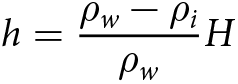 \begin{equation}h = \frac{{{\rho _w} - {\rho _i}}}{{{\rho _w}}}H\,\end{equation}
 where  ${\rho _w}$ and ${\rho _i}$ are the column-averaged densities of seawater and ice, respectively. In the presence of marine ice accretion at the bottom of the ice shelf, the vertical structure of the ice shelf is composed of an upper layer of meteoric ice and a lower layer of marine ice:
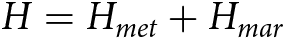 \begin{equation}H = {H_{met}} + {H_{mar}}\,\end{equation}
 in which  ${H_{met}}$ and
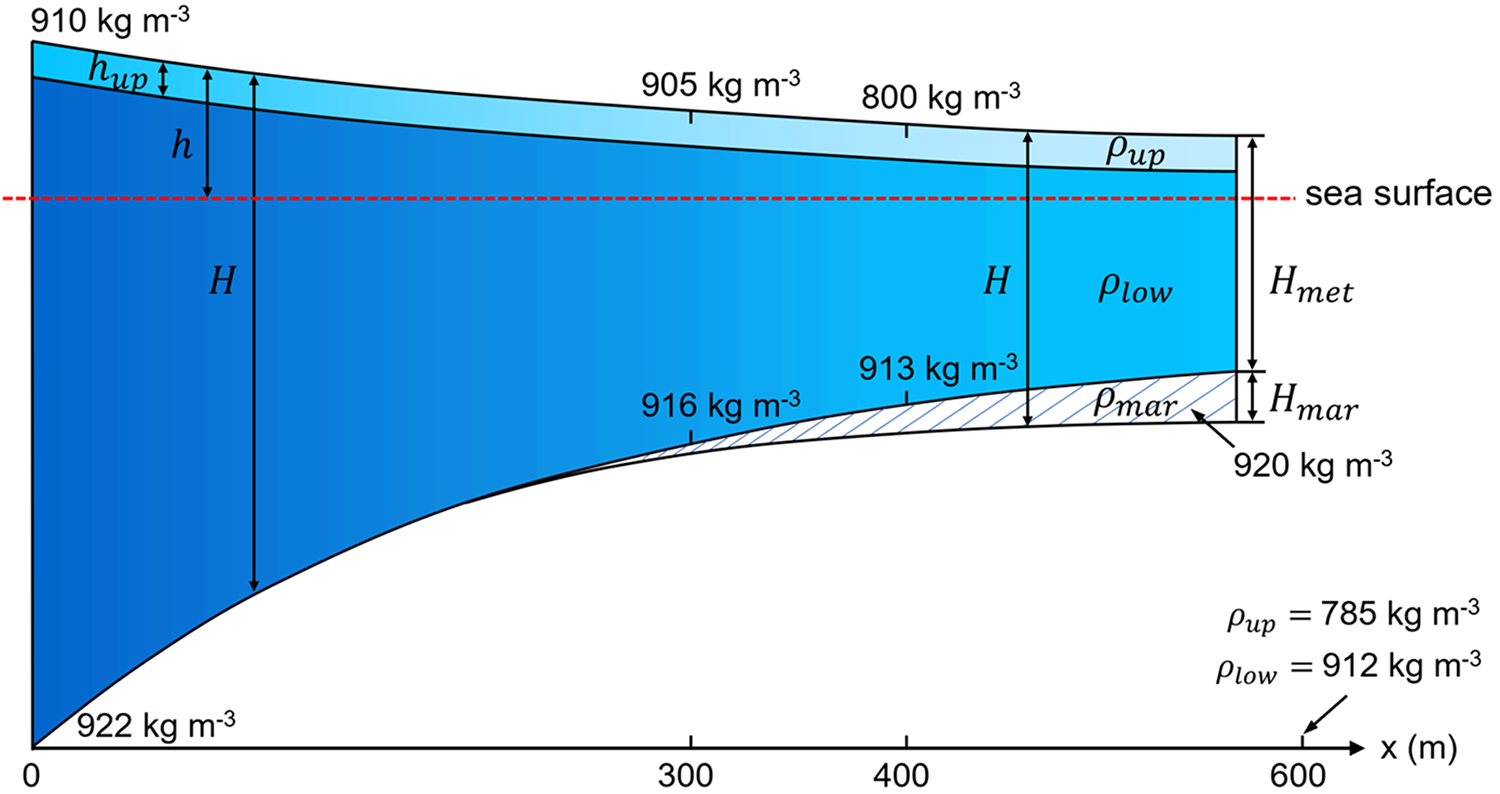
  ${H_{mar}}$ are the thicknesses of the meteoric and marine ice layers, respectively. As for the upper meteoric ice layer, we use the approach of Fricker and others (Reference Fricker, Popov, Allison and Young2001) to account for the effect of spatial differences in the snow accumulation regime and the temperature structure within the ice layers on column-average density. In this model, the meteoric ice layer is divided into two sub-layers with ${\rho _{up}}$ and ${\rho _{low}}$, respectively. In the horizontal direction, the density model divides the ice shelf into regions characterized by ablation and superimposed ice (between x = 0 and 300 m), a region in which the firn layer thickens downstream in a linear manner (x = 300–400 m), after which the firn layer reaches an equilibrium thickness. The thickness of the upper sub-layer, ${h_{up}}$, is 100 m (Fig. 1; Fricker and others, Reference Fricker, Popov, Allison and Young2001).
Diagram of a two-layer meteoric ice density model of the ice shelf with values changing linearly along the x-direction, with a third layer with a density of 920 kg m−3 in areas where marine ice exists. Labels show the ice density at different locations (0, 300, 400 and 600 m from the grounding line).
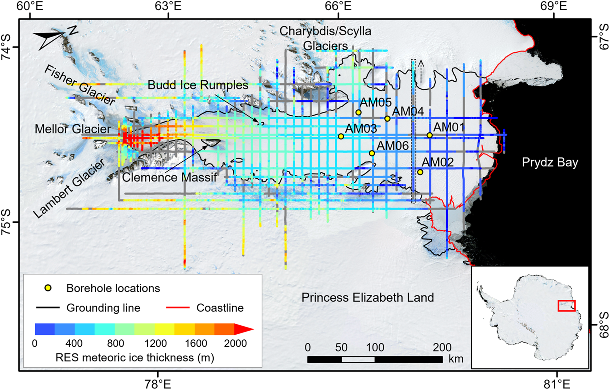
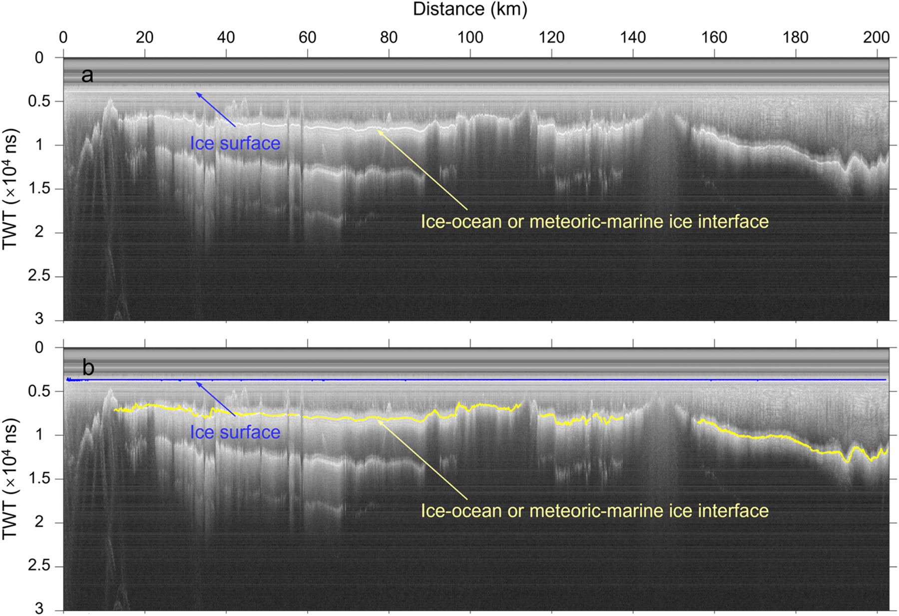
The thickness of the upper meteoric ice layer,  ${H_{met}}$, can be measured from RES data. The RES data were obtained from aerogeophysical surveys conducted between 2015 and 2019 using the fixed-wing airborne platform ‘Snow Eagle 601’ operated by the Polar Research Institute of China for the ICECAP project (Fig. 2). The onboard phase-coherent radar system operates at a central frequency of 60 MHz and a bandwidth of 15 MHz, functionally similar to the High Capability Airborne Radar Sounder (HiCARS) developed by the University of Texas Institute for Geophysics (Cui and others, Reference Cui2018, Reference Cui2020). Its low center frequency allows for deep ice penetration, while the relatively large bandwidth maintains sufficient resolution to detect key glaciological and geological features. Overall, this system achieves an along-track sampling interval of ∼20 m and a depth resolution of ∼10 m in air and ∼5.6 m in ice. The meteoric-marine ice interface (Moore and others, Reference Moore, Reid and Kipfstuhl1994) or ice–ocean interface (Fig. 3) was picked by Yang and others (Reference Yang2021) using a semiautomatic approach, which first manually bounded the range in which the interface should be found and used an algorithm to extract the brightest return from each trace (Blankenship and others, Reference Blankenship2017a,b; Cui and others, Reference Cui2020). The meteoric ice thickness was calculated by multiplying two-way travel time by the electromagnetic wave speed in ice (0.168 m ns−1; Cui and others, Reference Cui2018). No firn correction was applied; that is, the thickness includes firn and meteoric ice (Cui and others, Reference Cui2020). Meteoric ice-thickness data extracted in this way (Yang and others, Reference Yang2021) is used in the present work (Fig. 2).
Spatial distribution of meteoric ice thickness extracted from RES data from the ICECAP survey flights (Yang and others, Reference Yang2021) overlain on the Landsat Image Mosaic of Antarctica (LIMA; Bindschadler and others, Reference Bindschadler2008). The study area is indicated in the inset. The color bar represents meteoric ice thickness, ranging from 0 m (blue) to 2000 m (red), with missing values shown in gray. The yellow circles indicate the locations of six hot water boreholes in the AMISOR project. The black and red lines denote the grounding line and coastline, respectively, as provided by the dataset of Antarctic boundaries in Table 1 (Mouginot and others, Reference Mouginot, Scheuchl and Rignot2017). The dashed box indicates the RES data in Figure 3, and the arrow shows the flight direction.
(a) Example of RES data in the dashed box in Figure 2. (b) As (a) with picked interfaces, including the ice-shelf surface (blue line) and the interface of ice–ocean or meteoric-marine ice (yellow line). Between the surface and the bottom is meteoric ice.
However, in locations where basal freezing occurs, the RES data still typically show the bottom of the meteoric ice layer, owing to the high electromagnetic absorption in the marine ice layer (Thyssen, Reference Thyssen1988; Lambrecht and others, Reference Lambrecht, Sandhäger, Vaughan and Mayer2007), which is difficult to penetrate by radar. Thus, where marine ice may be present, there should be a difference between the calculated ice-shelf surface elevation  $h{^{\prime}}$ using ${H_{met}}$ and the measured surface elevation $h$, known as the hydrostatic height anomaly:
 \begin{equation}\delta h^{\prime} = h - h^{\prime}\end{equation}
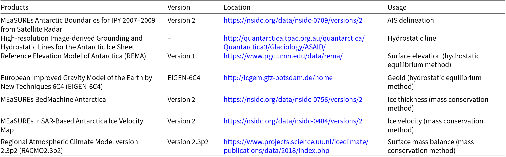
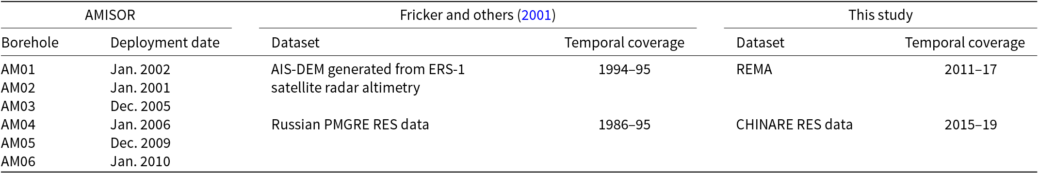
 Here,  $h$ is provided by the Reference Elevation Model of Antarctica (REMA; Howat and others, Reference Howat, Morin, Porter and Noh2018, Reference Howat, Porter, Smith, Noh and Morin2019). The elevations are from the 200 m-resolution REMA mosaic, acquired between 2011 and 2017 in our study area and are referenced to the mean sea level using the EIGEN-6C4 geoid (Förste and others, Reference Förste2014). The details of the datasets used here are listed in Table 1. $h{^{\prime}}$ is the surface elevation estimated using the meteoric ice thickness from the RES data when no marine ice is assumed to exist. We do not consider firn correction in the RES meteoric ice thickness (Cui and others, Reference Cui2020), which may introduce uncertainty in the thickness measurements. The potential errors resulting from this omission are discussed in Section 3.2. Instead, the column-averaged ice density model with two-layer meteoric ice takes a firn layer into account (Fricker and others, Reference Fricker, Popov, Allison and Young2001, Reference Fricker2002). Accordingly, we do not apply firn correction to the REMA freeboard when estimating the height anomaly.
Datasets used to calculate marine ice thickness
The hydrostatic height anomaly is used to identify areas where marine ice may be present. Then, assuming hydrostatic equilibrium and using the three-layer model, the thickness of marine ice can be estimated as
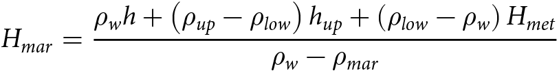 \begin{equation}{H_{mar}} = \frac{{{\rho _w}h + \left( {{\rho _{up}} - {\rho _{low}}} \right){h_{up}} + \left( {{\rho _{low}} - {\rho _w}} \right){H_{met}}}}{{{\rho _w} - {\rho _{mar}}}}\,\end{equation}
 in which $\,{\rho _{mar}}$ represents the column-averaged density of marine ice, and the other parameters are defined as above. The average density of seawater used in the calculation is 1029 kg m−3, as in Fricker and others (Reference Fricker, Popov, Allison and Young2001). The meteoric ice density is determined as shown in Fig. 1. For marine ice, we use a reference density of 920 kg m−3, which is slightly higher than that of pure ice due to the presence of brines and seawater (Craven and others, Reference Craven, Allison, Fricker and Warner2009). It should be noted that hydrostatic equilibrium may not be valid in the grounding zone of ice shelves (Griggs and Bamber, Reference Griggs and Bamber2011). Therefore, we masked the marine ice-thickness map using the hydrostatic line (Bindschadler and others, Reference Bindschadler2011a,Reference Bindschadler, Choi and Collaboratorsb), and only the results for the free-floating ice shelf are retained.
2.2. Mass conservation
Assuming that the ice shelf is incompressible and always in static equilibrium, the problem of mass conservation can be simplified to the continuity of ice volume (Jenkins and Doake, Reference Jenkins and Doake1991):
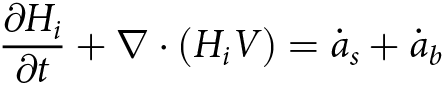 \begin{equation}\frac{{\partial {H_i}}}{{\partial t}} + \nabla \cdot \left( {{H_i}V} \right) = {\dot a_s} + {\dot a_b}\,\end{equation}
 in which  ${H_i}$ represents the equivalent thickness of solid ice, $V$ is the horizontal ice velocity, ${\dot a_s}$ is the net surface accumulation rate and ${\dot a_b}$ is the basal accumulation rate. In the context of a steady-state ice shelf, where $\partial {H_i}/\partial t = 0$, the horizontal divergence in volume flux is balanced by the sum of the surface and basal accumulation rates. Therefore, the basal accumulation rate, ${\dot a_b}$, can be obtained by
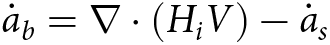 \begin{equation}{\dot a_b} = \nabla \cdot \left( {{H_i}V} \right) - {\dot a_s}\,\end{equation}
 In the case of floating ice, the shallow-shelf approximation indicates that velocity is constant at all depths and the velocity of meteoric and marine ice is uniform (Sanderson, Reference Sanderson1979). Expressing the horizontal ice velocity components along the x and y directions as  $u$ and $v$, respectively, Equation (6) becomes
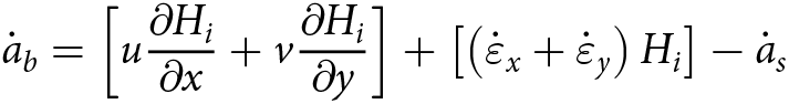 \begin{equation}{\dot a_b} = \left[ {u\frac{{\partial {H_i}}}{{\partial x}} + v\frac{{\partial {H_i}}}{{\partial y}}} \right] + \left[ {\left( {{{\dot \varepsilon }_x} + {{\dot \varepsilon }_y}} \right){H_i}} \right] - {\dot a_s}\,\end{equation}
 in which  ${\dot \varepsilon _x} = \partial u/\partial x$ and ${\dot \varepsilon _y} = \partial v/\partial y$ are the corresponding strain rates. To calculate ${\dot a_b}$, we employ two alternative datasets as the solid-ice equivalent thickness ${H_i}$: (1) the total thickness of the ice shelf from the hydrostatic equilibrium method (meteoric plus marine ice) with a firn correction applied to obtain ice–equivalent thickness, and (2) the ice-equivalent thickness layer from the BedMachine Antarctica, version 2 dataset (Morlighem, Reference Morlighem2020; Morlighem and others, Reference Morlighem2020), hereafter referred to as BMA. The BMA provides Antarctic ice thickness and estimation errors at a resolution of 500 m, with most of the ice-shelf area (including AIS) estimated from the early (1994–95) satellite radar altimeter data of the European Remote-sensing Satellite (ERS-1). The horizontal ice velocity data used here is from the MEaSUREs InSAR-based Antarctica Ice Velocity Map, version 2 dataset (Rignot and others, Reference Rignot, Mouginot and Scheuchl2017), which provides a digital mosaic of ice motion in Antarctica with a spatial resolution of 450 m derived from multiple satellite radar interferometry data between 1996 and 2016. Considering the random error of the data themselves, the ice thickness and velocity map are smoothed using a circular moving average filter with a 10 km radius before being used to calculate the ice-thickness gradient and strain rate to reduce the noise (Das and others, Reference Das2020). The net accumulation rate at the surface is based on the annual surface mass balance (SMB) data simulated by the regional atmospheric climate model version 2.3p2 (RACMO2.3p2; van Wessem and others, Reference van Wessem2018) at a spatial resolution of 27 km. For the calculation, the average SMB data from 1996 to 2016 is included as the net surface accumulation rate, given the coverage period of the ice velocity data.
We assume that there is no material conversion process at the interface between meteoric and marine ice, so the thickness of marine ice,  ${H_{mar}}$, can be derived from Equation (5) using mass conservation (Holland, Reference Holland2002):
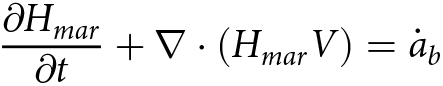 \begin{equation}\frac{{\partial {H_{mar}}}}{{\partial t}} + \nabla \cdot \left( {{H_{mar}}V} \right) = {\dot a_b}\,\end{equation}
 Aligning the x-axis with the flow line (Joughin and Vaughan, Reference Joughin and Vaughan2004), the change in  ${H_{mar}}$can be expressed as
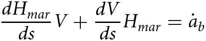 \begin{equation}\frac{{d{H_{mar}}}}{{ds}}V + \frac{{dV}}{{ds}}{H_{mar}} = {\dot a_b}\,\end{equation}
 in which  $s$ represents the distance along the flow line, which is positive along the ice flow. The marine ice thickness is estimated by combing Equations (7) and (9), starting from an initial position where ${H_{mar}} = 0$, which is the intersection of the flow line and the grounding line. We extract the flow lines based on the MEaSUREs InSAR-based ice velocity, calculate the marine ice thickness on each flow line and obtain a map of marine ice thickness through interpolation.
3. Results
3.1. Marine ice distribution
Our results show two longitudinally distributed marine ice accretion bands to the northwest of the AIS (Fig. 4a), mainly flanking the inflow of Charybdis and Scylla Glaciers, consistent with estimates from previous studies but thicker in some areas (Fricker and others, Reference Fricker, Popov, Allison and Young2001). In the east of the central ice shelf, located in the middle section of the profile A-A’, we find a thicker layer of marine ice than in previous studies, with a thickness of more than 30 m. In the south, where the ice shelf is relatively thick, we find smaller sites of local freezing distributed along-flow downstream from the grounding line and east of the Budd Ice Rumples. Fricker and others (Reference Fricker, Popov, Allison and Young2001) found a similar pattern of local freezing in this area. It is important to note, however, that the assumption of hydrostatic equilibrium is unlikely to be met everywhere in this region.
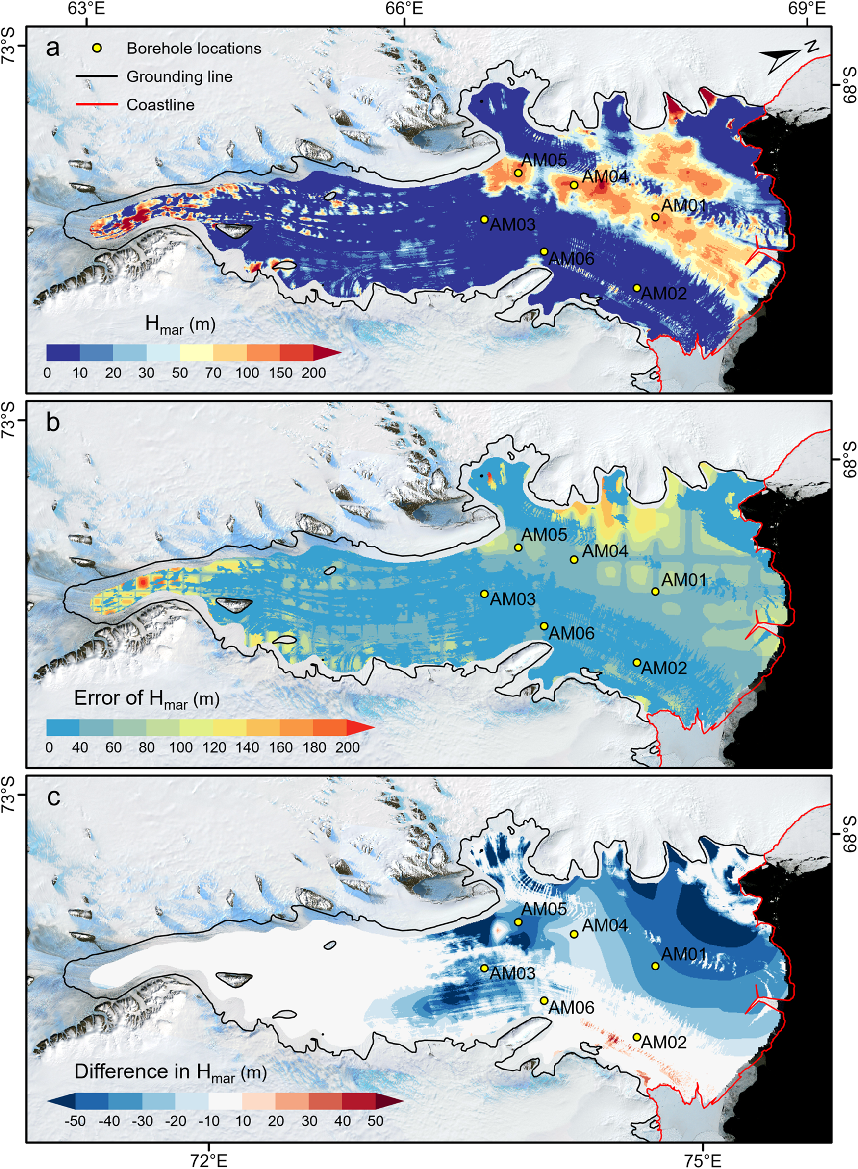
Marine ice distributions beneath the AIS derived from (a) the hydrostatic equilibrium method using RES ice thickness, (b) the mass conservation method using RES ice thickness and (c) the mass conservation method using BMA ice thickness. The yellow circles indicate the locations of six hot water boreholes in the AMISOR project. Purple lines represent the locations of the profiles plotted in Figure 6.

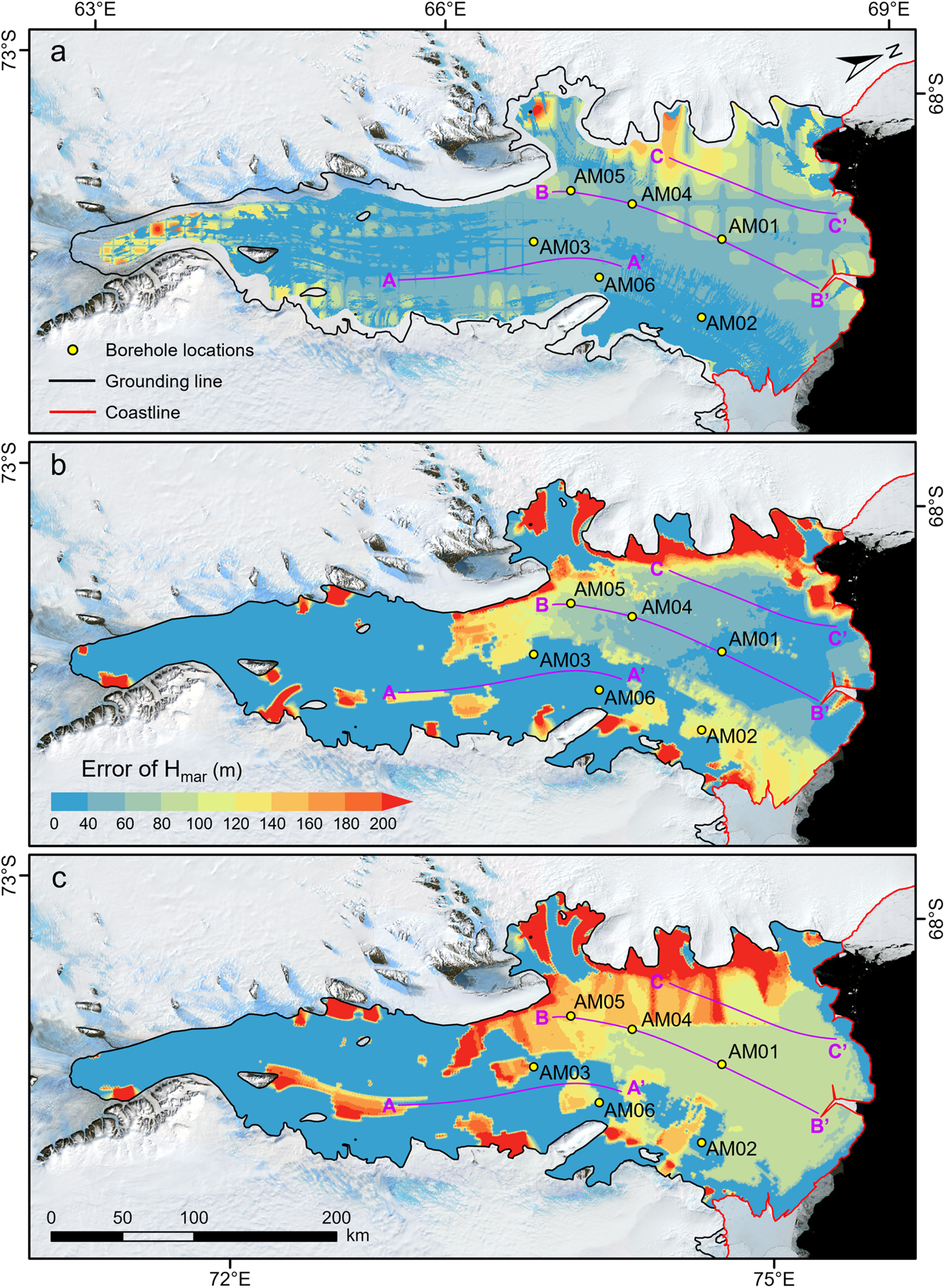
Error maps of marine ice thickness derived from (a) the hydrostatic equilibrium method using RES ice thickness, (b) the mass conservation method using RES ice thickness and (c) the mass conservation method using BMA ice thickness. The yellow circles indicate the locations of six hot water boreholes in the AMISOR project. Purple lines represent the locations of the profiles plotted in Figure 6.
The method of mass conservation yields an overall similar spatial pattern as the hydrostatic equilibrium method (Figs 4b and c), but there are some local differences. The mass conservation results using RES are generally thicker, and very high values are produced in the northwest of the two marine ice bands. Causes for differences among the three results are considered in Section 4.
3.2. Error estimation
Uncertainty in the estimated marine ice thickness is quantified by propagating errors associated with measured variables used in Equations (4) and (9). Errors in RES meteoric ice thickness mainly come from observation and the interpolation (Bamber and others, Reference Bamber2013; Chu and others, Reference Chu, Creyts and Bell2016). Observation errors depend on the precision in range estimates of the radar system and the uncertainty in the time-depth conversion, the latter including the uncertainty in the firn correction and the uncertainty in the electromagnetic wave speed in ice (Cavitte and others, Reference Cavitte2016; Winter and others, Reference Winter, Steinhage, Creyts, Kleiner and Eisen2019). Following Luo and others (Reference Luo2022), we use the precision of the range estimates of ±1.63 m for the HiCARS data. Although no firn correction is applied to the data we used, we provide an estimate of the errors caused by using a single electromagnetic wave speed in ice for the time-depth conversion based on the modeled firn air content (obtained from the BMA). Following Sugiyama and others (Reference Sugiyama, Enomoto, Fujita, Fukui, Nakazawa and Holmlund2010), taking an Antarctic snow dielectric permittivity of 1.644 (corresponding to a speed of 0.234 m ns−1), the estimate will be underestimated by 6 m at the ice front of the AIS where the firn is thickest (∼20 m), which is ∼3% of the ∼200 m ice thickness there. The electromagnetic wave speed in ice varies from 0.168 to 0.1695 m ns−1, which results in an increasing uncertainty with increased depth (or ice thickness; Fujita and others, Reference Fujita, Matsuoka, Ishida, Matsuoka and Mae2000; Luo and others, Reference Luo2022). In our study, the ice thickness of AIS increases from ∼200 m at the ice front to ∼2500 m at the southern grounding zone; thus, we consider a conservative representation of the uncertainty as ±22 m (within 1% of ice thickness). The uncertainty from the above factors is taken to be ±23 m.
Crossover analysis provides an alternative estimate of the error in the RES meteoric ice-thickness observations. We consider the differences in ice thickness between two measurements at the intersection of two flight lines within 20 m (approximately the along-track spatial sampling rate of the radar system). A total of 189 crossover differences are obtained within the ice shelf, with a standard deviation of ±37 m in ice thickness. This value only provides the consistency of the data, but we use it in subsequent calculations because it is the more conservative estimate of the error. The interpolation error in the RES meteoric ice thickness depends on the sampling interval of the observations and the variability of the measured ice thickness (Chu and others, Reference Chu, Creyts and Bell2016). Here, a geostatistical interpolation method, Empirical Bayesian kriging, is used to quantify the uncertainty of the interpolation results by calculating standard errors from a set of predictions generated from multiple semivariograms estimated at each location. We use the Geostatistical Analyst tools provided by ArcGIS to obtain the interpolated ice thickness map from the observed data and the corresponding interpolation error (https://doc.arcgis.com/). Combined with errors in the surface elevation that come from the REMA error (Howat and others, Reference Howat, Morin, Porter and Noh2018, Reference Howat, Porter, Smith, Noh and Morin2019), we produce a map of the uncertainty in the estimated marine ice thickness (Fig. 5a).
The densities of seawater, meteoric and marine ice are constants applied in our calculations. We use the same values for seawater and meteoric ice as in Fricker and others (Reference Fricker, Popov, Allison and Young2001). The value is slightly higher than the average seawater density directly observed through two of the AMISOR boreholes (1028 kg m−3; Craven and others, Reference Craven, Allison, Fricker and Warner2009). If this seawater density difference were widespread, it would lead us to slightly underestimate the marine ice thickness using the hydrostatic equilibrium method. A difference of 1 kg m−3 would result in an underestimation of <8 m in regions of marine ice in the northwest and central ice shelf. The meteoric ice density model may also be a source of bias. The presence of the firn at the surface is accounted for in the two-layer ice density model we used (Fricker and others, Reference Fricker, Popov, Allison and Young2001, Reference Fricker2002). The average meteoric ice density calculated by Craven and others (Reference Craven, Allison, Fricker and Warner2009) using two borehole measurements is within the range applied here following Fricker and others’s (Reference Fricker, Popov, Allison and Young2001) two-layer model. However, variations in the density of upper sub-layer meteoric ice (by 1 kg m−3) lead to a difference in the marine ice thickness estimate of <1 m, while variations in the value of the lower sub-layer lead to a difference of <8 m in areas of marine ice, including the northwestern and central regions of the ice shelf. A density of 920 kg m−3 is used for marine ice (Craven and others, Reference Craven, Allison, Fricker and Warner2009); however, we note that those authors observe spatial variation related to along-flow diagenesis of the accreted layer. Marine ice layer is expected to be denser where it is younger (and contains more brine), and the sense of the difference would again cause us to overestimate the marine ice thickness in some areas, with a pattern that is likely to be spatially structured. If the density of marine ice was underestimated by 1 kg m−3, the marine ice thickness will be overestimated by <2 m, with this effect occurring in >98% of areas where basal accretion is present. While these calculations provide a sense of scale for the possible error due to the selection of density values used in the calculation, each layer may have a different offset, either positive or negative. A worst case could be overestimates of meteoric ice density (upper and lower) plus underestimates of the densities of marine ice and seawater by 1 kg m−3, in which case the RMS is nearly 12 m. Additionally, changing the upper sub-layer meteoric ice thickness by 1 m will also result in about a 1 m change in the estimated marine ice thickness.
Uncertainty in the mass conservation method is due to errors in ice velocity, solid-ice equivalent thickness and surface accumulation rate. Here, we use the error map that accompanies the ice velocity data product (Rignot and others, Reference Rignot, Mouginot and Scheuchl2017) in our calculations. Errors in the solid-ice equivalent thickness are obtained from either the RES ice thickness error or the error estimate provided with the BMA (Morlighem, Reference Morlighem2020; Morlighem and others, Reference Morlighem2020). Errors in the surface accumulation rate are not reported for RACMO2.3p2 (van Wessem and others, Reference van Wessem2018); however, van Wessem and others’s (Reference van Wessem2018) elevation-dependent bias correction is applied.
The hydrostatic equilibrium method using RES data shows the smallest overall uncertainty in marine ice thickness estimation (Fig. 5), indicating its overall better performance compared to the other methods. The equilibrium-method error map is dominated by the uncertainty due to interpolation. Figure 5a shows that the large errors are on the northwest ice shelf (near the profile C-C’), where the interpolation from the sparsity of flight lines leads to larger uncertainty. In addition, the interpolation error is also relatively large near the grounding line, and we attribute this to the undulating terrain here. Uncertainty in the mass conservation method exhibits larger errors near the grounding line on the eastern and western sides of the ice shelf (Figs 5b and c), primarily arising from uncertainties in the basal accumulation rate. These uncertainties have a greater impact on error propagation because of the relatively small ice flow velocity gradients in these regions.
4. Discussion
4.1. Meteoric ice density model
In this study, the choice of meteoric ice density model plays a crucial role in estimating the marine ice thickness using the hydrostatic equilibrium method. We employ the meteoric ice density model from Fricker and others (Reference Fricker, Popov, Allison and Young2001) to enable effective comparison with their previous work and attempt change detection. This two-layer model represents meteoric ice as an upper and lower layer, each with different column-averaged densities, where the upper layer is set to 100 m thick and accounts for firn air content. While this model provides one way to characterize the meteoric ice density, it is not the only approach. An alternative method involves explicitly separating the firn layer, leading to a different ice density model for the hydrostatic equilibrium method, which we have also considered (Fig. A1 in Appendix A). In this alternative model, the meteoric ice column consists of an upper firn layer and a lower meteoric ice layer. The firn layer thickness is obtained from the BMA, while the lower meteoric ice density follows from Fricker and others (Reference Fricker, Popov, Allison and Young2001). The marine ice thickness estimated using this revised model also shows two longitudinally distributed bands in the northwest of the ice shelf, though the ice thickness is generally thinner than using the two-layer model (Fig. A1a). Additionally, patch basal accretion is observed downstream of the grounding line at the southern end of the ice shelf, whereas no significant accretion is detected east of the central ice shelf. The differences between the two model outputs clearly reveal the spatial pattern of firn layer thickness (Fig. A1c). These findings highlight that the choice of meteoric ice density model can have a dominant impact on hydrostatic equilibrium-based marine ice thickness estimation. It is also important to acknowledge that all meteoric ice density models inherently involve simplifications that influence the final estimates and must be considered when interpreting the results.
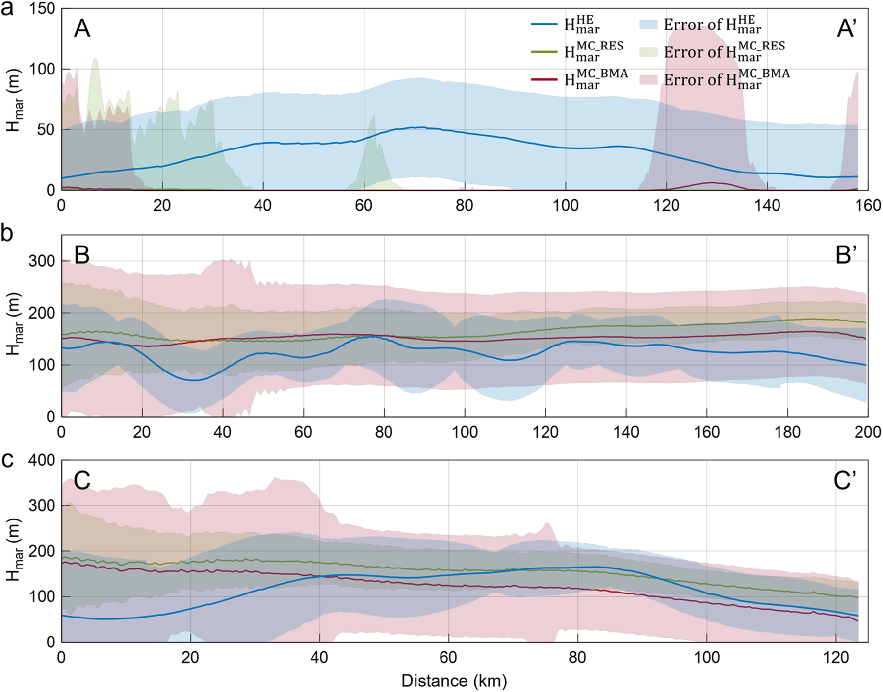
Plots of marine ice thickness and their errors by different methods along profiles (a) A-A’, (b) B-B’ and (c) C-C’ shown in Figures 4 and 5. The blue line shows the hydrostatic equilibrium results from RES data ( ${\text{H}}_{{\text{mar}}}^{{\text{HE}}}$), and the green and red lines represent the mass conservation results from RES ( ${\text{H}}_{{\text{mar}}}^{{\text{MC\_RES}}}$) and BMA data ( ${\text{H}}_{{\text{mar}}}^{{\text{MC\_BMA}}}$), respectively. The shadings of corresponding colors indicate error ranges. Note that the thickness estimated by the hydrostatic equilibrium method has been smoothed using a circular moving average filter with a 10 km radius to remove noise associated with crevasses and facilitate comparison.
4.2. Comparison of marine ice-thickness estimates
While the three results are in broad agreement regarding the spatial pattern of marine ice accumulation on the base of the ice shelf, differences emerge. Three profiles in marine ice accumulation regions show that the differences between the mass conservation and hydrostatic equilibrium estimates generally fall within the uncertainty range of the hydrostatic equilibrium method (Fig. 6). The glaciological contexts and limitations in the observational data explain why some differences emerge. First, the results are in qualitative agreement where velocity gradients are relatively large (profiles B-B’ and C-C’ in Fig. 6), while they disagree where velocity gradients are smaller (profile A-A’ in Fig. 6). The horizontal smoothing inherent in spatial data products appears to reduce the sensitivity of the mass-conservation method. Alley and others (Reference Alley, Scambos, Anderson, Rajaram, Pope and Haran2018) discuss length-scale challenges in their careful analysis of strain-rate estimations. The hydrostatic equilibrium and mass conservation methods also disagree where ice-thickness gradients are large, for example, downstream of the grounding line. Differences along the profile B-B’ near 32 km and at the beginning of the profile C-C’ are likely due to data gaps, which required interpolation over long distances in some areas. Moreover, the assumption of steady state required by the mass conservation method may not be correct, and if not, further complications may arise due to the somewhat different observational epochs represented by different data products. Nevertheless, given the associated uncertainties, the estimated marine ice thicknesses agree reasonably well in most areas of the ice shelf, with differences generally within 50 m (Fig. A2 in Appendix A).
4.3. Comparison with other results
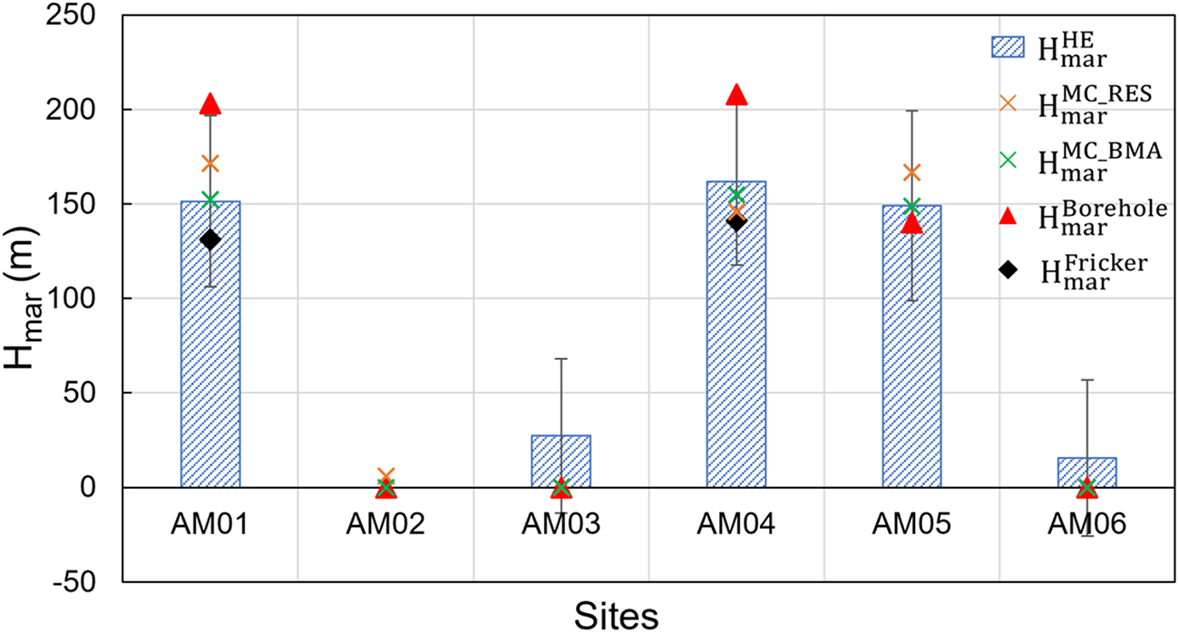
Marine ice thickness was observed directly or inferred from other measurements by the AMISOR project at six hot water borehole sites (Fig. 7; Allison and Craven, Reference Allison and Craven2000; Craven and others, Reference Craven, Warner, Galton-Fenzi, Herraiz-Borreguero, Vogel and Allison2014). Both the hydrostatic equilibrium and mass conservation methods yield thinner marine ice than observed at AM01 and AM04 and slightly thicker marine ice than the ‘>140 m’ reported for AM05, which was obtained using fiber-optic temperature (Craven and others, Reference Craven, Warner, Galton-Fenzi, Herraiz-Borreguero, Vogel and Allison2014). Both our RES-based hydrostatic result and Fricker and others’s (Reference Fricker, Popov, Allison and Young2001) earlier result using the same method indicate thin marine ice layers AM03 and AM06, where no marine ice was observed at the borehole sites. These differences reflect the challenge in comparing point values with maps of fields characterized by large spatial variability as well as uncertainty in the remote-sensing based approaches. Because the various observations were made using data collected over different time intervals (Table 2), the differences may also reflect changes over time in the ice shelf.
Estimated marine ice thickness of the hydrostatic equilibrium method ( ${\text{H}}_{{\text{mar}}}^{{\text{HE}}}$) with error bars, the estimated results of the mass conservation method ( ${\text{H}}_{{\text{mar}}}^{{\text{MC\_RES}}}$ and ${\text{H}}_{{\text{mar}}}^{{\text{MC\_BMA}}}$), the estimates by Fricker and others (Reference Fricker, Popov, Allison and Young2001) ( ${\text{H}}_{{\text{mar}}}^{{\text{Fricker}}}$; Craven and others, Reference Craven, Allison, Fricker and Warner2009), and the measurements at boreholes ( ${\text{H}}_{{\text{mar}}}^{{\text{Borehole}}}$). Error bars are larger for the mass conservation calculations. Note that the marine ice thickness was not directly measured at AM05, but later inferred to be >140 m from fiber-optic temperature data (Craven and others, Reference Craven, Warner, Galton-Fenzi, Herraiz-Borreguero, Vogel and Allison2014).
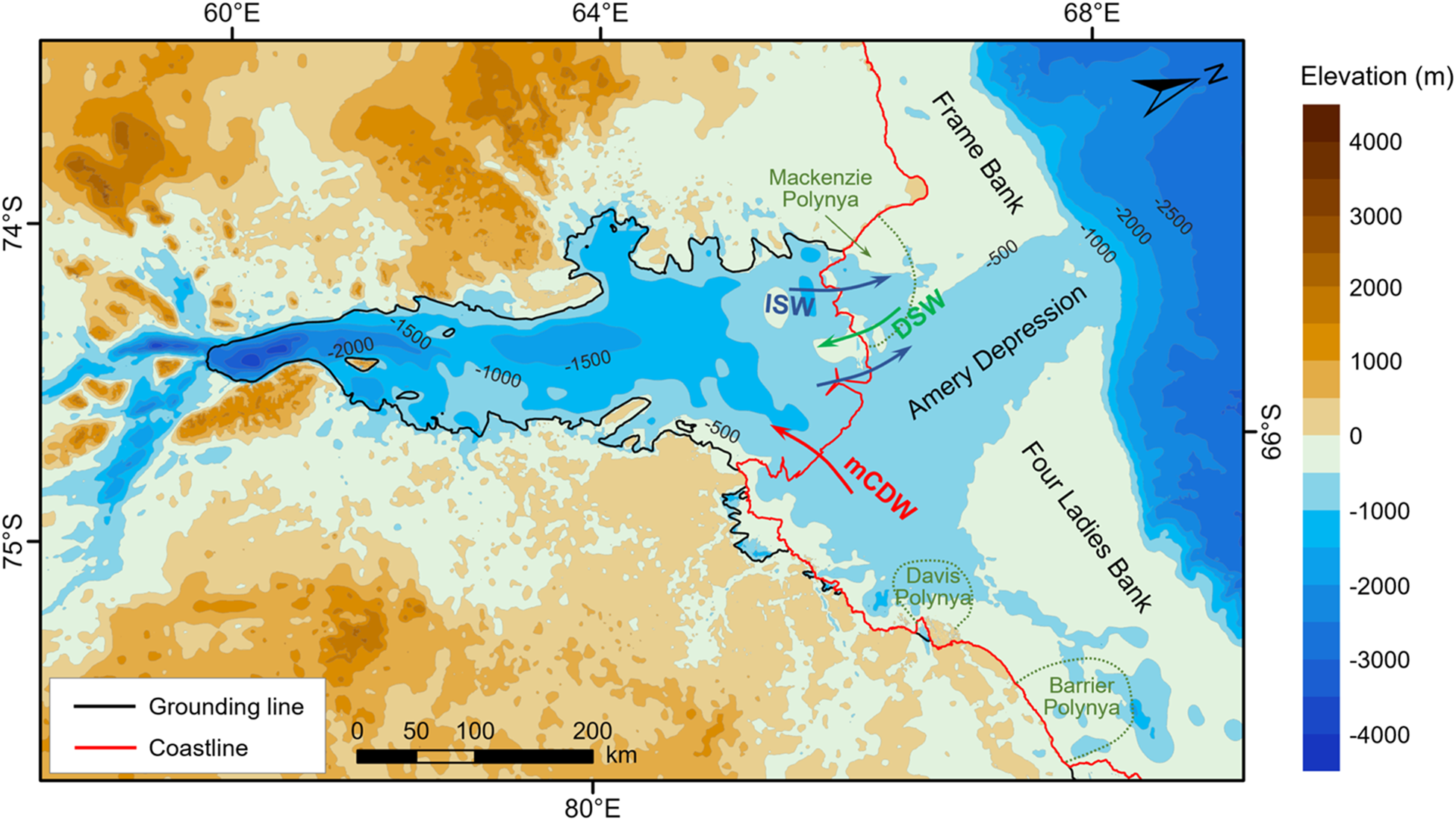
Seafloor topography/bathymetry from Yang and others (Reference Yang2021) beneath the AIS and bed elevation from the Bedmachine Antarctica dataset (outside the AIS). Red and green arrows represent the inflow of mCDW and DSW, respectively, while the blue arrow depicts the outflow of ISW.
Deployment dates of boreholes in the AMISOR project (Craven and others, Reference Craven, Warner, Galton-Fenzi, Herraiz-Borreguero, Vogel and Allison2014) and temporal coverage of the datasets used in earlier studies (Fricker and others, Reference Fricker, Popov, Allison and Young2001) and this study
Our new RES-based map of marine ice thickness using the hydrostatic method is broadly similar to the earlier map made using similar data and the same method (Fricker and others, Reference Fricker, Popov, Allison and Young2001), but differences emerge. First, we find an overall thicker marine ice layer near the calving front, on the order of a few tens of meters. Moving upstream along the flowband containing AM01 to AM05, our estimated ice thickness is similar to the early 1990s estimate in the area around AM01, but we find thicker marine ice upstream from there. Similarly, we find a thicker marine ice layer at and upstream of AM03 and AM06, on the order of a few tens of meters. We also find more widespread marine ice accumulation downstream of the grounding zone than reported by Fricker and others (Reference Fricker, Popov, Allison and Young2001).
4.4. Formation of marine ice
Marine ice thicknesses calculated in this study are generally thicker than estimates made using data spanning the years from 1986 to 1995 (Fricker and others, Reference Fricker, Popov, Allison and Young2001) and generally closer to thicknesses observed via boreholes between 1999 and 2010. It is possible that the differences between our new results and the older observations represent an increase in basal freezing over time, due to either variability or change in the ice–ocean system. The oceanographic processes in Prydz Bay (Fig. 8) play a crucial role in the formation of marine ice, which is primarily driven by two water masses: Dense Shelf Water (DSW), which forms in coastal polynyas and sinks into the cavity under the western flank of the ice shelf, and modified Circumpolar Deep Water (mCDW) inflow on the eastern flank (Herraiz-Borreguero and others, Reference Herraiz-Borreguero, Coleman, Allison, Rintoul, Craven and Williams2015, Reference Herraiz-Borreguero2016). The two inflowing water masses produce two distinct types of Ice Shelf Water (ISW), with ISW formed from DSW observed to flow out from the AIS cavity along the western flank, where marine ice is observed to form (Fricker and others, Reference Fricker, Popov, Allison and Young2001; Herraiz-Borreguero and others, Reference Herraiz-Borreguero, Coleman, Allison, Rintoul, Craven and Williams2015; Wang and others, Reference Wang2023).
Time series observations from the AMISOR project show that seasonal DSW intrusion under the ice shelf changes the water column stratification by tilting isopycnal surfaces, raising ISW toward the shelf base and forming frazil ice (Herraiz-Borreguero and others, Reference Herraiz‐Borreguero, Allison, Craven, Nicholls and Rosenberg2013). Given that marine ice formation is closely linked to ISW supply, either a change in ISW production rate or a change in the timing or intensity of DSW intrusion under the AIS could account for an increase in the amount of marine ice. This, in turn, could be due to variability in polynya activity and DSW production on the shelf (Tamura and others, Reference Tamura, Ohshima, Fraser and Williams2016; Gu, Reference Gu2024). Additionally, the Prydz Bay Gyre and the Eastern Coastal Current transport mCDW from the eastern side of AIS to the shelf bottom (Smith and others, Reference Smith, Zhaoqian, Kerry and Wright1984; Wong and others, Reference Wong, Bindoff and Forbes1998; Liu and others, Reference Liu, Wang, Cheng, Xia, Li and Xie2017). Variability or change in mCDW circulation under the shelf could also be a source of increased ISW, and in turn, more marine ice formation.
Both the present study and the earlier estimates of Fricker and others (Reference Fricker, Popov, Allison and Young2001) predict the patchy occurrence of marine ice downstream of the AIS grounding line, east of the Budd Ice Rumples, and south of the Clemence Massif. Altimetry-derived estimates of basal melt rates in Adusumilli and others (Reference Adusumilli, Fricker, Medley, Padman and Siegfried2020) identify localized freezing near the grounding line, in line with our results, though in a more restricted area than we find. Ocean models (Galton-Fenzi and others, Reference Galton-Fenzi, Hunter, Coleman, Marsland and Warner2012) predict freezing east of the ice rumples but strong melting elsewhere in this region. The apparent contradiction may be explained if some of the cold meltwater formed in this area was rising and refreezing in basal crevasses. Refreezing in basal crevasses downstream of the grounding line was also recently observed downstream of the Kamb Ice Stream grounding line (Lawrence and others, Reference Lawrence2023). It is worth noting that the assumption of hydrostatic equilibrium may not always hold near the grounding line, and for this reason, we excluded ice between the grounding line and the hydrostatic line (Bindschadler and others, Reference Bindschadler2011a,Reference Bindschadler, Choi and Collaboratorsb) in our calculations. The propagated errors are relatively high close to the grounding line (Fig. 5a), nevertheless, even when accounting for these uncertainties in the estimated marine ice-thickness map, the localized refreezing downstream of the grounding line remains non-negligible.
5. Conclusions
Marine ice contributes to the stability of Antarctic ice shelves. In this study, we have provided a new estimate of the spatial distribution and thickness of marine ice underneath the AIS using meteoric ice thickness extracted from RES data collected during the CHINARE seasons (2015–19) for the ICECAP project. Our results show the distribution of two longitudinal marine ice accretion bands in the northwest of AIS, which we conclude to have thickened between our observations and the earlier RES observation campaign. Changes in DSW production on the continental shelf associated with polynya variability are the likely source of such change. We also report accretions of marine ice in the central ice shelf and downstream of the grounding line, areas that have not been a focus of past studies. Our analysis also demonstrates the large errors associated with remote estimation of marine ice thickness and points to the need for more extensive in situ measurements of ice shelves to more accurately assess the ice-shelf structure and monitor interaction processes between the ice shelf and the ocean. Furthermore, the impact of ice accretion at the bottom on ice dynamics and stability of ice shelves remains to be investigated. Overall, this study contributes to a better understanding of ice–ocean interaction and the stability of Antarctic ice shelves.
Data availability statement
The meteoric ice thickness used in this study and the estimated marine ice thickness and error data are available at https://doi.org/10.5281/zenodo.15226103. The Reference Elevation Model of Antarctica (REMA) is available at the US Polar Geospatial Center (PGC; https://www.pgc.umn.edu/data/rema/); the EIGEN-6C4 is available at the GFZ German Research Centre for Geosciences (http://icgem.gfz-potsdam.de/home); the MEaSUREs Antarctic Boundaries for IPY 2007–2009 from Satellite Radar, Version 2 (https://doi.org/10.5067/AXE4121732AD), MEaSUREs BedMachine Antarctica, Version 2 (https://nsidc.org/data/nsidc-0756/versions/2), and MEaSUREs InSAR-Based Antarctica Ice Velocity Map, Version 2 (https://nsidc.org/data/nsidc-0484/versions/2) are available at the National Snow & Ice Data Center (NSIDC); the regional atmospheric climate model version 2.3p2 (RACMO2.3p2) is available from van Wessem and others (2018; https://www.projects.science.uu.nl/iceclimate/publications/data/2018/index.php); the hot-water-drilled borehole data are available at the Australian Antarctic Data Centre (https://data.aad.gov.au/metadata/records/ASAC_1164); and the seafloor topography beneath the Amery Ice Shelf, East Antarctica, is available from Yang and others (2021; http://doi.org/10.5281/zenodo.5651609).
Acknowledgements
This work is supported in part by the National Natural Science Foundation of China under Grant 42276257, 41941006, and 41876230. The Australian Antarctic Division provides funding and logistical support through projects AAS 4346 and 4511. J.S.G. acknowledges support from US National Science Foundation grants OPP-2114454 and PLR-1543452; D.D.B., J.S.G., F.A.H., and D.A.Y. acknowledge support from the G. Unger Vetlesen Foundation, the Department for Business Energy and Industrial Strategy, the British Council, and the US State Department. We would like to thank the Chinese National Antarctic Research Expedition (CHINARE) and University of Texas Institute for Geophysics (UTIG) for their help in the field RES data collection. We are grateful to the editor and reviewers for their time in improving this manuscript.
Competing interests
There are no competing interests.
Appendix A
(a) Marine ice thickness beneath the AIS derived from the hydrostatic equilibrium method using RES ice thickness when firn layer is taken into account in the meteoric ice density model. (b) Error map of (a). (c) Difference in marine ice thickness derived from the meteoric ice density model considering firn layer compared to the two-layer model. The yellow circles indicate the locations of six hot water boreholes in the AMISOR project.
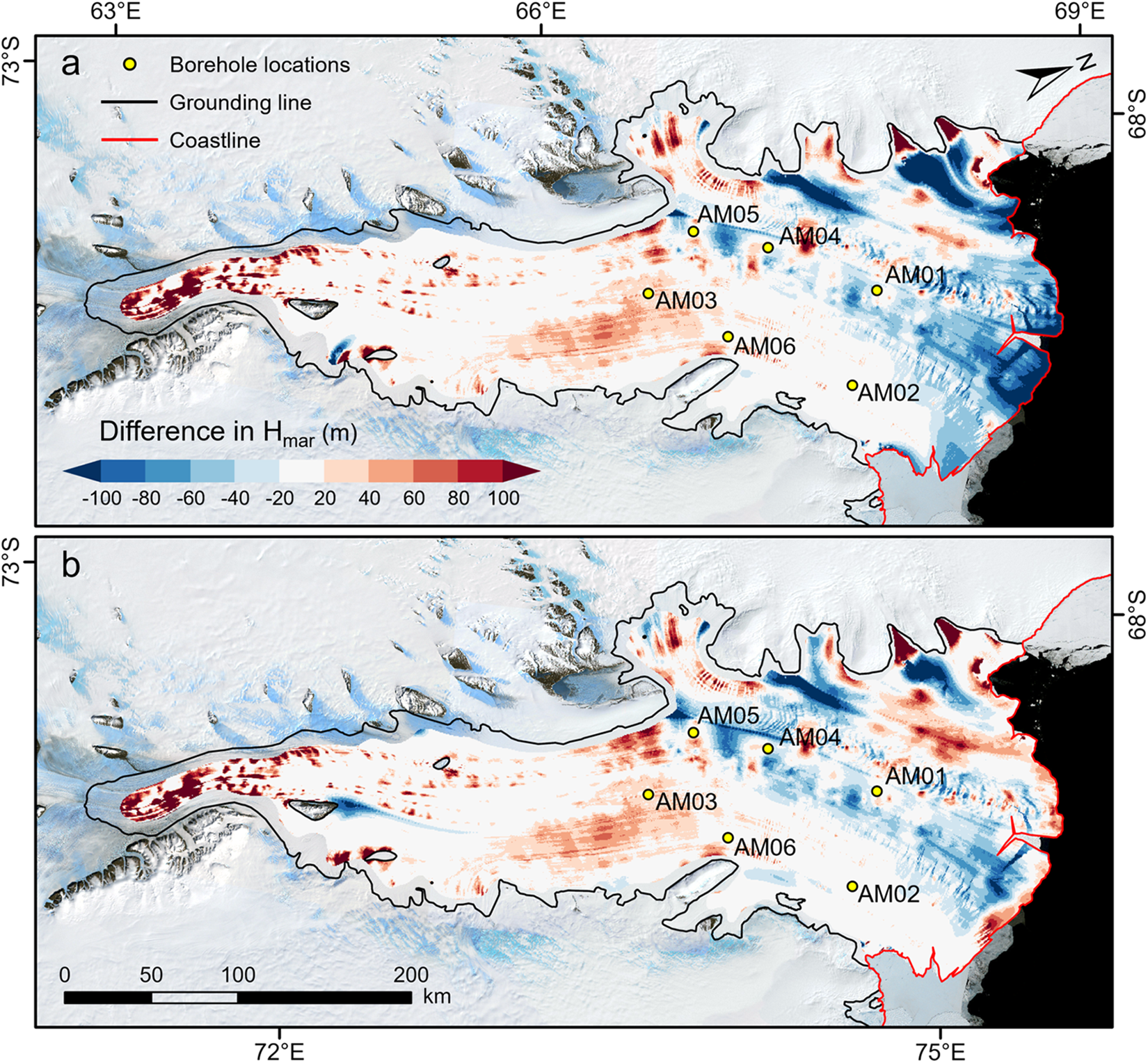
Difference in marine ice thickness derived from the mass conservation method using (a) RES ice thickness and (b) BMA ice thickness compared to the hydrostatic equilibrium method using RES ice thickness. The yellow circles indicate the locations of six hot water boreholes in the AMISOR project.


 Open access