1 INTRODUCTION
The search for high-redshift objects has rapidly developed in the last decades as astronomers attempt to understand the evolution of galaxies throughout the history of the Universe, with the current frontier being at redshift z ~ 10, or ~13.4 Gyr lookback time (Oesch et al. Reference Oesch2016; Zitrin et al. Reference Zitrin2014; Coe et al. Reference Coe2013). Since the large majority of these distant sources are very faint (m AB ~ 26 for a typical L * galaxy at z ~ 6), deep images of the sky are needed. The Hubble Space Telescope (HST) has carried out a number of surveys that had the detection of high-redshift galaxies as a key science motivation, starting from the pioneering Hubble Deep Field survey (HDF; Williams et al. Reference Williams1996a), and then continuing to improve depth and area covered thanks to technological progress offering newer instrumentation, with the Hubble Ultra Deep Field survey (HUDF; Beckwith et al. Reference Beckwith2006), the Great Observatories Origins Deep Survey (GOODS; Giavalisco et al. Reference Giavalisco2004), the Cosmic Assembly Near-infrared Deep Extragalactic Legacy Survey (CANDELS; Koekemoer et al. Reference Koekemoer2011), the HST Frontier Fields (Lotz et al. Reference Lotz2017), and the Brightest of Reionizing Galaxies Survey (BoRG; Trenti et al. Reference Trenti2011), among others.
The most common techniques used to identify high-redshift galaxies from broadband imaging are the Lyman-break method (Steidel et al. Reference Steidel, Giavalisco, Dickinson and Adelberger1996), which has been widely applied to the highest redshift (z ≳ 4) samples (e.g. Bouwens et al. Reference Bouwens2015), and other photometric redshift selection methods (e.g. Coe et al. Reference Coe, Benítez, Sánchez, Jee, Bouwens and Ford2006). Due to the ubiquitous presence of hydrogen, which has a large ionisation cross-section, photons with λ < 912 Å are heavily absorbed by neutral hydrogen in its ground state, and only have a low probability of escaping from a galaxy without being absorbed. Hydrogen in the intergalactic medium also contributes to the Lyman-break, effectively absorbing a large fraction of photons emitted by a high-redshift source at λ < 1216 Å for sources at z ≳ 4. Although generally highly effective, the Lyman-break method has some limitations as it may preferentially select only certain subsets of the galaxy population at high-z, such as relatively unobscured, actively star-forming galaxies (e.g. see Stanway, Bremer, & Lehnert Reference Stanway, Bremer and Lehnert2008). Recent examples of the application of this technique include Calvi et al. (Reference Calvi2016), Bouwens et al. (Reference Bouwens2016), and Hathi et al. (Reference Hathi2010). The Lyman-break selection is a special case of multicolour photometric selection, which is most effective when a spectral break is present in the sources targeted by the survey. However, spectra of galaxies can have other characteristic features in addition to the Lyman-break, which can be observed in different wavelengths and can improve the candidates selection. For instance, infrared data can be used to detect the Balmer break in z ≳ 5 galaxies (Mobasher et al. Reference Mobasher2005), and photometric redshift accuracy and reliability improves when there is a large number of bands available.
Arguably, one of the most fundamental observables from high-redshift surveys is the measurement of the galaxy luminosity function (LF). Generally, studies of the LF at cosmological distances are carried out with galaxy candidates from photometric catalogues (either using photometric redshift estimations or a dropout technique) as spectroscopic samples are significantly more challenging to construct and thus limited in numbers. Even after accounting for the most recent advancements in the field, that yielded catalogues of photometric sources at z ≳ 4 including more than 10000 sources (Bouwens et al. Reference Bouwens2015), the LF shape is still debated, and the topic is a very active research area (e.g. Ishigaki et al. Reference Ishigaki, Kawamata, Ouchi, Oguri and Shimasaku2017; Bouwens et al. Reference Bouwens2015; Atek et al. Reference Atek2015; Bowler et al. Reference Bowler2014; Bradley et al. Reference Bradley2012). To go from counting galaxies to the construction of the LF, it is imperative to understand completeness and efficiency, i.e. what fraction of all the existing galaxies with a given spectral energy distribution, morphological properties, and redshift range is identified in an observed sample. Accordingly, a machinery able to estimate the recovery fraction is critically needed for robust LF estimations. Yet, despite the large number of high-redshift galaxy surveys carried out in the last 20 yrs since the original HDF (Williams et al. Reference Williams1996b), there is not a unified publicly available tool to estimate their completeness and source recovery. Such a software tool is not only important for the estimation of volume and LFs, but also to investigate the properties of the galaxies a survey fails to detect, and reasons for missing them.
The classic approach to completeness estimates is to insert simulated galaxies in the observed images and quantify the recovery efficiency. There are two main methods typically used to create these simulated sources. One is based on starting from images of galaxies acquired in similar observations (for example, at lower redshift), that are modified/rescaled to fit the desired properties of the sample to simulate. The other one is the creation of artificial light profiles from theoretical models of the expected surface brightness profiles. Examples of LF studies utilising the former approach are Bershady, Lowenthal, & Koo (Reference Bershady, Lowenthal and Koo1998), Imai et al. (Reference Imai, Matsuhara, Oyabu, Wada, Takagi, Fujishiro, Hanami and Pearson2007), and Cristóbal-Hornillos et al. (Reference Cristóbal-Hornillos2009). The latter approach is applied in Bowler et al. (Reference Bowler2015), Oesch et al. (Reference Oesch2014), Jiang et al. (Reference Jiang2011), among others. This is also the approach taken in this paper, primarily because of its flexibility in the definition of shape, size, and the spectral energy distribution of the artificial sources, which make it well suited for a broader range of applications.
This paper presents a python-based tool to estimate the completeness of galaxy surveys, the GaLAxy survey Completeness AlgoRithm (GLACiAR hereafter). The software produces a photometric output catalogue of the simulated sources as main output, and associated higher level products to easily quantify source completeness and recovery. In particular, two main analyses are automatically performed: the first is the calculation of the fraction of sources recovered as a function of magnitude in the detection band (i.e. the survey completeness); and the second one is a more comprehensive characterisation of the recovery efficiency taking into account all survey bands allowing the user to implement multicolour selection criteria to identify high-redshift galaxies (i.e. the survey source selection efficiency as a function of both input magnitude and redshift).
The current version of the software is limited to handle blank (non-lensed) fields, but the code structure has been designed with the idea of introducing, in a future release, the capability to load a user-defined lensing magnification map and add artificial objects in the source plane. This would allow natural application of the code to quantify completeness for lensing surveys, which is a powerful complementary method to find high-redshift galaxies as we can observe intrinsically faint galaxies that are magnified by foreground objects. Surveys such as the Cluster Lensing And Supernova survey with Hubble (CLASH; Postman et al. Reference Postman2012) and the Herschel Lensing Survey (HLS; Egami et al. Reference Egami2010) are some examples.
This paper is organised as follows: Section 2 discusses the principles of the code, with our specific algorithmic implementation presented in Section 3. Section 4 illustrates the application of the code to part of the BoRG survey and compares the results obtained to previous determinations of the survey completeness and selection functions. Finally, we summarise and conclude in Section 5.
2 GENERAL OVERVIEW
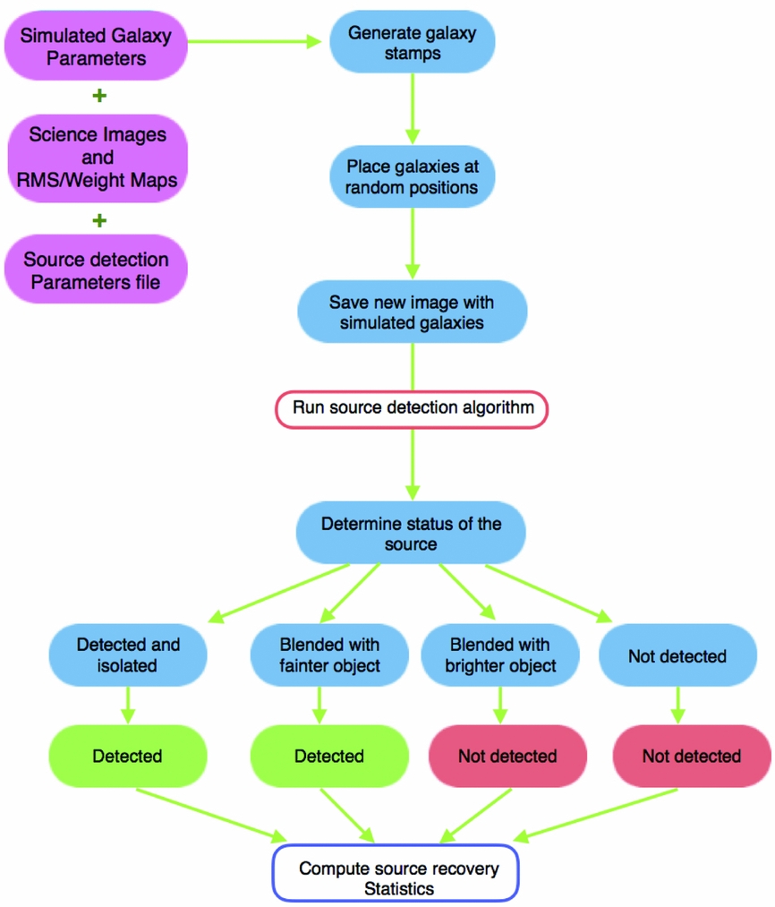
GLACiAR is structured modularly for maximum efficiency and flexibility. First, it creates artificial galaxies and adds them to the observed science images. Then, a module to identify sources is called, which builds catalogues with photometric information of the detected objects. The output catalogues from the original science images are compared with the ones from the new frames in order to identify the artificial sources recovery and multiband photometric information. Finally, another module is available to automatically calculate their recovered fraction as a function of input magnitude and simulated redshift. Figure 1 provides a high-level summary of the algorithm.
Logic diagram of GLACiAR’s code structure. User-defined parameters and a science image (with its associated RMS map) are taken as input, with the code then generating simulated galaxy stamps, which are added to the science image at random positions, sampled from a uniform distribution. A detection algorithm is run on these images, and its output is used to determine statistics on source recovery.
To identify sources, we limit ourselves to the use of SExtractor (Bertin & Arnouts Reference Bertin and Arnouts1996) for the current release, but we expect to expand the functionality of GLACiAR to allow the use of photutils (Bradley et al. Reference Bradley2016) in future versions.
A set of galaxy stamps are generated with sources that follow a Sérsic luminosity distribution (Sérsic Reference Sérsic1968) with parameters defined by the user. These artificial galaxies are placed at random positions on the images of the survey. In order to run the code, a parameters file (described in Section 3.1) must be completed by the user to define the features of the simulated galaxies, such as magnitude, size, redshift, among others. Along with this, GLACiAR requires other files: the science images, a list with the names of the fields (for one or more than one), the SExtractor parameters, frames with noise intensity maps (RMS or weight maps, depending on which ones are used to run the source identification), and the point spread functions (PSFs) in the filter(s) used to acquire the image(s). These inputs are described in more detail in Section 3.2.
2.1. Sérsic profiles for artificial galaxies
For the characterisation of the artificial galaxy’s surface brightness, we use the Sérsic luminosity profile (Sérsic Reference Sérsic1968) which has been widely shown to be a good fit for different types of galaxies given its flexibility (e.g. Peng et al. Reference Peng, Ho, Impey and Rix2002; Graham & Driver Reference Graham and Driver2005; Häußler et al. Reference Häußler2013). This profile is defined as
 $$\begin{equation}
I(R) = I_{e}\text{exp}\left\lbrace -b_{n}\bigg [\bigg (\frac{R}{R_e}\bigg )^{\frac{1}{n}}-1\bigg ]\right\rbrace,
\end{equation}$$
$$\begin{equation}
I(R) = I_{e}\text{exp}\left\lbrace -b_{n}\bigg [\bigg (\frac{R}{R_e}\bigg )^{\frac{1}{n}}-1\bigg ]\right\rbrace,
\end{equation}$$
with I e being the intensity at the radius that encloses half of the total light, R e; n is the Sérsic index, which describes the shape of the profile; and b n is a constant defined in terms of this index, which follows from our choice to normalise the profile with I e.
To obtain the luminosity of a galaxy within a certain radius, we follow the approach by Graham & Driver (Reference Graham and Driver2005) integrating equation (1) over a projected area A = πR 2, ending up with
 $$\begin{equation}
L(<R) = I_{e}R_{e}^{2}2\pi n\frac{e^{b_{n}}}{(b_{n})^{2n}}\gamma (2n,x),
\end{equation}$$
$$\begin{equation}
L(<R) = I_{e}R_{e}^{2}2\pi n\frac{e^{b_{n}}}{(b_{n})^{2n}}\gamma (2n,x),
\end{equation}$$
where γ(2n, x) is the incomplete gamma function, and
 $$\begin{equation}
x = b_{n} \bigg (\frac{R}{R_{e}}\bigg )^{\frac{1}{n}}.
\end{equation}$$
$$\begin{equation}
x = b_{n} \bigg (\frac{R}{R_{e}}\bigg )^{\frac{1}{n}}.
\end{equation}$$
To calculate b n, we follow Ciotti (Reference Ciotti1991), and taking the total luminosity, we obtain
 $$\begin{equation}
\Gamma (2n) = 2\gamma (2n,b_{n}),
\end{equation}$$
$$\begin{equation}
\Gamma (2n) = 2\gamma (2n,b_{n}),
\end{equation}$$
where Γ is the complete gamma function. From here, the value of b n can be obtained.
2.2. Artificial galaxy data
We create the stamp of an artificial galaxy according to a set of input (user-specified) parameters, which describe the free parameters of the Sérsic profile described in equation (2). n is the Sérsic index and it can be defined arbitrarily in GLACiAR. For the effective radius R e, the input is the proper size in kiloparsecs at a redshift z = 6, which is converted into arcseconds and scaled by the redshift with (1 + z)−1. The default value is R e = 1.075 kpc, chosen according to previous completeness simulations for the BoRG survey (Bradley et al. Reference Bradley2012; Bernard et al. Reference Bernard2016). This is converted into arcseconds by using the scale of the images. The intensity I e is calculated from equation (2) considering L(< R) as the total flux, which depends on the magnitude assigned to the object. Each magnitude can be converted into flux using
 $$\begin{equation}
f_{b} = 10^{\frac{(zp_{b}-m_{b})}{2.5}},
\end{equation}$$
$$\begin{equation}
f_{b} = 10^{\frac{(zp_{b}-m_{b})}{2.5}},
\end{equation}$$
with f b, zp b, and m b being the flux, zeropoint, and magnitude of a ‘b’ band, respectively. The user specifies the value for the magnitude in the detection band (which is also chosen by the user). The flux in the other bands is calculated according to the redshift of the simulated galaxy and its spectrum. To calculate the flux in each filter and for each object, we assume a power-law spectrum with a Lyman break as a function of the wavelength λ:
 $$\begin{equation}
F(\lambda ) = \left\lbrace \begin{array}{ll}0 & \quad \lambda \le 0 \\
a \lambda ^{\beta } & \quad 1216\le \lambda \end{array}\right.,
\end{equation}$$
$$\begin{equation}
F(\lambda ) = \left\lbrace \begin{array}{ll}0 & \quad \lambda \le 0 \\
a \lambda ^{\beta } & \quad 1216\le \lambda \end{array}\right.,
\end{equation}$$
where a is the normalisation, and β is the slope of the flux. In our code, the value of β follows a Gaussian distribution, where the mean and standard distribution can be chosen by the user. For the default case, we adopt a mean of −2.2 and a standard deviation of 0.4, which is suitable for high-redshift galaxies (Bouwens et al. Reference Bouwens2015).
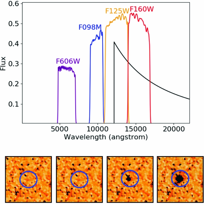
In the top panel of Figure 2, we show the spectrum of a simulated galaxy with β = −2.0 at z = 10.0 with the filters F098M, F125W, F160W, and F606W from HST used in the BoRG survey (described in Section 4.1). The bottom panel shows that same source added to the science images in those filters. It can be seen that there is no image of the artificial galaxy in the F098M and F125W bands, as no flux is expected at these wavelengths, while the artificial source is present in F125W and F160W bands with different intensities, since the Lyman-break falls in the F125W filter.
Top: Spectrum of a simulated galaxy at z = 10 and with β = −2.0 produced by GLACiAR in arbitrary units of flux as a function of wavelength, with four HST filter transmission curves superimposed (F098M, F125W, F160W, and F606W). Bottom: Source from above inserted into the F606W, F098M, F125W, and F160W science images (from left to right) from field BoRG-0835+2456 assuming a n = 4 surface brightness profile and m AB = 24.0 with no inclination and circular shape. The stamps have a size of 3.6~arcsec ×3.6 arcsec.
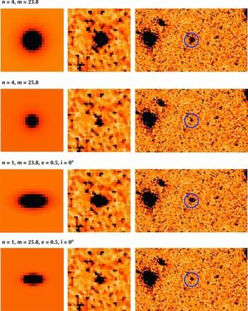
The user can choose different Sérsic indexes for the simulated galaxies as well as the fraction of each type. The default values are 50% of the sources with n = 1, and 50% with n = 4. In terms of morphology, the galaxies can have different inclinations and eccentricities. The inclinations can vary from 0° to 90°, and the user can specify the sampling sequence in the angular coordinate space. For example, if 10 values are chosen, the sampling spacing will be 9°. The same principle applies to eccentricities, whose values vary from 0 (circle) to almost 1 (highly elliptical). Furthermore, we allow for a special case: a Sérsic index of n = 4. This profile (de Vaucouleurs Reference de Vaucouleurs1948) is commonly associated with elliptical galaxies, which tend to have a circular shape. Accordingly, if one of the Sérsic indexes required by the user is n = 4, there is a boolean parameter which indicates whether these galaxies will have only a circular shape, or an elliptical shape (which allows different inclination and eccentricity values). Figure 3 shows examples of simulated galaxies with different features.
Example of different types of galaxies produced by GLACiAR. The left panels show a zoom of the galaxies placed on a constant background (box size 35×35 pixels), while the middle and right panels show them inserted in a typical science image (F160W for the field BoRG-0835+2456) with box sizes (2.8arcsec ×2.8 arcsec and 5.0~arcsec ×2.8 arcsec, respectively). From top to bottom, we see an artificial galaxy with a Sérsic index of 4, and total input magnitude m AB = 23.8; an artificial galaxy with Sérsic index of 4, and magnitude m AB = 25.8; an artificial galaxy with Sérsic index of 1, magnitude m AB = 23.8, eccentricity of 0.5, and inclination angle of 05°; and an artificial galaxy with Sérsic index of 1, magnitude m AB = 25.8, eccentricity of 0.5, and inclination angle of 0°. The first two ones have a circular shape, while the latter two are elliptical.
For each redshift bin, we create a set of stamps each representing an artificial galaxy with total flux given by equation (2). The value of the flux in each individual pixel at position (x i, y i) and size Δr is calculated numerically by integrating the surface brightness profile:
 $$\begin{equation}
L(x_i,y_i) = \int _{x_i-\Delta r/2}^{x_i+ \Delta r/2} \int _{y_i -\Delta r/2}^{y_i + \Delta _r/2} I(r) \text{d}x \text{d}y,
\end{equation}$$
$$\begin{equation}
L(x_i,y_i) = \int _{x_i-\Delta r/2}^{x_i+ \Delta r/2} \int _{y_i -\Delta r/2}^{y_i + \Delta _r/2} I(r) \text{d}x \text{d}y,
\end{equation}$$
where r 2 = (x 2 + y 2).
We note that previous approaches to completeness simulations have resorted to oversampling the inner pixels of the artificial sources as a balance between accuracy and computational speedup (e.g. Peng et al. Reference Peng, Ho, Impey and Rix2002; Häussler et al. Reference Häussler2007). However, as GLACiAR is tailored for high-redshift galaxies, which are typically marginally resolved, we prefer to implement a highly accurate calculation of the flux in each individual pixel.
The artificial sources generated by GLACiAR do not include Poisson noise. This is motivated by the fact that Poisson noise becomes dominant over other components (background, readout, and dark current noise) only in a regime where the source is detected at high confidence (S/N ≳ 50). Under these conditions, completeness simulations are not required. For example, we verified from the HST WFC3 Exposure Time Calculator that for a compact source in the F160W filter, Poisson noise becomes greater than the sky background at S/N > 80.
For each set of parameters, subsets with all the possible galaxies in terms of inclination and eccentricity for each Sérsic index are generated. All the simulated galaxies in each subset have the same redshift, meaning that the parameters that change, apart from n are the slope β, the input magnitude, eccentricity, and inclination angle. Both β and the input magnitude only modify the flux, i.e. the shape of the surface brightness profile of the simulated galaxy remains the same except for a scaling factor. Hence, we do not need to recalculate the flux in each pixel for these galaxies as we can just apply a global rescaling. In the case of the eccentricity and inclination angle, these parameters change the shape of the source and distribution of its flux. Given that, we generate all possible combinations for each subset with the same Sérsic index and redshift. Note that the redshift also changes the distribution of the flux as we define R eff as a function of z.
2.3. Point spread function convolution
The PSF describes the imaging system response to a point input, and we take it into account to properly include the instrumental response into our model mock galaxies. In order to do this, we need a user-supplied PSF image, which is convolved with the artificial galaxy images through the python module convolution.convolve from Astropy. For commonly used HST filters, we already include Tiny Tim PSF dataFootnote 1 in the ‘psf’ folder. If the user desires to apply GLACiAR to filters not listed in the code, the corresponding files can be added to that folder.
2.4. Positions
After generating the simulated galaxy stamps, their position (x, y) is assigned within the science image. These coordinates (x, y) correspond to the pixel where the centre of the stamp will be placed, and are generated as pairs of uniform random numbers across the pixel range in the science image. Two conditions are required to accept the pair: First, for physical reasons, a simulated galaxy cannot be blended with another simulated galaxy (but no limitation is imposed to blending with sources in the original science image) and second, the centre of the simulated source must fall inside the science image boundaries (technically implemented by requiring the pixel to have a value different from zero in the science image). The artificial source positions generated are saved for comparison in the subsequent steps.
2.5. Multiband data
GLACiAR is structured to handle multiple, user-specified photometric bands. Depending on the redshift of the simulated source and the slope of its spectrum β, synthetic images will have different magnitudes in different bands. To calculate them, the code starts from the spectrum defined in Equation (6) (see Figure 2 for an example), and it convolves it with the relevant filter transmission curve using the function pysysp from the package PyPI. Input files for a set of default HST filters are included in our release. If the user requires a different filter that is not part of the GLACiAR’s sample, they can add it by adding the transmission file in the folder ‘filters’.
After calculating the flux of the simulated source in each filter, the postage stamp image of the artificial galaxy is rescaled to that total flux. In order to save time, we let all the simulated galaxies in a single recovery simulation iteration have the same value of β, so there is no need to repeat the filter convolution for sources at the same redshift, and sample instead a different value of β in each iteration. This saves computational resources without impacting the end results since (1) we employ a sufficient number of iterations (n iter = 100 by default) to sample the β distribution reasonably well, and (2) changes in β produce only relatively small differences in colours (Δm < 0.1) for default input choices. Therefore it is not necessary to sample a different β value for each galaxy.
Finally, the artificial galaxies stamps are added to the science images in the corresponding bands, if their total magnitude in that band is below a critical threshold (m AB ⩽ 50 by default).
2.6. Source identification
We run a source identification software (SExtractor in this case) on the original images, as well as on the new images with the simulated galaxies, to create source catalogues. In order to do that, the user must provide a configuration file under the folder ‘SExtractor_files’. If no file is provided, the software uses the default one, ‘parameters.sextractor’. The filter file also needs to be copied here. We provide one example with the filter ‘gauss_2.0_5x5.conv’.
GLACiAR calls SExtractor to run over all the science images with added artificial sources generated in each iteration; it produces new catalogues and new segmentation maps for each of them. To ease storage space requirements, segmentation maps are deleted after use by default.
To study the recovery fraction, the segmentation map of the original image is compared with the segmentation map of the image containing the simulated galaxies. The positions where the simulated galaxies were placed have been recorded, therefore the new segmentation map values in that position can be checked. It is possible that the new source is not found by SExtractor in the actual position that was placed in, thus we allow a certain margin, examining the values of the new segmentation map over a grid of 3 × 3 pixels centred in the original input position. If any of the values of this grid is not zero, the ID number of the object that is there is saved (i.e. the value of that pixel in the segmentation map). To determine whether that object is blended, we check in the original segmentation map the values of the pixels where the simulated object lies. If any of the pixel values are different from zero, the object is flagged as blended. If the real source blended with the simulated galaxy has an original magnitude fainter than the simulated galaxy input magnitude, we still consider the simulated object successfully recovered. On the other hand, if the original science source is brighter, an extra test is performed. If less than 25% of the pixels of the new object overlap with the original object, and there is a difference smaller than 25% between recovered and input flux of the simulated object, we still consider it as recovered, while if any of these two requirements are not met, we flag the artificial source as not recovered. This is a conservative (and moderately computationally intensive) approach on assessing blending, but it has advantages of taking into full account the arbitrary shape of foreground sources and the extent of the overlap of the segmentation maps when compared to a distance-based approach. We also note that 25% overlap is an arbitrary threshold that we fined-tuned based on experimentation, which users are free to modify.
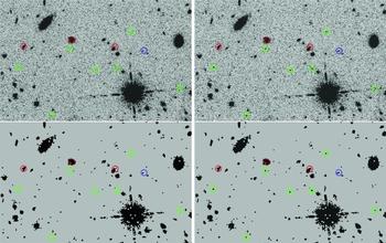
To summarise this process, Figure 4 shows a flow chart with a detailed explanation of, in particular, the blending and recovering of sources. Furthermore, Figure 5 shows an example of the identification of the simulated galaxies in one of the fields of the BoRG survey.
Diagram with a detailed explanation of how GLACiAR’s algorithm structure, focusing in particular on the blending classification.
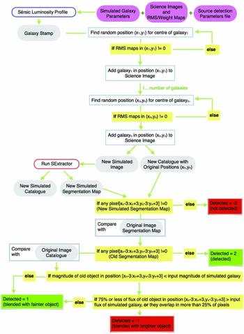
Illustration of GLACiAR’s application to BoRG field  $borg\_$0835+2456. textitTop left: Original science image.Top right: Science image plus simulated galaxies with an input magnitude of m H = 26.0 indicated by coloured circles. Bottom left: SExtractor Segmentation map for the original science image. Bottom right: Segmentation map after running SExtractor on the image that includes simulated galaxies. The colour of the circles encodes detection of the simulated sources with green indicating recovery for an isolated galaxy, blue recovery but source blended with a fainter object. Detection failures are shown in red.
2.7. Multiband photometric output
The ultimate output of GLACiAR is a multiband photometric catalogue that lists input and output properties of the artificial objects, including a flag to indicate whether entries have been marked as successfully recovered. This catalogue naturally allows the user to run a customised data analysis to measure completeness and source recovery using the same criteria that the user would apply to actual science data (whether a dropout technique or a photometric redshift estimation is desired). For convenience of Lyman-break selection users, GLACiAR has a module that performs statistical analysis of the recovery as a function of input redshift and magnitude.
3 IMPLEMENTING AND RUNNING THE CODE
The code is in the Github repository https://github.com/danielacarrasco/GLACiAR. The user should download the code, change the input parameters, and add any files if needed. Detailed instructions are provided in a README file. A brief description of the parameters and required files follows below.
3.1. Input parameters
The parameters needed to run the simulation are found in the file ‘parameters.yaml’. Some of them need to be specified by the user, while others can be either inputted or left blank, in which case they take a default value. A description of all the parameters is given in Appendix A.
3.2. Required files
The files required for the algorithm are described below. More details on their format and location can be found in the README file on Github.
Science images: All the images in which the simulation is going to be run on. It must include all the different fields and bands as well.
List: Text file with the names of the fields from the survey. This list is given as an input parameter (see Section 3.1).
SExtractor parameters: As discussed in Section 2.6, GLACiAR invokes instances of SExtractor on the images (original and with simulated galaxies). To run that external software, a file defining the parameters is needed. There is an example provided under the folder ‘SExtractor_files’ (based on the BoRG survey source detection pipeline), which will be used if no other file is provided, but we recommend the user to customise this input to optimise their specific analysis.
RMS maps or weight maps: Frames having the same size as the science image that describe the noise intensity at each pixel. They are necessary only if required for the SExtractor parameters. They are defined as
(8) $$\begin{equation}
\text{weight} = \frac{1}{\text{variance}} = \frac{1}{\text{rms}^{2}}.
\end{equation}$$
$$\begin{equation}
\text{weight} = \frac{1}{\text{variance}} = \frac{1}{\text{rms}^{2}}.
\end{equation}$$
PSF: PSF data for filters/instruments not currently included in the release can be added in this folder by the user (see Section 2.3 for more details).
4 EXAMPLE APPLICATION
To illustrate GLACiAR’s use, we apply it to estimate the completeness and source recovery of a large HST imaging programme, the BoRG, focused on identifying L > L * galaxies at z ≳ 8 along random lines of sights (Trenti et al. Reference Trenti2011, Reference Trenti2012; Bradley et al. Reference Bradley2012; Schmidt et al. Reference Schmidt2014; Calvi et al. Reference Calvi2016; Bernard et al. Reference Bernard2016). Specifically, we focus on characterising the J-dropout source recovery (galaxies at z ~ 10) and compare our results with those in Bernard et al. (Reference Bernard2016). The results are discussed throughout this section, and they can be seen in Figures 6 and 7.
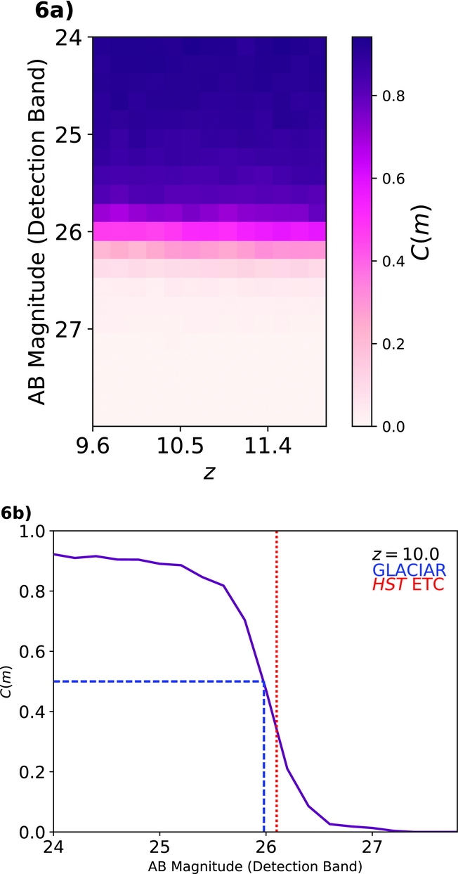
Completeness selection plots produced by our simulation for the BoRG field  $borg\_$0440-5244 in F160W. The top panel shows the completeness for a range of redshifts z = 9.6–12.0, and the bottom panel shows a slice of those results for z = 10. The completeness is around ~90% up to m AB ~ 25.0, and it drops to 0.0% for m AB ≳ 27.0. The blue dashed line shows the 50% calculated by GLACiAR (m AB = 25.98). The red dashed line shows the limiting magnitude at which a point source with circular radius of 0.2 arcsec and a spectrum following a power law F(λ) = λ−1 is detected at a S/N = 8 according to the HST exposure time calculator (m AB = 26.10).
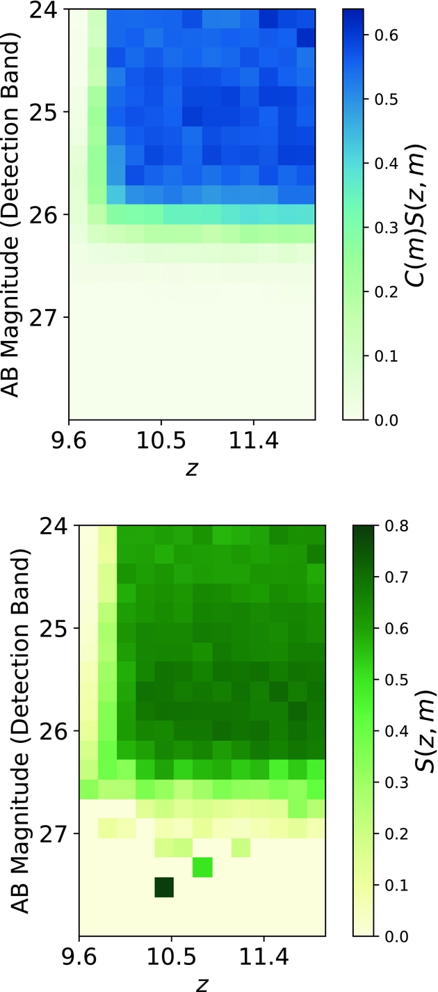
Dropouts selection plots produced by our code for the BoRG field  $borg\_$0440-5244 for redshift z ~ 10. The top panel shows the dropouts found from all the galaxies inserted (C(m)S(z, m)), while the bottom panel shows the fraction of recovered dropouts (S(z, m)) for artificial sources that are successfully identified in the detection band. Note that the bottom panel becomes noisy for m AB > 27.0 since S(z, m) is computed only using the small number of faint artificial galaxies that are identified with success. The top panel does not suffer from such noise, instead.
4.1. Data
The dataset considered here is the BoRG[z8] subset, consisting of core BoRG pointings (GO11700, 12572, 12905), augmented by other pure parallel archival data [GO 11702, PI Yan, Yan et al. (Reference Yan2011)] and COS GTO coordinated parallel observations. For a detailed description of the survey, we refer to Trenti et al. (Reference Trenti2011), Bradley et al. (Reference Bradley2012), and Schmidt et al. (Reference Schmidt2014). We use the 2014 (DR3) public release of the dataFootnote 2, which consists of 71 independent pointings covering a total area of ~350 arcmin2. All fields were imaged in four bands: F098M (Y 098), F125W (J 125), F160W (H 160), and an optical band F606W (V 606) or (V 600). The BoRG[z8] public data release consists of reduced and aligned science images produced with MultiDrizzle (Koekemoer et al. Reference Koekemoer, Fruchter, Hook, Hack, Arribas, Koekemoer and Whitmore2003), a pixel scale of 0.08, and associated weight maps (Bradley et al. Reference Bradley2012; Schmidt et al. Reference Schmidt2014). The 5σ limiting magnitudes for point sources and aperture r = 0.2 arcsec vary between m AB = 25.6 − 27.4, with a typical value of m AB ~ 26.7.
4.2. Redshift selection/dropouts criteria
We use GLACiAR for recovery of simulated sources in the redshift range of z ~ 10. In order to do this, we apply a selection criteria to find J 125 dropouts following Bernard et al. (Reference Bernard2016):
– S/N 160 ⩾ 8.0.
– S/N V < 1.5.
– S/N 098 < 1.5.
– J 125 − H 160 > 1.5.
Note that while these criteria are set as default in the code, their selection is fully customisable by the user.
4.3. Completeness and source recovery output
The main results produced by the program can be summarised in three tables described below, including an example for the first two (see Tables 1 and 2).
Example of the file produced by the simulation with the statistics for each redshift and magnitude.
aInput redshift of the simulated galaxy.
bMagnitude bin that represents the median value of the bins.
cNumber of objects inputted for that redshift and magnitude bin in all the iterations.
dNumber of galaxies recovered by SExtractor that were isolated.
eNumber of artificial sources recovered that were blended with a fainter object.
fNumber of artificial sources recovered that were blended with a brighter object.
gNumber of artificial sources that were detected by SExtractor but with a S/N under the required threshold.
hNumber of artificial sources that were not detected by SExtractor.
iNumber of recovered artificial sources: (d + e).
jNumber of artificial sources that passed the dropout selection criteria.
kFraction of not recovered artificial sources :  $\frac{i}{c}$.
lFraction of artificial sources that passed the selection criteria $\frac{j}{c}$.
Example of the file produced by the GLACiAR with information of all the simulated galaxies.
aMagnitude corresponding to the input flux for the star. This is not the same as das the input magnitude changes depending on the β value and size of the object.
bIteration number.
cIdentification number given by SExtractor after it runs on the image with the simulated galaxies. This number is unique for every iteration for a given magnitude and redshift.
dMagnitude corresponding to the added flux inside all the pixels that the source includes.
eMagnitude of the source found with SExtractor after it runs on the image with the simulated galaxies.
fInteger number that indicates whether a source has been recovered and/or is blended.
First, the statistics of what fraction of the galaxies placed in the image were identified and how many were recovered at the corresponding redshift with the selection technique. Table 1 shows an example of its structure for our BoRG dataset.
Second, a table with more detail about the galaxies that were inserted and the recovering results, several tables (one for each redshift step) are produced with all the galaxies that were placed in the simulations at that redshift. They have the recovered magnitude in the detection band, the identification status, the ID given by SExtractor, among others. The structure is shown in Table 2.
Third, one last table, which is useful for redshift selection. Given that the number of bands is variable, and it can be large, this table is released in a Python-specific compact binary representation (using the pickle module). It contains the ID of the object, input magnitude, status, magnitudes in all bands, and S/N for each band as well.
4.4. Results and comparisons
We run the simulation for the whole BoRG[z8] survey. As an example, the results for one field ( $borg\_$0440-5244) are shown in Figure 6; Figure 6 a shows the completeness fraction C(m) for different redshifts as a function of the input magnitude, while Figure 6 b is a slice of C(m) at a fixed redshift (z = 10.0). As we can see, the completeness is around C(m) ~ 90% up to a magnitude of m AB ~ 25.0, and it drops to C(m) = 0.0% for m AB ≳ 27.1, while at m AB ~ 25.98, we find a completeness of C(m) = 50%. This is expected from when comparing with the results from HST exposure time calculatorFootnote 3: a galaxy at z = 10.0 in an image with the characteristics of the field we are running our simulations on, gives as a S/N ratio of ~8.0 at a magnitude of m AB = 26.1 in the H 160 band for a point source galaxy with circular radius of 0.2 arcsec and a power law F(λ) = λ−1 spectrum.
The results of the dropout selection for the same field are shown in Figure 7. We can compare our results with the ones from Bernard et al. (Reference Bernard2016) (bottom panel of Figure 4 in their paper), where we can see the selection function C(m)S(z, m) for the field  $borg\_$0440-5244. Our results achieve a maximum of ~64% recovery, to be compared against the maximum ~75% recovery reported in their paper. As we have full access to the code used to produce both sets of results, we can attempt to understand the origin of this discrepancy. First of all, there is a difference in C(m) in the range of m AB = 25.5–26.0, that is most likely attributed to the definition of successful recovery for blended or potentially blended sources. In fact, when comparing the results for recovery of isolated objects GLACiAR obtains the same results. The completeness analysis in Bernard et al. (Reference Bernard2016) considers sources as blended based on the distance from the center of the objects, i.e. if the detected object is closer than a certain distance (in pixels) from the centre of an object in the original science catalogue, then it classifies the artificial source as blended. In this respect, GLACiAR improves upon the previous analysis by carrying out a more sophisticated analysis based on comparison of the segmentation maps, which take into account the actual spatial extension of the sources, instead of limiting the analysis to catalogue output.
Another key difference originates from how our galaxies are simulated: we simulate images in all the bands, even when the expected is negligible given the spectrum of the artificial source. In the case of Bernard et al. (Reference Bernard2016), the V-band (F600LP or F606W) non-detection requirement was not simulated since it was assumed that artificial sources had no flux in that band. To account for this, the selection function computed excluding the V-band non-detection requirement was reduced by 6.2%, which derives from the assumption that the S/N distribution in the V-band photometry would follow Gaussian statistics. GLACiAR performs instead a full colour simulation and our results indicate that non-Gaussian tails contribute to exclude a larger fraction of objects at bright magnitudes. Indeed, if we replicate the approach by Bernard et al. (Reference Bernard2016), we obtain instead results consistent with that study (for isolated sources). Thus, all differences are understood and the comparison contributes to validate the accuracy of GLACiAR.
Note that GLACiAR results for C(m) and S(z, m) are provided as a function of the intrinsic magnitude of the simulated images. Previous studies, including Bernard et al. (Reference Bernard2016), may present completeness as a function of recovered output magnitude instead. Since in the latter case, a specific LF for the simulated sources has to be assumed to map intrinsic to observed completeness through a transfer function, we opted to setup the output of GLACiAR to provide only the fundamental quantity, and leave derivation of an observed completeness to the user if needed.
5 DISCUSSION AND SUMMARY
In this paper, we present a new tool to estimate the completeness in galaxy surveys, GLACiAR. This algorithm creates an artificial galaxy stamp that follows a Sérsic profile with parameters such as the size, Sérsic index, input magnitude, input redshift, filters, among others, that are chosen by the user. After creating the galaxies, they are added to the science image. A source identification algorithm is run on the science images and on the images with the simulated galaxies, in order to study the recovery of these mock galaxies. After the source catalogues are produced, we match the newly found objects with the positions in which the simulated galaxies were originally inserted, and we cross-match the area of the segmentation maps corresponding to these new sources with the ones from the original catalogues, so the status of these galaxies can be determined. These statuses can be categorised in four groups: detected and isolated, blended with fainter object, blended with brighter object, and not detected. If a source falls into one of the two first categories only, it is considered detected (an example can be seen in Figure 5). The final product of the algorithm are three types of tables, with the information of the statistics about the recovery, the detected galaxies, and all the galaxies. To illustrate the use of the new tool, and to validate it against previous literature analysis, we applied GLACiAR to analysis of the selection function for z ~ 10 galaxies in the BoRG[z8] survey, comparing our results to the recent work by Bernard et al. (Reference Bernard2016). Section 4 discusses the comparison in detail, with the key summary being that while (minor) differences are present, these can be attributed to improvements introduced by GLACiAR and are fully understood. In particular, the improved completeness analysis is more realistic in its treatment of non-Gaussian noise for all survey bands, and includes a sophisticated comparison between segmentation maps to identify blended objects to high reliability.
This initial application demonstrates that GLACiAR is a valuable tool to unify the completeness estimation in galaxy surveys. So far, the code is limited to surveys where the detection of the sources is done by SExtractor, but its structure has been designed to allow a future upgrade of capabilities by inclusion of photutils as well. More broadly, the code is flexible allowing, for instance, the possibility of modifying the redshift selection criteria along with the fraction of galaxies that follow different values of n for the Sérsic luminosity profile. This makes GLACiAR suitable for a range of different applications in galaxy formation and evolution observations, including studies of LFs, contamination rates in galaxy surveys, characteristics of selected galaxies in redshift selections, among others. A future release of the code will also incorporate a module to account for weak and strong lensing magnification maps, with applications to galaxy cluster surveys such as the Frontier Fields initiative.
ACKNOWLEDGEMENTS
We thank the referee for helpful suggestions and comments that improved the paper. This work was partially supported by grants HST/GO 13767, 12905, and 12572, and by the ARC Centre of Excellence for All-Sky Astrophysics in 3 Dimensions (ASTRO-3D).
A Description of input parameters
Below, there is a list with a brief description of all the parameters used to run GLACiAR:
n_galaxies: Number of galaxies per image to place in each iteration (
$\texttt {default} = 100$).n_iterations: Number of iterations, i.e. the number of times the simulation is going to be run on each image for galaxies with the same redshift and magnitude (
$\texttt {default} = 100$).mag_bins: The number of desired magnitude bins. For a simulation run from m 1 = 24.0 to m 2 = 25.0 in steps of 0.2 magnitudes, there will be six bins (
$\texttt {default} =\break 20$).min_mag: Brightest magnitude of the simulated galaxies (
$\texttt {default} = 24.1$).max_mag: Faintest magnitude of the simulated galaxies (
$\texttt {default} = 27.9$).z_bins: The number of desired redshift bins. For a simulation run from z 1 = 9.5 to z 2 = 10.5 in steps of 0.2, there will be six bins (
$\texttt {default} = 15$).min_z: Minimum redshift of the simulated galaxies (
$\texttt {default} = 9.0$).max_z: Maximum redshift of the simulated galaxies (
$\texttt {default} = 11.9$).n_bands: Number of filters the survey images have been observed in. If not specified, it will raise an error.
detection_band: Band in which objects are identified. If not specified, it will raise an error.
lambda_detection: Central wavelength in angstroms of the detection band. If not specified, it will raise an error.
bands: Name of the bands from n_bands. The detection band has to be the first entry in the list. If not specified, it will raise an error.
zeropoints: Zeropoint values corresponding to each band. The entries must follow the same order as bands. Default values are set as 25.0.
gain_values: Gain values for each band. The entries must follow the same order as bands. If not specified, it will raise an error.
list_of_fields: Text file containing a list with the names of the fields the simulation will run for, which can be one or more. If not specified, it will raise an error.
R_eff: Effective radius in kpc for a simulated galaxy at z = 6. It is the half light radius, i.e. the radius within half of the light emitted is enclosed. This value changes with the redshift as (1 + z)−1 (
$\texttt {default} = 1.075$ kpc).beta_mean: Mean value for a Gaussian distribution of the UV spectral slope (Section 2.2) (
$\texttt {default} = -2.2$).beta_sd: Standard deviation for the for a Gaussian distribution of the slope of the spectrum as explained in Section 2.2 (
$\texttt {default} = 0.4$).size_pix: Pixel scale for the images in arcsec (
$\texttt {default} = 0.08$).path_to_images: Directory where the images are located. The programme will create a folder inside it with the results. If not specified, it will raise an error.
image_name: Name of the images. They all should have the same name with the name of the field (list_of_fields) and band written at the end, as follows: ‘image
$\_$name+field+band.fits’. If not specified, it will raise an error.types_galaxies: Number indicating the amount of Sérsic indexes (
$\texttt {default} = 2$).sersic_indexes: Value of the Sérsic index parameter n for the number of types_galaxies (
$\texttt {default} = [1,4]$).fraction_type_galaxies: Fraction of galaxies corresponding the Sérsic indexes given (
$\texttt {default} = [0.5,0.5]$).ibins: Number of bins for the inclination angle. The inclinations can vary from 0° to 90°, i.e. if 10 bins are chosen, the variations will be of 9°. One bin indicates no variation of inclination angle (
$\texttt {default} = 1$).ebins: Number of bins for the eccentricity. The values can vary 0 to 1, i.e. if 10 bins are chosen, the variations will be of 0.1. One bin indicates only circular shapes (
$\texttt {default} = 1$).min_sn: Minimum S/N ratio in the detection band for an object to be considered detected by SExtractor (
$\texttt {default} = 8.0$).dropouts: Boolean that indicates whether the user desires to run a dropout selection (
$\texttt {default} = {\rm False}$).de_Vacouleur: Boolean that indicates whether the user wants to make an exemption for de Vaucouleur galaxies. If true, galaxies with n = 4 will only have circular shape (
$\texttt {default} = {\rm False}$).