


1. Introduction
1.1 Motivation
Loss severity distributions and aggregate loss distributions in insurance often have a shape that cannot easily be modelled with the common distributions implemented in software packages. In the range of smaller losses and around the mean the observed densities often look somewhat like asymmetric bell curves, being skewed to the right with one positive mode. This is not a problem in itself as well-known models like the Lognormal distribution have exactly this kind of geometry. Alternatively, distributions like the Exponential are available for cases where a strictly decreasing density seems more adequate. However, it often occurs that the traditional models, albeit incorporating the desired kind of skewness towards the right, have a less heavy tail than what the data indicate (Punzo et al., Reference Punzo, Bagnato and Maruotti2018) – if we restrict the fit to the very large losses, the Pareto distribution or variants thereof often seem the best choice. But, those typical heavy-tailed distributions rarely have a shape fitting well below the tail area.
In practice, bad fits in certain areas can sometimes be ignored. When we are mainly focused on the large majority of small and medium losses, we can often accept a bad tail fit and work with, for example, the Lognormal distribution. It might have a tail that is too light, so we will underestimate the expected value; however, often the large losses are such rare that their numerical impact is very low. Conversely, when we are focused on extreme quantiles like the 200-year event or want to rate a policy with a high deductible or a reinsurance layer, we only need an exact model for the large losses. In such situations we could work with a distribution that models smaller losses wrongly (or completely ignores them). There is a wide range of situations where the choice of the model can be made focusing just on the specific task to be accomplished, while some inaccuracy in less important areas is willingly accepted.
However, exactness over the whole range of loss sizes, from the many smaller to the very few large ones, becomes more and more important. For example, according to a modern holistic risk management/capital modelling perspective we do not only look at the average loss (which often depends mainly on the smaller losses) but also want to derive the probability of very bad scenarios (which depend heavily on the tail) – namely, out of the same model. Further, it has become popular to study various levels of retentions for a policy, or for a portfolio to be reinsured. A traditional variant of this is what reinsurers call exposure rating, see, for example, Parodi (Reference Parodi2014), Mack & Fackler (Reference Mack and Fackler2003). For such analyses one needs a distribution model being accurate both in the smaller loss area, which is where the retention typically applies, and in the tail area, whose impact on the expected loss becomes higher the higher the retention is chosen. In other words: one needs a flexible full model with a heavy tail.
Such situations require actuaries to abandon the distribution models they know best and proceed to somewhat more complex ones. In the literature and in software packages there is no lack of such models. For example, the seminal book by Klugman et al. (Reference Klugman, Panjer and Willmot2008) provides generalisations of the Gamma and the Beta distribution having up to four parameters and providing the desired geometries. However, despite the availability of such models, actuaries tend to stick to their traditional distributions. This is not (only) due to nostalgia – it has to do with a common experience of actuarial work: lack of empirical data. In an ever changing environment it is not easy to gather a sufficient amount of representative data to reliably infer several distribution parameters. A way to detect and possibly avoid big estimation errors is to check the inferred parameters with market experience, namely with analogous results calculated from other empirical data stemming from similar business. It would be best to see at a glance whether the inferred parameters are realistic, which means in particular that the parameters must be interpretable in some way.
To this end, it would be ideal to work with models looking initially like one of the traditional distributions but having a tail shape like Pareto with interpretable parameters. Such models can be constructed by piecewise definition on the lower versus large-loss areas; they are called spliced or composite distributions.
1.2 Scientific context
Spliced models have been treated in the applied statistics literature for some decades, see the survey paper by Scarrott & MacDonald (Reference Scarrott and MacDonald2012) for an early overview. Recently the models have received a lot of attention in actuarial publications. We will discuss references in Section 6; let us highlight just a few here. A simple Lognormal-Pareto variant was presented early by Knecht & Küttel (Reference Knecht and Küttel2003). The seminal paper for the topic is Scollnik (Reference Scollnik2007) proposing a more general Lognormal-Pareto/GPD model that has inspired many authors to study variants thereof, in particular alternatives for the Lognormal part, and to apply them to insurance loss data. Grün & Miljkovic (Reference Grün and Miljkovic2019) give a compact overview of this research, followed by an inventory of over 250 spliced distributions, which were notably all implemented and applied.
1.3 Objective
The main scope of our paper is to collect and generalise a number of spliced models having a Pareto or GPD tail, and to design a general framework of variants and extensions of the Pareto distribution family. Special attention is paid to the geometry of distribution functions and to intuitive interpretations of parameters. We show where such intuition can ease parameter inference from scarce data, e.g. by combining information from different sources.
1.4 Outline
Section 2 explains why reinsurers like the single-parameter Pareto distribution so much, and collects some results that enhance intuition about distribution tails in general. Section 3 presents parameterisations of the Generalised Pareto distribution that will make reinsurers (and some others) like this model too. Section 4 explains how more Pareto variants can be created, catering in particular for a more flexible modelling of smaller losses. Section 5 gives an inventory of spliced Lognormal-Pareto models that embraces as special cases various distributions introduced earlier by other authors. Section 6 reviews analogous models employing other distributions in place of Lognormal, plus some generalisations. Section 7 revisits the Riebesell model and another old exposure rating method, in the light of the methodology developed so far.
The sections are somewhat diverse, from mixed educational-survey (2, 3, 4) to mainly literature survey (6) to original research (5, 7). All content, be it well known, less common or novel, is presented with the same practice-oriented aim: to provide intuition for models that can help in scarce-data situations.
This paper emerges from an award-winning conference paper (Fackler, Reference Fackler2013), providing updated and additional content. In particular, we treat the full range of the GPD, not only the popular Pareto-like case having the exponent
 $$\xi \gt 0$$
. Further we appraise the fast-growing literature on spliced models by discussing both older and recent references.
$$\xi \gt 0$$
. Further we appraise the fast-growing literature on spliced models by discussing both older and recent references.
1.5 Technical remarks
In most of the following we will not distinguish between loss severity and aggregate loss distributions. Technically, model fitting works the same way, further the shapes being observed for the two distribution types overlap. For aggregate losses, at least in case of large portfolios and not too many dependencies between the single risks, it is felt that distributions should mostly have a unique positive mode (maximum density) like the Normal distribution; however, considerable skewness and heavy tails cannot be ruled out (Knecht & Küttel, Reference Knecht and Küttel2003). Severity distributions are observed to be more heavy-tailed; here a priori both a strictly decreasing density and a positive mode are plausible, let alone multimodal distributions requiring very complex modelling (Klugman et al., Reference Klugman, Panjer and Willmot2008).
For any loss severity or aggregate loss distribution, let
 $$\bar F\left( x \right) = 1 - F\left( x \right) = {\rm{P}}\left( {X \gt x} \right)$$
be the survival function,
$$\bar F\left( x \right) = 1 - F\left( x \right) = {\rm{P}}\left( {X \gt x} \right)$$
be the survival function,
 $$f\left( x \right)$$
the probability density function (where it exists), that is, the derivative of the cumulative distribution function
$$f\left( x \right)$$
the probability density function (where it exists), that is, the derivative of the cumulative distribution function
 $$F\left( x \right)$$
. As it is geometrically more intuitive (and a bit more general), we will formulate as many results as possible in terms of cdf instead of pdf, mainly working with the survival function, which often yields simpler formulae than the cdf.
$$F\left( x \right)$$
. As it is geometrically more intuitive (and a bit more general), we will formulate as many results as possible in terms of cdf instead of pdf, mainly working with the survival function, which often yields simpler formulae than the cdf.
Unless specified otherwise, the model parameters appearing in this paper are (strictly) positive real numbers.
2. Pareto – reinsurer’s old love
One could call it the standard model of the reinsurance pricing actuaries: The Pareto distribution, also called Type I Pareto, European Pareto, or Single-parameter Pareto, has survival function $\bar F\left( x \right) = {\left( {{\theta \over x}} \right)^\alpha },\;\;\;\;\theta \le x.$
In this paper we reserve the name “Pareto” for this specific model, noting that is used for other variants of the large Pareto family as well.
Does the Pareto model have one or two parameters? It depends – namely on what the constraint
 $$\theta \le x$$
means. It may mean that no losses between
$$\theta \le x$$
means. It may mean that no losses between
 $$0$$
and
$$0$$
and
 $$\theta $$
exist, or alternatively that nothing shall be specified about losses between
$$\theta $$
exist, or alternatively that nothing shall be specified about losses between
 $$0$$
and
$$0$$
and
 $$\theta $$
. Unfortunately, this is not always clearly mentioned when the model is used. Formally, we have two very different cases:
$$\theta $$
. Unfortunately, this is not always clearly mentioned when the model is used. Formally, we have two very different cases:
Situation 1: There are no losses below the threshold
 $$\theta $$
.
$$\theta $$
.
This model has two parameters
 $$\alpha $$
und
$$\alpha $$
und
 $$\theta $$
. Here
$$\theta $$
. Here
 $$\theta $$
is not just a parameter, it is indeed a scale parameter (as defined e.g. in Klugman et al., Reference Klugman, Panjer and Willmot2008) of the model.
$$\theta $$
is not just a parameter, it is indeed a scale parameter (as defined e.g. in Klugman et al., Reference Klugman, Panjer and Willmot2008) of the model.
We call the above model Pareto-only, reflecting the fact that there is no area of small losses having a distribution shape other than Pareto.
This model is quite popular, despite its unrealistic shape in the area of low losses, whatever
 $$\theta $$
is. (If
$$\theta $$
is. (If
 $$\theta $$
is large, there is an unrealistically large gap in the distribution. If
$$\theta $$
is large, there is an unrealistically large gap in the distribution. If
 $$\theta $$
is small, say
$$\theta $$
is small, say
 $$\theta = 1$$
Euro, the gap is negligible, but a Pareto-like shape for losses in the range from
$$\theta = 1$$
Euro, the gap is negligible, but a Pareto-like shape for losses in the range from
 $$1$$
to some 10,000 Euro is rarely observed in the real world.)
$$1$$
to some 10,000 Euro is rarely observed in the real world.)
Situation 2: Only the tail is modelled, so to be precise we are dealing with the conditional distribution
 $$\bar F\left( {x\left| {X \gt \theta } \right.} \right) = {\left( {{\theta \over x}} \right)^\alpha },\;\;\;\;\;\;\;\;\theta \le x.$$
This model only has parameter
 $$\alpha $$
, while
$$\alpha $$
, while
 $$\theta $$
is the known lower threshold of the model.
$$\theta $$
is the known lower threshold of the model.
Situation 1 implies Situation 2 but not vice versa. We will later see distributions combining a Pareto tail with a quite different distribution of the smaller losses.
2.1 A memoryless property
Why is the Pareto model so popular among reinsurers? The most useful property of the Pareto tail model is without doubt the closedness and parameter invariance when modelling upper tails: if we have
 $$\bar F\left( {x\left| {X \gt \theta } \right.} \right) = {\left( {{\theta \over x}} \right)^\alpha }$$
and derive the model for a higher threshold
$$\bar F\left( {x\left| {X \gt \theta } \right.} \right) = {\left( {{\theta \over x}} \right)^\alpha }$$
and derive the model for a higher threshold
 $$d \ge \theta $$
, we get
$$d \ge \theta $$
, we get
 $$\bar F\left( {x\left| {X \gt d} \right.} \right) = {{\bar F\left( {x\left| {X \gt \theta } \right.} \right)} \over {\bar F\left( {d\left| {X \gt \theta } \right.} \right)}} = {{{{\left( {{\theta \over x}} \right)}^\alpha }} \over {{{\left( {{\theta \over d}} \right)}^\alpha }}} = {\left( {{d \over x}} \right)^\alpha },\;\;\;\;\;\;\;\;d \le x,$$
which is again Pareto with
 $$d$$
taking the place of
$$d$$
taking the place of
 $$\theta $$
. We could say, when going “upwards” to model somewhat larger losses only, the model “forgets” the original threshold
$$\theta $$
. We could say, when going “upwards” to model somewhat larger losses only, the model “forgets” the original threshold
 $$\theta $$
, which is not needed any further – instead the new threshold comes in. That implies:
$$\theta $$
, which is not needed any further – instead the new threshold comes in. That implies:
• If a distribution has a Pareto tail and we only need to model quite large losses, we do not need to know exactly where that tail starts. As long as we are in the tail (let us call it Pareto area) we always have the same parameter
 $$\alpha $$
, no matter which threshold is used.
$$\alpha $$
, no matter which threshold is used.• It is possible to compare data sets having different (reporting) thresholds. Say for a MTPL portfolio we know all losses above
$$2$$
million Euro, for another one we only have the losses exceeding
$$3$$
million Euro available. Although these tail models have different thresholds, we can judge whether the underlying portfolios have similar tail behaviour or not, according to whether they have similar Pareto alphas. Such comparisons of tails starting at different thresholds are extremely useful in the reinsurance practice, where typically, to get a representative overview of a line of business in a country, one must collect data from several reinsured portfolios, all possibly having different reporting thresholds.• This comparability across tails can lead to market values for Pareto alphas being applicable as benchmarks: see Schmutz & Doerr (Reference Schmutz and Doerr1998) and Section 4.4.8 of FINMA (2006). Say we observe that a certain type of Fire portfolio in a certain country frequently has Pareto tails starting somewhere between
$$1$$
and
$$2$$
million Euro, having an alpha typically in the range of
$$1.8$$
.


With the option to compare an inferred Pareto alpha to other fits or to market benchmarks, it becomes an interpretable parameter.
2.2 Basic formulae
Let us recall some useful facts about losses in the Pareto tail (Schmutz & Doerr, Reference Schmutz and Doerr1998). These are well known but we will show some less-known generalisations soon.
2.2.1 Pareto extrapolation equation for frequencies
To relate frequencies at different thresholds
 $${d_1},{d_2} \ge \theta $$
, the Pareto model yields a famous, very simple, equation, called Pareto extrapolation:
$${d_1},{d_2} \ge \theta $$
, the Pareto model yields a famous, very simple, equation, called Pareto extrapolation:
 $${{{\rm{frequency}}\;{\rm{at}}\;{d_2}} \over {{\rm{frequency}}\;{\rm{at}}\;{d_1}}} = {\left( {{{{d_1}} \over {{d_2}}}} \right)^\alpha }$$
2.2.2 Structure of layer premiums
Consider a (re)insurance layer
 $$C{\rm{\;xs\;}}D$$
, that is, a cover paying, of each loss
$$C{\rm{\;xs\;}}D$$
, that is, a cover paying, of each loss
 $$x$$
, the part
$$x$$
, the part
 $${\rm{min}}\left( {{{\left( {x - D} \right)}^ + },C} \right)$$
. (Infinite
$${\rm{min}}\left( {{{\left( {x - D} \right)}^ + },C} \right)$$
. (Infinite
 $$C$$
is admissible for
$$C$$
is admissible for
 $$\alpha \gt 1$$
.) Suppose the layer operates fully in the Pareto area, that is,
$$\alpha \gt 1$$
.) Suppose the layer operates fully in the Pareto area, that is,
 $$D \ge \theta $$
. Then the average layer loss equals
$$D \ge \theta $$
. Then the average layer loss equals
 $${\rm{E}}\left( {{\rm{min}}\left( {X - D,C} \right)\left| {X \gt D} \right.} \right) = {D \over {\alpha - 1}}\left( {1 - {{\left( {1 + {C \over D}} \right)}^{1 - \alpha }}} \right)\;\;\;\;{\underset{\mathop\alpha \to 1}{\longrightarrow}}\;\;\;\;D \, {\rm{ln}}\left( {1 + {C \over D}} \right),$$
which is well-defined (taking the limit) also for
 $$\alpha = 1$$
.
$$\alpha = 1$$
.
If
 $$\eta $$
is the loss frequency at
$$\eta $$
is the loss frequency at
 $$\theta $$
, the frequency at
$$\theta $$
, the frequency at
 $$D$$
equals
$$D$$
equals
 $$\eta {\left( {{\theta \over D}} \right)^\alpha }$$
. Thus, the risk premiums of layers have a particular structure, equalling a function
$$\eta {\left( {{\theta \over D}} \right)^\alpha }$$
. Thus, the risk premiums of layers have a particular structure, equalling a function
 $${D^{1 - \alpha }}\psi \left( {{D \over C}} \right)$$
. This yields a further simple extrapolation equation.
$${D^{1 - \alpha }}\psi \left( {{D \over C}} \right)$$
. This yields a further simple extrapolation equation.
2.2.3 Pareto extrapolation equation for layer risk premiums
 $${{{\rm{risk}}\;{\rm{premium}}\;{\rm{of}}\;{C_2}{\rm{xs}}{D_2}} \over {{\rm{risk}}\;{\rm{premium}}\;{\rm{of}}\;{C_1}{\rm{xs}}{D_1}}} = {{{{\left( {{C_2} + {D_2}} \right)}^{1 - \alpha }} - D_2^{1 - \alpha }} \over {{{\left( {{C_1} + {D_1}} \right)}^{1 - \alpha }} - D_1^{1 - \alpha }}}\;\;\;\;{\underset{\mathop\alpha \to 1}{\longrightarrow}} \;\;\;\;{{{\rm{ln}}\left( {1 + {{{C_2}} \over {{D_2}}}} \right)} \over {{\rm{ln}}\left( {1 + {{{C_1}} \over {{D_1}}}} \right)}}$$
2.3. Testing empirical data
Distributions having nice properties only help if they provide good fits to real-world data. From the (re)insurance practice it is known that not all empirical tails look like Pareto; in particular the model often seems to be somewhat too heavy-tailed at the very large end, see Albrecher et al. (Reference Albrecher, Araujo-Acuna and Beirlant2021) for Pareto modifications catering for this effect. Nevertheless Pareto can be a good model for a wide range of loss sizes. For example, if it fits well between
 $$1$$
and
$$1$$
and
 $$20$$
million Euro, one can use it for layers in that area independently of whether or not beyond
$$20$$
million Euro, one can use it for layers in that area independently of whether or not beyond
 $$20$$
million Euro a different model is needed.
$$20$$
million Euro a different model is needed.
To quickly check whether an empirical distribution is well fit by the Pareto model, at least for a certain range of loss sizes, there is a well-known graphical method available:
•
$$\bar F\left( x \right)$$
is Pareto is equivalent to•
$$\bar F\left( x \right)$$
is a straight line on double-logarithmic paper (having slope –
$$\alpha $$
).


So, if the log-log-graph of an empirical survival function is about a straight line for a certain range of loss sizes, in that area a Pareto fit should work well.
2.4 Local property
Thinking of quite small intervals of loss sizes being apt for Pareto fits leads to a generalisation being applicable to any smooth distribution: the local Pareto alpha (Riegel, Reference Riegel2008). Mathematically, it is the negative derivative of
 $$\bar F\left( x \right)$$
on log-log scale.
$$\bar F\left( x \right)$$
on log-log scale.
At any point
 $$x \gt 0$$
where the survival function is positive and differentiable, we call
$$x \gt 0$$
where the survival function is positive and differentiable, we call
 $${\alpha _x}: = - {\left. {{d \over {dt}}} \right|_{t = {\rm{ln}}\left( x \right)}}{\rm{ln}}\left( {\bar F\left( {{e^t}} \right)} \right) = x{{f\left( x \right)} \over {\bar F\left( x \right)}}$$
the local Pareto alpha at
 $$x$$
.
$$x$$
.
If
 $${\alpha _x}$$
is a constant on some interval, this interval is a Pareto-distributed piece of the distribution. In practice one often, but not always, observes that, for very large
$${\alpha _x}$$
is a constant on some interval, this interval is a Pareto-distributed piece of the distribution. In practice one often, but not always, observes that, for very large
 $$x$$
(far out in the million Euro range),
$$x$$
(far out in the million Euro range),
 $${\alpha _x}$$
is a (slowly) increasing function of
$${\alpha _x}$$
is a (slowly) increasing function of
 $$x$$
. The resulting distribution tail is somewhat less heavy than that of distributions with Pareto tail, where
$$x$$
. The resulting distribution tail is somewhat less heavy than that of distributions with Pareto tail, where
 $${\alpha _x}$$
is constant for large
$${\alpha _x}$$
is constant for large
 $$x$$
.
$$x$$
.
The above Pareto extrapolation equation for frequencies yields an intuitive interpretation of the local Pareto alpha: it is the speed of the decrease of the loss frequency as a function of the threshold. One sees quickly that if we increase a threshold
 $$d$$
by
$$d$$
by
 $$p$$
percent (for small
$$p$$
percent (for small
 $$p$$
), the loss frequency decreases by approximately
$$p$$
), the loss frequency decreases by approximately
 $${\alpha _d}{\rm{\;}}p$$
percent. Or equivalently, if we keep the threshold fixed but the losses increase by
$${\alpha _d}{\rm{\;}}p$$
percent. Or equivalently, if we keep the threshold fixed but the losses increase by
 $$p$$
percent (say due to inflation), the loss frequency at
$$p$$
percent (say due to inflation), the loss frequency at
 $$d$$
increases by approximately
$$d$$
increases by approximately
 $${\alpha _d}{\rm{\;}}p$$
percent. See Chapter 6 of Fackler (Reference Fackler2017) for how this leads to a general theory of the impact of inflation on (re)insurance layers.
$${\alpha _d}{\rm{\;}}p$$
percent. See Chapter 6 of Fackler (Reference Fackler2017) for how this leads to a general theory of the impact of inflation on (re)insurance layers.
3. Generalised Pareto – a new love?
Now we study a well-known generalisation of the Pareto model, see in the following Embrechts et al. (Reference Embrechts, Klüppelberg and Mikosch2013). Apparently less known is that it shares some of the properties making the Pareto model so popular.
The Generalised Pareto distribution, shortly denoted as GP(D), has survival function
 $$\bar F\left( {x\left| {X \gt \theta } \right.} \right) = {\left( {{{\left( {1 + \xi {{x - \theta } \over \tau }} \right)}^ + }} \right)^{ - {1 \over \xi }}},\;\;\;\;\;\;\;\;\theta \le x.$$
This is a tail model like Pareto, having two parameters
 $$\xi $$
und
$$\xi $$
und
 $$\tau $$
, while
$$\tau $$
, while
 $$\theta $$
is the known model threshold. However,
$$\theta $$
is the known model threshold. However,
 $$\theta $$
is the third parameter in the corresponding GP-only model having no losses between
$$\theta $$
is the third parameter in the corresponding GP-only model having no losses between
 $$0$$
and
$$0$$
and
 $$\theta $$
, analogous to the Pareto case.
$$\theta $$
, analogous to the Pareto case.
 $$\xi $$
can take any real value, while
$$\xi $$
can take any real value, while
 $$\tau $$
must be positive. We use
$$\tau $$
must be positive. We use
 $$\tau $$
instead of the more common
$$\tau $$
instead of the more common
 $$\sigma $$
in order to reserve the latter for the Lognormal distribution. The GPD has finite expectation iff
$$\sigma $$
in order to reserve the latter for the Lognormal distribution. The GPD has finite expectation iff
 $$\xi \lt 1$$
. For negative
$$\xi \lt 1$$
. For negative
 $$\xi $$
the losses are (almost surely) bounded, having the supremum
$$\xi $$
the losses are (almost surely) bounded, having the supremum
 $$\theta + {\tau \over { - \xi }}$$
. The case
$$\theta + {\tau \over { - \xi }}$$
. The case
 $$\xi = 0$$
is well defined (take the limit) and yields the Exponential distribution
$$\xi = 0$$
is well defined (take the limit) and yields the Exponential distribution
 $$\bar F\left( {x\left| {X \gt \theta } \right.} \right) = {\rm{exp}}\left( { - {{x - \theta } \over \tau }} \right).$$
We call the case
 $$\xi \gt 0$$
proper GPD.
$$\xi \gt 0$$
proper GPD.
Proper GP is largely considered the most interesting case for the insurance practice. Some authors notably mean only this case when speaking of the GPD.
The parameterisation for the Generalized Pareto distribution in comes from Extreme Value Theory (EVT), which is frequently quoted in the literature to justify the use of the GPD for the modelling of insurance data exceeding large thresholds.
The core of this reasoning is the famous Pickands-Balkema-De Haan Theorem stating that, simply put, for large-enough thresholds, the distribution tail asymptotically equals the GPD; see Balkema & De Haan (Reference Balkema and De Haan1974), Pickands (Reference Pickands1975). It could, however, be that the relevance of this theorem for the insurance practice is a bit overrated. A warning comes notably from a prominent EVT expert (Embrechts, Reference Embrechts2010): the rate of convergence to the GPD can be extremely slow (much slower than one is used to from the Central Limit Theorem), thus could be too slow for practical relevance.
Further, most real-world loss distributions must have limited support. Insured risks usually have finite sums insured, which also limits the loss potential of accumulation losses and aggregate losses. And even where explicit insurance policy limits don’t apply, most losses should be bounded by, say, 300 times today’s world GDP. With such upper bounds, EVT still applies, but here “high-enough threshold” could mean five Dollars less than the upper bound, which would again not be of practical interest.
Whether or not one is optimistic about the applicability of EVT, there are practical reasons for using the GPD. Widespread application in (and beyond) insurance shows that it provides good fits to a lot of tail data. Further, one can make its parameters interpretable, which can be helpful in scarce-data situations. This option emerges from a parameter change proposed by Scollnik (Reference Scollnik2007) for the proper GPD.
Set
 $$\alpha : = {1 \over \xi } \gt 0$$
,
$$\alpha : = {1 \over \xi } \gt 0$$
,
 $$\lambda : = \alpha \tau - \theta \gt - \theta $$
. Now we have
$$\lambda : = \alpha \tau - \theta \gt - \theta $$
. Now we have
 $$\bar F\left( {x\left| {X \gt \theta } \right.} \right) = {\left( {{{\theta + \lambda } \over {x + \lambda }}} \right)^\alpha },\;\;\;\;\;\;\;\;\theta \le x.$$
The parameter space is quite intricate here as
 $$\lambda $$
may (to some extent) take on negative values. So, for parameter inference other parameterisations may work better. Yet, apart from this complication, the above representation will turn out to be extremely convenient, revealing in particular a lot of analogies to the Pareto model.
$$\lambda $$
may (to some extent) take on negative values. So, for parameter inference other parameterisations may work better. Yet, apart from this complication, the above representation will turn out to be extremely convenient, revealing in particular a lot of analogies to the Pareto model.
3.1. Names and parameters
At a glance we note two well-known special cases:
Case 1
 $$\lambda = 0$$
. This is the Pareto tail model from Section 2.
$$\lambda = 0$$
. This is the Pareto tail model from Section 2.
Case 2
 $$\lambda \gt 0$$
,
$$\lambda \gt 0$$
,
 $$\theta = 0$$
. This is not a tail model but a ground-up model (full model) for losses of any size. In the literature it is often called Pareto as well. However, some more specific names have been introduced: Type II Pareto, American Pareto, Two-parameter Pareto, Lomax.
$$\theta = 0$$
. This is not a tail model but a ground-up model (full model) for losses of any size. In the literature it is often called Pareto as well. However, some more specific names have been introduced: Type II Pareto, American Pareto, Two-parameter Pareto, Lomax.
Let us look briefly at a third kind of model. Every tail model reflecting a conditional distribution
 $$X\left| {X \gt \theta } \right.$$
has a corresponding excess model
$$X\left| {X \gt \theta } \right.$$
has a corresponding excess model
 $$X - \theta \left| {X \gt \theta } \right.$$
. If the former is proper GP as above, the latter has the survival function
$$X - \theta \left| {X \gt \theta } \right.$$
. If the former is proper GP as above, the latter has the survival function
 $${\left( {{{\theta + \lambda } \over {x + \theta + \lambda }}} \right)^\alpha }$$
, which is Two-parameter Pareto with parameters
$${\left( {{{\theta + \lambda } \over {x + \theta + \lambda }}} \right)^\alpha }$$
, which is Two-parameter Pareto with parameters
 $$\alpha $$
and
$$\alpha $$
and
 $$\theta + \lambda \gt 0$$
. However, in the Pareto case the survival function
$$\theta + \lambda \gt 0$$
. However, in the Pareto case the survival function
 $${\left( {{\theta \over {x + \theta }}} \right)^\alpha }$$
looks like Two-parameter Pareto but is materially different: here
$${\left( {{\theta \over {x + \theta }}} \right)^\alpha }$$
looks like Two-parameter Pareto but is materially different: here
 $$\theta $$
is the known threshold – this model has the only parameter
$$\theta $$
is the known threshold – this model has the only parameter
 $$\alpha $$
.
$$\alpha $$
.
The names Single versus Two-parameter Pareto (apart from anyway not being always consistently used in the literature) are somewhat misleading – as we have seen, both models have variants having 1 or 2 parameters, respectively. Whatever the preferred name, when using a Pareto variant, it is essential to make always clear whether one is using it as a ground-up model, a tail model, or an excess model.
3.2. Memoryless property
Let us come back to the GP tail model, for which in the following we borrow a bit from Section 6.5 of Fackler (Reference Fackler2017). If we as above derive the model for a higher tail starting at
 $$d \gt \theta $$
, we get
$$d \gt \theta $$
, we get
 $$\bar F\left( {x\left| {X \gt d} \right.} \right) = {{{{\left( {{{\theta + \lambda } \over {x + \lambda }}} \right)}^\alpha }} \over {{{\left( {{{\theta + \lambda } \over {d + \lambda }}} \right)}^\alpha }}} = {\left( {{{d + \lambda } \over {x + \lambda }}} \right)^\alpha },\;\;\;\;\;\;\;\;d \le x.$$
As in the Pareto case, the model is still (proper) GP but “forgets” the original threshold
 $$\theta $$
, replacing it by the new one. Again the parameter
$$\theta $$
, replacing it by the new one. Again the parameter
 $$\alpha $$
remains unchanged but also the second parameter
$$\alpha $$
remains unchanged but also the second parameter
 $$\lambda $$
. Both are thus invariants when modelling higher tails. The standard parameterisation of the GPD has only the invariant parameter
$$\lambda $$
. Both are thus invariants when modelling higher tails. The standard parameterisation of the GPD has only the invariant parameter
 $$\xi $$
, while the second parameter changes in an intricate way when shifting from a tail threshold to another one. There is, however, a variant that is tail invariant and works notably for any real
$$\xi $$
, while the second parameter changes in an intricate way when shifting from a tail threshold to another one. There is, however, a variant that is tail invariant and works notably for any real
 $$\xi $$
: replace
$$\xi $$
: replace
 $$\tau $$
by the so-called modified scale
$$\tau $$
by the so-called modified scale
 $$\omega = \tau - \xi \theta \gt - \xi \theta $$
, see, for example, Scarrott & MacDonald (Reference Scarrott and MacDonald2012). This yields
$$\omega = \tau - \xi \theta \gt - \xi \theta $$
, see, for example, Scarrott & MacDonald (Reference Scarrott and MacDonald2012). This yields
 $$\bar F\left( {x\left| {X \gt \theta } \right.} \right) = {\left( {{{\xi \theta + \omega } \over {{{\left( {\xi x + \omega } \right)}^ + }}}} \right)^{{1 \over \xi }}},\;\;\;\;\;\;\;\;\theta \le x$$
and for higher tails one just has to replace
 $$\theta $$
by the new threshold (which for
$$\theta $$
by the new threshold (which for
 $$\xi \lt 0$$
must be below the supremum loss
$$\xi \lt 0$$
must be below the supremum loss
 $$\theta + {\tau \over { - \xi }} = {\omega \over { - \xi }}$$
).
$$\theta + {\tau \over { - \xi }} = {\omega \over { - \xi }}$$
).
The tail invariance of
 $$\alpha $$
and
$$\alpha $$
and
 $$\lambda $$
, or of
$$\lambda $$
, or of
 $$\xi $$
and
$$\xi $$
and
 $$\omega $$
for the whole GPD, yields the same advantages for tail analyses as the Pareto model – interpretable parameters:
$$\omega $$
for the whole GPD, yields the same advantages for tail analyses as the Pareto model – interpretable parameters:
• There is no need to know exactly where the tail begins,
• one can compare tails starting at different thresholds,
• it might be possible to derive market values for the two parameters in certain business areas.
Thus, one can use the GPD in the same way as the Pareto model. The additional parameter adds flexibility – while on the other hand requiring more data for parameter inference.
The parameters
 $$\alpha \gt 0$$
and
$$\alpha \gt 0$$
and
 $$\lambda = \alpha \omega $$
of the proper GPD have a geometric interpretation:
$$\lambda = \alpha \omega $$
of the proper GPD have a geometric interpretation:
•
$$\lambda $$
is a “shift” from the Pareto model having the same alpha. (Note that
$$\lambda $$
has the same “dimension” as the losses, for example, Euro or thousand US Dollar.) We could think of starting with a Pareto distribution having the threshold
$$\theta + \lambda \gt 0$$
, then all losses are shifted by
$$\lambda $$
to the left (by subtracting
$$\lambda $$
) and we obtain the GPD. Thus, in graphs (with linear axes), proper GP tails have exactly the same shape as Pareto tails; just their location on the x-axis is different.• The parameter
$$\alpha $$
, apart from belonging to the corresponding Pareto model, is the local Pareto alpha at infinite:
$${\alpha _\infty } = \alpha $$
. More generally, one sees quickly that
$${\alpha _d} = {d \over {d + \lambda }}\alpha $$
.


The behaviour of
 $${\alpha _d}$$
as a function of
$${\alpha _d}$$
as a function of
 $$d$$
is as follows:
$$d$$
is as follows:
Case 1
 $$\lambda \gt 0$$
:
$$\lambda \gt 0$$
:
 $${\alpha _d}$$
rises (as is often observed for fits of large insurance losses).
$${\alpha _d}$$
rises (as is often observed for fits of large insurance losses).
Case 2
 $$\lambda = 0$$
: Pareto (
$$\lambda = 0$$
: Pareto (
 $$\theta \gt 0$$
).
$$\theta \gt 0$$
).
Case 3
 $$\lambda \lt 0$$
:
$$\lambda \lt 0$$
:
 $${\alpha _d}$$
decreases (
$${\alpha _d}$$
decreases (
 $$\theta \gt - \lambda \gt 0$$
).
$$\theta \gt - \lambda \gt 0$$
).
For any
 $$d \ge \theta $$
one easily gets
$$d \ge \theta $$
one easily gets
 $$\bar F\left( {x\left| {X \gt d} \right.} \right) = {\left( {1 + {{{\alpha _d}} \over \alpha }\left( {{x \over d} - 1} \right)} \right)^{ - \alpha }},\;\;\;\;\;\;\;\;d \le x,$$
which is an alternative proper-GP parameterisation focusing on the local alphas (Riegel, Reference Riegel2008).
3.3. Proper GPD formulae
Bearing in mind that proper GP is essentially Pareto with the x-axis shifted by
 $$\lambda $$
, we get without any further calculation compact formulae very similar to the Pareto case:
$$\lambda $$
, we get without any further calculation compact formulae very similar to the Pareto case:
 $${{{\rm{frequency}}\;{\rm{at}}\;{d_2}} \over {{\rm{frequency}}\;{\rm{at}}\;{d_1}}} = {\left( {{{{d_1} + \lambda } \over {{d_2} + \lambda }}} \right)^\alpha }$$
 $${\rm{E}}\left( {{\rm{min}}\left( {X - D,C} \right)\left| {X \gt D} \right.} \right) = {{D + \lambda } \over {\alpha - 1}}\left( {1 - {{\left( {1 + {C \over {D + \lambda }}} \right)}^{1 - \alpha }}} \right){\rm{\;\;\;\;}}{\underset{\mathop\alpha = 1}{\longrightarrow}} {\rm{\;\;\;\;}}\left( {D + \lambda } \right){\rm{ln}}\left( {1 + {C \over {D + \lambda }}} \right)$$ ${{{\rm{risk\;premium\;of\;}}{C_2}{\rm{xs}}{D_2}} \over {{\rm{risk\;premium\;of\;}}{C_1}{\rm{xs}}{D_1}}} = {{{{\left( {{C_2} + {D_2} + \lambda } \right)}^{1 - \alpha }} - {{\left( {{D_2} + \lambda } \right)}^{1 - \alpha }}} \over {{{\left( {{C_1} + {D_1} + \lambda } \right)}^{1 - \alpha }} - {{\left( {{D_1} + \lambda } \right)}^{1 - \alpha }}}}{\rm{\;\;\;\;}}{\underset{\mathop\alpha = 1 }{\longrightarrow}} {\rm{\;\;\;\;}}{{{\rm{ln}}\left( {1 + {{{C_2}} \over {{D_2} + \lambda }}} \right)} \over {{\rm{ln}}\left( {1 + {{{C_1}} \over {{D_1} + \lambda }}} \right)}}$
Summing up, proper Generalised Pareto is nearly as easy to handle as Pareto, but has two advantages: greater flexibility and the backing from both Extreme Value Theory and practical experience making it a preferred candidate for the modelling of high tails.
3.4. The complete picture
Formally, the parameters
 $$\alpha $$
and
$$\alpha $$
and
 $$\lambda $$
are not only applicable for the proper GPD but also for
$$\lambda $$
are not only applicable for the proper GPD but also for
 $$\xi \lt 0$$
. However, in the latter case their negatives are far more intuitive. Indeed, we get with
$$\xi \lt 0$$
. However, in the latter case their negatives are far more intuitive. Indeed, we get with $\beta : = - \alpha = - {1 \over \xi } \gt 0$
,
$\beta : = - \alpha = - {1 \over \xi } \gt 0$
, $\nu : = - \lambda = \beta \omega = \theta + \beta \tau = \theta + {\tau \over { - \xi }}{\rm{ \gt }}\theta $
the equation
$\nu : = - \lambda = \beta \omega = \theta + \beta \tau = \theta + {\tau \over { - \xi }}{\rm{ \gt }}\theta $
the equation $\bar F\left( {x\left| {X \gt \theta } \right.} \right) = {\left( {{{{{\left( {\nu - x} \right)}^ + }} \over {\nu - \theta }}} \right)^\beta },\;\;\;\;\;\;\;\;\theta \le x,$
which shows at a glance that this GP case is a piece of a shifted power curve having
 $$\beta $$
as (positive) exponent and
$$\beta $$
as (positive) exponent and
 $$\nu $$
as supremum loss (and centre of the power curve).
$$\nu $$
as supremum loss (and centre of the power curve).
If
 $$\xi $$
is close to zero, this supremum is very high and the distribution is fairly close to a heavy tailed one (a bit less so than Exponential). Such GPDs can be an adequate model for situations where one observes initial heavy-tailedness but ultimately has bounded loss sizes. Instead, values
$$\xi $$
is close to zero, this supremum is very high and the distribution is fairly close to a heavy tailed one (a bit less so than Exponential). Such GPDs can be an adequate model for situations where one observes initial heavy-tailedness but ultimately has bounded loss sizes. Instead, values
 $$\xi $$
well below
$$\xi $$
well below
 $$0$$
will hardly appear in fits to insurance loss data:
$$0$$
will hardly appear in fits to insurance loss data:
 $$\xi = - 1$$
yields the uniform distribution between the threshold and the supremum, while for
$$\xi = - 1$$
yields the uniform distribution between the threshold and the supremum, while for
 $$\xi \lt - 1$$
the pdf rises, i.e. larger losses are overall more likely than smaller losses, a rather unrealistic case.
$$\xi \lt - 1$$
the pdf rises, i.e. larger losses are overall more likely than smaller losses, a rather unrealistic case.
The local Pareto alpha, which in general for the GPD reads ${\alpha _d} = {d \over {\tau + \xi \left( {d - \theta } \right)}} = {d \over {\omega + \xi d}},$
for
 $$\xi \lt 0$$
equals
$$\xi \lt 0$$
equals ${\alpha _d} = {d \over {\nu - d}}\beta $
, which is always an increasing and diverging (as
${\alpha _d} = {d \over {\nu - d}}\beta $
, which is always an increasing and diverging (as
 $$d{\nearrow}\nu $$
) function in
$$d{\nearrow}\nu $$
) function in
 $$d$$
. The same holds in the Exponential case, where
$$d$$
. The same holds in the Exponential case, where ${\alpha _d} = {d \over \tau } = {d \over \omega }$
is a linear function.
${\alpha _d} = {d \over \tau } = {d \over \omega }$
is a linear function.
To conclude, we illustrate the variety of properties that GP tails starting at a given threshold
 $$\theta \ge 0$$
can have, using the original parameters
$$\theta \ge 0$$
can have, using the original parameters
 $$\xi $$
and
$$\xi $$
and
 $$\tau \gt 0$$
. They span an open half-plane, which can be split in two parts by a half-line in four different ways (see Figure 1):
$$\tau \gt 0$$
. They span an open half-plane, which can be split in two parts by a half-line in four different ways (see Figure 1):
•
$$\xi = - 1$$
(uniform): rising vs falling density•
$$\xi = 0$$
(Exponential): finite vs infinite support•
$$\xi = + 1$$
: finite vs infinite expectation•
$$\xi \theta = \tau $$
(Pareto): rising vs falling local Pareto alpha


Areas of the GPD parameter space.

The fourth half-line represents indeed the Pareto model, which requires
 $$\theta \gt 0$$
and has
$$\theta \gt 0$$
and has
 $$\lambda = 0$$
. (If
$$\lambda = 0$$
. (If
 $$\theta = 0$$
, this half-line falls out of the parameter space and coincides with the right half of the
$$\theta = 0$$
, this half-line falls out of the parameter space and coincides with the right half of the
 $$\xi $$
axis, such that there is no sector between the two where the local Pareto alpha would decrease.)
$$\xi $$
axis, such that there is no sector between the two where the local Pareto alpha would decrease.)
The most plausible (but not exclusive) parameter area for the modelling of large losses is the infinite trapezoid defined by the inequalities
 $$0 \lt \xi \lt 1$$
and
$$0 \lt \xi \lt 1$$
and
 $$\tau \ge \xi \theta $$
, which contains the proper-GP models having finite expectation and rising or constant local Pareto alpha.
$$\tau \ge \xi \theta $$
, which contains the proper-GP models having finite expectation and rising or constant local Pareto alpha.
As for the estimation of the GPD parameters, see Brazauskas & Kleefeld (Reference Brazauskas and Kleefeld2009) studying various fitting methods, from traditional to newly developed, and showing that the latter are superior in case of scarce data. (Note that the paper uses the parameter
 $$\gamma = - \xi $$
.) See also the many related papers of the first author, for example, Zhao et al. (Reference Zhao, Brazauskas and Ghorai2018), Brazauskas et al. (Reference Brazauskas, Jones and Zitikis2009) and (on estimation of the Pareto alpha) Brazauskas & Serfling (Reference Brazauskas and Serfling2003).
$$\gamma = - \xi $$
.) See also the many related papers of the first author, for example, Zhao et al. (Reference Zhao, Brazauskas and Ghorai2018), Brazauskas et al. (Reference Brazauskas, Jones and Zitikis2009) and (on estimation of the Pareto alpha) Brazauskas & Serfling (Reference Brazauskas and Serfling2003).
4. Construction of distribution variants
We strive after further flexibility in our distribution portfolio. Before focusing on the smaller losses, let us have a brief look at the opposite side, the very large losses.
4.1. Cutting distributions
Sometimes losses greater than a certain maximum are impossible:
 $$X \le {\rm{Max}}$$
. If one does not find suitable models with finite support (like the GPD with negative
$$X \le {\rm{Max}}$$
. If one does not find suitable models with finite support (like the GPD with negative
 $$\xi $$
), one can adapt distributions with infinite support, in two easy ways: censoring and truncation. We follow the terminology of Klugman et al. (Reference Klugman, Panjer and Willmot2008), noting that in the literature we occasionally found the two terms interchanged.
$$\xi $$
), one can adapt distributions with infinite support, in two easy ways: censoring and truncation. We follow the terminology of Klugman et al. (Reference Klugman, Panjer and Willmot2008), noting that in the literature we occasionally found the two terms interchanged.
Right censoring modifies a survival function as follows.
Properties of the resulting survival function:
• mass point (jump) at Max with probability
$$\bar F\left( {{\rm{Max}}} \right)$$
;• below Max same shape as original model.

A mass point at the maximum loss is indeed plausible in some real-world situations. For example, there could be a positive probability for a total loss (100% of the sum insured) in a homeowners’ fire policy, which occurs if the insured building burns down completely.
Right truncation modifies a survival function as follows.
Properties of the resulting survival function:
• equals the conditional distribution of
$$X\left| {X \le {\rm{Max}}} \right.$$
;• continuous at Max, no mass point;
• shape below Max is a bit different from original model, tail is thinner, but the numerical impact of this deviation is low for small/medium losses.

Of course, both variants yield finite expectation even when the expected value of the original model (e.g. GP tails with
 $$\xi \ge 1$$
) is infinite, which eases working with such models.
$$\xi \ge 1$$
) is infinite, which eases working with such models.
Left censoring and left truncation are analogous. We have seen the latter earlier: an upper tail model is formally a left truncation of the full model it is derived from.
Both ways to disregard the left or right end of the distribution can be combined and applied to any distribution, including the Pareto family. Right truncation is, in particular, a way to get tails being thinner than Pareto in the area close to the maximum.
The right-censored/truncated versions of models having a GP/Pareto tail preserve the memoryless property stated above.
For censoring this is trivial – the only change is that the tail ends in a jump at Max.
As for truncating, let
 $$\bar F$$
be a survival function having a proper-GP tail, i.e.
$$\bar F$$
be a survival function having a proper-GP tail, i.e. $\bar F\left( x \right) = \bar F\left( \theta \right){\left( {{{\theta + \lambda } \over {x + \lambda }}} \right)^\alpha }$
for
$\bar F\left( x \right) = \bar F\left( \theta \right){\left( {{{\theta + \lambda } \over {x + \lambda }}} \right)^\alpha }$
for
 $$x \ge \theta $$
. As each higher tail is again GP with the same parameters, for any
$$x \ge \theta $$
. As each higher tail is again GP with the same parameters, for any
 $${\rm{Max}} \gt x \ge d \ge \theta $$
we have
$${\rm{Max}} \gt x \ge d \ge \theta $$
we have $\bar F\left( x \right) = \bar F\left( d \right){\left( {{{d + \lambda } \over {x + \lambda }}} \right)^\alpha }$
, which leads to
$\bar F\left( x \right) = \bar F\left( d \right){\left( {{{d + \lambda } \over {x + \lambda }}} \right)^\alpha }$
, which leads to ${\bar F_{{\rm{tr}}}}\left( {x\left| {X \gt d} \right.} \right) = {{{{\bar F}_{{\rm{tr}}}}\left( x \right)} \over {{{\bar F}_{{\rm{tr}}}}\left( d \right)}} = {{\bar F\left( x \right) - \bar F\left( {{\rm{Max}}} \right)} \over {\bar F\left( d \right) - \bar F\left( {{\rm{Max}}} \right)}} = {{{{\left( {{{d + \lambda } \over {x + \lambda }}} \right)}^\alpha } - {{\left( {{{d + \lambda } \over {{\rm{Max}} + \lambda }}} \right)}^\alpha }} \over {1 - {{\left( {{{d + \lambda } \over {{\rm{Max}} + \lambda }}} \right)}^\alpha }}}.$
The original threshold
 $$\theta $$
disappears again; each truncated GP tail model has the same parameters
$$\theta $$
disappears again; each truncated GP tail model has the same parameters
 $$\alpha $$
,
$$\alpha $$
,
 $$\lambda $$
and Max. The same reasoning works for the whole GPD with the parameters
$$\lambda $$
and Max. The same reasoning works for the whole GPD with the parameters
 $$\xi $$
and
$$\xi $$
and
 $$\omega $$
(however, the case
$$\omega $$
(however, the case
 $$\xi \lt 0$$
has a supremum loss anyway, such that further truncation is rarely of interest).
$$\xi \lt 0$$
has a supremum loss anyway, such that further truncation is rarely of interest).
Truncated Pareto-like distributions get increasing attention in the literature, see, for example, Clark (Reference Clark2013) and Beirlant et al. (Reference Beirlant, Alves and Gomes2016).
4.2. Basic full models
Now we start investigating ground-up models having a more plausible shape for smaller losses than Pareto/GP-only, with its gap between
 $$0$$
and
$$0$$
and
 $$\theta $$
. We have already seen an example, a special case of the proper GPD.
$$\theta $$
. We have already seen an example, a special case of the proper GPD.
The Lomax model has the survival function $\bar F\left( x \right) = {\left( {{\lambda \over {x + \lambda }}} \right)^\alpha } = {\left( {{1 \over {1 + {x \over \lambda }}}} \right)^\alpha }.$
This is a ground-up distribution having two parameters, the exponent and a scale parameter. It can be generalised via transforming (Klugman et al., Reference Klugman, Panjer and Willmot2008), which yields a three-parameter distribution model.
The Burr model has the survival function $\bar F\left( x \right) = {\left( {{1 \over {1 + {{\left( {{x \over \lambda }} \right)}^\gamma }}}} \right)^\alpha }.$
For large
 $$x$$
this model asymptotically tends to Pareto-only with exponent
$$x$$
this model asymptotically tends to Pareto-only with exponent
 $$\alpha \gamma $$
, but in the area of the small losses it has much more flexibility. While Burr distributions with
$$\alpha \gamma $$
, but in the area of the small losses it has much more flexibility. While Burr distributions with
 $$\gamma \lt 1$$
and Lomax (
$$\gamma \lt 1$$
and Lomax (
 $$\gamma = 1$$
) have a strictly decreasing density, such that their mode (point of maximum density) equals zero, for the Burr variants with
$$\gamma = 1$$
) have a strictly decreasing density, such that their mode (point of maximum density) equals zero, for the Burr variants with
 $$\gamma \gt 1$$
the (only) mode is positive. This is our first example of a unimodal distribution having a density looking roughly like an asymmetric bell curve and at the same time a tail similar to Pareto.
$$\gamma \gt 1$$
the (only) mode is positive. This is our first example of a unimodal distribution having a density looking roughly like an asymmetric bell curve and at the same time a tail similar to Pareto.
More examples can be created via combining distributions. There are two handy options for this, see in the following Klugman et al. (Reference Klugman, Panjer and Willmot2008).
4.3. Mixed distributions
In general, mixing can make distributions more flexible and more heavy-tailed (Punzo et al., Reference Punzo, Bagnato and Maruotti2018). We treat only finite mixtures, which are easy to handle and to interpret. A finite mixture of distributions is simply a weighted average of two (or more) distributions. The underlying intuition is as follows: We have two kinds of losses, for example, material damage and bodily injury in MTPL, having different distributions. Then it is most natural to model them separately and combine the results, setting the weights according to the frequencies of the two loss types. The calculation of cdf, pdf, (limited) expected value and many other quantities is extremely easy – just take the weighted average of the figures describing the two original models.
A classical example is a mixture of two Lomax distributions.
The five-parameter Pareto model has the survival function $\bar F\left( x \right) = r{\left( {{{{\lambda _1}} \over {x + {\lambda _1}}}} \right)^{{\alpha _1}}} + \left( {1 - r} \right){\left( {{{{\lambda _2}} \over {x + {\lambda _2}}}} \right)^{{\alpha _2}}}.$
The four-parameter Pareto model has the same survival function with the number of parameters reduced via the constraint
 $${\alpha _1} = {\alpha _2} + 2$$
.
$${\alpha _1} = {\alpha _2} + 2$$
.
Sometimes mixing is used even when there is no natural separation into various loss types. The idea is as follows. There is a model describing the smaller losses very well but underestimating the large-loss probability. If this model is combined with a quite heavy-tailed model and the latter gets only a tiny weight, the resulting mixture will, for small losses, be very close to the first model, whose impact will fade out for larger losses, letting the second model take over and yield a good tail fit.
4.4. Spliced distributions
Pursuing this idea more strictly, one naturally gets to spliced, i.e. piecewise defined, distributions. The basic idea is to just put pieces of two or more different models together. We focus on the case of two pieces, noting that more can be combined in an analogous manner, see, for example, Albrecher et al. (Reference Albrecher, Beirlant and Teugels2017).
In the literature, splicing is frequently defined in terms of densities. In order to make it geometrically intuitive and a bit more general, we formulate it via the survival function.
The straightforward approach is to replace the tail of a model by another one:
For survival functions
 $${\bar F_1}\left( x \right)$$
and
$${\bar F_1}\left( x \right)$$
and
 $${\bar F_2}\left( x \right)$$
, tail replacement of the former at a threshold
$${\bar F_2}\left( x \right)$$
, tail replacement of the former at a threshold
 $$\theta \gt 0$$
, by means of the latter, yields the survival function
$$\theta \gt 0$$
, by means of the latter, yields the survival function
Note that, to get a continuous function, the second survival function must be tail-only starting at
 $$\theta $$
, that is,
$$\theta $$
, that is,
 $${\bar F_2}\left( \theta \right) = 1$$
; while the first one may admit the whole range of loss sizes, but its tail is ignored.
$${\bar F_2}\left( \theta \right) = 1$$
; while the first one may admit the whole range of loss sizes, but its tail is ignored.
We could in principle let the spliced survival function have a jump (mass point) at the threshold
 $$\theta $$
, but jumps in the middle of an elsewhere continuous survival function are hardly plausible in the real world, such that typically one combines continuous pieces to obtain a continuous function (apart from maybe a mass point at a maximum as it emerges from right censoring). Beyond being continuous, the two pieces often are (more or less) smooth, so it could make sense to demand some smoothness at
$$\theta $$
, but jumps in the middle of an elsewhere continuous survival function are hardly plausible in the real world, such that typically one combines continuous pieces to obtain a continuous function (apart from maybe a mass point at a maximum as it emerges from right censoring). Beyond being continuous, the two pieces often are (more or less) smooth, so it could make sense to demand some smoothness at
 $$\theta $$
too. A range of options is provided below.
$$\theta $$
too. A range of options is provided below.
Tail replacement seems natural, but splicing can be more general. The idea is to start with two distributions that do not intersect:
• The body distribution
$${\bar F_b}\left( x \right)$$
has all loss probability between
$$0$$
and
$$\theta $$
, that is,
$${\bar F_b}\left( x \right) = 0$$
for
$$\theta \le x$$
.• The tail distribution
$${\bar F_t}\left( x \right)$$
has all probability above
$$\theta $$
, that is,
$${\bar F_t}\left( x \right) = 1$$
for
$$x \le \theta $$
.


The spliced distribution is simply the weighted average of the two, which means that formally splicing is a special case of mixing, allowing for the same easy calculations. For an overview see Table 1.
Structure of a spliced distribution

Note that here the weights can be chosen arbitrarily.
 $$r$$
is a parameter and quantifies the probability of a loss being not greater than the threshold
$$r$$
is a parameter and quantifies the probability of a loss being not greater than the threshold
 $$\theta $$
, while
$$\theta $$
, while
 $$1 - r$$
is the large-loss probability.
$$1 - r$$
is the large-loss probability.
If we combine an arbitrary cdf
 $${F_1}$$
with a tail-only cdf
$${F_1}$$
with a tail-only cdf
 $${F_2}$$
starting at
$${F_2}$$
starting at
 $$\theta $$
, we formally first have to right truncate
$$\theta $$
, we formally first have to right truncate
 $${F_1}$$
at
$${F_1}$$
at
 $$\theta $$
, which after some algebra yields a compact equation.
$$\theta $$
, which after some algebra yields a compact equation.
For a threshold
 $$\theta \gt 0$$
and two models represented by their survival functions, the body (also called the bulk or head) model
$$\theta \gt 0$$
and two models represented by their survival functions, the body (also called the bulk or head) model
 $${\bar F_1}\left( x \right)$$
and the tail model
$${\bar F_1}\left( x \right)$$
and the tail model
 $${\bar F_2}\left( x \right)$$
, where
$${\bar F_2}\left( x \right)$$
, where
 $${\bar F_2}\left( \theta \right) = 1$$
, the distribution model spliced at
$${\bar F_2}\left( \theta \right) = 1$$
, the distribution model spliced at
 $$\theta $$
has the survival function
$$\theta $$
has the survival function
The parameters of this model are the threshold or splicing point
 $$\theta $$
, the body weight
$$\theta $$
, the body weight
 $$r$$
and the parameters of the two underlying models.
$$r$$
and the parameters of the two underlying models.
Tail replacement is the special case
 $$r = {F_1}\left( \theta \right)$$
, where we speak of a proper body (weight).
$$r = {F_1}\left( \theta \right)$$
, where we speak of a proper body (weight).
One could in the definition, more generally, drop the restriction on
 $${\bar F_2}$$
, which then in Formula 1 has to be replaced by its left truncation at
$${\bar F_2}$$
, which then in Formula 1 has to be replaced by its left truncation at
 $$\theta $$
. However, for Pareto/GPD tails this generalisation is not needed.
$$\theta $$
. However, for Pareto/GPD tails this generalisation is not needed.
The special case
 $$r = {F_1}\left( \theta \right)$$
(proper body) has one parameter less. In all other cases the body part of the spliced distribution is similar to the underlying distribution represented by
$$r = {F_1}\left( \theta \right)$$
(proper body) has one parameter less. In all other cases the body part of the spliced distribution is similar to the underlying distribution represented by
 $${F_1}$$
but not identical: it is distorted via the probability weight of the body. This adds flexibility and can thus greatly improve fits, but it makes interpretation difficult: the parameters of a spliced model having a Lognormal body are comparable to other such models, or to a pure Lognormal model, only for proper bodies. For such bodies one can compare fits to different data and possibly identify typical parameter values for some markets, which makes the parameters interpretable, just like Pareto alphas (and possibly GPD lambdas).
$${F_1}$$
but not identical: it is distorted via the probability weight of the body. This adds flexibility and can thus greatly improve fits, but it makes interpretation difficult: the parameters of a spliced model having a Lognormal body are comparable to other such models, or to a pure Lognormal model, only for proper bodies. For such bodies one can compare fits to different data and possibly identify typical parameter values for some markets, which makes the parameters interpretable, just like Pareto alphas (and possibly GPD lambdas).
The distinction of proper versus general body weight seems to go largely unnoticed in the literature: typically authors either use proper spliced models (tail replacement) without considering more general splicing, or use arbitrary body weights without mentioning that the resulting body part of the spliced cdf is different from the original one.
In all spliced models,
 $$r$$
is an important quantity, describing the percentage of losses below the large-loss area, which for real-world ground-up data should mostly be close to
$$r$$
is an important quantity, describing the percentage of losses below the large-loss area, which for real-world ground-up data should mostly be close to
 $$1$$
. Yet, in many splicings treated in the literature,
$$1$$
. Yet, in many splicings treated in the literature,
 $$r$$
does not explicitly appear, especially when they are defined in terms of pdf. In such cases, however, one can calculate
$$r$$
does not explicitly appear, especially when they are defined in terms of pdf. In such cases, however, one can calculate
 $$r$$
, and should do so: this is a quick way to detect implausible inference results, which may be due to problems with the fit or particular (e.g. incomplete) data.
$$r$$
, and should do so: this is a quick way to detect implausible inference results, which may be due to problems with the fit or particular (e.g. incomplete) data.
Although splicing is quite technical, it has a number of advantages. First, the interpretation (smaller versus large losses) is very intuitive. Second, by combining suitable types of distributions, we can precisely achieve the desired geometries in the body and the tail area, respectively, without having the blending effects of traditional mixing. In particular, by tail replacement we can give well-established ground-up distributions a heavier tail, ideally having interpretable parameters in both the body and the tail. Third, splicing offers very different options for parameter inference, as we will see now.
4.5. Inference: the two worlds
Despite some variation in the details, there are in principle two approaches to the estimation of the model parameters. The first one is theoretically more appealing, the second has more practical appeal.
4.5.1. All-in-one inference
The basic idea is that the spliced model can be treated as if it was a traditional model with a compact cdf or pdf equation. This usually means maximum likelihood (ML) estimation of all parameters in one step, requiring in most (but notably not all) cases a smooth pdf or equivalently a C2 cdf. This approach is coherent and well founded on theoretical grounds, but in practice is challenging. Although the C2 condition reduces the number of parameters, the method requires a lot of data. More importantly, it can pose numerical challenges. ML inference (also least squares, etc.) means finding an optimum of a function on a multi-dimensional space, and the splicing makes this space geometrically very complex. In particular, the inference of the splicing point can be difficult, as examples in Section 6 will illustrate.
4.5.2. Threshold-first approach
Alternatively, one can first estimate the threshold
 $$\theta $$
, then split the empirical data and infer the parameters of body and tail separately. To avoid interaction of the inference in the two areas, one must dispense with smoothness conditions; only continuity of the cdf at
$$\theta $$
, then split the empirical data and infer the parameters of body and tail separately. To avoid interaction of the inference in the two areas, one must dispense with smoothness conditions; only continuity of the cdf at
 $$\theta $$
can (and is usually) required. Thus one has more parameters than with smoother models, but nevertheless inference here is technically much easier – in each of the two areas one has a traditional inference problem with rather few parameters.
$$\theta $$
can (and is usually) required. Thus one has more parameters than with smoother models, but nevertheless inference here is technically much easier – in each of the two areas one has a traditional inference problem with rather few parameters.
Determining the threshold where the large-loss area (and the typical tail geometry) starts, is admittedly sometimes based on judgement, but it can be based on statistics too, namely Extreme Value Analysis (Albrecher et al., Reference Albrecher, Beirlant and Teugels2017). Technically, the threshold-first option means to:
• set the threshold
$$\theta $$
(according to e.g. preliminary analysis, expert choice, data situation, and so on),• split the empirical losses into two parts, smaller versus larger than
$$\theta $$
,• calculate the percentage of the smaller losses, which estimates
$$r$$
,• fit the respective models to the smaller/larger losses.


As an option, proper bodies are possible. Here the inference of the body parameters is altered by the constraint
 $$r = {F_1}\left( \theta \right)$$
, but is still independent of the tail inference. The inferred parameters are interpretable and can be compared with market experience.
$$r = {F_1}\left( \theta \right)$$
, but is still independent of the tail inference. The inferred parameters are interpretable and can be compared with market experience.
Generally, if the large losses are too few for a reliable tail fit, there could be the possibility of inferring the tail parameters from some larger data set collected from similar business. Such data may be left censored due to a reporting threshold, but they are applicable as long as this threshold is not greater than
 $$\theta $$
. For the Pareto/GPD tail model there is the additional option to validate its tail-invariant parameters by comparing the inferred ones with typical market values.
$$\theta $$
. For the Pareto/GPD tail model there is the additional option to validate its tail-invariant parameters by comparing the inferred ones with typical market values.
5. The Lognormal-Pareto world
Let us now apply the splicing procedure to the Lognormal and the proper GP distribution. Starting from the most general case and successively adding constraints, we get a hierarchy (more precisely a partially ordered set) of distributions. While some of the distributions were published earlier, mainly by Scollnik (Reference Scollnik2007), the overall system and its compact notation for the models are our contribution. As before we mostly show the survival function
 $$\bar F\left( x \right)$$
.
$$\bar F\left( x \right)$$
.
5.1. General model
Using the common notation
 $${\rm{\Phi }}$$
(and later
$${\rm{\Phi }}$$
(and later
 $$\phi $$
) for the cdf (pdf) of the standard normal distribution:
$$\phi $$
) for the cdf (pdf) of the standard normal distribution:
The LN-GPD-0 model has the survival function

This is a continuous function in six parameters, inheriting
 $$\mu $$
and
$$\mu $$
and
 $$\sigma $$
from Lognormal,
$$\sigma $$
from Lognormal,
 $$\alpha $$
and
$$\alpha $$
and
 $$\lambda $$
from proper GP, plus the splicing point
$$\lambda $$
from proper GP, plus the splicing point
 $$\theta $$
and the body weight
$$\theta $$
and the body weight
 $$r$$
. As for the parameter space,
$$r$$
. As for the parameter space,
 $$\mu $$
can take any real value;
$$\mu $$
can take any real value;
 $$\sigma ,\theta ,\alpha \gt 0$$
;
$$\sigma ,\theta ,\alpha \gt 0$$
;
 $$\lambda \gt - \theta $$
;
$$\lambda \gt - \theta $$
;
 $$0 \lt r \lt 1$$
. Limiting cases are Lognormal (
$$0 \lt r \lt 1$$
. Limiting cases are Lognormal (
 $$r = 1$$
,
$$r = 1$$
,
 $$\theta = \infty $$
) and proper-GP-only (
$$\theta = \infty $$
) and proper-GP-only (
 $$r = 0$$
).
$$r = 0$$
).
To simplify the notation about the Normal distribution, we will sometimes write shortly ${\Phi _x} = \Phi \left( {{{{\rm{ln}}\left( x \right) - \mu } \over \sigma }} \right),\;\;\;\;\;\;\;\;{\phi _x} = \phi \left( {{{{\rm{ln}}\left( x \right) - \mu } \over \sigma }} \right)$
The body part of LN-GPD-0 then compactly reads $1 - {r \over {{\Phi _\theta }}}{\Phi _x}$
.
$1 - {r \over {{\Phi _\theta }}}{\Phi _x}$
.
For more flexibility beyond a proper-GP tail, one can replace the latter by the whole GPD, using the standard parameters
 $$\xi $$
,
$$\xi $$
,
 $$\tau $$
or the tail-invariant
$$\tau $$
or the tail-invariant
 $$\xi $$
,
$$\xi $$
,
 $$\omega $$
. The resulting model in six parameters has the same dimension, just a larger parameter space. However, the main motivation of splicing is to get a considerably heavier tail than the body distribution has. For the Lognormal model this means attaching a proper GPD, which is why we (and many other authors) mainly look at this case.
$$\omega $$
. The resulting model in six parameters has the same dimension, just a larger parameter space. However, the main motivation of splicing is to get a considerably heavier tail than the body distribution has. For the Lognormal model this means attaching a proper GPD, which is why we (and many other authors) mainly look at this case.
5.2. Natural submodels
From the above six-parameter model we can derive special cases, having less parameters, in three straightforward ways:
Tail: We can choose a Pareto tail, that is, set
 $$\lambda = 0$$
. This is always possible, whatever values the other parameters take. We call the resulting model LN-Par-0.
$$\lambda = 0$$
. This is always possible, whatever values the other parameters take. We call the resulting model LN-Par-0.
Body weight: The distribution in the body area is in general not exactly Lognormal, instead it may be distorted via the weight
 $$r$$
. For a Lognormal body (tail replacement), one must set the body weight
$$r$$
. For a Lognormal body (tail replacement), one must set the body weight $r = {\Phi _\theta } = \Phi \left( {{{{\rm{ln}}\left( \theta \right) - \mu } \over \sigma }} \right).$
This choice is always possible, whatever values the other parameters take. We call this model pLN-GPD-0, where “pLN” means proper Lognormal.
Smoothness: If we want the distribution to be smooth, we can require that the pdf be continuous, or more strongly the derivative of the pdf too, and so on. Analogously to the classes C0, C1, C2, … of more or less smooth functions we call the resulting distributions LN-GPD-0, LN-GPD-1, LN-GPD-2, …, according to how many derivatives of the cdf are continuous.
How many smoothness conditions can be fulfilled must be analysed step by step. For C1 we must have that the pdf at
 $$\theta\!- $$
and
$$\theta\!- $$
and
 $$\theta\!+ $$
be equal. Some algebra yields the following equations, coming in three equivalent variants:
$$\theta\!+ $$
be equal. Some algebra yields the following equations, coming in three equivalent variants: ${{r{\phi _\theta }} \over {{\Phi _\theta }\sigma \theta }} = f\left( {\theta - } \right) = f\left( {\theta + } \right) = {{\left( {1 - r} \right)\alpha } \over {\theta + \lambda }},\;\;\;\;\;\;\;\;{{\alpha \theta } \over {\theta + \lambda }} = {r \over {1 - r}}{{{\phi _\theta }} \over {\sigma {\Phi _\theta }}},\;\;\;\;\;\;\;\;\alpha = {{\theta + \lambda } \over \theta }{{{\phi _\theta }} \over {\sigma {\Phi _\theta }}}{r \over {1 - r}}$
The second equation describes the local Pareto alpha at
 $$\theta\!+ $$
and
$$\theta\!+ $$
and
 $$\theta\!- $$
, respectively, while the third one makes clear that one can always find an
$$\theta\!- $$
, respectively, while the third one makes clear that one can always find an
 $$\alpha \gt 0$$
fulfilling the C1-condition, whatever values the other parameters take.
$$\alpha \gt 0$$
fulfilling the C1-condition, whatever values the other parameters take.
Note that all LN-GPD variants with continuous pdf must be unimodal: The proper-GP density is strictly decreasing (this holds more generally for the GPD with
 $$\xi \gt - 1$$
), thus the pdf of any smooth spliced model with proper-GP tail must have negative slope at
$$\xi \gt - 1$$
), thus the pdf of any smooth spliced model with proper-GP tail must have negative slope at
 $$\theta $$
. Thus, the mode of the Lognormal body must be smaller than
$$\theta $$
. Thus, the mode of the Lognormal body must be smaller than
 $$\theta $$
and is thus also the (unique) mode of the spliced model. This gives the pdf the (often desired) shape of an asymmetric bell curve with a heavy tail.
$$\theta $$
and is thus also the (unique) mode of the spliced model. This gives the pdf the (often desired) shape of an asymmetric bell curve with a heavy tail.
If the pdf is instead discontinuous at
 $$\theta $$
, the resulting spliced C0 model can be bimodal. Say the Lognormal mode is smaller than
$$\theta $$
, the resulting spliced C0 model can be bimodal. Say the Lognormal mode is smaller than
 $$\theta $$
and the pdf of the GPD takes a very high value at
$$\theta $$
and the pdf of the GPD takes a very high value at
 $$\theta\!+ $$
. Then both points are local supremums of the density.
$$\theta\!+ $$
. Then both points are local supremums of the density.
We have not just found three new distributions – the underlying conditions can be combined with each other, which yields intersections of the three (or more, if we go beyond C1) defined function subspaces. So, we get (up to C1) eight distributions, which constitute a three-dimensional grid. We label them according to the logic used so far: Body-Tail-n, where n is the degree of smoothness.
For an overview see Figure 2, which shows all C0 and C1 models plus some smoother ones, illustrating the parameter reduction along the three dimensions. Note that in the step-wise parameter reduction via increasing smoothness there is no natural choice which parameter to drop; the variants presented here are convenient but there may be alternatives.
Hierarchy of spliced LN-GPD distributions: models and respective parameters.

5.3. Published submodels
Several distributions from Figure 2 appear in the literature, but interestingly only smooth ones.
5.3.1 Czeledin distribution
The model pLN-Par-1 was introduced by Knecht & Küttel (Reference Knecht and Küttel2003), who name it Czeledin distribution.
Czeledin is the Czech translation of the German word Knecht, meaning servant. Precisely, with all accents available, it would be spelt Čeledín.
This is a (proper) Lognormal distribution with a Pareto tail attached, having three parameters and a continuous pdf. The Czeledin model is quite popular in reinsurance and considered adequate to fit real-world aggregate loss distributions (or equivalently loss ratios). However, its geometry makes it suitable for loss severities, too. Let us rewrite its survival function in a compact manner:
5.3.2 David Scollnik’s models
Scollnik (Reference Scollnik2007) introduced at first LN-Par1 and LN-GPD-1 but used them only as intermediates on the way to explore more smoothness. The C2 condition
 $$f{\rm{'}}\left( {\theta -} \right) = f{\rm{'}}\left( {\theta + } \right)$$
leads to
$$f{\rm{'}}\left( {\theta -} \right) = f{\rm{'}}\left( {\theta + } \right)$$
leads to ${\rm{ln}}\left( \theta \right) - \mu = {\sigma ^2}{{\alpha \theta - \lambda } \over {\theta + \lambda }},$
where the right hand side simplifies to
 $${\sigma ^2}\alpha $$
in the Pareto case. Note that this equation is not unrelated to the parameter
$${\sigma ^2}\alpha $$
in the Pareto case. Note that this equation is not unrelated to the parameter
 $$r$$
, which is connected via Formula 3, the C1 constraint. The resulting system of equations yields solutions, thus LN-Par-2 and LN-GPD-2 exist and are called second and third composite Lognormal-Pareto model, respectively. (An initial first model turned out to be too inflexible for practical use, see Section 5.4.)
$$r$$
, which is connected via Formula 3, the C1 constraint. The resulting system of equations yields solutions, thus LN-Par-2 and LN-GPD-2 exist and are called second and third composite Lognormal-Pareto model, respectively. (An initial first model turned out to be too inflexible for practical use, see Section 5.4.)
Testing whether a C3 model is possible leads to the equation ${\rm{ln}}\left( \theta \right) - \mu - 1 = {\sigma ^2}\left[\left( {\alpha + 1} \right){\left( {{\theta \over {\theta + \lambda }}} \right)^2} - 1\right].$
In the Pareto case the right hand side simplifies again to
 $${\sigma ^2}\alpha $$
, which is inconsistent with the preceding equation. Thus, a C3 spliced Lognormal-Pareto model does not exist; for LN-GPD-3 only non-Pareto tails are possible. The resulting model has three parameters.
$${\sigma ^2}\alpha $$
, which is inconsistent with the preceding equation. Thus, a C3 spliced Lognormal-Pareto model does not exist; for LN-GPD-3 only non-Pareto tails are possible. The resulting model has three parameters.
5.3.3 Connection between models
To get more insight, let us compare two models: pLN-Par-1 (Czeledin) and LN-Par-2, Scollnik’s second composite model. Both have three parameters (thus as for complexity are similar to the Burr distribution), being special cases of the model LN-Par-1 having parameters
 $$\mu $$
,
$$\mu $$
,
 $$\sigma $$
,
$$\sigma $$
,
 $$\theta $$
,
$$\theta $$
,
 $$r$$
. See the relevant part of the grid in Figure 3.
$$r$$
. See the relevant part of the grid in Figure 3.
Hierarchy of spliced LN-GPD distributions: excerpt.

Are these two three-parameter distributions the same, at least for certain values of the parameters? Or are they fundamentally different? If yes, in what way?
In other words: can we attach a Pareto tail to a (proper) Lognormal distribution in a C2 (twice continuously differentiable) manner?
For any real number
 $$z$$
we have
$$z$$
we have $z \lt {{\phi \left( z \right)} \over {1 - \Phi \left( z \right)}}$
.
$z \lt {{\phi \left( z \right)} \over {1 - \Phi \left( z \right)}}$
.
Proof. Only the case
 $$z \gt 0$$
is not trivial. Recall that the Normal density fulfils the differential equation
$$z \gt 0$$
is not trivial. Recall that the Normal density fulfils the differential equation
 $$\phi '\left( x \right) = - x\phi \left( x \right)$$
. From this we get
$$\phi '\left( x \right) = - x\phi \left( x \right)$$
. From this we get $z\left( {1 - {\rm{\Phi }}\left( z \right)} \right) = z\mathop \int \nolimits_z^\infty \phi \left( x \right)dx = \mathop \int \nolimits_z^\infty z\phi \left( x \right)dx \lt \mathop \int \nolimits_z^\infty x\phi \left( x \right)dx = - \mathop \int \nolimits_z^\infty \phi '\left( x \right)dx = \phi \left( z \right)$
and are done.
In the Pareto case the C1 condition to the right of Equation 3 reads $\alpha = {{{\phi _\theta }} \over {\sigma {\Phi _\theta }}}{r \over {1 - r}}$
. This is fulfilled in both models we are comparing. LN-Par-2 in addition meets the C2 condition
$\alpha = {{{\phi _\theta }} \over {\sigma {\Phi _\theta }}}{r \over {1 - r}}$
. This is fulfilled in both models we are comparing. LN-Par-2 in addition meets the C2 condition
 $${\rm{ln}}\left( \theta \right) - \mu = {\sigma ^2}\alpha $$
. Plugging in
$${\rm{ln}}\left( \theta \right) - \mu = {\sigma ^2}\alpha $$
. Plugging in
 $$\alpha $$
and rearranging we get
$$\alpha $$
and rearranging we get ${{{\rm{ln}}\left( \theta \right) - \mu } \over \sigma }{{{\Phi _\theta }} \over {{\phi _\theta }}} = {r \over {1 - r}}.$
If we apply the result on $z = {{{\rm{ln}}\left( \theta \right) - \mu } \over \sigma }$
, we see that the left hand side of the latter equation is smaller than
$z = {{{\rm{ln}}\left( \theta \right) - \mu } \over \sigma }$
, we see that the left hand side of the latter equation is smaller than ${{{\Phi _\theta }} \over {1 - {\Phi _\theta }}}$
. Thus, we have
${{{\Phi _\theta }} \over {1 - {\Phi _\theta }}}$
. Thus, we have ${r \over {1 - r}} \lt {{{\Phi _\theta }} \over {1 - {\Phi _\theta }}}$
or equivalently
${r \over {1 - r}} \lt {{{\Phi _\theta }} \over {1 - {\Phi _\theta }}}$
or equivalently
 $$r \lt {{\rm{\Phi }}_\theta }$$
. That means: the weight
$$r \lt {{\rm{\Phi }}_\theta }$$
. That means: the weight
 $$r$$
of the body of LN-Par-2 is always smaller than
$$r$$
of the body of LN-Par-2 is always smaller than
 $${{\rm{\Phi }}_\theta }$$
, which is the body weight in all proper spliced Lognormal models, including the Czeledin function. We conclude:
$${{\rm{\Phi }}_\theta }$$
, which is the body weight in all proper spliced Lognormal models, including the Czeledin function. We conclude:
The spliced models LN-Par-2 and pLN-Par-1 are fundamentally different.
If one wants to attach a Pareto tail to a Lognormal curve, the smoothest option is a C1 function (continuous pdf). If one wants to attach the tail in a smoother way, the Lognormal curve must be distorted. More precisely it must be distorted in such a way that the part of small/medium losses gets less probability weight, while the large losses get more weight, than in the proper Lognormal case.
5.4 Special splicing
For completeness we mention a fourth method of parameter reduction, which appears more than once in the literature and looks quite natural at first glance. Instead, we will show that it is restrictive in a way that is by no means natural. This splicing model, which we shall call special spliced model, is usually derived from the densities of the two distributions (body and tail) in the following way:
 $$f\left( x \right) = \left\{ {\matrix{ {c{f_1}\left( x \right),} & {0 \le x \lt \theta } \cr {c{f_2}\left( x \right),} & \hskip-1.5pc {\theta \le x} \cr } } \right.$$
The constant
 $$c$$
must be chosen such that one has a density. The probability of losses up to
$$c$$
must be chosen such that one has a density. The probability of losses up to
 $$\theta $$
under the first distribution equals
$$\theta $$
under the first distribution equals
 $${F_1}\left( \theta \right)$$
. The probability of losses exceeding
$${F_1}\left( \theta \right)$$
. The probability of losses exceeding
 $$\theta $$
under the second distribution equals
$$\theta $$
under the second distribution equals
 $$1 - {F_2}\left( \theta \right) = {\bar F_2}\left( \theta \right)$$
. Thus, we must have
$$1 - {F_2}\left( \theta \right) = {\bar F_2}\left( \theta \right)$$
. Thus, we must have $c = {1 \over {{F_1}\left( \theta \right) + {{\bar F}_2}\left( \theta \right)}}.$
With our above restriction
 $${\bar F_2}\left( \theta \right) = 1$$
, one gets
$${\bar F_2}\left( \theta \right) = 1$$
, one gets $c = {1 \over {1 + {F_1}\left( \theta \right)}}$
, which yields the survival function
$c = {1 \over {1 + {F_1}\left( \theta \right)}}$
, which yields the survival function
 $$\bar F\left( x \right) = \left\{ {\matrix{ {1 - {{{F_1}\left( x \right)} \over {1 + {F_1}\left( \theta \right)}},} & {0 \le x \lt \theta } \cr {{{{{\bar F}_2}\left( x \right)} \over {1 + {F_1}\left( \theta \right)}},} & \hskip-1.5pc{\theta \le x} \cr } } \right.$$
Recall that the general spliced model with arbitrary weight
 $$r$$
has the survival function
$$r$$
has the survival function
 $$\bar F\left( x \right) = \left\{ {\matrix{ {1 - {r \over {{F_1}\left( \theta \right)}}{F_1}\left( {x} \right),} & {0 \le x \lt \theta } \cr {\left( {1 - r} \right){{\bar F}_2}\left( x \right),} & \hskip-1.5pc {\theta \le x} \cr } } \right.$$
Thus, the special spliced model is the one where $r = {{{F_1}\left( \theta \right)} \over {1 + {F_1}\left( \theta \right)}}$
. This value is always smaller than
$r = {{{F_1}\left( \theta \right)} \over {1 + {F_1}\left( \theta \right)}}$
. This value is always smaller than
 $${F_1}\left( \theta \right)$$
, the weight of the body in the proper spliced model. This means that compared to the corresponding proper spliced model, the special spliced model is distorted in such a way that it has less body weight and more tail weight. While such distributions could occur in the real world, it seems too restrictive to impose a priori that the body weight be smaller than that of the proper model. If one wants to restrict
$${F_1}\left( \theta \right)$$
, the weight of the body in the proper spliced model. This means that compared to the corresponding proper spliced model, the special spliced model is distorted in such a way that it has less body weight and more tail weight. While such distributions could occur in the real world, it seems too restrictive to impose a priori that the body weight be smaller than that of the proper model. If one wants to restrict
 $$r$$
in a spliced model a priori, the only natural choice is the proper body weight.
$$r$$
in a spliced model a priori, the only natural choice is the proper body weight.
Cooray & Ananda (Reference Cooray and Ananda2005) introduced the model sLN-Par-2, where “s” means special. Scollnik (Reference Scollnik2007) calls it the first composite Lognormal-Pareto model and shows that the C2 condition makes it extremely inflexible: here the weight
 $$r$$
is indeed a constant, namely
$$r$$
is indeed a constant, namely
 $$0.39$$
, which means that in this model
$$0.39$$
, which means that in this model
 $$61$$
% of the losses belong to the Pareto tail, whatever values the other parameters take. Pareto tails with such a high probability weight hardly appear in insurance practice.
$$61$$
% of the losses belong to the Pareto tail, whatever values the other parameters take. Pareto tails with such a high probability weight hardly appear in insurance practice.
6. Variants and applications
This section collects variants of the models discussed so far, referring in particular to fits to real-world data. Apart from the Czeledin function, insurance applications apparently focus on loss severity distributions. This is not surprising as here, if lucky, tens of thousands of losses per year are observed, such that one can work well with complex models having three or more parameters. Instead, aggregate losses typically provide only one data point per year, which is scarce even for the application of two-parameter distributions.
6.1. Market data
The potentially richest data sources for parametric modelling purposes are arguably institutions that routinely pool loss data on behalf of whole markets. For example in the USA, for most non-life lines of business, this is Insurance Services Office (ISO); in Germany it is the insurers’ association GdV. Such institutions would typically, due to confidentiality rules, neither disclose their data nor the details of their analyses to the general public. However, in many cases their overall methodology is disclosed and may even be part of the actuarial education. So, for certain business segments it is widely known (to practitioners in the industry) which type of model the market data collectors found useful. Although from a scientific viewpoint one would prefer to have the data and the details of the analyses available, such reduced information can nevertheless give an orientation about which distributions might be apt for which kind of business.
As for ISO, it is well known that they successfully applied the above four-parameter Pareto model to certain classes of general liability business (Klugman et al., Reference Klugman, Panjer and Willmot2008). Later a less heavy-tailed but otherwise very flexible model came into play: a mixture of several Exponential distributions (Meyers, Reference Meyers2020).
GdV regularly supports insurers with a parametric market model providing the deductible credit for certain common property fire policies, embracing a wide range of sums insured. Some 20 years ago they proposed a variant that was incompletely specified in the following sense: the body was Lognormal up to
 $$5$$
% of the sum insured, while the empirical tail beyond
$$5$$
% of the sum insured, while the empirical tail beyond
 $$5$$
% was heavier than what Lognormal would yield, resulting in an overall average loss exceeding that of the Lognormal model by a certain percentage, which was equal for all risks embraced by the model. This model, albeit not a complete fit, was sufficient to yield the desired output for the typical deductibles offered in practice. However, if one wanted to rate deductibles higher than
$$5$$
% was heavier than what Lognormal would yield, resulting in an overall average loss exceeding that of the Lognormal model by a certain percentage, which was equal for all risks embraced by the model. This model, albeit not a complete fit, was sufficient to yield the desired output for the typical deductibles offered in practice. However, if one wanted to rate deductibles higher than
 $$5$$
%, or layer policies, one would need to extend the Lognormal fit by attaching an explicit tail. The above proper LN-GPD distributions are suitable candidates for this. Let us give a numerical example that is inspired by the GdV model (but duly anonymised).
$$5$$
%, or layer policies, one would need to extend the Lognormal fit by attaching an explicit tail. The above proper LN-GPD distributions are suitable candidates for this. Let us give a numerical example that is inspired by the GdV model (but duly anonymised).
We look at two fire risks being part of the market model.
The sum insured (SI) of the first one is half a million Euro and the maximum payable amount is
 $$10$$
% higher, catering for extra expenses due to debris removal, etc. As a severity model we consider distributions being right censored at
$$10$$
% higher, catering for extra expenses due to debris removal, etc. As a severity model we consider distributions being right censored at
 $${\rm{Max}} = 550$$
TEUR. A censored Lognormal with parameters
$${\rm{Max}} = 550$$
TEUR. A censored Lognormal with parameters
 $$\mu = 7$$
and
$$\mu = 7$$
and
 $$\sigma = 2.4$$
yields an expectation of
$$\sigma = 2.4$$
yields an expectation of
 $$13.9$$
TEUR.
$$13.9$$
TEUR.
For a higher expectation we combine the Lognormal body geometry with a heavier tail starting at
 $$\theta = 25$$
TEUR (
$$\theta = 25$$
TEUR (
 $$5$$
% of the SI), by using the Czeledin distribution, a proper C1 LN-Par model. If we again censor at the supremum, we get a model having the above parameters
$$5$$
% of the SI), by using the Czeledin distribution, a proper C1 LN-Par model. If we again censor at the supremum, we get a model having the above parameters
 $$\mu $$
,
$$\mu $$
,
 $$\sigma $$
,
$$\sigma $$
,
 $${\rm{Max}}$$
, plus the threshold
$${\rm{Max}}$$
, plus the threshold
 $$\theta $$
. This model has Pareto alpha
$$\theta $$
. This model has Pareto alpha
 $$\alpha = 0.739$$
and body weight
$$\alpha = 0.739$$
and body weight
 $$r = 0.90$$
. Both models have identical distributions for the lower
$$r = 0.90$$
. Both models have identical distributions for the lower
 $$90$$
% of the losses, but the heavier tail of the Czeledin model yields an average loss of
$$90$$
% of the losses, but the heavier tail of the Czeledin model yields an average loss of
 $$16.5$$
TEUR, which is 19% higher than in the Lognormal case.
$$16.5$$
TEUR, which is 19% higher than in the Lognormal case.
The second risk has a SI of two million Euro (
 $${\rm{Max}} = 2200$$
TEUR) and Lognormal parameters
$${\rm{Max}} = 2200$$
TEUR) and Lognormal parameters
 $$\mu = 7.5$$
and
$$\mu = 7.5$$
and
 $$\sigma = 2.4$$
. If we again use a Czeledin function with splicing point
$$\sigma = 2.4$$
. If we again use a Czeledin function with splicing point
 $$5$$
% (
$$5$$
% (
 $$\theta = 100$$
TEUR), we get a lower surcharge than the desired 19%. We thus need a further degree of freedom, which we get by moving one step up in the hierarchy of proper LN-GPD distributions (see Figure 2). There are two options:
$$\theta = 100$$
TEUR), we get a lower surcharge than the desired 19%. We thus need a further degree of freedom, which we get by moving one step up in the hierarchy of proper LN-GPD distributions (see Figure 2). There are two options:
(1) A GPD tail instead of Pareto lets us keep the C1 condition; we get the additional parameter
$$\lambda $$
.(2) A C0 model lets us keep the Pareto tail, whose alpha is now a parameter.

Table 2 collects parameters and key figures (e.g. the local alpha at the threshold) of the three models, Czeledin for the first risk and the two options for the second one. The money amounts (which include
 $$\lambda $$
) are given in thousand EUR.
$$\lambda $$
) are given in thousand EUR.
Parametric models for two fire risks, key results

6.2. Alternative bodies
Trying alternative distributions for the body is straightforward, by replacing Lognormal by another distribution with cdf
 $${F_1}\left( x \right)$$
. The resulting survival function is
$${F_1}\left( x \right)$$
. The resulting survival function is
 $$\bar F\left( x \right) = \left\{ {\matrix{ {1 - {r \over {{F_1}\left( \theta \right)}}{F_1}\left( x \right),} & {0 \le x \lt \theta } \cr {\left( {1 - r} \right){{\left( {{{\theta + \lambda } \over {x + \lambda }}} \right)}^{}},} & \hskip-1.5pc {\theta \le x} \cr } } \right.$$
Let us discuss five such models, which appear in various literature. We indicate by “wGPD” when authors more generally admit the “whole” GPD as tail model; noting, however, that their analyses largely focus on the proper GPD case ( $\xi = {1 \over \alpha } \gt 0$
), as do ours. The general model (with standard GPD parameters) reads
$\xi = {1 \over \alpha } \gt 0$
), as do ours. The general model (with standard GPD parameters) reads
 $$\bar F\left( x \right) = \left\{ {\matrix{ & \hskip-3pc {1 - {r \over {{F_1}\left( \theta \right)}}{F_1}\left( x \right),} & {0 \le x \lt \theta } \cr & {\left( {1 - r} \right){{\left( {{{\left( {1 + \xi {{x - \theta } \over \tau }} \right)}^ + }} \right)}^{ - {1 \over \xi }}},} & \hskip-1.3pc {\theta \le x} \cr } } \right.$$
As with Lognormal, the model on top of the hierarchy has four parameters more than the body model, adding
 $$\theta $$
,
$$\theta $$
,
 $$r$$
and the two GPD parameters.
$$r$$
and the two GPD parameters.
6.2.1. Weibull-GPD ${\bar F_1}\left( x \right) = {e^{ - {{\left( {{x \over \mu }} \right)}^\gamma }}}$
Like Burr, the Weibull distribution has either a strictly falling density (
 $$\gamma \le 1$$
) or a unique positive mode (
$$\gamma \le 1$$
) or a unique positive mode (
 $$\gamma \gt 1$$
), see Klugman et al. (Reference Klugman, Panjer and Willmot2008). So, for Weibull-GPD both geometries are possible.
$$\gamma \gt 1$$
), see Klugman et al. (Reference Klugman, Panjer and Willmot2008). So, for Weibull-GPD both geometries are possible.
As with Lognormal, at first the less flexible special C2 model sWei-Par-2 was introduced (Ciumara, Reference Ciumara2006), being taken up, for example, by Cooray (Reference Cooray2009).
Scollnik & Sun (Reference Scollnik and Sun2012) proceed analogously to Scollnik (Reference Scollnik2007), deriving parameterisations for both Wei-GPD-1/2/3 and Wei-Par-1/2 (C3 here doesn’t exist either), and applying the respective C2 models and their Lognormal counterparts to a data set being very popular in the actuarial literature: the Danish fire data (McNeil, Reference McNeil1997). Both papers explain how parameter inference can be done in an all-in-one procedure, noting that the spliced structure of the distributions poses a numerical challenge:
 $$\theta $$
is hard to estimate. The papers also tested the three-parameter models LN/Wei-GPD-3, but found them far less flexible than the C2 models, of which the LN/Wei-Par-2 models have the same number of parameters. It seems that the C3 condition ties the geometries of body and tail very much together.
$$\theta $$
is hard to estimate. The papers also tested the three-parameter models LN/Wei-GPD-3, but found them far less flexible than the C2 models, of which the LN/Wei-Par-2 models have the same number of parameters. It seems that the C3 condition ties the geometries of body and tail very much together.
Brazauskas & Kleefeld (Reference Brazauskas and Kleefeld2016) apply the same C2 models to another popular data set: the Norwegian fire claims. However, these are left truncated: losses below half a million Norwegian kroner are not reported. Albeit this threshold is rather low, this is not a full data set, a part of the body is missing. Thus, here the models yield rather piecewise fits of the medium/large losses than full-range fits.
For comparison, the Danish fire data is largely considered a full data set. However, it could be that many policies covering the Danish losses had high deductibles, such that a lot of the smaller losses were not recorded – in fact there are surprisingly few (
 $$13{\rm{\% }}$$
) losses below one million Danish kroner and the data in that area looks partly left truncated (at thresholds between
$$13{\rm{\% }}$$
) losses below one million Danish kroner and the data in that area looks partly left truncated (at thresholds between
 $$0.3$$
and
$$0.3$$
and
 $$0.8$$
million?), see the descriptive statistics and Figure 4 given in Scollnik & Sun (Reference Scollnik and Sun2012). So, technically, the Danish fire data may be full data, but if a similar portfolio was insured by policies having no or very low deductibles, one would arguably see a larger body – and possibly a quite different body geometry.
$$0.8$$
million?), see the descriptive statistics and Figure 4 given in Scollnik & Sun (Reference Scollnik and Sun2012). So, technically, the Danish fire data may be full data, but if a similar portfolio was insured by policies having no or very low deductibles, one would arguably see a larger body – and possibly a quite different body geometry.
C0 Power-Pareto survival function.

6.2.2. Exponential-GPD ${\bar F_1}\left( x \right) = {e^{ - {x \over \mu }}}$
The Exponential pdf is strictly decreasing, thus Exp-GPD cannot provide bell-shaped densities. The resulting models are less complex than their Lognormal and Weibull counterparts, having one parameter less.
Teodorescu & Vernic (Reference Teodorescu and Vernic2009) follow Scollnik (Reference Scollnik2007) and derive parameterisations for Exp-GPD-2 and Exp-Par-2, showing that further smoothness is not possible.
Riegel (Reference Riegel2010) uses pExp-Par-1 as severity model for various property market data, providing fits for classical empirical exposure curves (Salzmann, Hartford) and handy approximations for the well-known Swiss Re exposure curves. This severity model has the nice property that in the body area the local Pareto alpha increases linearly from
 $$0$$
to the alpha of the tail.
$$0$$
to the alpha of the tail.
Practitioners remember that some decades ago pExp-Par-0 was a model option for some ISO data.
Lee et al. (Reference Lee, Li and Wong2012) treat a generalisation, using as body a mixture of two Exponential distributions. One could call this model pMix(2)Exp-wGPD-0. The authors study parameter inference, notably in an all-in-one procedure without imposing any smoothness, via the EM algorithm, and apply the model, for example, to the Danish fire data.
6.2.3. Gamma-GPD ${F_1}\left( x \right) = \Gamma \left( {\gamma ;{x \over \mu }} \right),\;\;\;\;\;\;\;\;{f_1}\left( x \right) = {{{x^{\gamma - 1}}{e^{ - {x \over \mu }}}} \over {{\mu ^\gamma }\Gamma \left( \gamma \right)}}$
For
 $$\gamma \gt 1$$
the shape of the Gamma distribution is similar to Lognormal, while for
$$\gamma \gt 1$$
the shape of the Gamma distribution is similar to Lognormal, while for
 $$\gamma \le 1$$
the Gamma density falls strictly, such that overall one has as much flexibility as in the Weibull case. Both models embrace Exponential as special case
$$\gamma \le 1$$
the Gamma density falls strictly, such that overall one has as much flexibility as in the Weibull case. Both models embrace Exponential as special case
 $$\gamma = 1$$
.
$$\gamma = 1$$
.
Behrens et al. (Reference Behrens, Lopes and Gamerman2004) investigate pGam-wGPD-0 via simulation studies and an application to financial data, using a Bayesian setting. The authors prefer the C0 model over smoother variants, stating that the true density could be discontinuous at the large-loss threshold, and that with the C0 model the inference of the threshold is the easier the larger this discontinuity is.
In Section 4.3.1 of Albrecher et al. (Reference Albrecher, Beirlant and Teugels2017) a generalisation is studied: the body is modelled by a mixture of
 $$k$$
Gamma distributions, which have a common parameter
$$k$$
Gamma distributions, which have a common parameter
 $$\mu $$
, while the second parameters are (different) positive integers. In compact notation one could call this model Mix(k)Erlang-wGPD-0. The special case Mix(k)Erlang-Par-0 is treated by Reynkens et al. (Reference Reynkens, Verbelen, Beirlant and Antonio2017). Both publications look more generally at right and/or left truncations of the models in question, and notably propose the threshold-first approach that we sketched in Section 4.5.2.
$$\mu $$
, while the second parameters are (different) positive integers. In compact notation one could call this model Mix(k)Erlang-wGPD-0. The special case Mix(k)Erlang-Par-0 is treated by Reynkens et al. (Reference Reynkens, Verbelen, Beirlant and Antonio2017). Both publications look more generally at right and/or left truncations of the models in question, and notably propose the threshold-first approach that we sketched in Section 4.5.2.
Another generalisation of the Gamma-GPD is proposed by Laudagé et al. (Reference Laudagé, Desmettre and Wenzel2019), who adapt it for premium rating based on multivariate data, in the following way: each data subset (tariff cell) has a specific Gam-wGPD-0 severity model, but these models are closely tied by a common threshold
 $$\theta $$
, which is determined at first, and common GPD parameters.
$$\theta $$
, which is determined at first, and common GPD parameters.
6.2.4. Normal-GPD ${F_1}\left( x \right) = \Phi \left( {{{x - \mu } \over \sigma }} \right),\;\;\;\;\;\;\;\;0 \le x$
Although the Normal distribution is symmetric, attaching a heavy tail to the right could make it a fair model for insurance. However, to ensure nonnegative losses one would, strictly speaking, be using a Normal distribution being left censored at zero.
Carreau & Bengio (Reference Carreau and Bengio2009) study a (very) particular case: sNormal-wGPD-2, a special spliced model with three parameters. To add flexibility, the authors apply mixtures of this model. They use a threshold-first approach.
6.2.5. Power function-GPD ${F_1}\left( x \right) = {\left( {{x \over \theta }} \right)^\beta },\;\;\;\;\;\;\;\;0 \le x \le \theta $
The power function with exponent
 $$\beta \gt 0$$
can be seen as a cdf concentrated between
$$\beta \gt 0$$
can be seen as a cdf concentrated between
 $$0$$
and
$$0$$
and
 $$\theta $$
, which makes it a perfect candidate for the body in a spliced model. Thus, we can define the survival function Pow-GPD-0:
$$\theta $$
, which makes it a perfect candidate for the body in a spliced model. Thus, we can define the survival function Pow-GPD-0:
 $$\bar F\left( x \right) = \left\{ {\matrix{ & \hskip-1.5pc {1 - r{{\left( {{x \over \theta }} \right)}^\beta },} & {0 \le x \lt \theta } \cr & {\left( {1 - r} \right){{\left( {{{\theta + \lambda } \over {x + \lambda }}} \right)}^\alpha },} & \hskip-1.3pc {\theta \le x} \cr } } \right.$$
It has as few parameters as Exp-GPD, but the shape of the density below
 $$\theta $$
is very flexible: for
$$\theta $$
is very flexible: for
 $$\beta \gt 1$$
rising, for
$$\beta \gt 1$$
rising, for
 $$\beta \lt 1$$
decreasing, for
$$\beta \lt 1$$
decreasing, for
 $$\beta = 1$$
we have a uniformly distributed body.
$$\beta = 1$$
we have a uniformly distributed body.
The special case Pow-Par-1 is well known (far beyond the actuarial world), appearing in the literature as (asymmetric) Log-Laplace or double Pareto distribution, see Kozubowski & Podgórski (Reference Kozubowski and Podgórski2003) for a comprehensive overview.
Generally we have $f\left( {\theta - } \right) = {{r\beta } \over \theta }$
and
$f\left( {\theta - } \right) = {{r\beta } \over \theta }$
and $f\left( {\theta +} \right) = {{(1 - r)\alpha} \over {\theta + \lambda}}$
, thus the C1 condition reads
$f\left( {\theta +} \right) = {{(1 - r)\alpha} \over {\theta + \lambda}}$
, thus the C1 condition reads ${r \over {1 - r}} = {\alpha \over \beta }{\theta \over {\theta + \lambda }}$
; for the Pareto case this means
${r \over {1 - r}} = {\alpha \over \beta }{\theta \over {\theta + \lambda }}$
; for the Pareto case this means ${r \over {1 - r}} = {\alpha \over \beta }$
or equivalently
${r \over {1 - r}} = {\alpha \over \beta }$
or equivalently $r = {\alpha \over {\alpha + \beta }}$
.
$r = {\alpha \over {\alpha + \beta }}$
.
The C2 condition turns out to be $\beta = 1 - \left( {\alpha + 1} \right){\theta \over {\theta + \lambda }}$
, which can be fulfilled by a positive
$\beta = 1 - \left( {\alpha + 1} \right){\theta \over {\theta + \lambda }}$
, which can be fulfilled by a positive
 $$\beta $$
iff
$$\beta $$
iff
 $$\lambda \gt \alpha \theta $$
. Thus, the parameter space of Pow-GPD-2 is somewhat restricted. In particular, Pareto tails are impossible; double Pareto cannot be C2.
$$\lambda \gt \alpha \theta $$
. Thus, the parameter space of Pow-GPD-2 is somewhat restricted. In particular, Pareto tails are impossible; double Pareto cannot be C2.
The distinction of proper and distorted bodies is meaningless for this model as every power-curve body can be rewritten as proper: for
 $$x \lt \theta $$
we have
$$x \lt \theta $$
we have $r{\left( {{x \over \theta }} \right)^\beta } = {\left( {{x \over \zeta }} \right)^\beta }$
, where
$r{\left( {{x \over \theta }} \right)^\beta } = {\left( {{x \over \zeta }} \right)^\beta }$
, where
 $$\zeta = \theta {r^{ - {1 \over \beta }}} \gt \theta $$
, thus we can interpret each Pow-GPD model with parameters
$$\zeta = \theta {r^{ - {1 \over \beta }}} \gt \theta $$
, thus we can interpret each Pow-GPD model with parameters
 $$\theta $$
,
$$\theta $$
,
 $$\beta $$
,
$$\beta $$
,
 $$r$$
as being a pPow-GPD model with threshold
$$r$$
as being a pPow-GPD model with threshold
 $$\theta $$
and further parameters
$$\theta $$
and further parameters
 $$\zeta $$
,
$$\zeta $$
,
 $$\beta $$
.
$$\beta $$
.
6.2.6. Further options
The body distributions presented here offer a large variety of geometries. If still more flexibility is needed, one can analogously construct spliced functions with other bodies. For each combination of a body with a GP tail there is a hierarchy of models, analogously to the LN-GPD case discussed in detail, linking the most general continuous function Body-(w)GPD-0 with its subclasses Pareto/proper/C1, C2, … and intersections thereof. However rich the resulting class of spliced functions with GP tail ultimately becomes, all of them are comparable as for tail behaviour via the parameters
 $$\alpha $$
and
$$\alpha $$
and
 $$\lambda $$
, or
$$\lambda $$
, or
 $$\xi $$
and
$$\xi $$
and
 $$\omega $$
if the whole GPD is considered.
$$\omega $$
if the whole GPD is considered.
Wang et al. (Reference Wang, Haff and Huseby2020) treat four proper C0 models: pLN-GPD-0, pWei-GPD-0, pGam-GPD-0 and a model we have not seen yet: pLogGam-GPD-0. Its body is strictly speaking LogGamma-only as the distribution allows no losses in a neighbourhood of
 $$0$$
. The threshold-first approach is used; a simulation study compares several threshold selection methods.
$$0$$
. The threshold-first approach is used; a simulation study compares several threshold selection methods.
Scarrott & MacDonald (Reference Scarrott and MacDonald2012) review semi/nonparametric models for the body. Some of them are related to an approach emerging from Extreme Value Theory (Embrechts et al., Reference Embrechts, Klüppelberg and Mikosch2013): when a lot of empirical data is available, one can construct a fair model by combining a GPD fit above some appropriate threshold with the empirical distribution of the losses below: pEmpir-GPD-0.
For an overview of the vast array of models discussed here, see Appendix A.
6.3. Alternative tails
The main interest of much recent literature on spliced models in an insurance context is apparently not the search for alternative bodies but for other generalisations, in particular in the tail area. Despite their diversity, the following papers are similar in that they treat C2 models (which means a C1 pdf, as most authors formulate it) and apply them to the Danish fire data set.
Pigeon & Denuit (Reference Pigeon and Denuit2011) generalise LN-Par-2 via a varying (Gamma distributed) threshold
 $$\theta $$
.
$$\theta $$
.
Calderín-Ojeda and Kwok (Reference Calderín-Ojeda and Kwok2016) combine Lognormal and Weibull bodies with a Stoppa tail, a particular generalisation of the Pareto model. More strongly than C2 they require
 $$f{\rm{'}}\left( {\theta -} \right) = 0 = f{\rm{'}}\left( {\theta + } \right)$$
, which means that threshold and (positive) mode coincide.
$$f{\rm{'}}\left( {\theta -} \right) = 0 = f{\rm{'}}\left( {\theta + } \right)$$
, which means that threshold and (positive) mode coincide.
Other papers combine a Lognormal (Nadarajah & Abu Bakar, Reference Nadarajah and Abu Bakar2014) or Weibull (Abu Bakar et al., Reference Abu Bakar, Hamzah, Maghsoudi and Nadarajah2015) body with tails resulting (by left truncation) from the (ground-up) transformed Beta models as defined by Klugman et al. (Reference Klugman, Panjer and Willmot2008). The first paper uses the three-parameter Burr distribution, the second one compares Burr and seven alternatives.
One of these alternatives is called “Generalized Pareto”, a name the authors (like many others) take up from the widely used inventory of distributions provided by Klugman et al. (Reference Klugman, Panjer and Willmot2008). Note that this is a full three-parameter transformed Beta model and different from the GPD as we (and many authors) define it, while “Pareto” from the inventory means Lomax, which as a tail model yields the proper GPD.
6.4. Model selection
A much wider set of models is presented by Grün & Miljkovic (Reference Grün and Miljkovic2019), who add transformed Gamma models taken also from Klugman et al. (Reference Klugman, Panjer and Willmot2008). Overall they study 16 (ground-up) distributions having one to three parameters, and adapt each via truncation as body and tail, which yields 256 spliced C2 models having two to six parameters. They estimate the parameters in an appropriately developed all-in-one procedure that works for this whole variety of distributions, and measure goodness of fit according to BIC, while also looking at AIC and some other criteria. As a body model, Weibull turns out to be among the best fits to the Danish data and far better than Lognormal. Yet, as stated earlier, the lowest Danish fire losses are arguably incomplete, so it could be that, with missing losses added, Lognormal would perform very well, as it does in many situations. As a tail model, several models (e.g. Burr and Inverse Weibull) fit better than the (proper) GPD, which is, however, not surprising with 16 models to choose from. The overall best fit is Wei-InvWei-2.
Marambakuyana & Shongwe (Reference Marambakuyana and Shongwe2024) apply the same models to the Danish data and to a further data set, comparing them to 256 analogously constructed finite mixtures.
While it is impressive to see that automatic choice among so many complex models can work, in the insurance practice one will come across many situations where the data are too scarce for reliable best-fit results, or where other aspects seem more important.
For example, one could be particularly interested in a good tail fit and/or in a plausible extrapolation beyond the largest empirical losses. Or one has found out that certain body models usually perform similarly. In such situations the choice of body and tail could be pragmatic in the following fashion: in this line of business Lognormal has always worked fairly well for the small/medium losses, so let’s take it and check (if any) at most two alternatives; for the large losses we need a heavy tail, so let’s take the standard model here. This would lead to the (preferably proper) spliced LN-GPD models, such that it remains to decide about the degree of smoothness, which in spliced models is closely tied to the number of parameters.
6.5. Parsimony
How many parameters are adequate? This decision requires a trade-off. Smoothness reduces parameters, which helps when the data are not abundant. Furthermore it often eases numerical ML (and other) estimation procedures.
Apparently, the latter is the main motivation for the many authors who perform all-in-one inference; almost all use C2 models, mostly without further restrictions. C3 was tested by Scollnik (Reference Scollnik2007) and Scollnik & Sun (Reference Scollnik and Sun2012), and discarded for lack of flexibility. Some authors used special splicing, but apparently as a seemingly natural choice, not with the intent to reduce parameters compared to general body weights. Interestingly, proper C2 models were not tested; this could be a more flexible option for parameter reduction than C3.
On the downside, smoothness links the geometries of body and tail, reducing the flexibility spliced models are constructed for. Real-world application of smooth spliced distributions yields examples where the inferred good body fit largely determines the tail parameters, such that the resulting tail is an extrapolation from the body rather than a fit to the large losses. More fundamentally, there could be different (e.g. physical) processes underlying the two loss categories (large versus smaller losses), such that the two respective distributions contain little information about each other (Scarrott & MacDonald, Reference Scarrott and MacDonald2012) and should accordingly not influence each other’s fit too much. The recently popular C2 models tie body and tail possibly too strongly for such situations, let alone C3 models. C1 models have a somewhat lower body-tail interaction, while C0 models have none.
For the latter there is the threshold-first option as explained in Section 4.5.2, where parameter inference for body and tail is done separately, each estimating only a few parameters – and possibly using different data sources. This may offset the large number of parameters to be estimated in these models. Variants with a proper body have one parameter less and the additional benefit that the body parameters are comparable to other such bodies and thus interpretable.
Whatever the model structure, as in practice two-parameter distributions are only occasionally flexible enough for good fits over the whole range of loss sizes, it is plausible that usually a minimum of three or rather four parameters is necessary. Yet, to avoid overfitting it is certainly advisable not to use many more. So, maybe the best trade-offs are the following spliced models with GPD tail, according to the preferred inference method:
• for all-in-one inference a C2 model with a two-parameter body and general body weight, having four parameters in total
• for threshold-first inference a C0 model with a one/two-parameter body and a proper or general body weight, having altogether at most five parameters
The great advantage of spliced models with GP or Pareto tails over other models of similar complexity (same number of parameters) is parameter interpretability, as highlighted in Sections 3 and 4. From other analyses we might have an idea of what range of values
 $$\alpha $$
(and
$$\alpha $$
(and
 $$\lambda $$
, if applicable, or more generally
$$\lambda $$
, if applicable, or more generally
 $$\xi $$
and
$$\xi $$
and
 $$\omega $$
) in practice take on. Although potentially being vague, this kind of knowledge can be used for parameter inference, for example, via Bayesian modelling in the spirit of the Credibility estimate of the Pareto alpha proposed by Rytgaard (Reference Rytgaard1990), or simply by restrictions of the parameter space. This should enable actuaries to work with more parameters than they would feel comfortable with if they had to rely only on the data at hand. Models with proper body also have interpretable body parameters and are thus the most intuitive distributions.
$$\omega $$
) in practice take on. Although potentially being vague, this kind of knowledge can be used for parameter inference, for example, via Bayesian modelling in the spirit of the Credibility estimate of the Pareto alpha proposed by Rytgaard (Reference Rytgaard1990), or simply by restrictions of the parameter space. This should enable actuaries to work with more parameters than they would feel comfortable with if they had to rely only on the data at hand. Models with proper body also have interpretable body parameters and are thus the most intuitive distributions.
A moderate way to increase flexibility, applicable in case of limited loss size, is right truncation as explained in Section 4.1. It can be applied to all models discussed so far. Truncating adds the parameter Max, but being a linear transformation of the original curve it does not affect the overall geometry of the distribution too much. Thus, truncating should generally be less sensitive than other extensions of the parameter space. Moreover, in practice there are many situations where parameter inference is greatly eased by the fact that the value of the maximum loss is (approximately) known, resulting from insurance policy conditions or other knowledge.
7. A new look at old exposure rating methods
Focusing on the mathematical core, exposure rating is essentially the calculation of the limited expected value ${\rm{LEV}}\left( C \right) = {\rm{E}}\left( {{\rm{min}}\left( {X,C} \right)} \right) = \mathop \int \nolimits_0^C \bar F\left( x \right)dx$
of a ground-up loss severity distribution, for varying C, see, for example, Mack & Fackler (Reference Mack and Fackler2003). So, one needs a full severity distribution model. The various ones presented in this paper could make their way into the world of exposure rating models. Some have been there long-since. We discuss two of them, the arguably oldest parametric models in their respective areas.
7.1. An industrial fire exposure curve
Mack (Reference Mack1980) presents an exposure rating model derived from loss data of large industrial fire risks. As is common for property risks (and various hull business), the losses are not modelled in Dollar amounts but as loss degrees, i.e. as a percentage of the sum insured – or of another figure describing insured value (or loss potential), for a comparison of variants see Riegel (Reference Riegel2010). The proposed model is in our terminology right truncated Pareto-only having severity
 $$\bar F\left( x \right) = {{{{\left( {{\theta \over x}} \right)}^\alpha } - {{\left( {{\theta \over {{\rm{Max}}}}} \right)}^\alpha }} \over {1 - {{\left( {{\theta \over {{\rm{Max}}}}} \right)}^\alpha }}},\;\;\;\;\;\;\;\;\theta \le x \le {\rm{Max}},$$
with a very small
 $$\theta = 0.01$$
% and
$$\theta = 0.01$$
% and
 $$Max = 100$$
% (of the SI).
$$Max = 100$$
% (of the SI).
 $$\alpha $$
values like
$$\alpha $$
values like
 $$0.65$$
and even lower are proposed.
$$0.65$$
and even lower are proposed.
Interestingly, for this Pareto variant the parameter space of
 $$\alpha $$
can be extended to all real numbers, due to the right truncation.
$$\alpha $$
can be extended to all real numbers, due to the right truncation.
 $$\alpha = -1$$
yields the uniform distribution between
$$\alpha = -1$$
yields the uniform distribution between
 $$\theta $$
and
$$\theta $$
and
 $${\rm{Max}}$$
, while for
$${\rm{Max}}$$
, while for
 $$\alpha \lt -1$$
higher losses are more likely than lower ones (which makes this parameter area rather implausible for practical use). For negative
$$\alpha \lt -1$$
higher losses are more likely than lower ones (which makes this parameter area rather implausible for practical use). For negative
 $$\alpha $$
this distribution shares some properties with the GPD case
$$\alpha $$
this distribution shares some properties with the GPD case
 $$\xi \lt 0$$
having the supremum loss Max; however, apart from the uniform distribution embraced by both, the two models are different.
$$\xi \lt 0$$
having the supremum loss Max; however, apart from the uniform distribution embraced by both, the two models are different.
Distributions with zero probability for small losses (here between
 $$0$$
and
$$0$$
and
 $$\theta $$
) can emerge in practice if the loss data stems from business having high deductibles that cut off the whole body of smaller losses, which leads to left truncated data. If in such a case one wanted to model the same risks for lower or no deductibles, one could extend the model to a spliced one having the original model as its tail.
$$\theta $$
) can emerge in practice if the loss data stems from business having high deductibles that cut off the whole body of smaller losses, which leads to left truncated data. If in such a case one wanted to model the same risks for lower or no deductibles, one could extend the model to a spliced one having the original model as its tail.
7.2. The Riebesell (power curve) model for liability policies
7.2.1 History
The Riebesell model for liability policies, also called the power curve method, dates back as far as 1936. However, initially it was just an intuitive premium rating scheme. Much later it turned out to have an underlying stochastic distribution model, namely a spliced model with a Pareto tail, see Mack & Fackler (Reference Mack and Fackler2003). We rewrite their proof of existence (Sections 4–6) in much more detail, using the framework introduced in this paper, slightly generalising their findings and extending them with a particular focus on the geometry of the small-loss distribution.
The Riebesell rule states that if the (first-loss) limit of a liability policy is doubled, the risk premium increases by a fixed percentage
 $$z$$
, whatever the policy limit. Let us call
$$z$$
, whatever the policy limit. Let us call
 $$z$$
the doubled limits surcharge (DLS), following Riegel (Reference Riegel2008). In theory, values between
$$z$$
the doubled limits surcharge (DLS), following Riegel (Reference Riegel2008). In theory, values between
 $$0$$
and
$$0$$
and
 $$100$$
% make sense. In practice, a typical DLS is
$$100$$
% make sense. In practice, a typical DLS is
 $$20$$
%, but figures vary greatly according to type of liability coverage, ranging from single-digit percentages for personal liability to
$$20$$
%, but figures vary greatly according to type of liability coverage, ranging from single-digit percentages for personal liability to
 $$40$$
% or more for certain professional liability business, see Section 6.3.5.3 of Schwepcke (Reference Schwepcke2004).
$$40$$
% or more for certain professional liability business, see Section 6.3.5.3 of Schwepcke (Reference Schwepcke2004).
As the risk premium of first-loss covers is the product of frequency and (limited) expected value, the Riebesell rule can be formulated equivalently in terms of LEV:
 $${\rm{LEV}}\left( {2C} \right) = \left( {1 + z} \right){\rm{\;LEV}}\left( C \right)$$
Note that if we have a rule for all LEVs, we can rate the risk premium for first-loss covers as well as for layer policies, see, for example, Parodi (Reference Parodi2014).
The above LEV rule can be consistently extended to arbitrary multiples of C.
The Riebesell rule for the risk premiums of liability policies with underlying risk
 $$X$$
is as follows. For two policies with limits
$$X$$
is as follows. For two policies with limits
 $$C$$
and
$$C$$
and
 $$bC$$
,
$$bC$$
,
 $$b \gt 0$$
, we have
$$b \gt 0$$
, we have
 $${{{\rm{LEV}}\left( {bC} \right)} \over {{\rm{LEV}}\left( C \right)}} = {\left( {1 + z} \right)^{{\rm{ld}}\left( b \right)}} = {b^{{\rm{ld}}\left( {1 + z} \right)}}$$
where
 $${\rm{ld}}$$
is the logarithm to the base 2, and
$${\rm{ld}}$$
is the logarithm to the base 2, and
 $$z \in \left( {0,1} \right)$$
is the surcharge for the doubling of the limit (DLS).
$$z \in \left( {0,1} \right)$$
is the surcharge for the doubling of the limit (DLS).
Under the Riebesell rule, the function ${\rm{LEV}}\left( x \right) = \mathop \int \nolimits_0^x \,\bar F\left( z \right)dz$
, up to a constant, equals
${\rm{LEV}}\left( x \right) = \mathop \int \nolimits_0^x \,\bar F\left( z \right)dz$
, up to a constant, equals
 $${x^{{\rm{ld}}\left( {1 + z} \right)}}$$
. Taking the derivative, we get the survival function, which up to a factor must equal
$${x^{{\rm{ld}}\left( {1 + z} \right)}}$$
. Taking the derivative, we get the survival function, which up to a factor must equal
 $${x^{ - \alpha }}$$
, where
$${x^{ - \alpha }}$$
, where
 $$\alpha = 1 - {\rm{ld}}\left( {1 + z} \right) \in \left( {0,1} \right).$$
Thus, the loss severity has a Pareto tail with
 $$\alpha \lt 1$$
. This part of the story was notably widely known across the reinsurance industry decades before the paper by Mack & Fackler (Reference Mack and Fackler2003) appeared. Now two problems seem to arise.
$$\alpha \lt 1$$
. This part of the story was notably widely known across the reinsurance industry decades before the paper by Mack & Fackler (Reference Mack and Fackler2003) appeared. Now two problems seem to arise.
First, Pareto must start at a threshold
 $$\theta \gt 0$$
, which means that the Riebesell rule cannot hold below. However, if the threshold were very low, say in the range of
$$\theta \gt 0$$
, which means that the Riebesell rule cannot hold below. However, if the threshold were very low, say in the range of
 $$10$$
Euro, this would be no material restriction as such low deductibles and limits in practice hardly exist.
$$10$$
Euro, this would be no material restriction as such low deductibles and limits in practice hardly exist.
Second, this Pareto distribution has infinite expectation. However, as almost all liability policies have a limit, one could in principle insure a risk having infinite expected value; perhaps this occurs unwittingly in some real-world situations. Moreover, it could be that a severity distribution is perfectly matched by a Pareto curve with
 $$\alpha \lt 1$$
up to a rather high value Max being larger than the limits needed in practice, while beyond it has a much lighter tail or even a maximum loss. In this case the well-fitting Pareto distribution is an adequate model for practical use, always bearing in mind its limited range of application.
$$\alpha \lt 1$$
up to a rather high value Max being larger than the limits needed in practice, while beyond it has a much lighter tail or even a maximum loss. In this case the well-fitting Pareto distribution is an adequate model for practical use, always bearing in mind its limited range of application.
7.2.2. Three conditions
So, a possibly limited range where the Riebesell rule holds is in practice no problem, provided it is large enough. Let us adapt the above deduction of the Pareto tail for this situation.
We call a severity distribution whose LEV function fulfils the Riebesell rule on some interval: Riebesell distribution; the respective interval: Riebesell interval.
Now assume that the rule holds for a severity, with a DLS
 $$z \in \left( {0,1} \right)$$
, for all policy limits contained in an open interval
$$z \in \left( {0,1} \right)$$
, for all policy limits contained in an open interval
 $$\left( {\theta ,{\rm{Max}}} \right)$$
,
$$\left( {\theta ,{\rm{Max}}} \right)$$
,
 $$0 \le \theta \lt Max \le \infty $$
. This implies the following necessary condition:
$$0 \le \theta \lt Max \le \infty $$
. This implies the following necessary condition:
 $$\bar F\left( {x\left| {X \gt \theta } \right.} \right) = {\left( {{\theta \over x}} \right)^\alpha },\;\;\;\;\;\;\;\;0 \lt \theta \lt x \lt Max,\;\;\;\;\alpha = 1 - {\rm{ld}}\left( {1 + z} \right)$$
This follows as above, by taking, for
 $$x \in \left( {\theta ,{\rm{Max}}} \right)$$
, the derivative of
$$x \in \left( {\theta ,{\rm{Max}}} \right)$$
, the derivative of
 $${\rm{LEV}}\left( x \right)$$
. Note that with
$${\rm{LEV}}\left( x \right)$$
. Note that with
 $${\rm{LEV}}\left( x \right)$$
being a continuous function, the Riebesell rule extends to the closed interval from
$${\rm{LEV}}\left( x \right)$$
being a continuous function, the Riebesell rule extends to the closed interval from
 $$\theta $$
to Max.
$$\theta $$
to Max.
In order to find a sufficient condition for the Riebesell rule, we write the ground-up survival function in generality: as a proper spliced model starting with some survival function
 $${\bar F_1}\left( x \right)$$
, whose tail is replaced by Pareto, such that Equation (6) holds.
$${\bar F_1}\left( x \right)$$
, whose tail is replaced by Pareto, such that Equation (6) holds.
 $$\bar F\left( x \right) = \left\{ {\matrix{ & \hskip-1.2pc {{{\bar F}_1}\left( x \right),} & \hskip-1pc {0 \le x \lt \theta } \cr & {{{\bar F}_1}\left( \theta \right){{\left( {{\theta \over x}} \right)}^\alpha },} & {\theta \le x \lt Max} \cr } } \right.$$
Whether or not
 $$\bar F\left( x \right)$$
can be continuous has to be established. It is easy to see that, for
$$\bar F\left( x \right)$$
can be continuous has to be established. It is easy to see that, for
 $$\theta \le x \lt Max$$
, we have with
$$\theta \le x \lt Max$$
, we have with
 $$r = {F_1}\left( \theta \right)$$
:
$$r = {F_1}\left( \theta \right)$$
:
 $${\rm{LEV}}\left( x \right) = {\rm{LEV}}\left( \theta \right) + \bar F\left( \theta \right){\rm{E}}\left( {{\rm{min}}\left( {X - \theta ,x - \theta } \right)\left| {X \gt \theta } \right.} \right)$$
 $$ = {\rm{LEV}}\left( \theta \right) + \left( {1 - r} \right){\theta \over {\alpha - 1}}\left( {1 - {{\left( {{x \over \theta }} \right)}^{1 - \alpha }}} \right) = {\rm{LEV}}\left( \theta \right) - \theta {{1 - r} \over {1 - \alpha }} + \theta {{1 - r} \over {1 - \alpha }}{\left( {{x \over \theta }} \right)^{1 - \alpha }}$$
Thus, for the Riebesell rule to hold, we must, together with Equation (6), meet the condition
 $${\rm{LEV}}\left( \theta \right) = \theta {{1 - r} \over {1 - \alpha }}.$$
To see whether and how this can be fulfilled, note that for any severity one has
 $$0 \le {\rm{LEV}}\left( \theta \right) \le \theta $$
. The right hand side of Equation (7) is always non-negative; to ensure that it not be greater than
$$0 \le {\rm{LEV}}\left( \theta \right) \le \theta $$
. The right hand side of Equation (7) is always non-negative; to ensure that it not be greater than
 $$\theta $$
one must meet a further necessary condition:
$$\theta $$
one must meet a further necessary condition:
 $$\alpha \le r$$
This relationship between Pareto alpha and body weight is somewhat hidden; Mack & Fackler (Reference Mack and Fackler2003) didn’t need or mention it in their proof of existence. However, the explicit use of
 $$r$$
eases the geometric interpretation of the survival function we are studying – and will make clear below that there is not too much flexibility for the choice of its body part.
$$r$$
eases the geometric interpretation of the survival function we are studying – and will make clear below that there is not too much flexibility for the choice of its body part.
Altogether we have the situation
 $$0 \lt \alpha \le r \lt 1.$$
Note that in practice
 $$\alpha $$
is often rather close to
$$\alpha $$
is often rather close to
 $$1$$
, being the closer the smaller the DLS. For example, for
$$1$$
, being the closer the smaller the DLS. For example, for
 $$z = 20$$
% we have
$$z = 20$$
% we have
 $$\alpha = 0.737$$
. In other words:
$$\alpha = 0.737$$
. In other words:
 $$1 - r = \bar F\left( \theta \right)$$
, that is, the probability of a loss being in the tail starting at
$$1 - r = \bar F\left( \theta \right)$$
, that is, the probability of a loss being in the tail starting at
 $$\theta $$
, must be rather small, namely not greater than
$$\theta $$
, must be rather small, namely not greater than
 $$1 - \alpha = {\rm{ld}}\left( {1 + z} \right)$$
. Thus, in terms of probabilities, the Pareto tail is only a small part of the overall distribution. This model is very different from the Pareto-only model: we must have plenty of losses up to size
$$1 - \alpha = {\rm{ld}}\left( {1 + z} \right)$$
. Thus, in terms of probabilities, the Pareto tail is only a small part of the overall distribution. This model is very different from the Pareto-only model: we must have plenty of losses up to size
 $$\theta $$
, namely
$$\theta $$
, namely
 $$100\alpha $$
% or more.
$$100\alpha $$
% or more.
Thus, in real-world situations,
 $$\theta $$
cannot be as low as
$$\theta $$
cannot be as low as
 $$10$$
Euro; it must be a good deal larger. While this does not restrict the application of the Riebesell rule to the (typically rather large) sums insured (e.g. comparison of the risk premiums for the policy limits
$$10$$
Euro; it must be a good deal larger. While this does not restrict the application of the Riebesell rule to the (typically rather large) sums insured (e.g. comparison of the risk premiums for the policy limits
 $$2$$
versus
$$2$$
versus
 $$3$$
million Euro), we cannot hope that the Riebesell rule be applicable for the calculation of the credit to be given for a deductible of say
$$3$$
million Euro), we cannot hope that the Riebesell rule be applicable for the calculation of the credit to be given for a deductible of say
 $$200$$
Euro, although mathematically this is the same calculation as those involving million Euro figures.
$$200$$
Euro, although mathematically this is the same calculation as those involving million Euro figures.
In a way the Riebesell rule is a trap. The equation seems so simple, having one parameter only with no obvious limitation for the Riebesell interval. However, the attempt to construct severity distributions fulfilling the rule in a general way has revealed (more or less hidden) constraints. That does not mean that it is impossible to find a Riebesell distribution having realistic parameters. It simply means that such a model is much more complex than a one-parameter model and that the geometry of its cdf inevitably confines the Riebesell interval to some extent.
How do Riebesell distributions look? Let us first consider the case
 $$r = \alpha $$
. Here Equation (7) yields
$$r = \alpha $$
. Here Equation (7) yields
 $${\rm{LEV}}\left( \theta \right) = \theta $$
, meaning that all losses up to size
$${\rm{LEV}}\left( \theta \right) = \theta $$
, meaning that all losses up to size
 $$\theta $$
must equal
$$\theta $$
must equal
 $$\theta $$
, such that there are (almost surely) no losses below
$$\theta $$
, such that there are (almost surely) no losses below
 $$\theta $$
. This indeed defines a model, which has only two parameters
$$\theta $$
. This indeed defines a model, which has only two parameters
 $$\theta $$
and
$$\theta $$
and
 $$\alpha $$
. Its survival function is discontinuous at
$$\alpha $$
. Its survival function is discontinuous at
 $$\theta $$
, having there a (large) mass point with probability
$$\theta $$
, having there a (large) mass point with probability
 $$\alpha $$
, beyond which the Pareto tail starts:
$$\alpha $$
, beyond which the Pareto tail starts:
 $$\bar F\left( x \right) = \left\{ {\matrix{ & \hskip-3.2pc {1,} & {0 \le x \lt \theta } \cr & {\left( {1 - \alpha } \right){{\left( {{\theta \over x}} \right)}^\alpha },} & \hskip-1.5pc {\theta \le x} \cr } } \right.$$
Thus, Riebesell distributions exist and, as we will see, this is by far the simplest one. It was introduced by Riegel (Reference Riegel2008) who, apart from providing a comprehensive theory of LEV functions, generalises the Riebesell model in various ways, focusing on the higher tail of the loss severity.
We instead take a closer look at the body area, aiming at finding all Riebesell distributions. Consider the conditional distribution of
 $$X\left| {X \le \theta } \right.$$
. For any
$$X\left| {X \le \theta } \right.$$
. For any
 $$r \ge \alpha $$
we want to rewrite Equation (7) in terms of an intuitive quantity: the average smaller loss
$$r \ge \alpha $$
we want to rewrite Equation (7) in terms of an intuitive quantity: the average smaller loss
 $$\gamma : = {\rm{E}}\left( {X\left| {X \le \theta } \right.} \right) = {\rm{LEV}}\left( {\theta \left| {X \le \theta } \right.} \right).$$
As the distribution of
 $$X$$
can be written as a mixture of the conditional distributions of
$$X$$
can be written as a mixture of the conditional distributions of
 $$X\left| {X \le \theta } \right.$$
and
$$X\left| {X \le \theta } \right.$$
and
 $$X\left| {X \gt \theta } \right.$$
, we have
$$X\left| {X \gt \theta } \right.$$
, we have
 $${\rm{LEV}}\left( \theta \right) = r{\rm{LEV}}\left( {\theta \left| {X \le \theta } \right.} \right) + \left( {1 - r} \right){\rm{LEV}}\left( {\theta \left| {X \gt \theta } \right.} \right) = r\gamma + \left( {1 - r} \right)\theta .$$
Plugging this into Equation (7), we get equivalently
 $$\gamma = \theta {\alpha \over {1 - \alpha }}{{1 - r} \over r}.$$
Equation (8) ensures that the RHS of Equation (9) is between
 $$0$$
and
$$0$$
and
 $$\theta $$
, including the maximum in case
$$\theta $$
, including the maximum in case
 $$r = \alpha $$
. For each
$$r = \alpha $$
. For each
 $$t \in \left( {0,\theta } \right]$$
, it is easy to find a body distribution on
$$t \in \left( {0,\theta } \right]$$
, it is easy to find a body distribution on
 $$\left[ {0,\theta } \right]$$
having expectation
$$\left[ {0,\theta } \right]$$
having expectation
 $$t$$
; we will show examples below. Thus, Equation (9) can be fulfilled; no further restrictions emerge.
$$t$$
; we will show examples below. Thus, Equation (9) can be fulfilled; no further restrictions emerge.
7.2.3 Summary
Now we can give an intuitive classification of the severity distributions leading to the Riebesell rule for the risk premiums of first-loss policies:
Existence and structure of Riebesell distributions:
Assume that for a risk
 $$X$$
the Riebesell rule holds, with a DLS
$$X$$
the Riebesell rule holds, with a DLS
 $$z \in \left( {0,1} \right)$$
, for all policy limits contained in the open Riebesell interval
$$z \in \left( {0,1} \right)$$
, for all policy limits contained in the open Riebesell interval
 $$\left( {\theta ,Max} \right)$$
,
$$\left( {\theta ,Max} \right)$$
,
 $$0 \le \theta \lt Max \le \infty $$
.
$$0 \le \theta \lt Max \le \infty $$
.
Then
 $$\theta \gt 0$$
and with
$$\theta \gt 0$$
and with
 $$\alpha = 1 - ld\left( {1 + z} \right)$$
the survival function is a spliced model such that, for some
$$\alpha = 1 - ld\left( {1 + z} \right)$$
the survival function is a spliced model such that, for some
 $$r$$
, we have, for
$$r$$
, we have, for
 $$\theta \lt x \lt Max$$
,
$$\theta \lt x \lt Max$$
,
 $$\bar F\left( x \right) = \left( {1 - r} \right){\left( {{\theta \over x}} \right)^\alpha }.$$
For
 $$r$$
, being the percentage of the smaller losses not exceeding
$$r$$
, being the percentage of the smaller losses not exceeding
 $$\theta $$
, we have
$$\theta $$
, we have
 $$0 \lt \alpha \le r \lt 1.$$
The (conditional) distribution of these smaller losses is such that for their average we have
 $$\gamma = {\rm{E}}\left( {X\left| {X \le \theta } \right.} \right) = \theta {\alpha \over {1 - \alpha }}{{1 - r} \over r}.$$
The Riebesell distribution has the parameters
 $$\alpha $$
(or equivalently
$$\alpha $$
(or equivalently
 $$z$$
),
$$z$$
),
 $$r$$
,
$$r$$
,
 $$\theta $$
, Max (unless being infinite), plus additional degrees of freedom for the distribution beyond Max (constituting the third piece of this spliced distribution), plus additional degrees of freedom for the distribution up to
$$\theta $$
, Max (unless being infinite), plus additional degrees of freedom for the distribution beyond Max (constituting the third piece of this spliced distribution), plus additional degrees of freedom for the distribution up to
 $$\theta $$
(unless
$$\theta $$
(unless
 $$r = \alpha $$
, which lets it be concentrated at
$$r = \alpha $$
, which lets it be concentrated at
 $$\theta $$
).
$$\theta $$
).
If
 $$I$$
is the closed Riebesell interval, that is,
$$I$$
is the closed Riebesell interval, that is,
 $$\left[ {\theta ,Max} \right]$$
or
$$\left[ {\theta ,Max} \right]$$
or
 $$\left[ {\theta ,\infty } \right)$$
, we have, for all policy limits
$$\left[ {\theta ,\infty } \right)$$
, we have, for all policy limits
 $$C$$
contained in
$$C$$
contained in
 $$I$$
,
$$I$$
,
 $${\rm{LEV}}\left( C \right) = \theta {{1 - r} \over {1 - \alpha }}{\left( {{C \over \theta }} \right)^{1 - \alpha }} = \gamma {r \over \alpha }{\left( {{C \over \theta }} \right)^{1 - \alpha }}.$$
If we interpret policies having limit
 $$C$$
and no deductible as special layers
$$C$$
and no deductible as special layers
 $$C\;xs\;\;0$$
and further, for any layer
$$C\;xs\;\;0$$
and further, for any layer
 $$C\;xs\;D$$
, call
$$C\;xs\;D$$
, call
 $$D$$
the attachment point and
$$D$$
the attachment point and
 $$C + D$$
the detachment point, then the Pareto extrapolation equation for layers
$$C + D$$
the detachment point, then the Pareto extrapolation equation for layers
 $${{{\rm{risk}}\;{\rm{premium}}\;{\rm{of}}\;{C_2}{\rm{xs}}\;{D_2}} \over {{\rm{risk}}\;{\rm{premium}}\;{\rm{of}}\;{C_1}{\rm{xs}}\;{D_1}}} = {{{{\left( {{C_2} + {D_2}} \right)}^{1 - \alpha }} - D_2^{1 - \alpha }} \over {{{\left( {{C_1} + {D_1}} \right)}^{1 - \alpha }} - D_1^{1 - \alpha }}}$$
holds for all layers detaching in I and attaching either in I or at zero.
For each
 $$z \in \left( {0,1} \right)$$
and for each interval
$$z \in \left( {0,1} \right)$$
and for each interval
 $$\left( {\theta ,Max} \right)$$
,
$$\left( {\theta ,Max} \right)$$
,
 $$0 \lt \theta \lt Max \le \infty $$
, there is a Riebesell distribution such that the Riebesell rule holds with DLS
$$0 \lt \theta \lt Max \le \infty $$
, there is a Riebesell distribution such that the Riebesell rule holds with DLS
 $$z$$
on the (closed) given interval.
$$z$$
on the (closed) given interval.
It only remains to prove Equation (14). It follows immediately from the Equation (13), which holds for both
 $$C \in I$$
and
$$C \in I$$
and
 $$C = 0$$
.
$$C = 0$$
.
It is remarkable that although the Riebesell rule does not apply in the area
 $$\left( {0,\theta } \right)$$
of smaller losses, Equation (14) holds for policies insuring these losses, provided they cover them completely. Like the Riebesell rule, this extrapolation equation depends on
$$\left( {0,\theta } \right)$$
of smaller losses, Equation (14) holds for policies insuring these losses, provided they cover them completely. Like the Riebesell rule, this extrapolation equation depends on
 $$\alpha $$
(or
$$\alpha $$
(or
 $$z$$
) only, while
$$z$$
) only, while
 $$r$$
,
$$r$$
,
 $$\theta $$
and Max come in only indirectly via the respective admissible range of policy limit and deductible.
$$\theta $$
and Max come in only indirectly via the respective admissible range of policy limit and deductible.
7.2.4. Small-loss geometry
In order to gather more intuition about the smaller losses now suppose
 $$r \gt \alpha $$
, the only case leaving room for speculation about how the smaller losses are distributed and which parametric models could be applied. According to the distance between
$$r \gt \alpha $$
, the only case leaving room for speculation about how the smaller losses are distributed and which parametric models could be applied. According to the distance between
 $$r$$
and
$$r$$
and
 $$\alpha $$
, the average smaller loss
$$\alpha $$
, the average smaller loss
 $$\gamma = \theta {\alpha \over {1 - \alpha }}{{1 - r} \over r}$$
can take on any value between
$$\gamma = \theta {\alpha \over {1 - \alpha }}{{1 - r} \over r}$$
can take on any value between
 $$0$$
and
$$0$$
and
 $$\theta $$
. Looking at the extremes, we get two border cases:
$$\theta $$
. Looking at the extremes, we get two border cases:
Case 1
If
 $$r$$
is close to
$$r$$
is close to
 $$\alpha $$
,
$$\alpha $$
,
 $$\gamma $$
is close to
$$\gamma $$
is close to
 $$\theta $$
, which yields a distribution having most smaller losses concentrated just to the left of the threshold
$$\theta $$
, which yields a distribution having most smaller losses concentrated just to the left of the threshold
 $$\theta $$
and not leaving over much probability for very small losses. Although it is, with some effort, possible to find even smooth cdf’s fulfilling this condition, the distribution will be similar to the case
$$\theta $$
and not leaving over much probability for very small losses. Although it is, with some effort, possible to find even smooth cdf’s fulfilling this condition, the distribution will be similar to the case
 $$r = \alpha $$
having a mass point at the threshold.
$$r = \alpha $$
having a mass point at the threshold.
Case 2
If
 $$r$$
is closer to
$$r$$
is closer to
 $$1$$
,
$$1$$
,
 $$\gamma $$
is smaller, leaving many options for common distribution models to be applied. However, very large
$$\gamma $$
is smaller, leaving many options for common distribution models to be applied. However, very large
 $$r$$
means that almost all losses are below the threshold
$$r$$
means that almost all losses are below the threshold
 $$\theta $$
(tiny tail weight), which in practice implies that
$$\theta $$
(tiny tail weight), which in practice implies that
 $$\theta $$
is rather large.
$$\theta $$
is rather large.
There is a trade-off between range and shape of the body. Rather low values of
 $$\theta $$
are appealing, due to the resulting wide Riebesell interval. Yet, such Riebesell functions have to pay with a somewhat uneven shape of the body distribution being concentrated just below
$$\theta $$
are appealing, due to the resulting wide Riebesell interval. Yet, such Riebesell functions have to pay with a somewhat uneven shape of the body distribution being concentrated just below
 $$\theta $$
.
$$\theta $$
.
See finally two examples for how the body part of a Riebesell distribution could look.
1) If we use the trivial constant random variable with
 $$\gamma $$
being the mass point, we get the spliced Const-Par model, which is a straightforward generalisation of the case
$$\gamma $$
being the mass point, we get the spliced Const-Par model, which is a straightforward generalisation of the case
 $$r = \alpha $$
:
$$r = \alpha $$
:
 $$\bar F\left( x \right) = \left\{ {\matrix{ & \hskip-3pc 1 & \hskip-0.5pc {0 \le x \lt \gamma } \cr & \hskip-1.5pc {1 - r} & \hskip-0.5pc {\gamma \le x \lt \theta } \cr & {\left( {1 - r} \right){{\left( {{\theta \over x}} \right)}^\alpha }} & \hskip0.5pc {\theta \le x \lt Max} \cr } } \right.$$
This survival function is continuous at the splicing point
 $$\theta $$
but not so at
$$\theta $$
but not so at
 $$\gamma \lt \theta $$
. The LEV is piecewise linear in the body area, where we have
$$\gamma \lt \theta $$
. The LEV is piecewise linear in the body area, where we have
 $${\rm{LEV}}\left( x \right) = \left\{ {\matrix{ & \hskip-4pc {x,} & {0 \le x \le \gamma } \cr & {r\gamma + \left( {1 - r} \right)x,} & {\gamma \le x \le \theta } \cr } } \right.$$
Mack & Fackler (Reference Mack and Fackler2003) used this example to prove the existence of Riebesell distributions, albeit with a totally different parameterisation.
2) To get an at least continuous survival function, let us try a power-curve body. Pow-Par-0 has the survival function
 $$\bar F\left( x \right) = \left\{ {\matrix{ {1 - r{{\left( {{x \over \theta }} \right)}^\beta },} & {0 \le x \lt \theta } \cr {\left( {1 - r} \right){{\left( {{\theta \over x}} \right)}^\alpha },} & {\theta \le x \lt Max} \cr } } \right.$$
The conditional body distribution has the survival function
 $$1 - {\left( {{x \over \theta }} \right)^\beta }$$
with expected value
$$1 - {\left( {{x \over \theta }} \right)^\beta }$$
with expected value
 $$\theta {\beta \over {\beta + 1}}$$
. Thus, Equation (12) reads
$$\theta {\beta \over {\beta + 1}}$$
. Thus, Equation (12) reads
 $${\beta \over {\beta + 1}} = {\alpha \over {1 - \alpha }}{{1 - r} \over r}$$
, which yields
$${\beta \over {\beta + 1}} = {\alpha \over {1 - \alpha }}{{1 - r} \over r}$$
, which yields
 $$\beta = \alpha {{1 - r} \over {r - \alpha }}$$
, where the right hand side is always positive and can be matched by a unique
$$\beta = \alpha {{1 - r} \over {r - \alpha }}$$
, where the right hand side is always positive and can be matched by a unique
 $$\beta $$
. So, for any given parameters
$$\beta $$
. So, for any given parameters
 $$0 \lt \alpha \lt r \lt 1$$
there is a (unique) power curve yielding a continuous Riebesell distribution. This is a model in three parameters
$$0 \lt \alpha \lt r \lt 1$$
there is a (unique) power curve yielding a continuous Riebesell distribution. This is a model in three parameters
 $$\alpha $$
,
$$\alpha $$
,
 $$r$$
,
$$r$$
,
 $$\theta $$
.
$$\theta $$
.
Note that the exponent
 $$\beta $$
has an intuitive interpretation: the ratio
$$\beta $$
has an intuitive interpretation: the ratio
 $$\beta /\alpha $$
equals the ratio of the distances of
$$\beta /\alpha $$
equals the ratio of the distances of
 $$r$$
from
$$r$$
from
 $$1$$
and from
$$1$$
and from
 $$\alpha $$
, respectively. If
$$\alpha $$
, respectively. If
 $$r$$
tends to
$$r$$
tends to
 $$\alpha $$
,
$$\alpha $$
,
 $$\beta $$
becomes very large, having as limiting case the discontinuous survival function of the
$$\beta $$
becomes very large, having as limiting case the discontinuous survival function of the
 $$r = \alpha $$
case.
$$r = \alpha $$
case.
The Riebesell Power-Pareto function is C0 but not C1. Indeed, one quickly gets
 $$f\left( {\theta - } \right) = r{\beta \over \theta } = r{\alpha \over \theta }{{1 - r} \over {r - \alpha }}$$
, while the left part of Formula 3 yields
$$f\left( {\theta - } \right) = r{\beta \over \theta } = r{\alpha \over \theta }{{1 - r} \over {r - \alpha }}$$
, while the left part of Formula 3 yields
 $$f\left( {\theta + } \right) = \left( {1 - r} \right){\alpha \over \theta }$$
. The former divided by the latter yields
$$f\left( {\theta + } \right) = \left( {1 - r} \right){\alpha \over \theta }$$
. The former divided by the latter yields
 $${r \over {r - \alpha }}$$
, which is greater (in practice usually much greater) than
$${r \over {r - \alpha }}$$
, which is greater (in practice usually much greater) than
 $$1$$
.
$$1$$
.
With the pdf being larger just before the discontinuity at
 $$\theta $$
than just thereafter, it is clear that the area where the losses are overall most concentrated is the left neighbourhood of
$$\theta $$
than just thereafter, it is clear that the area where the losses are overall most concentrated is the left neighbourhood of
 $$\theta $$
, see Figure 4.
$$\theta $$
, see Figure 4.
The LEV is a C1 function, which in the area
 $$0 \le x \le \theta $$
equals
$$0 \le x \le \theta $$
equals
 $${\rm{LEV}}\left( x \right) = x - \theta {r \over {\beta + 1}}{\left( {{x \over \theta }} \right)^{\beta + 1}} = x - \theta {{r - \alpha } \over {1 - \alpha }}{\left( {{x \over \theta }} \right)^{r{{1 - \alpha } \over {r - \alpha }}}}$$
7.2.5. Testing empirical data
Note that in Theorem 7.5 it is not assumed that
 $$\theta $$
be optimal, i.e. the minimum threshold for application of the Riebesell rule (with DLS
$$\theta $$
be optimal, i.e. the minimum threshold for application of the Riebesell rule (with DLS
 $$z$$
). In fact, it is obvious that if the rule holds for a
$$z$$
). In fact, it is obvious that if the rule holds for a
 $$\theta $$
, it holds for all thresholds between
$$\theta $$
, it holds for all thresholds between
 $$\theta $$
and Max, each leading to a different spliced representation of the Riebesell distribution with different parameters
$$\theta $$
and Max, each leading to a different spliced representation of the Riebesell distribution with different parameters
 $$\theta $$
,
$$\theta $$
,
 $$r$$
,
$$r$$
,
 $$\gamma $$
– only
$$\gamma $$
– only
 $$\alpha $$
is invariant.
$$\alpha $$
is invariant.
This point is of practical interest. When working with real-world data, it might be impossible to find the exact threshold where the Pareto area starts: frequently one can only say that an empirical distribution looks very much like Pareto from a certain threshold
 $$\theta $$
upwards, while somewhat below it could have the same geometry, but this cannot be verified as the relevant empirical loss data are unavailable or arguably incomplete.
$$\theta $$
upwards, while somewhat below it could have the same geometry, but this cannot be verified as the relevant empirical loss data are unavailable or arguably incomplete.
Nevertheless, in such a data situation it could be possible to verify whether for the underlying severity the Riebesell rule holds (albeit it might be impossible to find the whole Riebesell interval). To this end, it is possible (and sometimes necessary) to combine various data sets from similar business. In any case one needs a representative loss record embracing losses of all sizes (full data), as primary insurers collect it. For small/medium losses grouped data may be sufficient; however, the largest losses are ideally given one by one. If this data set has a fair amount of large losses, but not enough for a robust assessment of the tail geometry, data from similar business could help, even when it is not full data but left truncated by a reporting threshold (large-loss data), as reinsurers collect it. A practical procedure could be as follows, being inspired from the threshold-first parameter inference as sketched in Section 4.5.2:
• In a first step the tail data (possibly pooled from several available data sets) are analysed.
• If the empirical tail has a Pareto shape on some interval and yields estimates for
$$\theta $$
, Max and
$$\alpha \lt 1$$
, one infers
$$r$$
from the full-data set, by relating the large-loss count (greater than
$$\theta $$
) to the overall loss count.• If the derived
$$r$$
fulfils Equation (11), then Equation (12) for
$$\gamma $$
can be calculated and compared with the average smaller loss estimated from the full-data set. This estimate can possibly be validated with market statistics, too. If Equation (12) is fulfilled, we have a Riebesell distribution (bearing in mind that all estimates are somewhat uncertain).


Summing up, the conditions of Theorem 7.5 are such that they can be verified involving quite diverse data sources:
• Equation (10) affects the tail distribution only.
• Equation (11) relates the overall loss frequency to that at the threshold, involving nothing about the shape of the body distribution.
• Equation (12) connects the tail parameters with the body distribution, but from the latter only the average loss is needed, not the exact shape.
8. Conclusion – Pareto reinvented
In this paper we have looked at the Pareto and the Generalised Pareto distribution in a particular way, interpreting them essentially as tails of full models. This makes the Pareto family much larger, yielding tail models, excess models and most importantly ground-up models. Among the latter we have drawn the attention to the rich group of continuous spliced models with GP tail, which offer a great deal of flexibility and are at the same time all comparable among each other in terms of tail behaviour: via the threshold-invariant proper-GP parameters
 $$\alpha $$
and
$$\alpha $$
and
 $$\lambda $$
, or via
$$\lambda $$
, or via
 $$\xi $$
and
$$\xi $$
and
 $$\omega $$
if we embrace the whole GPD.
$$\omega $$
if we embrace the whole GPD.
We have developed a framework to order all spliced distributions being constructed out of the same model for the body of small/medium losses, according to three criteria: tail shape (Pareto or GP), body shape (proper or distorted) and smoothness. This yields a hierarchy (more precisely a three-dimensional grid) of distributions having a decreasing number of parameters, with a rather complex C0 model on top.
Among a number of practical applications, we have in particular revisited the traditional Riebesell (or power curve) model for the exposure rating of liability business. We have specified and illustrated the necessary and sufficient conditions leading to this model, constructing finally, as an example, a spliced C0 PowerFunction-Pareto model.
We hope to have inspired the reader to share the view on the Pareto world outlined here, and to apply some of the presented models (data permitting). Let us conclude with a few key points.
• Distinguish (conditional) tail models from tail-only (ground-up) models. The latter are not too realistic but useful upper pieces of spliced distributions.
• Wherever possible, write spliced models in terms of cdf, not in terms of pdf.
• In spliced models, pay attention to the body weight
$$r$$
, even when it is not a parameter. When fitting real-world data,
$$r$$
is usually rather large (close to 1). If not, your data may be incomplete in the small-loss area, which frequently occurs due to deductibles or reporting thresholds.• Consider the special case of proper spliced models. They have one parameter less and their body and its parameters are interpretable – both makes inference easier.
• When applying spliced models to data, consider both approaches: the threshold-first approach and the all-in-one parameter inference. What is preferable depends strongly on the data situation.


Supplementary material
The supplementary material for this article can be found at https://doi.org/10.1017/S1357321725100226
Acknowledgments
The author thanks Thomas Schlereth and David Scollnik for making him aware of very useful literature, and Ulrich Riegel for invaluable help with technical and other challenges.
Appendix: Body models
This appendix collects the body models discussed in Section 6, extending the representation of LN-GPD given in Section 5. The general set of spliced models with GPD tail has a hierarchical structure in three dimensions:
Tail: We use the hierarchy: whole GPD, proper GPD, Pareto. Recall that, unlike the other restrictions, the step from whole to proper GPD reduces the parameter space but not the number of parameters.
Body weight: The general (arbitrary) weight can be specified in two different ways: proper body versus special splicing, which have one parameter less.
Smoothness: Each step, from C0 to C1, then to C2, etc., reduces the number of parameters by one.
We show the body models in a double table, which is ordered by body weight and tail.
• The upper part of Table A1 unites all smoothness levels, indicating them by the extension “–n”. For each model our main reference is added.
• The lower part of Table A1 shows the smoothness levels separately, focusing on the spliced models treated deeply in the literature. We indicate for each model variant how many parameters it has in addition to those of its body model.
Body models used with GPD tails: overview with source (upper part) and number of additional parameters compared to the body model (lower part)

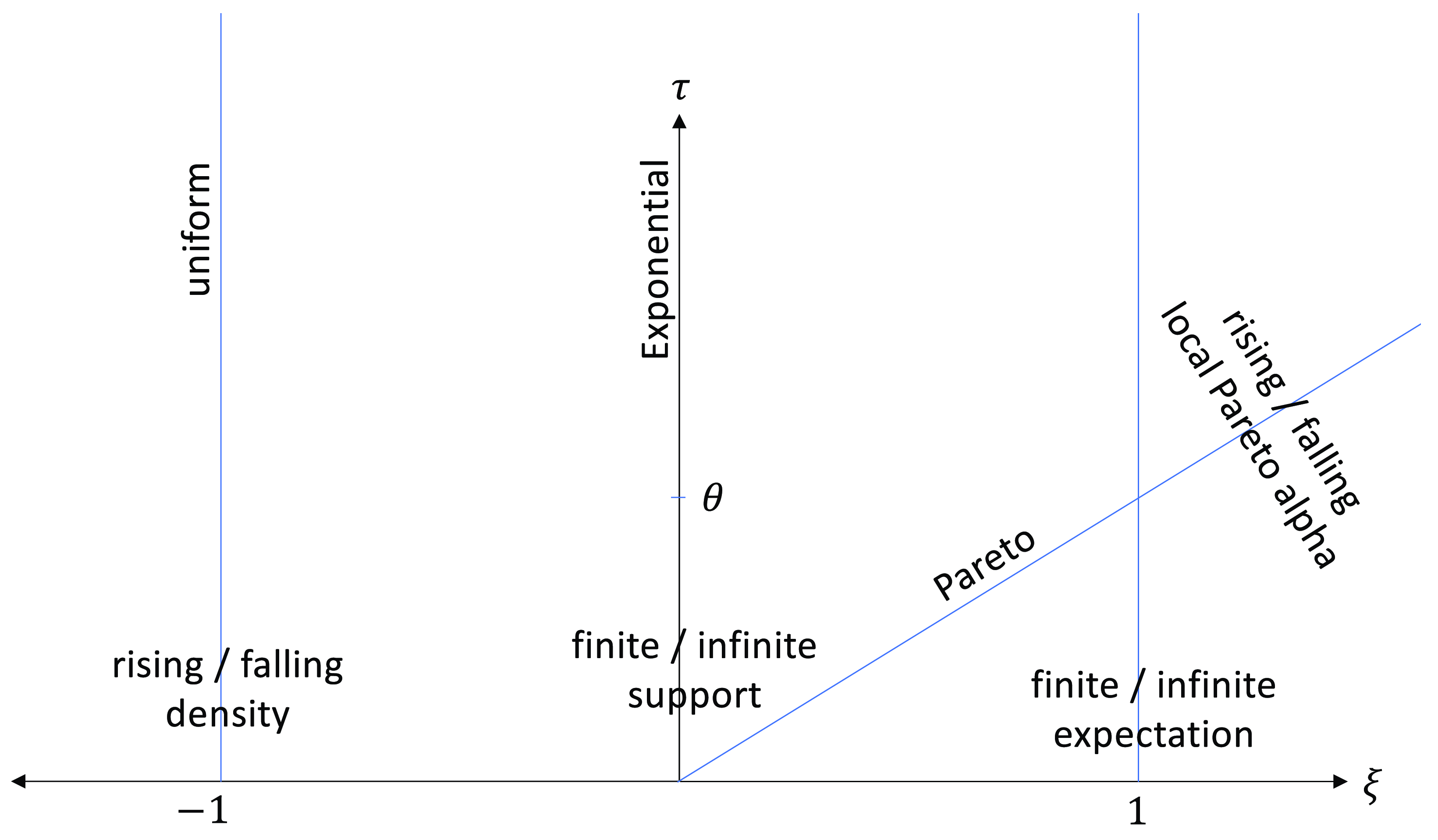
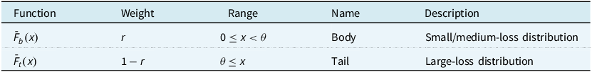
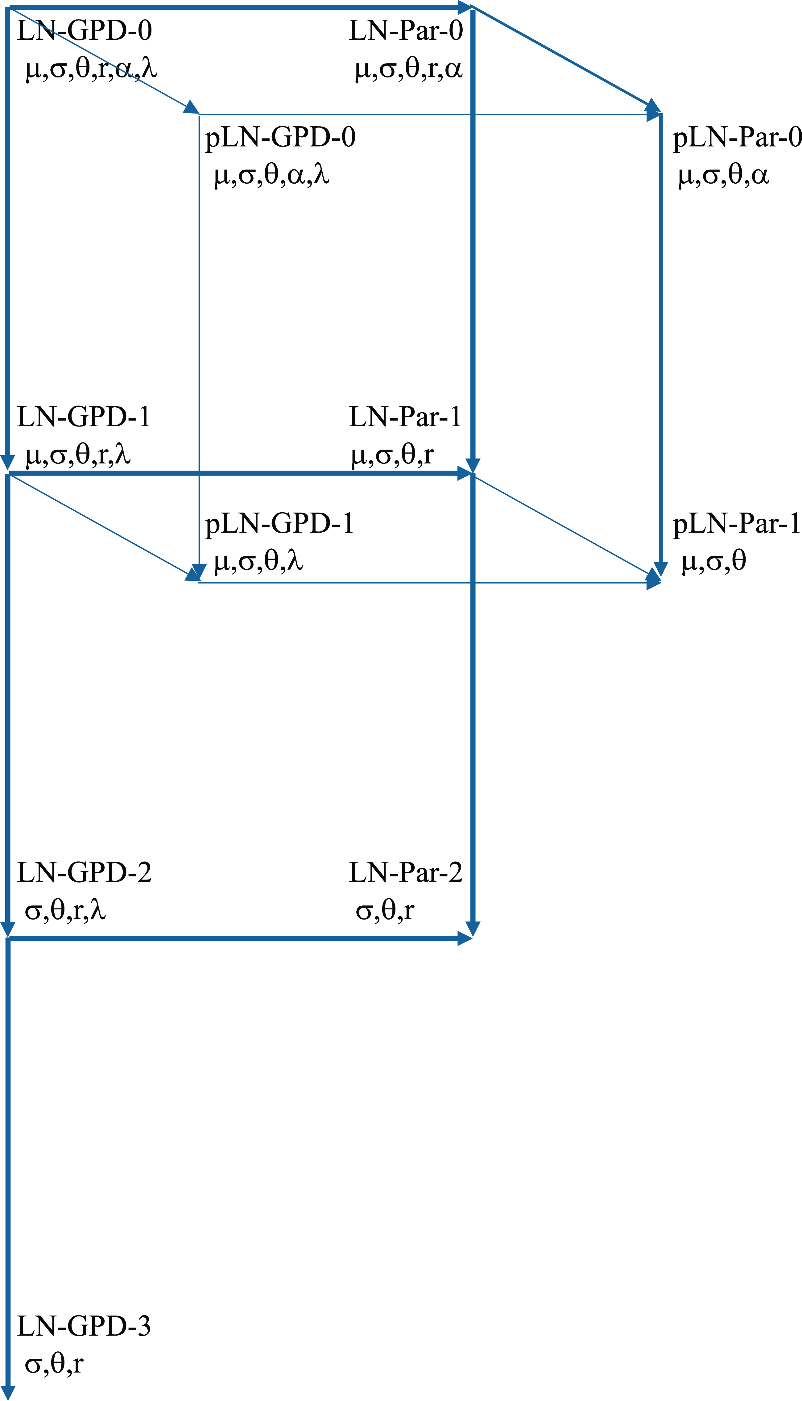
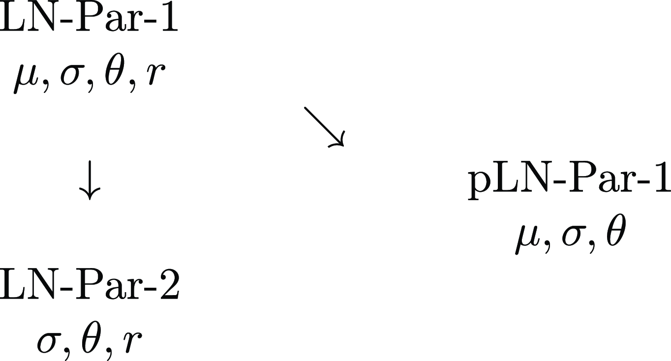
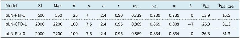
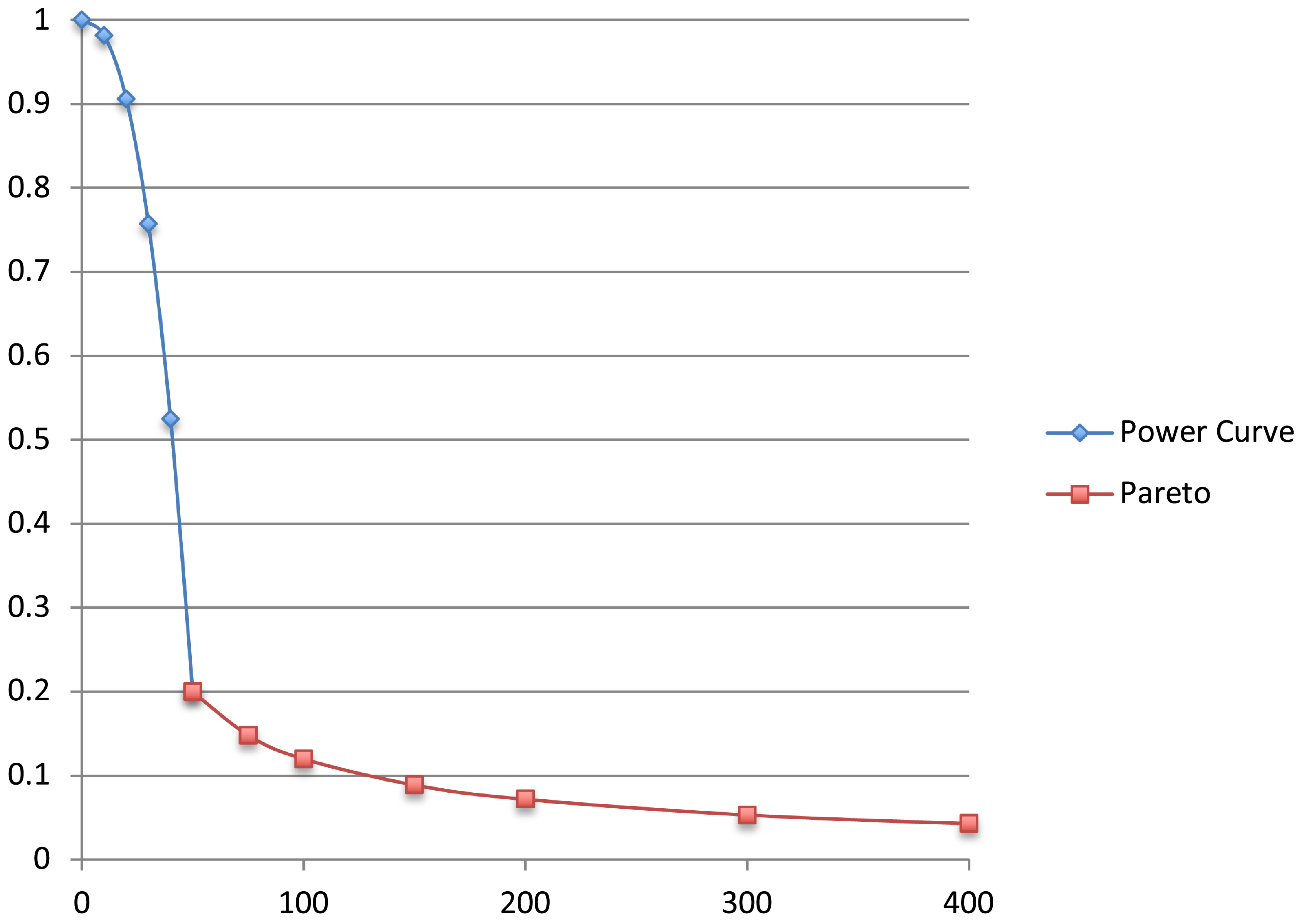
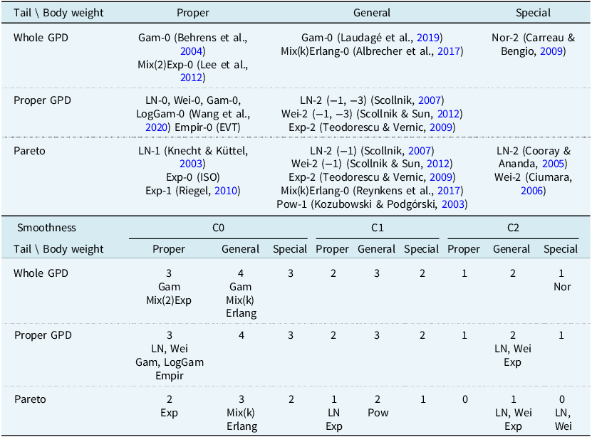


 Open access