





Introduction
Sub-annual glacier surface velocity changes are driven by variable rates of basal motion (Willis, Reference Willis1995, and references within). Basal motion often accounts for a large fraction ($\sim 50 - 100\percnt$ ) of glacier mass flux (Raymond, Reference Raymond1971; Truffer and others, Reference Truffer, Harrison and Echelmeyer2000; Harrison and others, Reference Harrison2004; Amundson and others, Reference Amundson, Truffer and Luthi2006; Morlighem and others, Reference Morlighem, Seroussi, Larour and Rignot2013; Ryser and others, Reference Ryser2014b; Doyle and others, Reference Doyle2018; Maier and others, Reference Maier, Humphrey, Harper and Meierbachtol2019) across a wide range of glaciologic settings (Maier and others, Reference Maier, Humphrey, Harper and Meierbachtol2019), from valley glaciers to the ice sheets. Basal motion is possible under the large temperate fractions of the Greenland ice sheet ($\sim 43\percnt$
 ) (MacGregor and others, Reference MacGregor2016) and Antarctica ($\sim 55\percnt$
 ) (Pattyn, Reference Pattyn2010), making its understanding important for predicting ice fluxes to the global ocean and thus, sea level rise. Basal motion also mediates mass change on valley glaciers, which disproportionately contribute to modern sea level rise (Meier and others, Reference Meier2007; Gardner and others, Reference Gardner2013; Zemp and others, Reference Zemp2019) and affect downstream water resources (O'Neel and others, Reference O'Neel, Hood, Arendt and Sass2014; Huss and Hock, Reference Huss and Hock2018; Pritchard, Reference Pritchard2019) and habitat quality (Hood and Scott, Reference Hood and Scott2008; Lydersen and others, Reference Lydersen2014; O'Neel and others, Reference O'Neel2015). Finally, as basal motion is the means by which glaciers erode their beds (Hallet, Reference Hallet1979; Iverson, Reference Iverson1991; Herman and others, Reference Herman2015; Koppes and others, Reference Koppes2015), its mechanics are critical for landscape evolution over geologic timescales.
Basal motion depends on gravitational driving stress (Weertman, Reference Weertman1957) and subglacial water pressure, with high subglacial water pressure (e.g., Iken and Bindschadler, Reference Iken and Bindschadler1986) or increasing en- and subglacial water storage (e.g., Bartholomaus and others, Reference Bartholomaus, Anderson and Anderson2008) corresponding to times of rapid basal motion. Basal motion occurs as slip at the ice-rock interface (Weertman, Reference Weertman1957; Lliboutry, Reference Lliboutry1968), slip at the ice-till interface, or by deformation within underlying till (Alley and other, Reference Alley, Blankenship, Bentley and Rooney1986; Truffer and others, Reference Truffer, Harrison and Echelmeyer2000; Kjær and others, Reference Kjær, Larsen, van der Meer, Ingólfsson, Krüger, Örn Benediktsson, Knudsen and Schomacker2006). Irrespective of the precise physical mechanism involved, as water pressure approaches the ice overburden pressure, basal traction declines and basal motion increases (Nienow and others, Reference Nienow2005).
Glacial basal motion exhibits seasonal change due to the annual evolution of glacier hydrology (Willis, Reference Willis1995; Fountain and Walder, Reference Fountain and Walder1998). Below, we outline a simplified conceptual model for the seasonal evolution of these systems that well describes the general behavior of many glaciers. In the cold season, water inputs to the glacier hydrologic system are negligible and basal water pressure (Rada and Schoof, Reference Rada and Schoof2018) and basal motion are relatively constant, although exceptions have been observed (e.g., Schoof and others, Reference Schoof, Rada, Wilson, Flowers and Haseloff2014). Surface melt begins in spring, and meltwater reaching the bed encounters a ‘distributed’ subglacial hydrologic system that is inefficient at transmitting water fluxes downglacier and thus experiences large changes in water pressure for a given water input. This results in the distributed system responding to meltwater inputs, which produces the commonly observed ‘spring speedup event’ (e.g., Mair and others, Reference Mair2003; Kessler and Anderson, Reference Kessler and Anderson2004; Colgan and others, Reference Colgan2012). This event is terminated by the establishment of ‘channelized’ subglacial drainage that is capable of transmitting large water fluxes, which decreases subglacial water pressure. Glacier basal motion typically reaches a minimum in late summer/early fall, when the drainage system has reached its maximum efficiency and meltwater inputs begin to decline. This system is thought to operate similarly on valley glaciers and ice sheets (e.g., Sole and others, Reference Sole2011), though the viability of maintaining channelized drainage under thick ice remains in question due to differing results in modeling work (Dow and others, Reference Dow, Kulessa, Rutt, Doyle and Hubbard2014) and observational studies (Chandler and others, Reference Chandler2013; Meierbachtol and others, Reference Meierbachtol, Harper and Humphrey2013).
This straight-forward conceptual model has several simplifications. Despite this picture of monotonic increase in drainage efficiency throughout the melt season, recent work shows that rapid switching back-and-forth between modes of subglacial drainage occurs during this transition (Rada and Schoof, Reference Rada and Schoof2018). Further, increasing evidence suggests decreasing areal extent of a third mode of ‘disconnected’ subglacial drainage (Iken and Truffer, Reference Iken and Truffer1997) may explain long-term (~ weeks-months) velocity decrease throughout the melt season (Andrews and others, Reference Andrews2014; Hoffman and others, Reference Hoffman2016; Rada and Schoof, Reference Rada and Schoof2018). In addition, direct measurements frequently document large variations in the magnitude and temporal behavior of subglacial water pressure over short horizontal spatial scales (< 20 m; Harper and others, Reference Harper, Humphrey, Pfeffer, Fudge and Neel2005; Rada and Schoof, Reference Rada and Schoof2018) and often exhibit a complicated, if any, link to surface velocity changes (Harper and others, Reference Harper, Humphrey, Pfeffer, Fudge and Neel2005, Reference Harper, Humphrey, Pfeffer and Lazar2007). Andrews and others (Reference Andrews2014), however, found that water pressures in moulins correspond well over large horizontal distances and are well correlated with diurnal velocity changes.
Here, we investigate stage on an ice-marginal lake to determine if it behaves similarly to the moulins of Andrews and others (Reference Andrews2014) and may provide a proxy for subglacial water pressure. Ice-marginal lakes have been studied extensively in the context of glacier lake outburst floods (e.g., Post and Mayo, Reference Post and Mayo1970; Clarke, Reference Clarke2003; Walder and others, Reference Walder2006; Sugiyama and others, Reference Sugiyama, Bauder, Weiss and Funk2007; Bartholomaus and others, Reference Bartholomaus, Anderson and Anderson2008; Riesen and others, Reference Riesen, Sugiyama and Funk2010; Carrivick and others, Reference Carrivick2017) and mathematical analysis of their complicated stage dynamics (e.g., Ng and Björnsson, Reference Ng and Björnsson2003; Kingslake, Reference Kingslake2015). However, the utility of ice-marginal lakes as a proxy for subglacial conditions has not been thoroughly researched.
The seasonal evolution of subglacial hydrology drives changes in the glacier force balance because greater stress-gradient coupling must compensate for decreases in basal traction (e.g., O'Neel and others, Reference O'Neel, Pfeffer, Krimmel and Meier2005; Price and others, Reference Price, Payne, Catania and Neumann2008; Ryser and others, Reference Ryser2014b). Several recent field studies have documented the importance of longitudinal stress transfer in controlling glacier ice speed. Ryser and others (Reference Ryser2014a) showed that horizontal stress transfer between time-variable ‘sticky patches’ (i.e., regions of high basal friction) and surrounding ‘slippery patches’ controlled the spatial pattern of ice motion over a portion of the Greenland ice-sheet ablation zone. On a smaller scale, Flowers and others (Reference Flowers, Jarosch, Belliveau and Fuhrman2016) showed high sensitivity of basal motion to water inputs at one part of a glacier drove surface speed variations at other stations which were less sensitive to local meltwater inputs. Relatively uniform increase in summer basal motion averaged over several weeks to several months have been observed on Kennicott Glacier (Armstrong and others, Reference Armstrong, Anderson, Allen and Rajaram2016) and a larger collection of south-central Alaska glaciers (Armstrong and others, Reference Armstrong, Anderson and Fahnestock2017). The uniformity of summer speedup over long distances may result from theoretically-expected increase in the longitudinal stress-gradient coupling length scale on slippery-bedded glaciers (Kamb and Echelmeyer, Reference Kamb and Echelmeyer1986) or from self-regulation of the rate of basal motion.
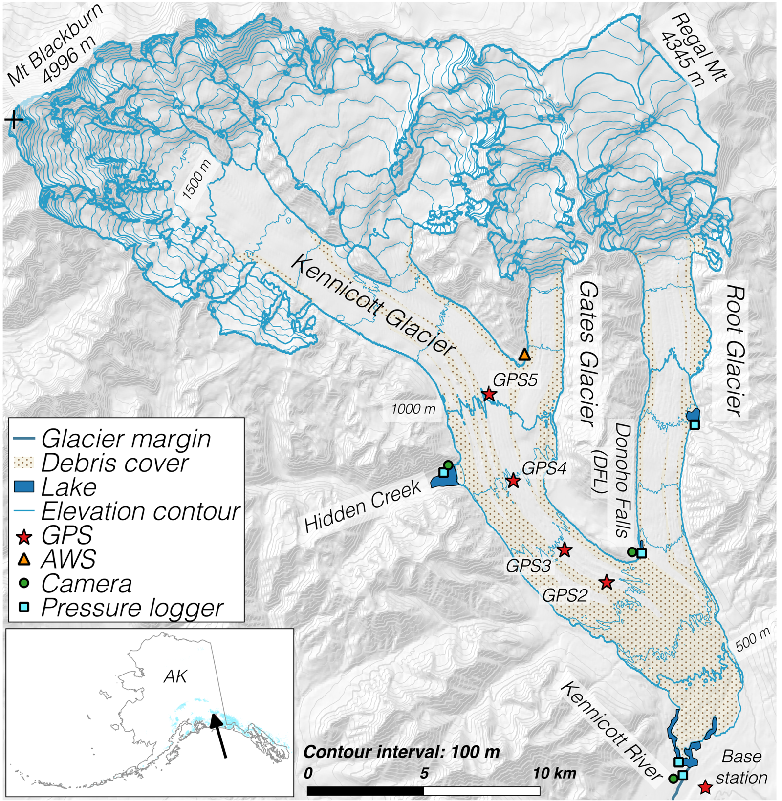
In this manuscript, we study the link between subglacial hydrology and glacier basal motion, and investigate how the seasonal evolution of basal motion affects bulk ice flow through a 10 km study reach. We accomplish this utilizing water level in an ice-marginal lake, meteorological data and short-term velocity variations on Kennicott Glacier, Alaska (Fig. 1), primarily over the 2012 spring–summer transition (DOYs 130–165). This period is a time when the glacier hydrologic system and its controls on glacier velocity are rapidly changing. The primary objectives of this manuscript are to: (1) document the complicated springtime progression of lake level on an ice-marginal lake and concurrent glacier velocity timeseries measured via on-glacier GPS; (2) investigate the temporal evolution of diurnal velocity fluctuations at a point in space; (3) show how these variations change the flow field over a ~ 10 km centerline profile; and (4) jointly analyze velocity and hydrometeorological data to probe the link between glacier hydrology and basal motion.
Map of field site and monitoring equipment. Symbols show equipment locations. Stars indicate on-glacier global position system (GPS) monuments. Circles and squares indicate timelapse cameras and pressure transducers, respectively. The triangle shows a National Park Service maintained automated weather station (AWS). Analyses in the current study primarily focus on the on-glacier GPS and the Donoho Falls Lake (DFL) stage record. Inset shows study location within the state of Alaska, indicated with an arrow. Glacierized area is shown in teal. Glacier outline is from the Randolph Glacier Inventory (RGI Consortium, 2017). Elevation data are extracted from the National Elevation Dataset and are shown with a 100 m contour interval. Stippled pattern represents supraglacial debris cover, mapped from a 2015 Landsat 8 image.
Methods
We investigate seasonal evolution of glacier velocity and whether ice-marginal lake hydrology may be used as a proxy for subglacial hydrologic conditions controlling velocity behavior. To accomplish this, by the end of this manuscript, we present several distinct types of time series: (1) time series of ice-marginal lake level (stage); (2) time series of glacier velocity along a ~10 km longitudinal GPS transect; and (3) time series of derived products, such as rates of change of ice-marginal stage and glacier velocity, lag times between velocity records at different stations and timing of daily maxima and minima. Here, we foreshadow our interpretation of these quantities to guide the reader's analysis of our results. We utilize ice-marginal lake stage and its rate of change (ROC) as rough proxies for regionally-averaged subglacial water pressure. We analyze changes in glacier acceleration and deceleration rates, as well as the timing of daily maxima as measures of the efficiency of the glacier hydrologic system. We investigate correlations between velocity records at different stations to assess the spatial uniformity of glacier flow. Below, we describe these methods in detail, as well as the study area at which we employ them.
Study area
Our investigation takes place on Kennicott Glacier in the Wrangell Mountains of Alaska (61.50° N, − 142.95° E; Fig. 1). Kennicott Glacier is 43 km long, temperate, land-terminating and has ice thickness exceeding 500 m (M. Truffer and J. Holt, unpublished data; Armstrong and others, Reference Armstrong, Anderson, Allen and Rajaram2016). Kennicott Glacier spans 4500 m of elevation from the 4996 m a.s.l. Mt Blackburn to the glacier's terminus at 490 m a.s.l. Kennicott Glacier has retreated by ~500 m from its Little Ice Age (LIA) maximum extent (Rickman and Rosenkrans, Reference Rickman and Rosenkrans1997) and has lost 0.43 m w.e. a−1 on average over 2000–2013 (Larsen and others, Reference Larsen2015). A growing proglacial lake lies between the terminus and LIA moraine, but the glacier lacks an active calving front. Approximately 19% (~ 70 km2) of Kennicott Glacier is debris-covered, with debris thickness upwards of 1 m (L. Anderson and others, in review). It is unknown whether the glacier bed is dominantly till-mantled or bare bedrock.
Previous studies on Kennicott Glacier have largely focused on the mechanics of its annual outburst flood (Anderson and others, Reference Anderson2003; Walder and others, Reference Walder2006), its link to basal motion (Anderson and others, Reference Anderson, Walder, Anderson, Trabant and Fountain2005; Bartholomaus and others, Reference Bartholomaus, Anderson and Anderson2008, Reference Bartholomaus, Anderson and Anderson2011) and hydrochemical analyses (Anderson and others, Reference Anderson2003). In this work, we do not focus on outburst flood processes, but instead investigate the ice-marginal Donoho Falls Lake (DFL) and seasonal glacier dynamics. DFL is located at the tributary junction of Kennicott Glacier and the smaller Root Glacier, ~ 9 km up-valley of the glacier terminus and ~ 8 km down-valley of Hidden Creek Lake (Fig. 1), the source of the annual outburst flood. DFL is impounded by Root Glacier, though it is sensitive to Kennicott subglacial processes, as evidenced by its brief ~ 0.5 × 10⁶ m3 filling during the Hidden Creek Lake outburst event, which drains beneath Kennicott Glacier. DFL is at a similar up-glacier distance to our lowest GPS station. The lake is located at a glacier surface elevation of ~ 680 m, within ~ 110 m elevation of our two lowest on-glacier GPS stations.
GPS installation and maintenance
We maintained on-glacier GPS monuments in 2012–2014, though only present spring–summer 2012 results here due to power loss and data quality issues in the subsequent seasons. Similar data collected in 2006 data are published in Bartholomaus and others (Reference Bartholomaus, Anderson and Anderson2008, Reference Bartholomaus, Anderson and Anderson2011). We anchor the GPS antennae to the glacier following the methods of Anderson and others (Reference Anderson2004), described in greater detail in Supplementary Material. We installed four GPS monuments along the approximate glacier centerline every 2–3 km along a 10 km reach ranging from 750 to 1020 m a.s.l (Fig. 1). At our most up-glacier and down-glacier GPS monuments, we measure air temperature with a thermistor housed in a radiation shield and the rate of surface melt using a look-down sonic ranger controlled by and recorded on an open-source Northern Widget data logger (Wickert, Reference Wickert2014; Wickert and others, Reference Wickert, Sandell, Schulz and Ng2019). We periodically re-drill the stations throughout the ablation season to ensure the antennae remain near level. GPS equipment was provided by unavco. GPS station numbers increase moving up-glacier, such that high numbers denote high elevation (Fig. 1).
GPS processing for velocity timeseries
We convert GPS data using unavco-standard software, and then differentially process on-glacier stations relative to a static base station (~ 10 − 20 km baseline) using the track module within gamit-globk (Herring and others, Reference Herring, King and McClusky2006) software with default processing parameters.
We identify and manually correct position change due to GPS station maintenance. Data with > 0.02 m reported horizontal position uncertainty are removed from this analysis. We manually remove additional low-quality data, assessed largely by abrupt, non-physical variation from ‘background’ behavior. Position change during data gaps due to power loss is estimated by linear interpolation, which allows us to determine the average rate of position change over the gap. We then rotate the data into a flow-oriented coordinate system (Supplementary Material).
The resulting position data have high-frequency noise that render accurate velocity estimation impossible without further processing. We up-sample the data (i.e., coarsen its temporal resolution) by decimating the 30 s positions to 15 min positions and then smooth the data using a bisquare (quartic) kernel weighted mean. We use ± 3.5 h for the width of the bisquare kernel for smoothing horizontal positions, which we found minimizes noise while retaining physically-meaningful diurnal velocity fluctuations. We smooth the vertical coordinate using a ± 12 h kernel width, as the vertical coordinate has higher position uncertainty. Finally, we calculate the velocity by differencing the smoothed 15 min positions.
Investigating changes in the diurnal velocity and stage fluctuations
The shape of diurnal velocity fluctuations conveys information about the efficiency with which meltwater is routed to and evacuated from the glacier bed, as well as the sensitivity of basal motion to water inputs. We create diurnally stacked velocity time series by analyzing velocity data as a function of time of day, rather than time of year. We identify diurnal extrema (i.e., maxima and minima) in the on-glacier velocity records, using the matlab function peakdet with delta = 0.01 m d−1. We then analyze seasonal changes in the time at which diurnal velocity extrema occur by fitting a linear regression to these data using polyfit and test for statistical significance of these trends using regress. We perform an identical analysis to assess the magnitude and timing of DFL stage, stage ROC and air temperature.
We investigate the peakedness of diurnal velocity fluctuations by calculating the rate of acceleration into and deceleration from velocity maxima. To do this, we first isolate days with large diurnal velocity ranges (Δu), here defined as Δu ≥ 0.125 m d−1. We center each day's velocity record about its time of peak velocity. We then standardize the records by calculating the velocity change from the day's peak velocity, where zero corresponds to the peak velocity and more negative values denote slower speeds. We then use 4 h of data (16 velocity data points) to construct linear fits of the progression of velocity up to and down from the velocity peak. The slope of these linear fits describes the glacier acceleration rate, where a positive slope indicates increasing velocity.
Assessing inter-station velocity lags
The spatiotemporal pattern of variations in glacier velocity provides clues into the controls on glacier speed. We assess the uniformity of velocity variations (or lack thereof) by cross-correlating velocity records at different GPS stations. We iteratively calculate the correlation between velocity records at GPS5 and the down-glacier stations, with varying lags to the GPS5 time series. The magnitude of the peak correlation between stations and the tightness of this peak provides a quantitative metric to describe uniformity of glacier velocity behavior across the study reach. We use 3 d of data for each calculation, incorporating 288 data points for each correlation if there are no data gaps during the correlation period. We only compute correlations for points in time in which $\leq 40\percnt$ of the 3 d window is missing data, meaning there are always ≥ 173 valid data points. Using all data points within this 3 d window means that we are not correlating timing of solely velocity maxima, but rather the entire diurnal velocity curve, including maxima, minima and points in between. We hold the down-glacier station constant in time, and shift the velocity record from the up-glacier station in time. We iteratively shift the up-glacier station from − 6 to + 18 h by 15 min increments. A negative lag implies the up-glacier station leads in its diurnal velocity cycle. The time lag with the highest correlation over a 3 d span is chosen as the best-fitting lag time. We repeat this analysis with each station pair over our observation period to produce a record of inter-station lag time of peak velocities over the course of the melt season.
Ice-marginal hydrology and melt timing
We deployed Solinst LevelLogger (Model 3001) pressure transducers on ice-marginal lakes as well as the proglacial lake and Kennicott River. We convert pressure to water height using an assumed water density of 1000 kg m−3 and neglecting barometric pressure variations. These assumptions introduce error into our analysis that is small relative to stage fluctuations. The transducers are accurate to 0.05% of the full range of the instrument's measurement capability, corresponding water height uncertainty of these sensors is therefore ± 5 and ± 1.5 cm depending on the model (with either 100 or 30 m range). The sensors also measure temperature. Data are recorded every 15 min.
In addition to pressure transducers, we deployed Moultrie timelapse cameras to monitor lake levels. These cameras capture an image every hour and allow lake level reconstruction when the water level dropped below the pressure transducers. We calibrate time lapse imagery using the mid-summer outburst flood record, at which time we have concurrent pressure transducer data and images as the flood wave completely fills to the once-empty basin. We digitize the lake levels associated with ~ 10 m changes in the pressure transducer record to establish a calibrated reference image (Fig. 2). We have pressure transducer data at this time because we moved the instrument to the lowest portion of the basin after the lake drained in early summer. We then manually identify daily lake stage maxima and minima from timelapse imagery and estimate the associated lake stage using the reference photo (Fig. 2). While digitizing, we withhold the spring pressure transducer record where there is overlap. Comparing these two datasets during times of overlap provides a measure of uncertainty in the digitizing process, which we found to be < 3 m in magnitude and < 1 h in timing (Fig. 3a). We do not perform quantitative analyses using stage data from digitized photos, but instead employ it to gain rough insight during times the lake level was below the pressure transducer.
Timelapse camera images of Donoho Fall Lake (DFL) on (a) 28 May 2012, and (b) 31 May 2012. Red lines show apparent lake extent associated with the pressure transducer stages used for photo digitizing. The heavy orange line shows the near vertical ice wall used as a reference to establish lake stage. Thin orange lines show unchanging features used for image coregistration. Relationships between lake height (stage) and (c) volume and (d) sensitivity of height change to volume change when DFL geometry is approximated as a right triangular pyramid, as shown in the inset in (d). Symbol meanings and values shown in the inset are defined in the text.

Time series of 2012 hydrology and glacier motion. (a) Donoho Lake stage (dark blue for pressure transducer, light blue with circles for digitized photos) and air temperature (red), (b) on-glacier GPS longitudinal velocity, (c) longitudinal strain rate between several station combinations and (d) relative elevation of the GPS antenna. Dashed lines in (c-d) indicate average values during times of power failure. The black lines in (d) show the approximate range of uplift expected from vertical strain using the parameters shown in Table 1. The thin and heavier black lines show uplift using the parameters that produce minimal and ‘realistic’ bed separation, respectively.

Estimates of components contributing to ice surface uplift. The top rows show parameter choices that minimize the contribution of bed separation to uplift. The bottom rows show parameter choices closer to the best known values for Kennicott Glacier during the study period. Ice thickness (H), longitudinal strain rate (u/x), horizontal velocity (u) and glacier surface slope (α) values are shown for each case

aAll vertical velocities (w) are reported in units of cm d−1.
bUplift due to bed separation w sep is calculated as w sep = w tot − w strain − w slope − w tilt. The percent uplift due to bed separation is calculated as w sep/(w tot − w slope).
We use air temperature above 0°C as a proxy for glacier melt rather than employing a positive degree day melt model (Hock, Reference Hock2005). This simple approach is sufficient for our purposes because we only seek to find the timing of peak diurnal melt, and do not estimate the total amount of melt produced.
Estimating Donoho Falls Lake geometry
To aid in interpretation of the DFL stage record, we construct a DFL stage–volume relation by approximating the basin's geometry as a right triangular pyramid (Fig. 2d inset). Lake volume (V) can therefore be related to height (h) by,

where θ is the average slope of the basin along the lake's short planview axis, and Ω is the average slope along the half-width in the lake's long planview axis (Fig. 2d inset). From field survey and analysis of satellite imagery, we find θ = 0.32rad = 18° and Ω = 0.27 rad = 15°. The ROC of volume as a function of lake height (∂V/∂h) is then calculated as,

These equations are plotted in Figures 2c, d. We later use these relationships to develop a conceptual model to guide interpretation of the DFL stage record.
Results
Spring stage variations on Donoho Falls Lake
Each spring, we observe a complicated sequence of filling and draining of the ice-marginal DFL (Figs 1, 3a, and S1; Supplemental Video). In 2013, we capture our most complete record of spring DFL stage and find the initial filling on DOY 126, which occurs shortly after the onset of > 0°C air temperatures (Fig. S1). Spring 2013 was relatively late and cool and we observe a 31 m DFL stage increase that occurs relatively steadily over DOYs 126–134, corresponding to an average filling rate of 3.7 m d−1. After this point in time, the filling rate slows to 1.1 m d−1 over DOYs 134–141. Diurnal stage fluctuations then appear and the average filling rate further slows to 0.50 m d−1. Coincident with a sudden increase in air temperature (DOY ~ 145; Fig. 3a), DFL stage drops by 14.8 m over 2.3 d. This drop is followed by a ~ 5 day long standstill in mean stage with ~ 4.5 m diurnal stage fluctuations (peak-trough amplitude). This is followed by a ~ 25 m stage drop with ~ 10 m amplitude diurnal fluctuations. We then observe a ~ 31.5 m stage rise over ~ 2.5 d, coincident with another period of high air temperature (DOY ~ 157; Fig. 3a). After rapid lake drainage initiating late on DOY 161, we observe two short-lived refilling events that coincide with warm periods before the basin drains for the remainder of the spring. We discuss the timing of DFL stage extrema and its evolution in a later section. The 2012 and 2014 DFL stage time series exhibit similar dynamics to those described above (Figs 3a and S1). Spring 2014 was warmer than the preceding 2 years and the final lake drainage occurred earlier in the melt season (Fig. S1).
GPS-derived velocity and strain rate time series
We observe glacier velocity variations occurring over two distinct timescales: (1) diurnal fluctuations of varying amplitude but consistent presence throughout the study period; and (2) spring speedup events initiating around DOY 130–140 and lasting until DOY 150–170 (Figs 3 and S2). In the current study, we focus on the evolution of glacier velocity between DOYs 130–200 in 2012 due to high-quality velocity records and overlap between velocity and DFL stage at this time. The Hidden Creek Lake outburst flood occurred on DOY 201 in 2012, so jökulhlaup dynamics do not complicate the analysis of this earlier period. The first portion (DOY 130–165) of this period coincides with the stage variations on DFL, and allows us to investigate the link between the glacier hydrologic system and velocity change during the spring speedup and transition into summer. We include the later velocity data primarily for the analysis of diurnal velocity behavior and links between velocity at different parts of the glacier.
In 2012, the spring speedup at the down-glacier GPS2 and GPS3 stations begins abruptly on DOY 141, as evidenced by the onset of large amplitude diurnal velocity fluctuations and an increase in mean velocity, although there is some suggestion of a slow speedup beginning DOY 137 (Fig. 3b). This possible onset of speedup on DOY 137 closely coincides with the initiation of > 0°C air temperatures (Fig. 3a). This speedup at down-glacier stations is accompanied by acceleration at the up-glacier GPS4 and GPS5 stations, with much smaller or negligible diurnal velocity fluctuations (Fig. 3b). The onset of high amplitude diurnal velocity fluctuations does not begin at GPS5 until DOY 158, lagging the down-glacier stations by 11 d. We find large amplitude diurnal velocity fluctuations at GPS3 throughout the period of record and more muted diurnal cycles at GPS5 (Fig. S2b).
Longitudinal strain rates ($\dot \epsilon _{xx}$ ) are generally compressive through the study reach, with median $\dot \epsilon _{xx}$
 ranging from − 2.4 × 10⁻⁵ to − 2.7 × 10⁻⁵ d−1 depending on chosen stations (Figs 3c and S2c). We observe significant variation about the median value over diurnal and multi-day timescales due to varied phasing of velocity cycles between stations. The onset of the spring speedup at the down-glacier stations causes a reduction in the mean magnitude of compressive strain rate to $\dot \epsilon _{xx} \approx -1.0 \times 10^{-5}$
 d−1. This period is accompanied by short-lived excursions to extensional strain rates ($\dot \epsilon _{xx} = 2.2 \times 10^{-5}$
 d−1). The onset of the spring speedup at GPS5 brings $\dot \epsilon _{xx}$
 back to a value similar to its pre-speedup state. The increasing synchroneity between station velocity change later in the melt season reduces the magnitude of diurnal variations in $\dot \epsilon _{xx}$
 (Fig. 3c).
The speedup is accompanied by a two-phased ice uplift at all stations. The uplift amplitude decreases up-glacier (Fig. 3d). The onset of uplift appears to propagate as a wave, with GPS5 lagging GPS2 by 5.5 d, which corresponds to a wave speed of 1.87 km d−1. GPS2 is uplifted 0.32 m over 6.9 d, an uplift rate of ~ 0.045 m d−1. The uplift rate then slows to ~ 0.03 m d−1 over DOYs 148.3–162.7. In 2012, uplift at the down-glacier GPS2-3 is accompanied by the onset of pronounced diurnal velocity fluctuations, while at the up-glacier GPS5, the onset of velocity diurnals lags the initiation of uplift by at least 8 d.
The 2012 record is characterized by monotonic uplift at all stations throughout the spring–summer transition (Fig. 3d), with lower stations experiencing greater total uplift. This pattern does not repeat each year, however, with surface uplift at GPS3-5 in 2014 occurring quickly (8 cm d−1 sustained for 2.3 d), remaining relatively stable for 10 d, and then decaying to zero in a quasi-exponential fashion (Fig. S2d).
We compute rough estimates of processes that can result in glacier surface uplift to aid interpretation of the uplift time series. The GPS antenna do not lower with ablation, so their elevation change reflects the sum of vertical strain, horizontal motion down a sloped surface and changing volume of subglacial cavities that cause changing ice-bed separation (e.g., Anderson and others, Reference Anderson2004). Mathematically, this may be stated,

where w tot is the measured total GPS antenna vertical velocity (taken to be positive upwards), w strain is the vertical velocity due to vertical strain, w slope is the vertical velocity due to ice surface parallel motion, and w sep is the vertical velocity due to changing bed separation.
The vertical velocity arising from longitudinal compression can be estimated from

where H is the ice thickness, and ∂u/∂x is the longitudinal strain rate. This equation is approximately true when cross-glacier velocity is near zero and the longitudinal strain rate at the surface closely reflects the column-averaged longitudinal strain rate. We compute w sep as the remaining vertical velocity after accounting for the other contributors to surface uplift. We compute a range of possible vertical velocities due to hydraulically-induced bed separation by using values that minimize bed separation as well as values more typical to our study period (Table 1). Strain rates, horizontal and vertical velocities are estimated from Figure 3. The 3% ice surface slope used for both scenarios and range of ice thickness are reported in Armstrong and others (Reference Armstrong, Anderson, Allen and Rajaram2016). We do not use time variable strain rates for this calculation because we only seek a rough estimate of hydraulically-induced surface uplift, and not a detailed time series of bed separation, which would be subject to greater uncertainty. Depending on whether we consider conservative parameter values (i.e., ones that minimize bed separation) or best-guess values (Table 1), we estimate that hydraulically-induced bed separation is responsible for $\sim 60 - 80\percnt$ of the observed surface uplift.
Evolving diurnal velocity behavior at a single GPS station
The character of diurnal velocity fluctuations at a single point on the glacier surface provides information about the transmission of meltwater through the glacier hydrologic system and the glacier's velocity sensitivity to that water flux. The diurnal range of glacier velocity does not show systematic variation throughout the DOY 140–200 period (Figs 4a, b). However, it does appear that the manner in which glacier velocity approaches and leaves its diurnal peak evolves throughout the season. Diurnal maxima become shorter-lived events that are more quickly approached and more rapidly left, as shown by the progressive tightening of the standardized diurnal velocity curves in Figure 4b. Linear fits to the velocity time series on either side of the diurnal maximum, which show the glacier's acceleration and deceleration, become progressively more rapid throughout DOYs 140–180 (Fig. 4c). This indicates velocity maxima are approached and left more rapidly throughout the transition from spring into summer. Rates of acceleration are very similar (although opposite in sign) to rates of deceleration, resulting in a diurnal velocity curve that is symmetric about its maximum.
Diurnally stacked velocity records and time series of diurnal acceleration at GPS3. (a) Velocity as a function of time of day over DOYs 135–180 in 2012. Circles indicate diurnal velocity maxima. The same colorbar applies for (a–c), with warm colors showing days later in the year. Days with a diurnal velocity range (Δu < 0.125 m d−1) are shown as gray lines in (a, b). (b) Change in velocity as a function of time since peak velocity. Negative velocity indicates speeds less than the maximum daily velocity. (c) Time series of the rate of acceleration (circles) and deceleration (x's) from peak velocity. These records show diurnal peaks occur progressively earlier in the day, with faster acceleration into and deceleration from these peaks as the season progresses.

Evolving relationship between station velocities
We analyze time lags between GPS stations to determine the spatial and temporal coherence of diurnal glacier velocity fluctuations throughout our study reach. Time lags (or lack thereof) between different velocity records provide information about hydrologic routing from glacier surface to bed, and how it varies across the study area. We note that our analysis utilizes all velocity data within a 3 d window, so the inter-station correlation indicates similarity in the entire diurnal velocity cycle, including the timing and relative magnitude of diurnal velocity maxima, minima and the points in between.
As expected, regions closer together experience more similar velocity behavior, with shorter inter-station time lags between velocity maxima throughout the melt season (Fig. 5). In the early season (~ DOY 146), the up-glacier GPS5 lags the down-glacier stations by 0.75, 5 and 7 h (Fig. 5b), with larger lags at stations further down-glacier. The respective stations are 3.94, 7.78 and 10.27 km down-glacier from GPS5. Later in the summer, the timing of peak velocity becomes more similar (Figs 5d, e); in mid-summer (~ DOY 175), GPS5 lags by only 0.15, 1.00 and 1.25 h, respectively. Thus, in the early season, diurnal velocity fluctuations (e.g., timing of velocity maxima and minima) propagate up-glacier, with down-glacier stations speeding up earlier; in mid-summer, all points along the study reach begin their diurnal speedup at approximately the same time. In addition to more similar timing of the diurnal velocity cycle (i.e, shorter inter-station lags), we also find the maximum correlation value between 3 d-windowed station velocity records increases through the course of the melt season (Figs 5b, d). Taken together, the decreasing inter-station lags and increasing correlation indicate that glacier velocity becomes more homogeneous throughout our study reach as the season progresses, both in terms of timing and magnitude of diurnal velocity extrema.
Illustration of computation of lag time in the diurnal velocity cycle at GPS5 relative to the down-glacier stations, as well as how this lag changes over time. (a, c) show velocity time series centered on DOY 146 (May 25) and DOY 175 (June 23), respectively. (b, d) show correlation coefficients when data are iteratively lagged by varied amounts, with the inter-station-lag time chosen as the hour offset that produces maximum correlation between 3 d windowed velocity records. (e) Time series of lag times that maximize correlation between GPS5 and the down-glacier stations. Correlation maxima indicate the time lag at which GPS5 most closely resembles the velocity behavior of the down-glacier station. Positive lags indicate that GPS5 velocity peaks and troughs occur after the down-glacier station. Locations shown in Fig. 1.

Evolving links between GPS stations are apparent when the velocity at one station is plotted against another (Fig. 6) in a phase diagram. At the down-glacier stations GPS2 and GPS3, which are separated by 2.49 km, we find high velocity covariance throughout the spring period of record (DOYs 130–165; Fig. 6a). Plotting along the 1:1 line in Figure 6 indicates stations recording similar velocity time series. Figure 6a exhibits counter-clockwise hysteresis, indicating that the down-glacier GPS2 velocity increases precede those at the further up-glacier GPS3. The width of the hysteresis loops indicates the magnitude of temporal lag between stations; thus, GPS2 and GPS3 experience similar peak diurnal velocity timing throughout the record, indicated by the narrow hysteresis loops. Comparing GPS3 and up-glacier GPS5, however (Fig. 6b), we find an evolving relationship. Both stations experience similar multi-day speedup over DOYs 130–145, shown by early-season drift along the 1:1 line. Around DOY 145, high amplitude diurnal velocity fluctuations initiate at down-glacier GPS3 with no response at GPS5, indicated by horizontal lines in Figure 6b. After this point in time, the spring speedup passes GPS3, indicated by leftward drift, and around DOY 155, high amplitude diurnal oscillations occur at both stations. The relatively wide counter-clockwise hysteresis loops at this time indicate that the timing of peak velocity at GPS5 lags behind the down-glacier GPS3 by several hours, as shown in Figure 5e.
Evolving link between glacier velocity at different points. (a) Down-glacier stations GPS2 and GPS3. (b) Down-glacier GPS3 and up-glacier GPS5. Points are colored by time of year. Black dashed line shows 1:1. Locations shown in Figure 1.

Evolution of stage, temperature and velocity extrema timing
In general, the timing of maxima in air temperature and DFL stage ROC occur in the afternoon between 14:30 and 18:45 (Table 2 and Fig. 3). DFL stage maxima occur late in the day, often between 19:45 and 01:30. Glacier velocity shows a wide range of peak timing, varying between 16:20 and 23:20, and exhibits a significant linear time trend (p = 0.02) with peak velocity occurring about 20 min earlier each day as the season progresses from DOY 135 to DOY 165. In the early season, the timing of glacier velocity maxima generally coincides with that of DFL stage maxima, but later velocity maxima timing evolves to more closely coincide with maxima in stage ROC. Timing of stage ROC is tightly clustered (16:30–18:20) and exhibits a statistically significant trend (p = 0.07) toward earlier peaks, although this trend is weaker, changing by only ~6 min per day. Significant variability surrounds these long-term trends, with ~20% of variability explained by a linear fit (i.e., r 2 ≈ 0.2; Table 2 and Fig. 7). We note that the maxima occurring at 10:00 are an artifact of data processing on days where the quantity analyzed steadily declined, such that the point at which a new day was defined (10:00 in this case) was classified as the day's maximum.
Time series of the hour at which maxima (top) and minima (bottom) occur in Donoho Falls Lake stage, stage rate of change (ROC), on-glacier velocity and air temperature. Heavy lines show trends significant at the p ≤ 0.1 level and thin lines are not statistically significant. Marker size indicates the relative magnitude of that variable, where large symbols indicate high stage, rapid stage change, fast glacier motion and warm temperature for their respective variables. The interquartile ranges (IQR) of extrema timing are shown to the right of each plot with corresponding line colors. Stage IQR is not shown due to its high variability.

Statistics of extrema (i.e., minima and maxima) timing of Donoho Falls Lake stage, stage rate of change (ROC), on-glacier velocity and air temperature at an ice-marginal weather station. The first three columns indicate the 25th, 50th (median) and 75th percentile time at which extrema occurred, where 0 = midnight local time and 12 = noon local time. Hours greater than 24 indicate maxima that occur after midnight. Fractional hours indicate minutes, where 14.5 = 14 : 30. The fourth column shows the magnitude of linear trends in extrema timing in units of minutes per day, where negative trends indicate extrema occurring earlier in the day later in the year. The rightmost columns show the variance explained by the linear trend (r 2) and its statistical significance (p). Significant trends at the p ≤ 0.1 level are bolded

The timing of minima in air temperature, DFL stage ROC and glacier velocity occur in the morning between 04:30 and 09:45 (Table 2 and Fig. 7). Glacier velocity shows the tightest clustering of minima timing, with 50% of minima occurring between 05:00 and 07:30. The velocity minima generally correspond with, although slightly precede, stage ROC minima, which generally occur between 07:00 and 9:45. Stage minima occur in the afternoon and generally correspond, although slightly precede, maxima in stage ROC. Timing of velocity minima also exhibits a statistically significant trend (p = 0.01) with the day's slowest speed on average occurring ~ 20 min earlier each day, very similar to the shift in timing of velocity maxima. Timing of velocity minima generally corresponds with, although slightly precedes, minima in stage ROC and air temperature, neither of which exhibit significant trends.
Link between Donoho Falls Lake stage and glacier velocity
In previous sections, we characterized the DFL stage history, glacier horizontal displacement and vertical uplift time series, the progression of diurnal velocity behavior at a single point on the glacier, as well as the evolution of links between glacier velocity at different points. In this section, we now probe the relationship between glacier velocity and DFL stage during spring.
We find somewhat complicated, although discernible, relationship between the ROC of DFL stage and glacier speed. There is less evidence for a link between DFL stage and glacier velocity. As we describe above, this suggests limits to the transfer rate of water between DFL and the subglacial environment, and may indicate that stage ROC is a better proxy for subglacial water pressure than stage itself. At the scale of the entire study period, there appears to be general links between the speeds of the down-glacier stations GPS2 and GPS3 and DFL stage (Fig. 3). It should be noted that DFL is impounded by Root Glacier, not Kennicott Glacier, and there is a small peninsula of land separating DFL from the GPS sites. However, the lower GPS sites are at approximately the same up-glacier distance and elevation as DFL, which makes it plausible that the subglacial hydrologic systems in these two places will have evolved to similar states. GPS2 and GPS3 are located 2.0 and 3.4 km on a straight line from DFL, respectively, and are 0.91 and 3.50 km up-glacier from a line drawn perpendicular to glacier flow at the location of DFL (Fig. 1).
An example of the general link between velocity and DFL stage can be seen with the onset of the 2012 spring speedup event that occurs around DOY 138 at GPS2 and GPS3 coinciding with a 10 m amplitude DFL stage increase over the course of 4 d. The up-glacier GPS4 and GPS5 speedup began late on DOY 141, coincident with broad peak DFL stage (Figs 3a, b). However, there is no clear relationship between concurrent DFL stage and glacier velocity (Figs 8a, c), and DFL stage extrema lag velocity extrema by several hours for much of the study period (Table 2).
Phase diagrams of GPS3 velocity and Donoho Falls Lake (DFL) stage. Glacier velocity as a function of DFL stage (a) and stage rate of change (b). Glacier velocity above the day's minimum velocity as a function of stage (c) and stage rate of change (d). There is no clear relationship between either velocity or velocity change and DFL stage. However, some correspondence between DFL stage rate of change and glacier velocity is apparent.

DFL stage ROC appears to be a better predictor of the timing of glacier velocity maxima. High stage ROC shows some correspondence with high glacier velocity (Fig. 8b). Despite this general correspondence, significant scatter exists about this trend and one relationship does not exist across all times; a wide range glacier velocity is found at the same DFL stage ROC. Standardizing the velocity data by subtracting that day's minimum speed produces a stronger relationship (Fig. 8d), in which high rates of change correspond with velocities on the higher end of the diurnal range, although significant scatter in the data remain. We also find general agreement in the timing of maxima of the rate of infilling of DFL and GPS3 velocity, particularly in the later portion of the study period (Figs 7 and S3c and f).
We find stronger agreement between stage ROC and glacier velocity when considering only daily maxima for these quantities. There exists a statistically significant direct relationship (p = 0.003 utilizing all data points; p = 0.028 excluding the highest value data point) between peak daily stage ROC and peak daily glacier velocity (Fig. 9). The correlation between these variables indicates that time lags on the order of hours may exist between DFL stage ROC and glacier velocity, but that the two covary when analyzed with only daily time resolution.
Maximum daily glacier velocity as a function of the same day's maximum Donoho Falls Lake stage rate of change. Symbols are colored by the day of year to which they correspond. The dotted pink (dashed red) line shows the linear best fit to the data with (without) the point at ~ (0.3, 0.6), with associated statistical descriptors. Negative rate of change indicates days in which the lake continually drained.

Discussion
Below, we estimate the contributors to the DFL water balance, interpret the DFL stage record in the context of the evolution of subglacial hydrology, examine the time evolution of diurnal velocity cycles, and probe links between DFL stage and glacier basal motion. We then highlight how time variations in basal motion impact bulk glacier dynamics.
Assessing Donoho Falls Lake water balance
Each spring, DFL exhibits a complicated time series with > 50 m fill-and-drain sequences (Figs 3a and S1) before emptying for the remainder of the summer. Interpreting the physical significance of these stage variations requires a conceptual model for the dominant controls on lake level to ascertain the relative importance of subglacial and non-subglacial water sources. The evolution of subglacial hydrology could affect DFL stage either by limiting the rate of lake water outflow or by pressurized subglacial water that is ‘backed up’ and forced into the DFL basin. If large-scale stage changes are largely driven by subglacial dynamics, either of these mechanisms would indicate an ‘overwhelmed’ subglacial hydrologic system that is incapable of efficiently transmitting incoming meltwater.
We construct a rough water balance for the lake, in which lake stage is set by the balance of its water inputs and outputs. We estimate the importance of subglacial water on the DFL stage history by approximating and removing the water inputs from other sources. We conservatively estimate the Donoho Falls Creek discharge using a step function that inputs 1 m3 s−1 for 12 h and 0 m3 s−1 for the remainder of the day. This inputs 43 × 103 m3 over the course of the day. Using a high-resolution digital elevation model and satellite imagery, we find the supraglacial catchment contributing to DFL is 960 × 103 m2. On a warm mid-summer day, the ice surface melts 4 cm d−1. Applying this melt rate over the supraglacial catchment area, we find supraglacial melt may contribute 38 × 103 m3 via direct runoff. Using an idealized DFL geometry (Fig. 2d), these conservative estimates of non-subglacial water inputs (81 × 103 m3 in total) could explain several meter stage swings at peak stage if there is no outflow of water into the subglacial drainage system. Starting from an empty basin, the same volume could fill the basin with ~ 25 m of water (Fig. 2c) if there is no outflow.
It is beyond the scope of our current study and observational constraint to undertake a detailed model of these subglacial hydrologic dynamics. However, we believe that DFL stage variations are largely driven by subglacial drainage dynamics because: (1) the input from Donoho Falls Creek is likely poorly approximated by a half-day-long step function because it is lake-fed and not snow-melt fed, likely resulting in an overestimate of stage variations due to changes in streamflow; (2) 4 cm d−1 is a high melt rate for this time of year, resulting in an overestimate of local supraglacial meltwater inputs; (3) > 10 m stage swings at water levels higher than an empty basin cannot be explained by conservative estimates of non-subglacial water inputs; and (4) turbid water and evolving timing of stage extrema (Fig. 7) are most clearly explained by connection with subglacial drainage. For the remainder of the discussion, we assume DFL stage variations are largely driven by changes in the subglacial drainage system. We discuss the physical interpretation of DFL stage and its potential as a proxy for the state of the subglacial hydrologic system in greater detail below.
Interpreting Donoho Falls Lake stage
In the previous section, we describe why we suspect that DFL stage variations primarily reflect changes in subglacial hydrology. Definitely proving that this is the case that requires further study, including field and modeling efforts. Assuming that this notion is correct, we still require a mechanistic explanation for what DFL stage variations indicate about the subglacial hydrologic system. The interpretation of these data is not as straight-forward as the moulin study of Andrews and others (Reference Andrews2014), but below we present two potential end-member conceptual models for what DFL stage and its ROC may indicate in terms of subglacial hydrology. We then go on to describe potential complications and/or limitations to these models. In later sections, we describe how the choice of one of these conceptual models affects our interpretation of the link between DFL stage and glacier basal motion.
As one end-member, we consider the case of ‘infinite connectivity’ between the subglacial hydrologic system and DFL. In this model, transfer of water between the subglacial environment and DFL is unhindered by the ability of the conduit connecting these two systems to transfer water. If this were the case, DFL would act as a manometer, with its stage varying perfectly in-sync with the pressure (and hence, piezometric surface) of the subglacial hydrologic system. In this system, we would expect stage maxima to be well-correlated to rates of basal motion because it would indicate times of highest basal water pressure.
As an opposing case, we consider a ‘transfer-limited’ system, in which DFL stage cannot immediately equilibrate with subglacial water pressure due to physical constraints on the transfer rate of water between the two systems. In this case, we would expect the water flux into the lake to depend on the size of the conduit connecting it to the subglacial environment, as well as the pressure gradient between the two systems. If conduit area is held constant, there would be greater fluxes of subglacial water into DFL during times of high pressure gradients between the subglacial hydrologic system and the lake. High pressure gradients, and associated high water fluxes into the lake, would be forced by high subglacial water pressure. Large water fluxes into the lake would cause rapid stage rises, and we would thus expect stage ROC to be a better proxy for subglacial water pressure than stage itself in this ‘transfer-limited’ model. As we describe in greater detail in a later section, this interpretation of DFL stage variations seems closer to reality due to closer timing of maxima/minima in stage ROC and glacier velocity.
Interpretation of the DFL stage record in the context of subglacial hydrology and its influence on basal motion is further complicated by its distance from GPS3. Basal hydrology is quite spatially variable and so we would not expect the pressure time series we infer here to exactly match that seen at GPS3. However, DFL and GPS3 are a similar distance from the glacier terminus, and we therefore expect the subglacial hydrologic system at these points to have evolved to a similar state of efficiency. The water input time series is also likely similar at these two locations due their similar elevation and small expected difference in melt. Therefore, DFL stage could vary with subglacial water pressure near GPS3 not because they are directly connected, but because they respond to the same synoptic forcings. This complicates a straight-forward interpretation of the DFL stage timeseries. However, DFL stage may still serve as a useful probe of the GPS3 subglacial hydrologic system if the two systems covary.
Further, we note that straight-forward interpretation of ice-marginal lake stage as a proxy for regional subglacial water pressure is complicated by chaotic dynamics produced by the many feedbacks between the systems involved (e.g., Clarke, Reference Clarke2003; Kingslake, Reference Kingslake2015; Carrivick and others, Reference Carrivick2017). A future study seeking to utilize an ice-marginal lake as a probe of subglacial water pressure should heed these limitations and better constrain the lake's water balance, as well as more closely co-locate GPS sites.
Seasonal and diurnal evolution of glacier velocity
Seasonal timeseries of glacier velocity capture the transition of slow and steady winter motion to highly variable and higher average spring and summer velocity (Fig. 3b) that closely coincides with the onset of > 0°C air temperature (Figs 3a and S2a) and is accompanied by surface uplift (Figs 3d and S2d). The onset of uplift and acceleration occurs earlier at lower elevation and moves up-glacier. Such observations are characteristic of the often-observed ‘spring speedup event’ (e.g. Iken and Bindschadler, Reference Iken and Bindschadler1986; Mair and others, Reference Mair2003; Anderson and others, Reference Anderson2004; Bartholomaus and others, Reference Bartholomaus, Anderson and Anderson2011) and modeled (e.g. Kessler and Anderson, Reference Kessler and Anderson2004; Hewitt, Reference Hewitt2013).
The diurnally stacked velocity profiles exhibit a transition from broad velocity peaks toward narrower diurnal velocity curves characterized by rapid acceleration and deceleration about the diurnal maximum (Fig. 4). The daily maximum also occurs earlier in the day as the season progresses (Fig. 7). This tightening and shifting of the diurnal velocity curve may reflect the evolution of the glacier hydrologic system in ways that both increase the likelihood of the subglacial drainage system to become ‘overwhelmed’, but also enhance the efficiency of basal water drainage. The hydrologic system could be more easily overwhelmed due to faster routing of larger volumes of water to the glacier bed. Greater volume of water and decreases in transfer time to the subglacial environment are expected because of higher daily melt rates, more glacier area experiencing melt and loss of snow cover leading to enhanced surface-bed connectivity. Further, an increase in the effective conductivity of the subglacial system, which would otherwise damp and lag water input variations, could also partly explain an increase in the ‘flashiness’ of subglacial water pressure fluctuations. These processes could allow surface melt to reach the subglacial system more rapidly later in the season, causing its pressure to rise rapidly and quickly increasing the rate of basal motion. However, as the glacier has likely by this point in time developed an extensive efficient drainage system, subglacial water pressure can be quickly reduced, causing a rapid decrease in the rate of basal motion. This suggestion is supported by the work of MacGregor and others (Reference MacGregor, Riihimaki and Anderson2005) on Bench Glacier, who found diurnal discharge maxima on a proglacial stream occurred earlier in the day throughout the summer, suggesting more rapid transit of surface melt through the subglacial system to the proglacial environment.
Link between lake stage and basal motion
In previous sections, we pose two end-member interpretations of DFL stage in the context of subglacial hydrology, document the time evolution of DFL stage as well as that of velocity at a GPS station 3.4 km away at a similar glacier surface elevation. We do not find a clear link between DFL stage and concurrent glacier velocity (Fig. 8a). However, there exists some correspondence between the ROC of DFL stage and glacier velocity (Figs 7–9), although glacier velocity is multi-valued at a single stage ROC. Counter-clockwise hysteresis exists, with high stage ROC usually preceding high velocity, and the hysteresis loops appear to tighten through the season. The relationship between stage ROC and velocity above the day's minimum speed is somewhat stronger (Fig. 8d), suggesting that stage ROC is a good predictor for the diurnal velocity range and the timing of the diurnal velocity peak, but not its absolute magnitude. This is supported by the correspondence between the timing of velocity maxima and stage ROC maxima throughout much of the study period (Fig. 7). Assessing stage ROC and velocity relationships at the daily scale instead of using concurrent observations, we find general agreement between high peak velocities on days with rapid stage increases (Fig. 9). These findings are consistent with those of Andrews and others (Reference Andrews2014) who showed that pressure in the channelized subglacial hydrologic system (as indicated by moulin water level) controlled diurnal velocity behavior. Due to the expected correspondence of subglacial water pressure and basal motion, this agreement suggests that the ‘transfer-limited’ model of DFL stage, in which stage ROC is a better proxy for subglacial water pressure than stage itself, is closer to reality. We observe some long-term drift in this relationship (changing diurnal slopes in Figs 8b, d) as in Andrews and others (Reference Andrews2014), which may have become more apparent if not for the fact that DFL completely drains relatively early in the season so we cannot witness the late-summer evolution of subglacial hydrology using this proxy. Imperfect correspondence between DFL stage ROC and GPS3 subglacial water pressure is expected due to the distance between these two sites and the controls on lake stage being more complicated than the simple ‘transfer-limited’ conceptual model presented here. These complications likely explain some of the variance in the preceding analyses of lake stage ROC and velocity, but the general relationship between these quantities highlights the potential for measuring a hydraulically-connected ice-marginal lake stage as an easily accessed proxy for subglacial water pressure. Further work is needed to derive an absolute value of water pressure rather than the relative higher/lower pressure values we consider here. Such work would ideally both minimize the distance between the on-glacier GPS and the lake, and better constrain the water budget of the ice-marginal lake.
Effects of widespread basal motion on glacier dynamics
In previous discussion, we interpreted our observations in the context of the evolution of glacier basal motion and its link to subglacial hydrology. We now highlight how seasonal change in the distribution and rate of basal motion influences bulk glacier dynamics. We discuss velocity dynamics at the up-glacier GPS5 because it has the longest record before the spring speedup and exhibits the most variable dynamics during the speedup.
Longitudinal strain rates are highly variable prior to the onset of vertical uplift at GPS5 (DOY 148; Fig. 3d), although consistently more extensional than before the down-glacier spring speedup or those following GPS5 uplift. Due to the multi-day speedup at GPS5 that is not accompanied by surface uplift, we suggest the up-glacier speedup over DOYs 142–148 (Fig. 3b) may be due to a reduction in longitudinal resistive stress from the down-glacier ice that accelerates in response to local loss of basal traction due to widespread high pressure subglacial water storage. This is the opposite of the flow-retarding ‘ice-dam’ effect observed by Howat and others (Reference Howat, Tulaczyk, Waddington and Björnsson2008) who hypothesized that an efficiently-drained terminus slowed upstream ice, but similar to that modeled by Price and others (Reference Price, Payne, Catania and Neumann2008) who found variations in basal conditions in low elevation ice can cause non-locally forced speedup of up-glacier ice.
We posit an increase in widespread high pressure subglacial water storage explains the majority of the long-term surface uplift at GPS5 beginning around DOY 147, with vertical strain explaining $\sim 20-40\percnt$ of surface uplift using a range of parameter values (Table I). Decreased inter-station lag of peak daily velocity timing (from ~ 6 to ~ 2 − 3 h; Fig. 5e), and onset of high amplitude diurnal velocity fluctuations at GPS5 (Fig. 3b) that are of similar magnitude to those at down-glacier stations (Fig. 6b) both follow uplift at GPS5. We interpret the evolution of GPS5 behavior to reflect its transition from a passive response to down-glacier changes in the rate of basal motion that are transmitted up-glacier through stress gradient coupling, to more active response to locally-forced variations in basal traction.
This apparent evolution toward locally-forced variations in ice surface speed result in more homogeneous glacier behavior, with relatively uniform diurnal velocity fluctuations over our 10.3 km study reach (Figs 5c–e). This is consistent with remote-sensing observations that document the uniformity of summer ice surface speedup averaged over 2 week to 3 month periods (Armstrong and others, Reference Armstrong, Anderson, Allen and Rajaram2016, Reference Armstrong, Anderson and Fahnestock2017). Although the surface speedup is not a faithful representation of basal motion over short spatial scales (Balise and Raymond, Reference Balise and Raymond1985; Gudmundsson, Reference Gudmundsson2003; Raymond and Gudmundsson, Reference Raymond and Gudmundsson2005; Armstrong and others, Reference Armstrong, Anderson, Allen and Rajaram2016), these observations of changing inter-station velocity links suggest spatially uniform locally-forced basal motion are at least partially responsible for the uniformity of the surface speedup.
Despite the progression of this glacial ablation zone toward more compressive average strain rates in summer, transient strain rates are much more neutral or even briefly extensional during the progression of the spring speedup and out-of-phase diurnal velocity fluctuations (Fig. 3c). This finding is relevant in light of Greenland studies proposing that velocity transients may be important in initiating bed-lubricating lake drainage events (Stevens and others, Reference Stevens2015) in regions that are otherwise unfavorable to crevasse formation (Poinar and others, Reference Poinar2015), allowing high, cold regions to accelerate in response to increasing meltwater inputs (Doyle and others, Reference Doyle2014).
Conclusions
We present and analyze velocity data from on-glacier GPS monuments and water level in a hydraulically-connected ice-marginal DFL. We document a complicated and non-monotonic fill-and-drain sequence on DFL in spring (DOYs 130–165) 2012, with > 50 m stage swings over 2–3 d periods, and superimposed 2–25 m diurnal stage fluctuations. We develop two end-member conceptual models and interpret the ROC of lake stage to be a rough proxy for subglacial water pressure and suggest its evolution reflects the punctuated establishment of efficient subglacial drainage within the glacier. Days with high rates of stage increase broadly correspond with days of rapid glacier motion. In addition, the timing of extrema (i.e., maxima and minima) in stage ROC generally corresponds with the timing of diurnal velocity maxima, both of which shift earlier in the day throughout the spring–summer transition.
Diurnal velocity time series evolve to become more peaked with earlier maxima, suggesting the glacier hydrologic system increases both its ability to deliver water to and from the subglacial environment. This results in short water pressure peaks that are both rapidly approached and quickly left. As the season progresses, correlation of velocities increases between stations, while lag times between peaks in diurnal velocity decrease. From these observations, we infer the onset of widespread basal motion causes the glacier to behave more uniformly, with block-like velocity variations across a longitudinal reach ~ 10 km (~ 20 ice thicknesses) long.
These findings: (1) illustrate the potential utility and limitations of ice-marginal lakes to provide proxies for water pressure in the connected subglacial drainage system; (2) suggest a broad agreement between the ROC of DFL stage and the rate of glacier basal motion; (3) present new approaches for analyzing seasonal changes in glacier velocity time series; and (4) highlight how the seasonal evolution of glacier velocity along a centerline profile can result in ‘block-like’ flow over large areas.
Supplementary material
Supplementary material. The supplementary material for this article can be found at https://doi.org/10.1017/jog.2020.41
Acknowledgments
We gratefully acknowledge Katy Barnhart, who spent many weeks on Kennicott Glacier deploying and maintaining GPS instrumentation. We additionally thank the following people and organizations for assistance with field work: Leif Anderson, Andy Wickert, Connor Simmons, Hannah Grist, Emily Baker, Pablo y Olga, Blair Hensen, Will van Gelder, Dasan Mitchell, Aleah Sommers, Mike Loso, Tim Bartholomaus, Michael Spehlmann, Seth Stockton, the Wrangell Mountains Center, Wild Alpine Guides, St. Elias Alpine Guides, Keith and Laurie Rowland, Paul Claus, Peter and Katie Hauessler, and Tess Cecil-Cockwell and Zach McMahon. Matt Hoffman aided in the interpretation of ice-marginal lake stage variations by generously sharing code. We thank Henry Berglund for assisting in gamit installation and GPS processing. In addition, we thank Kristine Larson for providing GPS-related advice, and Ethan Welty for providing a smoothing routine used in data processing. We also acknowledge Chris Carr and Joanna Young for thoughtful discussions related to this work. We acknowledge Sarah Evans for edits that improved the clarity of this paper. We sincerely thank three anonymous reviewers whose thorough comments significantly streamlined and strengthened this manuscript. This research was supported by NSF awards EAR-1123855 and OPP-1821002.


 Open access

