


Introduction
The evolution of ice domes in cold polar regions is driven by the accumulation-rate history, its spatial pattern and conditions at the ice-sheet boundaries. The history of the spatial pattern of accumulation is an indicator of past climate conditions (e.g. Reference Morse, Waddington and SteigMorse and others, 1998) and a predictor of ice-sheet evolution (e.g. Reference HindmarshHindmarsh, 1996). Annual-layer thickness measurements from ice cores have been used to determine the accumulation-rate history for a particular point on an ice sheet (Reference Paterson and WaddingtonPaterson and Waddington, 1986; Reference AlleyAlley and others, 1993; Reference Dahl-Jensen, Johnsen, Hammer, Clausen, Jouzel and PeltierDahl-Jensen and others, 1993; Reference Bolzan, Waddington, Alley and MeeseBolzan and others, 1995; Reference Cutler, Raymond, Waddington, Meese and AlleyCutler and others, 1995; Reference Cuffey and ClowCuffey and Clow, 1997). However, ice-core measurements do not give information about the spatial distribution of accumulation or changes in that distribution with time.
The shapes of internal layers in ice sheets detected by radio-echo sounding (RES) can complement ice-core measurements. Internal layers arise from variations in electrical properties in the ice (Reference HarrisonHarrison, 1973; Reference Paren and RobinParen and Robin, 1975; Reference Moore, Wolff, Clausen and HammerMoore and others, 1992). These variations are likely to be associated with the original deposited snow (Reference HammerHammer, 1980). We therefore assume that the internal layers are isochrones: former ice-sheet surfaces that have been buried and deformed by ice flow. Information about the spatial distribution of accumulation can be obtained from the horizontal variation in thickness between RES-detected internal layers. For example, Reference WeertmanWeertman (1993) used RES measurements of internal layer shapes and annual-layer thickness measurements from an ice core to determine the recent accumulation pattern on Dyer Plateau, Antarctica. Reference Morse, Waddington and SteigMorse and others (1998) used RES and ice-core measurements to determine past changes in the pattern of accumulation at Taylor Dome, Antarctica. Reference Vaughan, Corr, Doake and WaddingtonVaughan and others (1999) used shallow internal layer shapes detected with high-frequency RES to separate the effects of accumulation and strain. Since the shapes of undated internal layers do not contain information about the absolute accumulation rate, the age–depth relationship from ice-core measurements is necessary to determine the accumulation rate and its variation with time.
The spatial distribution of accumulation and any past changes in this distribution over Siple Dome, West Antarctica, are relevant to inferring the history of climate and ice dynamics in this region. The shapes of RES-detected internal layers near the Siple Dome divide suggest that the ice divide has been slowly migrating northward, toward Ice Stream D, for the past few thousand years (Reference Nereson, Raymond, Waddington and JacobelNereson and others, 1998a). This motion could be caused by a gradual change in the accumulation pattern, or by small changes in elevation at the boundaries of Siple Dome (Reference Nereson, Hindmarsh and RaymondNereson and others, 1998b). In this paper, the shapes of internal layers across Siple Dome, detected using RES techniques, are analyzed to determine the spatial pattern of accumulation and any detectable changes in the pattern over time. Since annual-layer thicknesses are not yet available from a deep ice core, this analysis is relevant only to the spatial pattern of accumulation. A steady-state pattern of accumulation over the past 10 kyr is found to provide a satisfactory fit to the layer shapes. A slight improvement to the fit is found if the accumulation north of the divide was relatively higher before about 5–10 kyr BP.
Measurements
The geometry of the surface, bedrock and internal layers of Siple Dome was determined from global positioning system (GPS) surveys and RES measurements made in 1994 and 1996 as part of a collaborative project among the University of Washington, St Olaf College and the University of Colorado. These measurements show that within several ice thicknesses of the summit, Siple Dome is a two-dimensional ridge overlying a flat bedrock plateau (Reference Raymond, Nereson, Gades, Conway, Jacobel and ScambosRaymond and others, 1995; Reference Scambos and NeresonScambos and Nereson, 1995; Reference Jacobel, Fisher and SundellJacobel and others, 1996b). Velocity measurements over the 2 year study period support a two-dimensional description with flow generally normal to the ridge for several tens of km from the summit (Reference NeresonNereson, 1998; Reference Raymond, Nereson, Scambos, Jacobel and ConwayRaymond and others, 1998). The RES data used in this study were collected along a line normal to the ridge (Fig. 1).
AVHRR image of Siple Dome showing the main traverse where radio-echo sounding measurements were made. The image is a cumulated composite of six AVHRR scenes (Reference Scambos, Kvaran and FahnestockScambos and others, in press).

The composite RES profile shown in Figure 2 was obtained along the white line in Figure 1, which begins at Ice Stream C and crosses several relict flow features, Siple Dome and a relict flow feature near Ice Stream D. Measurements along the profile were made every 100 m using a center frequency of about 2 MHz (wavelength in ice ≈ 80 m), except for a 30 km section on the extreme south flank, which was measured with a center frequency of about 4 MHz. Internal layers are apparent and continuous over the entire width of the dome. At the dome boundaries near the relict flow features, the internal layers are disrupted from past or current dynamic activity (Reference Jacobel, Scambos, Raymond and GadesJacobel and others, 1996a, Reference Jacobel, Scambos, Nereson and Raymond2000; Reference Gades, Raymond, Conway and JacobelGades and others, 2000).
Radio-echo sounding profile across the width of Siple Dome. The profile corresponds to the long white line in Figure 1 beginning at Ice Stream C and ending at the “Siple Ice Stream”.

It is immediately apparent that the shapes of internal layers in Figure 2 are asymmetric about the divide. The depth to a given layer north (right) of the divide is greater than its depth south (left) of the divide. This asymmetry suggests that more snow accumulates on the north flank than the south. Such an asymmetry could also arise from an asymmetric strain history associated with the activity of the bounding ice streams.
We restrict our analysis to the region 50 km south to 40 km north of the summit where the internal layers are continuous. The velocity field derived from GPS measurements shows that the RES profile over most of the chosen region corresponds to an ice flowline. From 25 to 40 km north of the divide, the flow turns westward toward the Ross Ice Shelf. At 40 km north, the RES profile and the flowline differ in azimuth by about 26°. Since about 90% of the velocity component at 40 km north is still along the RES profile, we ignore the deviation of the RES profile from the flowline for this analysis.
Data Analysis
Each RES measurement is a time series of reflection amplitudes. To eliminate environmental and instrumental noise, each time-series measurement is filtered with a zero-phase, forward/reverse, fourth-order Butterworth band-pass filter from 1 to 10 MHz. Specific internal layers are selected from the filtered data using an automated routine that finds the time of maximum amplitude from each RES measurement in a hand-prescribed time window (Reference Gades, Raymond, Conway and JacobelGades and others, 2000). The resulting internal layers are then smoothed horizontally using a low-pass filter with a cut-off wavenumber (1/λ) of 0.2 km−1. Signal travel time is converted to depth using a ray-tracing program which accounts for the measured variation in density with depth (Reference WeertmanWeertman, 1993). The density profile is from measurements made on a shallow core drilled near the Siple Dome summit in 1994 (Reference Mayewski, Twickler and WhitlowMayewski and others, 1995). Figure 3 shows selected smoothed internal layers.
Smoothed internal layers detected by radio-echo sounding.

Ice-Flow Model
We use a two-dimensional, plane-strain, steady-state ice-flow model following Reference ReehReeh (1998) to track ice-particle paths and to predict an internal layer (isochrone) geometry under various assumed patterns of accumulation over Siple Dome. Each set of predicted layer shapes is compared to the observed layer shapes. We search for the steady-state accumulation pattern that produces the minimum mismatch between the modeled and observed internal layer shapes.
The ice-flow model accounts for the effect of bed topography on ice flow and allows the depth variation of horizontal velocity to be prescribed. The model does not allow ice thickness H(x) or accumulation pattern b(x) to change with time. The accumulation rate b(x), the depth-averaged horizontal velocity
 , ice thickness H(x) and distance x along flow northward from the divide are related by

If z is the vertical position measured upward from a horizontal datum, then it is convenient to define a normalized vertical coordinate
 :
:

where z = R(x) is the bedrock elevation. We construct u(x, z) as

where u
s is the horizontal velocity at the ice surface and the shape function
 describes the depth variation of u(x, z) such that ξ(0) = 0 and ξ(1) = 1. Equation (3) assumes that the shape function does not vary with position x. This assumption is valid where the ice thickness varies slowly with position (as at Siple Dome) and remote from the anomalous flow regime within a few ice thicknesses of an ice divide (Reference RaymondRaymond, 1983; Reference ReehReeh, 1988). Combining Equations (1) and (3) yields
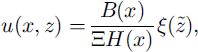
where
 and
and
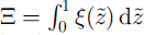
The vertical velocity field w(x, z) is found from continuity:

Differentiation of Equation (4) with respect to x yields

The chain rule and Equation (2) are used to calculate
 :
:

Substitution of Equation (7) into Equation (6) and integration with respect to z with the boundary condition of zero velocity at
 , yields the vertical velocity w:

The calculation of particle paths is simplified if calculations are performed on a regular grid in the normalized vertical coordinate
 . The vertical motion of an ice particle in this transformed domain is then described by the material time derivative
 which is related to w = dt
z by
which is related to w = dt
z by

and reduces to

Equations (4) and (10) describe a continuous flow field for ice particles given ice thickness H(x), bedrock geometry R(x), shape function
 and accumulation pattern b(x). Ice thickness and bed geometry are given by the RES measurements. R(x) is smoothed so that H(x) is smooth and slowly varying. The shape function
 is described by an eighth-order Chebyshev polynomial fit to the typical flank shape function predicted by a steady-state, two-dimensional, finite-element model (FEM) of flow at Siple Dome (Reference Nereson, Waddington, Raymond and JacobsonNereson and others, 1996). The FEM shape function was chosen because it includes a correction for typical temperature distribution in the ice. Other shape functions, such as the common description for “laminar ice flow” (e.g. Reference PatersonPaterson, 1994), could also be used.
The form of the accumulation pattern b(x) is chosen to allow the maximum number of degrees of freedom where we expect the accumulation pattern to vary the most, while maintaining calculation efficiency. Since the divide is the main topographic feature in the region, large gradients in the spatial pattern of accumulation may be expected to occur there, with relatively smooth variation elsewhere. We choose to represent the accumulation pattern by an arctangent function,

where b(0) is the accumulation rate at the divide in ice-equivalent units and d = (s, n) denotes values for the south and north sides of the divide. In the limit of small λ d, this function approaches a step function at the divide. At large λd (> 50 km), this function approaches a constant gradient over the calculation domain. Different values for λd and amplitude αd for the south (s) and north (n) sides of the divide can accommodate a wide range of accumulation patterns. We set b(0) = 0.11 m a−1 according to measurements made on a shallow ice core near the summit in 1994 (Reference Mayewski, Twickler and WhitlowMayeski and others, 1995; Reference KreutzKreutz and others, 1999). However, b(0) only serves to scale the flow field, and does not define the shape of the flow field. Since we are interested in the spatial pattern of accumulation relative to the accumulation rate at the divide, the particular choice for b(0) is not critical to the calculation of isochrone shapes.
Ice particles originating at the surface are tracked through time according to the velocity field given by Equations (4) and (10) and the accumulation pattern given by Equation (11). The resulting age field is contoured to obtain the resulting internal layer pattern. The parameters, α s, α n, λ s and λ n, are varied in order to find the combination that produces the best match to the observed layer shapes.
Misfit Calculation
For each model calculation, a set of isochrone shapes is predicted for given amplitudes (α
s, α
n) and transition lengths (λ
s, λ
n) of the spatial accumulation function (Equation (11)). Since the actual age vs depth relationship is unknown, the goal is to match the shapes of all observed internal layers, and not any particular isochrone. Therefore, we are free to decide which modeled layer to compare to a given observed layer shown in Figure 3. Following Reference Nereson, Raymond, Waddington and JacobelNereson and others (1998a), the shapes of modeled and observed layers with the same average height are compared. The shape of a given modeled (M) or observed (O) layer, denoted by the index j, is quantified by measuring its elevation at each horizontal position i relative to its average elevation
 :
:

An analogous equation defines the shape of observed layers
 . Each side of the divide is considered separately. The superscript d =(s, n) denotes values for the south (s; xi
< −3 km) and north (n; xi
> 3 km) sides of the divide, respectively. No attempt is made to match the observed layers in the divide zone xi
= ±3 km. The anomalous flow in this zone cannot be described by a simple flow field and is therefore not accounted for in the current model.
. Each side of the divide is considered separately. The superscript d =(s, n) denotes values for the south (s; xi
< −3 km) and north (n; xi
> 3 km) sides of the divide, respectively. No attempt is made to match the observed layers in the divide zone xi
= ±3 km. The anomalous flow in this zone cannot be described by a simple flow field and is therefore not accounted for in the current model.
Modeled isochrone shapes
 are compared to the observed isochrone shapes
 using a misfit parameter Jd
which is also calculated separately for each side of the divide for each model calculation:
using a misfit parameter Jd
which is also calculated separately for each side of the divide for each model calculation:

The term ϵj
is the expected combined error from the model and the data for a particular layer j. A depth-dependent weighting function ωj
for layer j is chosen to account for the fact that the layers are not uniformly distributed over depth. The number Nj
is the total number of points i along a layer j, L = 14 is the total number of layers and p = 1 is one less than the number of free parameters in the model. This parameter p allows the comparison of misfit parameters arising from models which use different numbers of free parameters. The total number of points is
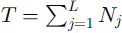 . In this application, each layer is sampled every 1000 m, and Nj
depends on the length of the RES profile (30–50 km).
. In this application, each layer is sampled every 1000 m, and Nj
depends on the length of the RES profile (30–50 km).
Separation of the problem into northern and southern portions eliminates the need to search a four-parameter space (λs , λn , αs , αn ) to minimize the residual. Our more computationally efficient approach requires searching a two-parameter space for each side of the divide. A consequence of this approach is that we do not necessarily compare northern and southern portions of the same modeled isochrone to a given observed isochrone. However, since the northern and southern portions of modeled layers are linked at the divide by the depth–age relation associated with the scale accumulation rate b(0) and ice thickness H(0), the independently determined results for the north and south side of the divide can be combined.
The error term ϵj
represents errors in layer shape arising from errors in estimating z and
 for the modeled and observed layers. We do not account for contributions to the total error from model simplifications. These errors are difficult to quantify and are addressed instead using sensitivity tests developed in a later section. Errors in the observed layer shapes arise from digitizing and defining a given layer and depend primarily on signal frequency, sampling density and the reflection strength of the layer. All the data used for this analysis were collected at the same frequency (2 MHz) and spatial density (100 m). As the reflection strength of the layer decreases, it becomes more difficult to identify from RES data. Layers identified using the automatic picking routine are rougher as the reflection strength decreases. An error is therefore associated with picking a layer and is assumed to be proportional to the “roughness” of the layer, defined as the standard deviation of the difference between the smoothed and raw internal layer shape. This standard deviation for Siple Dome data varies between 1 and 5 m, increasing with layer depth. We estimate the combined error ϵj
at 6–10 m, depending on layer depth.
for the modeled and observed layers. We do not account for contributions to the total error from model simplifications. These errors are difficult to quantify and are addressed instead using sensitivity tests developed in a later section. Errors in the observed layer shapes arise from digitizing and defining a given layer and depend primarily on signal frequency, sampling density and the reflection strength of the layer. All the data used for this analysis were collected at the same frequency (2 MHz) and spatial density (100 m). As the reflection strength of the layer decreases, it becomes more difficult to identify from RES data. Layers identified using the automatic picking routine are rougher as the reflection strength decreases. An error is therefore associated with picking a layer and is assumed to be proportional to the “roughness” of the layer, defined as the standard deviation of the difference between the smoothed and raw internal layer shape. This standard deviation for Siple Dome data varies between 1 and 5 m, increasing with layer depth. We estimate the combined error ϵj
at 6–10 m, depending on layer depth.
The weight function ωj is applied to correct for the fact that the measured internal layers are unevenly spaced with depth. With no imposed weighting, areas where layers are closely spaced would be weighted more heavily than areas where layers are sparse. We define ωj to be proportional to the distance between a given layer j and its adjacent layers with a scale factor F so that

More weight is given where the vertical space between adjacent layers is greater. The scale factor F is chosen so that

With this weighting scheme, each unit of cross-sectional area receives equal weight. Since depth and age are not linearly related, this does not give equal weight to all time represented by the internal layers. Younger ages are weighted more heavily according to the depth–age relationship. Since the weight function ωj is scaled by F, modeled layers which match the observed layers to within the weighted error will produce Jd < 1.
Results
Predicted steady-state accumulation pattern
Figure 4 shows the range of steady-state accumulation patterns which fit the observed layers to within given error intervals. The black range corresponds to values of λs , λn , αs and αn which produce a match to within the estimated errors in the data (Jd < 1). The medium and light ranges correspond to Jd < 2 and Jd < 3, respectively. The best match between the model and the data is produced with a south–north accumulation gradient given by the parameters λs = 50 km, λn = 5 km, αs = 0.8 and αn = 0.2. Relative to the divide, the minimization predicts 40% lower accumulation rates at 30 km south of the divide and 15–40% higher accumulation rates at 30 km north of the divide. The minimization predicts a narrow range of possible accumulation patterns south of the divide and a broad range north of the divide (Fig. 4). The broad range north of the divide arises because the layers (and hence the best-fitting accumulation pattern) are relatively flat outside of the divide zone (x > 3 km). Since we exclude the divide zone in our analysis, any accumulation pattern with little or no gradient outside the divide zone produces a good match to the observed layers. This allows the possibility of very high accumulation gradients in the divide zone. Previous analyses of layer shapes in the Siple Dome divide zone show evidence for large accumulation gradients (5–7 × 10⁻⁶ a−1) within 2–4 km of the divide (Reference Nereson, Raymond, Waddington and JacobelNereson and others, 1998a).
Steady-state accumulation pattern which produces the best fit to the observed layer shapes. The black range produces layers which match the data to within the expected errors (Jd< 1). The dark- and light-gray ranges corresponds to Jd < 2 and Jd < 3, respectively. The accumulation pattern is scaled to the accumulation rate at the divide (b(0) =0. 11 m a−1 in ice-equivalent units).

Figure 5 shows the predicted layer shapes given a spatially constant accumulation pattern (panel a) and given the best-fit accumulation pattern (panel b). The improved match to the observed layer shapes from using the best-fit spatial pattern is apparent. The remaining mismatch at x = 30–40 km is probably due either to over-smoothing of the bed topography to ensure that the ice thickness is slowly varying in x, or to three-dimensional flow effects which are not taken into account by the model.
(a) RES-detected layer shapes (gray) compared to layer shapes calculated assuming a constant accumulation pattern (black). For the purposes of display, modeled layers shown match the measured layers near the divide. In the residual calculation, modeled and measured layers with the same average depth are compared. (b) RES-detected layer shapes (gray) and layer shapes calculated assuming the steady-state accumulation pattern which produces the minimum weighted mismatch Jd (black). For each side of the divide, modeled and measured layers have the same average depth. The modeled layers shown correspond to the parameters λs = 50 km, λn = 5 km, αs = 0.8 and αn = 0.2. Modeled layer shapes within 3 km of the divide are ignored because the anomalous flow regime associated with ice divides is not accounted for in the ice-flow model.

Comparison with other measurements
The inferred accumulation gradient is consistent with accumulation estimates from chemical analysis of 2 m snow pits at ± 30 km (Reference Kreutz, Mayewski, Twickler, Whitlow and MeekerKreutz and others, 1997), but inconsistent with measurements of burial rates of survey poles over a 1 or 2 year period (Fig. 6) and with the accumulation pattern deduced from the physical and electrical stratigraphy of three 100 m cores taken from ±30 km and at the divide (personal communication from K. Taylor, 1998). Preliminary analysis of the shallow cores suggests a smaller gradient with 15–25% less accumulation at 30 km south of the divide than at 30 km north of the divide. However, these methods sample different time-averaged windows at Siple Dome. Burial rates of survey poles measure accumulation over 1 or 2 year periods; snow pits span < 10 years; shallow cores at Siple Dome span time-scales of 10 to nearly 1000 years; the RES layers in Figure 3 are detected approximately every 1000 years in the shallow ice and every 10 000 years in deep ice. The shallowest RES layer does not overlap with shallow core measurements. Our estimate of the spatial accumulation pattern represents the pattern averaged over at least 1000 years, and may not agree with the pattern averaged over decades or centuries. It is therefore questionable to validate our estimate with measurements from shallow cores and snow pits.
The accumulation pattern inferred from the RES layer shapes is denoted by the shaded area. Dark and light areas correspond to Jd < 1, Jd < 2, and Jd < 3, respectively. The flux divergence calculated from GPS measurements of horizontal velocity is shown by the lined region. Diamonds denote accumulation-rate estimates in ice-equivalent units from survey-pole burial rate measurements in 1994, 1996 and 1997.

If Siple Dome is steady-state as we assume, then the spatial accumulation pattern b(x) should match the spatial pattern of the horizontal flux divergence
 determined from GPS measurements of survey pole velocity (Reference NeresonNereson, 1998) and RES measurements of ice thickness:

This comparison can be used to determine whether the inferred accumulation pattern is consistent with the assumption of steady-state flow and geometry. Figure 6 shows that the inferred accumulation pattern and the calculated flux divergence pattern generally agree north of the divide between 0 and 20 km before the flow begins to turn off the pole line. The patterns strongly disagree south of the divide. This disagreement suggests that Siple Dome is presently not in steady state and may be significantly thickening along its south flank. Reference NeresonNereson (2000) suggests that this non-steady situation along the flank is probably recent, existing for < 500 years, and is consistent with the finding that the summit area is presently near steady state (Reference NeresonNereson, 1998; Reference Raymond, Nereson, Scambos, Jacobel and ConwayRaymond and others, 1998). Since the shallowest internal layer used to infer the accumulation-rate pattern is about 1000 years old, the pattern of accumulation inferred from this analysis reflects the long-term pattern and is not significantly affected by the recent non-steady situation.
Temporal changes in spatial accumulation pattern
A steady-state spatial accumulation pattern matches the observed layers to within the expected errors. However, it is possible that the spatial pattern has changed with time and that the effects of these changes on the internal layer pattern are indistinguishable from the steady-state case. Could a non-steady-state spatial pattern of accumulation also match the observations?
If a detectable change in the accumulation pattern has occurred, then an accumulation pattern which produces a good match to shallow (young) layers would not produce a good match to deep (old) layers. We examine the depth distribution of the misfit to test this possibility. The misfit values along each layer are averaged and the amplitude values αs and αn are varied while the transition length values λs and λn are held fixed at 50 and 5 km, respectively. By examining the effects of varying the amplitude variable α, we are looking for temporal changes in the spatial accumulation gradient across the dome and assuming the general shape (e.g. transition length λ) of the pattern does not change significantly over time. The matrix of horizontally averaged misfit parameters vs average layer height and vs amplitude value is interpolated at a finer resolution for display purposes. The result is shown in Figure 7 for north and south sides of the divide.
Depth distribution of residuals for layers south and north of the divide. South of the divide, minimum residuals are found at one amplitude value αs at all depths, suggesting no change over time. North of the divide, residuals for shallow (young) layers are minimized at low values for αn while residuals for deep (old) layers are minimized at slightly larger values. Transition values λs and λn are fixed at 50 and 5 km, respectively.

In Figure 7 the panel corresponding to the south side of the divide shows that layers at all depths have minimum residuals for a single amplitude value. This suggests that there has been no change in the amplitude value (and therefore accumulation pattern) over the time represented by the measurements. The panel corresponding to the north side of the divide shows a very broad minimum around an amplitude value of 0.2, suggesting little or no change in the accumulation pattern over time. However, there appears to be a trend to the minimum, with shallow layers fitting best to a lower value of αn and deeper layers fitting best to a slightly higher value of αn . This change with depth shows that the data allow for the possibility that the accumulation gradient north of the divide has decreased over time. Figure 8 shows the range of time-dependent accumulation patterns implied by the misfit pattern shown in Figure 7 assuming model-predicted time-scales for Siple Dome to date the internal layers (Reference Nereson, Waddington, Raymond and JacobsonNereson and others, 1996). This accumulation scenario suggests that prior to 5–7 kyr BP, accumulation rates on the northern flank were 15–30% higher relative to the divide than in more recent times. The accumulation gradient north of the divide has possibly decreased over the past 10 kyr. However, we cannot distinguish between the time-dependent (Fig. 8) and steady-state (Fig. 4) scenarios, since the range of time-dependent accumulation patterns shown in Figure 8 is within the range of inferred steady-state patterns that produce Jd < 1. Because data for deep layer shapes north of the divide are sparse, the time-dependent scenario shown in Figure 8 should be viewed with caution. North of the divide, layers are not detectable over the full region (Fig. 3). The residuals at depth are therefore dominated by one deep layer which extends to 28 km from the divide.
Possible time change in the spatial accumulation pattern allowed by the data. Shallow layers correspond to layers younger than about 5–7 kyr. Deep layers are older than 5–7 kyr.

Nevertheless, this result is relevant to explaining the apparent migration of the Siple Dome ice divide toward Ice Stream D at 0.05–0.50 m a−1 for > 2000 years that has been inferred previously from analysis of the radar-detected layer shapes in the divide zone (Reference Nereson, Raymond, Waddington and JacobelNereson and others, 1998a). One hypothesis is that a temporal change in the spatial accumulation pattern across the dome could cause the divide migration. Analysis by Reference Nereson, Hindmarsh and RaymondNereson and others (1998b) shows that an increase in the south–north gradient is required to move the divide toward Ice Stream D. The allowed change in the spatial pattern shown in Figure 8 is a decrease in the south–north accumulation gradient over time; this change is in the opposite sense. We therefore suspect that temporal changes in the accumulation pattern are not responsible for Siple Dome divide motion. Rather, the divide motion is likely caused by changing conditions at the boundaries of Siple Dome at the margin of Ice Stream C and/or D.
To make this a firm conclusion, the ability of RES-detected internal layer shapes to record changes in the accumulation pattern over time needs to be quantified. What kinds of accumulation-pattern changes would produce a detectable change in the internal layer pattern? Is this signal distinguishable from other factors which might affect the layer shapes such as changes in ice thickness? Assuming no basal melting or significant changes in surface topography, the shape of an internal layer depends on (1) the amount and distribution of deposited snow since the layer was formed at the ice surface, and (2) the amount and distribution of strain the layer has experienced since its formation. The first depends on the accumulation pattern since the time of layer deposition, and the second depends on both the accumulation history and the thickness history of the ice sheet.
Sensitivity to Temporal Changes in Accumulation Distribution
Recovery of information about temporal changes in the spatial pattern of accumulation is limited by how well and how many internal layers are measured and how well the strain history is known. Measurements from our low-frequency RES system can detect internal horizons every 50–100 m in an ice column, corresponding to one layer every 0.5–20 kyr (for Siple Dome) with a measurement uncertainty of about 10 m (one-tenth of the dominant wavelength (82 m) of the transmitted 2 MHz signal). To be detectable, changes in the accumulation distribution must produce a change in spacing between adjacent internal layers that is greater than the measurement uncertainty. Lack of knowledge of the strain history is also a limitation. This is especially difficult to estimate for older (deeper) layers. The total strain depends on the history of the velocity field, which in turn depends on history of accumulation — the quantity we are trying to find.
A simple analytic argument can be used to quantify these factors and make an order-of-magnitude estimate of the limits of using RES-detected internal layers to estimate changes in accumulation patterns. Gonsider a perfectly plastic ice sheet. Any change in the accumulation pattern will be accommodated by a change in the velocity field with no change in the ice thickness. Suppose we sample the internal stratigraphy at two places on the ice sheet, sites I and II, separated by some distance x. Sites I and II are sufficiently close together that the ice thickness H is essentially equal at both sites. Under a uniform accumulation pattern, isochrones will appear at the same height above the bed at both sites. If a non-uniform spatial pattern exists, a given isochrone will be found at different heights. If we make the additional assumption that the ice moves only vertically, then we can predict the difference in height Δz to a particular isochrone between the two sites. A change in the spatial pattern over time will produce a deviation from the predicted steady-state height difference. Figure 9 shows this situation schematically.
Schematic of the analysis used to determine the sensitivity of internal layer shapes to a change in the distribution of accumulation.

In a real ice sheet, the total ice thickness would increase or decrease in response to a change in the accumulation rate, reducing the effect of accumulation changes on the space between internal layers. Our perfectly plastic assumption produces exaggerated Δz values. However, because of the non-linear nature of ice flow, ice thickness is relatively insensitive to accumulation changes (Reference PatersonPaterson, 1994, p. 244), so a perfectly plastic extreme is a reasonable starting point to place an upper bound on the minimum accumulation changes that can be detected in internal layers.
In addition, ice layers deposited upstream and between sites I and II would, in reality, travel horizontally as well as vertically over time, to be found eventually beneath, say, site II. Therefore, the layer-thickness pattern beneath sites I and II reflects some average of the deposition upstream of the sites, not the deposition at each site, as we assume. The following analysis applies to areas of an ice sheet where vertical ice motion is dominant, such as near an ice divide and some distance above the bed.
Suppose both sites have the same ice thickness H, and constant and uniform vertical strain rate so that

where R(x) = 0 and z then denotes distance above the bed. Let t denote the age of the ice or, equivalently, time before present, so that t = 0 is at the present ice surface. We assume site I has a constant accumulation rate b I(t) = b 0 and site II has a variable accumulation rate b II(t). Solving Equation (17) for z(t) assuming b(t) = b 0 gives the Nye depth–age relation for site I:

Site II has a time-dependent accumulation rate b II(t). Its depth–age relation is

Assume b II(t) includes a “box-car”-shaped pulse in time with center t 0, duration 2T and magnitude Δb relative to b 0 (Fig. 9). We are interested in the height of a particular isochrone at each site, and the size of the height difference between the sites (Δz(t) = z I (t) – z II(t)) for a given accumulation history at site II. We can use RES data to detect changes in the accumulation pattern between sites I and II, if the changes cause isochrones at site II to be deeper or shallower than at site I by an amount that is more than the measurement error (≈10 m for 2 MHz).
The difference in height Δz to a given isochrone between the two sites can be calculated from Equations (18) and (19) for times before, during and after the accumulation pulse at site II:

Equation (20) has four time-scales: (1) the fundamental ice-flow or vertical-strain time-scale τ = H/b 0; (2) the duration 2T of the accumulation pulse at site II; (3) age t 0 of the pulse; and (4) the time-scale H/Δb to develop a height difference Δz/H ∼ 1 in the absence of strain.
The relationship among these time-scales illustrates that there are competing processes involved in creating a Δz/H signal. In the absence of layer thinning from ice deformation, a Δz/H signal for any layer with age t * grows in proportion to the total amount of additional accumulation deposited at site II since t = t *. The maximum amount is proportional to 2T(Δb/H). However, vertical strain causes all layers to thin exponentially with age in proportion to exp(−t/τ); since the layers must conform to the bed, the Δz/H signal also decays exponentially. Thus, the maximum Δz/H value is reached at an intermediate depth, marking a transition between growth and decay of the Δz/H signal.
In the limiting case where duration 2T of the box-car pulse is infinitely long (i.e. b II(t) = b 0 + Δb), Δz/H can be calculated directly from Equations (18) and (19) (see Fig. 10):

The critical age τ c at the growth/decay transition depth can be calculated by differentiating Equation (21) with respect to t and solving for t = τ c when ∂t Δz = 0:

For Δb ≪ b 0, a Taylor series expansion of ln(1 + Δb/b 0) shows that rc is approximately equal to the fundamental time-scale τ = H/b 0. Substituting t = τ c ≈τ into Equation (21) gives the limiting value for Δz/H,

For a given accumulation pulse amplitude Δb, it is impossible to create a Δz/H signal greater than this limiting value. Figure 10a illustrates this by showing Δz/H signals, calculated from Equation (20), arising from three box-car pulses of accumulation of a given size Δb, each with a different duration 2T, assuming t 0 = T. More generally, any box-car pulse of accumulation with a duration 2T greater than the transition time τ c is associated with a limiting value for Δz/H according to

In the limit as t 0 → T, Expression (24) reduces to Expression (23).
Top row shows four groups of accumulation histories at site II, relative to site I. Middle row shows the difference in height Δz/H to a given isochrone vs scaled isochrone age. Bottom row shows Δz/H vs height above the bed z/H. For the RES data from Siple Dome, the detection limit is Δz = 0.01 H (about 10 m).

When the duration 2T is less than the growth/decay transition time τ c, growth of Δz/H is limited by the characteristics and age of the accumulation pulse. The layer height difference Δz/H reaches a maximum value in the layer dating to t = t 0 + T, when the pulse started. For short pulses (2T ≪ H/Δb), Equation (20) gives

The maximum Δz/H value is proportional to the product of 2T and Δb/H, which is the area under the curve bII(t)–b 0. The same maximum Δz/H value can be obtained with a relatively large accumulation pulse of short duration or a small pulse of long duration. The signal decays exponentially according to the relative age t 0/τ of the pulse. Figure 10b shows the Δz/H responses to two identical accumulation pulses at site II occurring at different times t 0. Recent changes produce a larger Δz/H signal at depth. The scenario denoted by the dashed curve in Figure 10a would not be detected with a measurement error in Δz as large as 1% of the ice thickness (e.g. 10 m for Siple Dome where H = 1000 m).
If 2T = H/Δb, then at the limit as 2T → 0, Equation (20) describes the unit impulse response of the layers to an accumulation change (Reference NyeNye, 1965). The impulse-response function can be used to find Δz/H for any combination of accumulation pulses at site II. Figure 10c shows how different changes in the spatial accumulation pattern can produce a similar signal in the internal layer pattern. Long, low-amplitude changes such as a small pulse of long duration (thick dashed curve) could produce a similar signal to several high-amplitude, frequent pulses (solid curve). Since the areas under the b II(t) curves are similar, we expect the Δz/H values to be similar. For comparison, the height difference arising from an accumulation pattern where site II has higher accumulation rates for all time (2T → ∞) is shown (thin dashed curve). This scenario gives a similar maximum value for Δz/H, but the variation of Δz/H with depth is distinctly different.
Figure 10d shows the response of the layers to a gradual increase in the accumulation rate at site II (dotted curves). According to the scale values appropriate for Siple Dome (b 0 = 0.10 m a−1 and H = 1000 m), the thick and thin dashed curves correspond to different ages of the onset (2000 and 5000 years BP). Both increase at a prescribed rate (1 × 10⁻⁵ m a−2) which is toward the low end of the range required to move the Siple Dome divide (0.2–3.0 × 10⁻⁵m a−2; Reference Nereson, Hindmarsh and RaymondNereson and others, 1998b), assuming that sites I and II are 20 km apart. The figure shows that if the spatial accumulation-rate gradient has been steadily increasing at this rate for the past 2000–5000 years, a detectable signal (Δz > 10 m) should be observed in the internal layer pattern. If such an increase in the spatial accumulation gradient occurred more recently than 1500 years ago, the signal would be below our detection limit. Also plotted in Figure 10d is the predicted response to a step-change occurring 3000 years before present (solid curve). The predicted response of the layers to this step-change is not distinguishable from a gradual change that began 5000 years ago.
Some general conclusions can now be drawn from this order-of-magnitude sensitivity exercise.
-
1. Recovery of information about past accumulation patterns from RES-detected internal layer shapes is limited by the sparseness of data, the measurement error and the way this information is recorded in the internal layer pattern.
-
2. If δ is the measurement error for Δz, changes in the accumulation pattern where Δb/b 0 < eδ/H are never detectable (Equation (23)).
-
3. If the duration 2T of the accumulation pulse is long (> τ c), then the maximum Δz signal reaches a limiting value given by Equation (23). When 2T < τ c, the maximum Δz/H signal depends on the product of the size Δb and duration 2T of the pulse (Equation (25)). A small change in the spatial pattern of accumulation of long duration (∼ τ c) can produce the same maximum Δz/H value as a large change of short duration (≪τ c). It may be possible to distinguish between these scenarios from the depth variation of Δz/H.
-
4. The problem is non-unique: it is possible for different accumulation histories to produce indistinguishable cumulative-strain and internal layer patterns. Even if an infinite number of internal layers could be measured, the recovery of past changes would still be limited because the cumulative strain of a given layer depends on the accumulation history since its deposition. As a result, it is difficult to distinguish between a gradual change in the accumulation pattern and a step-like change, even for the shallowest layers.
-
5. It is likely that the change in the spatial pattern of accumulation required to cause Siple Dome divide migration (Reference Nereson, Raymond, Waddington and JacobelNereson and others, 1998a) would be detectable in the Siple Dome RES layer shapes if it occurred.
Sensitivity to Changes in Ice Thickness
All analysis to this point has assumed constant ice thickness over time. However, Siple Dome is located in a dynamic area of the West Antarctic ice sheet, and it is likely that its thickness and configuration were different in the past. One hypothesis is that the whole Siple Coast was much thicker during the Last Glacial Maximum (≈ 20 kyr BP) and has subsequently thinned via retreat of the grounding line and/or initiation of ice-stream activity. Initiation of ice-stream flow at the edges of what is now Siple Dome could cause a wave of rapid thinning to propagate inward from the ice-stream margins to the present divide, analogous to the predicted thinning wave associated with a potential drop in sea-level for East Antarctica described by Reference Alley and WhillansAlley and Whillans (1984). The effect of such thinning on the internal layer pattern and associated implications for the inferred accumulation pattern are not immediately clear.
We use a coupled surface-evolution and particle-tracking model (e.g. Reference WaddingtonWaddington, 1982) to determine the effect of rapid thinning of Siple Dome on the internal layer pattern. The surface-evolution model uses a finite-difference scheme to solve the continuity equation:

In this application, we consider a flat-bed ice sheet (R(x) = 0) deforming as an isothermal, parallel-sided slab so that the variation of horizontal velocity u with height above the bed z is

where
 in Equation (2) reduces to
 , the flow parameter A = 0.5 × 10⁻¹⁷ Pa3 a−1, Glen’s flow-law exponent n = 3, ice density ρ = 917 kg m−3, and gravity g = 9.8 m s−2. Ice flux q can be written in terms of the ice-thickness profile H as:

Equation (26) is solved with an explicit numerical scheme on a finite-difference grid with spacing of 2 km (about twice the ice thickness), a time-step of 1 year and a prescribed accumulation history b(x, t). The initial profile is a symmetric two-dimensional ice divide, 1500 m thick at its center, corresponding to a Vialov profile (Reference VialovVialov, 1958) with spatially constant accumulation rate b(x) = 0.10 m a−1, and truncated at 50 km from the divide. The flux is calculated at the midpoint of each gridcell as recommended by Reference WaddingtonWaddington (1982). The ice thickness is prescribed at the boundaries of the domain. Ice thickness at the lateral boundaries is rapidly increased or decreased at a prescribed rate to simulate changes in ice-stream activity.
A separate particle-tracking model takes as input the geometry H(x, t) and depth-averaged horizontal velocity field
 from the surface-evolution model at 100 year intervals and interpolated to a 20 year time-step using Chebyshev polynomials. The vertical velocity field is determined from incompressibility,

The total velocity field is thus given by


where
 . Ice particles originating at the surface are tracked in this time-dependent velocity field for 10–15 kyr using a time-step of 20 years. The age field is then contoured to reveal the shape of the internal layer pattern.
Figure 11 shows the internal layer shapes 3000 years after the initiation of a rapid synchronous thinning of the ice streams on either side of the divide at a rate 5b (0.5 m a−1) for 1000 years. This thinning affects the shapes of internal layers such that the thinning scenario predicts generally flatter internal layers than the steady-state case. The relative flatness occurs because prior to thinning, the ice sheet itself was flatter and the internal layers at depth contain some “memory” of this former geometry. Isochrone shapes from the thinning scenario which match those from the steady-state scenario at the divide are up to 15 m shallower 40 km from the divide. If such thinning occurred at Siple Dome, our inferred accumulation rate on the flanks of the dome would be too low. Since rapid synchronous thinning driven at the edges of the dome has only a modest effect on the layer shapes, the effect of gradual thinning would be minimal. The main effect of the thinning is to alter the age and annual-layer thickness distribution (Fig. 11c). Measurements of the depth–age relationship, annual-layer thicknesses and 10Be (a proxy for accumulation rate) (e.g Reference SteigSteig, 1997; Reference Steig, Morse, Waddington and PolissarSteig and others, 1998) from the deep ice core would help determine whether thinning has occurred.
The effect of a symmetric change in ice-sheet thickness on internal layer shapes for a 500 m thinning which begins 3000 years BP. (a) Surface profiles at 100 year intervals. Thinning at the boundaries is complete after 1000 years, with full adjustment of the surface after 4000 years, (b) Internal-layer shapes from the steady-state (solid) and thinning (dashed) scenarios. Displayed layers from each scenario are chosen so that their height matches at x = 0. They do not represent the same age. (c) Age vs depth relationship at x = 0 for the steady-state case (solid) and the thinning scenario (dashed).

Figure 12 shows that rapid asynchronous or asymmetric thinning at the boundaries of the dome would significantly affect the internal layer pattern. Layers on the thinning side of the divide would appear shallower than in the steady-state case, and we would under-predict accumulation rates there. Layers observed on the south flank of Siple Dome appear to exhibit this feature since they are significantly shallower than layers on the north flank. Is this feature a signal of asynchronous thinning rather than the spatial variation of accumulation? One consequence of such asymmetric thinning would be rapid movement of the ice divide. However, the presence of a convex-up bump feature in the near-divide layer pattern (Reference Nereson, Raymond, Waddington and JacobelNereson and others, 1998a) suggests that the divide has been within a few ice thicknesses of its present position for at least the past few thousand years. Therefore, major asynchronous thinning of Siple Dome in the past several thousand years is not likely. We conclude that the spatial accumulation pattern and not asynchronous thinning is the cause of the shape of the shallow layers south of the divide.
The effect of an asymmetric change in ice-sheet thickness on internal layer shapes for thinning which begins 3000 years BP. (a) Surface profiles at 100 year intervals. Thinning at the boundaries is complete after 1000 years, with full adjustment of the surface after 4000 years. (b) Internal-layer shapes from the steady-state (solid) and thinning (dashed) scenarios. Displayed layers from each scenario are chosen so that their height matches at x = 0. They do not represent the same age. (c) Age vs depth relationship at x = 0 for the steady-state case (solid) and the thinning scenario (dashed).

Conclusions
We use a steady-state ice-flow model and minimization scheme to estimate the pattern of accumulation over Siple Dome from the observed pattern of internal layering. Relative to the divide, the model predicts 40% less accumulation 30 km from the divide on the south flank of Siple Dome, and about 15–40% more accumulation 30 km from the divide on the north flank. The pattern is consistent with the hypothesis that storms approaching Siple Dome from the north deposit most of their moisture on the windward side of the dome as a result of orographically induced uplift (e.g. Reference BromwichBromwich, 1988). Because the predicted pattern produces a match to the observed internal layer shapes at all depths to within errors, it is possible that the accumulation pattern has not changed in the past 10 kyr. However, the data do allow for a relative 15–30% decrease in the accumulation rate north of the divide sometime during the period 5–15 kyr BP.
Certain changes in the accumulation pattern over the past 10 000 years should produce a detectable signal in the internal layer pattern. Because RES layers sample the time domain infrequently (every 1000–10 000 years) and because the internal layer shapes lose memory of changes in the spatial pattern of accumulation, long, low-amplitude changes can be indistinguishable from a series of short, high-amplitude changes. Our sensitivity calculations show that relatively small changes in the spatial pattern (Δb ≪ b 0) that are of long duration (2T > τ) will displace internal layers by an amount proportional to Δb/b 0 according to Expression (24). Ghanges of shorter duration will displace internal layers in proportion to the size and duration of the change (Expression (25)).
Synchronous thinning at the edges of the ice sheet would leave a minimal signal in the layer shapes, making them shallower toward the dome margins than predicted under steady state. If such thinning has occurred, our analysis would under-predict the relative accumulation rate far from the divide. Significant asynchronous thinning (e.g. at a rate ∼5b 0) would significantly affect layer shapes. However, even small asymmetric changes would be accompanied by significant shifts in the divide position (Reference HindmarshHindmarsh, 1996; Reference Nereson, Hindmarsh and RaymondNereson and others, 1998b). Since there appear to have been no dramatic shifts in the divide position over the past several thousand years (Reference Nereson, Raymond, Waddington and JacobelNereson and others, 1998a) and since the dome does not appear presently to be dramatically thinning or thickening (Reference NeresonNereson, 1998; Reference Raymond, Nereson, Scambos, Jacobel and ConwayRaymond and others, 1998) we do not believe that asynchronous thinning at the boundaries of Siple Dome has significantly affected the layer shapes for at least the past several thousand years. However, we cannot rule out this possibility for older times without independent evidence.
Our results are relevant to the possible cause of northward migration of the Siple Dome ice divide inferred previously from analysis of radar layer shapes in the divide zone (Reference Nereson, Raymond, Waddington and JacobelNereson and others, 1998a). If a gradual increase in the south–north accumulation gradient at 0.1–1.5 × 10⁻⁹a−2 is the cause of the divide migration (Reference Nereson, Hindmarsh and RaymondNereson and others, 1998b), this signal should be detectable in the internal layer pattern. The internal layers at Siple Dome show no evidence for an increase in the accumulation gradient of this magnitude over the past 2–5 kyr. Such a change would appear in the pattern of residuals shown in Figure 7. The spatial pattern of residuals allows only for a decrease in the accumulation gradient sometime during the past 5–15 kyr. Although changes in the accumulation gradient at the low end of the range 0.1–1.5 × 10⁻⁹ a−2 since 1500 years BP are not detectable in our data, the existing evidence argues against changes in the accumulation pattern as the main cause of Siple Dome divide migration.
Acknowledgements
This work was funded by U.S. National Science Foundation grants OPP-9316807, OPP-9316338 and OPP-9420648. We are grateful to H. Conway, A. Gades and T. Scambos for their valuable contributions to the fieldwork at Siple Dome, and to C. S. Hvidberg and F. Ng for their thoughtful comments as reviewers, which led to significant improvements in the manuscript.



