2.1. Frontal position data

Outlet glacier frontal positions were obtained primarily from synthetic aperture radar (SAR) image mode precision data. Imagery was supplied by the European Space Agency (ESA), acquired as part of the European Remote-sensing Satellite-1 (ERS-1), ERS-2 and Envisat missions. Following Carr and others (2013b), data were processed by applying precise orbital state vectors, and radiometric calibration was applied. Images were then multi-looked to reduce speckle and terrain-corrected using version 2 of the 30 m resolution Advanced Spaceborne Thermal Emission and Reflection Radiometer (ASTER) global digital elevation model (GDEM). Owing to the higher geolocation accuracy of the Envisat data, ERS images were co-registered with corresponding Envisat scenes. SAR imagery was supplemented with visible Landsat imagery where possible, which was provided by the United States Geological Survey (USGS) Global Visualization Viewer (http://glovis.usgs.gov/). For both imagery types, scenes were selected as close as possible to the end of the calendar month, to allow for comparison with monthly means of atmospheric and oceanic data. Landsat imagery was provided at a spatial resolution of 30 m and the SAR imagery was output with a cell size of 37.5 m.

Frontal position variations were measured using a previously employed method, whereby the glacier terminus was repeatedly digitized within a fixed reference box (e.g. Reference Moon and JoughinMoon and Joughin, 2008; Reference Howat, Box, Ahn, Herrington and McFaddenHowat and others, 2010; Reference McFadden, Howat, Joughin, Smith and AhnMcFadden and others, 2011; Reference Carr, Vieli and StokesCarr and others, 2013b). The box was aligned approximately parallel to the ice-flow direction at the glacier terminus and extended from an arbitrary upstream reference line. The terminus was then digitized from successive images and the change in area was divided by the width to calculate the change in frontal position. Retreat rates were calculated relative to the frontal position between 24 June and 8 July 1992, with the exact date depending on data availability. Glaciers for which frontal positions were available for multiple images during this time period showed no discernible change. We first calculated total retreat rates for the study period (19922010). We then divided the period into three approximately equal portions, within the constraints of data availability, in order to investigate changes in retreat rates over time. Retreat rates were therefore calculated for the time periods 1992–2000, 2000–05 and 2005–10. Frontal position data were obtained at a monthly to annual resolution, as image availability varied between glaciers.

Fig. 2.

Outlet glacier retreat rates on the northern ice cap, Novaya Zemlya, for the periods (a) 1992–2010, (b) 1992–2000, (c) 2000–05 and (d) 2005–10. Retreat rates are symbolized according to terminus type: land-terminating (triangles) and marine-terminating (circles). The magnitude of frontal position change is symbolized according to colour (purple through to yellow = retreat; greens = advance) and symbol size (larger symbols = higher retreat rate). Note that the colour and size scales are nonlinear. Outlet glacier catchments are shown in dark grey: data were provided by G. Moholdt (2012) and are part of the Randolph Glacier Inventory (Reference Gardner, Moholdt, Arendt and WoutersArendt and others, 2012). Glacier abbreviations are derived from the World Glacier Inventory, where available, and split termini are numbered sequentially (1 = main terminus, 2 = secondary terminus). Unnamed land-terminating glaciers were given the prefix ‘NZL’ and numbered sequentially. Abbreviations of glacier names are as follows (from south to north): Barents Sea coast: VIJ: Vil’kitskogo Juz; VIS: Vil’kitskogo Sev.; KRI: Krivosheina; ARK: Arkhangelskolgu; KRA2: Kraynij2; KRA1: Kraynij 1; TAI1: Taisija 1; TAI2: Taisija 2; CHE: Chernysheva; SH: Shokalskogo; CHA: Chaveva; RYK: Rykachova; VEL: Vel’Kena; MAK: Maka; VOE: Voejkova; BRO: Brounova; ANU: Anuchina; VIZ: Vize; and INO: Inostrantseva. Kara Sea coast: VYL1: Vylki 1; VYL2: Vylki 2; SHU2: Shury 2; SHU1: Shury 1; NII; Niiga; KRO: Kropotkina; MG: Moshnyj; NAL: Nalli; VER: Vershinskogo; ROZH: Rozhdestvenskogo; SRE: Srednij; and ROZE: Roze. (a) Location of study area and meteorological stations.

The mean error in marine-terminating outlet glacier frontal position was evaluated by repeatedly digitizing 16 sections of rock coastline from a subsample of five ERS, five Envisat and five Landsat images, where there should be no discernible change in coastline position between scenes (Reference Carr, Vieli and StokesCarr and others, 2013b). The resultant total mean error in frontal position was 25.3 m for marine outlets, which can be primarily attributed to manual digitizing errors and accounts for errors in image geolocation and co-registration. Frontal positions for land-terminating outlets are subject to an additional error source, which results from the comparative difficulty in identifying land-based termini from radar imagery, as the land-ice boundary is less distinct than the ocean-ice interface. Consequently, we assessed this additional error source by repeatedly digitizing the same termini from the same image, for a subsample of five ERS and five Envisat images. The resultant additional error was 67.8 m and the total error for land-terminating outlets was 72.4 m.

2.2. Atmospheric and oceanic data

Atmospheric and oceanic data were obtained from a variety of sources and used to calculate seasonal and annual mean values for individual glaciers and for each coast. Surface air temperature data were obtained from Malye Karmakuly (72°20’50” N, 52°43’34” E) and Im. E.K. Fedorova (70°27’8” N, 59°3’13’’ E) meteorological stations (Fig. 1). Data were provided at a monthly temporal resolution by the Hydrometeorological Information, World Data Center Baseline Climatological Data Sets (http://meteo.ru/english/climate/cl_data.php). Meteorological station data are sparse on NVZ, and Malye Karmakuly and Im. E.K. Fedorova are the only stations with sufficient data to assess interannual air temperature trends during the study period. However, these stations are located ~400 and ~525 km, respectively, from the study glaciers, and therefore we also used monthly air temperature data products from the US National Centers for Environmental Prediction/US National Center for Atmospheric Research (NCEP/NCAR) reanalysis 1 (Reference KalnayKalnay and others, 1996) and the European Centre for Medium-Range Weather Forecasts (ECMWF) Interim Re-analysis (ERA-Interim) data (Reference DeeDee and others, 2011).

NCEP/NCAR reanalysis data have a spatial resolution of 2.5° (about 230 km x 280 km at 76° N) and were provided by the National Oceanic and Atmospheric Administration (NOAA)/Office of Oceanic and Atmospheric Research (OAR)/Earth and Space Research Laboratory (ESRL) Physical Sciences Division (PSD), Boulder, CO, USA (http://www.esrl.noaa.gov/psd/data/gridded/data.ncep.reanalysis.html). ERA-Interim data were produced by the ECMWF and have a spatial resolution of 0.75° (about 70 km x 80 km at 76° N). In both cases, we used air temperature data from the 700 hPa geopotential height, as opposed to 2 m height, as these values correlate better with ground station data elsewhere in the Arctic (personal communication from A. Gardener, 2013) and limit the influence of SSTs on surface temperatures (Reference Gardner, Moholdt, Arendt and WoutersMoholdt and others, 2012). Air temperature values were extracted from all grid squares containing the study glaciers, and mean annual and mean summer (June-August) values were calculated. The pattern of air temperature variation was very similar between the two data products, which were strongly correlated (r =0.90, p <0.01), and differences in absolute values most likely result from their differing spatial resolution. Owing to the location of meteorological stations and the spatial resolution of the reanalysis data, differences in air temperatures between the Barents Sea and Kara Sea coasts could not be assessed.

Sea-ice data were obtained from the US National/Naval Ice Centre charts (http://www.natice.noaa.gov/), which are compiled from a range of data sources and have a spatial resolution of up to 50 m. Data were sampled at each glacier terminus, within a polygon extending 50 m perpendicular to the terminus and along its entire width. Mean seasonal values were calculated for each coast by averaging data from all study glaciers on that coast. The standard deviation in mean monthly sea-ice concentrations was 0.67% on the Barents Sea coast and 2.34% on the Kara Sea coast. Coastal averages were also used to calculate the number of ice-free months per year.

SST data were obtained from version 2 of the Reynolds SST analysis dataset (Reference Reynolds, Smith, Liu, Chelton, Casey and SchlaxReynolds and others, 2007). The SST products have been developed using optimum interpolation of satellite, ship and buoy data, with correction for biases between in situ and satellite data. We use the monthly resolution product, which has a spatial resolution of 0.25° (~23 km x 28 km at 76° N) (Reference Reynolds, Smith, Liu, Chelton, Casey and SchlaxReynolds and others, 2007). SST values were extracted from the grid squares closest to the study glacier termini, to ensure that data were as representative as possible of conditions at the calving front. The data are used to investigate surface ocean temperatures and are not necessarily representative of deeper ocean conditions. The sea-ice field within the dataset was used to identify months with minimal sea-ice concentrations, as significant sea-ice coverage would result in incorrect SST values. Mean values were therefore calculated for July-September, as these months had minimal sea-ice concentrations on both coasts for all years.

2.3. Glacier width, fjord geometry, catchment size and bathymetry

Fjord width was measured perpendicular to the glacier flowline: lines were drawn perpendicular to the flowline, at intervals of 100 m from the upstream reference line, and width was measured where the lines intersected with the fjord walls at sea level, as determined from satellite imagery. Fjord width variability was quantified by digitizing both fjord walls at sea level from the most recent satellite image and calculating the length of each fjord wall between the least and most extensive frontal positions. These lengths were divided by the straight-line distance between their respective start and end points to give the width variation for each wall, and these values were used to calculate the mean fjord width variability. Consequently, a fjord width variability value of 1 would indicate a fjord with straight walls, while higher values indicate a fjord with greater variability in width. Width variability was only calculated for glaciers with continuous fjord walls and not for those that retreated across sections of open water (e.g. between two islands). Qualitative categories of along-flow variation in fjord width during retreat were defined using satellite imagery and frontal position data from all our study glacier fjords. We identified eight different categories of fjord shape on NVZ, which are shown in the top panel of Figure 3. The penultimate category gives the percentage of the glacier front that terminates on land. The final category identifies glaciers that appear to have bathymetric pinning points, either in the form of rock islands visible at the terminus or a pattern of retreat which suggests that bathymetric highs are present. This initial assessment has been carried out on the basis of visible satellite imagery and is not discussed extensively because of the lack of detailed bathymetric data.

Fig. 3.

Categorization of fjord width change in relation to total glacier retreat rate (1992–2010). Top row shows idealized cartoons of frontal position change in relation to changes in fjord width during retreat, going from the oldest measurement (red) to the most recent (purple). For each glacier, the types of width change observed during retreat are marked with an ‘x’. The percentage of the glacier that terminates on land is given in the penultimate column. Frontal retreat indicative of bathymetric pinning points is recorded in the final column. The information is ordered according to glacier retreat rate (1992–2010) from highest to lowest (column 3).

Catchments were provided by G. Moholdt and form part of the global Randolph Glacier Inventory project (Reference ArendtArendt and others, 2012). Catchments were manually digitized from satellite imagery obtained between 2000 and 2010 during the summer. Spot 5 stereoscopic survey of Polar Ice: Reference Images and Topographies (SPIRIT) scenes (Reference Korona, Berthier, Bernard, Reemy and ThouvenotKorona and others, 2009) were the primary data source for NVZ and were supplemented with Landsat data. We verified the catchment data against Landsat and radar imagery, and catchments containing multiple termini (e.g. KRA1 and KRA2) were not included when testing for a statistical relationship between catchment size and retreat rate. Regional bathymetry was assessed using 1:200000 scale topographic maps dating from 1974 and provided by www.topmap.narod.ru. Maps were georeferenced for comparison with other data sources.

2.4. Statistical analysis

Regression analysis was used to assess whether there was a significant difference between mean retreat rates on marine-and land-terminating outlets and between the Kara and Barents Sea coasts for the period 1992–2010. The data were divided into four groups: (1) land-Kara, (2) marine-Kara, (3) land-Barents and (4) marine-Barents. For each group, we plotted relative frontal position against time (Fig. 4) and fitted a series of curves of varying complexity to each group of data: quadratic, fractional polynomial, cubic spline and lowess smoothing. This was done to assess whether the choice of curve resulted in a significant change in the goodness fit of the curve to the data. The goodness of fit varied little with the choice of curve, and a quadratic curve was therefore used. To further assess the goodness of fit, the residuals for each group were plotted and no pattern was apparent, suggesting that the quadratic functions adequately describe the curve of the data.

Fig. 4.

Regression model for relative frontal position against time. Quadratic curves and individual data points are shown for each group. Data points are colour-coded as follows: Barents Sea marine-terminating (dark blue triangles), Kara Sea marine-terminating (light blue triangles), Barents Sea land-terminating (dark red triangles), Kara Sea land-terminating (light red triangles). The overall R ² value for the regression model was 0.51.

In the first regression model, we regressed frontal position against time for each of the four groups using a quadratic function (Fig. 4). The overall R² value for the model was 0.51 and the root-mean-square error (RMSE) was 318 m. These values apply to the model as a whole and include all four curves: the R² value is a measure of how well the four curves together describe their respective groups of data, and the RMSE value describes how far, on average, a given point would lie from its curve. Output from the model, specifically the t and p > |t| values, were used to compare the curve for land-Kara with the curves for the other three groups for each component of the quadratic equation (Table 1). The quadratic equation can be written in the form

(1)

Following this, the first set of t and p > |t| values refer to B ₀ (i.e. the intercept), the second set to B₁ (i.e. the slope) and the third to B ₂ (i.e. the curvature). The t value is calculated by dividing the coefficient by the standard error, and tests whether the coefficient is significantly different from zero, given the variability in the data. The value p > |t| tests the probability of obtaining a value that is at least as extreme as the observed value if the null hypothesis is true (i.e. the coefficient value is zero). We use a p > |t| value of 0.05 (i.e. a 95% confidence interval), meaning that a given coefficient is significantly different from zero when the p > |t| value is <0.05. An additional regression model was then used to compare marine-Barents with marine-Kara data, in order to assess whether there was a significant difference in marine-terminating outlet glacier retreat rates between the two coasts (Table 2).

Fig. 5.

Mean retreat rates for study glaciers on the northern ice cap, Novaya Zemlya. Retreat rates are calculated for three time periods: 1992–2000, 2000–05 and 2005–10. Retreat rates are calculated separately for marine- and land-terminating glaciers and for glaciers located on the Kara and Barents Sea coasts of Novaya Zemlya. Thick bars show mean rate of frontal position change for each category, and thin bars show the range (minimum-maximum) of values.

Table 1.

Regression model of glacier retreat over time using quadratic curves and grouping data according to coast and terminus type. The first three rows show the model output for the land-Kara group for each component of the quadratic equation. The subsequent outputs compare the curves for each data group with land-Kara for each component of the regression model (B₀, B₁ and B₂) The ‘coefficient’ gives the value for predicting the dependent variable from the independent variable, and ‘standard error’ provides the standard errors associated with the coefficients. ‘t’ tests whether the coefficient is significantly different from zero and is calculated by (coefficient/standard error). p > |t| gives two-tailed p-values which test the probability of getting a value as great as, or greater than, the observed value if the null hypothesis is true (i.e. the coefficient value is zero). A p > |t| value of 0.05 was used to identify results that were statistically significant, which are in bold

3.1. Frontal position

Between 1992 and 2010, 90% of the study glaciers underwent net retreat (Fig. 2). During this period, retreat rates were an order of magnitude greater on marine-terminating outlets (51.2 m a⁻¹) than on land-terminating outlets (4.8 m a⁻¹) (Figs 4 and 5). Retreat rates on land-terminating outlets were therefore comparable with error values: the mean frontal position error was 72.4 m, which equates to an error in retreat rate of 4.0 m a⁻¹ for the period 1992–2010. Our results also show that mean retreat rates for marine-terminating outlets were significantly higher on the Barents Sea coast (61.7 m a⁻¹) than on the Kara Sea coast (40.8 m a⁻¹) during the study period (Figs 2 and 4). Although the pattern of retreat was similar for glaciers located on the same coast, the magnitude and rate of retreat varied markedly between individual glaciers (Figs 2 and 4). Indeed, neighbouring glaciers demonstrated very different retreat rates. This was most marked on Vil’kitskogo Sev. (VIS) and Vil’kitskogo Juz (VIJ), where retreat rates for the period 2005–10 averaged 343.9 m a⁻¹ on VIS compared with 84.6 m a⁻¹ on neighbouring VIJ (Fig. 2).

Table 2.

Same as Table 1, but including only the marine-Kara and marine-Barents groups in the regression model

Seasonal frontal position variations on marine-terminating outlets were of the order of 100 m and were only distinguishable where high temporal resolution data were available (Fig. 6a). Seasonal variations were comparable with interannual retreat rates on certain study glaciers, but were significantly less on rapidly retreating outlets such as VIS. Intra-annual changes in the frontal position on land-terminating outlets were indistinguishable from the errors in frontal position.

In addition to spatial variations, the temporal pattern of retreat also differed according to terminus type and coast. Comparison of retreat rates for three time periods (1992-2000, 2000–05 and 2005–10) showed little change on land-terminating glaciers, whereas retreat rates on marine-terminating glaciers increased substantially between each interval (Fig. 5). For the period 1992–2000, the difference in retreat rates between the four groups was small (Fig. 5). Subsequently, retreat rates increased substantially on marine-terminating outlets and this was particularly marked on the Barents Sea coast, where retreat rates for the period 2000–05 were three times greater than those for 1992–2000 (Fig. 5). Mean retreat rates then increased further by ~30ma⁻¹ on both coasts between 2000–05 and 2005–10, to reach values of 106.5 and 70.2 m a⁻¹ on the Barents and Kara Sea coasts, respectively (Fig. 5). In addition to the increase in mean values on marine-terminating glaciers, the range of retreat rates also increased markedly between each time-step. This was particularly notable on the Barents Sea coast, where the range underwent a fivefold increase from 86 m a⁻¹ in 19922000 to 424ma⁻¹ in 2005–10. On the Kara Sea coast, the range increased by almost a factor of three, from 57.8 m a⁻¹ in 1992–2000 to 166.7ma⁻¹ in 2005–10 (Fig. 5).

Fig. 6.

Relative glacier frontal position and atmospheric/oceanic forcing factors for the Barents Sea coast (left-hand column) and Kara Sea coast (right-hand column). (a) Frontal position for all glaciers, relative to July/August 1992, colour-coded according to glacier and ordered south to north. (b) Mean seasonal sea-ice concentrations for the periods December-February (DJF), March-May (MAM), June-August (JJA) and September-November (SON). (c) Number of months of ice-free conditions. (d) Mean SSTs for July-September (JAS). (e) Mean annual and mean summer (JJA) air temperatures from Malye Karmakuly and Im. E.K. Fedorova meteorological stations (location shown in Fig. 1a). (f) Mean annual and mean summer (JJA) air temperatures from NCEP/NCAR and ERA-Interim reanalysis data at 700 hPa geopotential height.

Fig. 7.

Scatter plot of along-fjord width variability versus mean rate of frontal position change between 1992 and 2010. This shows the relationship between outlet glacier retreat rate, for all study glaciers with continuous fjord walls, and width variability between the least and most advanced position reached by the glacier terminus during the study period. A value of 1 indicates a straight fjord wall, with increasing values related to increasing variability. Linear (black line) and quadratic (red line) fits were applied to the data.

Regression analysis was used to further assess differences in retreat rates according to terminus type and coast. The first regression model was used to compare the curve for the land-Kara group with the three other groups for each component of the regression equation (B 0, B 1 and B 2) (Fig. 4; Table 1). Results demonstrated no significant difference between the curves for the two land groups. In contrast, the curves for the two groups of marine-terminating glaciers (marine-Barents and marine-Kara) were statistically different from the curve for land-Kara for all components of the regression equation (Fig. 4; Table 1). Taken together this indicates that: (1) retreat rates on land-terminating glaciers on the Barents and Kara Sea coasts were not significantly different from each other; and (2) retreat rates on marine-terminating glaciers on both the Barents and Kara Sea coasts were statistically different from retreat rates on land-terminating glaciers on both coasts.

The first regression model demonstrated that there was no significant difference between land-terminating glaciers located on different coasts (Table 1). We therefore used a second model to assess the coastal difference in retreat rates for marine-terminating outlets only (Table 2). Results show a significant difference in terms of the intercept (B ₀), but not in terms of the slope (B ₁) or the curvature (B ₂) (Table 2). This indicates that the magnitude of retreat on marine-terminating outlets was significantly different between the coasts, but that the rate (B ₁) and acceleration (B ₂) were not significantly different (Table 2; Fig. 4).

3.2. Atmospheric and oceanic forcing

On the Barents Sea coast, sea-ice concentrations during all seasons were high between 1997 and 1999 (Fig. 6b). Sea-ice concentrations decreased markedly in 2000 and 2001 (Fig. 6b) and the mean duration of ice-free conditions increased to 5 months (Fig. 6c). Summer and autumn sea-ice concentrations were relatively high between 2002 and 2004 (Fig. 6b), and the number of ice-free months reduced to 2 (Fig. 6c). From 2005 onwards, sea-ice concentrations were generally very low (<5%) during summer and autumn (Fig. 6b), which resulted in ice-free conditions persisting for ~6 months of the year (Fig. 6c). Winter and spring sea-ice values also declined markedly between 2004 and 2008 (Fig. 6b).

On the Kara Sea coast, winter and spring sea-ice concentrations remained close to 100% throughout the study period (Fig. 6b). Summer and autumn concentrations increased between 1997 and 1999, followed by a rapid decrease in 2000 (Fig. 6b) and an increase in the number of ice-free months (Fig. 6c). Sea-ice concentrations remained high during the summers of 2001 and 2002, before decreasing markedly in 2003 and remaining at ~50% thereafter (Fig. 6b). From 2003 onwards, the average number of ice-free months was 2 and reached a peak of 3 in 2008 (Fig. 6c) when autumn sea-ice concentrations also decreased significantly (Fig. 6b).

SSTs in the Barents Sea peaked in 1991 and 1995, followed by a comparatively cool period between 1997 and 1999 (Fig. 6d). SSTs increased again by 2000, decreased substantially in 2003 and increased again by 2004. Temperatures then increased gradually until 2007 and decreased slowly thereafter. On the Kara Sea coast, SSTs varied considerably between 1990 and 1998, with peaks occurring in 1991, 1995 and 1997 (Fig. 6d). Temperatures were comparatively high in 2000 and then decreased until 2002. Thereafter, SSTs increased gradually until 2007 and decreased slightly in 2008 and 2010 (Fig. 6d). SSTs generally varied in a similar pattern to summer and autumn sea-ice concentrations (Fig. 6)

Air temperatures showed no statistically significant inter-annual trend at Malye Karmakuly and Im. E.K. Fedorova or in the reanalysis data (Fig. 6e and f). Furthermore, no trend was apparent in summer (June-August) mean values in any of the datasets. Using both reanalysis datasets, a paired t test was used to evaluate whether there was a significant difference in mean annual air temperature before and after the onset of retreat on the Barents Sea coast in 2000 and on the Kara Sea coast in 2003 (Fig. 6e and f). Results demonstrate that there was no significant difference in mean annual air temperature for either period.

3.3. Catchment area and fjord width variation

We found no correlation between outlet glacier retreat rate and catchment area (R² = 0.08). The relationship between fjord width variation and glacier retreat was assessed by comparing the value for fjord width variability (Section 2.3) with total retreat rate (1992–2010) for all marine-terminating glaciers with continuous fjord walls (n = 20) (Fig. 7). First, we calculated the Pearson’s correlation coefficient between width variability and total retreat rate. This gave a value of r =0.80 at a confidence level of >0.01 (99%) and demonstrates a strong positive correlation between the two variables. Simple linear regression of width variability versus total retreat rate gave an R² value of 0.65, and polynomial regression, using a quadratic curve, resulted in an R² value of 0.75 (Fig. 7). Together these results show a statistical relationship between fjord width variability and glacier retreat rates within the study region.

Fig. 8.

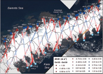
Rate of elevation change along ICESat laser altimetry tracks for the period October 2003-October 2009. Data provided by G. Moholdt (Reference Moholdt, Wouters and GardnerMoholdt and others, 2012). Study glaciers are symbolized according to coast and terminus type as follows: Barents Sea marine-terminating (dark blue circles), Kara Sea marine-terminating (light blue circles), Barents Sea land-terminating (dark red triangles) and Kara Sea land-terminating (light red triangles).

4.1 Glacier retreat

Our data demonstrate that the vast majority (90%) of outlet glaciers on NVZ retreated between 1992 and 2010 (Figs 2 and 5). This concurs with the substantial mass deficit recently reported by Moholdt and others (2012) and highlights the potential contribution of glacier retreat to mass loss from NVZ. The vast majority of retreat occurred on marine-terminating outlets, and losses increased over time (Figs 4 and 5), in contrast to land-terminating glaciers where retreat rates were comparable with frontal position errors. The order-of-magnitude difference in retreat rates between marine- and land-terminating outlets is consistent with previous results from the GrIS (Reference Moon and JoughinMoon and Joughin, 2008;Reference Sole, Payne, Bamber, Nienow and KrabillSole and others, 2008;Reference Pritchard, Arthern, Vaughan and EdwardsPritchard and others, 2009) and Austfonna ice cap, Svalbard (Reference Dowdeswell, Benham and Strozzi Tand HagenDowdeswell and others, 2008). However, it contrasts with the pattern of surface elevation change recently reported for NVZ using ICESat laser altimetry data (Fig. 8), which found no significant difference in frontal thinning rates between marine- and land-terminating glaciers (Reference Gardner, Moholdt, Arendt and WoutersMoholdt and others, 2012). This difference may reflect (1) the spatial coverage of the surface elevation data and/or (2) a delay between terminus retreat and dynamic thinning on marine-terminating outlets. The location of the ICESat tracks results in comparatively sparse data coverage close to the termini of marine-terminating outlets (Fig. 8) where we would expect dynamic thinning in response to recent frontal retreat to be greatest. Consequently, the data may not fully account for near-terminus thinning and may thus underestimate thinning rates on marine-terminating outlets. Alternatively, recent glacier retreat may not yet have initiated dynamic thinning on marine-terminating glaciers, potentially due to slower glacier response times on NVZ in comparison with areas such as the GrIS. If so, recent retreat may result in substantial near-future mass loss from NVZ once the dynamic response begins. This longer-term dynamic component has been highlighted as a potential primary source of future mass loss from the GrIS, where it may account for >75% of 21st-century losses (Reference Price, Payne, Howat and SmithPrice and others, 2011), although dynamic changes may be self-limiting on 200 year timescales (Reference GoelzerGoelzer and others, 2013). Our data therefore suggest that we may be underestimating the contribution of ice dynamics to recent and/or near-future mass losses on NVZ.

4.2. Glacier response to atmospheric and oceanic forcing

4.2.3. Atmospheric forcing

Previous studies have identified a number of different mechanisms by which air temperatures may drive marine-terminating outlet glacier retreat: (1) hydrofracture of crevasses at the terminus/lateral margins (Reference Sohn, Jezek and Van der VeenSohn and others, 1998;Reference AndersenAndersen and others, 2010; Reference Vieli and NickVieli and Nick, 2011); (2) sea-ice melting; and/or (3) enhanced submarine melting due to subglacial meltwater plumes (Reference Sohn, Jezek and Van der VeenSohn and others, 1998; Reference Motyka, Hunter, Echelmeyer and ConnorMotyka and others, 2003, 2011). From visual inspection of satellite imagery, we see no evidence of significant areas of water-filled crevasses during the melt season, and calving generally occurs via small icebergs (<200 m) rather than large tabular icebergs. This indicates that the glacier termini do not have extensive floating sections and will therefore be less vulnerable to full-thickness fracture via meltwater-enhanced crevassing. Moreover, our data show no clear correspondence between variations in air temperature and sea ice (Fig. 6). Instead, sea-ice variability corresponded with changes in SSTs, suggesting that they may be a more significant influence on sea-ice concentrations than air temperatures. Meltwater plumes have been highlighted as a potentially important control on outlet glacier behaviour elsewhere in the Arctic (Reference Motyka, Hunter, Echelmeyer and ConnorMotyka and others, 2003, 2011; Reference Seale, Christoffersen, Mugford and LearyChristoffersen and others, 2011; Reference Seale, Christoffersen, Mugford and LearySeale and others, 2011; Reference StraneoStraneo and others, 2011), and turbid meltwater plumes are evident at the glacier termini. However, very limited oceanographic data are available from NVZ glacial fjords, which precludes a detailed assessment of this mechanism.

Our results show limited correspondence between air temperatures and frontal position variations on NVZ. During the study period, no statistically significant trend was evident in any of our air temperature datasets, in contrast to the acceleration in marine-terminating glacier retreat, and we find no statistical difference in air temperatures before and after the onset of retreat on either coast (Figs 4 and 6). Although previous findings from the GrIS suggest that the response of marine-terminating glaciers to forcing at the terminus is rapid (Reference Vieli and NickVieli and Nick, 2011), we also calculated air temperature trends from the 1950s to the present using reanalysis data, in order to identify any longer-term forcing to which glacier dynamics might be responding. During this time period, we found no significant trend in mean annual or mean summer (June-August) air temperatures in any of the datasets, and mean annual values showed marked interannual and interdecadal variability. Although comparison of meteorological station data with retreat rates is limited by data availability, the pattern of retreat on the Kara Sea coast showed little correspondence to air temperature variations at either meteorological station (Fig. 6). On the Barents Sea coast, the onset of retreat in 2000 followed 2 years of atmospheric warming, but temperatures were equally warm at other points during the study period when retreat rates were lower (Fig. 5). Previous studies have suggested that a longitudinal temperature gradient exists across NVZ (Reference Zeeberg and FormanZeeberg and Forman, 2001), which could potentially contribute to the difference in retreat rates between the Barents and Kara Sea coasts This potential coastal difference cannot be assessed because of lack of data. However, our results provide no evidence for a change in air temperatures that coincided with glacier retreat, suggesting that they are not a primary driver of marine-terminating glacier retreat on NVZ.

Table 3.

Theoretical influence of widening/narrowing of a fjord in the along-flow direction on outlet glacier dynamics

4.3. Fjord width variation

Although mean retreat rates were somewhat higher on the Barents Sea coast than on the Kara Sea coast (Figs 4 and 5), there were large variations in retreat rates between glaciers located on the same coast and even between neighbouring glaciers (Figs 2 and 4), despite being subject to comparable forcing. Together, this evidence suggests that factors specific to each glacier can modulate the glacier’s response to forcing. A number of potential glacier-specific controls have been identified to date, including catchment area, glacier width and basal topography (Reference Carr, Stokes and VieliCarr and others, 2013a). We found no correlation between outlet glacier retreat rate and catchment area (R ² =0.08). However, our data suggest that along-flow variations in fjord width are an important control, and we demonstrate a statistical relationship between fjord width variability and glacier retreat across the study region. We suggest that along-flow width variations may influence retreat rates via two mechanisms: (1) owing to the principle of mass conservation, widening of the fjord would mean that the glacier needs to thin and the surface slope needs to reduce in order to maintain the same ice flux, which would make the ice more vulnerable to thinning and eventually to flotation, thus increasing calving rates and promoting retreat (Reference O’Neel, Pfeffer, Krimmel and MeierO’Neel and others, 2005); and (2) lateral resistive stresses tend to decrease with increasing width, which would reduce resistance to flow and promote further dynamics thinning and retreat (Reference RaymondRaymond, 1996).

In addition to the relationship between retreat rates and width variability, we assessed the relative importance of specific types of width variation (Fig. 3). Based on the hypothesis outlined above, widening of the fjord in the along-flow direction, either rapidly (class I) or gradually (class II), is likely to promote retreat and acceleration (Table 3). Conversely, narrowing of the fjord, either at pinning points (class III) or progressively (class IV), would be expected to reduce retreat rates and ice velocities (Table 3). These changes are likely to occur more rapidly where pinning points are present (classes I and IV) than where changes in fjord width are gradual (classes II and III). Glaciers undergoing minimal along-flow width variation (class VI) will experience limited changes in surface slope, thickness and/or resistive stresses over time, meaning that these factors will have a minimal effect on glacier retreat rates and/or ice velocities.

Fig. 9.

Frontal position of Vil’kitskogo Sev. (VIS) in relation to fjord width perpendicular to the glacier centre line. (a) VIS frontal position over time (colour-coded by year), glacier centre line (black dashed line) and fjord margins as sea level (light grey line). Base image: Landsat scene acquired on 7 July 2010, provided by the USGS Global Visualization Viewer. (b) Fjord width perpendicular to the centre line (blue), in relation to glacier frontal position (red).

Our results demonstrate that rapid retreat was associated with widening fjords and was particularly marked where glaciers retreated from pinning points (Fig. 3). This was exemplified by VIS, located on the Barents Sea coast (Fig. 2), which exhibited the highest mean retreat rate between 1992 and 2010 and the fjord width of which varied by 16% between the most and the least extended frontal positions. Between January 1996 and August 2001, the glacier front occupied a very similar position at a comparatively narrow point of the fjord and its southern margin was attached to a prominent pinning point (Fig. 9, point I). The glacier then retreated rapidly from April 2002, as the southern margin retreated from the pinning point and the front moved into a wider section of the fjord (Fig. 9, point II). Retreat persisted until May 2009, when the fjord narrowed (Fig. 9, point III). This relationship between frontal retreat, pinning points and variations in fjord width is consistent with previous empirical results from Greenland (Reference Warren and GlasserWarren and Glasser, 1992;Reference Carr, Vieli and StokesCarr and others, 2013b) and numerical modelling studies (Reference JamiesonJamieson and others, 2012).

Our results also demonstrate that the glaciers exhibiting the lowest retreat rates have a relatively uniform width along their retreat path and their termini were generally located at narrow points within the fjord (Fig. 3). This is illustrated by Brounova (BRO), which underwent the smallest retreat during the study period. The fjord width varied very little (2.5%) between the minimum and maximum frontal positions, and the terminus occupied a comparatively narrow section of fjord throughout this period (Fig. 10). However, the fjord widens upstream of the current terminus position (Fig. 10), which may facilitate retreat in the future if forcing is sufficient to move the front into this wider section. BRO is located on the Barents Sea coast ~195km north of VIS. Despite this latitudinal difference, sea-ice concentrations at these two glaciers varied by only 4%, whereas the absolute change in frontal position was 48 times greater on VIS than BRO, with VIS retreating by 190ma⁻¹ and BRO advancing by 4 m a⁻¹ during the study period (Fig. 3). A similar pattern is evident along the Barents Sea coast, where the variation in mean monthly sea-ice concentrations was small (SD = 0.67%), but total retreat rate varied markedly, ranging between +4 and –190ma⁻¹ (SD = 47.35 ma⁻¹) (Figs 3 and 5). On the Kara Sea coast, total retreat rates also showed substantial variation (SD = 25.75 m a⁻¹) and variability in sea-ice concentrations was limited, although slightly higher than on the Barents Sea coast (SD = 2.34%). Thus, evidence indicates that there is high variation in retreat rates on both coasts between individual glaciers, but limited variation in forcing, and we suggest that variations in fjord width contribute substantially to these differences.

In addition to the two extreme cases described above, a number of study glaciers experienced retreat only at the central portion of the terminus, while the margins remained on lateral pinning points (Fig. 3). This occurred mainly on the relatively wide outlet glaciers located on the Kara Sea coast, from Moshnyij (MG) northwards (Fig. 2), and is exemplified by the pattern of retreat on MG (Fig. 11). Although detailed bathymetric data are unavailable, topographic maps indicate that the area immediately offshore of these glaciers is shallow and gently sloping, and previous studies suggest that glaciers on the Kara Sea coast terminate in shallow water (Reference KotlyakovKotlyakov, 2006). Owing to the comparatively shallow and wide fjords, ice close to the lateral margins is more likely to be grounded and retreat may therefore be limited to the central portion, where water depths are sufficient to bring the termini close to flotation. Consequently, contemporary forcing may be insufficient to dislodge the glacier termini from their lateral pinning points. This contrasts with fjords located on the Barents Sea coast and further south on the Kara Sea, which are narrower and possibly deeper, as indicated by previous results (Reference KotlyakovKotlyakov, 2006) and bathymetric data from the topographic maps. Narrower fjords are likely to result in a greater contribution of lateral stresses to the force budget, and deeper fjords may allow the terminus to reach near-flotation, which could then facilitate rapid retreat via a series of positive feedbacks once the terminus has moved beyond a pinning point. As a result, differences in fjord geometry may also contribute to the coastal difference in mean retreat rates, as the majority of the wide, shallow fjords are located on the northern Kara Sea coast. A number of the marine-terminating study glaciers also have a portion of their ice front that is land-terminating and this is particularly notable within the northern section of the Kara Sea (Fig. 3). However, this characteristic appears to bear little relationship to glacier retreat rate during the study period (Fig. 3).

Fig. 10.

Frontal position of Brounova (BRO) in relation to fjord width perpendicular to the glacier centre line. (a) BRO frontal position over time (colour-coded by year), glacier centre line (black dashed line) and fjord margins as sea level (light grey line). Base image: Landsat scene acquired on 13 August 2011, provided by the USGS Global Visualization Viewer. (b) Fjord width perpendicular to the centre line (blue), in relation to glacier frontal position (red).

Fig. 11.

Frontal position of Moshnyj(MG) in relation to fjord width perpendicular to the glacier centre line. MG frontal position over time (colour-coded by year), glacier centre line (black dashed line) and fjord margins as sea level (light grey line). Base image: Landsat scene acquired on 13 August 2011, provided by the USGS Global Visualization Viewer.

At present, no data are available on the subglacial topography of NVZ outlet glaciers, and bathymetric information within the fjords is limited. Our results suggest that fjord bathymetry may influence the pattern and magnitude of glacier retreat on the northern section of the Kara Sea coast, where fjords may be comparatively shallow. Retreat rates vary spatially along the fronts of these glaciers (Fig. 11), which may reflect local variations in basal topography and/or bathymetry. Furthermore, rock islands are visible at the calving of a number of the study glaciers (e.g. Krivosheina (KRI) and Chernysheva (CHE)), which may promote retreat as the terminus recedes and ungrounds from these pinning points. It has been suggested that loss of contact with basal pinning points contributed to the dramatic retreat of Jakobs-havn Isbrœ, West Greenland (Reference Thomas, Abdalati, Frederick, Krabill, Manizade and SteffenThomas and others, 2003). Basal topography has been identified as a potentially important control on outlet glacier dynamics in other Arctic regions (Reference Meier and PostMeier and Post, 1987;Reference Nick, Vieli, Howat and JoughinNick and others, 2009; Reference Thomas, Frederick, Krabill, Manizade and MartinThomas and others, 2009) and our results underscore the influence of fjord geometry on glacier retreat rates. Thus, basal topographic and bathymetric data in NVZ are urgently needed to fully understand the factors controlling outlet glacier behaviour and modulating their response to forcing.