


1. Introduction
Ice shelves, floating extensions of grounded ice sheets and glaciers, border much of the Antarctic coastline and are responsible for most of the continent’s ice mass loss. Mass is lost by melting and by iceberg calving, each process accounting for about half the total (Depoorter and others, Reference Depoorter2013, Rignot and others, Reference Rignot, Jacobs, Mouginot and Scheuchl2013). Tabular icebergs, which dominate mass loss by calving (Tournadre and others, Reference Tournadre, Bouhier, Girard-Ardhuin and Rémy2016), separate from ice shelves at through-cutting rifts that form generally transverse to ice flow near the seaward front. Rifts are filled with seawater and often also contain ice mélange, a conglomerate of frozen seawater, shelf-ice and accumulated snow (Swithinbank, Reference Swithinbank1988, p. B26). The rift walls meet at lateral fronts, which appear as rift tips in two-dimensional (2D) plan view. Rifts propagate over timescales that are rapid enough to set them apart as rare examples of geophysical scale fractures for which the entire life cycle might be observed directly (Crary, Reference Crary1961, p. 166).
Fracture propagation is a brittle failure of the material whereby stored elastic potential energy is balanced (released) by splitting the medium (Griffith, Reference Griffith1921). Elastic strain energy may also be dissipated by inelastic deformation (yielding) around the fracture tip. If yielding is small, elastic strain energy is not perturbed appreciably and a linear elastic analysis of the fracture mechanics is appropriate (Tada and others, Reference Tada, Paris and Irwin1985). In linear elastic fracture mechanics (LEFM) theory, stresses in the vicinity of fracture tips are described using stress intensity factors (SIFs) as formulated by Irwin (Lawn and others, Reference Lawn, Lawn Wilshaw and Clarke1993). SIFs correspond to the first terms of a series expansion of the singular stress (or strain) at the sharp fracture front and have the following general formulation
 \begin{equation}
\qquad \qquad \qquad\qquad\qquad\qquad \boldsymbol{\sigma}(r,\theta) = \frac{K}{\sqrt{\pi r}} f(\theta)
\end{equation}
\begin{equation}
\qquad \qquad \qquad\qquad\qquad\qquad \boldsymbol{\sigma}(r,\theta) = \frac{K}{\sqrt{\pi r}} f(\theta)
\end{equation} in which  $\boldsymbol{\sigma} , K, r \,\mathrm{and}\, f(\theta)$ are the stress tensor, SIF, distance to the crack tip and a geometry-dependent function of the angle from the crack plane, respectively (Tada and others, Reference Tada, Paris and Irwin1985). Three SIFs describe three displacement modes at the tip: opening ( $K_\mathrm{I}$), shearing ( $K_\mathrm{II}$) and tearing ( $K_\mathrm{III}$), which correspond to tensile stress across the tip, in-plane shearing and out-of-plane shearing, respectively.
A significant body of work dedicated to the analysis of stresses for idealised reference (or testcase) configurations leads to a catalogue of analytical and often experimentally validated, formulations of  $f(\theta)$ or $f(r,\theta)$ (Tada and others, Reference Tada, Paris and Irwin1985). SIFs may also be inferred using numerical approximation. Numerical approaches are generally one of two types: direct comparison in which computed displacements are compared to an ideal solution (Gupta and others, Reference Gupta, Duarte and Dhankhar2017, Jiménez and Duddu, Reference Jiménez and Duddu2018) or integration approaches based on an energy balance view of the fracture tip (Cherepanov, Reference Cherepanov1967, Rice, Reference Rice1968). Either way, idealised solutions for stress and displacements are required. These are described for plane problems in Williams Reference Williams(1957).
SIFs describe stress and strain conditions at the rift front and are related to the amount of energy available to drive propagation. The theory expects a threshold SIF, sometimes called a fracture toughness value, as a limit beyond which propagation takes place. Empirical studies of laboratory-scale samples yield a range of fracture toughness values, from 0.022 to 0.4 MPa  $\textrm{m}^{1/2}$ (Zhang and others, Reference Zhang, Wang, Han, Li and Wang2023). Similarly, negative SIF values for the opening mode imply the closing of a fracture, allowing for transmission of the compression along the fracture lips, thereby eliminating the tip singularity (Schijve, Reference Schijve2009). Negative mode II or mode III SIFs simply imply an opposing shear orientation. In the ice-shelf system, existing stress fields are expected to relate to opening mode SIF values between zero and the threshold range of toughness values. While this admissible range of SIF values is of general interest here, our specific interest is to analyse how model choices affect the stress and strain conditions at the rift front. Because they describe the elastic solution at a sharp tip, SIFs are ideally suited to this purpose even when they fall outside the physically admissible range. Furthermore, different contributions to SIFs at a rift front may in this way be investigated, regardless of their value, prior to combining contributions, the total of which should be in the physical range.
The spatial dimensions of ice shelves lend themselves to a 2D (plan or cross-section) view of their mechanics. Ice shelves span 100s of km in the horizontal while thicknesses range from ∼1 km at the deepest grounding lines to ∼200 m at calving fronts (Fretwell and others, Reference Fretwell2013). Typical length:thickness ratios are thus around or greater than 1000:1. Many rifts span 10s of km and have length:thickness ratios greater than 100:1. Such scales lend themselves to simplification such as the shallow-shelf, or shelfy-stream, approximation (SSA) of the stress balance for ice-shelf flow (Morland, Reference Morland1987, Muszynski and Birchfield, Reference Muszynski and Birchfield1987, MacAyeal, Reference MacAyeal1989). Plane simplifications may pose some problems in the context of fracture mechanics: the scaling arguments may not hold in the process zone around the tip (Tada and others, Reference Tada, Paris and Irwin1985) and singular stress patterns due to the intersection of the rift front and the upper or lower shelf surface may be important (Bazant and Estenssoro, Reference Bazant and Estenssoro1979). Additionally, the imbalance between the ice and ocean (or ocean + mélange) overburden pressures at vertical faces of a rift has an out-of-plane dependence (Reeh, Reference Reeh1968) that cannot be represented in plane. Furthermore, incompressibility of viscous deformation is required to establish the SSA and this conflicts with laboratory observations of the elastic case (Schulson and Duval, Reference Schulson and Duval2009). Nevertheless, 2D representations of fracture mechanics are desirable for glaciological problems because they lend themselves to integration with common 2D approximations (as in Smith, Reference Smith1976, van der Veen, Reference van der Veen1998, Hulbe and others, Reference Hulbe, LeDoux and Cruikshank2010, Plate and others, Reference Plate, Gross, Humbert and Müller2012, Lipovsky, Reference Lipovsky2020).
The first applications of LEFM investigated vertically propagating crevasses (Smith, Reference Smith1976, van der Veen, Reference van der Veen1998) using the 2D assumption of plane strain conditions and crevasse-perpendicular stresses inferred from observed viscous strain rates. Hulbe and others Reference Hulbe, LeDoux and Cruikshank(2010) apply the same conceptual view to evaluate stresses in the vicinity of laterally propagating rifts using a boundary element model. Plate and others (Reference Plate, Gross, Humbert and Müller2012) use a configurational force approach to impose stresses from a viscous flow model onto a plane stress approximation of an elastic ice-shelf model. More recently, Lipovsky Reference Lipovsky(2020) solved a 3D elastic ice-shelf problem for a ‘perturbation’ stress field made by subtracting the glaciostatic overburden from the total Cauchy stress tensor. In this case, stresses are calculated from boundary conditions using the elastic constitutive relationship for all of a characteristic testcase shelf. A depth relationship for SIFs obtained from a 3D model is fit and then used when interpreting results from a 2D plane strain representation.
Damage approaches, particularly anisotropic damage mechanics, have also been used to represent crevasses and rifts. For example, Sun and others Reference Sun, Duddu and Hirshikesh(2021) and Clayton and others Reference Clayton, Duddu, Siegert and Martínez-Pañeda(2022) use this theoretical framework to predict crevasse penetration depth using fracture energy functionals in the damage approach to achieve LEFM results. In the case of laterally propagating rifts, Huth and others Reference Huth, Duddu, Smith and Sergienko(2023) apply anisotropic damage evolution in a viscous SSA with threshold stress criteria to simulate both propagation and rift widening. The formulation accounts for mélange within rifts but uses only a viscous constitutive relationship despite the fast rate of change.
Across all of the preceding examples, and others (for example, De Rydt and others, Reference De Rydt, Gudmundsson, Nagler and Wuite2019, Wang and others, Reference Wang2022), relatively little has been written about the nature of the elastic plane problem (plane stress vs plane strain), the application of stresses derived using one simplification to a problem solved using the other or the relationship between the 2D problem being solved and the 3D system it approximates. Huth and others Reference Huth, Duddu, Smith and Sergienko(2023) include an extension of the plane problem to the vertical effects of water pressure and Lipovsky Reference Lipovsky(2020) provides 3D to 2D comparisons for particular rift-shelf configurations.
The aim of the present contribution is to establish an appropriate 2D approximation for simulating the elastic problem, compatible with the shallow-shelf approach for the viscous problem. First, a plane stress approximation is shown to be appropriate for the elastic problem as it relates to rift propagation. As noted above, 2D representations are incomplete at domain boundaries. Rifts are such boundaries and we therefore verify the effects of incorporating them into a 2D, rather than 3D, model. This is accomplished by comparing 2D and 3D models focused on vertical variations in rift wall loading due to infilling ocean water and its effects on 2D and 3D SIFs. Open-source FEM models are used in this work.
2. 2D representation of ice shelves
Scaling arguments and perturbation series expansions have long been used to achieve useful simplifications to the governing equations for viscous ice sheet and ice-shelf flow (Morland and Johnson, Reference Morland and Johnson1980, Shoemaker and Morland, Reference Shoemaker and Morland1984, McMeeking and Johnson, Reference McMeeking and Johnson1986). The widely used SSA, in which deviatoric stresses are associated with viscous deformation, is derived for cases in which basal shear stress is zero (the ice-shelf case) or very small (the shelfy-stream case) (Morland, Reference Morland1987, Muszynski and Birchfield, Reference Muszynski and Birchfield1987, MacAyeal, Reference MacAyeal1989). Here, the shallow-shelf problem is developed using the total stress tensor as far as possible, so that the result is agnostic to constitutive relationship and thus compatible with the elastic deformation.
2.1. Ice-shelf boundary value problem
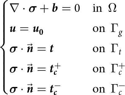
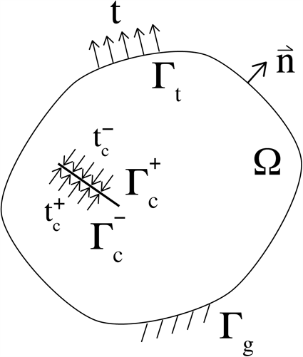
Ultimately, ice deformation is inferred from either the displacement (elastic) or velocity (viscous) solution to the same boundary value problem (BVP), represented here in a traditional potato-shape schematic (Fig. 1). The strong form of the problem is given by the momentum equilibrium equation and boundary conditions
 \begin{equation}
\begin{cases}
\nabla \cdot \boldsymbol{\sigma }+ \boldsymbol{b} = 0 &\text{in} \ \ \Omega \\
\boldsymbol{u} = \boldsymbol{u_0} &\text{on} \ \ \Gamma_{g} \\
\boldsymbol{\sigma} \cdot \vec{\boldsymbol{n}} = \boldsymbol{t} \quad \quad &\text{on} \ \ \Gamma_{t}\\
\boldsymbol{\sigma } \cdot \vec{\boldsymbol{n}} = \boldsymbol{t_{c}^{+}} &\text{on} \ \ \Gamma_{c}^{+}\\
\boldsymbol{\sigma } \cdot \vec{\boldsymbol{n}} = \boldsymbol{t_{c}^{-}} &\text{on} \ \ \Gamma_{c}^{-}\\
\end{cases}
\end{equation}
\begin{equation}
\begin{cases}
\nabla \cdot \boldsymbol{\sigma }+ \boldsymbol{b} = 0 &\text{in} \ \ \Omega \\
\boldsymbol{u} = \boldsymbol{u_0} &\text{on} \ \ \Gamma_{g} \\
\boldsymbol{\sigma} \cdot \vec{\boldsymbol{n}} = \boldsymbol{t} \quad \quad &\text{on} \ \ \Gamma_{t}\\
\boldsymbol{\sigma } \cdot \vec{\boldsymbol{n}} = \boldsymbol{t_{c}^{+}} &\text{on} \ \ \Gamma_{c}^{+}\\
\boldsymbol{\sigma } \cdot \vec{\boldsymbol{n}} = \boldsymbol{t_{c}^{-}} &\text{on} \ \ \Gamma_{c}^{-}\\
\end{cases}
\end{equation} in which σ is the Cauchy stress tensor; b represents the body forces; Ω is the BVP domain; u represents the displacement field and  $\boldsymbol{u_0}$ are prescribed or initial displacements; $\Gamma_t$, $\Gamma_c^{+}$, $\Gamma_c^{-}$ and $\Gamma_g$ are boundaries to the domain; t, $\boldsymbol{t_c^{+}}$ and $\boldsymbol{t_c^{-}}$ are boundary tractions and $\vec{\boldsymbol{n}}$ is the unit normal to any of the domain boundaries. The boundaries $\Gamma_c^{+}$ and $\Gamma_c^{-}$ correspond opposing rift walls and in this work will be assumed to be loaded by equal and opposing tractions, i.e. $\boldsymbol{t_c}^{+} = - \boldsymbol{t_c}^{-}$. Boundaries that are exposed to the atmosphere have zero normal or shear stress conditions.
Boundary value problem (BVP) in a global reference frame. The domain over which the BVP applies is Ω. The variable t is used to denote tractions acting on boundaries and c a rift. Boundaries to the domain, Γ, have a normal  $\vec{\boldsymbol{n}}$ and subscripts t, c and g to describe boundaries: subject to traction, part of a rift or fixed. In the case of the boundaries defined by a rift, $\Gamma_{c}$, the superscripts + and − are used to distinguish between the two rift surfaces.
2.2. Constitutive relationships for modelling ice
The constitutive relation for the domain Ω must be representative of natural ice and describe the deformation behaviour—elastic, viscous or both—targeted by the model. The Cauchy stress σ, strain ϵ and strain-rate  $\dot{\epsilon}$ are second order symmetrical tensors (e.g.
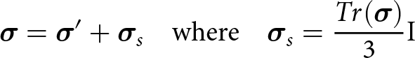
Coman, Reference Coman2020). The stress tensor σ can be separated into deviatoric stress causing distortion deformation and spherical (or non-deviatoric) stress causing a volume deformation
$\dot{\epsilon}$ are second order symmetrical tensors (e.g.
Coman, Reference Coman2020). The stress tensor σ can be separated into deviatoric stress causing distortion deformation and spherical (or non-deviatoric) stress causing a volume deformation
 \begin{equation}
\boldsymbol{\sigma} = \boldsymbol{\sigma}' + \boldsymbol{\sigma}_{s} \quad \text{where} \quad \boldsymbol{\sigma}_{s} = \frac{Tr(\boldsymbol{\sigma})}{3} \boldsymbol{\text{I}}
\end{equation}
\begin{equation}
\boldsymbol{\sigma} = \boldsymbol{\sigma}' + \boldsymbol{\sigma}_{s} \quad \text{where} \quad \boldsymbol{\sigma}_{s} = \frac{Tr(\boldsymbol{\sigma})}{3} \boldsymbol{\text{I}}
\end{equation} and where  $\boldsymbol{\sigma}'$ is the deviatoric stress, $\boldsymbol{\sigma}_{s}$ the spherical stress and $\boldsymbol{\text{I}}$ the $3\times3$ identity matrix.
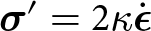
Nye’s generalisation of the Glen flow law (Nye, Reference Nye1952) provides the constitutive relationship between strain rate  $\dot{\boldsymbol{\epsilon}}$ and deviatoric stress $\boldsymbol{\sigma}'$,
 \begin{equation}
\boldsymbol{\sigma}' = 2\kappa\dot{\boldsymbol{\epsilon}}
\end{equation}
\begin{equation}
\boldsymbol{\sigma}' = 2\kappa\dot{\boldsymbol{\epsilon}}
\end{equation} for viscous deformation in the case of incompressibility. The viscosity κ depends on  $\dot{\boldsymbol{\epsilon}}$ and on temperature T such that
 \begin{equation}
\kappa = A(T)\dot{\epsilon}_{II}^{\frac{n}{n-1}}
\end{equation}
\begin{equation}
\kappa = A(T)\dot{\epsilon}_{II}^{\frac{n}{n-1}}
\end{equation} in which the empirically derived rate factor function and exponent are A(T) and n, respectively. Generally, an exponent n = 3 is used. The effective strain rate  $\dot{\epsilon}_{II}$ is given by
 \begin{equation}
\dot{\epsilon}_{II} = \sqrt{\frac{1}{2} \dot{\epsilon}_{ij} \dot{\epsilon}_{ij}}.
\end{equation}
\begin{equation}
\dot{\epsilon}_{II} = \sqrt{\frac{1}{2} \dot{\epsilon}_{ij} \dot{\epsilon}_{ij}}.
\end{equation} Strain rate and strain are related by the derivative  $\dot{\boldsymbol{\epsilon}} = \partial \boldsymbol{\epsilon}/{\partial t}$. The focus of this work is to provide a 2D approximation for the steady-state elastic BVP problem on short timescales. However, the steady-state long timescale viscous BVP is required to obtain the initial loading condition of prior to propagation. Due to the two timescales being considered independently, the link between strain and strain rate is not used here. The constitutive relationship for elastic deformation, considered here to be linear and isotropic (Sergienko, Reference Sergienko2010, and citations within), is
 \begin{equation}
\boldsymbol{\sigma} = \lambda \text{Tr}( \boldsymbol{\epsilon}) \textbf{I}+2\mu{\boldsymbol{\epsilon}}
\end{equation}
\begin{equation}
\boldsymbol{\sigma} = \lambda \text{Tr}( \boldsymbol{\epsilon}) \textbf{I}+2\mu{\boldsymbol{\epsilon}}
\end{equation}in which (Lamé) coefficients λ and µ are
 \begin{equation}
\lambda = \frac{E\nu}{(1+\nu)(1-2\nu)}, \quad \mu = \frac{E}{2(1 + \nu)}
\end{equation}
\begin{equation}
\lambda = \frac{E\nu}{(1+\nu)(1-2\nu)}, \quad \mu = \frac{E}{2(1 + \nu)}
\end{equation}written in terms of (Young’s) modulus of elasticity E and (Poisson’s) coefficient ν expressing the ratio between transverse contraction and longitudinal extension. The elastic constitutive relation can also be formulated so as to separate deviatoric and spherical strain
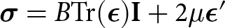 \begin{equation}
\boldsymbol{\sigma} = B \text{Tr}(\boldsymbol{\epsilon}) \textbf{I}+2\mu{\boldsymbol{\epsilon}'}
\end{equation}
\begin{equation}
\boldsymbol{\sigma} = B \text{Tr}(\boldsymbol{\epsilon}) \textbf{I}+2\mu{\boldsymbol{\epsilon}'}
\end{equation} in which  $\epsilon'$ is the deviatoric part of the strain and B is the bulk modulus. The bulk modulus relates to both Lamé constants
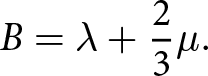 \begin{equation}
B = \lambda+\frac{2}{3}\mu.
\end{equation}
\begin{equation}
B = \lambda+\frac{2}{3}\mu.
\end{equation}2.3. 3D description of the ice shelf
The general description of the ice-shelf continuum for either viscous or elastic constitutive relationships is given by equilibrium equations for the domain in (2). Adopting a Cartesian coordinate system, the equilibrium equation for each coordinate is
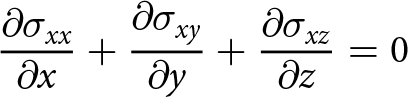 \begin{align}
{\frac{\partial{\sigma_{xx}}}{\partial{x}}}+ {\frac{\partial{\sigma_{xy}}}{\partial{y}}} + {\frac{\partial{\sigma_{xz}}}{\partial{z}}} &= 0
\end{align}
\begin{align}
{\frac{\partial{\sigma_{xx}}}{\partial{x}}}+ {\frac{\partial{\sigma_{xy}}}{\partial{y}}} + {\frac{\partial{\sigma_{xz}}}{\partial{z}}} &= 0
\end{align}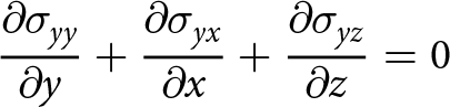 \begin{align}
{\frac{\partial{\sigma_{yy}}}{\partial{y}}}+ {\frac{\partial{\sigma_{yx}}}{\partial{x}}} + {\frac{\partial{\sigma_{yz}}}{\partial{z}}} &= 0
\end{align}
\begin{align}
{\frac{\partial{\sigma_{yy}}}{\partial{y}}}+ {\frac{\partial{\sigma_{yx}}}{\partial{x}}} + {\frac{\partial{\sigma_{yz}}}{\partial{z}}} &= 0
\end{align}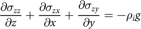 \begin{align}
{\frac{\partial{\sigma_{zz}}}{\partial{z}}}+ {\frac{\partial{\sigma_{zx}}}{\partial{x}}} + {\frac{\partial{\sigma_{zy}}}{\partial{y}}} &= -\rho_i g
\end{align}
\begin{align}
{\frac{\partial{\sigma_{zz}}}{\partial{z}}}+ {\frac{\partial{\sigma_{zx}}}{\partial{x}}} + {\frac{\partial{\sigma_{zy}}}{\partial{y}}} &= -\rho_i g
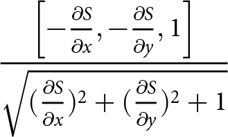
\end{align} where ρi is the density of the ice and g is the acceleration due to gravity. Boundary conditions for the upper surface  $S(x,y)$, the underside $B(x,y)$ and the shelf front $F(x,y,z)$ require a set of unit normal vectors
 \begin{align}
\frac{\left[-{\frac{\partial{S}}{\partial{x}}},-{\frac{\partial{S}}{\partial{y}}},1\right]}{\sqrt{({\frac{\partial{S}}{\partial{x}}})^2+({\frac{\partial{S}}{\partial{y}}})^2+1}}
\end{align}
\begin{align}
\frac{\left[-{\frac{\partial{S}}{\partial{x}}},-{\frac{\partial{S}}{\partial{y}}},1\right]}{\sqrt{({\frac{\partial{S}}{\partial{x}}})^2+({\frac{\partial{S}}{\partial{y}}})^2+1}}
\end{align}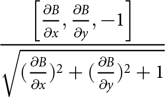 \begin{align}
\frac{\left[{\frac{\partial{B}}{\partial{x}}},{\frac{\partial{B}}{\partial{y}}},-1\right]}{\sqrt{({\frac{\partial{B}}{\partial{x}}})^2+({\frac{\partial{B}}{\partial{y}}})^2+1}}
\end{align}
\begin{align}
\frac{\left[{\frac{\partial{B}}{\partial{x}}},{\frac{\partial{B}}{\partial{y}}},-1\right]}{\sqrt{({\frac{\partial{B}}{\partial{x}}})^2+({\frac{\partial{B}}{\partial{y}}})^2+1}}
\end{align}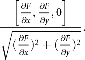 \begin{align}
\frac{\left[{\frac{\partial{F}}{\partial{x}}},{\frac{\partial{F}}{\partial{y}}},0\right]}{\sqrt{({\frac{\partial{F}}{\partial{x}}})^2+({\frac{\partial{F}}{\partial{y}}})^2}}.
\end{align}
\begin{align}
\frac{\left[{\frac{\partial{F}}{\partial{x}}},{\frac{\partial{F}}{\partial{y}}},0\right]}{\sqrt{({\frac{\partial{F}}{\partial{x}}})^2+({\frac{\partial{F}}{\partial{y}}})^2}}.
\end{align} The front is assumed to be perfectly vertical, making the  $\vec{\boldsymbol{z}}$ term in unit normal vector in Eqn (12c) equal to zero.
Boundaries exposed to the atmosphere experience zero pressure (the atmospheric pressure is negligible) and submerged boundaries experience depth-dependent water pressure. Consequently, at the upper surface
 \begin{align}
-\sigma_{xx}\big|_{\scriptscriptstyle S}{\frac{\partial{S}}{\partial{x}}} -\sigma_{xy}\big|_{\scriptscriptstyle S}{\frac{\partial{S}}{\partial{y}}}+ \sigma_{xz}\big|_{\scriptscriptstyle S} = 0
\end{align}
\begin{align}
-\sigma_{xx}\big|_{\scriptscriptstyle S}{\frac{\partial{S}}{\partial{x}}} -\sigma_{xy}\big|_{\scriptscriptstyle S}{\frac{\partial{S}}{\partial{y}}}+ \sigma_{xz}\big|_{\scriptscriptstyle S} = 0
\end{align}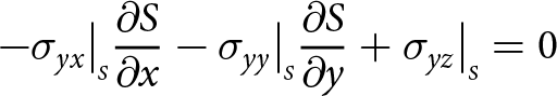 \begin{align}
-\sigma_{yx}\big|_{\scriptscriptstyle S}{\frac{\partial{S}}{\partial{x}}} -\sigma_{yy}\big|_{\scriptscriptstyle S}{\frac{\partial{S}}{\partial{y}}}+ \sigma_{yz}\big|_{\scriptscriptstyle S} = 0
\end{align}
\begin{align}
-\sigma_{yx}\big|_{\scriptscriptstyle S}{\frac{\partial{S}}{\partial{x}}} -\sigma_{yy}\big|_{\scriptscriptstyle S}{\frac{\partial{S}}{\partial{y}}}+ \sigma_{yz}\big|_{\scriptscriptstyle S} = 0
\end{align}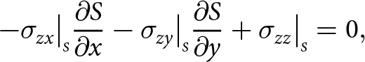 \begin{align}
-\sigma_{zx}\big|_{\scriptscriptstyle S}{\frac{\partial{S}}{\partial{x}}} -\sigma_{zy}\big|_{\scriptscriptstyle S}{\frac{\partial{S}}{\partial{y}}}+ \sigma_{zz}\big|_{\scriptscriptstyle S} = 0,
\end{align}
\begin{align}
-\sigma_{zx}\big|_{\scriptscriptstyle S}{\frac{\partial{S}}{\partial{x}}} -\sigma_{zy}\big|_{\scriptscriptstyle S}{\frac{\partial{S}}{\partial{y}}}+ \sigma_{zz}\big|_{\scriptscriptstyle S} = 0,
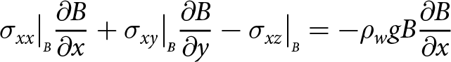
\end{align}at the base
 \begin{align}
\sigma_{xx}\big|_{\scriptscriptstyle B}{\frac{\partial{B}}{\partial{x}}} +\sigma_{xy}\big|_{\scriptscriptstyle B}{\frac{\partial{B}}{\partial{y}}}- \sigma_{xz}\big|_{\scriptscriptstyle B} = -\rho_{w} g B {\frac{\partial{B}}{\partial{x}}}
\end{align}
\begin{align}
\sigma_{xx}\big|_{\scriptscriptstyle B}{\frac{\partial{B}}{\partial{x}}} +\sigma_{xy}\big|_{\scriptscriptstyle B}{\frac{\partial{B}}{\partial{y}}}- \sigma_{xz}\big|_{\scriptscriptstyle B} = -\rho_{w} g B {\frac{\partial{B}}{\partial{x}}}
\end{align}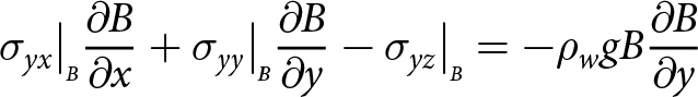 \begin{align}
\sigma_{yx}\big|_{\scriptscriptstyle B}{\frac{\partial{B}}{\partial{x}}} +\sigma_{yy}\big|_{\scriptscriptstyle B}{\frac{\partial{B}}{\partial{y}}}- \sigma_{yz}\big|_{\scriptscriptstyle B} = -\rho_{w} g B {\frac{\partial{B}}{\partial{y}}}
\end{align}
\begin{align}
\sigma_{yx}\big|_{\scriptscriptstyle B}{\frac{\partial{B}}{\partial{x}}} +\sigma_{yy}\big|_{\scriptscriptstyle B}{\frac{\partial{B}}{\partial{y}}}- \sigma_{yz}\big|_{\scriptscriptstyle B} = -\rho_{w} g B {\frac{\partial{B}}{\partial{y}}}
\end{align}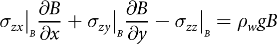 \begin{align}
\sigma_{zx}\big|_{\scriptscriptstyle B}{\frac{\partial{B}}{\partial{x}}} +\sigma_{zy}\big|_{\scriptscriptstyle B}{\frac{\partial{B}}{\partial{y}}} -\sigma_{zz}\big|_{\scriptscriptstyle B} =\rho_{w} g B
\end{align}
\begin{align}
\sigma_{zx}\big|_{\scriptscriptstyle B}{\frac{\partial{B}}{\partial{x}}} +\sigma_{zy}\big|_{\scriptscriptstyle B}{\frac{\partial{B}}{\partial{y}}} -\sigma_{zz}\big|_{\scriptscriptstyle B} =\rho_{w} g B
\end{align}and finally, at the front
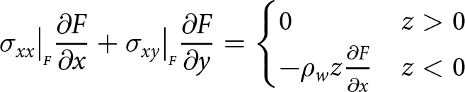 \begin{align}
\sigma_{xx}\big|_{\scriptscriptstyle F}{\frac{\partial{F}}{\partial{x}}} +\sigma_{xy}\big|_{\scriptscriptstyle F}{\frac{\partial{F}}{\partial{y}}} =
\begin{cases}
0 & z \gt 0 \\
-\rho_{w} z {\frac{\partial{F}}{\partial{x}}} & z \lt 0
\end{cases}
\end{align}
\begin{align}
\sigma_{xx}\big|_{\scriptscriptstyle F}{\frac{\partial{F}}{\partial{x}}} +\sigma_{xy}\big|_{\scriptscriptstyle F}{\frac{\partial{F}}{\partial{y}}} =
\begin{cases}
0 & z \gt 0 \\
-\rho_{w} z {\frac{\partial{F}}{\partial{x}}} & z \lt 0
\end{cases}
\end{align}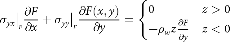 \begin{align}
\sigma_{yx}\big|_{\scriptscriptstyle F}{\frac{\partial{F}}{\partial{x}}} +\sigma_{yy}\big|_{\scriptscriptstyle F}{\frac{\partial{F(x,y)}}{\partial{y}}} =
\begin{cases}
0 & z \gt 0 \\
-\rho_{w} z {\frac{\partial{F}}{\partial{y}}} & z \lt 0
\end{cases}
\end{align}
\begin{align}
\sigma_{yx}\big|_{\scriptscriptstyle F}{\frac{\partial{F}}{\partial{x}}} +\sigma_{yy}\big|_{\scriptscriptstyle F}{\frac{\partial{F(x,y)}}{\partial{y}}} =
\begin{cases}
0 & z \gt 0 \\
-\rho_{w} z {\frac{\partial{F}}{\partial{y}}} & z \lt 0
\end{cases}
\end{align}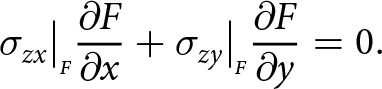 \begin{align}
\sigma_{zx}\big|_{\scriptscriptstyle F}{\frac{\partial{F}}{\partial{x}}} +\sigma_{zy}\big|_{\scriptscriptstyle F}{\frac{\partial{F}}{\partial{y}}} = 0.
\end{align}
\begin{align}
\sigma_{zx}\big|_{\scriptscriptstyle F}{\frac{\partial{F}}{\partial{x}}} +\sigma_{zy}\big|_{\scriptscriptstyle F}{\frac{\partial{F}}{\partial{y}}} = 0.
\end{align}2.4. Non-dimensional scaling of the problem
Non-dimensionalisation, or scaling, is a change of variables used to facilitate simplifications to the governing equations. For example, any model length x in the  $\vec{\boldsymbol{x}}$ direction is scaled as $\tilde{x}=\frac{x}{L}$ in which L is a characteristic length of an ice shelf. Similarly, any model length z in the $\vec{\boldsymbol{z}}$ direction is scaled with the characteristic thickness H. The ratio δ of characteristic ice-shelf thickness H to characteristic ice-shelf extent L is small and used for the perturbation series expansion in the next subsection.
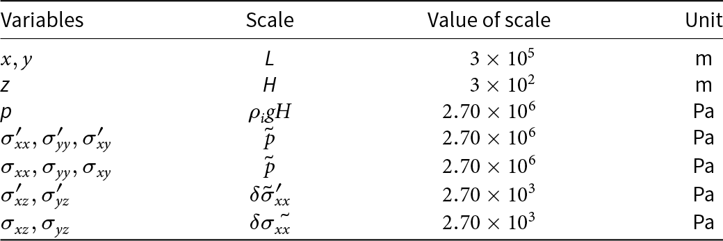
Material properties are taken to be constant and used to infer sensible scaling for variables (Table 1). In this case,  $E = 9.6\times10^9$ and ν = 0.33. Mean densities of $\rho_i = 917 \,\text{kg m}^{-3}$ and $\rho_w = 1023 \,\text{kg m}^{-3}$ are used for ice and ocean water, respectively (Cuffey and Paterson, Reference Cuffey and Paterson2010). In the case of the elastic problem, changes in density due to deformation are neglected for linear analysis (see, for example,
Martinec, Reference Martinec2019).
$\rho_w = 1023 \,\text{kg m}^{-3}$ are used for ice and ocean water, respectively (Cuffey and Paterson, Reference Cuffey and Paterson2010). In the case of the elastic problem, changes in density due to deformation are neglected for linear analysis (see, for example,
Martinec, Reference Martinec2019).
Variables and characteristic scales for the ice-shelf problem. From the characteristic length scales of the problem geometry,  $\delta = 10^{-3}$ is then used for $\sigma'_{xz},\sigma'_{yz}$ and $\sigma_{xz},\sigma_{yz}$
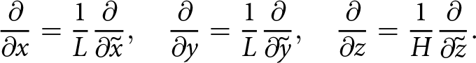
Differentiating with respect to scaled variables is as follows:
 \begin{equation}
\frac{\partial}{\partial{x}}=\frac{1}{L}\frac{\partial}{\partial{\tilde{x}}}, \quad \frac{\partial}{\partial{y}}=\frac{1}{L}\frac{\partial}{\partial{\tilde{y}}}, \quad \frac{\partial}{\partial{z}}=\frac{1}{H}\frac{\partial}{\partial{\tilde{z}}}.
\end{equation}
\begin{equation}
\frac{\partial}{\partial{x}}=\frac{1}{L}\frac{\partial}{\partial{\tilde{x}}}, \quad \frac{\partial}{\partial{y}}=\frac{1}{L}\frac{\partial}{\partial{\tilde{y}}}, \quad \frac{\partial}{\partial{z}}=\frac{1}{H}\frac{\partial}{\partial{\tilde{z}}}.
\end{equation}The dimensionless equations of conservation of momentum, Eqn (2) or (11), become
 \begin{align}
{\frac{\partial{\tilde{\sigma}_{xx}}}{\partial{\tilde{x}}}}+ {\frac{\partial{\tilde{\sigma}_{xy}}}{\partial{\tilde{y}}}} + {\frac{\partial{\tilde{\sigma}_{xz}}}{\partial{\tilde{z}}}} &= 0
\end{align}
\begin{align}
{\frac{\partial{\tilde{\sigma}_{xx}}}{\partial{\tilde{x}}}}+ {\frac{\partial{\tilde{\sigma}_{xy}}}{\partial{\tilde{y}}}} + {\frac{\partial{\tilde{\sigma}_{xz}}}{\partial{\tilde{z}}}} &= 0
\end{align}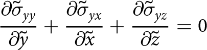 \begin{align}
{\frac{\partial{\tilde{\sigma}_{yy}}}{\partial{\tilde{y}}}}+ {\frac{\partial{\tilde{\sigma}_{yx}}}{\partial{\tilde{x}}}} + {\frac{\partial{\tilde{\sigma}_{yz}}}{\partial{\tilde{z}}}} &= 0
\end{align}
\begin{align}
{\frac{\partial{\tilde{\sigma}_{yy}}}{\partial{\tilde{y}}}}+ {\frac{\partial{\tilde{\sigma}_{yx}}}{\partial{\tilde{x}}}} + {\frac{\partial{\tilde{\sigma}_{yz}}}{\partial{\tilde{z}}}} &= 0
\end{align}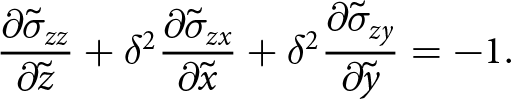 \begin{align}
{\frac{\partial{\tilde{\sigma}_{zz}}}{\partial{\tilde{z}}}}+ \delta^2 {\frac{\partial{\tilde{\sigma}_{zx}}}{\partial{\tilde{x}}}} + \delta^2 {\frac{\partial{\tilde{\sigma}_{zy}}}{\partial{\tilde{y}}}} &= - 1.
\end{align}
\begin{align}
{\frac{\partial{\tilde{\sigma}_{zz}}}{\partial{\tilde{z}}}}+ \delta^2 {\frac{\partial{\tilde{\sigma}_{zx}}}{\partial{\tilde{x}}}} + \delta^2 {\frac{\partial{\tilde{\sigma}_{zy}}}{\partial{\tilde{y}}}} &= - 1.
\end{align}The conditions at the shelf boundaries, Eqns (13)–(15) are presented in dimensionless form in Appendix 6.1.
2.5. Perturbation series expansion
A perturbation series expansion is used to simplify the governing equations using the problem scaling which leads to a small ratio δ, where
 \begin{equation}
\delta = \frac{H}{L} \lt \lt 1.
\end{equation}
\begin{equation}
\delta = \frac{H}{L} \lt \lt 1.
\end{equation}The problem variables, for example σ, are expanded in a power series in δ,
 \begin{equation}
\boldsymbol{\tilde{\sigma}} = \sum^{\infty}_{i=0}{\delta^{i}\boldsymbol{\tilde{\sigma}}_{(i)}}
\end{equation}
\begin{equation}
\boldsymbol{\tilde{\sigma}} = \sum^{\infty}_{i=0}{\delta^{i}\boldsymbol{\tilde{\sigma}}_{(i)}}
\end{equation}and then the zeroth-order terms of δ are gathered to form a scaled approximation (Weis, Reference Weis2001, Ahlkrona and others, Reference Ahlkrona, Kirchner and Lötstedt2013). Using this approach, Eqn (17) becomes
 \begin{align}
{\frac{\partial{\tilde{\sigma}_{xx}}}{\partial{\tilde{x}}}}+ {\frac{\partial{\tilde{\sigma}_{xy}}}{\partial{\tilde{y}}}} + {\frac{\partial{\tilde{\sigma}_{xz}}}{\partial{\tilde{z}}}} &= 0
\end{align}
\begin{align}
{\frac{\partial{\tilde{\sigma}_{xx}}}{\partial{\tilde{x}}}}+ {\frac{\partial{\tilde{\sigma}_{xy}}}{\partial{\tilde{y}}}} + {\frac{\partial{\tilde{\sigma}_{xz}}}{\partial{\tilde{z}}}} &= 0
\end{align} \begin{align}
{\frac{\partial{\tilde{\sigma}_{yy}}}{\partial{\tilde{y}}}}+ {\frac{\partial{\tilde{\sigma}_{yx}}}{\partial{\tilde{x}}}} + {\frac{\partial{\tilde{\sigma}_{yz}}}{\partial{\tilde{z}}}} &= 0
\end{align}
\begin{align}
{\frac{\partial{\tilde{\sigma}_{yy}}}{\partial{\tilde{y}}}}+ {\frac{\partial{\tilde{\sigma}_{yx}}}{\partial{\tilde{x}}}} + {\frac{\partial{\tilde{\sigma}_{yz}}}{\partial{\tilde{z}}}} &= 0
\end{align} \begin{align}
{\frac{\partial{\tilde{\sigma}_{zz}}}{\partial{\tilde{z}}}} &= - 1.
\end{align}
\begin{align}
{\frac{\partial{\tilde{\sigma}_{zz}}}{\partial{\tilde{z}}}} &= - 1.
\end{align}The zeroth-order conditions on the upper, base and front surfaces are detailed in Appendix 6.2.
2.6. Vertical integration
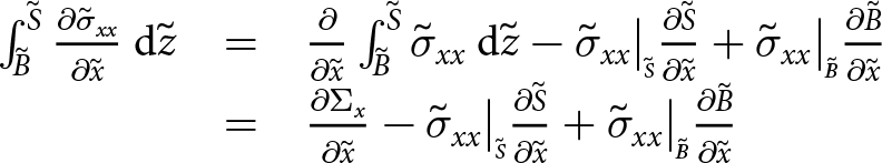
Vertical or depth integration of the governing equations then reduces the problem to two dimensions. This is demonstrated for all of the different components of the first line in Eqn (20). Depth integration of  $\partial{\tilde{\sigma}_{xx}}/\partial{\tilde{x}}$ is
 \begin{equation}
\begin{array}{rcl}
\int_{{\tilde{B}}}^{{\tilde{S}}} {{\frac{\partial{\tilde{\sigma}_{xx}}}{\partial{\tilde{x}}}}} \: \mathrm{d}{\tilde{z}} &=& \frac{\partial}{\partial{\tilde{x}}} \int_{{\tilde{B}}}^{{\tilde{S}}} {\tilde{\sigma}_{xx}} \: \mathrm{d}{\tilde{z}} - \tilde{\sigma}_{xx}\big|_{\scriptscriptstyle \tilde{S}} {\frac{\partial{\tilde{S}}}{\partial{\tilde{x}}}} + \tilde{\sigma}_{xx}\big|_{\scriptscriptstyle \tilde{B}}{\frac{\partial{\tilde{B}}}{\partial{\tilde{x}}}} \\
&=& {\frac{\partial{\Sigma_{x}}}{\partial{\tilde{x}}}} - \tilde{\sigma}_{xx}\big|_{\scriptscriptstyle \tilde{S}}{\frac{\partial{\tilde{S}}}{\partial{\tilde{x}}}} + \tilde{\sigma}_{xx}\big|_{\scriptscriptstyle \tilde{B}}{\frac{\partial{\tilde{B}}}{\partial{\tilde{x}}}}
\end{array}
\end{equation}
\begin{equation}
\begin{array}{rcl}
\int_{{\tilde{B}}}^{{\tilde{S}}} {{\frac{\partial{\tilde{\sigma}_{xx}}}{\partial{\tilde{x}}}}} \: \mathrm{d}{\tilde{z}} &=& \frac{\partial}{\partial{\tilde{x}}} \int_{{\tilde{B}}}^{{\tilde{S}}} {\tilde{\sigma}_{xx}} \: \mathrm{d}{\tilde{z}} - \tilde{\sigma}_{xx}\big|_{\scriptscriptstyle \tilde{S}} {\frac{\partial{\tilde{S}}}{\partial{\tilde{x}}}} + \tilde{\sigma}_{xx}\big|_{\scriptscriptstyle \tilde{B}}{\frac{\partial{\tilde{B}}}{\partial{\tilde{x}}}} \\
&=& {\frac{\partial{\Sigma_{x}}}{\partial{\tilde{x}}}} - \tilde{\sigma}_{xx}\big|_{\scriptscriptstyle \tilde{S}}{\frac{\partial{\tilde{S}}}{\partial{\tilde{x}}}} + \tilde{\sigma}_{xx}\big|_{\scriptscriptstyle \tilde{B}}{\frac{\partial{\tilde{B}}}{\partial{\tilde{x}}}}
\end{array}
\end{equation} in which  $\Sigma_{x}$ represents the depth integration of $\tilde{\sigma}_{xx}$ through the shelf thickness. Depth integration of
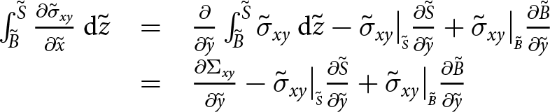
  $\partial{\tilde{\sigma}_{xy}}/\partial{\tilde{y}}$ is
 \begin{equation}
\begin{array}{rcl}
\int_{{\tilde{B}}}^{{\tilde{S}}} {{\frac{\partial{\tilde{\sigma}_{xy}}}{\partial{\tilde{x}}}}} \: \mathrm{d}{\tilde{z}} &=& \frac{\partial}{\partial{\tilde{y}}} \int_{{\tilde{B}}}^{{\tilde{S}}} {\tilde{\sigma}_{xy}} \: \mathrm{d}{\tilde{z}} - \tilde{\sigma}_{xy}\big|_{\scriptscriptstyle \tilde{S}} {\frac{\partial{\tilde{S}}}{\partial{\tilde{y}}}} + \tilde{\sigma}_{xy}\big|_{\scriptscriptstyle \tilde{B}}{\frac{\partial{\tilde{B}}}{\partial{\tilde{y}}}} \\
&=& {\frac{\partial{\Sigma_{xy}}}{\partial{\tilde{y}}}} - \tilde{\sigma}_{xy}\big|_{\scriptscriptstyle \tilde{S}}{\frac{\partial{\tilde{S}}}{\partial{\tilde{y}}}} + \tilde{\sigma}_{xy}\big|_{\scriptscriptstyle \tilde{B}}{\frac{\partial{\tilde{B}}}{\partial{\tilde{y}}}}
\end{array}
\end{equation}
\begin{equation}
\begin{array}{rcl}
\int_{{\tilde{B}}}^{{\tilde{S}}} {{\frac{\partial{\tilde{\sigma}_{xy}}}{\partial{\tilde{x}}}}} \: \mathrm{d}{\tilde{z}} &=& \frac{\partial}{\partial{\tilde{y}}} \int_{{\tilde{B}}}^{{\tilde{S}}} {\tilde{\sigma}_{xy}} \: \mathrm{d}{\tilde{z}} - \tilde{\sigma}_{xy}\big|_{\scriptscriptstyle \tilde{S}} {\frac{\partial{\tilde{S}}}{\partial{\tilde{y}}}} + \tilde{\sigma}_{xy}\big|_{\scriptscriptstyle \tilde{B}}{\frac{\partial{\tilde{B}}}{\partial{\tilde{y}}}} \\
&=& {\frac{\partial{\Sigma_{xy}}}{\partial{\tilde{y}}}} - \tilde{\sigma}_{xy}\big|_{\scriptscriptstyle \tilde{S}}{\frac{\partial{\tilde{S}}}{\partial{\tilde{y}}}} + \tilde{\sigma}_{xy}\big|_{\scriptscriptstyle \tilde{B}}{\frac{\partial{\tilde{B}}}{\partial{\tilde{y}}}}
\end{array}
\end{equation} in which  $\Sigma_{xy}$ represents the vertical integration of
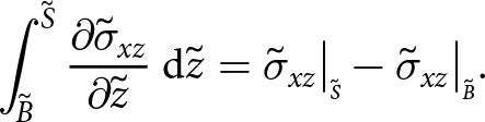
  $\tilde{\sigma}_{xy}$ through the shelf thickness. Depth integration of the $\partial{\tilde{\sigma}_{xz}}/\partial{\tilde{z}}$ term is simpler
 \begin{equation}
\int_{{\tilde{B}}}^{{\tilde{S}}} {{\frac{\partial{\tilde{\sigma}_{xz}}}{\partial{\tilde{z}}}}} \: \mathrm{d}{\tilde{z}} = \tilde{\sigma}_{xz}\big|_{\scriptscriptstyle \tilde{S}} - \tilde{\sigma}_{xz}\big|_{\scriptscriptstyle \tilde{B}}.
\end{equation}
\begin{equation}
\int_{{\tilde{B}}}^{{\tilde{S}}} {{\frac{\partial{\tilde{\sigma}_{xz}}}{\partial{\tilde{z}}}}} \: \mathrm{d}{\tilde{z}} = \tilde{\sigma}_{xz}\big|_{\scriptscriptstyle \tilde{S}} - \tilde{\sigma}_{xz}\big|_{\scriptscriptstyle \tilde{B}}.
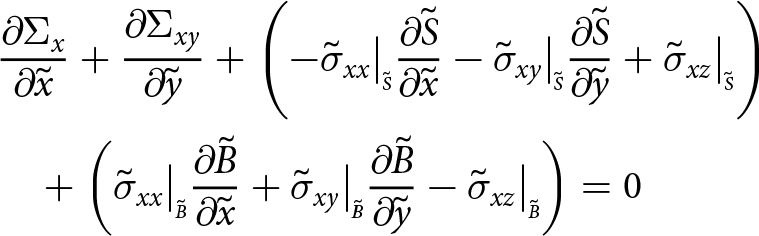
\end{equation}Bringing these integrations together, the first line in Eqn (20) is
 \begin{align}
&{\frac{\partial{\Sigma_{x}}}{\partial{\tilde{x}}}} + {\frac{\partial{\Sigma_{xy}}}{\partial{\tilde{y}}}} + \left( - \tilde{\sigma}_{xx}\big|_{\scriptscriptstyle \tilde{S}}{\frac{\partial{\tilde{S}}}{\partial{\tilde{x}}}} - \tilde{\sigma}_{xy}\big|_{\scriptscriptstyle \tilde{S}}{\frac{\partial{\tilde{S}}}{\partial{\tilde{y}}}} + \tilde{\sigma}_{xz}\big|_{\scriptscriptstyle \tilde{S}} \right) \nonumber\\
&\quad + \left( \tilde{\sigma}_{xx}\big|_{\scriptscriptstyle \tilde{B}}{\frac{\partial{\tilde{B}}}{\partial{\tilde{x}}}} + \tilde{\sigma}_{xy}\big|_{\scriptscriptstyle \tilde{B}}{\frac{\partial{\tilde{B}}}{\partial{\tilde{y}}}} - \tilde{\sigma}_{xz}\big|_{\scriptscriptstyle \tilde{B}} \right) = 0
\end{align}
\begin{align}
&{\frac{\partial{\Sigma_{x}}}{\partial{\tilde{x}}}} + {\frac{\partial{\Sigma_{xy}}}{\partial{\tilde{y}}}} + \left( - \tilde{\sigma}_{xx}\big|_{\scriptscriptstyle \tilde{S}}{\frac{\partial{\tilde{S}}}{\partial{\tilde{x}}}} - \tilde{\sigma}_{xy}\big|_{\scriptscriptstyle \tilde{S}}{\frac{\partial{\tilde{S}}}{\partial{\tilde{y}}}} + \tilde{\sigma}_{xz}\big|_{\scriptscriptstyle \tilde{S}} \right) \nonumber\\
&\quad + \left( \tilde{\sigma}_{xx}\big|_{\scriptscriptstyle \tilde{B}}{\frac{\partial{\tilde{B}}}{\partial{\tilde{x}}}} + \tilde{\sigma}_{xy}\big|_{\scriptscriptstyle \tilde{B}}{\frac{\partial{\tilde{B}}}{\partial{\tilde{y}}}} - \tilde{\sigma}_{xz}\big|_{\scriptscriptstyle \tilde{B}} \right) = 0
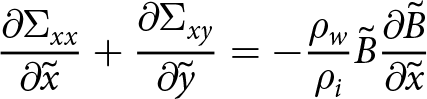
\end{align}and simplifies to, using conditions at the boundaries, and now including the other two dimensions
 \begin{align}
{\frac{\partial{\Sigma_{xx}}}{\partial{\tilde{x}}}} + {\frac{\partial{\Sigma_{xy}}}{\partial{\tilde{y}}}} = - \frac{\rho_w}{\rho_i } \tilde{B} {\frac{\partial{\tilde{B}}}{\partial{\tilde{x}}}}
\end{align}
\begin{align}
{\frac{\partial{\Sigma_{xx}}}{\partial{\tilde{x}}}} + {\frac{\partial{\Sigma_{xy}}}{\partial{\tilde{y}}}} = - \frac{\rho_w}{\rho_i } \tilde{B} {\frac{\partial{\tilde{B}}}{\partial{\tilde{x}}}}
\end{align}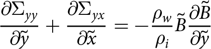 \begin{align}
{\frac{\partial{\Sigma_{yy}}}{\partial{\tilde{y}}}} + {\frac{\partial{\Sigma_{yx}}}{\partial{\tilde{x}}}} = - \frac{\rho_w}{\rho_i } \tilde{B} {\frac{\partial{\tilde{B}}}{\partial{\tilde{y}}}}
\end{align}
\begin{align}
{\frac{\partial{\Sigma_{yy}}}{\partial{\tilde{y}}}} + {\frac{\partial{\Sigma_{yx}}}{\partial{\tilde{x}}}} = - \frac{\rho_w}{\rho_i } \tilde{B} {\frac{\partial{\tilde{B}}}{\partial{\tilde{y}}}}
\end{align}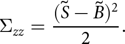 \begin{align}
\Sigma_{zz} = \frac{(\tilde{S} - \tilde{B})^2}{2}.
\end{align}
\begin{align}
\Sigma_{zz} = \frac{(\tilde{S} - \tilde{B})^2}{2}.
\end{align} Equation (25) can be simplified by introducing the shelf thickness,  $\tilde{h}$, which replaces both $\tilde{S} - \tilde{B}$ and $-(\rho_w/\rho_i)\tilde{B}$.
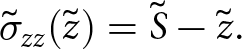
Another vertical integration that will prove to be useful is to integrate Eqn (20c) from an unspecified height,  $\tilde{z}$ to the surface, $\tilde{S}$. This provides the following dimensionless relationship
 \begin{equation}
\tilde{\sigma}_{zz}(\tilde{z}) = \tilde{S} - \tilde{z}.
\end{equation}
\begin{equation}
\tilde{\sigma}_{zz}(\tilde{z}) = \tilde{S} - \tilde{z}.
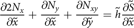
\end{equation}When an incompressible constitutive relationship is used, as is the case for ice flow, the stress tensor components in Eqn (20) can be separated into deviatoric stresses and pressure. A similar vertical integration with appropriate boundary conditions is then used to simplify the equations. This is demonstrated in Appendix 6.3 and results in the familiar SSA,
 \begin{align}
{\frac{\partial{2N_{x}}}{\partial{\tilde{x}}}} + {\frac{\partial{N_{y}}}{\partial{\tilde{x}}}} + {\frac{\partial{N_{xy}}}{\partial{\tilde{y}}}}
= \tilde{h} {\frac{\partial{\tilde{S}}}{\partial{\tilde{x}}}}
\end{align}
\begin{align}
{\frac{\partial{2N_{x}}}{\partial{\tilde{x}}}} + {\frac{\partial{N_{y}}}{\partial{\tilde{x}}}} + {\frac{\partial{N_{xy}}}{\partial{\tilde{y}}}}
= \tilde{h} {\frac{\partial{\tilde{S}}}{\partial{\tilde{x}}}}
\end{align}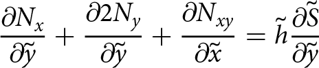 \begin{align}
{\frac{\partial{N_{x}}}{\partial{\tilde{y}}}} + {\frac{\partial{2 N_{y}}}{\partial{\tilde{y}}}} + {\frac{\partial{N_{xy}}}{\partial{\tilde{x}}}}
= \tilde{h} {\frac{\partial{\tilde{S}}}{\partial{\tilde{y}}}}
\end{align}
\begin{align}
{\frac{\partial{N_{x}}}{\partial{\tilde{y}}}} + {\frac{\partial{2 N_{y}}}{\partial{\tilde{y}}}} + {\frac{\partial{N_{xy}}}{\partial{\tilde{x}}}}
= \tilde{h} {\frac{\partial{\tilde{S}}}{\partial{\tilde{y}}}}
\end{align} in which Nx, Ny and Nxy are depth integrations of  $\tilde{\sigma}_{xx}$, $\tilde{\sigma}_{yy}$ and $\tilde{\sigma}_{xy}$ as in Weis Reference Weis(2001). However, incompressibility is not implied by Eqn (25) and the equations are those of a plane problem. This is analogous to plane stress because the field variables are integrated through the depth and the vertical stress $\Sigma_{zz}$ is completely independent of $\Sigma_{xx}$ and $\Sigma_{yy}$ and, therefore, does not contribute to the stress solution in the (x, y) plane. A further simplification to Eqn (25) can be made using the stress tensor decomposition proposed in Lipovsky Reference Lipovsky(2020), demonstrating that the elastic equivalent to the SSA is unequivocally a plane stress problem regardless of whether the elastic constitutive relationship is compressible or not.
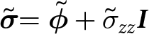
Using the principle of superposition of elastic strain due to different loads, the overburden pressure is subtracted from the total stress tensor. The decomposition is as follows,
 \begin{equation}
\boldsymbol{\tilde{\sigma}} = \boldsymbol{\tilde{\phi}} + \tilde{\sigma}_{zz} \boldsymbol{I}
\end{equation}
\begin{equation}
\boldsymbol{\tilde{\sigma}} = \boldsymbol{\tilde{\phi}} + \tilde{\sigma}_{zz} \boldsymbol{I}
\end{equation} in which  $\boldsymbol{\tilde{\phi}}$ is the stress tensor of interest, is similar to that for deviatoric stresses $\boldsymbol{\tilde{\sigma}}'$. Compression or extension may occur due to sources other than overburden (for example, upstream of an ice rise) and $\boldsymbol{\tilde{\phi}}$ is therefore different from $\boldsymbol{\tilde{\sigma}}'$.
With this decomposition of the Cauchy stress tensor and following the SSA approach, an elastic constitutive relation compatible approximation is achieved. The process is described in detail in Appendix 6.4 and follows these key steps:  $\boldsymbol{\tilde{\sigma}}$ is replaced with $\boldsymbol{\tilde{\phi}}$ and $\tilde{\sigma}_{zz}$ using Eqn (28); $\tilde{\sigma}_{zz}$ is eliminated by substituting the derivative of Eqn (26) in terms of x and y; and then the governing equations are depth-integrated. The first step shows that, to the order of this approximation, the stress $\tilde{\phi}_{zz}$ is zero. The resulting depth-integrated governing equations are those of plane stress,
 \begin{align}
{\frac{\partial{\Phi_{xx}}}{\partial{\tilde{x}}}} + {\frac{\partial{\Phi_{xy}}}{\partial{\tilde{y}}}} = \tilde{h} {\frac{\partial{\tilde{S}}}{\partial{\tilde{x}}}}
\end{align}
\begin{align}
{\frac{\partial{\Phi_{xx}}}{\partial{\tilde{x}}}} + {\frac{\partial{\Phi_{xy}}}{\partial{\tilde{y}}}} = \tilde{h} {\frac{\partial{\tilde{S}}}{\partial{\tilde{x}}}}
\end{align}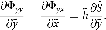 \begin{align}
{\frac{\partial{\Phi_{yy}}}{\partial{\tilde{y}}}} + {\frac{\partial{\Phi_{yx}}}{\partial{\tilde{x}}}} = \tilde{h} {\frac{\partial{\tilde{S}}}{\partial{\tilde{y}}}}.
\end{align}
\begin{align}
{\frac{\partial{\Phi_{yy}}}{\partial{\tilde{y}}}} + {\frac{\partial{\Phi_{yx}}}{\partial{\tilde{x}}}} = \tilde{h} {\frac{\partial{\tilde{S}}}{\partial{\tilde{y}}}}.
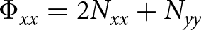
\end{align}The right-hand terms in Eqns (27) and (29) are the same and therefore the left-hand sides of each are equal. This results in the following equivalencies for the depth-integrated stress terms
 \begin{align}
\Phi_{xx} &= 2 N_{xx} + N_{yy}
\end{align}
\begin{align}
\Phi_{xx} &= 2 N_{xx} + N_{yy}
\end{align}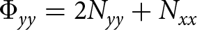 \begin{align}
\Phi_{yy} &= 2 N_{yy} + N_{xx}
\end{align}
\begin{align}
\Phi_{yy} &= 2 N_{yy} + N_{xx}
\end{align} \begin{align}
\Phi_{xy} &= N_{xy}.
\end{align}
\begin{align}
\Phi_{xy} &= N_{xy}.
\end{align}If elastic and viscous stresses are taken to be the same in the deforming ice shelf, then Eqn (30) provides an equivalency for comparing 2D viscous and elastic models. Conceptually, this is a non-linear Maxwell viscoelastic model represented by linear spring in series with a non-linear dashpot in series. In practice, the limited space and time resolution of observational data mean that the above equivalency is likely to only be relevant to infer elastic stresses on viscous timescales.
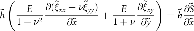
The plane stress approximation in Eqn (29) can be restated in terms of strain and material properties
 \begin{align}
\tilde{h}\left( \frac{E}{1-\nu^2}{\frac{\partial{(\tilde{\xi}_{xx} + \nu\tilde{\xi}_{yy})}}{\partial{\tilde{x}}}} + \frac{E}{1+\nu}{\frac{\partial{\tilde{\xi}_{xy}}}{\partial{\tilde{y}}}} \right) = \tilde{h}{\frac{\partial{\tilde{S}}}{\partial{\tilde{x}}}}
\end{align}
\begin{align}
\tilde{h}\left( \frac{E}{1-\nu^2}{\frac{\partial{(\tilde{\xi}_{xx} + \nu\tilde{\xi}_{yy})}}{\partial{\tilde{x}}}} + \frac{E}{1+\nu}{\frac{\partial{\tilde{\xi}_{xy}}}{\partial{\tilde{y}}}} \right) = \tilde{h}{\frac{\partial{\tilde{S}}}{\partial{\tilde{x}}}}
\end{align} \begin{align}
\tilde{h}\left( \frac{E}{1-\nu^2}{\frac{\partial{(\tilde{\xi}_{yy} + \nu\tilde{\xi}_{xx})}}{\partial{\tilde{y}}}} + \frac{E}{1+\nu}{\frac{\partial{\tilde{\xi}_{xy}}}{\partial{\tilde{x}}}} \right) = \tilde{h}{\frac{\partial{\tilde{S}}}{\partial{\tilde{y}}}}
\end{align}
\begin{align}
\tilde{h}\left( \frac{E}{1-\nu^2}{\frac{\partial{(\tilde{\xi}_{yy} + \nu\tilde{\xi}_{xx})}}{\partial{\tilde{y}}}} + \frac{E}{1+\nu}{\frac{\partial{\tilde{\xi}_{xy}}}{\partial{\tilde{x}}}} \right) = \tilde{h}{\frac{\partial{\tilde{S}}}{\partial{\tilde{y}}}}
\end{align} in which  $\boldsymbol{\tilde{\xi}}$ is the strain associated with $\boldsymbol{\tilde{\phi}}$ and the material properties are assumed constant with depth. Alternatively, depth-integrated strain and material properties can be used.
The condition at the front in Eqn (B3) must also be vertically integrated in order to complete a 2D model of the shelf,
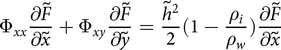 \begin{align}
\Phi_{xx}{\frac{\partial{\tilde{F}}}{\partial{\tilde{x}}}} + \Phi_{xy}{\frac{\partial{\tilde{F}}}{\partial{\tilde{y}}}} = \frac{\tilde{h}^2}{2}(1-\frac{\rho_i}{\rho_w}){\frac{\partial{\tilde{F}}}{\partial{\tilde{x}}}}
\end{align}
\begin{align}
\Phi_{xx}{\frac{\partial{\tilde{F}}}{\partial{\tilde{x}}}} + \Phi_{xy}{\frac{\partial{\tilde{F}}}{\partial{\tilde{y}}}} = \frac{\tilde{h}^2}{2}(1-\frac{\rho_i}{\rho_w}){\frac{\partial{\tilde{F}}}{\partial{\tilde{x}}}}
\end{align}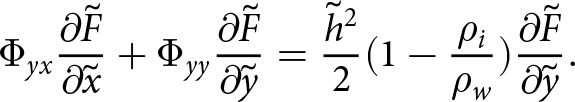 \begin{align}
\Phi_{yx}{\frac{\partial{\tilde{F}}}{\partial{\tilde{x}}}} +\Phi_{yy}{\frac{\partial{\tilde{F}}}{\partial{\tilde{y}}}} = \frac{\tilde{h}^2}{2}(1-\frac{\rho_i}{\rho_w}){\frac{\partial{\tilde{F}}}{\partial{\tilde{y}}}}.
\end{align}
\begin{align}
\Phi_{yx}{\frac{\partial{\tilde{F}}}{\partial{\tilde{x}}}} +\Phi_{yy}{\frac{\partial{\tilde{F}}}{\partial{\tilde{y}}}} = \frac{\tilde{h}^2}{2}(1-\frac{\rho_i}{\rho_w}){\frac{\partial{\tilde{F}}}{\partial{\tilde{y}}}}.
\end{align}It is thus shown that the ice shelf can be represented elastically as a 2D plane stress problem for all strains that are not due to glaciostatic overburden pressure. If required, the full strain or stress field can be obtained from the displacement solution for the glaciostatic stress, given here in dimensional form:
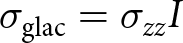 \begin{align}
\sigma_{\text{glac}} &= \sigma_{zz} I
\end{align}
\begin{align}
\sigma_{\text{glac}} &= \sigma_{zz} I
\end{align}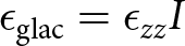 \begin{align}
\epsilon_{\text{glac}} &= \epsilon_{zz} I
\end{align}
\begin{align}
\epsilon_{\text{glac}} &= \epsilon_{zz} I
\end{align} \begin{align}
\epsilon_{zz} &= \frac{E}{(1-2\nu)}(S-z)g\rho_i.
\end{align}
\begin{align}
\epsilon_{zz} &= \frac{E}{(1-2\nu)}(S-z)g\rho_i.
\end{align}3. 2D solutions to a 3D rift problem
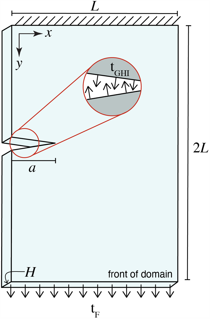
The preceding derivation establishes the elastic plane problem and the appropriate comparison between elastic plane stresses and viscous deviatoric stresses should they be conceptually linked, as for example, with an assumption of non-linear Maxwell viscoelasticity. While representative of the problem at ice-shelf scale, both approximations are limited near boundaries where the underlying assumptions may not be satisfied (Weis, Reference Weis2001). This is particularly relevant at floating boundaries, where a depth-dependent load results from the glaciostatic and hydrostatic imbalance (GHI) acting on the ice face (Fig. 4). Next, 2D and 3D representations of a rift front are compared in order to understand the limitations of the plane view with regard to the inherently 3D GHI (Figs 2 and 3).
The models presented in this section are representative of a subsection of shelf in close proximity to the tip (2D) or front (3D).
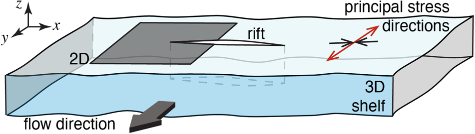
The propagating end of a rift is a line for a 3D representation and a point for a 2D representation. The GHI acts on all shelf surfaces including rift walls and is plotted in Figure 4.

Rift walls are subject to the same conditions as at the shelf front, provided that both are assumed to be in contact with ocean water and atmosphere only. When using the tensor  $\boldsymbol{\tilde{\phi}}$, as is the case here, the glacial overburden pressure is removed from the problem setup. At the front of the shelf, this results in the boundary condition being precisely the GHI. In the case of a 2D problem the depth integration of the boundary condition is described in Eqn (32). The associated traction $\boldsymbol{t_{GHI}}$ is normal to the surface and takes on the form
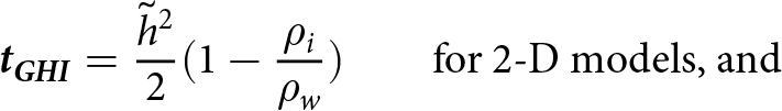 \begin{align}
\boldsymbol{t_{GHI}} = \frac{\tilde{h}^2}{2}(1-\frac{\rho_i}{\rho_w}) \quad \quad \text{for\ 2D\ models,\ and}
\end{align}
\begin{align}
\boldsymbol{t_{GHI}} = \frac{\tilde{h}^2}{2}(1-\frac{\rho_i}{\rho_w}) \quad \quad \text{for\ 2D\ models,\ and}
\end{align} \begin{align}
\boldsymbol{t_{GHI}}(\tilde{z}) = \begin{cases}
\tilde{S} - \tilde{z} & \quad \tilde{z} \gt 0 \\
\tilde{S}-\tilde{z} ( 1 - \frac{\rho_{w}}{\rho_i} ) & \quad \tilde{z} \lt 0 \end{cases} \quad \quad \text{for\ 3D\ models}.
\end{align}
\begin{align}
\boldsymbol{t_{GHI}}(\tilde{z}) = \begin{cases}
\tilde{S} - \tilde{z} & \quad \tilde{z} \gt 0 \\
\tilde{S}-\tilde{z} ( 1 - \frac{\rho_{w}}{\rho_i} ) & \quad \tilde{z} \lt 0 \end{cases} \quad \quad \text{for\ 3D\ models}.
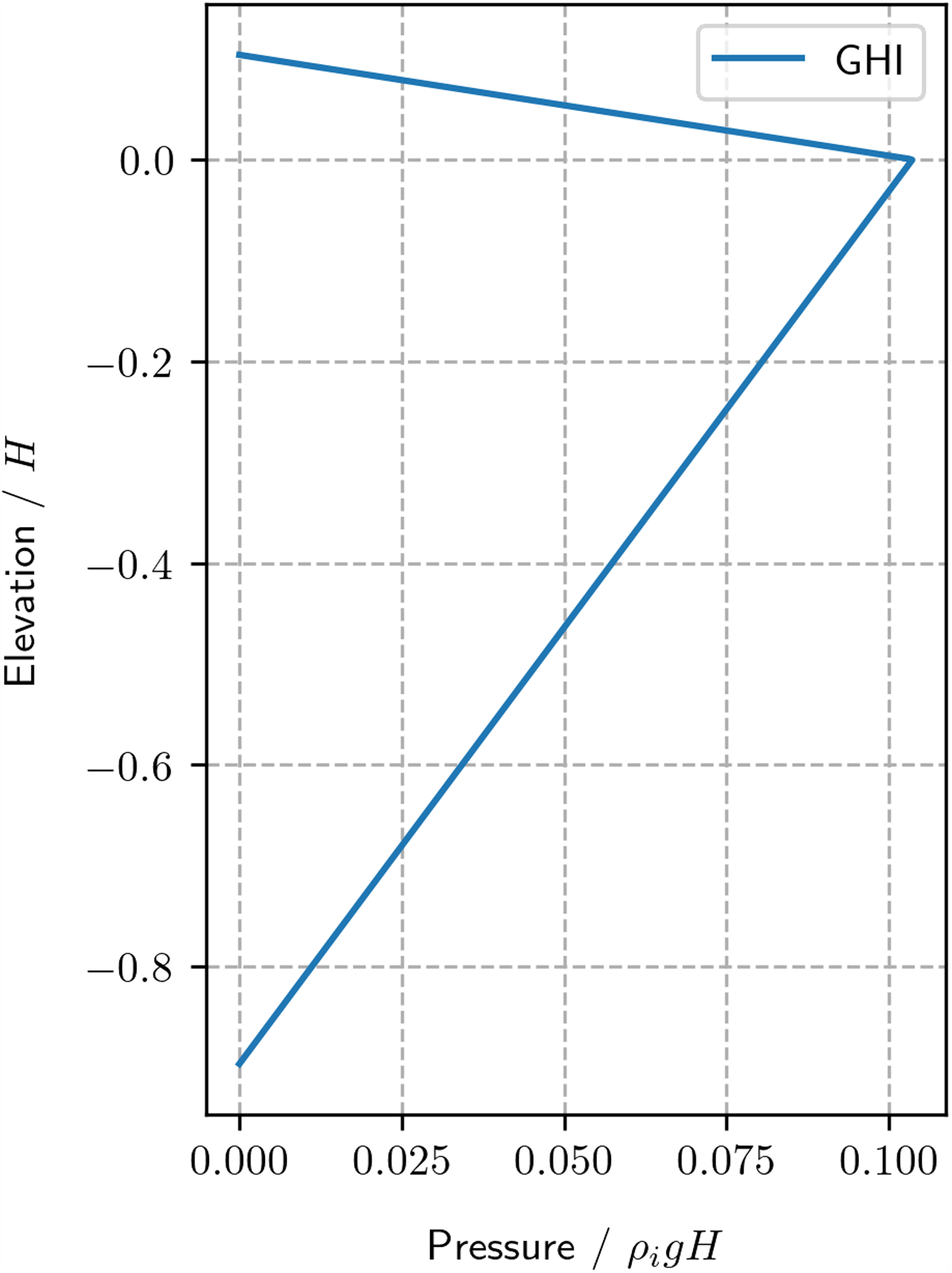
\end{align}The GHI is plotted for a non-dimensional shelf face in Fig. 4.
The non-dimensional glaciostatic and hydrostatic overburden imbalance (GHI) on a shelf face (front or rift). The vertical coordinate is the non-dimensional thickness. Positive is here taken to be outward from the ice (pulling on the face). With constant ice and seawater densities of 917 kg m−3 and 1023 kg m−3, the ice cliff height is 0.104.
A 3D analytical solution from (Tada and others, Reference Tada, Paris and Irwin1985) can be used to develop intuition about the effect of the rift-wall loading on SIFs at a rift front. The most appropriate analytical solution available is for point loads on crack walls in an infinite, rather than finite, thickness layer. In Appendix 6.5, these point loads are scaled and integrated to simulate the GHI and explore the effects on SIFs at rift fronts in an infinite medium.
3.1. Comparing SIFs from 3D and plane stress models
A link is established between the 3D and 2D views by comparing SIFs from idealised models designed to isolate the effects of the GHI on SIFs. In both cases, SIFs are calculated using the displacement correlation method (DCM; Gupta and others, Reference Gupta, Duarte and Dhankhar2017, Jiménez and Duddu, Reference Jiménez and Duddu2018, Lipovsky, Reference Lipovsky2020). The DCM is an analytical technique in LEFM that can be used to approximately determine SIFs by correlating the displacements measured near the crack tip with the appropriate (plane stress or plane strain) theoretical displacements. The following displacement solutions from Gupta and others Reference Gupta, Duarte and Dhankhar(2017) are used here:
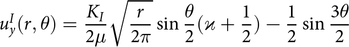 \begin{align}
u_{y}^{I}(r,\theta) &= \frac{K_{I}}{2\mu}\sqrt{\frac{r}{2\pi}}\sin{\frac{\theta}{2}}(\varkappa + \frac{1}{2} )-\frac{1}{2}\sin{\frac{3\theta}{2}}
\end{align}
\begin{align}
u_{y}^{I}(r,\theta) &= \frac{K_{I}}{2\mu}\sqrt{\frac{r}{2\pi}}\sin{\frac{\theta}{2}}(\varkappa + \frac{1}{2} )-\frac{1}{2}\sin{\frac{3\theta}{2}}
\end{align}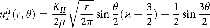 \begin{align}
u_{x}^{II}(r,\theta) &= \frac{K_{II}}{2\mu}\sqrt{\frac{r}{2\pi}}\sin{\frac{\theta}{2}}(\varkappa - \frac{3}{2})+\frac{1}{2}\sin{\frac{3\theta}{2}}
\end{align}
\begin{align}
u_{x}^{II}(r,\theta) &= \frac{K_{II}}{2\mu}\sqrt{\frac{r}{2\pi}}\sin{\frac{\theta}{2}}(\varkappa - \frac{3}{2})+\frac{1}{2}\sin{\frac{3\theta}{2}}
\end{align}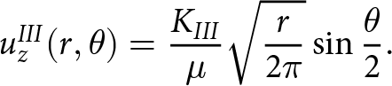 \begin{align}
u_{z}^{III}(r,\theta) &= \frac{K_{III}}{\mu} \sqrt{\frac{r}{2\pi}}\sin{\frac{\theta}{2}}.
\end{align}
\begin{align}
u_{z}^{III}(r,\theta) &= \frac{K_{III}}{\mu} \sqrt{\frac{r}{2\pi}}\sin{\frac{\theta}{2}}.
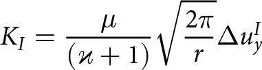
\end{align} The SIFs are calculated using measured displacements between the two walls  $\Delta u_x$ and $\Delta u_y$, using the following expressions derived from Eqn (35):
 \begin{align}
K_{I} &= \frac{\mu}{(\varkappa+1)}\sqrt{\frac{2 \pi}{r}}\Delta{u_{y}^I}
\end{align}
\begin{align}
K_{I} &= \frac{\mu}{(\varkappa+1)}\sqrt{\frac{2 \pi}{r}}\Delta{u_{y}^I}
\end{align} \begin{align}
K_{II} &= \frac{\mu}{(\varkappa+1)}\sqrt{\frac{2 \pi}{r}}\Delta{u_{x}^{II}}
\end{align}
\begin{align}
K_{II} &= \frac{\mu}{(\varkappa+1)}\sqrt{\frac{2 \pi}{r}}\Delta{u_{x}^{II}}
\end{align}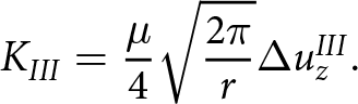 \begin{align}
K_{III} &= \frac{\mu}{4}\sqrt{\frac{2 \pi}{r}}\Delta{u_{z}^{III}}.
\end{align}
\begin{align}
K_{III} &= \frac{\mu}{4}\sqrt{\frac{2 \pi}{r}}\Delta{u_{z}^{III}}.
\end{align} The constant (Kolosov)  $\varkappa$ is
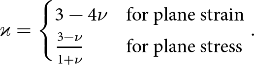 \begin{equation}
\varkappa =
\begin{cases}
3 - 4\nu & \text{for\ plane\ strain} \\
\frac{3-\nu}{1+\nu} & \text{for\ plane\ stress}
\end{cases}.
\end{equation}
\begin{equation}
\varkappa =
\begin{cases}
3 - 4\nu & \text{for\ plane\ strain} \\
\frac{3-\nu}{1+\nu} & \text{for\ plane\ stress}
\end{cases}.
\end{equation} In practice, sets of radially emanating pairs of points on opposite sides of the crack are used to reduce the mismatch of the fit to the ideal solutions (Jiménez and Duddu, Reference Jiménez and Duddu2018). In the present work, an averaging scheme proposed in Gupta and others Reference Gupta, Duarte and Dhankhar(2017) is used for ten pairs of points within  $H/5$ of the rift front or tip. The DCM is applied using the plane strain coefficient in Eqn (37) at different depths within the 3D model to obtain SIFs as a function of depth. In the 2D model, the DCM is applied with a plane stress coefficient (Tada and others, Reference Tada, Paris and Irwin1985).
3.2. Model implementation
The 3D model domain is a  $2L \times L \times H$ shelf section with homogeneous mechanical properties and a through-cutting rift (Fig. 6). The rift is explicitly represented as a sharp wedge, $0.0002*H$ in width at the domain edge, of length a and perpendicular to the edge it bisects (Fig. 5). All dimensions in the model are scaled to the constant thickness H and some care is required in interpreting figures of results in this section as factors of varying powers of H are therefore involved.
The 3D model domain and dimensions. A comparison is made to an equivalent 2D domain, the surface plane, using plane stress. In the 3D model domain, the rift wall traction,  $\boldsymbol{t_{GHI}}$, is the GHI and depends on the depth and the traction at the front of the domain, $\boldsymbol{t_F}$, is constant with depth and has components $(t_x,t_y)$. For the 2D plane stress model, the rift wall traction and the traction at the front are the same.
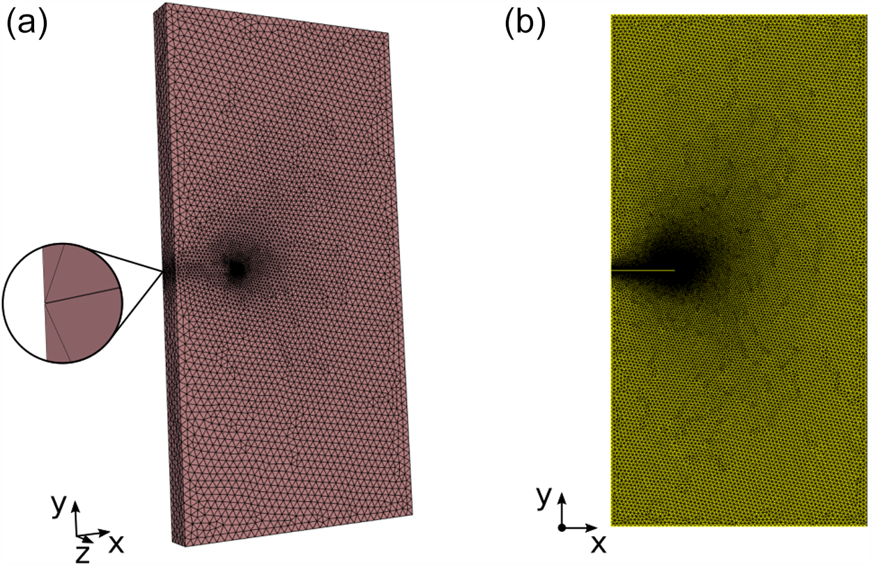
Examples of (a) 3D and (b) 2D meshes generated with Gmsh for FEniCS simulations of stresses at the rift tip. The 3D mesh includes an enlargement of the gap between the rift walls on the leftmost side.
Boundary conditions on the 3D domain are chosen to represent a small rift in an approximately uniform stress field (Fig. 2). One end of the domain is held fixed in all directions and the opposite end is loaded with a depth-constant traction. This boundary condition is used to simulate loading from surrounding ice shelf rather than simulate a small shelf with a centre rift. All vertical faces except for the one bisected by the rift are fixed in the  $\vec{\boldsymbol{z}}$ direction. The face bisected by the rift is fixed in the direction of the rift, the $\vec{\boldsymbol{x}}$ direction, to enact a symmetry condition that makes this domain comparable to a square ( $2L \times 2L$) testcase with a horizontal centre crack. The front of the domain is loaded with a constant traction, $\boldsymbol{t_F}$, which has components $(t_x,t_y)$. The components $(t_x,t_y)$ are scaled to be either multiples or fractions of the depth-averaged GHI tG. Empirically validated analytical formulations, in this case 2.34 is used, for the SIFs of centre crack cases are provided in Tada and others Reference Tada, Paris and Irwin(1985). All domains in this section are created and meshed with Gmsh (Geuzaine and Remacle, Reference Geuzaine and Remacle2009). Surfaces are meshed using triangular elements and volumes are meshed using tetrahedral elements.
The domain is used with the governing equations written in terms of ϕ. This is advantageous because the model mesh is made representative of ice after glaciostatic compression, avoiding deformation of the mesh by the overburden pressure (which is not of interest). The elastostatic BVP problem is solved using FEniCS, an opensource library for writing models in their variational form (A. Logg, Reference Logg, Mardal and Wells2012, Alnaes and others, Reference Alnaes2015).
3.3. Mesh and configuration sensitivity
Mesh resolution may affect the accuracy of the numerical result and domain configuration may introduce boundary effects where a rift front becomes close to a domain boundary. These issues are examined in a sensitivity study using a test domain with  $L = 8H$ and depth-constant traction $\boldsymbol{t_F}$, equivalent to the average traction due to the GHI, normal to the front surface, imposed on the rift front. The initial rift length is $a = 2H$. The mesh is designed to be scaled with respect to three different regions of the model domain: the rift front, the rift walls and the rest of the domain.
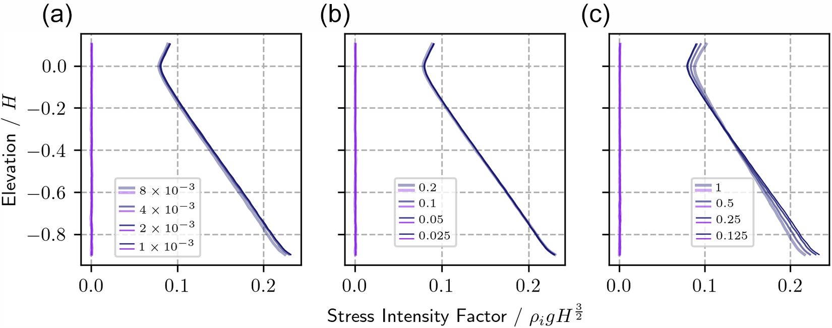
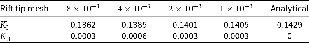
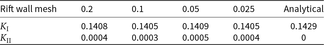
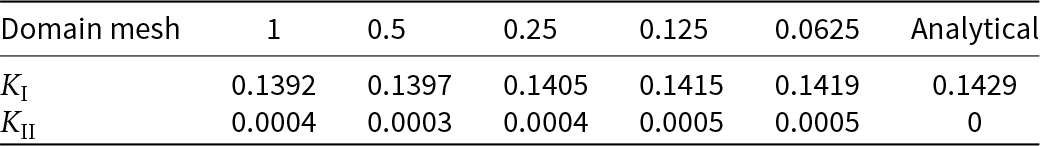
Suitable mesh resolution is identified qualitatively, using the patterns of SIFs obtained at the rift front (Fig. 7). Within the range of element sizes explored, the rift front SIFs are found to be most sensitive to mesh element size within the domain (Fig. 7c). Henceforth, meshes are made using a rift tip mesh size of  $ (4\times10^{-3})H$, rift wall element size of 0.1H and domain element size of 0.25H. An analysis of the importance of rift tip, rift wall and domain element sizes for 2D models is compiled in Tables 2–4. Henceforth, 2D meshes are made using $H \times 10^{-3}$ for the rift-tip mesh size, 0.025H for the rift-wall mesh size and 0.125H for the rift-domain mesh size.
Depth profiles of  $K_\mathrm{I}$ in dark blue and $K_\mathrm{II}$ in purple for varying mesh sizes at (a) the rift tips, (b) walls and (c) in the remaining domain. The mesh size dimensions in each legend are factors of H. For example, $8 \times 10^{-3}$ in panel (a) means the rift tip elements are $H*8\times 10^{-3}$. For this sensitivity analysis, the rift length is $a=2H$ and the domain width is $L=8H$. The traction $\boldsymbol{t_F}$ at the front of the domain has only a component normal to the front, ty, which is equal to the depth averaged GHI traction tG.
Sensitivity of the 2D domain to rift-tip element size. Mesh sizes are given as factors of H
Sensitivity of the 2D domain to rift-wall element size
Sensitivity of the 2D domain to rift-domain element size
The general testcase geometry is also evaluated. SIF profile shapes may depend on the relationship between rift length and domain size because this affects rift proximity to domain boundaries. For ease of comparison, the traction applied to the front of the domain is scaled to obtain constant 2D SIF magnitudes. This causes the 3D profiles to overlay each other and facilitates their comparison. The SIF profile is found to be insensitive to the domain size provided the rift length does not bisect too much of the domain (Fig. 8a). This shows that the testcase adequately isolates the rift from domain boundary effects (other than the GHI acting on the rift walls). $K_\mathrm{I}$ and $K_\mathrm{II}$ profiles for varying domain and rift sizes. (a) Model domain length, b, is varied from 4H to 32H and rift length is maintained at 2H. (b) Rift length is increased from 2H to 12H and the domain is maintained at 32H. The rift length in panel (b) is maintained below a 2:5 ratio of the domain length as this is the rift length to domain length ratio past which $K_\mathrm{I}$ profiles change appreciably in panel (a).
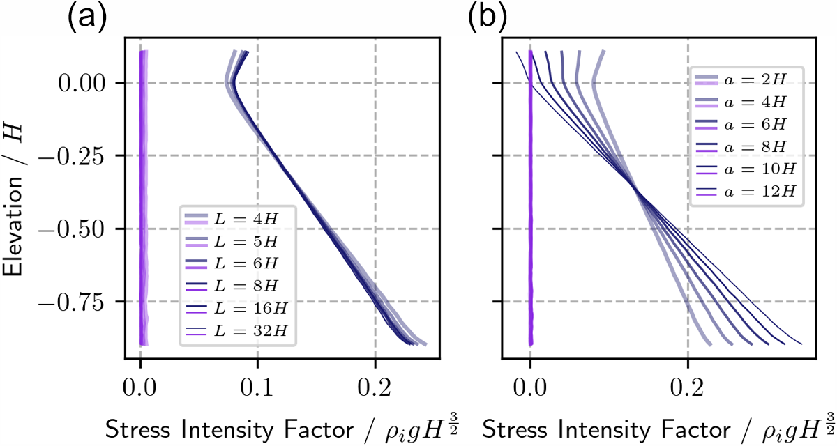
Rift length affects vertical variation in the SIFs (Fig. 8b). Would the GHI not be applied to the rift walls, we could expect SIFs to increase as a function of the square root of the length of the rift. This contribution is in competition with the length of GHI contributing to keeping the rift closed. Longer lengths of GHI loading on rift walls leads to steeper profiles of SIFs at the rift front, meaning a greater tendency for rifts to propagate at depth and remain closed at the top surface.
3.4. 3D and 2D comparison
Results generated using the 3D model with optimum mesh sizes and a rift length of  $a = 2H$ are now compared to their 2D plane stress counterparts. The size of the domain is always maintained such that
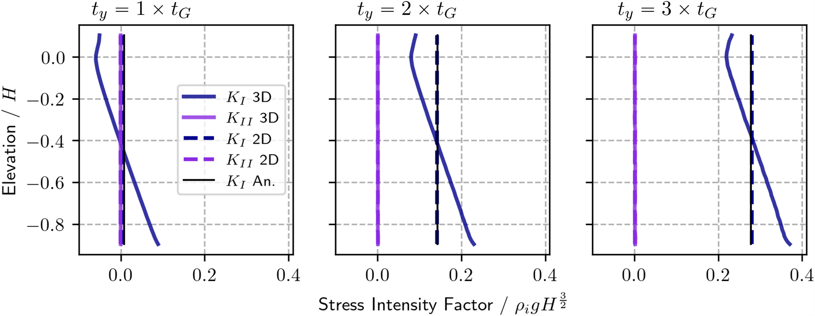
  $L=8H$. 3D SIF profiles are shown to be well-approximated by the 2D models. In Fig. 9, the tractions at the front of the domain are normal and increase in multiples of the depth-averaged GHI. The first panel in Fig. 9 is recreated in Appendix 6.6 using a 300 m thick ice shelf as a demonstration of the range of SIF values that these non-dimensional results represent. In Fig. 10, the traction at the front is applied in the direction of the rift, $\vec{\boldsymbol{x}}$, increasing by fractions of the depth-averaged GHI. In this manner, significant shearing also occurs and $K_\mathrm{II}$ may also be investigated. In Fig. 11, the traction acting on the rift walls is removed. $K_\mathrm{III}$ is also investigated for the 3D models and can be found in Appendix 6.7.
Depth profiles and 2D results for  $K_\mathrm{I}$ and $K_\mathrm{II}$ at the front/tip of a rift in a symmetrical $8H \times 16H \times H$ section of shelf. The rift walls are loaded with the GHI, $\boldsymbol{t_{GHI}}$. The traction at the front, $\boldsymbol{t_F}$ has only a component normal to the front, ty, which is equal to $Y \times t_G$, where $Y = 1,2,3$ for plots from left to right.
Depth profiles and 2D results for  $K_\mathrm{I}$ and $K_\mathrm{II}$ at the front/tip of a rift in a symmetrical $8H \times 16H \times H$ section of shelf. The rift walls are loaded with the GHI, $\boldsymbol{t_{GHI}}$. The traction at the front, $\boldsymbol{t_F}$, has only the component tangential to the model front, tx, which is $X \times t_G$, where $X = 0.2,0.4,0.6$ for plots from left to right.

Depth profiles and 2D results for  $K_\mathrm{I}$ and $K_\mathrm{II}$ at the front/tip of a rift in a symmetrical $8H \times 16H \times H$ section of shelf. The rift walls are not loaded with the GHI. The traction at the front, $\boldsymbol{t_F}$ has only a component normal to the front, ty, which is equal to $Y \times t_G$, where $Y = 1,2,3$ for plots from left to right.

4. Discussion
Fractures propagate in response to a stress field in the ice, resolved at the location of propagation. By breaking and creating new boundaries in the material, fractures modify that field. Simulation of crevasse and rift behaviour, then, requires the stress field to be known and to be updated as propagation occurs. Both theoretical and applied challenges arise from the requirement to update the stress field during propagation. A fully viscoelastic constitutive relationship would allow for a direct theoretical update of the stress field though in that case, propagation rate must be resolved and for 2D models, the two approximations somehow simultaneously satisfied. The present contribution is grounded in the theoretical worldview of the SSA, enabling stresses from a 2D viscous simulation to be linked with an equivalent elastic problem. Decomposing the problem into viscous and elastic components (van der Veen, Reference van der Veen1998, Hulbe and others, Reference Hulbe, LeDoux and Cruikshank2010, Plate and others, Reference Plate, Gross, Humbert and Müller2012) is akin to applying a non-linear Maxwell viscoelasticity. A similar conceptual framework is employed to link viscous and elastic stress fields for rapidly evolving damage in Huth and others Reference Huth, Duddu, Smith and Sergienko(2023). It is important to note that the reverse approach—taking the stress field from an elastic model and imposing it on a viscous flow model—is not likely relevant, as even small strains will modify boundary conditions around the rift and invalidate elastic solutions on viscous timescales.
A proposed approach to a stepped viscous and elastic model of ice-shelf rifts using the SSA and plane stress is as follows. A viscous SSA solution that matches a derived velocity field for an interval in which the studied rift is not observed to be propagating is used to obtain an initial stress field to be applied to the elastic problem. Assuming propagation rates to be fast enough that viscous deformation is insignificant, the plane stress elastic problem is then used to simulate propagation with standard fracture mechanics approaches, in which the elastic stress field updates as the rift geometry changes. Propagation should continue until complete separation of the shelf or stress conditions warrant arrest (i.e. SIFs fall bellow fracture toughness values for ice). The effect of rift front geometry and depth-dependence of SIFs on propagation and arrest conditions should be considered. If the effect of rift propagation on the shelf flow is the object of the study, the viscous flow model would then be modified to reflect the presence of the lengthened rift via new boundary conditions or updates to spatially varying rheological parameters that represent the presence of rifts.
In most applied studies, stresses are inferred from observations of viscous deformation using the SSA. These inversions provide good insight into the stress state while managing spatial heterogeneity by adjusting the stiffness parameter in the flow law (MacAyeal, Reference MacAyeal1993, Rommelaere and MacAyeal, Reference Rommelaere and MacAyeal1997, Vieli and Payne, Reference Vieli and Payne2003, Goldberg and Sergienko, Reference Goldberg and Sergienko2011). However, the time resolution of observational data may not be matched with rift propagation. By creating internal boundaries, rifts locally modify the deformation field on timescales that are poorly resolved and unrelated to the stiffness parameter.
In numerical 3D crack problems, SIFs are calculated at points along the front in a local coordinate systems defined by the front’s geometry, with one crack-front-tangent component and two components in the front-perpendicular plane (for example,
Shih and others, Reference Shih, Moran and Nakamura1986, Sukumar and others, Reference Sukumar, Moës, Moran and Belytschko2000, Gosz and Moran, Reference Gosz and Moran2002, Daimon and Okada, Reference Daimon and Okada2014).  $K_\mathrm{I}$ and $K_\mathrm{II}$ depend on plane strain field values, strain or stress, in the front-perpendicular plane only (Gosz and Moran, Reference Gosz and Moran2002). If a 3D rift front is assumed to be vertical (the rift-front and gravity are aligned), then the overburden pressure is constant throughout the front-perpendicular plane at the fracture mechanics relevant scales and does not contribute to SIFs. Consequently, only ϕ, the stress tensor with that pressure removed, is required to obtain SIFs relevant for horizontal propagation of rifts. This is the case for other elastic ice-shelf applications because compression from overburden is rarely relevant (for example,
Still and others, Reference Still2022). However, the overburden pressure may be relevant to material properties that affect propagation (Liu and Ravichandran, Reference Liu and Ravichandran2006) and it can be easily reintroduced to the solution stress or strain field using Eqn (33).
$K_\mathrm{II}$ depend on plane strain field values, strain or stress, in the front-perpendicular plane only (Gosz and Moran, Reference Gosz and Moran2002). If a 3D rift front is assumed to be vertical (the rift-front and gravity are aligned), then the overburden pressure is constant throughout the front-perpendicular plane at the fracture mechanics relevant scales and does not contribute to SIFs. Consequently, only ϕ, the stress tensor with that pressure removed, is required to obtain SIFs relevant for horizontal propagation of rifts. This is the case for other elastic ice-shelf applications because compression from overburden is rarely relevant (for example,
Still and others, Reference Still2022). However, the overburden pressure may be relevant to material properties that affect propagation (Liu and Ravichandran, Reference Liu and Ravichandran2006) and it can be easily reintroduced to the solution stress or strain field using Eqn (33).
Interpreting stresses from a viscous plane problem for fracture requires caution. Assuming that elastic stresses are the same as viscous stresses, the elastic stress tensor that is relevant for brittle fracture is the composition of depth-integrated deviatoric stress components as described in Eqn (30). That is the total (Cauchy) stress tensor with the overburden subtracted from it and in the 2D case, depth-integrated. 2D approaches that interpret stress or strain to update either explicit or diffuse fractures should use this plane stress tensor. In the 3D case, the same tensor is required without depth integration. Although including the overburden pressure is also correct it does not directly contribute to SIFs of a horizontally propagating rift. The integrated GHI on the rift walls is the only means by which the weight of ice and water-pressure impact these SIFs.
Decomposition of the stress tensor resulting in ϕ also provides a straightforward way to consider the effect of ocean water filling through-cutting rifts. When ϕ is used, the boundary condition on a rift becomes the imbalance between glaciostatic and hydrostatic overburdens (GHI). If no other material is present within a rift, an extensional stress sufficient to overcome the inward pull of the GHI is required for separation of the rift walls. This provides a simple limit on the formation of rifts. Extensional stresses within the shelf must be larger than the (thickness-dependent) GHI within the rift.
The GHI contributes to depth-dependence in mode I SIFs at the rift front. From the sea surface to the base of the ice shelf, mode I SIFs increase. Above the sea surface, the depth dependence varies with rift length. The present work focuses on SIFs below the sea surface. In other works, the effect of the GHI is described as a bending moment on the rift walls (Lipovsky, Reference Lipovsky2020). The greater the rift length, the greater the magnitude of the depth-dependence. This suggests that in the absence of other effects, the lateral extent of rifts should be greater at the lower ice-shelf surface than at the upper surface and the longer the rift, the greater this mismatch should be. However, other contributions to the stress balance on rift walls are likely, for example, partial contact between walls (Lipovsky, Reference Lipovsky2020) and mélange acting on the rift walls (Bassis and others, Reference Bassis2007, Huth and others, Reference Huth, Duddu, Smith and Sergienko2023). These contributions are also likely to depend on rift length and the distance between rift walls. Further work is required to explore how non-vertical fronts alleviate mismatches in mode one SIFs at the front.
In our 3D models, negative values are obtained for  $K_\mathrm{I}$ at particular depths for certain loading conditions. While it is safe to say these are depths at which propagation will not be favoured under those conditions, the negative values do imply rift-inward displacements on the rift walls, which may lead to non-physical interpenetration. Managing interpenetration via numerical contact techniques would alter the SIFs in these locations and the net contribution would be larger depth-averaged $K_\mathrm{I}$ along the rift front.
5. Conclusion
Rift and crevasse propagation in glacier ice is an inherently 3D problem for which 2D simplifications are highly desirable and useful. This simplification can be made in either the vertical (rifts) or horizontal (crevasses) direction and various cases have been studied in this way. For example, stresses derived from observed viscous deformation are widely used to study rift propagation and tabular iceberg calving. Such studies include validation by comparison of model outputs with what can be observed directly, such as surface traces of rifts. Here, we examine the relationship between the 3D and 2D problems for this case and in so doing, provide theoretical verification for practical applications requiring a 2D approach. This also provides a theoretical link with the 3D-to-2D simplifications widely used in computational simulation of ice flow.
The present work demonstrates that plane stress should be used when simulating horizontal strain for an elastic ice shelf even though the fracture mechanics conditions at a given depth along a rift tip are those of plane strain. The comparison also leads to new insight into the geometry of the rift tip. Depth-dependence of the GHI results in depth dependence in  $K_\mathrm{I}$ SIFs (Figs 9–10) (as in
Lipovsky, Reference Lipovsky2020). The magnitude of that dependence increases with rift length contrary to what was noted the analytical solutions in Fig. 12. The depth-dependence implies that rift length should be greater at depth than at sea level, such that rift fronts should tend not to be vertical.
$K_\mathrm{I}$ SIFs (Figs 9–10) (as in
Lipovsky, Reference Lipovsky2020). The magnitude of that dependence increases with rift length contrary to what was noted the analytical solutions in Fig. 12. The depth-dependence implies that rift length should be greater at depth than at sea level, such that rift fronts should tend not to be vertical.  $K_\mathrm{II}$ and $K_\mathrm{III}$ exhibit very small depth-dependence which we attribute to a perturbation due to the intersection of rift front with the upper or lower surface of the ice shelf (Bazant and Estenssoro, Reference Bazant and Estenssoro1979).
Data availability statement
Numerical models used in this work are freely available on github at https://github.com/mforb/2Dv3D_rift_FEniCS.git.
Acknowledgements
The authors are grateful to the scientific editor (Thanks Ralf) and two anonymous reviewers for their time and thoughtfulness in helping to improve the clarity of the manuscript. This work was supported by the Aotearoa New Zealand Antarctic Science Platform (ANTA1801) Antarctic Ice Dynamics Project (ASP02101) and a University of Otago Division of Sciences strategic scholarship to Martin Forbes.
Appendix A
The dimensionless boundary conditions at the surface, base and front of the shelf are provided here.  $S(x,y)$ and $B(x,y)$ are functions for elevation and must be scaled as such. The surface condition becomes
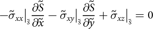 \begin{align}
-\tilde{\sigma}_{xx}\big|_{\scriptscriptstyle \tilde{S}}{\frac{\partial{\tilde{S}}}{\partial{\tilde{x}}}} -\tilde{\sigma}_{xy}\big|_{\scriptscriptstyle \tilde{S}}{\frac{\partial{\tilde{S}}}{\partial{\tilde{y}}}}+ \tilde{\sigma}_{xz}\big|_{\scriptscriptstyle \tilde{S}} &= 0
\end{align}
\begin{align}
-\tilde{\sigma}_{xx}\big|_{\scriptscriptstyle \tilde{S}}{\frac{\partial{\tilde{S}}}{\partial{\tilde{x}}}} -\tilde{\sigma}_{xy}\big|_{\scriptscriptstyle \tilde{S}}{\frac{\partial{\tilde{S}}}{\partial{\tilde{y}}}}+ \tilde{\sigma}_{xz}\big|_{\scriptscriptstyle \tilde{S}} &= 0
\end{align} \begin{align}
-\tilde{\sigma}_{yx}\big|_{\scriptscriptstyle \tilde{S}}{\frac{\partial{\tilde{S}}}{\partial{\tilde{x}}}} -\tilde{\sigma}_{yy}\big|_{\scriptscriptstyle \tilde{S}}{\frac{\partial{\tilde{S}}}{\partial{\tilde{y}}}}+ \tilde{\sigma}_{yz}\big|_{\scriptscriptstyle \tilde{S}} &= 0
\end{align}
\begin{align}
-\tilde{\sigma}_{yx}\big|_{\scriptscriptstyle \tilde{S}}{\frac{\partial{\tilde{S}}}{\partial{\tilde{x}}}} -\tilde{\sigma}_{yy}\big|_{\scriptscriptstyle \tilde{S}}{\frac{\partial{\tilde{S}}}{\partial{\tilde{y}}}}+ \tilde{\sigma}_{yz}\big|_{\scriptscriptstyle \tilde{S}} &= 0
\end{align}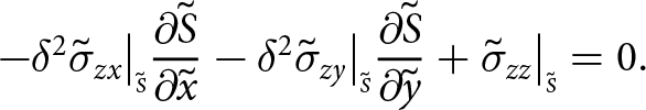 \begin{align}
-\delta^2 \tilde{\sigma}_{zx}\big|_{\scriptscriptstyle \tilde{S}}{\frac{\partial{\tilde{S}}}{\partial{\tilde{x}}}} -\delta^2 \tilde{\sigma}_{zy}\big|_{\scriptscriptstyle \tilde{S}}{\frac{\partial{\tilde{S}}}{\partial{\tilde{y}}}}+ \tilde{\sigma}_{zz}\big|_{\scriptscriptstyle \tilde{S}} &= 0.
\end{align}
\begin{align}
-\delta^2 \tilde{\sigma}_{zx}\big|_{\scriptscriptstyle \tilde{S}}{\frac{\partial{\tilde{S}}}{\partial{\tilde{x}}}} -\delta^2 \tilde{\sigma}_{zy}\big|_{\scriptscriptstyle \tilde{S}}{\frac{\partial{\tilde{S}}}{\partial{\tilde{y}}}}+ \tilde{\sigma}_{zz}\big|_{\scriptscriptstyle \tilde{S}} &= 0.
\end{align}The condition on the underside becomes
 \begin{align}
\tilde{\sigma}_{xx}\big|_{\scriptscriptstyle \tilde{B}}{\frac{\partial{\tilde{B}}}{\partial{\tilde{x}}}} +\tilde{\sigma}_{xy}\big|_{\scriptscriptstyle \tilde{B}}{\frac{\partial{\tilde{B}}}{\partial{\tilde{y}}}} - \tilde{\sigma}_{xz}\big|_{\scriptscriptstyle \tilde{B}} &= -\frac{\rho_w}{\rho_i } \tilde{B}{\frac{\partial{\tilde{B}}}{\partial{\tilde{x}}}}
\end{align}
\begin{align}
\tilde{\sigma}_{xx}\big|_{\scriptscriptstyle \tilde{B}}{\frac{\partial{\tilde{B}}}{\partial{\tilde{x}}}} +\tilde{\sigma}_{xy}\big|_{\scriptscriptstyle \tilde{B}}{\frac{\partial{\tilde{B}}}{\partial{\tilde{y}}}} - \tilde{\sigma}_{xz}\big|_{\scriptscriptstyle \tilde{B}} &= -\frac{\rho_w}{\rho_i } \tilde{B}{\frac{\partial{\tilde{B}}}{\partial{\tilde{x}}}}
\end{align} \begin{align}
\tilde{\sigma}_{yx}\big|_{\scriptscriptstyle \tilde{B}}{\frac{\partial{\tilde{B}}}{\partial{\tilde{x}}}} +\tilde{\sigma}_{yy}\big|_{\scriptscriptstyle \tilde{B}}{\frac{\partial{\tilde{B}}}{\partial{\tilde{y}}}}- \tilde{\sigma}_{yz}\big|_{\scriptscriptstyle \tilde{B}} &= -\frac{\rho_w}{\rho_i } \tilde{B} {\frac{\partial{\tilde{B}}}{\partial{\tilde{y}}}}
\end{align}
\begin{align}
\tilde{\sigma}_{yx}\big|_{\scriptscriptstyle \tilde{B}}{\frac{\partial{\tilde{B}}}{\partial{\tilde{x}}}} +\tilde{\sigma}_{yy}\big|_{\scriptscriptstyle \tilde{B}}{\frac{\partial{\tilde{B}}}{\partial{\tilde{y}}}}- \tilde{\sigma}_{yz}\big|_{\scriptscriptstyle \tilde{B}} &= -\frac{\rho_w}{\rho_i } \tilde{B} {\frac{\partial{\tilde{B}}}{\partial{\tilde{y}}}}
\end{align}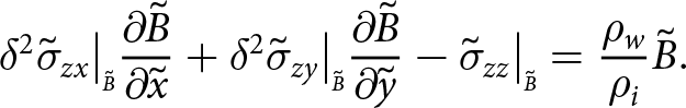 \begin{align}
\delta^2 \tilde{\sigma}_{zx}\big|_{\scriptscriptstyle \tilde{B}}{\frac{\partial{\tilde{B}}}{\partial{\tilde{x}}}} + \delta^2 \tilde{\sigma}_{zy}\big|_{\scriptscriptstyle \tilde{B}}{\frac{\partial{\tilde{B}}}{\partial{\tilde{y}}}} - \tilde{\sigma}_{zz}\big|_{\scriptscriptstyle \tilde{B}} &= \frac{\rho_w}{\rho_i } \tilde{B}.
\end{align}
\begin{align}
\delta^2 \tilde{\sigma}_{zx}\big|_{\scriptscriptstyle \tilde{B}}{\frac{\partial{\tilde{B}}}{\partial{\tilde{x}}}} + \delta^2 \tilde{\sigma}_{zy}\big|_{\scriptscriptstyle \tilde{B}}{\frac{\partial{\tilde{B}}}{\partial{\tilde{y}}}} - \tilde{\sigma}_{zz}\big|_{\scriptscriptstyle \tilde{B}} &= \frac{\rho_w}{\rho_i } \tilde{B}.
\end{align}Finally, the condition at the front of the shelf in non-dimensional form is
 \begin{align}
\tilde{\sigma}_{xx}\big|_{\scriptscriptstyle \tilde{F}}{\frac{\partial{\tilde{F}}}{\partial{\tilde{x}}}} + \tilde{\sigma}_{xy}\big|_{\scriptscriptstyle \tilde{F}}{\frac{\partial{\tilde{F}}}{\partial{\tilde{y}}}} =
\begin{cases}
0 & \tilde{z} \gt 0 \\
-\frac{\rho_{w}}{\rho_i} \tilde{z} {\frac{\partial{\tilde{F}}}{\partial{\tilde{x}}}} & \tilde{z} \lt 0
\end{cases}
\end{align}
\begin{align}
\tilde{\sigma}_{xx}\big|_{\scriptscriptstyle \tilde{F}}{\frac{\partial{\tilde{F}}}{\partial{\tilde{x}}}} + \tilde{\sigma}_{xy}\big|_{\scriptscriptstyle \tilde{F}}{\frac{\partial{\tilde{F}}}{\partial{\tilde{y}}}} =
\begin{cases}
0 & \tilde{z} \gt 0 \\
-\frac{\rho_{w}}{\rho_i} \tilde{z} {\frac{\partial{\tilde{F}}}{\partial{\tilde{x}}}} & \tilde{z} \lt 0
\end{cases}
\end{align} \begin{align}
\tilde{\sigma}_{yx}\big|_{\scriptscriptstyle \tilde{F}}{\frac{\partial{\tilde{F}}}{\partial{\tilde{x}}}} +\tilde{\sigma}_{yy}\big|_{\scriptscriptstyle \tilde{F}}{\frac{\partial{\tilde{F}}}{\partial{\tilde{y}}}} =
\begin{cases}
0 & \tilde{z} \gt 0 \\
-\frac{\rho_{w}}{\rho_i} \tilde{z} {\frac{\partial{\tilde{F}}}{\partial{\tilde{y}}}} & \tilde{z} \lt 0
\end{cases}
\end{align}
\begin{align}
\tilde{\sigma}_{yx}\big|_{\scriptscriptstyle \tilde{F}}{\frac{\partial{\tilde{F}}}{\partial{\tilde{x}}}} +\tilde{\sigma}_{yy}\big|_{\scriptscriptstyle \tilde{F}}{\frac{\partial{\tilde{F}}}{\partial{\tilde{y}}}} =
\begin{cases}
0 & \tilde{z} \gt 0 \\
-\frac{\rho_{w}}{\rho_i} \tilde{z} {\frac{\partial{\tilde{F}}}{\partial{\tilde{y}}}} & \tilde{z} \lt 0
\end{cases}
\end{align}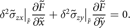 \begin{align}
\delta^2\tilde{\sigma}_{zx}\big|_{\scriptscriptstyle \tilde{F}}{\frac{\partial{\tilde{F}}}{\partial{\tilde{x}}}} +\delta^2\tilde{\sigma}_{zy}\big|_{\scriptscriptstyle \tilde{F}}{\frac{\partial{\tilde{F}}}{\partial{\tilde{y}}}} = 0.
\end{align}
\begin{align}
\delta^2\tilde{\sigma}_{zx}\big|_{\scriptscriptstyle \tilde{F}}{\frac{\partial{\tilde{F}}}{\partial{\tilde{x}}}} +\delta^2\tilde{\sigma}_{zy}\big|_{\scriptscriptstyle \tilde{F}}{\frac{\partial{\tilde{F}}}{\partial{\tilde{y}}}} = 0.
\end{align}Appendix B
The dimensionless zeroth-order terms are gathered for the boundary conditions at the surface, base and front of the shelf. The condition at the surface,
 \begin{align}
-\tilde{\sigma}_{xx}\big|_{\scriptscriptstyle \tilde{S}}{\frac{\partial{\tilde{S}}}{\partial{\tilde{x}}}} -\tilde{\sigma}_{xy}\big|_{\scriptscriptstyle \tilde{S}}{\frac{\partial{\tilde{S}}}{\partial{\tilde{y}}}}+ \tilde{\sigma}_{xz}\big|_{\scriptscriptstyle \tilde{S}} = 0
\end{align}
\begin{align}
-\tilde{\sigma}_{xx}\big|_{\scriptscriptstyle \tilde{S}}{\frac{\partial{\tilde{S}}}{\partial{\tilde{x}}}} -\tilde{\sigma}_{xy}\big|_{\scriptscriptstyle \tilde{S}}{\frac{\partial{\tilde{S}}}{\partial{\tilde{y}}}}+ \tilde{\sigma}_{xz}\big|_{\scriptscriptstyle \tilde{S}} = 0
\end{align} \begin{align}
- \tilde{\sigma}_{xy}\big|_{\scriptscriptstyle \tilde{S}}{\frac{\partial{\tilde{S}}}{\partial{\tilde{x}}}} -\tilde{\sigma}_{yy}\big|_{\scriptscriptstyle \tilde{S}}{\frac{\partial{\tilde{S}}}{\partial{\tilde{y}}}}+ \tilde{\sigma}_{yz}\big|_{\scriptscriptstyle \tilde{S}} = 0
\end{align}
\begin{align}
- \tilde{\sigma}_{xy}\big|_{\scriptscriptstyle \tilde{S}}{\frac{\partial{\tilde{S}}}{\partial{\tilde{x}}}} -\tilde{\sigma}_{yy}\big|_{\scriptscriptstyle \tilde{S}}{\frac{\partial{\tilde{S}}}{\partial{\tilde{y}}}}+ \tilde{\sigma}_{yz}\big|_{\scriptscriptstyle \tilde{S}} = 0
\end{align} \begin{align}
\tilde{\sigma}_{zz}\big|_{\scriptscriptstyle \tilde{S}} = 0
\end{align}
\begin{align}
\tilde{\sigma}_{zz}\big|_{\scriptscriptstyle \tilde{S}} = 0
\end{align}at the base,
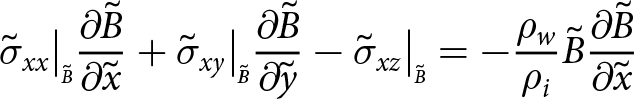 \begin{align}
\tilde{\sigma}_{xx}\big|_{\scriptscriptstyle \tilde{B}}{\frac{\partial{\tilde{B}}}{\partial{\tilde{x}}}} +\tilde{\sigma}_{xy}\big|_{\scriptscriptstyle \tilde{B}}{\frac{\partial{\tilde{B}}}{\partial{\tilde{y}}}} - \tilde{\sigma}_{xz}\big|_{\scriptscriptstyle \tilde{B}} &= -\frac{\rho_w}{\rho_i } \tilde{B}{\frac{\partial{\tilde{B}}}{\partial{\tilde{x}}}}
\end{align}
\begin{align}
\tilde{\sigma}_{xx}\big|_{\scriptscriptstyle \tilde{B}}{\frac{\partial{\tilde{B}}}{\partial{\tilde{x}}}} +\tilde{\sigma}_{xy}\big|_{\scriptscriptstyle \tilde{B}}{\frac{\partial{\tilde{B}}}{\partial{\tilde{y}}}} - \tilde{\sigma}_{xz}\big|_{\scriptscriptstyle \tilde{B}} &= -\frac{\rho_w}{\rho_i } \tilde{B}{\frac{\partial{\tilde{B}}}{\partial{\tilde{x}}}}
\end{align}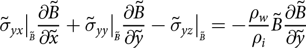 \begin{align}
\tilde{\sigma}_{yx}\big|_{\scriptscriptstyle \tilde{B}}{\frac{\partial{\tilde{B}}}{\partial{\tilde{x}}}} +\tilde{\sigma}_{yy}\big|_{\scriptscriptstyle \tilde{B}}{\frac{\partial{\tilde{B}}}{\partial{\tilde{y}}}}- \tilde{\sigma}_{yz}\big|_{\scriptscriptstyle \tilde{B}} &= -\frac{\rho_w}{\rho_i } \tilde{B} {\frac{\partial{\tilde{B}}}{\partial{\tilde{y}}}}
\end{align}
\begin{align}
\tilde{\sigma}_{yx}\big|_{\scriptscriptstyle \tilde{B}}{\frac{\partial{\tilde{B}}}{\partial{\tilde{x}}}} +\tilde{\sigma}_{yy}\big|_{\scriptscriptstyle \tilde{B}}{\frac{\partial{\tilde{B}}}{\partial{\tilde{y}}}}- \tilde{\sigma}_{yz}\big|_{\scriptscriptstyle \tilde{B}} &= -\frac{\rho_w}{\rho_i } \tilde{B} {\frac{\partial{\tilde{B}}}{\partial{\tilde{y}}}}
\end{align}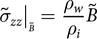 \begin{align}
\tilde{\sigma}_{zz}\big|_{\scriptscriptstyle \tilde{B}} &= \frac{\rho_w}{\rho_i } \tilde{B}
\end{align}
\begin{align}
\tilde{\sigma}_{zz}\big|_{\scriptscriptstyle \tilde{B}} &= \frac{\rho_w}{\rho_i } \tilde{B}
\end{align}and finally, at the front,
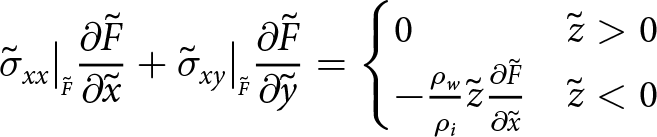 \begin{align}
\tilde{\sigma}_{xx}\big|_{\scriptscriptstyle \tilde{F}}{\frac{\partial{\tilde{F}}}{\partial{\tilde{x}}}} + \tilde{\sigma}_{xy}\big|_{\scriptscriptstyle \tilde{F}}{\frac{\partial{\tilde{F}}}{\partial{\tilde{y}}}} =
\begin{cases}
0 & \tilde{z} \gt 0 \\
-\frac{\rho_{w}}{\rho_i} \tilde{z} {\frac{\partial{\tilde{F}}}{\partial{\tilde{x}}}} & \tilde{z} \lt 0
\end{cases}
\end{align}
\begin{align}
\tilde{\sigma}_{xx}\big|_{\scriptscriptstyle \tilde{F}}{\frac{\partial{\tilde{F}}}{\partial{\tilde{x}}}} + \tilde{\sigma}_{xy}\big|_{\scriptscriptstyle \tilde{F}}{\frac{\partial{\tilde{F}}}{\partial{\tilde{y}}}} =
\begin{cases}
0 & \tilde{z} \gt 0 \\
-\frac{\rho_{w}}{\rho_i} \tilde{z} {\frac{\partial{\tilde{F}}}{\partial{\tilde{x}}}} & \tilde{z} \lt 0
\end{cases}
\end{align} \begin{align}
\tilde{\sigma}_{yx}\big|_{\scriptscriptstyle \tilde{F}}{\frac{\partial{\tilde{F}}}{\partial{\tilde{x}}}} +\tilde{\sigma}_{yy}\big|_{\scriptscriptstyle \tilde{F}}{\frac{\partial{\tilde{F}}}{\partial{\tilde{y}}}} =
\begin{cases}
0 & \tilde{z} \gt 0 \\
-\frac{\rho_{w}}{\rho_i} \tilde{z} {\frac{\partial{\tilde{F}}}{\partial{\tilde{y}}}} & \tilde{z} \lt 0
\end{cases}
\end{align}
\begin{align}
\tilde{\sigma}_{yx}\big|_{\scriptscriptstyle \tilde{F}}{\frac{\partial{\tilde{F}}}{\partial{\tilde{x}}}} +\tilde{\sigma}_{yy}\big|_{\scriptscriptstyle \tilde{F}}{\frac{\partial{\tilde{F}}}{\partial{\tilde{y}}}} =
\begin{cases}
0 & \tilde{z} \gt 0 \\
-\frac{\rho_{w}}{\rho_i} \tilde{z} {\frac{\partial{\tilde{F}}}{\partial{\tilde{y}}}} & \tilde{z} \lt 0
\end{cases}
\end{align}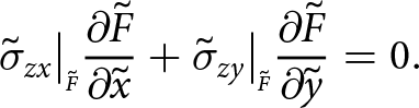 \begin{align}
\tilde{\sigma}_{zx}\big|_{\scriptscriptstyle \tilde{F}}{\frac{\partial{\tilde{F}}}{\partial{\tilde{x}}}} +\tilde{\sigma}_{zy}\big|_{\scriptscriptstyle \tilde{F}}{\frac{\partial{\tilde{F}}}{\partial{\tilde{y}}}} = 0.
\end{align}
\begin{align}
\tilde{\sigma}_{zx}\big|_{\scriptscriptstyle \tilde{F}}{\frac{\partial{\tilde{F}}}{\partial{\tilde{x}}}} +\tilde{\sigma}_{zy}\big|_{\scriptscriptstyle \tilde{F}}{\frac{\partial{\tilde{F}}}{\partial{\tilde{y}}}} = 0.
\end{align}Appendix C
This section describes the steps to obtain the SSA. The SSA approximation does not require a specific constitutive relationship but rather is reliant on incompressibility of the material description. It is included here for comparison with the steps carried out in order to obtain a plane elastic approximation (plane stress). The starting point for the SSA are the dimensionless, zeroth-order equations of momentum, Eqn (C1), in which the deviatoric stress and pressure are decomposed,
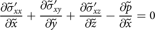 \begin{align}
{\frac{\partial{\tilde{\sigma}'_{xx}}}{\partial{\tilde{x}}}}+ {\frac{\partial{\tilde{\sigma}'_{xy}}}{\partial{\tilde{y}}}} + {\frac{\partial{\tilde{\sigma}'_{xz}}}{\partial{\tilde{z}}}}- {\frac{\partial{\tilde{p}}}{\partial{\tilde{x}}}} = 0
\end{align}
\begin{align}
{\frac{\partial{\tilde{\sigma}'_{xx}}}{\partial{\tilde{x}}}}+ {\frac{\partial{\tilde{\sigma}'_{xy}}}{\partial{\tilde{y}}}} + {\frac{\partial{\tilde{\sigma}'_{xz}}}{\partial{\tilde{z}}}}- {\frac{\partial{\tilde{p}}}{\partial{\tilde{x}}}} = 0
\end{align}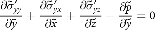 \begin{align}
{\frac{\partial{\tilde{\sigma}'_{yy}}}{\partial{\tilde{y}}}}+ {\frac{\partial{\tilde{\sigma}'_{yx}}}{\partial{\tilde{x}}}} + {\frac{\partial{\tilde{\sigma}'_{yz}}}{\partial{\tilde{z}}}} - {\frac{\partial{\tilde{p}}}{\partial{\tilde{y}}}} = 0
\end{align}
\begin{align}
{\frac{\partial{\tilde{\sigma}'_{yy}}}{\partial{\tilde{y}}}}+ {\frac{\partial{\tilde{\sigma}'_{yx}}}{\partial{\tilde{x}}}} + {\frac{\partial{\tilde{\sigma}'_{yz}}}{\partial{\tilde{z}}}} - {\frac{\partial{\tilde{p}}}{\partial{\tilde{y}}}} = 0
\end{align}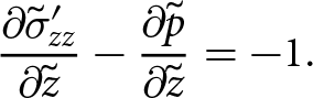 \begin{align}
{\frac{\partial{\tilde{\sigma}'_{zz}}}{\partial{\tilde{z}}}} - {\frac{\partial{\tilde{p}}}{\partial{\tilde{z}}}} = -1.
\end{align}
\begin{align}
{\frac{\partial{\tilde{\sigma}'_{zz}}}{\partial{\tilde{z}}}} - {\frac{\partial{\tilde{p}}}{\partial{\tilde{z}}}} = -1.
\end{align}The upper surface of the shelf conditions, with the same decomposition,
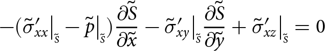 \begin{align}
-(\tilde{\sigma}'_{xx}\big|_{\scriptscriptstyle \tilde{S}}- \tilde{p}\big|_{\scriptscriptstyle \tilde{S}}){\frac{\partial{\tilde{S}}}{\partial{\tilde{x}}}} -\tilde{\sigma}'_{xy}\big|_{\scriptscriptstyle \tilde{S}}{\frac{\partial{\tilde{S}}}{\partial{\tilde{y}}}}+ \tilde{\sigma}'_{xz}\big|_{\scriptscriptstyle \tilde{S}} = 0
\end{align}
\begin{align}
-(\tilde{\sigma}'_{xx}\big|_{\scriptscriptstyle \tilde{S}}- \tilde{p}\big|_{\scriptscriptstyle \tilde{S}}){\frac{\partial{\tilde{S}}}{\partial{\tilde{x}}}} -\tilde{\sigma}'_{xy}\big|_{\scriptscriptstyle \tilde{S}}{\frac{\partial{\tilde{S}}}{\partial{\tilde{y}}}}+ \tilde{\sigma}'_{xz}\big|_{\scriptscriptstyle \tilde{S}} = 0
\end{align}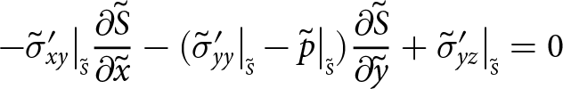 \begin{align}
- \tilde{\sigma}'_{xy}\big|_{\scriptscriptstyle \tilde{S}}{\frac{\partial{\tilde{S}}}{\partial{\tilde{x}}}} -(\tilde{\sigma}'_{yy}\big|_{\scriptscriptstyle \tilde{S}}- \tilde{p}\big|_{\scriptscriptstyle \tilde{S}}){\frac{\partial{\tilde{S}}}{\partial{\tilde{y}}}}+ \tilde{\sigma}'_{yz}\big|_{\scriptscriptstyle \tilde{S}} = 0
\end{align}
\begin{align}
- \tilde{\sigma}'_{xy}\big|_{\scriptscriptstyle \tilde{S}}{\frac{\partial{\tilde{S}}}{\partial{\tilde{x}}}} -(\tilde{\sigma}'_{yy}\big|_{\scriptscriptstyle \tilde{S}}- \tilde{p}\big|_{\scriptscriptstyle \tilde{S}}){\frac{\partial{\tilde{S}}}{\partial{\tilde{y}}}}+ \tilde{\sigma}'_{yz}\big|_{\scriptscriptstyle \tilde{S}} = 0
\end{align}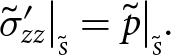 \begin{align}
\tilde{\sigma}'_{zz}\big|_{\scriptscriptstyle \tilde{S}} = \tilde{p}\big|_{\scriptscriptstyle \tilde{S}}.
\end{align}
\begin{align}
\tilde{\sigma}'_{zz}\big|_{\scriptscriptstyle \tilde{S}} = \tilde{p}\big|_{\scriptscriptstyle \tilde{S}}.
\end{align}Using the last line, pressure at the surface can be replaced into the other two directions, remembering that  $\tilde{\sigma}'_{xx}+\tilde{\sigma}'_{yy}+\tilde{\sigma}'_{zz} = 0$,
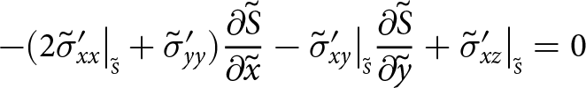 \begin{align}
-(2\tilde{\sigma}'_{xx}\big|_{\scriptscriptstyle \tilde{S}}+\tilde{\sigma}'_{yy}){\frac{\partial{\tilde{S}}}{\partial{\tilde{x}}}} -\tilde{\sigma}'_{xy}\big|_{\scriptscriptstyle \tilde{S}}{\frac{\partial{\tilde{S}}}{\partial{\tilde{y}}}}+ \tilde{\sigma}'_{xz}\big|_{\scriptscriptstyle \tilde{S}} = 0
\end{align}
\begin{align}
-(2\tilde{\sigma}'_{xx}\big|_{\scriptscriptstyle \tilde{S}}+\tilde{\sigma}'_{yy}){\frac{\partial{\tilde{S}}}{\partial{\tilde{x}}}} -\tilde{\sigma}'_{xy}\big|_{\scriptscriptstyle \tilde{S}}{\frac{\partial{\tilde{S}}}{\partial{\tilde{y}}}}+ \tilde{\sigma}'_{xz}\big|_{\scriptscriptstyle \tilde{S}} = 0
\end{align}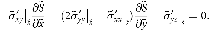 \begin{align}
- \tilde{\sigma}'_{xy}\big|_{\scriptscriptstyle \tilde{S}}{\frac{\partial{\tilde{S}}}{\partial{\tilde{x}}}} -(2\tilde{\sigma}'_{yy}\big|_{\scriptscriptstyle \tilde{S}}-\tilde{\sigma}'_{xx}\big|_{\scriptscriptstyle \tilde{S}}){\frac{\partial{\tilde{S}}}{\partial{\tilde{y}}}}+ \tilde{\sigma}'_{yz}\big|_{\scriptscriptstyle \tilde{S}} = 0.
\end{align}
\begin{align}
- \tilde{\sigma}'_{xy}\big|_{\scriptscriptstyle \tilde{S}}{\frac{\partial{\tilde{S}}}{\partial{\tilde{x}}}} -(2\tilde{\sigma}'_{yy}\big|_{\scriptscriptstyle \tilde{S}}-\tilde{\sigma}'_{xx}\big|_{\scriptscriptstyle \tilde{S}}){\frac{\partial{\tilde{S}}}{\partial{\tilde{y}}}}+ \tilde{\sigma}'_{yz}\big|_{\scriptscriptstyle \tilde{S}} = 0.
\end{align}The underside of the shelf conditions becomes
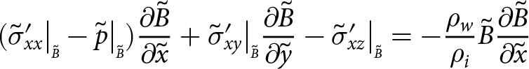 \begin{align}
(\tilde{\sigma}'_{xx}\big|_{\scriptscriptstyle \tilde{B}}- \tilde{p}\big|_{\scriptscriptstyle \tilde{B}}){\frac{\partial{\tilde{B}}}{\partial{\tilde{x}}}} +\tilde{\sigma}'_{xy}\big|_{\scriptscriptstyle \tilde{B}}{\frac{\partial{\tilde{B}}}{\partial{\tilde{y}}}} - \tilde{\sigma}'_{xz}\big|_{\scriptscriptstyle \tilde{B}} = -\frac{\rho_w}{\rho_i } \tilde{B}{\frac{\partial{\tilde{B}}}{\partial{\tilde{x}}}}
\end{align}
\begin{align}
(\tilde{\sigma}'_{xx}\big|_{\scriptscriptstyle \tilde{B}}- \tilde{p}\big|_{\scriptscriptstyle \tilde{B}}){\frac{\partial{\tilde{B}}}{\partial{\tilde{x}}}} +\tilde{\sigma}'_{xy}\big|_{\scriptscriptstyle \tilde{B}}{\frac{\partial{\tilde{B}}}{\partial{\tilde{y}}}} - \tilde{\sigma}'_{xz}\big|_{\scriptscriptstyle \tilde{B}} = -\frac{\rho_w}{\rho_i } \tilde{B}{\frac{\partial{\tilde{B}}}{\partial{\tilde{x}}}}
\end{align}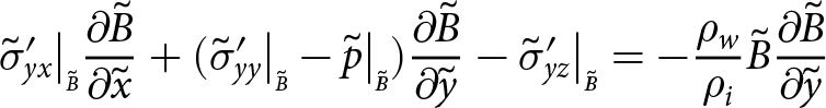 \begin{align}
\tilde{\sigma}'_{yx}\big|_{\scriptscriptstyle \tilde{B}}{\frac{\partial{\tilde{B}}}{\partial{\tilde{x}}}} +(\tilde{\sigma}'_{yy}\big|_{\scriptscriptstyle \tilde{B}}- \tilde{p}\big|_{\scriptscriptstyle \tilde{B}}){\frac{\partial{\tilde{B}}}{\partial{\tilde{y}}}}- \tilde{\sigma}'_{yz}\big|_{\scriptscriptstyle \tilde{B}} = -\frac{\rho_w}{\rho_i } \tilde{B} {\frac{\partial{\tilde{B}}}{\partial{\tilde{y}}}}
\end{align}
\begin{align}
\tilde{\sigma}'_{yx}\big|_{\scriptscriptstyle \tilde{B}}{\frac{\partial{\tilde{B}}}{\partial{\tilde{x}}}} +(\tilde{\sigma}'_{yy}\big|_{\scriptscriptstyle \tilde{B}}- \tilde{p}\big|_{\scriptscriptstyle \tilde{B}}){\frac{\partial{\tilde{B}}}{\partial{\tilde{y}}}}- \tilde{\sigma}'_{yz}\big|_{\scriptscriptstyle \tilde{B}} = -\frac{\rho_w}{\rho_i } \tilde{B} {\frac{\partial{\tilde{B}}}{\partial{\tilde{y}}}}
\end{align}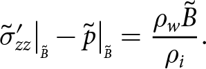 \begin{align}
\tilde{\sigma}'_{zz}\big|_{\scriptscriptstyle \tilde{B}}- \tilde{p}\big|_{\scriptscriptstyle \tilde{B}} = \frac{\rho_w \tilde{B}}{\rho_i }.
\end{align}
\begin{align}
\tilde{\sigma}'_{zz}\big|_{\scriptscriptstyle \tilde{B}}- \tilde{p}\big|_{\scriptscriptstyle \tilde{B}} = \frac{\rho_w \tilde{B}}{\rho_i }.
\end{align}This can also be simplified by solving for  $\tilde{p}$ in the last line and then inserting it back into the other two directions to obtain
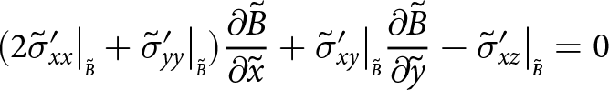 \begin{align}
(2\tilde{\sigma}'_{xx}\big|_{\scriptscriptstyle \tilde{B}} + \tilde{\sigma}'_{yy}\big|_{\scriptscriptstyle \tilde{B}}){\frac{\partial{\tilde{B}}}{\partial{\tilde{x}}}} +\tilde{\sigma}'_{xy}\big|_{\scriptscriptstyle \tilde{B}}{\frac{\partial{\tilde{B}}}{\partial{\tilde{y}}}} - \tilde{\sigma}'_{xz}\big|_{\scriptscriptstyle \tilde{B}} = 0
\end{align}
\begin{align}
(2\tilde{\sigma}'_{xx}\big|_{\scriptscriptstyle \tilde{B}} + \tilde{\sigma}'_{yy}\big|_{\scriptscriptstyle \tilde{B}}){\frac{\partial{\tilde{B}}}{\partial{\tilde{x}}}} +\tilde{\sigma}'_{xy}\big|_{\scriptscriptstyle \tilde{B}}{\frac{\partial{\tilde{B}}}{\partial{\tilde{y}}}} - \tilde{\sigma}'_{xz}\big|_{\scriptscriptstyle \tilde{B}} = 0
\end{align}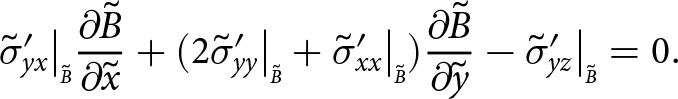 \begin{align}
\tilde{\sigma}'_{yx}\big|_{\scriptscriptstyle \tilde{B}}{\frac{\partial{\tilde{B}}}{\partial{\tilde{x}}}} +(2\tilde{\sigma}'_{yy}\big|_{\scriptscriptstyle \tilde{B}} + \tilde{\sigma}'_{xx}\big|_{\scriptscriptstyle \tilde{B}}){\frac{\partial{\tilde{B}}}{\partial{\tilde{y}}}}- \tilde{\sigma}'_{yz}\big|_{\scriptscriptstyle \tilde{B}} = 0.
\end{align}
\begin{align}
\tilde{\sigma}'_{yx}\big|_{\scriptscriptstyle \tilde{B}}{\frac{\partial{\tilde{B}}}{\partial{\tilde{x}}}} +(2\tilde{\sigma}'_{yy}\big|_{\scriptscriptstyle \tilde{B}} + \tilde{\sigma}'_{xx}\big|_{\scriptscriptstyle \tilde{B}}){\frac{\partial{\tilde{B}}}{\partial{\tilde{y}}}}- \tilde{\sigma}'_{yz}\big|_{\scriptscriptstyle \tilde{B}} = 0.
\end{align}Now a more general simplification can be made vertically integrating (C1c). Then, a general depth relation for the pressure is obtained from
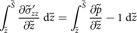 \begin{equation}
\int_{{\tilde{z}}}^{{\tilde{S}}} {{\frac{\partial{\tilde{\sigma}'_{zz}}}{\partial{\tilde{z}}}}} \: \mathrm{d}{\tilde{z}} = \int_{{\tilde{z}}}^{{\tilde{S}}} {{\frac{\partial{\tilde{p}}}{\partial{\tilde{z}}}} - 1} \: \mathrm{d}{\tilde{z}}
\end{equation}
\begin{equation}
\int_{{\tilde{z}}}^{{\tilde{S}}} {{\frac{\partial{\tilde{\sigma}'_{zz}}}{\partial{\tilde{z}}}}} \: \mathrm{d}{\tilde{z}} = \int_{{\tilde{z}}}^{{\tilde{S}}} {{\frac{\partial{\tilde{p}}}{\partial{\tilde{z}}}} - 1} \: \mathrm{d}{\tilde{z}}
\end{equation}which evaluates to
 \begin{equation}
\tilde{\sigma}'_{zz}\big|_{\scriptscriptstyle \tilde{S}} - \tilde{\sigma}'_{zz}(\tilde{z}) = \tilde{p}(\tilde{S}) - \tilde{p}(\tilde{z}) - \tilde{S} + \tilde{z}.
\end{equation}
\begin{equation}
\tilde{\sigma}'_{zz}\big|_{\scriptscriptstyle \tilde{S}} - \tilde{\sigma}'_{zz}(\tilde{z}) = \tilde{p}(\tilde{S}) - \tilde{p}(\tilde{z}) - \tilde{S} + \tilde{z}.
\end{equation}This last equation can be rearranged,
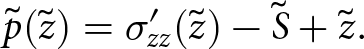 \begin{equation}
\tilde{p}(\tilde{z}) = \sigma'_{zz}(\tilde{z}) - \tilde{S} + \tilde{z}.
\end{equation}
\begin{equation}
\tilde{p}(\tilde{z}) = \sigma'_{zz}(\tilde{z}) - \tilde{S} + \tilde{z}.
\end{equation}Deriving in terms of x and y is useful for replacing the pressure terms in momentum balance equation,
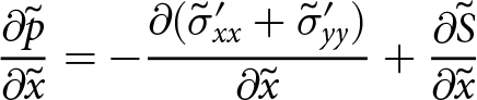 \begin{align}
{\frac{\partial{\tilde{p}}}{\partial{\tilde{x}}}} = - {\frac{\partial{(\tilde{\sigma}'_{xx} + \tilde{\sigma}'_{yy})}}{\partial{\tilde{x}}}} + {\frac{\partial{\tilde{S}}}{\partial{\tilde{x}}}}
\end{align}
\begin{align}
{\frac{\partial{\tilde{p}}}{\partial{\tilde{x}}}} = - {\frac{\partial{(\tilde{\sigma}'_{xx} + \tilde{\sigma}'_{yy})}}{\partial{\tilde{x}}}} + {\frac{\partial{\tilde{S}}}{\partial{\tilde{x}}}}
\end{align}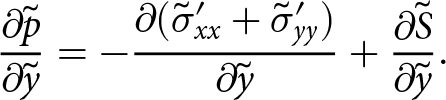 \begin{align}
{\frac{\partial{\tilde{p}}}{\partial{\tilde{y}}}} = - {\frac{\partial{(\tilde{\sigma}'_{xx} + \tilde{\sigma}'_{yy})}}{\partial{\tilde{y}}}} + {\frac{\partial{\tilde{S}}}{\partial{\tilde{y}}}}.
\end{align}
\begin{align}
{\frac{\partial{\tilde{p}}}{\partial{\tilde{y}}}} = - {\frac{\partial{(\tilde{\sigma}'_{xx} + \tilde{\sigma}'_{yy})}}{\partial{\tilde{y}}}} + {\frac{\partial{\tilde{S}}}{\partial{\tilde{y}}}}.
\end{align}Combining the above with the equations of momentum balance results in
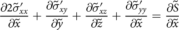 \begin{align}
{\frac{\partial{2\tilde{\sigma}'_{xx}}}{\partial{\tilde{x}}}}+ {\frac{\partial{\tilde{\sigma}'_{xy}}}{\partial{\tilde{y}}}} + {\frac{\partial{\tilde{\sigma}'_{xz}}}{\partial{\tilde{z}}}} + {\frac{\partial{\tilde{\sigma}'_{yy}}}{\partial{\tilde{x}}}} = {\frac{\partial{\tilde{S}}}{\partial{\tilde{x}}}}
\end{align}
\begin{align}
{\frac{\partial{2\tilde{\sigma}'_{xx}}}{\partial{\tilde{x}}}}+ {\frac{\partial{\tilde{\sigma}'_{xy}}}{\partial{\tilde{y}}}} + {\frac{\partial{\tilde{\sigma}'_{xz}}}{\partial{\tilde{z}}}} + {\frac{\partial{\tilde{\sigma}'_{yy}}}{\partial{\tilde{x}}}} = {\frac{\partial{\tilde{S}}}{\partial{\tilde{x}}}}
\end{align}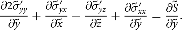 \begin{align}
{\frac{\partial{2\tilde{\sigma}'_{yy}}}{\partial{\tilde{y}}}}+ {\frac{\partial{\tilde{\sigma}'_{yx}}}{\partial{\tilde{x}}}} + {\frac{\partial{\tilde{\sigma}'_{yz}}}{\partial{\tilde{z}}}} + {\frac{\partial{\tilde{\sigma}'_{xx} }}{\partial{\tilde{y}}}} = {\frac{\partial{\tilde{S}}}{\partial{\tilde{y}}}}.
\end{align}
\begin{align}
{\frac{\partial{2\tilde{\sigma}'_{yy}}}{\partial{\tilde{y}}}}+ {\frac{\partial{\tilde{\sigma}'_{yx}}}{\partial{\tilde{x}}}} + {\frac{\partial{\tilde{\sigma}'_{yz}}}{\partial{\tilde{z}}}} + {\frac{\partial{\tilde{\sigma}'_{xx} }}{\partial{\tilde{y}}}} = {\frac{\partial{\tilde{S}}}{\partial{\tilde{y}}}}.
\end{align}Using the same vertical integration steps described in the main body of this work, the first line is integrated,
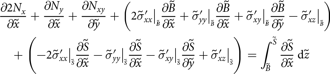 \begin{align}
&{\frac{\partial{2N_{x}}}{\partial{\tilde{x}}}} + {\frac{\partial{N_{y}}}{\partial{\tilde{x}}}} + {\frac{\partial{N_{xy}}}{\partial{\tilde{y}}}} + \left( 2\tilde{\sigma}'_{xx}\big|_{\scriptscriptstyle \tilde{B}}{\frac{\partial{\tilde{B}}}{\partial{\tilde{x}}}} + \tilde{\sigma}'_{yy}\big|_{\scriptscriptstyle \tilde{B}}{\frac{\partial{\tilde{B}}}{\partial{\tilde{x}}}} + \tilde{\sigma}'_{xy}\big|_{\scriptscriptstyle \tilde{B}}{\frac{\partial{\tilde{B}}}{\partial{\tilde{y}}}} -\tilde{\sigma}'_{xz}\big|_{\scriptscriptstyle \tilde{B}} \right) \nonumber\\
&\quad +\left(- 2\tilde{\sigma}'_{xx}\big|_{\scriptscriptstyle \tilde{S}}{\frac{\partial{\tilde{S}}}{\partial{\tilde{x}}}} - \tilde{\sigma}'_{yy}\big|_{\scriptscriptstyle \tilde{S}}{\frac{\partial{\tilde{S}}}{\partial{\tilde{x}}}} - \tilde{\sigma}'_{xy}\big|_{\scriptscriptstyle \tilde{S}}{\frac{\partial{\tilde{S}}}{\partial{\tilde{y}}}} + \tilde{\sigma}'_{xz}\big|_{\scriptscriptstyle \tilde{S}} \right) = \int_{{\tilde{B}}}^{{\tilde{S}}} {{\frac{\partial{\tilde{S}}}{\partial{\tilde{x}}}}} \: \mathrm{d}{\tilde{z}}
\end{align}
\begin{align}
&{\frac{\partial{2N_{x}}}{\partial{\tilde{x}}}} + {\frac{\partial{N_{y}}}{\partial{\tilde{x}}}} + {\frac{\partial{N_{xy}}}{\partial{\tilde{y}}}} + \left( 2\tilde{\sigma}'_{xx}\big|_{\scriptscriptstyle \tilde{B}}{\frac{\partial{\tilde{B}}}{\partial{\tilde{x}}}} + \tilde{\sigma}'_{yy}\big|_{\scriptscriptstyle \tilde{B}}{\frac{\partial{\tilde{B}}}{\partial{\tilde{x}}}} + \tilde{\sigma}'_{xy}\big|_{\scriptscriptstyle \tilde{B}}{\frac{\partial{\tilde{B}}}{\partial{\tilde{y}}}} -\tilde{\sigma}'_{xz}\big|_{\scriptscriptstyle \tilde{B}} \right) \nonumber\\
&\quad +\left(- 2\tilde{\sigma}'_{xx}\big|_{\scriptscriptstyle \tilde{S}}{\frac{\partial{\tilde{S}}}{\partial{\tilde{x}}}} - \tilde{\sigma}'_{yy}\big|_{\scriptscriptstyle \tilde{S}}{\frac{\partial{\tilde{S}}}{\partial{\tilde{x}}}} - \tilde{\sigma}'_{xy}\big|_{\scriptscriptstyle \tilde{S}}{\frac{\partial{\tilde{S}}}{\partial{\tilde{y}}}} + \tilde{\sigma}'_{xz}\big|_{\scriptscriptstyle \tilde{S}} \right) = \int_{{\tilde{B}}}^{{\tilde{S}}} {{\frac{\partial{\tilde{S}}}{\partial{\tilde{x}}}}} \: \mathrm{d}{\tilde{z}}
\end{align} in which Nx, Ny and Nxy are depth integrations of  $\tilde{\sigma}_{xx}$, $\tilde{\sigma}_{yy}$ and $\tilde{\sigma}_{xy}$. In Eqn (C11), within the first pair of large parentheses is the surface boundary condition in Eqn (C3) and within the second pair of large parenthesis, the basal boundary condition from Eqn (C5). Replacing these, Eqn (C11) becomes
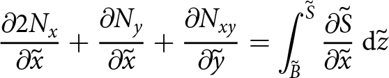 \begin{equation}
{\frac{\partial{2N_{x}}}{\partial{\tilde{x}}}} + {\frac{\partial{N_{y}}}{\partial{\tilde{x}}}} + {\frac{\partial{N_{xy}}}{\partial{\tilde{y}}}}
= \int_{{\tilde{B}}}^{{\tilde{S}}} {{\frac{\partial{\tilde{S}}}{\partial{\tilde{x}}}} } \: \mathrm{d}{\tilde{z}}
\end{equation}
\begin{equation}
{\frac{\partial{2N_{x}}}{\partial{\tilde{x}}}} + {\frac{\partial{N_{y}}}{\partial{\tilde{x}}}} + {\frac{\partial{N_{xy}}}{\partial{\tilde{y}}}}
= \int_{{\tilde{B}}}^{{\tilde{S}}} {{\frac{\partial{\tilde{S}}}{\partial{\tilde{x}}}} } \: \mathrm{d}{\tilde{z}}
\end{equation}which leads to, now including the second line,
 \begin{align}
{\frac{\partial{2N_{x}}}{\partial{\tilde{x}}}} + {\frac{\partial{N_{y}}}{\partial{\tilde{x}}}} + {\frac{\partial{N_{xy}}}{\partial{\tilde{y}}}}
= \tilde{h} {\frac{\partial{\tilde{S}}}{\partial{\tilde{x}}}}
\end{align}
\begin{align}
{\frac{\partial{2N_{x}}}{\partial{\tilde{x}}}} + {\frac{\partial{N_{y}}}{\partial{\tilde{x}}}} + {\frac{\partial{N_{xy}}}{\partial{\tilde{y}}}}
= \tilde{h} {\frac{\partial{\tilde{S}}}{\partial{\tilde{x}}}}
\end{align}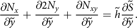 \begin{align}
{\frac{\partial{N_{x}}}{\partial{\tilde{y}}}} + {\frac{\partial{2 N_{y}}}{\partial{\tilde{y}}}} + {\frac{\partial{N_{xy}}}{\partial{\tilde{y}}}}
= \tilde{h} {\frac{\partial{\tilde{S}}}{\partial{\tilde{y}}}}.
\end{align}
\begin{align}
{\frac{\partial{N_{x}}}{\partial{\tilde{y}}}} + {\frac{\partial{2 N_{y}}}{\partial{\tilde{y}}}} + {\frac{\partial{N_{xy}}}{\partial{\tilde{y}}}}
= \tilde{h} {\frac{\partial{\tilde{S}}}{\partial{\tilde{y}}}}.
\end{align}These equations in Eqn (C13) are the SSA, for an incompressible rheology as is typically used in ice flow models.
Appendix D
In this appendix, the derivation of the plane stress approximation for the stress tensor  $\boldsymbol{\tilde{\phi}}$ is demonstrated. First, $\boldsymbol{\tilde{\sigma}}$ needs to be replaced by $\boldsymbol{\tilde{\phi}}$ in the governing equations and boundary conditions. To do this the derivative in x and y of Eqn (26) is useful,
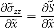 \begin{align}
{\frac{\partial{\tilde{\sigma}_{zz}}}{\partial{\tilde{x}}}} = {\frac{\partial{\tilde{S}}}{\partial{\tilde{x}}}}
\end{align}
\begin{align}
{\frac{\partial{\tilde{\sigma}_{zz}}}{\partial{\tilde{x}}}} = {\frac{\partial{\tilde{S}}}{\partial{\tilde{x}}}}
\end{align}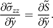 \begin{align}
{\frac{\partial{\tilde{\sigma}_{zz}}}{\partial{\tilde{y}}}} = {\frac{\partial{\tilde{S}}}{\partial{\tilde{y}}}}.
\end{align}
\begin{align}
{\frac{\partial{\tilde{\sigma}_{zz}}}{\partial{\tilde{y}}}} = {\frac{\partial{\tilde{S}}}{\partial{\tilde{y}}}}.
\end{align}The governing equations in terms of  $\tilde{\phi}$ become
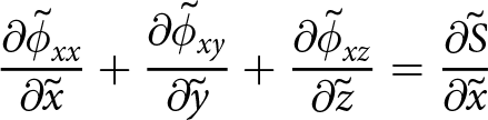 \begin{align}
{\frac{\partial{\tilde{\phi}_{xx}}}{\partial{\tilde{x}}}}+ {\frac{\partial{\tilde{\phi}_{xy}}}{\partial{\tilde{y}}}} + {\frac{\partial{\tilde{\phi}_{xz}}}{\partial{\tilde{z}}}} = {\frac{\partial{\tilde{S}}}{\partial{\tilde{x}}}}
\end{align}
\begin{align}
{\frac{\partial{\tilde{\phi}_{xx}}}{\partial{\tilde{x}}}}+ {\frac{\partial{\tilde{\phi}_{xy}}}{\partial{\tilde{y}}}} + {\frac{\partial{\tilde{\phi}_{xz}}}{\partial{\tilde{z}}}} = {\frac{\partial{\tilde{S}}}{\partial{\tilde{x}}}}
\end{align}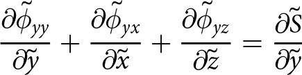 \begin{align}
{\frac{\partial{\tilde{\phi}_{yy}}}{\partial{\tilde{y}}}}+ {\frac{\partial{\tilde{\phi}_{yx}}}{\partial{\tilde{x}}}} + {\frac{\partial{\tilde{\phi}_{yz}}}{\partial{\tilde{z}}}} = {\frac{\partial{\tilde{S}}}{\partial{\tilde{y}}}}
\end{align}
\begin{align}
{\frac{\partial{\tilde{\phi}_{yy}}}{\partial{\tilde{y}}}}+ {\frac{\partial{\tilde{\phi}_{yx}}}{\partial{\tilde{x}}}} + {\frac{\partial{\tilde{\phi}_{yz}}}{\partial{\tilde{z}}}} = {\frac{\partial{\tilde{S}}}{\partial{\tilde{y}}}}
\end{align} \begin{align}
{\frac{\partial{\tilde{\phi}_{zz}}}{\partial{\tilde{z}}}} = 0.
\end{align}
\begin{align}
{\frac{\partial{\tilde{\phi}_{zz}}}{\partial{\tilde{z}}}} = 0.
\end{align}The boundary conditions become, at the surface,
 \begin{align}
-\tilde{\phi}_{xx}\big|_{\scriptscriptstyle \tilde{S}}{\frac{\partial{\tilde{S}}}{\partial{\tilde{x}}}} -\tilde{\phi}_{xy}\big|_{\scriptscriptstyle \tilde{S}}{\frac{\partial{\tilde{S}}}{\partial{\tilde{y}}}}+ \tilde{\phi}_{xz}\big|_{\scriptscriptstyle \tilde{S}} = 0
\end{align}
\begin{align}
-\tilde{\phi}_{xx}\big|_{\scriptscriptstyle \tilde{S}}{\frac{\partial{\tilde{S}}}{\partial{\tilde{x}}}} -\tilde{\phi}_{xy}\big|_{\scriptscriptstyle \tilde{S}}{\frac{\partial{\tilde{S}}}{\partial{\tilde{y}}}}+ \tilde{\phi}_{xz}\big|_{\scriptscriptstyle \tilde{S}} = 0
\end{align} \begin{align}
- \tilde{\phi}_{xy}\big|_{\scriptscriptstyle \tilde{S}}{\frac{\partial{\tilde{S}}}{\partial{\tilde{x}}}} -\tilde{\phi}_{yy}\big|_{\scriptscriptstyle \tilde{S}}{\frac{\partial{\tilde{S}}}{\partial{\tilde{y}}}}+ \tilde{\phi}_{yz}\big|_{\scriptscriptstyle \tilde{S}} = 0
\end{align}
\begin{align}
- \tilde{\phi}_{xy}\big|_{\scriptscriptstyle \tilde{S}}{\frac{\partial{\tilde{S}}}{\partial{\tilde{x}}}} -\tilde{\phi}_{yy}\big|_{\scriptscriptstyle \tilde{S}}{\frac{\partial{\tilde{S}}}{\partial{\tilde{y}}}}+ \tilde{\phi}_{yz}\big|_{\scriptscriptstyle \tilde{S}} = 0
\end{align} \begin{align}
\tilde{\phi}_{zz}\big|_{\scriptscriptstyle \tilde{S}} = 0
\end{align}
\begin{align}
\tilde{\phi}_{zz}\big|_{\scriptscriptstyle \tilde{S}} = 0
\end{align}at the base,
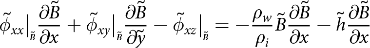 \begin{align}
\tilde{\phi}_{xx}\big|_{\scriptscriptstyle \tilde{B}}{\frac{\partial{\tilde{B}}}{\partial{x}}} +\tilde{\phi}_{xy}\big|_{\scriptscriptstyle \tilde{B}}{\frac{\partial{\tilde{B}}}{\partial{\tilde{y}}}} - \tilde{\phi}_{xz}\big|_{\scriptscriptstyle \tilde{B}} = -\frac{\rho_w}{\rho_i } \tilde{B}{\frac{\partial{\tilde{B}}}{\partial{x}}} - \tilde{h}{\frac{\partial{\tilde{B}}}{\partial{x}}}
\end{align}
\begin{align}
\tilde{\phi}_{xx}\big|_{\scriptscriptstyle \tilde{B}}{\frac{\partial{\tilde{B}}}{\partial{x}}} +\tilde{\phi}_{xy}\big|_{\scriptscriptstyle \tilde{B}}{\frac{\partial{\tilde{B}}}{\partial{\tilde{y}}}} - \tilde{\phi}_{xz}\big|_{\scriptscriptstyle \tilde{B}} = -\frac{\rho_w}{\rho_i } \tilde{B}{\frac{\partial{\tilde{B}}}{\partial{x}}} - \tilde{h}{\frac{\partial{\tilde{B}}}{\partial{x}}}
\end{align}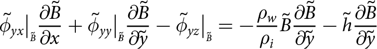 \begin{align}
\tilde{\phi}_{yx}\big|_{\scriptscriptstyle \tilde{B}}{\frac{\partial{\tilde{B}}}{\partial{x}}} +\tilde{\phi}_{yy}\big|_{\scriptscriptstyle \tilde{B}}{\frac{\partial{\tilde{B}}}{\partial{\tilde{y}}}}- \tilde{\phi}_{yz}\big|_{\scriptscriptstyle \tilde{B}} = -\frac{\rho_w}{\rho_i } \tilde{B} {\frac{\partial{\tilde{B}}}{\partial{\tilde{y}}}} - \tilde{h}{\frac{\partial{\tilde{B}}}{\partial{\tilde{y}}}}
\end{align}
\begin{align}
\tilde{\phi}_{yx}\big|_{\scriptscriptstyle \tilde{B}}{\frac{\partial{\tilde{B}}}{\partial{x}}} +\tilde{\phi}_{yy}\big|_{\scriptscriptstyle \tilde{B}}{\frac{\partial{\tilde{B}}}{\partial{\tilde{y}}}}- \tilde{\phi}_{yz}\big|_{\scriptscriptstyle \tilde{B}} = -\frac{\rho_w}{\rho_i } \tilde{B} {\frac{\partial{\tilde{B}}}{\partial{\tilde{y}}}} - \tilde{h}{\frac{\partial{\tilde{B}}}{\partial{\tilde{y}}}}
\end{align}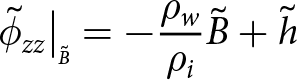 \begin{align}
\tilde{\phi}_{zz}\big|_{\scriptscriptstyle \tilde{B}} =- \frac{\rho_w}{\rho_i } \tilde{B} + \tilde{h}
\end{align}
\begin{align}
\tilde{\phi}_{zz}\big|_{\scriptscriptstyle \tilde{B}} =- \frac{\rho_w}{\rho_i } \tilde{B} + \tilde{h}
\end{align}which simplifies to
 \begin{align}
\tilde{\phi}_{xx}\big|_{\scriptscriptstyle \tilde{B}}{\frac{\partial{\tilde{B}}}{\partial{x}}} +\tilde{\phi}_{xy}\big|_{\scriptscriptstyle \tilde{B}}{\frac{\partial{\tilde{B}}}{\partial{\tilde{y}}}} - \tilde{\phi}_{xz}\big|_{\scriptscriptstyle \tilde{B}} = 0
\end{align}
\begin{align}
\tilde{\phi}_{xx}\big|_{\scriptscriptstyle \tilde{B}}{\frac{\partial{\tilde{B}}}{\partial{x}}} +\tilde{\phi}_{xy}\big|_{\scriptscriptstyle \tilde{B}}{\frac{\partial{\tilde{B}}}{\partial{\tilde{y}}}} - \tilde{\phi}_{xz}\big|_{\scriptscriptstyle \tilde{B}} = 0
\end{align}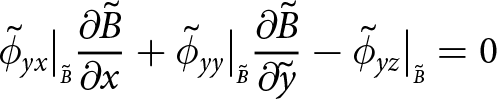 \begin{align}
\tilde{\phi}_{yx}\big|_{\scriptscriptstyle \tilde{B}}{\frac{\partial{\tilde{B}}}{\partial{x}}} +\tilde{\phi}_{yy}\big|_{\scriptscriptstyle \tilde{B}}{\frac{\partial{\tilde{B}}}{\partial{\tilde{y}}}}- \tilde{\phi}_{yz}\big|_{\scriptscriptstyle \tilde{B}} = 0
\end{align}
\begin{align}
\tilde{\phi}_{yx}\big|_{\scriptscriptstyle \tilde{B}}{\frac{\partial{\tilde{B}}}{\partial{x}}} +\tilde{\phi}_{yy}\big|_{\scriptscriptstyle \tilde{B}}{\frac{\partial{\tilde{B}}}{\partial{\tilde{y}}}}- \tilde{\phi}_{yz}\big|_{\scriptscriptstyle \tilde{B}} = 0
\end{align} \begin{align}
\tilde{\phi}_{zz}\big|_{\scriptscriptstyle \tilde{B}} =0
\end{align}
\begin{align}
\tilde{\phi}_{zz}\big|_{\scriptscriptstyle \tilde{B}} =0
\end{align}and finally, at the front,
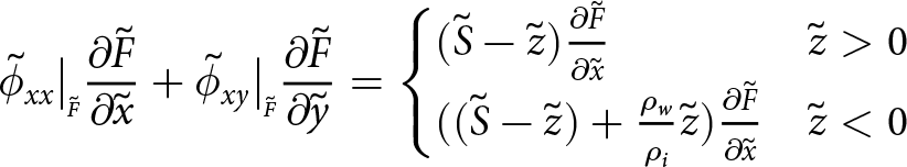 \begin{align}
\tilde{\phi}_{xx}\big|_{\scriptscriptstyle \tilde{F}}{\frac{\partial{\tilde{F}}}{\partial{\tilde{x}}}} +\tilde{\phi}_{xy}\big|_{\scriptscriptstyle \tilde{F}}{\frac{\partial{\tilde{F}}}{\partial{\tilde{y}}}} =
\begin{cases}
(\tilde{S}-\tilde{z}){\frac{\partial{\tilde{F}}}{\partial{\tilde{x}}}} & \tilde{z} \gt 0 \\
((\tilde{S}-\tilde{z}) + \frac{\rho_{w}}{\rho_i} \tilde{z}) {\frac{\partial{\tilde{F}}}{\partial{\tilde{x}}}} & \tilde{z} \lt 0
\end{cases}
\end{align}
\begin{align}
\tilde{\phi}_{xx}\big|_{\scriptscriptstyle \tilde{F}}{\frac{\partial{\tilde{F}}}{\partial{\tilde{x}}}} +\tilde{\phi}_{xy}\big|_{\scriptscriptstyle \tilde{F}}{\frac{\partial{\tilde{F}}}{\partial{\tilde{y}}}} =
\begin{cases}
(\tilde{S}-\tilde{z}){\frac{\partial{\tilde{F}}}{\partial{\tilde{x}}}} & \tilde{z} \gt 0 \\
((\tilde{S}-\tilde{z}) + \frac{\rho_{w}}{\rho_i} \tilde{z}) {\frac{\partial{\tilde{F}}}{\partial{\tilde{x}}}} & \tilde{z} \lt 0
\end{cases}
\end{align}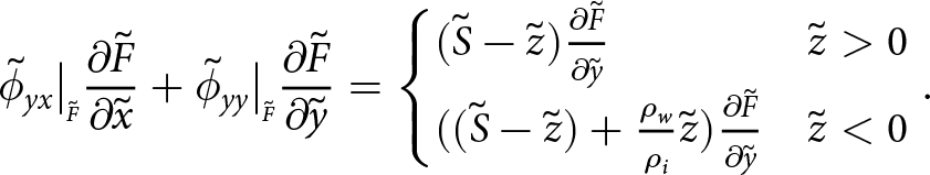 \begin{align}
\tilde{\phi}_{yx}\big|_{\scriptscriptstyle \tilde{F}}{\frac{\partial{\tilde{F}}}{\partial{\tilde{x}}}} +\tilde{\phi}_{yy}\big|_{\scriptscriptstyle \tilde{F}}{\frac{\partial{\tilde{F}}}{\partial{\tilde{y}}}} =
\begin{cases}
(\tilde{S}-\tilde{z}){\frac{\partial{\tilde{F}}}{\partial{\tilde{y}}}} & \tilde{z} \gt 0 \\
((\tilde{S}-\tilde{z}) + \frac{\rho_{w}}{\rho_i} \tilde{z}) {\frac{\partial{\tilde{F}}}{\partial{\tilde{y}}}} & \tilde{z} \lt 0
\end{cases}.
\end{align}
\begin{align}
\tilde{\phi}_{yx}\big|_{\scriptscriptstyle \tilde{F}}{\frac{\partial{\tilde{F}}}{\partial{\tilde{x}}}} +\tilde{\phi}_{yy}\big|_{\scriptscriptstyle \tilde{F}}{\frac{\partial{\tilde{F}}}{\partial{\tilde{y}}}} =
\begin{cases}
(\tilde{S}-\tilde{z}){\frac{\partial{\tilde{F}}}{\partial{\tilde{y}}}} & \tilde{z} \gt 0 \\
((\tilde{S}-\tilde{z}) + \frac{\rho_{w}}{\rho_i} \tilde{z}) {\frac{\partial{\tilde{F}}}{\partial{\tilde{y}}}} & \tilde{z} \lt 0
\end{cases}.
\end{align}The vertical integration of the momentum equation (D2) is obtained with the same approach as in the manuscript. First, vertical integration is demonstrated for  $\tilde{\phi}_{xx}$,
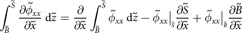 \begin{align}
\int_{{\tilde{B}}}^{{\tilde{S}}} {{\frac{\partial{\tilde{\phi}_{xx}}}{\partial{\tilde{x}}}}} \: \mathrm{d}{\tilde{z}} = \frac{\partial}{\partial{\tilde{x}}} \int_{{\tilde{B}}}^{{\tilde{S}}} {\tilde{\phi}_{xx}} \: \mathrm{d}{\tilde{z}} - \tilde{\phi}_{xx}\big|_{\scriptscriptstyle \tilde{S}} {\frac{\partial{\tilde{S}}}{\partial{\tilde{x}}}} + \tilde{\phi}_{xx}\big|_{\scriptscriptstyle \tilde{B}}{\frac{\partial{\tilde{B}}}{\partial{\tilde{x}}}}
\end{align}
\begin{align}
\int_{{\tilde{B}}}^{{\tilde{S}}} {{\frac{\partial{\tilde{\phi}_{xx}}}{\partial{\tilde{x}}}}} \: \mathrm{d}{\tilde{z}} = \frac{\partial}{\partial{\tilde{x}}} \int_{{\tilde{B}}}^{{\tilde{S}}} {\tilde{\phi}_{xx}} \: \mathrm{d}{\tilde{z}} - \tilde{\phi}_{xx}\big|_{\scriptscriptstyle \tilde{S}} {\frac{\partial{\tilde{S}}}{\partial{\tilde{x}}}} + \tilde{\phi}_{xx}\big|_{\scriptscriptstyle \tilde{B}}{\frac{\partial{\tilde{B}}}{\partial{\tilde{x}}}}
\end{align}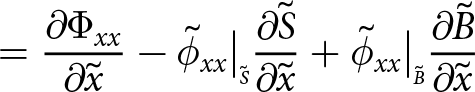 \begin{align}
\quad = {\frac{\partial{\Phi_{xx}}}{\partial{\tilde{x}}}}- \tilde{\phi}_{xx}\big|_{\scriptscriptstyle \tilde{S}}{\frac{\partial{\tilde{S}}}{\partial{\tilde{x}}}} + \tilde{\phi}_{xx}\big|_{\scriptscriptstyle \tilde{B}}{\frac{\partial{\tilde{B}}}{\partial{\tilde{x}}}}
\end{align}
\begin{align}
\quad = {\frac{\partial{\Phi_{xx}}}{\partial{\tilde{x}}}}- \tilde{\phi}_{xx}\big|_{\scriptscriptstyle \tilde{S}}{\frac{\partial{\tilde{S}}}{\partial{\tilde{x}}}} + \tilde{\phi}_{xx}\big|_{\scriptscriptstyle \tilde{B}}{\frac{\partial{\tilde{B}}}{\partial{\tilde{x}}}}
\end{align} where  $\Phi_{xx} = \int_{{\tilde{B}}}^{{\tilde{S}}} {\tilde{\phi}_{xx}} \: \mathrm{d}{\tilde{z}} $. The integration of the whole top line leads to
 \begin{align}
&{\frac{\partial{\Phi_{xx}}}{\partial{\tilde{x}}}} - \tilde{\phi}_{xx}\big|_{\scriptscriptstyle \tilde{S}}{\frac{\partial{\tilde{S}}}{\partial{\tilde{x}}}} + \tilde{\phi}_{xx}\big|_{\scriptscriptstyle \tilde{B}}{\frac{\partial{\tilde{B}}}{\partial{\tilde{x}}}} &+ {\frac{\partial{\Phi_{xy}}}{\partial{\tilde{y}}}} - \tilde{\phi}_{xy}\big|_{\scriptscriptstyle \tilde{S}}{\frac{\partial{\tilde{S}}}{\partial{\tilde{y}}}} + \tilde{\phi}_{xy}\big|_{\scriptscriptstyle \tilde{B}}{\frac{\partial{\tilde{B}}}{\partial{\tilde{y}}}} \nonumber\\
&\quad + \tilde{\phi}_{xz}\big|_{\scriptscriptstyle \tilde{S}} - \tilde{\phi}_{xz}\big|_{\scriptscriptstyle \tilde{B}} = \int_{\tilde{B}}^{\tilde{S}} {{\frac{\partial{\tilde{S}}}{\partial{\tilde{x}}}}} \:\mathrm{d}z.
\end{align}
\begin{align}
&{\frac{\partial{\Phi_{xx}}}{\partial{\tilde{x}}}} - \tilde{\phi}_{xx}\big|_{\scriptscriptstyle \tilde{S}}{\frac{\partial{\tilde{S}}}{\partial{\tilde{x}}}} + \tilde{\phi}_{xx}\big|_{\scriptscriptstyle \tilde{B}}{\frac{\partial{\tilde{B}}}{\partial{\tilde{x}}}} &+ {\frac{\partial{\Phi_{xy}}}{\partial{\tilde{y}}}} - \tilde{\phi}_{xy}\big|_{\scriptscriptstyle \tilde{S}}{\frac{\partial{\tilde{S}}}{\partial{\tilde{y}}}} + \tilde{\phi}_{xy}\big|_{\scriptscriptstyle \tilde{B}}{\frac{\partial{\tilde{B}}}{\partial{\tilde{y}}}} \nonumber\\
&\quad + \tilde{\phi}_{xz}\big|_{\scriptscriptstyle \tilde{S}} - \tilde{\phi}_{xz}\big|_{\scriptscriptstyle \tilde{B}} = \int_{\tilde{B}}^{\tilde{S}} {{\frac{\partial{\tilde{S}}}{\partial{\tilde{x}}}}} \:\mathrm{d}z.
\end{align}Reorganising in such a way that the surface and underside conditions are easily identifiable and can be used to simplify, the integration becomes
 \begin{align}
&{\frac{\partial{\Phi_{xx}}}{\partial{\tilde{x}}}} + {\frac{\partial{\Phi_{xy}}}{\partial{\tilde{y}}}} + \left( \tilde{\phi}_{xz}\big|_{\scriptscriptstyle \tilde{S}} - \tilde{\phi}_{xx}\big|_{\scriptscriptstyle \tilde{S}}{\frac{\partial{\tilde{S}}}{\partial{\tilde{x}}}} - \tilde{\phi}_{xy}\big|_{\scriptscriptstyle \tilde{S}}{\frac{\partial{\tilde{S}}}{\partial{\tilde{y}}}} \right) \nonumber\\
&\quad +\ \left( -\tilde{\phi}_{xz}\big|_{\scriptscriptstyle \tilde{B}} + \tilde{\phi}_{xx}\big|_{\scriptscriptstyle \tilde{B}}{\frac{\partial{\tilde{B}}}{\partial{\tilde{x}}}} + \tilde{\phi}_{xy}\big|_{\scriptscriptstyle \tilde{B}}{\frac{\partial{\tilde{B}}}{\partial{\tilde{y}}}} \right) = \int_{\tilde{B}}^{\tilde{S}} {{\frac{\partial{\tilde{S}}}{\partial{\tilde{x}}}}} \:\mathrm{d}z.
\end{align}
\begin{align}
&{\frac{\partial{\Phi_{xx}}}{\partial{\tilde{x}}}} + {\frac{\partial{\Phi_{xy}}}{\partial{\tilde{y}}}} + \left( \tilde{\phi}_{xz}\big|_{\scriptscriptstyle \tilde{S}} - \tilde{\phi}_{xx}\big|_{\scriptscriptstyle \tilde{S}}{\frac{\partial{\tilde{S}}}{\partial{\tilde{x}}}} - \tilde{\phi}_{xy}\big|_{\scriptscriptstyle \tilde{S}}{\frac{\partial{\tilde{S}}}{\partial{\tilde{y}}}} \right) \nonumber\\
&\quad +\ \left( -\tilde{\phi}_{xz}\big|_{\scriptscriptstyle \tilde{B}} + \tilde{\phi}_{xx}\big|_{\scriptscriptstyle \tilde{B}}{\frac{\partial{\tilde{B}}}{\partial{\tilde{x}}}} + \tilde{\phi}_{xy}\big|_{\scriptscriptstyle \tilde{B}}{\frac{\partial{\tilde{B}}}{\partial{\tilde{y}}}} \right) = \int_{\tilde{B}}^{\tilde{S}} {{\frac{\partial{\tilde{S}}}{\partial{\tilde{x}}}}} \:\mathrm{d}z.
\end{align}Simplifying by substituting the boundary conditions and now including both the first and second line, the Eqn (D2), becomes
 \begin{align}
{\frac{\partial{\Phi_{xx}}}{\partial{\tilde{x}}}} + {\frac{\partial{\Phi_{xy}}}{\partial{\tilde{y}}}} = \tilde{h} {\frac{\partial{\tilde{S}}}{\partial{\tilde{x}}}}
\end{align}
\begin{align}
{\frac{\partial{\Phi_{xx}}}{\partial{\tilde{x}}}} + {\frac{\partial{\Phi_{xy}}}{\partial{\tilde{y}}}} = \tilde{h} {\frac{\partial{\tilde{S}}}{\partial{\tilde{x}}}}
\end{align} \begin{align}
{\frac{\partial{\Phi_{yx}}}{\partial{\tilde{x}}}} + {\frac{\partial{\Phi_{yy}}}{\partial{\tilde{y}}}} = \tilde{h} {\frac{\partial{\tilde{S}}}{\partial{\tilde{y}}}}.
\end{align}
\begin{align}
{\frac{\partial{\Phi_{yx}}}{\partial{\tilde{x}}}} + {\frac{\partial{\Phi_{yy}}}{\partial{\tilde{y}}}} = \tilde{h} {\frac{\partial{\tilde{S}}}{\partial{\tilde{y}}}}.
\end{align}Equation (D11) are the governing equations of a plane elastic problem. Furthermore, this is a plane stress problem as  $\tilde{\phi}_{zz}$ is zero throughout the thickness for this order of approximation given that it is zero at the boundaries and ${\frac{\partial{\tilde{\phi}_{zz}}}{\partial{\tilde{z}}}} = 0$.
Appendix E
A 3D analytical solution, 23.1 from Tada and others Reference Tada, Paris and Irwin(1985), can be used to develop intuition about the effect of vertical variation in rift-wall loading on SIFs at a rift front. The most appropriate analytical solution available is for point loads on crack walls in an infinite, rather than finite, thickness layer. This enables the effect of the GHI to be investigated for a different geometry that is overall stiffer, due to the infinite thickness, then an ice-shelf. The point loads are used to represent the GHI, their effect is integrated over a section of the infinite planes representing opposite crack faces, of length a and height H, and a depth-dependent profile for  $K_\mathrm{I}$ is obtained for different lengths of integrated GHI. Because the GHI acts perpendicularly to the rift walls, it does not contribute to variation in $K_\mathrm{II}$ or $K_\mathrm{III}$. The following results are non-dimensional and scaled to the ice-shelf thickness, H.
The analytical result demonstrates the shape of the depth-dependence of  $K_\mathrm{I}$ SIF values (Fig. 12). SIFs are characterised by maxima at the upper and lower surfaces and a minimum close to sea level. This occurs because the GHI ‘pull’ on both rift walls is greatest at sea level, where the unopposed ice overburden is largest, and tends to zero as it approaches the upper and lower surface. The analytical $K_\mathrm{I}$ profile shapes exhibit a dependence on a that decreases with increasing a. The decreasing dependence on a suggests a limit after which conditions on the rift wall no longer influence depth-dependence of the SIFs.
Integration of the effects of point loads on the rift walls provides this expected effect of the GHI on the  $K_\mathrm{I}$ profile. The analytical expression is for an infinite medium, as shown schematically on the right, and therefore not directly comparable to an ice-shelf rift.
Appendix F
As an example of the dimensionless 3D to 2D comparison in the text, Fig. 13 shows the  $K_\mathrm{I}$ SIFs when the shelf domain is scaled so that the thickness H is 300 m.
The effect of the GHI on the  $K_\mathrm{I}$ profile for a dimensioned shelf section where $H = 300 \,\text{m}$. A symmetrical $8H \times 16H \times H$ section of shelf is used as the domain. The rift walls are loaded with the GHI, $\boldsymbol{t_{GHI}}$, and the traction at the front is purely normal to the front, ty, and equal to the mean GHI value, tG. The fracture toughness value range from Zhang and others Reference Zhang, Wang, Han, Li and Wang(2023) is plotted in teal.
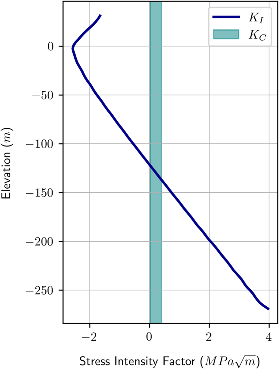
Appendix G
The same conditions presented in the comparison between 3D and 2D models are used to investigate  $K_\mathrm{III}$ SIFs (Figs 14–16). There are no comparable results from 2D models as there are admissible out-of-plane displacements.
Depth profiles of  $K_\mathrm{III}$ at the front of a rift in a symmetrical $8H \times 16H \times H$ section of shelf. The rift walls are loaded with the GHI, tG. The traction at the front, $\boldsymbol{t_F}$ has only a component normal to the front, ty, which is equal to $Y \times t_G$, where $Y = 1,2,3$ for plots from left to right.

Depth profiles of  $K_\mathrm{III}$ at the front of a rift in a symmetrical $8H \times 16H \times H$ section of shelf. The rift walls are loaded with the GHI, tG. The traction at the front, $\boldsymbol{t_F}$ has only a component tangent to the front, tx, which is $X \times t_G$, where $X = 0.2,0.4,0.6$ for plots from left to right.
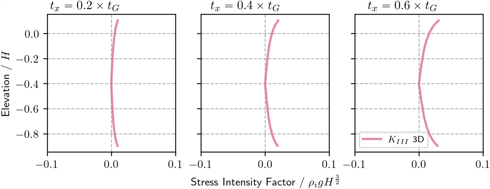
Depth profiles of  $K_\mathrm{III}$ at the front of a rift in a symmetrical $8H \times 16H \times H$ section of shelf. The rift walls are not loaded with the GHI. The traction at the front, $\boldsymbol{t_F}$ has only a component normal to the front, ty, which is equal to $Y \times t_G$, where $Y = 1,2,3$ for plots from left to right.
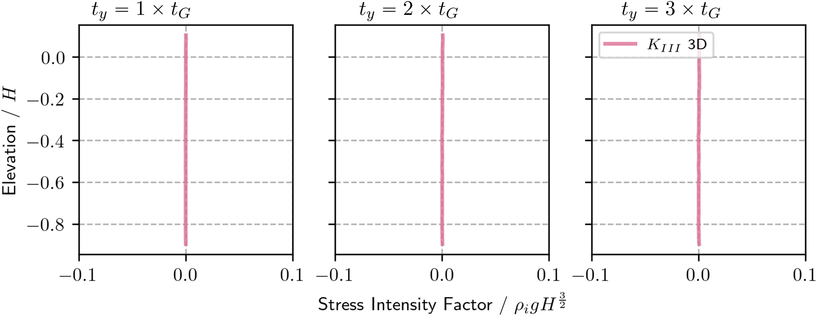


 Open access