


Impact Statement
Simulation models, and in particular, physics-driven simulation models, underpin design and maintenance across several disciplines in the built environment. Practicing engineers use these models as core engines to predict the behavior of a physical asset, such as a building or a tunnel, or to compute cost functions in optimization, or as forward models while solving inverse problems. Complex simulation models used on real-world projects can depend on a large number of parameters. These parameters describe attributes of the real-world asset, such as its materials, cross-section properties, or support conditions, and control the behavior of the simulation model. Not all parameters are created equal; there are often a small minority that are disproportionately influential compared with the rest. Being able to identify these influential parameters can make a significant difference to the outcomes of the design or optimization task that an engineer is interested in solving. Global sensitivity analysis helps us discover influential parameters; however, it is relatively uncommon in industry workflows, not least because finding these parameters is in itself a computationally expensive task. In this work, we develop a methodology to make global sensitivity analysis practical and tractable using machine learning and high-throughput computing on a public cloud. Specifically, we propose a more efficient approach by first training a neural network surrogate of a finite element model and then performing sensitivity analysis on the surrogate, rather than directly on the simulation data as is conventionally done. Using our method, a practitioner can viably complete a sensitivity analysis in a fraction of the time and budget, both of which are tight constraints on engineering design projects, without losing accuracy in the process.
1. Introduction
In the design, construction, and maintenance of infrastructure and the built environment, reducing embodied carbon is a goal of paramount importance (World Green Building Council, 2019) to counter climate change. A reduction in carbon consumption can be achieved by optimal use of construction materials when designing new projects or by promoting retrofit and maintenance through an assessment of an existing asset. To this end, engineers rely on simulations, for instance, structural analysis or geotechnical analysis, that compute the response of a system using numerical solutions to differential equations. Using these simulations as underpinnings, they solve design and assessment tasks using techniques such as optimization, digital prototyping, back analysis, or inverse modeling. The simulation models are defined using the geometries and other input parameters that describe the system being simulated. These can range from mechanical properties of the materials, details of the boundary and support conditions, to geometries and profiles of members, parts, and components.
Sensitivity analysis, which is a technique that characterizes how variations in input parameters affect the output of a model, can play a vital role in the solution to the above problems. It can help to explore causalities in a system, to reduce its dimensionality, and to support decision-making (Rajabi Moshtaghi et al., Reference Rajabi Moshtaghi, Toloie Eshlaghy and Motadel2021. Sensitivity analysis can be broadly categorized into two main branches: local and global. Local sensitivity analysis examines how small perturbations around a fixed point in the input space affect the model output. In contrast, a global sensitivity analysis considers the entire range of input parameters simultaneously, providing a more comprehensive understanding of a model’s behavior. It can account for interactions between parameters and is suitable for models of varying complexity, including those that are nonlinear; in this sense, a global sensitivity analysis is advantageous compared with a local sensitivity analysis. Sensitivity analysis is a well-established field with a wide range of methods developed for both local and global analyses (Saltelli et al., Reference Saltelli, Ratto, Andres, Campolongo, Cariboni, Gatelli, Saisana and Tarantola2008. These include local derivative-based approaches, as well as global methods such as the Morris screening method, the Fourier Amplitude Sensitivity Test, and variance-based techniques like Sobol indices.
When solving optimization and design problems, a sensitivity analysis helps identify a subset of most input parameters that have the most influence on the response quantity of interest. During the assessment of existing structures or the construction of excavations and foundations, which can often be modeled as an inverse problem, identifying parameters that are most influential to the system’s behavior enables any remedial modification to the system to be focused on this smaller subset. This can be a critical step that dictates whether such problems can be solved at all from the perspective of economy and practicality.
Within built environment engineering workflows in the industry, numerically rigorous and robust tools for computing the sensitivities of a simulation model are relatively uncommon and, as such, engineers often resort to ad-hoc approaches or rely on engineering judgment and intuition. In this article, we investigate the use of Sobol’s method for global sensitivity analysis (GSensA) for finite element (FE) models of structural engineering and geotechnical engineering problems (we abbreviate global sensitivity analysis to GSensA to avoid confusing the reader with Oasys GSA, which we introduce in the next section). There are two main contributions of this article:
-
• We describe how we can make GSensA feasible and accessible to industry practitioners using a combination of commercial simulation software, high-performance computing on the public cloud, and machine learning-based surrogation.
-
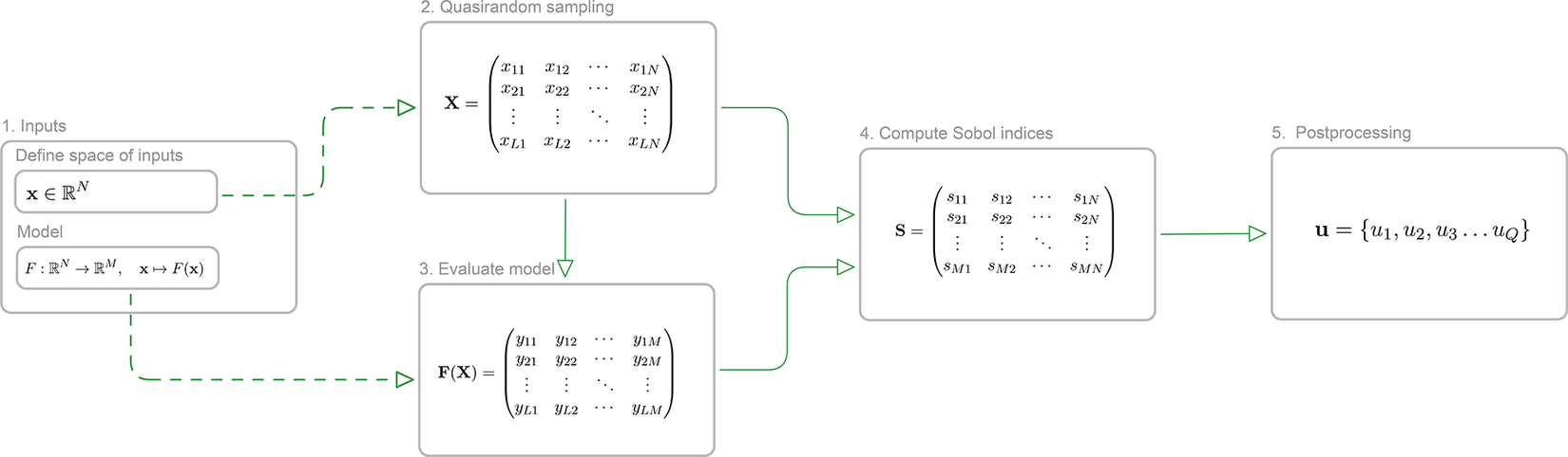
• We demonstrate, through numerical experiments, how we can alleviate the prohibitively highcomputational cost of doing a GSensA without losing fidelity of the results (Figure 1).
Schematic illustrating the workflow of Sobol analysis. Using a defined input space of parameters and a model, Sobol indices are computed using quasirandom samples. These indices are then used to identify a subset of sensitive parameters, the labels of which are denoted as $ \mathbf{u} $
.
$ \mathbf{u} $
.

2. Background
Several methods are available to compute a GSensA, and in Crusenberry et al. (Reference Crusenberry, Sobey and TerMaath2023), the authors present a comprehensive comparison of these methods. For our work, we chose the method of Soboĺ (Reference Soboĺ1993), for its relative ease of use, the maturity of the “toolset,” that is, the software ecosystem supporting the method, and its explainability to nonspecialist practitioners who would be the eventual end-users of our tool.
Sobol indices use an analysis of the variance of a function to estimate the importance of an input variable. It decomposes the variance of the model output into contributions from individual input parameters and their interactions, and computes first-order and higher-order indices. For a further summary of Sobol’s method, we refer the reader to Crusenberry et al. (Reference Crusenberry, Sobey and TerMaath2023) and Sobol (Reference Sobol2001); however, the main point of interest here is that a Sobol analysis relies on sampling the parameter space, and the number of samples needed to identify influential parameters grows with the size of the space. Since we must invoke and solve the simulation model for each realization of the sample, a GSensA using Sobol’s method has a very high computational expense and is unsuited for typical built environment design or assessment workflows. As such, the motivation for this work has been to explore how we can ameliorate the computational burden without losing the fidelity of the original analysis.
Surrogate models offer a compelling solution to this challenge by providing fast, approximate representations of complex simulations or processes. Among the various approaches, feed-forward neural networks are particularly attractive due to their ability to model highly nonlinear relationships with strong generalization capabilities. They can be trained on a dataset of high-fidelity simulation outputs and then used to make rapid predictions. Feed-forward neural networks are a type of artificial neural network where information flows in one direction—from input nodes, through hidden layers, to output nodes—without any cycles or feedback loops. Each neuron processes inputs using weighted connections and an activation function. The number of hidden layers and the number of neurons per layer are critical design choices: more layers and neurons increase the model’s capacity to capture intricate relationships, but also raise the risk of overfitting and computational cost. Their widespread adoption is supported by a mature ecosystem: neural network training is now ubiquitous, well-understood, and backed by robust, open-source software libraries such as TensorFlow and PyTorch. Advances in hardware—especially GPU acceleration and cloud computing—have made it both efficient and accessible to train these surrogate models, even for large-scale scientific and engineering applications.
There are two applications we have investigated, which originate from the disciplines of bridge engineering and ground engineering. The first is for a structural analysis of a global bridge FE model. We model the bridge in Oasys GSA, a structural analysis and design software developed by Arup (www.oasys-software.com/gsa). Oasys GSA is a Windows, desktop-based software package that encapsulates a headless modular solver for computational mechanics, which we deploy on the cloud using containerization.
The second application is a geotechnical analysis of a FE model of a retaining wall. We model this in Oasys Gofer (https://gofer.oasys-software.com/). Gofer is a cloud-native two-dimensional FE program for geotechnical analysis. Gofer encapsulates the same core FE solver as GSA, although in this case, it solves computational geomechanics problems. The Application Programming Interfaces (APIs) for either software are different and tailored for modeling workflows close to their respective disciplines.
Nevertheless, the key constraint is the computational cost as FE simulations can typically take between minutes and hours to solve, depending on model complexity, the behavior being simulated, and other factors. To resolve, we first train a machine learning surrogate from the simulations, and use this surrogate subsequently for performing the GSensA with Sobol. Since a machine learning surrogate is a black-box approximation to the behavior of the simulation model, a key question is: what is the loss of fidelity in the results? To expand, how different are the influential parameters from a Sobol using surrogates from a Sobol using the actual simulator? This is the central question we have addressed through our numerical experiments.
3. The simulation models
In this section, we detail the FE models we use for structural and geotechnical simulations. These models are inspired by real-world design and assessment projects carried out using Oasys GSA and Oasys Gofer.
3.1. Structural FE analysis
We used the global model of a 900 m span cable-stayed bridge featuring a twin-spine steel box girder deck and two monopole towers as the case study for our research (see Figure 2). The FE model was developed in Oasys GSA and has 4,508 elements, with the bridge deck modeled as two lines of spine beams connected by crossbeams, towers as beam elements, cables as cable elements, and bearings and foundations as spring elements.
GSA model of a 900-m span cable-stayed bridge (image upscaled using Microsoft Copilot v19.2509.59141.0, GPT-4).
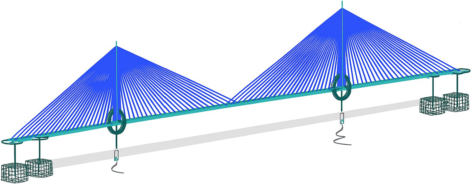
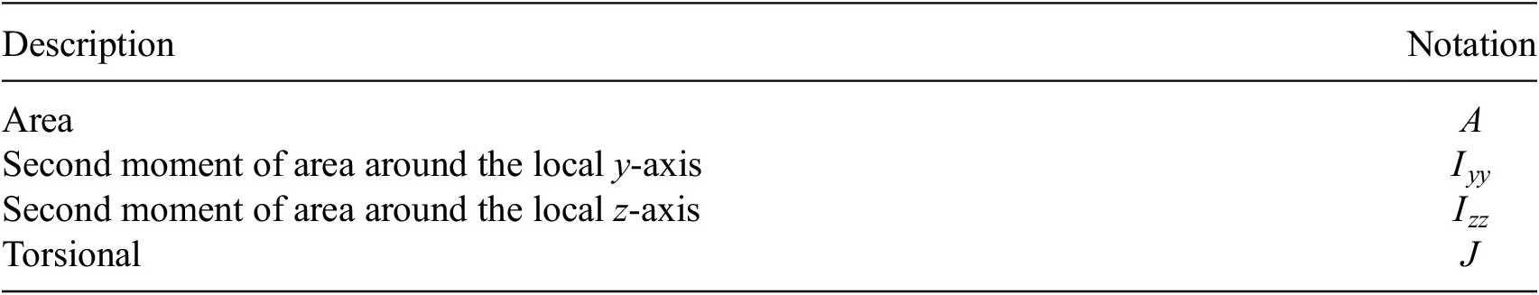
The parameters in this model are the cross-section properties of members and cables, and the stiffness of the springs. A preliminary parameter grouping is used to reduce the number of effective variables in the model. By treating a group of parameters as one, the complexity of the model is lowered, which can lead to a more efficient exploration of the parameter space for the sensitivity analysis. This grouping is done using engineering judgment (Table 1).
Notation for section modifiers used in the GSA model

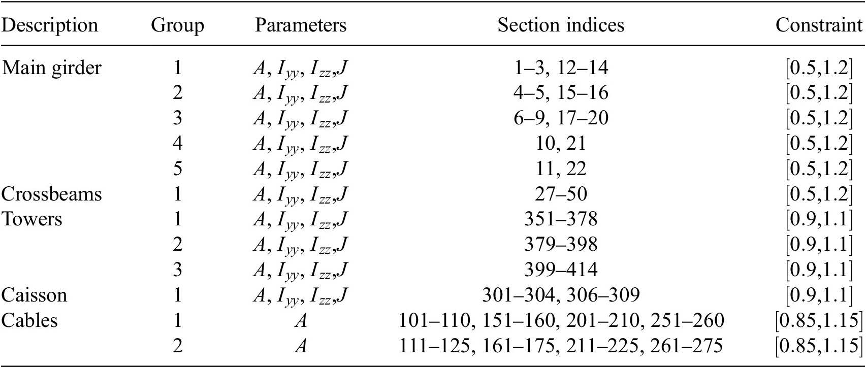
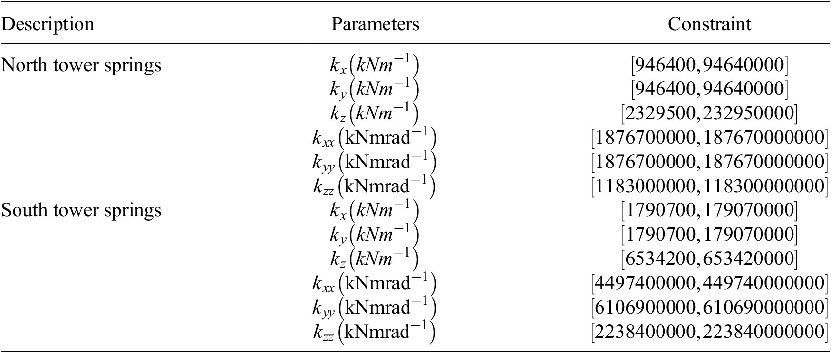
The groups and corresponding section indices in GSA are provided in Table 2. The cross-sections are modified using modification factors that are constrained as shown under the “Constraint” column. The constraints ensure a particular variable is bounded during sensitivity analysis. In addition to section modifiers, we also vary spring stiffnesses, as summarized in Table 3. In this model, the parameters in Tables 2 and 3 define the input parameter space. We consider a total of $ 54 $
input parameters and are interested in identifying their influence on the natural vibration frequencies of the structure. Since we measure the variance of the frequencies of the first
$ 54 $
input parameters and are interested in identifying their influence on the natural vibration frequencies of the structure. Since we measure the variance of the frequencies of the first $ 10 $
fundamental modes of free vibration, the simulation involves solving a modal dynamic analysis.
$ 10 $
fundamental modes of free vibration, the simulation involves solving a modal dynamic analysis.
Parameter groups and corresponding section indices for the GSA model. Constraints are applied to each parameter and are enforced during sampling

Spring stiffnesses and constraints for the GSA model. Constraints are applied to each parameter and are enforced during sampling

3.2. Geotechnical FE analysis
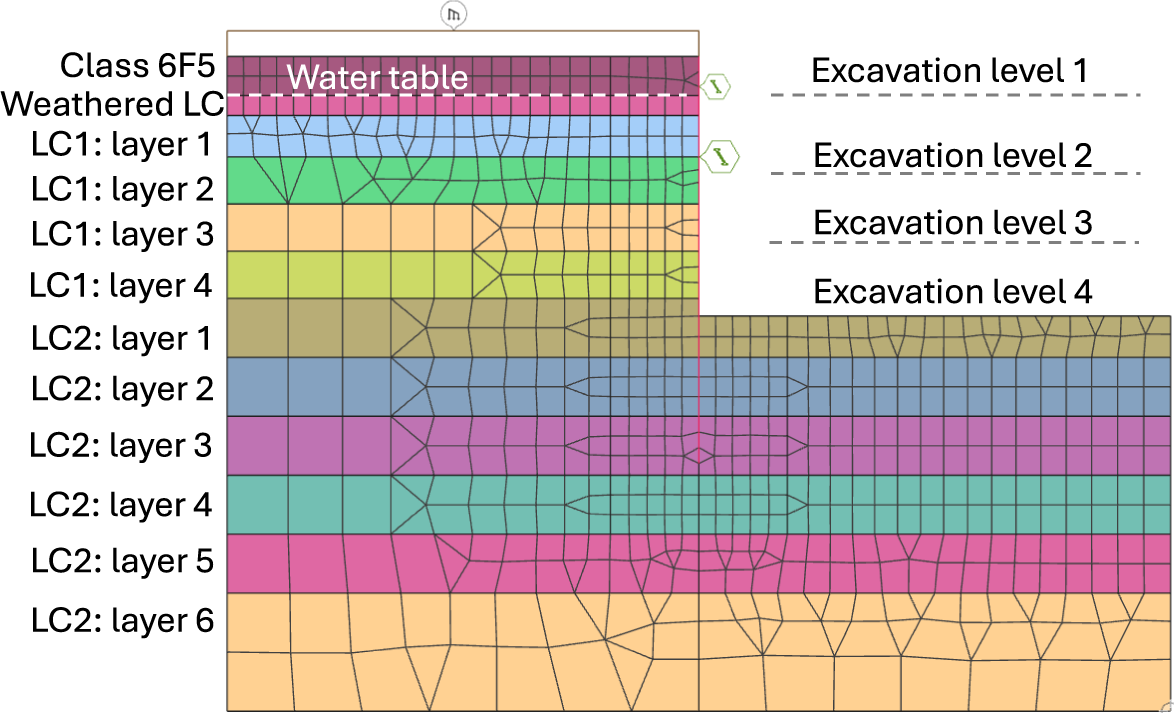
For our geotechnical case study, we modeled a 22-m deep excavation with a staged construction sequence tailored to typical Central London ground conditions (see Figure 3). The excavation was simulated using a nonlinear FE model under plane-strain conditions with Oasys Gofer. The model consists of 1,029 elements, with the soil represented by second-order quadrilateral elements, the retaining wall by beam elements, and temporary props by spring elements. The soil material behavior was modeled using a nonassociated Mohr-Coulomb (MC) failure criterion.
Schematic showing our geotechnical case study in Oasys Gofer: A 22-m deep excavation problem with a staged construction sequence tailored to typical Central London ground conditions.

The short-term construction sequence was divided into six stages, allowing us to capture variations in soil stresses and pore pressure, thereby providing the expected site deformation response. The initial stage was modeled using drained MC soil properties (i.e., effective friction angles and effective cohesions) to establish the initial site conditions before excavation. From the second stage onwards, clay soil materials were switched to undrained effective stress MC soil properties (i.e., zero friction angle and undrained shear strength values for cohesion) to capture the short-term behavior. In stage 2, a 1.2-m wide concrete retaining wall was installed along with a 10-kPa uniformly distributed load at ground level. Stage 3 involved excavating 3.3 m from the ground surface. Stage 4 included excavating 10.66 m from the ground surface and inserting the first temporary prop to support the wall. Stage 5 involved excavating 16.5 m from the ground surface and inserting a second temporary prop to support the wall. Finally, stage 6 consisted of the final excavation to a depth of 22 m from the ground surface. The ground-water table was 3.3 m below the ground surface, and the water was dewatered during the excavation.
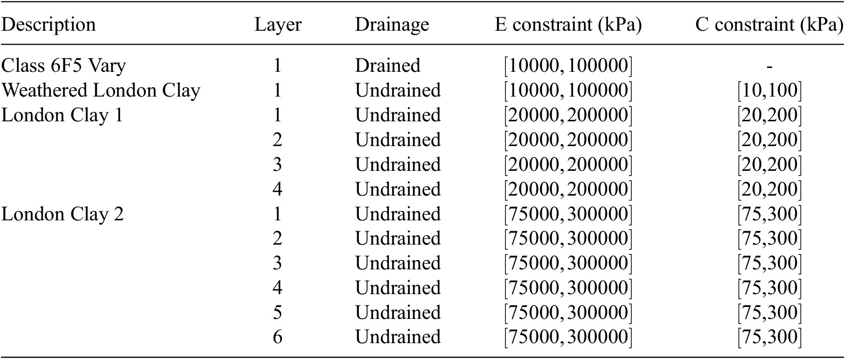
As in the structural case, engineering judgment was used to reduce the number of effective variables in the model, facilitating efficient exploration of the parameter space for the sensitivity analysis. Parameter groups for each soil layer are detailed in Table 4. The London Clay layers were subdivided into several layers to identify sensitive zones. The same set of input parameters was applied from stages 2 to 6. The outputs are the total wall displacements at the final stage.
Young’s Modulus ( $ E $
) and Cohesion (
$ E $
) and Cohesion ( $ C $
) input parameters for the Gofer model. Constraints are applied to each parameter and are enforced during sampling
$ C $
) input parameters for the Gofer model. Constraints are applied to each parameter and are enforced during sampling

4. Methodology and numerical experiments
4.1. Software implementation
Our tools are prototyped in Python and use NumPy (Harris et al., Reference Harris, Millman, Van Der Walt, Gommers, Virtanen, Cournapeau, Wieser, Taylor, Berg, Smith, Kern, Picus, Hoyer, van Kerkwijk, Brett, Haldane, Del Río, Wiebe, Peterson, Gérard-Marchant, Sheppard, Reddy, Weckesser, Abbasi, Gohlke and Oliphant2020, Numba (Lam et al., Reference Lam, Pitrou and Seibert2015, Pandas (McKinney et al., Reference McKinney2011, Pytorch (Paszke et al., Reference Paszke, Gross, Massa, Lerer, Bradbury, Chanan, Killeen, Lin, Gimelshein, Antiga, Desmaison, Kopf, Yang, DeVito, Raison, Tejani, Chilamkurthy, Steiner, Fang, Bai and Chintala2019, SALib (Herman and Usher, Reference Herman and Usher2017, and SciPy Virtanen et al., Reference Virtanen, Gommers, Oliphant, Haberland, Reddy, Cournapeau, Burovski, Peterson, Weckesser, Bright, van der Walt, Brett, Wilson, Millman, Mayorov, Nelson, Jones, Kern, Larson, Carey, Polat, Feng, Moore, VanderPlas, Laxalde, Perktold, Cimrman, Henriksen, Quintero, Harris, Archibald, Ribeiro, Pedregosa and van Mulbregt2020.
To execute and manipulate Oasys GSA models, we used its in-process API feature in Python. Analysis and manipulation of the Oasys Gofer models was performed using a purpose-built (i.e., a product feature not part of the official release) version of Oasys Gofer and a purpose-built Python API object. Each of these Python modules was then containerized using Docker (Merkel et al., Reference Merkel2014 using a Windows Server 2022 base image as the solvers to both programs are Windows-native.
4.1.1. HPC using Amazon Web Services (AWS)
The sampling for a Sobol analysis is highly computationally intensive as it involves generating quasi-random samples and executing the function, that is, the FE model, for each realization. Fortunately, this process is embarrassingly parallel and, therefore, amenable to being scaled using high-performance computing (HPC). We use AWS for parallelization. Using a public cloud provider gives us several advantages over traditional HPC supercomputing facilities or on-premise clusters, such as on-demand compute, elastic scalability, and the ability to only pay for the compute instead of investing capital expenditure upfront. We parallelized the sampling dataset generation using AWSFargate on AWS Batch, which is a highly scalable service for executing containers. Fargate is a serverless environment that abstracts away the need to manage the underlying compute infrastructure. Each Fargate instance was configured with two vCPUs and 4 GB of random access memory.
A bespoke implementation was built to trigger and orchestrate the parallel data generation. This workflow initially generates all samples sequentially on a single machine, then chunks them up based on the number of parallel container instances. Each instance processes a chunk of the samples, generates a GSA or a Gofer model for each realisation, executes the analysis, and stores the analysis results. The results from each individual container are then concatenated to produce the combined dataset of samples and corresponding simulation results. We then use AWS SageMaker to both train the surrogates using Pytorch, and subsequently run the sensitivity analysis using SALib.
4.2. Sobol analysis with surrogates
4.2.1. Creating the reference dataset
In this study, we investigate the effect of both surrogate complexity and training dataset size on the output from Sobol analysis. The accuracy of this output can be quantified by comparing the surrogate case with a reference, which we define to be the output using a large dataset obtained directly from the FE model. This reference dataset was obtained by sampling the FE model over the input space of parameters. We use SALib’s quasi-random Sobol sampler (Herman and Usher, Reference Herman and Usher2017; Renardy et al., Reference Renardy, Joslyn, Millar and Kirschner2021 to generate a uniform grid over the input parameter space. The number of samples from this method is related to the dimensionality of the parameter space $ N $
as
$ N $
as $ 2n\left(N+1\right) $
, where
$ 2n\left(N+1\right) $
, where $ n $
is a parameter controlling the density of the grid. In SALib, this should be a power of 2. We investigated output from the Sobol analysis for various values of
$ n $
is a parameter controlling the density of the grid. In SALib, this should be a power of 2. We investigated output from the Sobol analysis for various values of $ n $
and found no significant change in the output at
$ n $
and found no significant change in the output at $ n={2}^{10} $
. This value for
$ n={2}^{10} $
. This value for $ n $
was used in all subsequent sampling, with the workload parallelized over
$ n $
was used in all subsequent sampling, with the workload parallelized over $ 1000 $
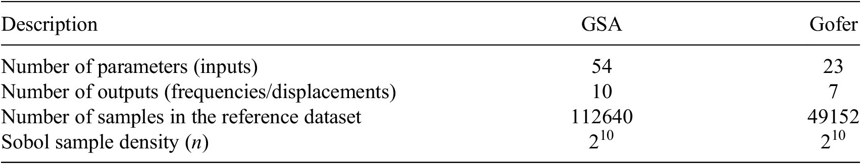
container instances. A summary of the parameters used for Sobol analysis is provided in Table 5.
$ 1000 $
container instances. A summary of the parameters used for Sobol analysis is provided in Table 5.
Summary of parameters used for Sobol analysis

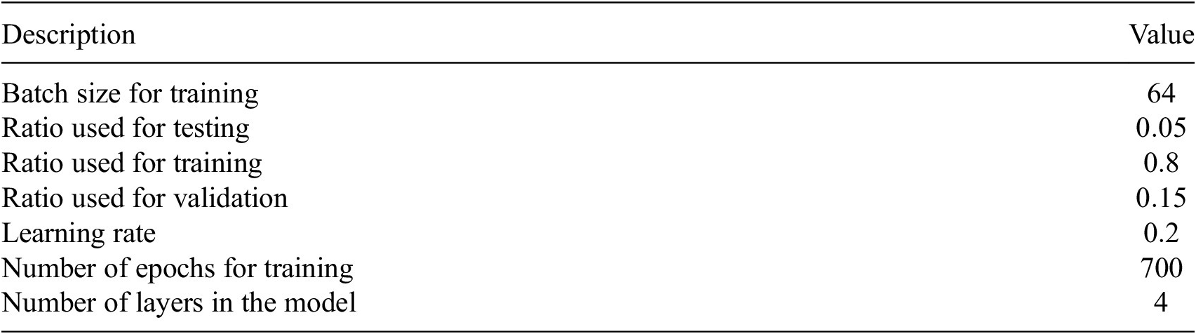
4.2.2. Training the surrogate models
We used feed-forward neural networks as surrogates to approximate the FE models. These neural networks were designed with four hidden layers and use rectified linear unit activation functions. Data for training the surrogate models was obtained by taking random subsets of the reference dataset. The percentage of data used was varied and constrained so that the minimum in the range was greater than the number of parameters in the model, to avoid overfitting. We used a maximum of $ 60\% $
reference dataset for both the GSA and Gofer surrogates, and considered
$ 60\% $
reference dataset for both the GSA and Gofer surrogates, and considered $ {N}_{pcts}^{(GSA)}=20 $
and
$ {N}_{pcts}^{(GSA)}=20 $
and $ {N}_{pcts}^{(Gofer)}=10 $
percentage values for GSA and Gofer, respectively. To obtain an averaged comparison against the reference, for a given percentage value, we require a number of trials
$ {N}_{pcts}^{(Gofer)}=10 $
percentage values for GSA and Gofer, respectively. To obtain an averaged comparison against the reference, for a given percentage value, we require a number of trials $ {N}_{trials} $
to be taken. To do this, and for each percentage value, we train
$ {N}_{trials} $
to be taken. To do this, and for each percentage value, we train $ {N}_{trials}=10 $
models using random subsets of the reference dataset. The performance of each surrogate relative to the reference output is then averaged.
$ {N}_{trials}=10 $
models using random subsets of the reference dataset. The performance of each surrogate relative to the reference output is then averaged.
We repeat this process for models of varying complexity, adjusting the number of neurons in each hidden layer of the network to modify the complexity. For the GSA surrogate, we consider $ 4 $
models with
$ 4 $
models with $ 15 $
,
$ 15 $
, $ 20 $
,
$ 20 $
, $ 35 $
, and
$ 35 $
, and $ 50 $
neurons in each hidden layer, corresponding to models with
$ 50 $
neurons in each hidden layer, corresponding to models with $ 1705 $
,
$ 1705 $
, $ 2570 $
,
$ 2570 $
, $ 6065 $
, and
$ 6065 $
, and $ 10910 $
parameters, respectively. For the Gofer surrogate, we consider
$ 10910 $
parameters, respectively. For the Gofer surrogate, we consider $ 3 $
neural nets with
$ 3 $
neural nets with $ 5 $
,
$ 5 $
, $ 8 $
, and
$ 8 $
, and $ 12 $
neurons in each hidden layer, corresponding to models with
$ 12 $
neurons in each hidden layer, corresponding to models with $ 252 $
,
$ 252 $
, $ 471 $
, and
$ 471 $
, and $ 847 $
parameters, respectively. In total, we trained
$ 847 $
parameters, respectively. In total, we trained $ {N}_{models}^{(GSA)}=800 $
and
$ {N}_{models}^{(GSA)}=800 $
and $ {N}_{models}^{(Gofer)}=300 $
models for GSA and Gofer, respectively. We compute the Sobol indices for each model according to the parameters in Table 5.
$ {N}_{models}^{(Gofer)}=300 $
models for GSA and Gofer, respectively. We compute the Sobol indices for each model according to the parameters in Table 5.

A summary of the parameters used for surrogate training is provided in Tables 6 and 7. A summary of our workflow for training surrogates is provided in Algorithm 1.
Parameters defining the scope of investigation for GSA and Gofer surrogates
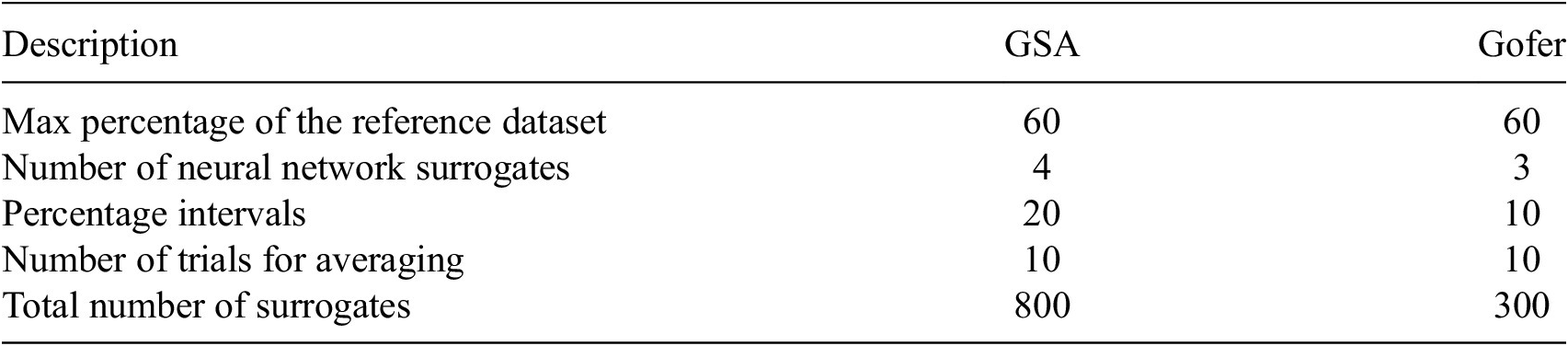
Summary of parameters used for training GSA and Gofer surrogates
4.2.3. Comparing Sobol analysis output
For a given output, SALib can calculate the first and total effects indices for each parameter, which represent the influence of that parameter on the output. We can sort these indices, from greatest to least, leading to a list of strings (the parameter names) arranged by reducing influence. This qualitative output is most relevant from a practical perspective and is, therefore, what we want to use in any comparison between FE and surrogate output. To compare the qualitative output from Sobol analysis using FE and surrogate models, we use a difference measure, which compares the lists of parameter names. A simple measure of correspondence between two rankings is to compare the ordering of elements. Let $ {\mathbf{u}}_{FE} $
and
$ {\mathbf{u}}_{FE} $
and $ {\mathbf{u}}_{surrogate} $
be the vector of parameter labels from the Sobol analysis, arranged by their corresponding Sobol indices in descending order. We assert that the elements of
$ {\mathbf{u}}_{surrogate} $
be the vector of parameter labels from the Sobol analysis, arranged by their corresponding Sobol indices in descending order. We assert that the elements of $ {\mathbf{u}}_{surrogate} $
are some permutations of
$ {\mathbf{u}}_{surrogate} $
are some permutations of $ {\mathbf{u}}_{FE} $
.
$ {\mathbf{u}}_{FE} $
.
Defining a linear elementwise operator $ \hat{P} $
, which returns the rank of a label in
$ \hat{P} $
, which returns the rank of a label in $ {\mathbf{u}}_{FE} $
, the rank difference between labels in
$ {\mathbf{u}}_{FE} $
, the rank difference between labels in $ {\mathbf{u}}_{surrogate} $
and
$ {\mathbf{u}}_{surrogate} $
and $ {\mathbf{u}}_{FE} $
is then
$ {\mathbf{u}}_{FE} $
is then
 $$ \Delta \mathbf{I}=\mathrm{abs}\left(\hat{P}{\mathbf{u}}_{FE}-\hat{P}{\mathbf{u}}_{surrogate}\right), $$
where $ \mathrm{abs}\left(\mathbf{I}\right) $
denotes the elementwise absolute value of
$ \mathrm{abs}\left(\mathbf{I}\right) $
denotes the elementwise absolute value of $ \mathbf{I} $
.
$ \mathbf{I} $
. $ \hat{P}{\mathbf{u}}_{surrogate} $
is the expected rank and
$ \hat{P}{\mathbf{u}}_{surrogate} $
is the expected rank and $ \hat{P}{\mathbf{u}}_{FE} $
is the actual rank. In order to place greater importance on the rank differences between more influential parameters, we can weight according to the first-order Sobol indices. Dividing by the largest first-order Sobol index gives an interpretable measure: it is the number of rank moves of the most sensitive parameter. We refer to this as the normalized weighted rank difference
$ \hat{P}{\mathbf{u}}_{FE} $
is the actual rank. In order to place greater importance on the rank differences between more influential parameters, we can weight according to the first-order Sobol indices. Dividing by the largest first-order Sobol index gives an interpretable measure: it is the number of rank moves of the most sensitive parameter. We refer to this as the normalized weighted rank difference
 $$ \Delta {\hat{I}}_{weighted}=\frac{{\mathbf{S}}_{\mathbf{1}}\cdot \Delta \mathbf{I}}{\max {\mathbf{S}}_{\mathbf{1}}}. $$
5. Results
5.1. Structural surrogate
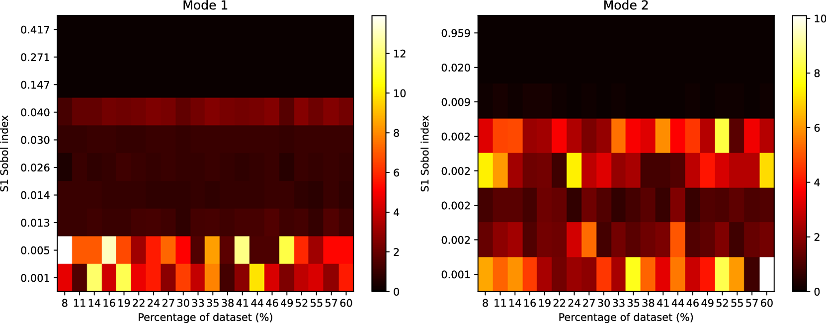
In this section, we present a series of results that compare the output from the Sobol analysis between an FE model and a surrogate trained on output from the FE model. Figure 4 shows the rank differences between GSA and the surrogate ( $ {N}_{param}=6065 $
) output. For each plot, the ordering of parameters is generally well preserved for those influential parameters with larger Sobol indices—a behavior which is found to be consistent across all training set sizes. For less influential parameters, with smaller Sobol indices, significant ordering discrepancies can be seen. This is most likely to do with “fluctuations” of order due to numerical issues, such as the number of sampling points used to compute the Sobol indices. We found no qualitative difference in these results across surrogate architectures.
$ {N}_{param}=6065 $
) output. For each plot, the ordering of parameters is generally well preserved for those influential parameters with larger Sobol indices—a behavior which is found to be consistent across all training set sizes. For less influential parameters, with smaller Sobol indices, significant ordering discrepancies can be seen. This is most likely to do with “fluctuations” of order due to numerical issues, such as the number of sampling points used to compute the Sobol indices. We found no qualitative difference in these results across surrogate architectures.
Heatmap showing the rank differences (averaged over trials) for input parameters of the GSA model. The surrogate model used here had $ 6065 $
parameters. The Sobol index for each input parameter from the FE simulation is shown on the y-axis. The percentage of the reference dataset used to train the surrogate model is shown on the x-axis. The color intensity of the heatmap represents the rank differences between the FE and surrogate output. Each panel represents these differences for each output of the model. Only Sobol indices
$ 6065 $
parameters. The Sobol index for each input parameter from the FE simulation is shown on the y-axis. The percentage of the reference dataset used to train the surrogate model is shown on the x-axis. The color intensity of the heatmap represents the rank differences between the FE and surrogate output. Each panel represents these differences for each output of the model. Only Sobol indices $ \ge {10}^{-3} $
are shown.
$ \ge {10}^{-3} $
are shown.

The effect of these fluctuations can be reduced by plotting the normalized weighted rank differences (see Section “Comparing Sobol analysis output”), which weights the rank difference according to the influence of each parameter. Plots of this measure are shown in Figure 5. No clear trend can be seen between the normalized weighted rank differences and the size of the surrogate training dataset. The rank differences are found to be consistently small across the training datasets, indicating the differences are most likely due to small fluctuations in uninfluential parameters.
Averaged normalized weighted rank differences as a function of the percentage of reference data for different GSA neural network surrogates. Each surrogate is described by $ {N}_{nn} $
parameters. Averaging was performed over parameters, outputs, and trials. The error bars are the standard error of the mean when averaged over trials. Only the lowest and highest complexity models are shown here.
$ {N}_{nn} $
parameters. Averaging was performed over parameters, outputs, and trials. The error bars are the standard error of the mean when averaged over trials. Only the lowest and highest complexity models are shown here.
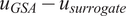
Methods of sensitivity analysis can be used for dimensionality reduction, which can, in turn, be used to improve the efficiency of computations that involve an exploration of the parameter space. From a practical perspective, the most useful output of sensitivity analysis is, therefore, the set of variables that can significantly influence a model’s behavior. This output may be post-processed and tailored for a specific use case, such as optimization, uncertainty quantification, or surrogate model training. Figure 6 shows output from the Sobol analysis, where parameters with Sobol indices $ \le 0.01 $
were excluded. Output from both the first-order and total effects indices was joined to obtain a final set of sensitive parameters.
$ \le 0.01 $
were excluded. Output from both the first-order and total effects indices was joined to obtain a final set of sensitive parameters. $ {u}_{GSA} $
and
$ {u}_{GSA} $
and $ {u}_{surrogate} $
denote the set of outputs for GSA and surrogate, respectively (it is noteworthy that unlike in Section “Comparing Sobol analysis output”, the ordering here is not important, so the vector notation has been dropped).
$ {u}_{surrogate} $
denote the set of outputs for GSA and surrogate, respectively (it is noteworthy that unlike in Section “Comparing Sobol analysis output”, the ordering here is not important, so the vector notation has been dropped). $ \mid {u}_A-{u}_B\mid $
denotes the size of the relative complement of the sets, that is, all those elements in
$ \mid {u}_A-{u}_B\mid $
denotes the size of the relative complement of the sets, that is, all those elements in $ {u}_A $
but not in
$ {u}_A $
but not in $ {u}_B $
.
$ {u}_B $
. $ {u}_{GSA}-{u}_{surrogate} $
is the set of influential parameters found when using the GSA output that were not found when using the surrogate (and vice versa).
$ {u}_{GSA}-{u}_{surrogate} $
is the set of influential parameters found when using the GSA output that were not found when using the surrogate (and vice versa).
Set differences between outputs from (post-processed) Sobol analysis for surrogates and GSA. $ {u}_{GSA} $
and
$ {u}_{GSA} $
and $ {u}_{surrogate} $
denote the set of outputs for GSA and surrogate, respectively.
$ {u}_{surrogate} $
denote the set of outputs for GSA and surrogate, respectively. $ \mid {u}_A-{u}_B\mid $
denotes the size of the set difference, that is, all those elements in
$ \mid {u}_A-{u}_B\mid $
denotes the size of the set difference, that is, all those elements in $ {u}_A $
but not in
$ {u}_A $
but not in $ {u}_B $
. Each surrogate is described by
$ {u}_B $
. Each surrogate is described by $ {N}_{nn} $
parameters. Averaging was performed over parameters, outputs, and trials. The error bars are the standard error of the mean when averaged over trials.
$ {N}_{nn} $
parameters. Averaging was performed over parameters, outputs, and trials. The error bars are the standard error of the mean when averaged over trials.
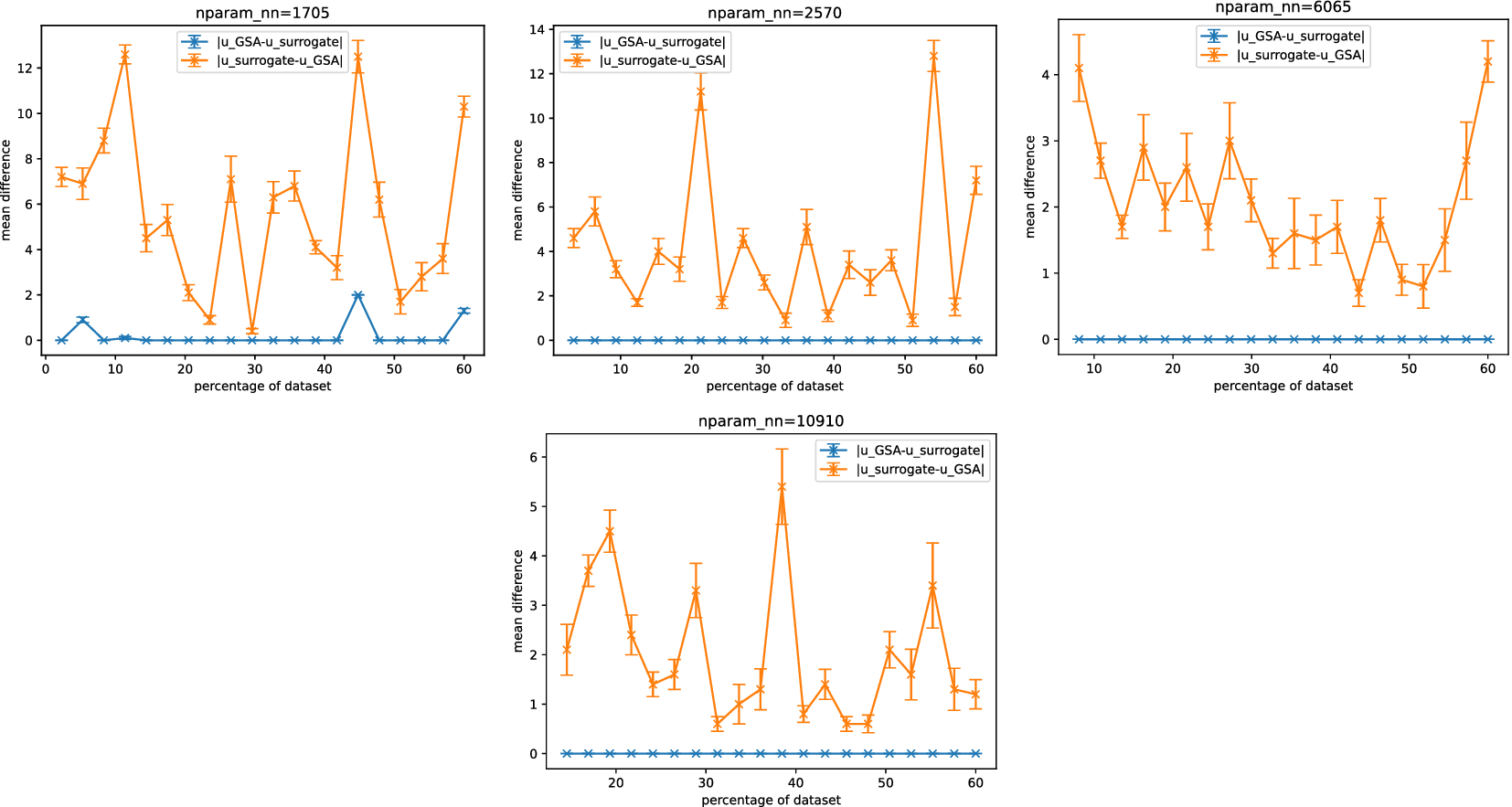
Figure 6 shows Sobol analysis with the surrogate tends to predict a larger (superset) space of sensitive parameters than in the FE case, as indicated by $ \mid {u}_{surrogate}-{u}_{GSA}\mid >0 $
and
$ \mid {u}_{surrogate}-{u}_{GSA}\mid >0 $
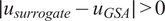
and $ \mid {u}_{GSA}-{u}_{surrogate}\mid \simeq 0 $
. Consequently, this inclusion of additional parameters may lead to reduced efficiency for any downstream computations. In the majority of surrogate architectures tested, except for the lowest complexity case, we observed that
$ \mid {u}_{GSA}-{u}_{surrogate}\mid \simeq 0 $
. Consequently, this inclusion of additional parameters may lead to reduced efficiency for any downstream computations. In the majority of surrogate architectures tested, except for the lowest complexity case, we observed that $ \mid {u}_{GSA}-{u}_{surrogate}\mid =0 $
. This indicates that Sobol analysis using the surrogate consistently identified the same sensitive parameters when using the surrogate as it did with the FE model.
$ \mid {u}_{GSA}-{u}_{surrogate}\mid =0 $
. This indicates that Sobol analysis using the surrogate consistently identified the same sensitive parameters when using the surrogate as it did with the FE model.
5.2. Geotechnical surrogate
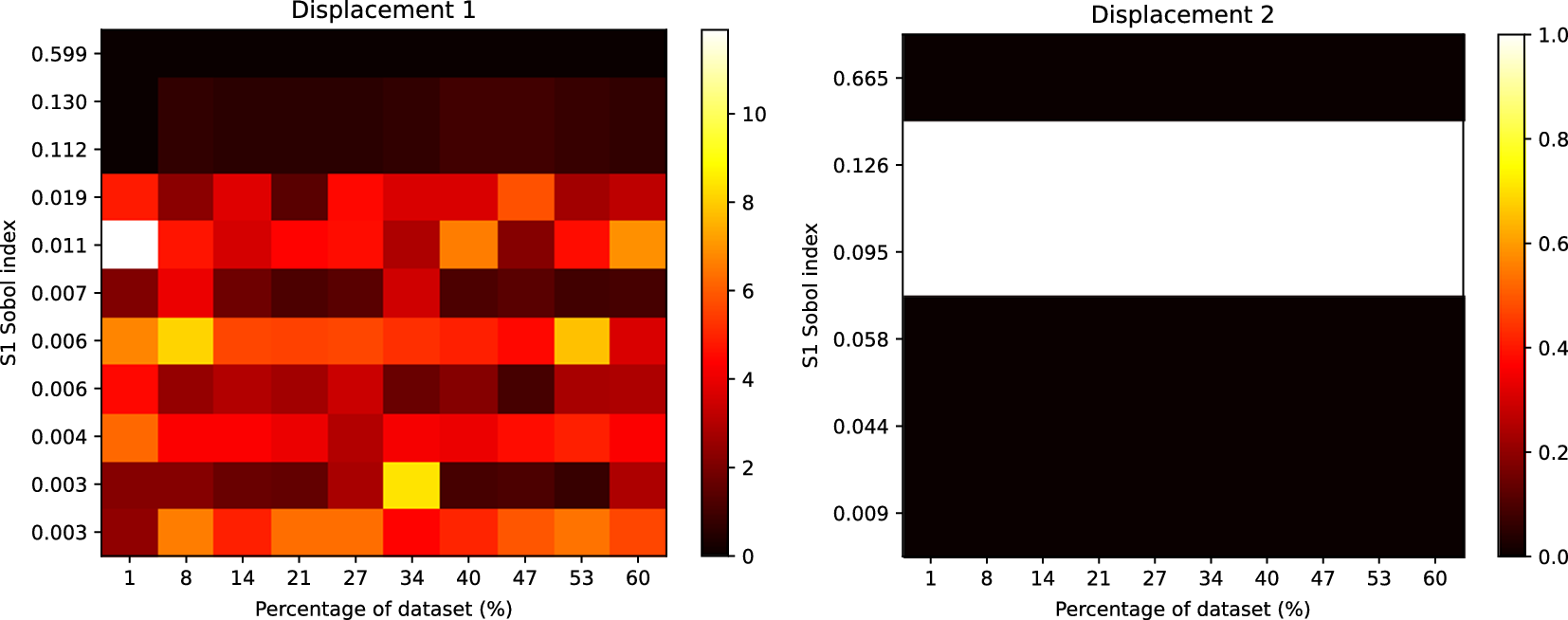
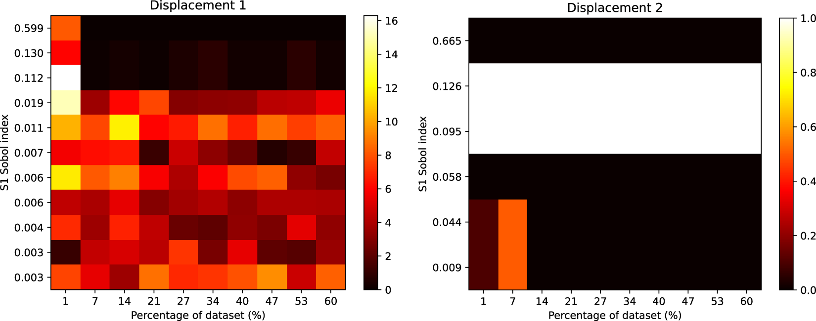
Figure 7 shows the rank differences between Gofer and surrogate ( $ {N}_{param}=471 $
) output. For each plot, we find a similar result to the GSA case, which shows the ordering of parameters to be generally well preserved for influential parameters with larger Sobol indices. With the structural model, we do not find significant rank differences for the Sobol indices approximately
$ {N}_{param}=471 $
) output. For each plot, we find a similar result to the GSA case, which shows the ordering of parameters to be generally well preserved for influential parameters with larger Sobol indices. With the structural model, we do not find significant rank differences for the Sobol indices approximately $ \ge 0.01 $
. However, for the geotechnical model, small rank discrepancies can be seen in some outputs for the Sobol indices
$ \ge 0.01 $
. However, for the geotechnical model, small rank discrepancies can be seen in some outputs for the Sobol indices $ \ge 0.01 $
, suggesting the sensitivity analysis is less reliable for the surrogate. For the lowest complexity case (
$ \ge 0.01 $
, suggesting the sensitivity analysis is less reliable for the surrogate. For the lowest complexity case ( $ {N}_{param}=252 $
), significant discrepancies can be observed in some of the outputs, particularly when the percentage of the reference dataset is small in the case of Displacement 1 (Figure 8).
$ {N}_{param}=252 $
), significant discrepancies can be observed in some of the outputs, particularly when the percentage of the reference dataset is small in the case of Displacement 1 (Figure 8).
Heatmap showing the rank differences (averaged over trials) for input parameters of the Gofer model. The surrogate model used here had $ 471 $
parameters. The Sobol index for each input parameter from the FE simulation is shown on the y-axis. The percentage of the dataset used to train the surrogate model is shown on the x-axis. The color intensity of the heatmap represents the rank differences between the FE and surrogate output. Each panel represents these differences for each output of the model. Only Sobol indices
$ 471 $
parameters. The Sobol index for each input parameter from the FE simulation is shown on the y-axis. The percentage of the dataset used to train the surrogate model is shown on the x-axis. The color intensity of the heatmap represents the rank differences between the FE and surrogate output. Each panel represents these differences for each output of the model. Only Sobol indices $ \ge {10}^{-3} $
are shown.
$ \ge {10}^{-3} $
are shown.

Heatmap showing the rank differences (averaged over trials) for input parameters of the Gofer model. The surrogate used here was the lowest complexity we considered, with $ 252 $
parameters. The Sobol index for each input parameter from the FE simulation is shown on the y-axis. The percentage of the dataset used to train the surrogate is shown on the x-axis. The colour intensity of the heatmap represents the rank differences between the FE and surrogate output. Each panel represents these differences for each output of the model. Only Sobol indices
$ 252 $
parameters. The Sobol index for each input parameter from the FE simulation is shown on the y-axis. The percentage of the dataset used to train the surrogate is shown on the x-axis. The colour intensity of the heatmap represents the rank differences between the FE and surrogate output. Each panel represents these differences for each output of the model. Only Sobol indices $ \ge {10}^{-3} $
are shown.
$ \ge {10}^{-3} $
are shown.

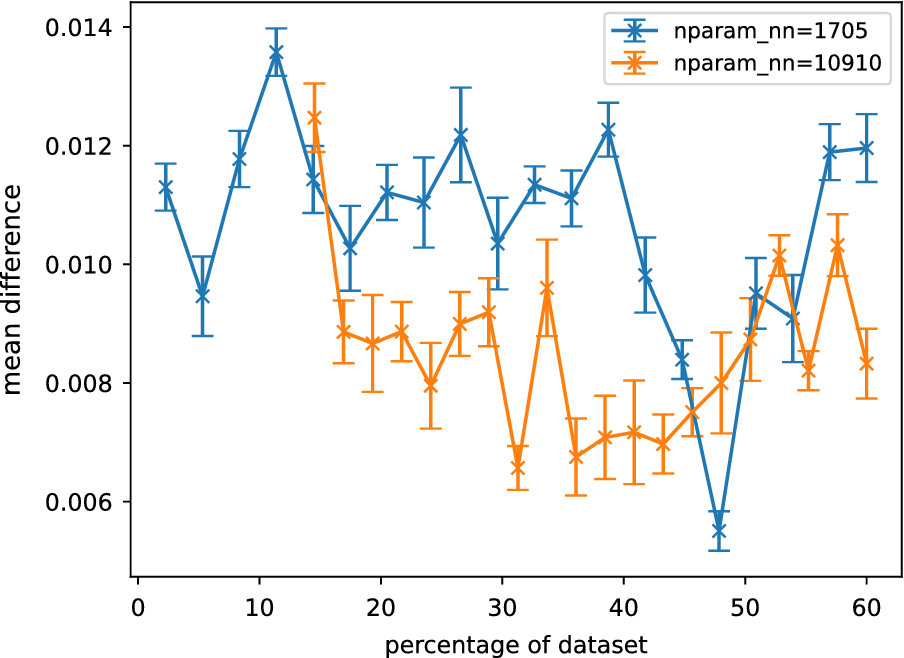
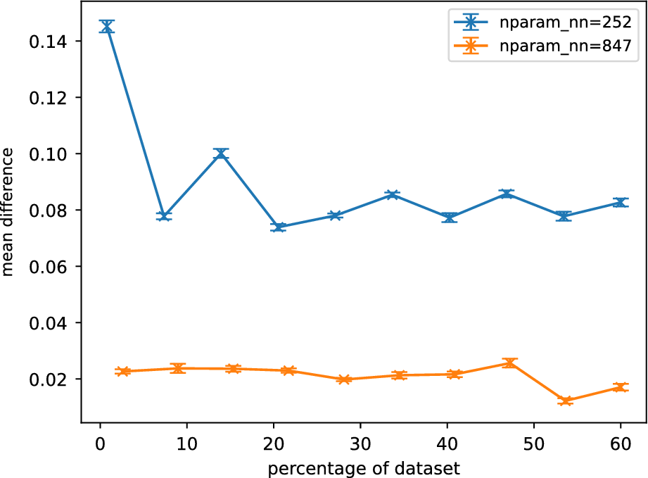
Figure 9 shows the averaged normalized weighted rank differences for surrogates of different sizes. A clear trend can be seen for $ {N}_{nn}=252 $
, where increasing training data benefits the accuracy of the sensitivity analysis. For the larger neural nets, this trend is less clear. The larger surrogates are also found to perform better in the sensitivity analysis.
$ {N}_{nn}=252 $
, where increasing training data benefits the accuracy of the sensitivity analysis. For the larger neural nets, this trend is less clear. The larger surrogates are also found to perform better in the sensitivity analysis.
Averaged normalized weighted rank differences as a function of percentage of training data for different Gofer surrogates. Each surrogate is described by $ {N}_{nn} $
parameters. Averaging was performed over parameters, outputs, and trials. The error bars are the standard error of the mean when averaged over trials. Only the lowest and highest complexity models are shown here.
$ {N}_{nn} $
parameters. Averaging was performed over parameters, outputs, and trials. The error bars are the standard error of the mean when averaged over trials. Only the lowest and highest complexity models are shown here.

The increased difficulty in training surrogates for Gofer is likely to originate from inherent nonlinearity in the MC material model. These behaviors include sharp gradients and discontinuities in the response of the FE model, making it challenging for neural networks to generalize accurately across the input space. In contrast, the modal analysis of the GSA model, which is linear elastic, typically exhibits smoother and more globally linear behavior. This makes the surrogate learning task more tractable, as the mapping from input parameters to outputs is more stable and predictable.
6. Conclusion
Our study using Sobol analysis with neural network surrogates reveals several key insights. First, we have shown that, in the case of GSA and Gofer, the ordering of influential parameters with larger Sobol indices is generally well preserved across all training set sizes and model complexities investigated. This indicates the surrogate model’s reliability in identifying these parameters.
However, significant discrepancies are observed for less influential parameters, likely due to numerical issues such as the number of sampling points used. This may lead to qualitatively different predictions for the set of sensitive parameters in practice, which we find in the case of GSA. In these tests, the set of sensitive parameters was found to be a superset of the FE reference case. Our results also show that accurate results from Sobol analysis can be achieved even with surrogates trained on a small fraction of the reference dataset. Model complexity appears to play a bigger role in determining the accuracy of Sobol output with surrogates, which is particularly apparent for Gofer.
One method of generating a set of sensitive parameters is to include only those parameters with Sobol indices greater than a threshold. Our results suggest that, when surrogates are used, this threshold should typically be lowered so as to minimize the chances of excluding parameters that may have otherwise been deemed sensitive had the full FE model been used.
Future work should focus on several key areas. First, it would be worth exploring the impact of sampling density on the accuracy of Sobol indices. Large sampling densities could help mitigate the numerical issues observed for less influential parameters. Finally, expanding the scope of the study to include a wider range of case studies and real-world applications would validate the generalizability of our approach and highlight its practical relevance in various domains.
Data availability statement
The data supporting this study (Weerasinghe et al., Reference Weerasinghe, Bandara, Ye and Kannan2025) are available via the Open Science Framework (Center for Open Science, 2025) at https://doi.org/10.17605/OSF.IO/HFWT8.
Author contribution
Conceptualization-Lead: G.W.; Conceptualization-Supporting: R.K.; Data curation-Lead: G.W.; Data curation-Supporting: S.B.; Formal analysis-Lead: G.W.; Formal analysis-Supporting: R.K.; Investigation-Lead: G.W.; Investigation-Supporting: R.K., S.B.; Methodology-Lead: G.W.; Methodology-Supporting: R.K., S.B.; Software-Lead: G.W.; Supervision-Lead: R.K.; Validation-Lead: G.W.; Visualization-Lead: G.W.; Visualization-Supporting: S.B.; Writing – Original Draft-Equal: R.K.; Writing – Original Draft-Lead: G.W.; Writing – Original Draft-Supporting: S.B.; Writing – Review & Editing-Equal: G.W., R.K.; Writing –Review & Editing-Supporting: S.B.
Funding statement
The authors gratefully acknowledge funding from Arup and cloud computing support from Amazon Web Services. R. Kannan would like to acknowledge funding from the Royal Academy of Engineering Industrial Fellowship.
Competing interests
The authors declare none.


 Open access
Comments
No Comments have been published for this article.