


1. Introduction
Active Galactic Nuclei (AGN) jets and their associated radio lobes are extragalactic sources of radio synchrotron emission. Since AGN jets provide an important source of feedback that regulates galaxy evolution (McNamara & Nulsen Reference McNamara and Nulsen2007; Somerville & Davé Reference Somerville and Davé2015), understanding the emission of their radio lobes is critical for interpreting the physical effect that AGN jets have on their environments. The synchrotron emission comes from high-energy electrons in AGN jets that are accelerated at shocks (e.g. Burbidge Reference Burbidge1956). These electrons undergo energy losses due to synchrotron, adiabatic, and inverse-Compton (IC) processes. The energy loss processes are dependent upon the dynamics of the jet and its cocoon. In particular, the magnitude and spatial distribution of synchrotron emission depends on the magnetic fields present in AGN jets and their cocoons.
Radio synchrotron emission from AGN jets is highly linearly polarised, with a maximum fractional polarisation of around 70% (Pacholczyk Reference Pacholczyk1970). Simulation studies of polarised radio emission from AGN jet-inflated lobes have been conducted over the past few decades (e.g. Matthews & Scheuer Reference Matthews and Scheuer1990a, b; Tregillis, Jones, & Ryu Reference Tregillis, Jones and Ryu2004; Huarte-Espinosa, Krause, & Alexander Reference Huarte-Espinosa, Krause and Alexander2011a; Hardcastle & Krause Reference Hardcastle and Krause2014; English, Hardcastle, & Krause Reference English, Hardcastle and Krause2016; Meenakshi et al. Reference Meenakshi, Mukherjee, Bodo and Rossi2023; Stimpson, Hardcastle, & Krause Reference Stimpson, Hardcastle and Krause2023). In this work, we study the polarisation properties of kpc-scale AGN jets and their associated radio lobes using 3-dimensional relativistic magnetohydrodynamical simulations.
Previous studies of the Stokes parameters in simulations of kpc-scale AGN jets by Huarte-Espinosa et al. (Reference Huarte-Espinosa, Krause and Alexander2011a), Hardcastle & Krause (Reference Hardcastle and Krause2014), and English et al. (Reference English, Hardcastle and Krause2016) calculate the synchrotron emission based on numerical grid quantities; this is the same approach as originally outlined by Matthews & Scheuer (Reference Matthews and Scheuer1990a, b), though the latter authors derived the magnetic field from simplifying assumptions using purely hydrodynamic simulations. The Stokes emissivities due to synchrotron emission are calculated in a grid-based manner based upon the magnetic field components, which are then integrated along each line of sight to create a 2-dimensional synthetic observation. This method does not account for an evolving electron energy distribution (e.g. one experiencing adiabatic and IC losses) but is a useful first step into understanding how the magnetic structure in the radio lobes influences the emission.
Meenakshi et al. (Reference Meenakshi, Mukherjee, Bodo and Rossi2023) have published the most advanced relativistic magnetohydrodynamic (RMHD) simulations of polarised radio emission in AGN jets and lobes to date. This method uses a hybrid grid and particle method by Vaidya et al. (Reference Vaidya, Mignone, Bodo, Rossi and Massaglia2018) to track the evolution of each particle as it is advected by the fluid on the simulation grid. The energy distribution of the particles is followed in situ by solving the relativistic cosmic ray transport equation. The synchrotron emissivity and full Stokes parameters are calculated within the simulations, and the surface brightness images are then ray-traced in post-processing. The authors study radio lobes of intermediate sizes of up to approximately 30 kpc in total length. This continues a tradition of in situ treatment of electrons in AGN jet simulations (e.g. Jones, Ryu, & Engel Reference Jones, Ryu and Engel1999; Tregillis et al. Reference Tregillis, Jones and Ryu2004; Jones & Kang Reference Jones and Kang2005; Nolting et al. Reference Nolting2022).
Kramer et al. (Reference Kramer, MacDonald, Paraschos and Ricci2024) use a similar method in their RMHD simulations of parsec-scale AGN jets. The authors use Lagrangian particles in their simulations and follow the energy distribution of the particles in a similar manner to Vaidya et al. (Reference Vaidya, Mignone, Bodo, Rossi and Massaglia2018), however, they post-process their simulated data (including calculating the polarised emission) using the RADMC-3D code (MacDonald & Nishikawa Reference MacDonald and Nishikawa2021). The RADMC-3D code calculates the full radiative transfer of the Stokes’ parameters as based on the methods of Jones & O’Dell (Reference Jones and O’Dell1977a, b). We do not consider the full radiative transfer of the Stokes’ parameters in this work. This hybrid method incorporates a mixture of in situ and ex situ treatments (in situ particles/energy distribution, ex situ emissivity), in contrast to a fully post-processed method (e.g. Fromm et al. Reference Fromm, Perucho, Mimica and Ros2016) or fully in situ method (e.g. Meenakshi et al. Reference Meenakshi, Mukherjee, Bodo and Rossi2023).
In this paper we introduce a new method of calculating polarised radio emission, building on the PRAiSE (Particles + Radio AGN in Semi-analytic Environments) framework (Yates-Jones et al. Reference Yates-Jones, Turner, Shabala and Krause2022; Turner et al. Reference Turner, Rogers, Shabala and Krause2018a). The PRAiSE method is also a hybrid approach, using Lagrangian particles that are advected by the fluid in a grid-based simulation to evolve the particle energy distribution and calculate synchrotron emissivity ex situ. These particles record the history of the local fluid values (pressure, density, velocity, magnetic field) encountered along their trajectory and the time since the particle last passed through a shock (using three thresholds, see Yates-Jones et al. Reference Yates-Jones, Turner, Shabala and Krause2022, for more details). The particle energy distributions and the associated synchrotron emission are calculated in post-processing, rather than within the simulation, and account for (re-)acceleration due to strong shocks, and subsequent adiabatic, synchrotron, and IC losses. The evolution of particle energy is found by interpolating the emitting particle Lorentz factor backwards in time to the last acceleration event experienced by that particle. In contrast to the methods used by Vaidya et al. (Reference Vaidya, Mignone, Bodo, Rossi and Massaglia2018) and Kramer et al. (Reference Kramer, MacDonald, Paraschos and Ricci2024), our method allows for more flexibility in our parameter choice (e.g. injection index, redshift) as the computationally efficient particle energy distribution calculation is performed in post-processing, rather than in situ.
Previously, the PRAiSE method has made the assumption that the magnetic field is proportional to the pressure in AGN jets and their lobes. In this paper, we directly use the magnetic field from RMHD simulations to calculate the radio emission, which is implemented as an extension to the PRAiSE code, which we call BRAiSE (B field + RAiSE). Since the magnetic fields in radio lobes are turbulent, the structure of the magnetic field will influence the structures seen in the radio emission (Huarte-Espinosa et al. Reference Huarte-Espinosa, Krause and Alexander2011a; Hardcastle & Krause Reference Hardcastle and Krause2014). This is seen in observations, where the intrinsic magnetic field direction follows synchrotron filaments in radio lobes (e.g. Taylor et al. Reference Taylor1990; Eilek & Owen Reference Eilek and Owen2002; Sebokolodi et al. Reference Sebokolodi2020).
We use BRAiSE to study depolarisation through calculating polarisation position angles (e.g. MacDonald & Nishikawa Reference MacDonald and Nishikawa2021; Meenakshi et al. Reference Meenakshi, Mukherjee, Bodo and Rossi2023) and Faraday depth (e.g. Jerrim et al. Reference Jerrim2024) for the radio synchrotron emission. AGN radio lobes are depolarised through Faraday rotation as the radio emission travels through a magnetoionised medium to the observer (Burn Reference Burn1966). Faraday rotation rotates the polarisation angle of the radio emission in the following way (Burn Reference Burn1966):
 \begin{equation} \chi = \chi_0 + \phi \lambda^2.\end{equation}
Here,
 $\chi_0$
is the intrinsic polarisation angle,
$\chi_0$
is the intrinsic polarisation angle,
 $\phi$
is the Faraday depth, and
$\phi$
is the Faraday depth, and
 $\lambda$
is the wavelength of the emission. The Faraday depth quantifies the amount of Faraday rotation and depends on the magnetic field strength, environment density, and line of sight to the source (Carilli & Taylor Reference Carilli and Taylor2002):
$\lambda$
is the wavelength of the emission. The Faraday depth quantifies the amount of Faraday rotation and depends on the magnetic field strength, environment density, and line of sight to the source (Carilli & Taylor Reference Carilli and Taylor2002):
 \begin{equation} \phi = 812 \int^l_0 n_e \boldsymbol{B} \cdot \textrm{d}\boldsymbol{l} \: \: \textrm{rad/m}^{2}.\end{equation}
Here, the thermal electron number density
 $n_e$
is in cm
$n_e$
is in cm
 $^{-3}$
, the magnetic field strength
$^{-3}$
, the magnetic field strength
 $\boldsymbol{B}$
is in
$\boldsymbol{B}$
is in
 $\mu$
G, and the path length
$\mu$
G, and the path length
 $\textrm{d}\boldsymbol{l}$
is in kpc. As described in Jerrim et al. (Reference Jerrim2024), we can calculate the Faraday depth from our fluid variables on the simulation grid (henceforth referred to as the rotation measure). In this work, we apply these rotation measures (RMs) to our generated synchrotron emission to directly study depolarisation by Faraday rotation in our synthetic polarised radio emission.
$\textrm{d}\boldsymbol{l}$
is in kpc. As described in Jerrim et al. (Reference Jerrim2024), we can calculate the Faraday depth from our fluid variables on the simulation grid (henceforth referred to as the rotation measure). In this work, we apply these rotation measures (RMs) to our generated synchrotron emission to directly study depolarisation by Faraday rotation in our synthetic polarised radio emission.
Depolarisation due to differential Faraday rotation can occur due to the three-dimensional nature of the radio lobe; emission from different depths throughout the lobe will have different amounts of Faraday rotation, which will randomise the polarisation angle (Burn Reference Burn1966; Sokoloff et al. Reference Sokoloff1998). However, the radio emission is also depolarised through the observing process. Within a telescope observing beam, many lines of sight to the source will be averaged over: if the polarisation of the emission or the RM structure is not uniform across the beam, this averaging will reduce the total fractional polarisation (Gabuzda Reference Gabuzda2020). This observational effect is known as beam depolarisation.
The paper is structured as follows. In Section 2, we present the differences between the equations for when we use pressure (PRAiSE) or magnetic field (BRAiSE) to calculate the radio emission. We validate our results in Section 3 by discussing the jet dynamics (Section 3.2) and then the impact of the dynamics and the emission method on the surface brightness (Section 3.3). The synthetic polarised radio images are discussed in Section 4, including an examination of depolarisation due to Faraday rotation (Section 4.2). We conclude with a summary of our findings in Section 5.
2. BRAiSE implementation
2.1 Synchrotron emission
Our synthetic radio synchrotron emission code (PRAiSE) uses the pressure of the Lagrangian tracer particles in our PLUTO simulations, mapping this to the magnetic field energy density for the synchrotron calculation. For the full details of the PRAiSE calculation, we refer the reader to Yates-Jones et al. (Reference Yates-Jones, Turner, Shabala and Krause2022) and Turner et al. (Reference Turner, Rogers, Shabala and Krause2018a). In this work, we introduce the BRAiSE extension to the radio emission code, which calculates the radio emissivities directly from the magnetic field strength of the Lagrangian tracer particles in our simulations. We also include a framework to calculate the full Stokes parameters from our simulations. Removing the assumption of mapping pressure to magnetic energy density changes the particle rest-frame emissivity per unit volume and per unit solid angle at frequency
 $\nu$
from (Equation 5 of Yates-Jones et al. Reference Yates-Jones, Turner, Shabala and Krause2022):
$\nu$
from (Equation 5 of Yates-Jones et al. Reference Yates-Jones, Turner, Shabala and Krause2022):
 \begin{align}\begin{split} J_{\nu} =\ &\frac{\kappa(s)}{4 \pi} \left( \frac{e^2}{2} \right)^{\frac{5 + s}{4}} \left( \frac{\mu_0}{(\Gamma_c - 1)} \right)^{\frac{5 + s}{4}} \left(\frac{3}{\pi}\right)^{\frac{s}{2}} \frac{1}{m_e^{\frac{3 + s}{2}} c (s+1)} \nu^\frac{1 - s}{2} \\ & \times \frac{\eta^{\frac{1+s}{4}}}{(\eta + 1)^{\frac{5+s}{4}}} p(t)^{\frac{5 + s}{4}} \left( \frac{p(t_{\rm acc})}{p(t)} \right)^{1 - \frac{4}{3 \Gamma_c}} \left(\frac{\gamma_{\rm acc}}{\gamma}\right)^{2-s} \\ & \times \left[\frac{\gamma_{\rm max}^{2-s} - \gamma_{\rm min}^{2-s}}{2 - s} - \frac{\gamma_{\rm max}^{1-s} - \gamma_{\rm min}^{1-s}}{1 - s} \right]^{-1},\end{split}\end{align}
to:
 \begin{align} \begin{split} J_{\nu} =\ &\frac{\kappa(s)}{2 \pi} \left( \frac{e^2}{4} \right)^{\frac{5 + s}{4}} \mu_0 \left(\frac{3}{\pi}\right)^\frac{s}{2} \frac{1}{m_e^{\frac{3+s}{2}} c (s+1)} \nu^\frac{1 - s}{2} \\ & \times B^{\frac{1+s}{2}} u_e(t_{\rm acc}) \left( \frac{p'(t_{\rm acc})}{p'(t)} \right)^{- \frac{4}{3 \Gamma_c}} \left(\frac{\gamma_{\rm acc}}{\gamma}\right)^{2-s} \\ & \times \left[\frac{\gamma_{\rm max}^{2-s} - \gamma_{\rm min}^{2-s}}{2 - s} - \frac{\gamma_{\rm max}^{1-s} - \gamma_{\rm min}^{1-s}}{1 - s} \right]^{-1}. \end{split}\end{align}
In these equations,
 $\Gamma_c$
is the cocoon adiabatic index, s is the electron energy power law exponent,
$\Gamma_c$
is the cocoon adiabatic index, s is the electron energy power law exponent,
 $\gamma_{\rm min}$
and
$\gamma_{\rm min}$
and
 $\gamma_{\rm max}$
are the accelerated particle Lorentz limits, and the particle Lorentz factors
$\gamma_{\rm max}$
are the accelerated particle Lorentz limits, and the particle Lorentz factors
 $\gamma$
and
$\gamma$
and
 $\gamma_{\rm acc}$
are calculated at the current time and time of particle shock acceleration, respectively.
$\gamma_{\rm acc}$
are calculated at the current time and time of particle shock acceleration, respectively.
We also have
 $p(t)$
and
$p(t)$
and
 $p(t_{acc})$
as the local particle pressures at the current time and time of particle acceleration, respectively. In Equation (3), p refers to the total pressure, which includes thermal, non-thermal, and magnetic components. However, in our numerical simulation code, the pressure variable only accounts for non-magnetic pressure. Since in PRAiSE we assume that the magnetic field scales with thermal pressure, the ratio
$p(t_{acc})$
as the local particle pressures at the current time and time of particle acceleration, respectively. In Equation (3), p refers to the total pressure, which includes thermal, non-thermal, and magnetic components. However, in our numerical simulation code, the pressure variable only accounts for non-magnetic pressure. Since in PRAiSE we assume that the magnetic field scales with thermal pressure, the ratio
 $p(t_{\rm acc})/p(t)$
will remain unchanged whether the non-magnetic or total pressure is used. This ratio comes from adiabatic expansion, which is driven by thermal pressure, so we do not include the magnetic pressure in BRAiSE; we denote the non-magnetic pressure as
$p(t_{\rm acc})/p(t)$
will remain unchanged whether the non-magnetic or total pressure is used. This ratio comes from adiabatic expansion, which is driven by thermal pressure, so we do not include the magnetic pressure in BRAiSE; we denote the non-magnetic pressure as
 $p'(t)$
. In BRAiSE, we therefore calculate the electron energy density as:
$p'(t)$
. In BRAiSE, we therefore calculate the electron energy density as:
 \begin{align} u_e(t_{\rm acc}) = \frac{p'(t_{\rm acc})}{(\Gamma_c - 1)}. \end{align}
We note that the emissivity equations appear to differ in the power of the adiabatic expansion factor, however, the equations reduce to the same result; the difference is reflected in the differing scaling constants between the two approaches. The constant
 $\kappa(s)$
is given by Longair (Reference Longair2011) to be:
$\kappa(s)$
is given by Longair (Reference Longair2011) to be:
 \begin{equation} \kappa(s) = \frac{\Gamma\big(\frac{s}{4} + \frac{19}{12}\big) \Gamma\big(\frac{s}{4} - \frac{1}{12}\big) \Gamma\big(\frac{s}{4} + \frac{5}{4}\big) }{\Gamma\big(\frac{s}{4} + \frac{7}{4}\big)}.\end{equation}
To convert between Equations (3) and (4), we define an equipartition factor
 $\eta = u_B / u_e$
as the ratio of magnetic energy density to electron energy density. Following Kaiser, Dennett-Thorpe, & Alexander (Reference Kaiser, Dennett-Thorpe and Alexander1997), we use the lobe pressure
$\eta = u_B / u_e$
as the ratio of magnetic energy density to electron energy density. Following Kaiser, Dennett-Thorpe, & Alexander (Reference Kaiser, Dennett-Thorpe and Alexander1997), we use the lobe pressure
 $p = (\Gamma_c - 1) (u_e + u_B + u_T)$
, where we assume the thermal energy density\break
$p = (\Gamma_c - 1) (u_e + u_B + u_T)$
, where we assume the thermal energy density\break
 $u_T \sim 0$
.
$u_T \sim 0$
.
We use the fluid tracer value from our numerical simulation code to define the volume filling factor of radiating particles in each Lagrangian particle packet. The tracer value is a mass tracer, defined as follows:
 \begin{align} \begin{split} {\rm trc} &= \frac{n_r m_r}{n_r m_r + n_{th} m_{ th}}, \\ \frac{n_{ th}}{n_{r}} &= \frac{m_r}{m_{th}} \left( \frac{1}{\rm trc} - 1 \right), \end{split}\end{align}
where
 $n_{r}$
is the number density of radiating particles,
$n_{r}$
is the number density of radiating particles,
 $m_{r}$
is the mass of lobe plasma associated with each radiating particle (i.e., the sum of electron mass and positively charged particle mass),
$m_{r}$
is the mass of lobe plasma associated with each radiating particle (i.e., the sum of electron mass and positively charged particle mass),
 $n_{th}$
is the number density of thermal particles, and
$n_{th}$
is the number density of thermal particles, and
 $m_{th}$
is the mass of the thermal particles. The volume filling factor then is:
$m_{th}$
is the mass of the thermal particles. The volume filling factor then is:
 \begin{equation} f = \frac{1}{1 + \frac{m_r}{m_{\rm th}} \left( \frac{1}{\rm trc} - 1 \right)}.\end{equation}
We use a mass ratio of 1, corresponding to an electron-proton plasma (as
 $m_r = m_{th} = \mu m_p$
), which simplifies this volume filling factor to a multiplication by the tracer value (following Yates-Jones et al. Reference Yates-Jones, Turner, Shabala and Krause2022). The particle content of Fanaroff–Riley (FR; Fanaroff & Riley Reference Fanaroff and Riley1974) class I and II sources is thought to be different, where FR-I sources require an extra source of internal pressure in addition to their radiating particles (Croston et al. Reference Croston2005; Croston & Hardcastle Reference Croston and Hardcastle2014), indicating that FR-I-type sources may be comprised of an electron-proton plasma. In contrast, FR-II sources are likely comprised of an electron-positron plasma; however, the assumption of an electron-positron plasma results in morphological structures for FR-II-like sources that are less characteristic of structures in observed sources (see Appendix A). We leave the exploration of different plasma compositions and implications for the particle content of AGN radio lobes for future work.
$m_r = m_{th} = \mu m_p$
), which simplifies this volume filling factor to a multiplication by the tracer value (following Yates-Jones et al. Reference Yates-Jones, Turner, Shabala and Krause2022). The particle content of Fanaroff–Riley (FR; Fanaroff & Riley Reference Fanaroff and Riley1974) class I and II sources is thought to be different, where FR-I sources require an extra source of internal pressure in addition to their radiating particles (Croston et al. Reference Croston2005; Croston & Hardcastle Reference Croston and Hardcastle2014), indicating that FR-I-type sources may be comprised of an electron-proton plasma. In contrast, FR-II sources are likely comprised of an electron-positron plasma; however, the assumption of an electron-positron plasma results in morphological structures for FR-II-like sources that are less characteristic of structures in observed sources (see Appendix A). We leave the exploration of different plasma compositions and implications for the particle content of AGN radio lobes for future work.
The fluid tracer traces the mass of jet and ambient medium within each cell on the simulation grid. Within each cell, the magnetic field of the jet and ambient medium will be averaged to create a representative value. However, the emitting (jet) medium within that cell will experience a greater magnetic field strength, as the jet magnetic field is stronger than the ambient magnetic field within each cell. To account for this sub-grid effect, we use this volume filling factor to scale our magnetic field strength as
 $B' = B/\sqrt{f} = B/\sqrt{\rm trc}$
and magnetic field energy density as
$B' = B/\sqrt{f} = B/\sqrt{\rm trc}$
and magnetic field energy density as
 $u_B' = u_B/{\rm trc}$
. Hence, we calculate our equipartition factor
$u_B' = u_B/{\rm trc}$
. Hence, we calculate our equipartition factor
 $\eta = u_B' / u_e$
.
$\eta = u_B' / u_e$
.
In addition to changing the form of the emissivity equation, we must consider the dependence of the radiative losses on the magnetic energy density. The Lorentz factor of the electron population changes over time as (Turner et al. Reference Turner, Rogers, Shabala and Krause2018a):
 \begin{equation} \frac{d \gamma}{dt} = \frac{a_p}{3 \Gamma_c} \frac{\gamma}{t} - \frac{4}{3} \frac{\sigma_T}{m_e c} \gamma^2 (u_B(t) + u_C),\end{equation}
where
 $a_p$
is the exponent with which the pressure changes locally (i.e.
$a_p$
is the exponent with which the pressure changes locally (i.e.
 $p \propto t^{a_p}$
),
$p \propto t^{a_p}$
),
 $\sigma_T$
is the electron scattering cross-section, and the IC losses are described by
$\sigma_T$
is the electron scattering cross-section, and the IC losses are described by
 $u_C = 4.00 \times 10^{-14} (1 + z)^4$
Jm
$u_C = 4.00 \times 10^{-14} (1 + z)^4$
Jm
 $^{-3}$
, where z is the redshift of the radio source. Turner et al. (Reference Turner, Rogers, Shabala and Krause2018a) describe how the distribution of electron energies changes over time for arbitrary lobe expansion using a recursive relation:
$^{-3}$
, where z is the redshift of the radio source. Turner et al. (Reference Turner, Rogers, Shabala and Krause2018a) describe how the distribution of electron energies changes over time for arbitrary lobe expansion using a recursive relation:
 \begin{equation} \gamma_{n} = \frac{\gamma_{n-1} t^{a_p(t_{n-1}, \; t_n)/3 \Gamma_c}_{n}}{t_{n-1}^{a_p(t_{n-1}, \; t_n)/3 \Gamma_c} - a_2(t_{n}, t_{n-1}) \gamma_{n-1}},\end{equation}
where
 $t_n$
and
$t_n$
and
 $\gamma_n$
are the time and the corresponding Lorentz factor at the nth time-step. The
$\gamma_n$
are the time and the corresponding Lorentz factor at the nth time-step. The
 $a_2(t_{n}, t_{n-1})$
term is given by:
$a_2(t_{n}, t_{n-1})$
term is given by:
 \begin{equation} a_2 (t_{n}, t_{n-1}) = \frac{4}{3} \frac{\sigma_T}{m_e c} \left[ \frac{u_B(t_{n})}{a_3} t_{n}^{-a_B} (t_{n-1}^{a_3} - t_{n}^{a_3}) + \frac{u_C}{a_4} (t_{n-1}^{a_4} - t_{n}^{a_4}) \right],\end{equation}
where
 $a_B$
is the exponent with which the magnetic energy density changes locally (i.e.
$a_B$
is the exponent with which the magnetic energy density changes locally (i.e.
 $u_B \propto t^{a_B}$
,
$u_B \propto t^{a_B}$
,
 $a_3 = 1 + a_p/3\Gamma_c + a_B$
, and
$a_3 = 1 + a_p/3\Gamma_c + a_B$
, and
 $a_4 = 1 + a_p/3\Gamma_c$
. In Turner et al. (Reference Turner, Rogers, Shabala and Krause2018a) and Yates-Jones et al. (Reference Yates-Jones, Turner, Shabala and Krause2022), where the magnetic energy density is assumed to scale with the pressure, the
$a_4 = 1 + a_p/3\Gamma_c$
. In Turner et al. (Reference Turner, Rogers, Shabala and Krause2018a) and Yates-Jones et al. (Reference Yates-Jones, Turner, Shabala and Krause2022), where the magnetic energy density is assumed to scale with the pressure, the
 $a_B$
exponent is replaced with the
$a_B$
exponent is replaced with the
 $a_P$
exponent, and the
$a_P$
exponent, and the
 $a_3$
term is changed accordingly.
$a_3$
term is changed accordingly.
2.2 Stokes parameters
Synchrotron emission is linearly polarised, and hence the Stokes parameters are given by (Del Zanna et al. Reference Del Zanna, Volpi, Amato and Bucciantini2006):
 \begin{align}\begin{split} I_\nu(x,z) &= \int^{\infty}_{-\infty} J_\nu(x, y, z) dy,\\ Q_\nu(x,z) &= \frac{\alpha + 1}{\alpha + 5/3} \int^{\infty}_{-\infty} J_\nu(x, y, z) \cos(2 \chi_0) dy, \\ U_\nu(x,z) &= \frac{\alpha + 1}{\alpha + 5/3} \int^{\infty}_{-\infty} J_\nu(x, y, z) \sin(2 \chi_0) dy.\end{split}\end{align}
Here, the y-axis is the line of sight,
 $\alpha$
is the injection spectral index and
$\alpha$
is the injection spectral index and
 $\chi_0$
is the initial polarisation position angle in the plane of the sky (i.e. before Faraday rotation has been applied). We calculate
$\chi_0$
is the initial polarisation position angle in the plane of the sky (i.e. before Faraday rotation has been applied). We calculate
 $\chi_0$
following Del Zanna et al. (Reference Del Zanna, Volpi, Amato and Bucciantini2006), accounting for relativistic effects on the position angle:
$\chi_0$
following Del Zanna et al. (Reference Del Zanna, Volpi, Amato and Bucciantini2006), accounting for relativistic effects on the position angle:
 \begin{align} \begin{split} \cos(2 \chi_0) &= \frac{q_x^2 - q_z^2}{q_x^2 + q_z^2}, \\ \sin(2 \chi_0) &= \frac{-2 q_x q_z}{q_x^2 + q_z^2}, \end{split}\end{align}
where
 $q_x = (1 - \beta_y)B_x + \beta_x B_y$
and
$q_x = (1 - \beta_y)B_x + \beta_x B_y$
and
 $q_z = (1 - \beta_y)B_z + \beta_z B_y$
, where
$q_z = (1 - \beta_y)B_z + \beta_z B_y$
, where
 $B_i$
are the magnetic field vector components and
$B_i$
are the magnetic field vector components and
 $\beta_i = v_i / c$
are the dimensionless velocity vector components. The fractional polarisation is then given by:
$\beta_i = v_i / c$
are the dimensionless velocity vector components. The fractional polarisation is then given by:
 \begin{equation} \Pi = \frac{\sqrt{Q^2 + U^2}}{I}.\end{equation}
We calculate Faraday rotation measures for our Lagrangian particles using a method similar to that described in Jerrim et al. (Reference Jerrim2024); that is, we integrate the Faraday rotation measure (
 $\phi$
) along the line of sight to the location of the Lagrangian particle.
$\phi$
) along the line of sight to the location of the Lagrangian particle.
3. Validation
3.1 Simulations
The simulations in this paper are carried out using the PLUTO astrophysical fluid dynamics code (version 4.3; Mignone et al. Reference Mignone2007) using the RMHD physics and relativistic hydrodynamics (RHD) physics modules. The HLLD Riemann solver is used, as well as 2nd order Runge-Kutta timestepping with a Courant-Friedrichs-Lewy (CFL) number of
 $0.33$
and linear reconstruction. The
$0.33$
and linear reconstruction. The
 $\nabla \cdot \textbf{B} = 0$
condition is controlled by Powell’s eight-wave formulation (Powell Reference Powell, Hussaini, van Leer and Van Rosendale1997; Powell et al. Reference Powell, Roe, Linde, Gombosi and De Zeeuw1999), which is used to prevent nonphysical changes in the magnetic field structure. Radiative cooling is not considered in these simulations; all radiative losses are calculated in post-processing as they do not significantly affect jet dynamics in the evolutionary stages considered in this work (Hardcastle Reference Hardcastle2018).
$\nabla \cdot \textbf{B} = 0$
condition is controlled by Powell’s eight-wave formulation (Powell Reference Powell, Hussaini, van Leer and Van Rosendale1997; Powell et al. Reference Powell, Roe, Linde, Gombosi and De Zeeuw1999), which is used to prevent nonphysical changes in the magnetic field structure. Radiative cooling is not considered in these simulations; all radiative losses are calculated in post-processing as they do not significantly affect jet dynamics in the evolutionary stages considered in this work (Hardcastle Reference Hardcastle2018).
These simulations were carried out on a three-dimensional Cartesian grid centred at (0,0,0). Each dimension contains five grid patches; a central uniform grid with 100 grid cells from
 $-2.5 \rightarrow +2.5$
kpc with a resolution of
$-2.5 \rightarrow +2.5$
kpc with a resolution of
 $0.05$
kpc/cell to ensure jet injection is sufficiently resolved; two stretched grid patches from
$0.05$
kpc/cell to ensure jet injection is sufficiently resolved; two stretched grid patches from
 $\pm 2.5 \rightarrow \pm 10$
kpc; and two stretched grid patches from
$\pm 2.5 \rightarrow \pm 10$
kpc; and two stretched grid patches from
 $\pm 10 \rightarrow \pm 200$
kpc. The stretched grid patches contain 100 and 330 cells, respectively, with typical resolutions of
$\pm 10 \rightarrow \pm 200$
kpc. The stretched grid patches contain 100 and 330 cells, respectively, with typical resolutions of
 $0.11$
kpc/cell at 10 kpc and
$0.11$
kpc/cell at 10 kpc and
 $0.86$
kpc/cell at 100 kpc. The total grid size is
$0.86$
kpc/cell at 100 kpc. The total grid size is
 $960^3$
with periodic boundary conditions at each outer boundary. The unit values of length, velocity and density in our simulations are
$960^3$
with periodic boundary conditions at each outer boundary. The unit values of length, velocity and density in our simulations are
 $\hat{L} = 1$
kpc,
$\hat{L} = 1$
kpc,
 $\hat{v} = c$
, and
$\hat{v} = c$
, and
 $\hat{\rho} = 1.002 \times 10^{24}$
g/cm
$\hat{\rho} = 1.002 \times 10^{24}$
g/cm
 $^3$
, respectively.
$^3$
, respectively.
Our simulations are carried out in radially averaged versions of the cluster and group environments used in the CosmoDRAGoN simulations (Yates-Jones et al. Reference Yates-Jones2023), originally taken from The Three Hundred project (Cui et al. Reference Cui2018). We refer to these environments as the radially averaged cluster (RAC) and radially averaged group (RAG), respectively. Using the method outlined in Jerrim et al. (Reference Jerrim2024), we have generated a magnetic field for the group environment with an average magnetic field strength of
 $0.1\,\mu$
G and minimum wavenumber
$0.1\,\mu$
G and minimum wavenumber
 $k_{\rm min} = 0.015$
kpc
$k_{\rm min} = 0.015$
kpc
 $^{-1}$
. The cluster environment uses the same magnetic field structure with an average magnetic field strength of
$^{-1}$
. The cluster environment uses the same magnetic field structure with an average magnetic field strength of
 $1 \mu$
G.
$1 \mu$
G.
To simulate FR-II like sources, we inject fast, relativistic, conical jets with total one-sided jet power
 $Q_j = 1 \times 10^{38}$
W, jet Lorentz factor
$Q_j = 1 \times 10^{38}$
W, jet Lorentz factor
 $\Gamma = 5$
, ratio of kinetic to thermal energy in the jet
$\Gamma = 5$
, ratio of kinetic to thermal energy in the jet
 $\chi = 100$
, and jet half-opening angle
$\chi = 100$
, and jet half-opening angle
 $\theta = 15\deg$
. The jets are injected with 80 Lagrangian passive tracer particles every 0.01 Myr. These particles are used for the radio emissivity calculations.
$\theta = 15\deg$
. The jets are injected with 80 Lagrangian passive tracer particles every 0.01 Myr. These particles are used for the radio emissivity calculations.
We simulate three different jets, with differing jet magnetic field strengths. We fix the total energy flux onto the grid to be constant for all four simulations and change the ratio of magnetic to kinetic momentum flux by changing the input jet magnetic field. In CGS units, the total energy flux onto the grid is given by:
 \begin{align} F_{j} =\ & \gamma^2 \rho c^2 + p \left( \frac{\Gamma}{\Gamma - 1} \gamma^2 - 1 \right) \nonumber\\ &+ \frac{1}{8 \pi} \left[ \left( \left( 1 + \left( \frac{\textbf{v}}{c} \right)^2 \right) \textbf{B}^2 \right) - \left( \left(\frac{\textbf{v}}{c} \right) \cdot \textbf{B} \right)^2 \right].\end{align}
The jet setup is as in Jerrim et al. (Reference Jerrim2024), with a toroidal jet magnetic field decreasing in strength from its initial value at the base of the injection cone. We use Equation (15) to solve for the density and pressure in the jet using the magnetic field strength at the outer edge of the jet injection region. The parameters of each simulation are given in Table 1.
Parameters of the simulations discussed in this paper. B is the initial magnetic field strength in the ‘cap’ of the injection cone.
 $\rho$
and
$\rho$
and
 $p$
are the density and pressure in the jet, respectively.
$p$
are the density and pressure in the jet, respectively.
 $Q_{B}/Q_{k}$
is the ratio of magnetic to kinetic energy flux in the jet. The letters in the ‘env’ column correspond to the type of environment the simulation has; ‘G’ for group and ‘C’ for cluster.
$Q_{B}/Q_{k}$
is the ratio of magnetic to kinetic energy flux in the jet. The letters in the ‘env’ column correspond to the type of environment the simulation has; ‘G’ for group and ‘C’ for cluster.

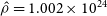
Midplane slices of the density at
 $y = 0$
for each simulation, with increasing jet magnetic field strength from left to right, and the cluster simulation on the far right. All four simulations are plotted at the same total radio source length of 160 kpc. Simulations RAG-B0 and RAG-B16 are plotted at 20 Myr. Simulation RAG-B327 is plotted at 8 Myr. Simulation RAC-B327 is plotted at 17 Myr.
$y = 0$
for each simulation, with increasing jet magnetic field strength from left to right, and the cluster simulation on the far right. All four simulations are plotted at the same total radio source length of 160 kpc. Simulations RAG-B0 and RAG-B16 are plotted at 20 Myr. Simulation RAG-B327 is plotted at 8 Myr. Simulation RAC-B327 is plotted at 17 Myr.
3.2 Dynamics
The dynamics of our jets are highly dependent on the ratio of magnetic to kinetic energy flux in the jet. As described previously by Mukherjee et al. (Reference Mukherjee, Bodo, Mignone, Rossi and Vaidya2020), highly magnetised jets with a toroidal field structure are very narrow and do not follow self-similar evolution. Magnetic field topology influences large-scale jet dynamics (e.g. Koessl, Mueller, & Hillebrandt Reference Koessl, Mueller and Hillebrandt1990; Chen, Heinz, & Hooper Reference Chen, Heinz and Hooper2023), however, the dynamics of our simulations are comparable as the magnetic field is toroidal in all cases.
Figure 1 shows this difference in the morphology of our three simulated jets, plotted at the same total lobe length. The lobes in simulations RAG-B0 and RAG-B16 are almost identical; since the jet magnetic energy is quite low (
 $\ll 1$
% of the total jet power), the magnetic field does not change the dynamics of the jets in simulation RAG-B16 significantly (e.g. Hardcastle & Krause Reference Hardcastle and Krause2014). The lobe in simulation RAG-B327 is narrower by a factor of 2 and reaches the total length of 160 kpc
$\ll 1$
% of the total jet power), the magnetic field does not change the dynamics of the jets in simulation RAG-B16 significantly (e.g. Hardcastle & Krause Reference Hardcastle and Krause2014). The lobe in simulation RAG-B327 is narrower by a factor of 2 and reaches the total length of 160 kpc
 $2.5$
times faster than simulations RAG-B0 and RAG-B16 and
$2.5$
times faster than simulations RAG-B0 and RAG-B16 and
 $2.1$
times faster than simulation RAC-B327. Since simulation RAC-B327 has a denser environment, the expansion of the lobe along the jet axis is inhibited, resulting in a narrow jet head and wide equatorial region of the lobe.
$2.1$
times faster than simulation RAC-B327. Since simulation RAC-B327 has a denser environment, the expansion of the lobe along the jet axis is inhibited, resulting in a narrow jet head and wide equatorial region of the lobe.
Our simulations are comparable to the moderate-powered jets in Mukherjee et al. (Reference Mukherjee, Bodo, Mignone, Rossi and Vaidya2020)’s simulations D (RAG-B16) and F (RAG-B327 and RAC-B327) but shown here on larger scales as they have been evolved for longer. The difference in lobe width and jet stability is the same on these larger scales as that reported by Mukherjee et al. (Reference Mukherjee, Bodo, Mignone, Rossi and Vaidya2020) on galactic scales; the jet in RAG-B16 is disrupted at
 $0.9$
Myr by Kelvin-Helmholtz instabilities, whereas in simulations RAG-B327 and RAC-B327 the jets remain relatively stable to these instabilities due to their higher magnetisation. These simulations confirm the result of Mukherjee et al. (Reference Mukherjee, Bodo, Mignone, Rossi and Vaidya2020) that higher powered, faster jets, with strong magnetic fields are the most stable RMHD jets.
$0.9$
Myr by Kelvin-Helmholtz instabilities, whereas in simulations RAG-B327 and RAC-B327 the jets remain relatively stable to these instabilities due to their higher magnetisation. These simulations confirm the result of Mukherjee et al. (Reference Mukherjee, Bodo, Mignone, Rossi and Vaidya2020) that higher powered, faster jets, with strong magnetic fields are the most stable RMHD jets.
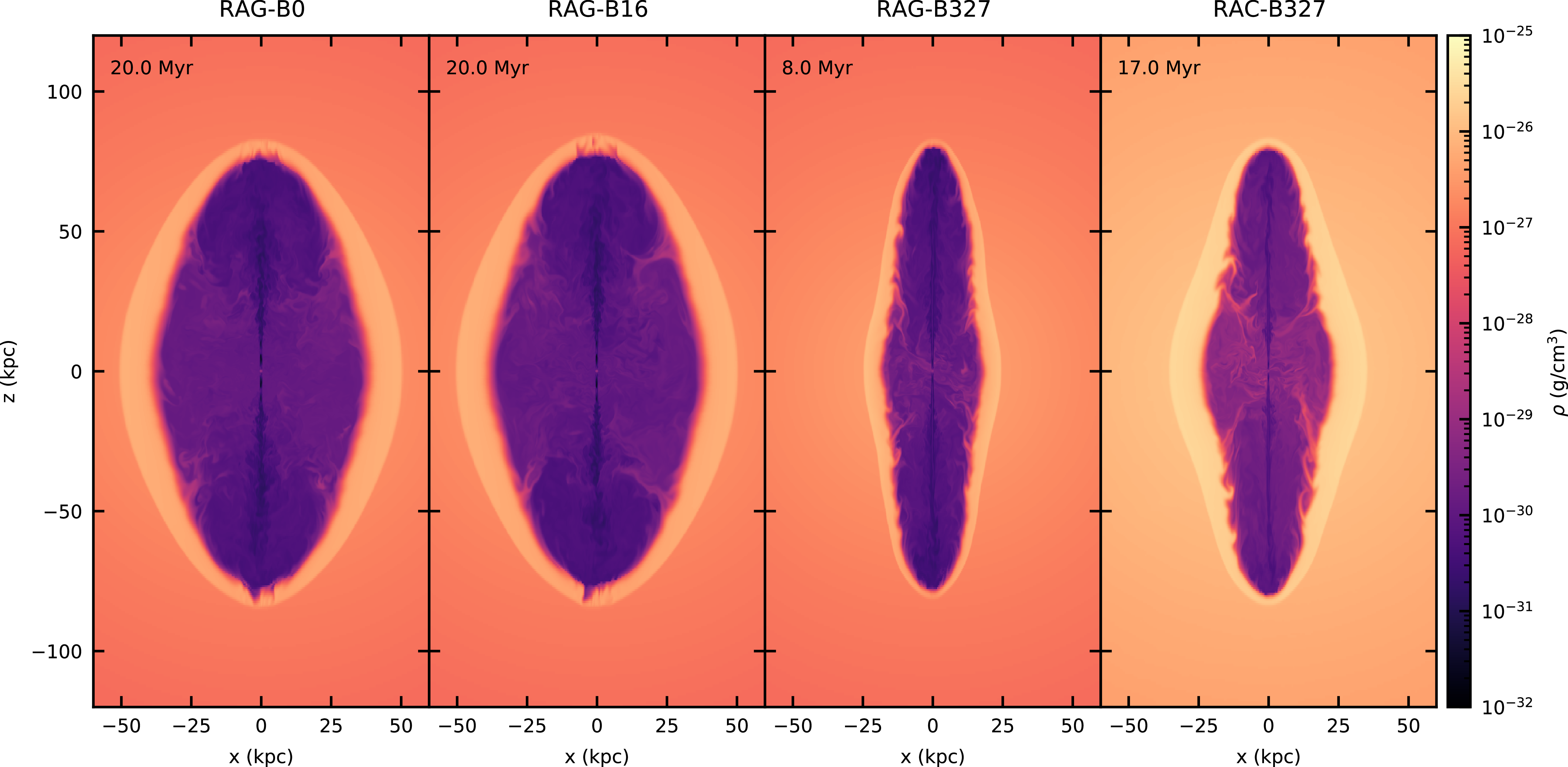
In Figure 2, we plot the pressure in the Lagrangian particles. The jets in simulations RAG-B327 and RAC-B327 terminate in a clear region of enhanced pressure. Simulations RAG-B0 and RAG-B16 are again broadly consistent with one another, with both simulations showing a small region of slightly enhanced pressures at either end of the lobes. However, the particle pressures also show the decollimation of the jet at
 $z \simeq \pm 25$
kpc, shown by the jet particles ‘fanning out’ from the jet axis. This corresponds to the location of jet decollimation due to disruption, after which the jet slows down but keeps expanding outwards.
$z \simeq \pm 25$
kpc, shown by the jet particles ‘fanning out’ from the jet axis. This corresponds to the location of jet decollimation due to disruption, after which the jet slows down but keeps expanding outwards.
Lagrangian particle pressure for each simulation, with increasing jet magnetic field strength from left to right, and the cluster simulation on the far right. The latest particles injected onto the simulation grid are plotted on top. Simulations are plotted at the same times as in Figure 1. Plot insets correspond to the region at
 $z \simeq 25$
kpc where the northern jets in simulations RAG-B0 and RAG-B16 decollimate.
$z \simeq 25$
kpc where the northern jets in simulations RAG-B0 and RAG-B16 decollimate.
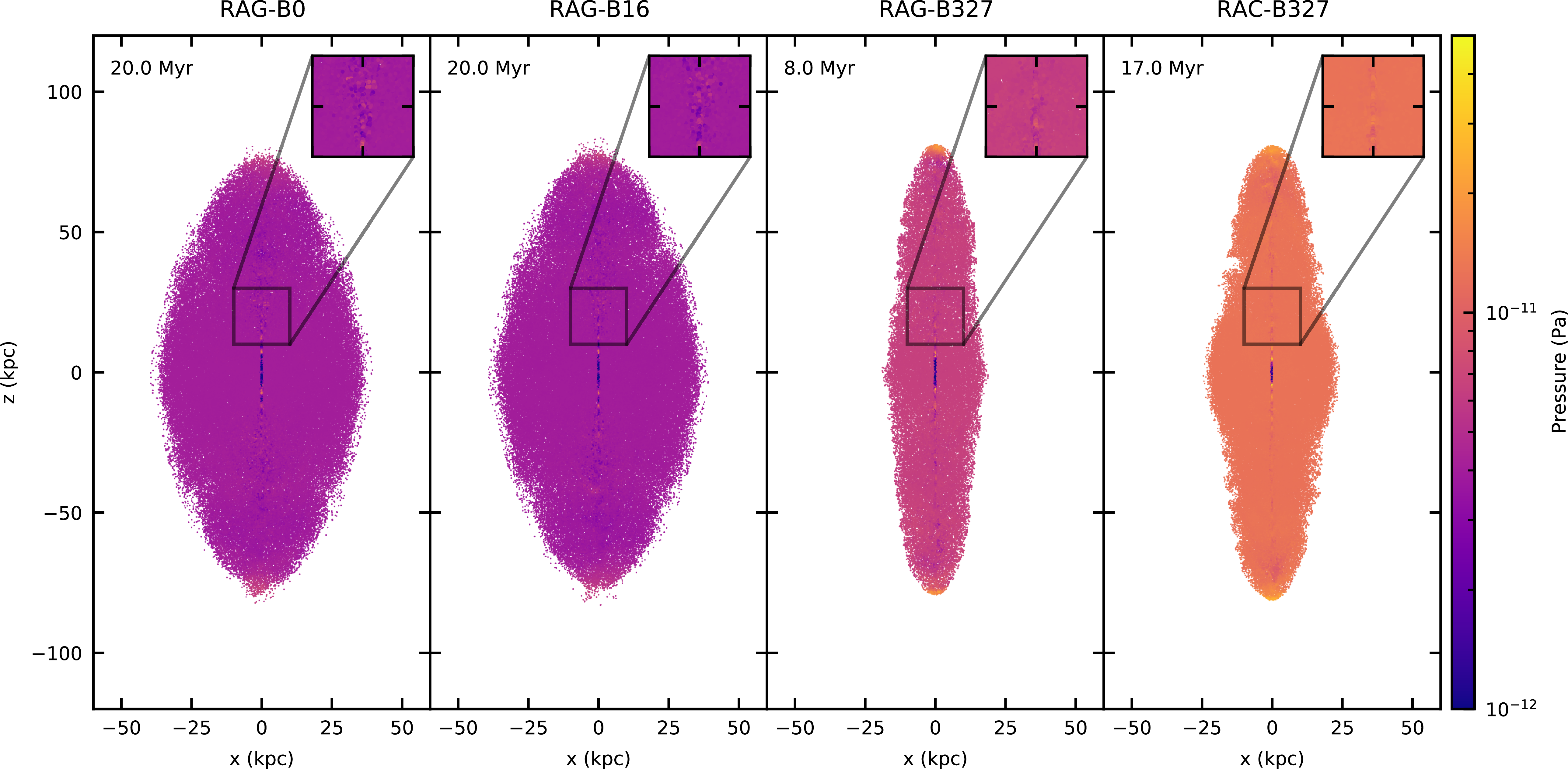
Time since last shock for each Lagrangian particle plotted for each simulation, with increasing jet magnetic field strength from left to right, and the cluster simulation on the far right. The latest particles injected onto the simulation grid are plotted on top. Simulations are plotted at the same times as in Figure 1.
3.2.1 Shock structures
We plot the spatial distribution of the time since each particle was either injected or last shock accelerated (i.e. particle age) in Figure 3, which shows in more detail the differences in jet stability between the three simulations. In simulations RAG-B0 and RAG-B16, we see the particle ages decrease along the jet axis, with the particles fanning out as seen in the spatial distribution of the particle pressures. The shock structures for simulations RAG-B0 and RAG-B16 are most similar to a lobed FR-I-like source.
In comparison, simulations RAG-B327 and RAC-B327 show a clear region of freshly accelerated particles distributed over a working surface with a narrow solid angle at the jet head, which is more typical of a hotspot in an FR-II-like source. We see clear signatures of backflow with an increase in particle age from the hotspot back towards the equatorial plane. At
 $z = \pm 25$
kpc in both these simulations, we see some particles with an increasing age gradient flaring out from the main jet; these ‘flaring points’ correspond to areas of Kelvin-Helmholtz instabilities along the jet. The gradient of particle ages in the backflow is concentrated over a smaller region in simulation RAC-B327 compared to simulation RAG-B327; this is due to the slower propagation of the jet, and hence the slower backflow in the cocoon.
$z = \pm 25$
kpc in both these simulations, we see some particles with an increasing age gradient flaring out from the main jet; these ‘flaring points’ correspond to areas of Kelvin-Helmholtz instabilities along the jet. The gradient of particle ages in the backflow is concentrated over a smaller region in simulation RAC-B327 compared to simulation RAG-B327; this is due to the slower propagation of the jet, and hence the slower backflow in the cocoon.
3.2.2 Magnetic fields
The magnetic field in the jet-inflated cocoon is highly turbulent. Figure 4 shows the spatial distribution of the magnetic field energy density in the particles (weighted by the fluid tracer value as discussed in Section 2.1; this is the relevant magnetic energy for the radiating particles). The locations of strong magnetic fields will correspond to bright emission in synthetic images produced using BRAiSE. Simulation RAG-B16 shows a similar distribution of energy to the pressure; the high magnetic energy density in the jet is fanned out into the lobe, though unlike the pressure, no hotspot is seen. The magnetic energy density is generally higher towards the jet head, and lower towards the equatorial region, though in all regions it varies on small scales, reflecting the turbulent magnetic field seen in the lobe (e.g. Figure 3 of Jerrim et al. Reference Jerrim2024).
Magnetic energy density of the radiating particles for each RMHD simulation, with increasing jet magnetic field strength from left to right, and the cluster simulation on the far right. The latest particles injected onto the simulation grid are plotted on top, however, the general trends on the simulation grid are reproduced. Simulations are plotted at the same times as in Figure 1.

Simulations RAG-B327 and RAC-B327 in general have higher magnetic energy densities in the jet and across the lobe for the same total source length as simulation RAG-B16 due to the higher initial jet magnetic field strength. The edges of the lobe have enhanced magnetic energy density, particularly in locations where we see Kelvin-Helmholtz instabilities in Figure 1. These regions are mixing with the shocked shell of ambient medium, which sweep up the turbulent ambient magnetic field (Jerrim et al. Reference Jerrim2024). Like in simulation RAG-B16, the magnetic energy density is generally higher towards the jet head, and lower towards the equatorial region. Unlike the pressure (Figure 2), there do not seem to be clear regions of enhanced magnetic energy density where the radio hotspots should be in both RAG-B327 and RAC-B327; this is due to kink instabilities disrupting the jet flow just before the jet head.
The differences in environment between the RAG-B327 and RAC-B327 simulations result in a slightly different distribution of high magnetic energy density regions across the cocoon. Since the cluster environment is more dense, the jet head region in simulation RAC-B327 is narrower, creating a bottleneck effect for the particles in the backflow. The particles in the backflow are swept into pockets of the cocoon formed by Kelvin-Helmholtz instabilities at the boundary between the cocoon and the shocked shell of ambient medium surrounding the cocoon. The mixing that these instabilities cause can be seen in Figure 1 (e.g. at
 $x \simeq -10$
,
$x \simeq -10$
,
 $z \simeq 25$
), where these regions cause filaments of the higher density shocked ambient gas to move towards the centre of the cocoon. In addition to slowing down the backflow, this shocked gas also has a high magnetic field due to the compression of the turbulent ambient medium in the shocked shell (e.g. Jerrim et al. Reference Jerrim2024). The particles in these regions will therefore have a slightly higher magnetic energy density than those elsewhere in the cocoon. This non-uniform distribution of magnetic energy is a dynamical effect due to the density of the environment.
$z \simeq 25$
), where these regions cause filaments of the higher density shocked ambient gas to move towards the centre of the cocoon. In addition to slowing down the backflow, this shocked gas also has a high magnetic field due to the compression of the turbulent ambient medium in the shocked shell (e.g. Jerrim et al. Reference Jerrim2024). The particles in these regions will therefore have a slightly higher magnetic energy density than those elsewhere in the cocoon. This non-uniform distribution of magnetic energy is a dynamical effect due to the density of the environment.
The non-magnetic approach to calculating radio emission requires a mapping between pressure and magnetic field strength. We determine an appropriate equipartition factor as defined by the ratio of magnetic to particle energy densities (
 $\eta = \frac{u_B'}{u_e}$
, where
$\eta = \frac{u_B'}{u_e}$
, where
 $u_e$
is defined in Equation (5), and
$u_e$
is defined in Equation (5), and
 $u_B' = u_B / {\rm trc}$
) to describe the average magnetic energy density across the whole lobe for the PRAiSE calculation. Figure 5 shows the evolution of the distribution of the equipartition factor over time in the Lagrangian tracer particles for our RMHD simulations. The distributions for our simulations have peak
$u_B' = u_B / {\rm trc}$
) to describe the average magnetic energy density across the whole lobe for the PRAiSE calculation. Figure 5 shows the evolution of the distribution of the equipartition factor over time in the Lagrangian tracer particles for our RMHD simulations. The distributions for our simulations have peak
 $\eta$
values between
$\eta$
values between
 $0.1$
and
$0.1$
and
 $0.001$
at most times, which is consistent with observations (e.g. Turner, Shabala, & Krause Reference Turner, Shabala and Krause2018b). Because the equipartition factors tend to decrease over time, we adopt the peak in the equipartition factor distribution at each time in our simulations, rather than averaging these peak values over time.
$0.001$
at most times, which is consistent with observations (e.g. Turner, Shabala, & Krause Reference Turner, Shabala and Krause2018b). Because the equipartition factors tend to decrease over time, we adopt the peak in the equipartition factor distribution at each time in our simulations, rather than averaging these peak values over time.
Distributions of the equipartition factor in the Lagrangian particles over time for the RMHD simulations, with increasing jet magnetic field strength from top to bottom, and the cluster simulation shown in the bottom panel. The distributions are shown for every 2 Myr until 20 Myr for each RMHD simulation.
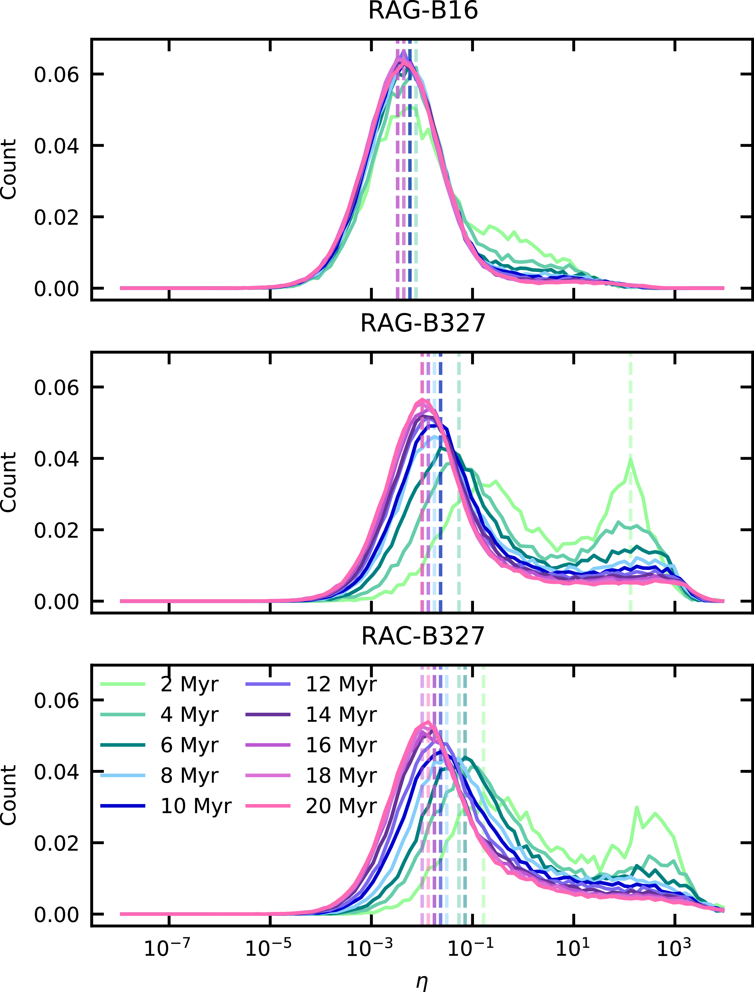
At early times in each simulation, a secondary peak at higher
 $\eta$
values is seen; this is a numerical artefact of how the Lagrangian particles are set with values that are interpolated from the nearest grid cells. For particles at the edges of the lobe, the tracer value is extremely low due to interpolation with grid cells outside the jet, resulting in very high magnetic energy densities, and therefore high
$\eta$
values is seen; this is a numerical artefact of how the Lagrangian particles are set with values that are interpolated from the nearest grid cells. For particles at the edges of the lobe, the tracer value is extremely low due to interpolation with grid cells outside the jet, resulting in very high magnetic energy densities, and therefore high
 $\eta$
values. This effect is more significant in simulation RAG-B327 due to the narrowness of the jet; for the first 2 Myr, we take the secondary peak of the
$\eta$
values. This effect is more significant in simulation RAG-B327 due to the narrowness of the jet; for the first 2 Myr, we take the secondary peak of the
 $\eta$
value distribution to describe the magnetic energy density more accurately within the lobe. These high
$\eta$
value distribution to describe the magnetic energy density more accurately within the lobe. These high
 $\eta$
value particles will not affect the overall synthetic radio emission since their emission will be downweighted by the fluid tracer value.
$\eta$
value particles will not affect the overall synthetic radio emission since their emission will be downweighted by the fluid tracer value.
3.3 Surface brightness
As described in Section 2, we generate synthetic radio synchrotron emission including IC and adiabatic losses using either the particle pressures (PRAiSE) or the particle magnetic field strengths (BRAiSE). Following Yates-Jones et al. (Reference Yates-Jones, Turner, Shabala and Krause2022), we define the spectral index as
 $S_\nu \propto \nu^{-\alpha}$
and use an injection index of
$S_\nu \propto \nu^{-\alpha}$
and use an injection index of
 $\alpha_{\rm inj} = 0.6$
, and minimum and maximum Lorentz factors
$\alpha_{\rm inj} = 0.6$
, and minimum and maximum Lorentz factors
 $\gamma_{\rm min} = 500$
and
$\gamma_{\rm min} = 500$
and
 $\gamma_{\rm max} = 10^5$
, respectively.
$\gamma_{\rm max} = 10^5$
, respectively.
We calculate the surface brightness images in the plane of the sky following the method outlined in Yates-Jones et al. (Reference Yates-Jones, Turner, Shabala and Krause2022). The images have been convolved with a 2D Gaussian beam with FWHM of
 $2.97''$
at a redshift of
$2.97''$
at a redshift of
 $z = 0.05$
and
$z = 0.05$
and
 $0.35''$
at
$0.35''$
at
 $z = 2$
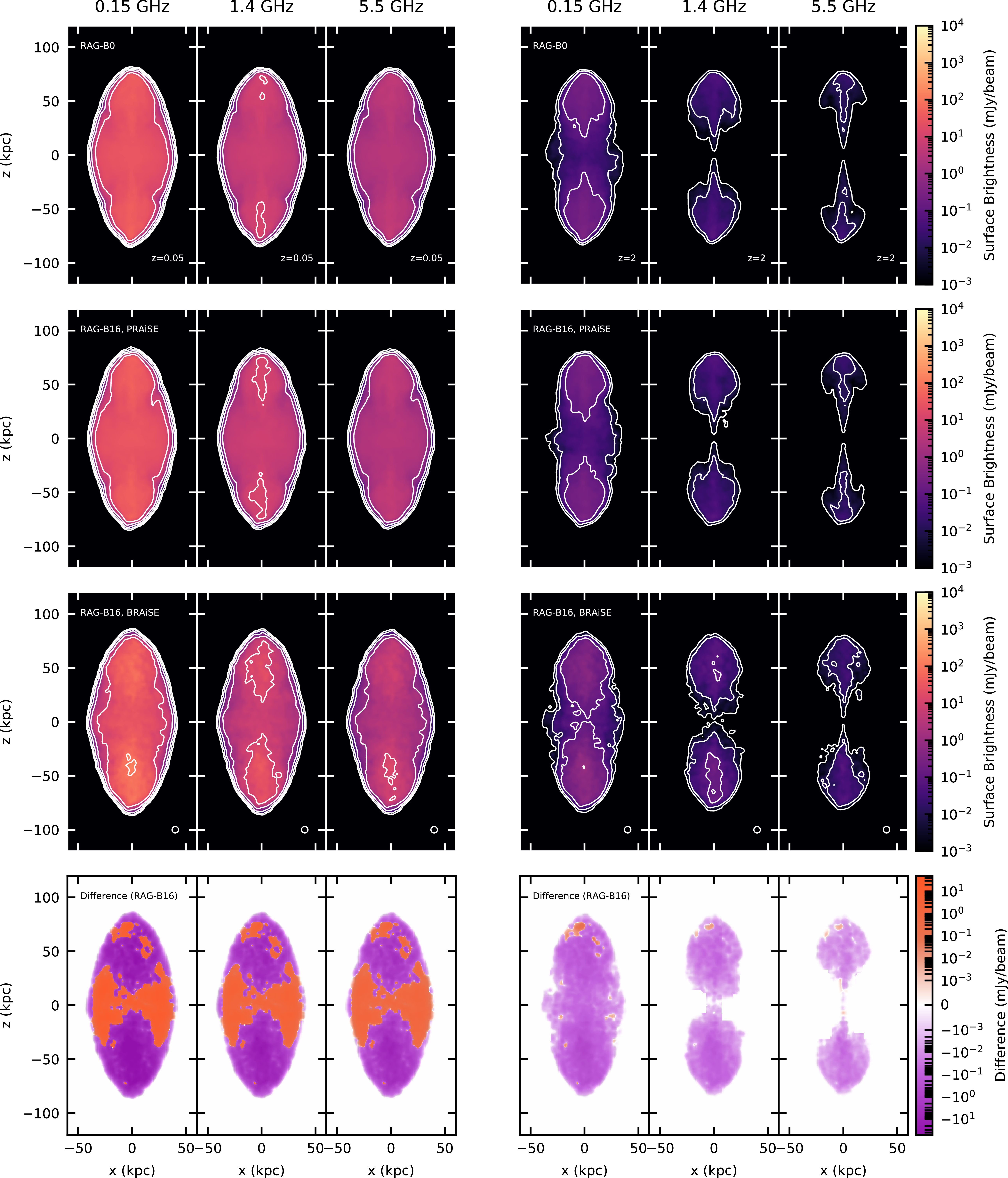
(this corresponds to the same physical beam size of 3 kpc). The choice of this beam FWHM is representative of high-resolution SKA pathfinder instruments (Morabito et al. Reference Morabito2022). In Figure 6, we show the surface brightness images for simulations RAG-B0 and RAG-B16 at 20 Myr; for the latter RMHD simulation, we include both PRAiSE and BRAiSE images and the difference between them. In Figure 7 we plot the surface brightness images and their difference map for simulation RAG-B327 at 8 Myr, and similarly plot these images at 17 Myr for simulation RAC-B327 in Figure 8.
$z = 2$
(this corresponds to the same physical beam size of 3 kpc). The choice of this beam FWHM is representative of high-resolution SKA pathfinder instruments (Morabito et al. Reference Morabito2022). In Figure 6, we show the surface brightness images for simulations RAG-B0 and RAG-B16 at 20 Myr; for the latter RMHD simulation, we include both PRAiSE and BRAiSE images and the difference between them. In Figure 7 we plot the surface brightness images and their difference map for simulation RAG-B327 at 8 Myr, and similarly plot these images at 17 Myr for simulation RAC-B327 in Figure 8.
PRAiSE and BRAiSE surface brightnesses (Stokes I) for the RAG-B0 and RAG-B16 simulations at 20 Myr. Contours are
 $0.001, 0.01, 0.1, 1, 10, 100, 1\,000,$
and
$0.001, 0.01, 0.1, 1, 10, 100, 1\,000,$
and
 $10\,000$
mJy/beam. Each surface brightness is plotted for two redshifts (
$10\,000$
mJy/beam. Each surface brightness is plotted for two redshifts (
 $z = 0.05, 2$
, as indicated in the bottom right-hand corner of the top row) and three frequencies (
$z = 0.05, 2$
, as indicated in the bottom right-hand corner of the top row) and three frequencies (
 $0.15, 1.4,$
and
$0.15, 1.4,$
and
 $5.5$
GHz). The bottom row corresponds to the difference between the PRAiSE and BRAiSE surface brightnesses for simulation RAG-B16. The telescope observing beam is shown as a circle in the bottom right-hand corner of the panels in the BRAiSE surface brightness row.
$5.5$
GHz). The bottom row corresponds to the difference between the PRAiSE and BRAiSE surface brightnesses for simulation RAG-B16. The telescope observing beam is shown as a circle in the bottom right-hand corner of the panels in the BRAiSE surface brightness row.
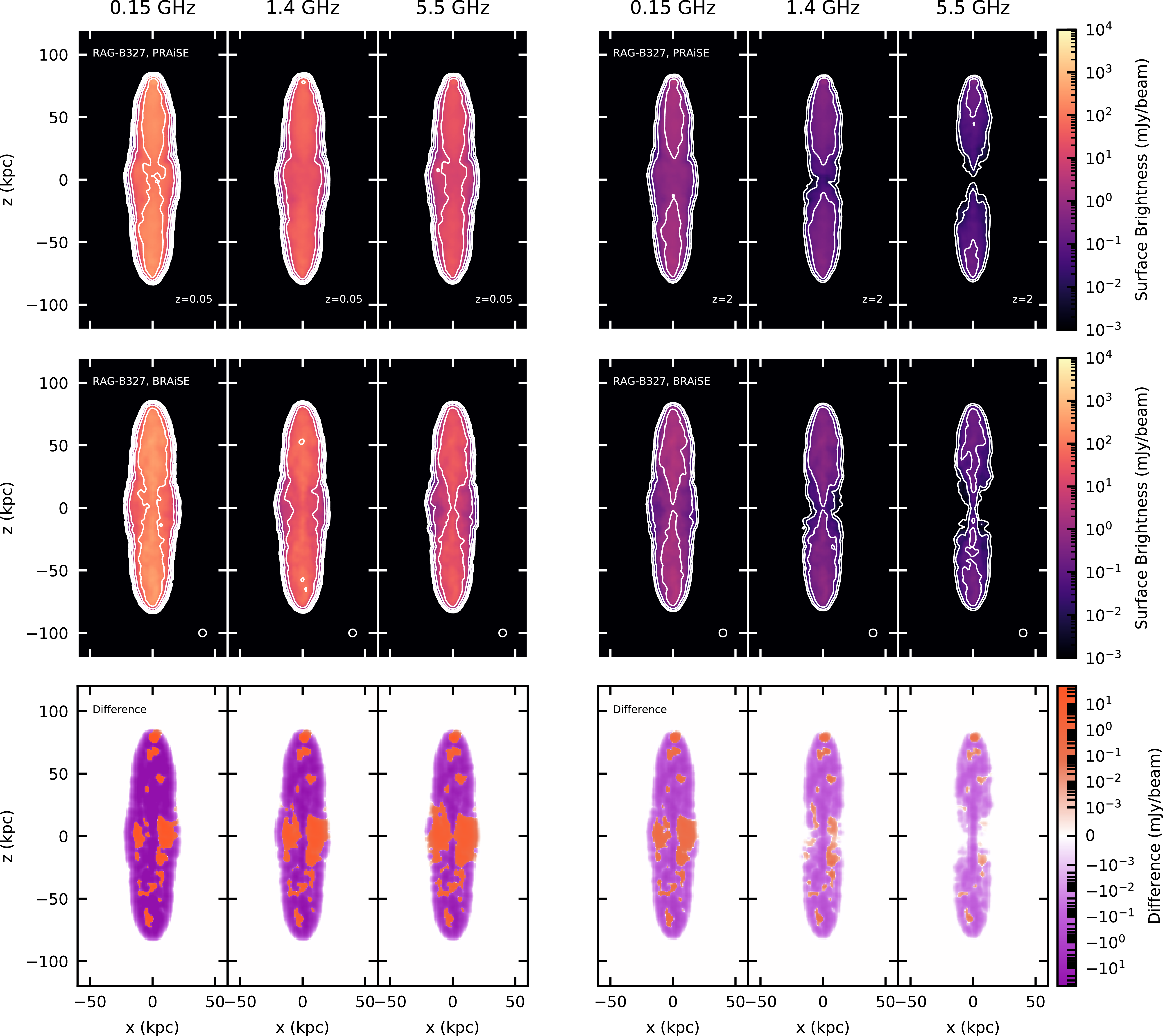
PRAiSE and BRAiSE surface brightnesses (Stokes’ I) for the RAG-B327 simulation at 8 Myr. Contours, redshifts, frequencies, and observing beam are as for Figure 6. The bottom row corresponds to the difference between the PRAiSE and BRAiSE surface brightnesses for simulation RAG-B327.
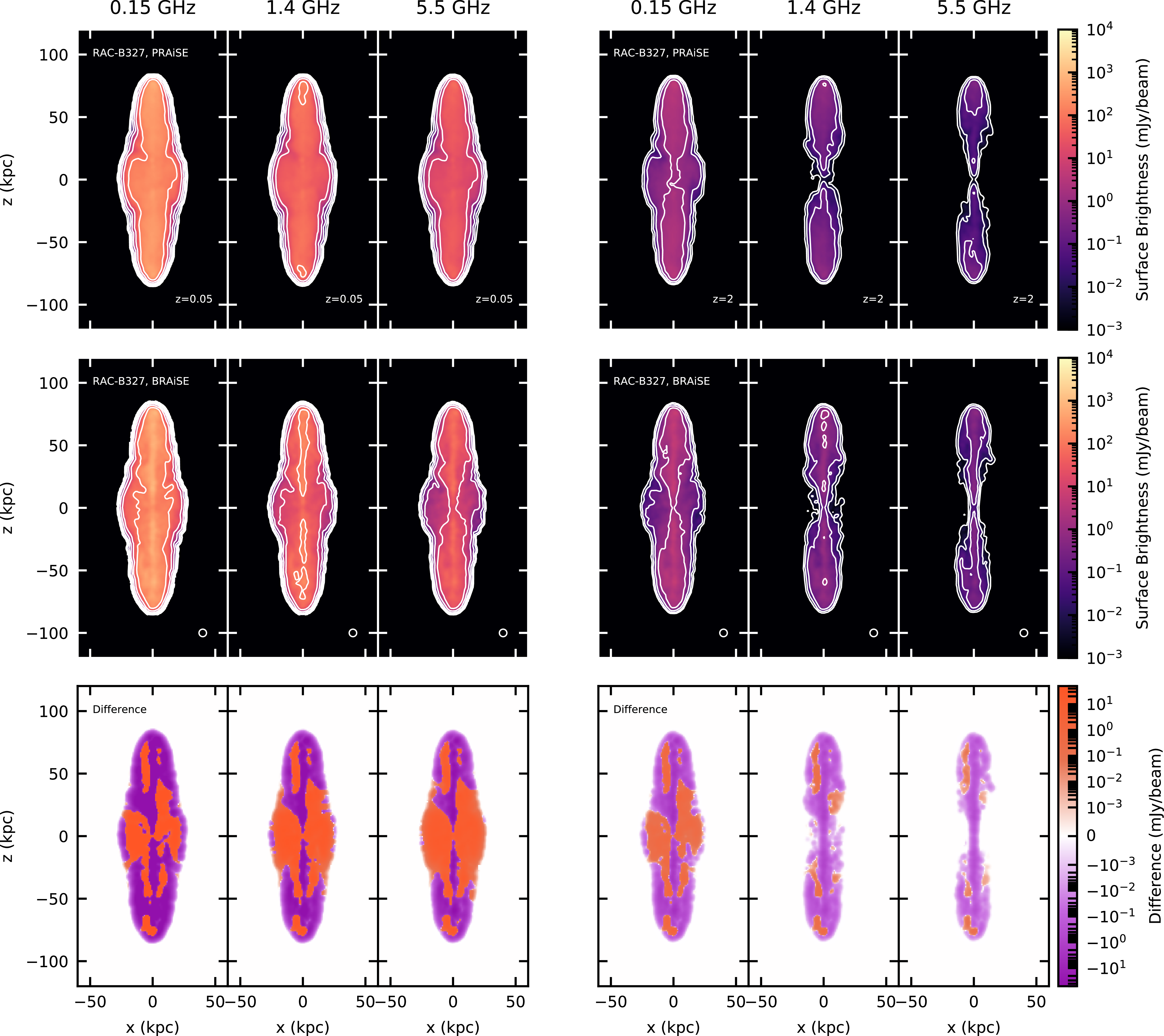
PRAiSE and BRAiSE surface brightnesses (Stokes’ I) for the RAC-B327 simulation at 17 Myr. Contours, redshifts, frequencies, and observing beam are as for Figure 6. The bottom row corresponds to the difference between the PRAiSE and BRAiSE surface brightnesses for simulation RAC-B327.
For simulations RAG-B0 and RAG-B16, we see minor differences between the PRAiSE surface brightness images. The morphology is broadly consistent between the two simulations, as expected given the similarity between the dynamical properties of these simulations. This confirms that when the jet magnetic field is subdominant, the radio emission using PRAiSE is broadly consistent with the radio emission from an RHD simulation. We see clearer small-scale structure in the BRAiSE surface brightness image due to the turbulent magnetic field structure seen in Figure 4 (as also seen in Tregillis et al. Reference Tregillis, Jones and Ryu2004; Huarte-Espinosa et al. Reference Huarte-Espinosa, Krause and Alexander2011a; Hardcastle & Krause Reference Hardcastle and Krause2014). The difference map shows that in general, BRAiSE is brighter along the jet and in the main lobe region, but PRAiSE is brighter in the equatorial region. This is due to the distribution of magnetic fields: in PRAiSE the effective lobe magnetic field is dependent on the pressure, which is relatively constant across the lobe (Figure 2) compared to the turbulent magnetic field (Figure 4). As a result, the emission along the jet will be underpredicted and the emission in the equatorial regions will be overpredicted. The relative difference in emission is consistent across all frequencies at low redshift (
 $z = 0.05$
).
$z = 0.05$
).
For the higher jet magnetic field simulations, we again find more defined small-scale structure in the BRAiSE surface brightness image. The BRAiSE surface brightness also shows a defined cone of bright emission which is not seen in the PRAiSE image at
 $z \pm 25$
kpc (outlined by the highest contour at
$z \pm 25$
kpc (outlined by the highest contour at
 $5.5$
GHz). This is due to the presence of particles with high magnetic energies in the flaring region (as discussed in Section 3.2.1). This region is highly affected by Kelvin-Helmholtz instabilities that allow some of the radiating particles to escape the jet channel and flow forward into the lobe. This effect is stronger in simulation RAG-B327 than simulation RAC-B327, as the confinement of the cluster environment aids the stability of the jet in the latter simulation. This flaring region plus hotspot emission results in a bimodal surface brightness morphology that resembles hybrid sources such as J1154+513, J1206+503, and J1313+507 (Harwood, Vernstrom, & Stroe Reference Harwood, Vernstrom and Stroe2020).
$5.5$
GHz). This is due to the presence of particles with high magnetic energies in the flaring region (as discussed in Section 3.2.1). This region is highly affected by Kelvin-Helmholtz instabilities that allow some of the radiating particles to escape the jet channel and flow forward into the lobe. This effect is stronger in simulation RAG-B327 than simulation RAC-B327, as the confinement of the cluster environment aids the stability of the jet in the latter simulation. This flaring region plus hotspot emission results in a bimodal surface brightness morphology that resembles hybrid sources such as J1154+513, J1206+503, and J1313+507 (Harwood, Vernstrom, & Stroe Reference Harwood, Vernstrom and Stroe2020).
For simulations RAG-B327 and RAC-B327, the jet emission using BRAiSE is brighter than in PRAiSE due to the high jet magnetic field strength which is not captured in the peak equipartition factor used in PRAiSE. Despite this enhanced jet emission, the difference map clearly shows that BRAiSE lacks defined hotspots in simulation RAG-B327. This is partially due to the kink instabilities in the jet spreading the magnetic energy (as noted in Section 3.2.2), similar to what Tingay et al. (Reference Tingay, Lenc, Brunetti and Bondi2008) hypothesise is occurring in the southeast hotspot of Pictor A. This results in a larger working surface for the jet head; however, since the pressure is still enhanced in this region, we still find a hotspot-like structure when using PRAiSE. This enhanced jet emission is discussed further in Section 3.4.
For simulations RAG-B327 and RAC-B327, PRAiSE has some brighter areas in the equatorial regions of the lobe that coincide with locations of lower magnetic energy density (Figure 4). There are also significant differences between PRAiSE and BRAiSE in the small-scale structure for simulation RAC-B327. This is due to the distribution of magnetic energy density in the lobe (as discussed in Section 3.2.2); BRAiSE shows brighter regions of surface brightness in the areas where the backflow of particles from the hotspot has been slowed down due to the mixing of the cocoon with the shocked shell. An example of this bright region is at
 $x \simeq -10$
,
$x \simeq -10$
,
 $z \simeq 25$
, corresponding to a region of significant mixing. The restricted movement of the backflow into the cocoon due to the higher density environment can be seen at high redshift (
$z \simeq 25$
, corresponding to a region of significant mixing. The restricted movement of the backflow into the cocoon due to the higher density environment can be seen at high redshift (
 $z = 2$
) for PRAiSE.
$z = 2$
) for PRAiSE.
In all simulations, we find that the differences between PRAiSE and BRAiSE are consistent at a higher redshift (
 $z = 2$
); the BRAiSE surface brightness is in general higher, meaning that more of the radio lobe is visible at higher redshifts (and frequencies). Therefore, PRAiSE produces surface brightnesses that are more susceptible to IC losses. These losses result in more ‘pinched’ or narrower lobes for all simulations, which become more extreme at higher frequencies. In simulation RAG-B327, this effect is more subtle due to the narrowness of the lobe and brightness of the jet. At a redshift of
$z = 2$
); the BRAiSE surface brightness is in general higher, meaning that more of the radio lobe is visible at higher redshifts (and frequencies). Therefore, PRAiSE produces surface brightnesses that are more susceptible to IC losses. These losses result in more ‘pinched’ or narrower lobes for all simulations, which become more extreme at higher frequencies. In simulation RAG-B327, this effect is more subtle due to the narrowness of the lobe and brightness of the jet. At a redshift of
 $z = 2$
, the difference maps show smaller contrasts due to the reduced magnitude of the synchrotron emission and greater importance of IC losses, which are the same for both PRAiSE and BRAiSE.
$z = 2$
, the difference maps show smaller contrasts due to the reduced magnitude of the synchrotron emission and greater importance of IC losses, which are the same for both PRAiSE and BRAiSE.
The integrated
 $0.15$
GHz luminosity at a redshift of
$0.15$
GHz luminosity at a redshift of
 $z = 0.05$
for all four simulations are not similar to one another (Table 2), due the clear differences in pressure and lobe magnetic field strength at the same total lobe length. BRAiSE has higher luminosities than PRAiSE (
$z = 0.05$
for all four simulations are not similar to one another (Table 2), due the clear differences in pressure and lobe magnetic field strength at the same total lobe length. BRAiSE has higher luminosities than PRAiSE (
 $1.8\times$
for RAG-B16,
$1.8\times$
for RAG-B16,
 $1.4\times$
for RAG-B327 and
$1.4\times$
for RAG-B327 and
 $1.3\times$
for RAC-B327) due to the higher magnetic energy densities used, rather than the constant equipartition factor (as discussed earlier). Simulation RAC-B327 has higher luminosities due to the increased environment density confining the jet (Shabala & Godfrey Reference Shabala and Godfrey2013).
$1.3\times$
for RAC-B327) due to the higher magnetic energy densities used, rather than the constant equipartition factor (as discussed earlier). Simulation RAC-B327 has higher luminosities due to the increased environment density confining the jet (Shabala & Godfrey Reference Shabala and Godfrey2013).
Summary of the total 0.15 GHz luminosity for each of our simulations and method of calculating the radio emission. The right-most column shows the ratio of each luminosity to the luminosity of RAG-B0 using PRAiSE.
3.4 Radio morphology
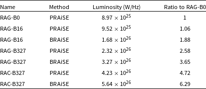
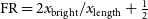
The FR morphological classifications of our radio sources are not clearly defined. We plot the FR index over time in Figure 9, following the method outlined in Krause et al. (Reference Krause, Alexander, Riley and Hopton2012). The FR index is defined as
 ${\rm FR} = 2 x_{\rm bright}/x_{\rm length} + \frac{1}{2}$
, where
${\rm FR} = 2 x_{\rm bright}/x_{\rm length} + \frac{1}{2}$
, where
 $x_{\rm bright}$
is the length from the origin to the brightest pixel in the surface brightness image, and
$x_{\rm bright}$
is the length from the origin to the brightest pixel in the surface brightness image, and
 $x_{\rm length}$
is the length from the origin to the furthest pixel that has a surface brightness within 2 dex of the brightest pixel. Consistent with Yates-Jones et al. (Reference Yates-Jones, Turner, Shabala and Krause2022), we calculate the FR index at
$x_{\rm length}$
is the length from the origin to the furthest pixel that has a surface brightness within 2 dex of the brightest pixel. Consistent with Yates-Jones et al. (Reference Yates-Jones, Turner, Shabala and Krause2022), we calculate the FR index at
 $0.15$
GHz. The dividing line shown on the plot between the FR-I and FR-II classes is at
$0.15$
GHz. The dividing line shown on the plot between the FR-I and FR-II classes is at
 $1.5$
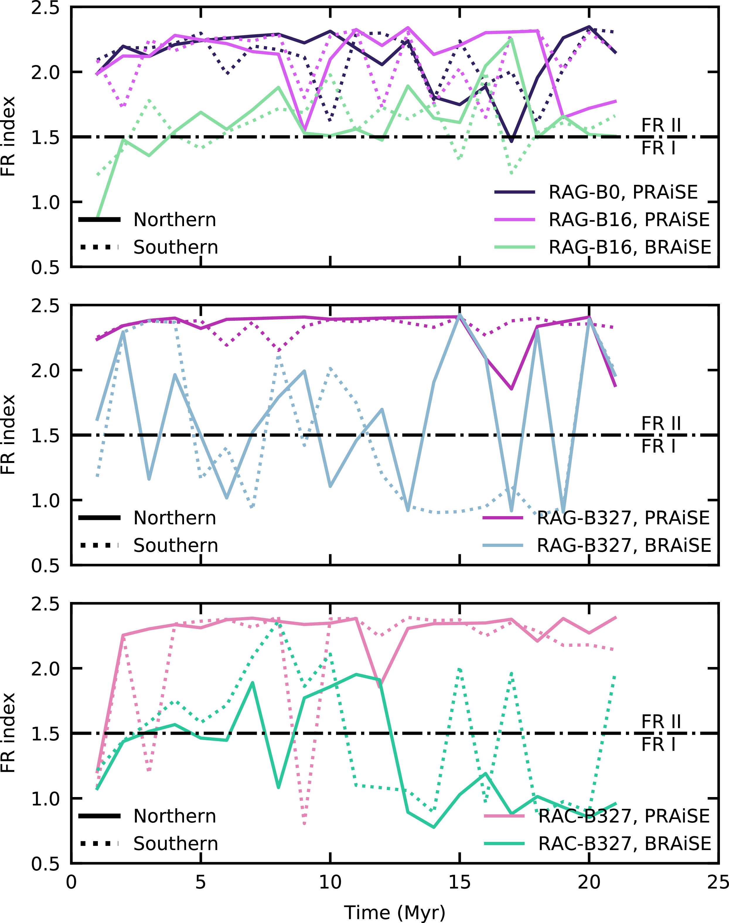
; any source with an FR index below this threshold is classed as an FR-I, and a source above the threshold is classed as an FR-II. Figure 10 demonstrates the peak surface brightness as a function of location along the jet axis at 20 Myr for simulation RAG-B16, 8 Myr for simulation RAG-B327, and 17 Myr for simulation RAC-B327.
$1.5$
; any source with an FR index below this threshold is classed as an FR-I, and a source above the threshold is classed as an FR-II. Figure 10 demonstrates the peak surface brightness as a function of location along the jet axis at 20 Myr for simulation RAG-B16, 8 Myr for simulation RAG-B327, and 17 Myr for simulation RAC-B327.
FR indices at
 $0.15$
GHz and
$0.15$
GHz and
 $z = 0.05$
over time for each simulation and emission code shown in Figures 6 (top panel), 7 (middle panel) and 8 (bottom panel). The classification dividing line is shown with a dot-dashed line at
$z = 0.05$
over time for each simulation and emission code shown in Figures 6 (top panel), 7 (middle panel) and 8 (bottom panel). The classification dividing line is shown with a dot-dashed line at
 $FR = 1.5$
. Solid lines correspond to the northern (upper) jet, and dotted lines correspond to the southern (lower) jet.
$FR = 1.5$
. Solid lines correspond to the northern (upper) jet, and dotted lines correspond to the southern (lower) jet.

We find for each simulation that BRAiSE produces a surface brightness image that has a lower FR index at most times in comparison to PRAiSE. The PRAiSE results for simulations RAG-B0 and RAG-B16 are broadly consistent with one another, with a time-averaged FR index across both lobes of
 $2.1$
. However, the BRAiSE result for simulation RAG-B16 has a time-averaged FR index across both lobes of
$2.1$
. However, the BRAiSE result for simulation RAG-B16 has a time-averaged FR index across both lobes of
 $1.6$
. This is due to the brighter emission along the jet axis in BRAiSE corresponding to the regions of high magnetic energy density (Figure 4). In Figure 10, we see that at 20 Myr, the BRAiSE emission in both jets is brightest at approximately 52% of the total jet length, unlike for the southern jet in PRAiSE, which is brightest at 90% of the total jet length. This difference in location of the bright emission leads to the lower value of the FR index. As discussed in Section 3.2.1, this source is a lobed FR-I-like source, rather than a true FR-II. The FR indices found using the BRAiSE emission code are most consistent with this morphological classification.
$1.6$
. This is due to the brighter emission along the jet axis in BRAiSE corresponding to the regions of high magnetic energy density (Figure 4). In Figure 10, we see that at 20 Myr, the BRAiSE emission in both jets is brightest at approximately 52% of the total jet length, unlike for the southern jet in PRAiSE, which is brightest at 90% of the total jet length. This difference in location of the bright emission leads to the lower value of the FR index. As discussed in Section 3.2.1, this source is a lobed FR-I-like source, rather than a true FR-II. The FR indices found using the BRAiSE emission code are most consistent with this morphological classification.
The FR indices in simulation RAG-B327 are quite different for the two emission codes. The time-averaged FR index for both lobes is
 $2.3$
in PRAiSE, whereas it is
$2.3$
in PRAiSE, whereas it is
 $1.6$
in BRAiSE. In the difference maps shown in Figure 7, we see clearly that the hotspots are brighter in PRAiSE. This is due to the increase in pressure at the end of the lobe; the magnetic energy is not significantly increased in this region (Figure 4). At the time shown in Figure 10 (8 Myr), the jets in simulation RAG-B327 are disrupted and the magnetic energy is distributed over a wider solid angle, which increases this difference in surface brightness in the hotspot region (particularly for the northern jet). It is interesting to note that there is a lack of clear classification at this time, and even as the source continues to evolve.
$1.6$
in BRAiSE. In the difference maps shown in Figure 7, we see clearly that the hotspots are brighter in PRAiSE. This is due to the increase in pressure at the end of the lobe; the magnetic energy is not significantly increased in this region (Figure 4). At the time shown in Figure 10 (8 Myr), the jets in simulation RAG-B327 are disrupted and the magnetic energy is distributed over a wider solid angle, which increases this difference in surface brightness in the hotspot region (particularly for the northern jet). It is interesting to note that there is a lack of clear classification at this time, and even as the source continues to evolve.
Simulation RAC-B327 shows very similar FR indices to simulation RAG-B327 for both PRAiSE and BRAiSE; the time-averaged FR index for both lobes is
 $2.2$
in PRAiSE and
$2.2$
in PRAiSE and
 $1.4$
for BRAiSE. The jet emission is quite prominent in this simulation; Figure 10 shows strong emission at
$1.4$
for BRAiSE. The jet emission is quite prominent in this simulation; Figure 10 shows strong emission at
 $z \simeq \pm 25$
kpc, coincident with the flaring region, but also strong emission at the hotspot of the northern jet (
$z \simeq \pm 25$
kpc, coincident with the flaring region, but also strong emission at the hotspot of the northern jet (
 $z \simeq 75$
kpc). On average, the flaring region is brighter than the hotspots, leading to the FR-I classification. The low (
$z \simeq 75$
kpc). On average, the flaring region is brighter than the hotspots, leading to the FR-I classification. The low (
 $\lt 1.5$
) FR indices for PRAiSE at early times are due to rapid changes in direction of jet propagation, which in turn change the working surface of the jet and therefore the enhancement of the pressure in the hotspot region. This change in direction is caused by the interaction of the jet with its environment; the turbulent ambient magnetic field introduces inhomogeneities that alter the propagation of the jet.
$\lt 1.5$
) FR indices for PRAiSE at early times are due to rapid changes in direction of jet propagation, which in turn change the working surface of the jet and therefore the enhancement of the pressure in the hotspot region. This change in direction is caused by the interaction of the jet with its environment; the turbulent ambient magnetic field introduces inhomogeneities that alter the propagation of the jet.
Depending on the magnetisation of the jet and the interaction with its environment, the difference in the emission calculation method can lead to different FR classifications of the same source. The radio and dynamical classifications are inconsistent since the lobed FR-I-like sources (as identified by their shock structures) in simulations RAG-B0 and RAG-B16 produce FR-II-like radio emission (as identified by their FR indices, for both emission code methods). When using BRAiSE to include the magnetic field in the calculation of synchrotron emission, the broad morphological features of the lobes are consistent with the PRAiSE result. The emission in the jet and its associated flaring region is underpredicted for both low and high magnetisation jets in PRAiSE; this also leads to a lower overall luminosity. For high magnetisation jets, the hotspot emission is overpredicted by PRAiSE at most times, but this depends on the interaction of the jet with its environment. By including the magnetic field in the radio synchrotron emission calculation, we can also reveal details of the jet-environment interaction (e.g. simulation RAC-B327).
To ensure that these results are not an artefact of calculating the surface brightness using the Lagrangian particles, we have assessed the convergence of the calculated emissivity for different numbers of particles injected onto the simulation grid over time. We find that our particle injection rate of 80 particles per
 $0.01$
Myr is more than sufficient to recover the total lobe emissivity, which is constant for an injection rate above 20 particles per
$0.01$
Myr is more than sufficient to recover the total lobe emissivity, which is constant for an injection rate above 20 particles per
 $0.01$
Myr. The flux density of the fast jet slowly decreases as more particles are added, however, this contributes a small fraction of the total emission. We note that local brightness inhomogeneities in the surface brightness images are smoothed out somewhat as the number of particles increase, and we caution against over-interpreting detailed structure in the surface brightness.
$0.01$
Myr. The flux density of the fast jet slowly decreases as more particles are added, however, this contributes a small fraction of the total emission. We note that local brightness inhomogeneities in the surface brightness images are smoothed out somewhat as the number of particles increase, and we caution against over-interpreting detailed structure in the surface brightness.
4. Polarisation
4.1 Fractional polarisation without Faraday rotation
The differences in jet dynamics due to jet magnetisation impact the polarisation properties of our simulated sources. In Figure 11 we plot the fractional polarisation overlaid with contours corresponding to the Stokes I emission (from Figures 6, 7, 8) for each of our RMHD simulations. The length of the vectors corresponds to the fractional polarisation and the direction indicates the inferred ‘magnetic field direction’,
 $\chi_B = \frac{1}{2} \arctan{U/Q} + \frac{\pi}{2}$
, following Hardcastle & Krause (Reference Hardcastle and Krause2014). Two frequencies are plotted (
$\chi_B = \frac{1}{2} \arctan{U/Q} + \frac{\pi}{2}$
, following Hardcastle & Krause (Reference Hardcastle and Krause2014). Two frequencies are plotted (
 $0.15$
and
$0.15$
and
 $1.4$
GHz), at low resolution (beam FWHM of 9 kpc, corresponding to
$1.4$
GHz), at low resolution (beam FWHM of 9 kpc, corresponding to
 $8.91''$
at
$8.91''$
at
 $z = 0.05$
and
$z = 0.05$
and
 $1.05''$
at
$1.05''$
at
 $z = 2$
) and high resolution (beam FWHM of 3 kpc, corresponding to
$z = 2$
) and high resolution (beam FWHM of 3 kpc, corresponding to
 $2.97''$
at
$2.97''$
at
 $z = 0.05$
and
$z = 0.05$
and
 $0.35''$
at
$0.35''$
at
 $z = 2$
) in the left- and right-hand columns for each frequency, respectively. The low resolution beam FWHM is consistent with beam FWHMs in current and upcoming polarisation surveys, which typically range between
$z = 2$
) in the left- and right-hand columns for each frequency, respectively. The low resolution beam FWHM is consistent with beam FWHMs in current and upcoming polarisation surveys, which typically range between
 $1 - 15''$
(see Table 3 of Jerrim et al. Reference Jerrim2024). For each frequency and resolution, we plot low (
$1 - 15''$
(see Table 3 of Jerrim et al. Reference Jerrim2024). For each frequency and resolution, we plot low (
 $z = 0.05$
) and high (
$z = 0.05$
) and high (
 $z = 2$
) redshift images in the first four and latter four columns, respectively. We have held the physical pixel and beam sizes constant across redshifts to compare the effect of IC losses on the fractional polarisation. In the upper three rows, we plot the raw fractional polarisation images, and in the lower three rows, we plot the depolarised by Faraday rotation fractional polarisation images (discussed in Section 4.2 below).
$z = 2$
) redshift images in the first four and latter four columns, respectively. We have held the physical pixel and beam sizes constant across redshifts to compare the effect of IC losses on the fractional polarisation. In the upper three rows, we plot the raw fractional polarisation images, and in the lower three rows, we plot the depolarised by Faraday rotation fractional polarisation images (discussed in Section 4.2 below).
Fractional polarisation maps for the RMHD simulations using BRAiSE. The length of the vectors corresponds to the magnitude of the fractional polarisation at each location and the direction of the vectors indicates the ‘magnetic field direction’. Each fractional polarisation map is plotted for two redshifts (
 $z = 0.05, 2$
, for the left- and right-hand groups, respectively) and two resolutions (beam FWHM
$z = 0.05, 2$
, for the left- and right-hand groups, respectively) and two resolutions (beam FWHM
 $= 3, 9$
kpc, shown as circles in the bottom right-hand corner in the middle row). The upper and lower groups correspond to the raw polarisation images and the depolarised images, respectively. For the depolarised images of RAC-B327 at
$= 3, 9$
kpc, shown as circles in the bottom right-hand corner in the middle row). The upper and lower groups correspond to the raw polarisation images and the depolarised images, respectively. For the depolarised images of RAC-B327 at
 $z = 0.05$
and
$z = 0.05$
and
 $0.15$
GHz, the circles centrered at
$0.15$
GHz, the circles centrered at
 $x = -20$
,
$x = -20$
,
 $z = 25$
correspond to the location discussed in Section 4.2. Contours at
$z = 25$
correspond to the location discussed in Section 4.2. Contours at
 $z = 0.05$
are at 10 and 100 mJy/beam, and contours at
$z = 0.05$
are at 10 and 100 mJy/beam, and contours at
 $z = 2$
are at
$z = 2$
are at
 $0.1$
and 1 mJy/beam.
$0.1$
and 1 mJy/beam.
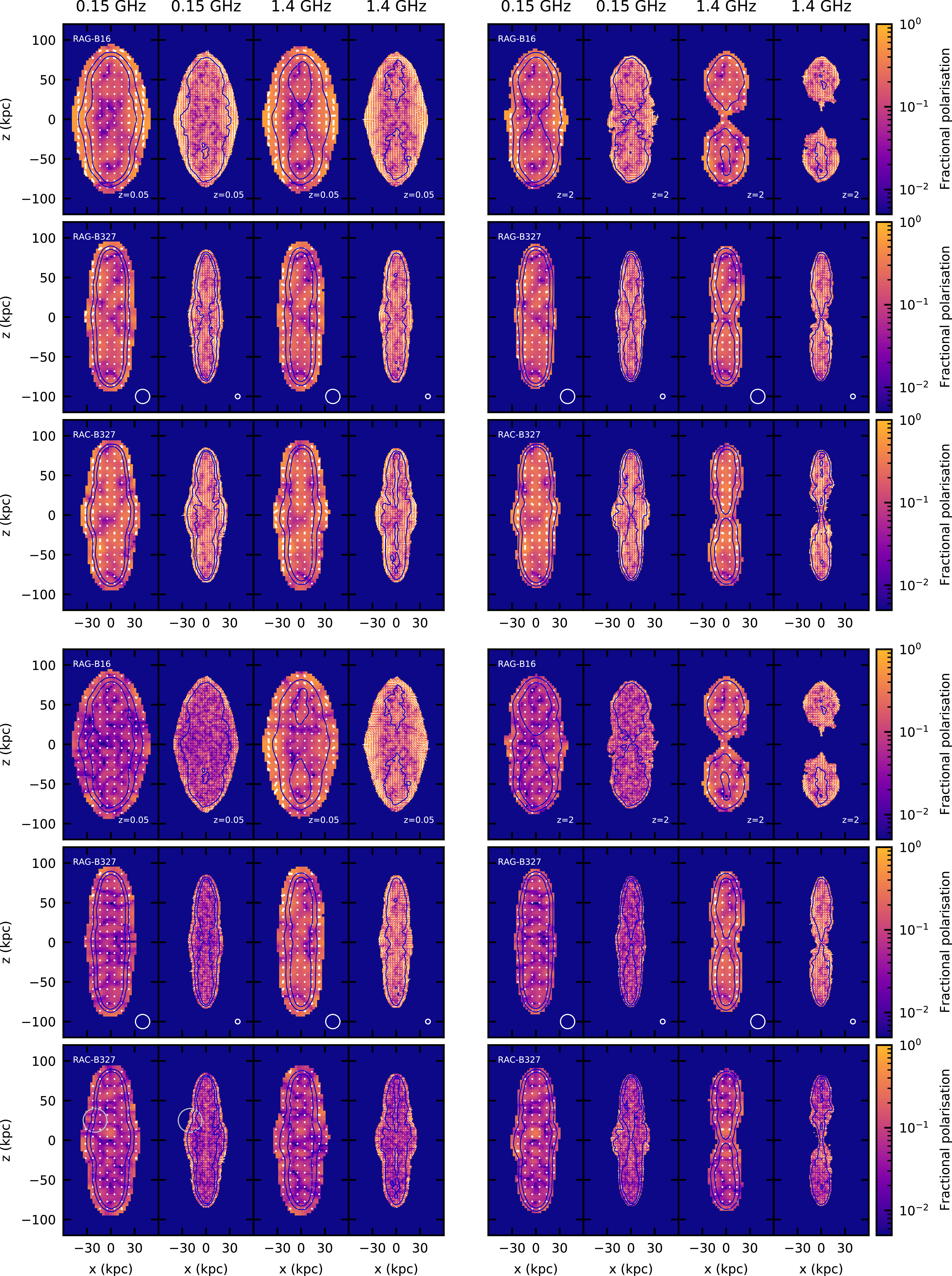
For each simulation, across all frequencies, redshifts, and resolutions, we find a patchy fractional polarisation structure. The fractional polarisation is higher towards the edges (on average roughly 50%), a feature that is consistent with observations of polarised radio lobes (Hogbom Reference Hogbom1979; Bridle et al. Reference Bridle, Hough, Lonsdale, Burns and Laing1994). This structure is smoothed out across the source in the lower resolution images, losing much of the detail given by the complex magnetic field present in the lobes. This also reduces the magnitude of the fractional polarisation through beam depolarisation.
The amount of beam depolarisation depends on the size of the patchy fractional polarisation structure and whether that is smaller than the beam size. In simulation RAG-B16, this depolarisation occurs primarily along the jet axis, where the patchy structure is clearly seen at high resolution. For simulation RAG-B327, this depolarisation effect is strongest near the origin, while another clear patch of beam depolarisation can be seen at about 40 kpc along the upper jet axis in Figure 11. The characteristics of the beam depolarisation are similar in simulation RAC-B327, but a clear example of this effect occurs at
 $x \simeq -10$
,
$x \simeq -10$
,
 $z \simeq 25$
, in a bright and highly polarised region (at high resolution) where the particles are being slowed down in the cocoon (as discussed in Section 3.3).
$z \simeq 25$
, in a bright and highly polarised region (at high resolution) where the particles are being slowed down in the cocoon (as discussed in Section 3.3).
In each simulation, we see that many of the vectors perpendicular to the polarisation angle (i.e. the ‘magnetic field direction’) are aligned primarily parallel to the jet axis, consistent with the structures seen in observations of radio lobes (Laing Reference Laing1980; Gilbert et al. Reference Gilbert2004). Simulations RAG-B327 and RAC-B327 do not show this feature as clearly due to the narrowness of their lobes as compared to the lobes in simulation RAG-B16. The magnetic field direction in simulation RAG-B16 is in general tangential to the lobe edge, a feature that has previously been found in simulations (Huarte-Espinosa et al. Reference Huarte-Espinosa, Krause and Alexander2011a). The narrow jets in simulations RAG-B327 and RAC-B327 do not show this feature at low resolution due to beam depolarisation.
At high resolution, we resolve more changes in the magnetic field direction on small scales. In each simulation, there is higher fractional polarisation at the edges of the lobes due to less smoothing of the patchy fractional polarisation structure by beam depolarisation. The magnetic field direction follows the jet flow in general, another feature commonly seen in radio lobe observations (e.g. Eilek & Owen Reference Eilek and Owen2002; Mullin, Hardcastle, & Riley Reference Mullin, Hardcastle and Riley2006; Sebokolodi et al. Reference Sebokolodi2020). The regions of high fractional polarisation, which are primarily at the lobe edges, do not correspond to the regions of bright Stokes I emission.
For simulation RAG-B16, we see that the fractional polarisation increases in the jet head region, as seen in observations of FR-II sources (Gilbert et al. Reference Gilbert2004; O’Sullivan et al. Reference O’Sullivan2018; Mahatma et al. Reference Mahatma2021). For simulation RAG-B327, we see an increase in fractional polarisation towards the northern jet head, however, as discussed in Section 3.3, the jet head region in this simulation is not clearly defined due to the destabilisation of the jet. We do not see an increase in fractional polarisation in the hotspot region for the southern jet in this simulation. Similarly, simulation RAC-B327 does not appear to show an increase in the fractional polarisation in the jet head region.
In the higher redshift images in the four columns on the right-hand side of Figure 11, we see less emission due to IC losses (as discussed in Section 3.3). In simulation RAG-B16 in particular, we see less emission from the high fractional polarisation lobe edges that were present at low redshift. The visible emission near the jet origin has a higher fractional polarisation than at low redshift for a low resolution, with a change in the magnetic field direction to be roughly
 $45^{\circ}$
from the jet axis, particularly in the northern jet. These changes with redshift are due to IC losses reducing the synchrotron emission in the equatorial region of the lobe and increasing the contribution from particles in the jet with high
$45^{\circ}$
from the jet axis, particularly in the northern jet. These changes with redshift are due to IC losses reducing the synchrotron emission in the equatorial region of the lobe and increasing the contribution from particles in the jet with high
 $u_B$
. This increases the overall fractional polarisation as the jet magnetic field is highly ordered compared to the lobe magnetic field.
$u_B$
. This increases the overall fractional polarisation as the jet magnetic field is highly ordered compared to the lobe magnetic field.
In the higher jet magnetic field simulations there are also higher fractional polarisation values near the origin at higher redshift, however, this difference in fractional polarisation is small compared to the difference seen for simulation RAG-B16. This is due to the strong synchrotron emission from the jet that is not as impacted by IC losses compared to the jet in simulation RAG-B16. The higher frequency of
 $1.4$
GHz shows greater losses for simulations RAG-B327 and RAC-B327, which again changes the magnetic field direction in the regions closest to the jet origin. For simulation RAC-B327, the magnetic field direction remains mostly unchanged, as seen in the region near
$1.4$
GHz shows greater losses for simulations RAG-B327 and RAC-B327, which again changes the magnetic field direction in the regions closest to the jet origin. For simulation RAC-B327, the magnetic field direction remains mostly unchanged, as seen in the region near
 $0 \lesssim x \lesssim 15, z \simeq -20$
kpc.
$0 \lesssim x \lesssim 15, z \simeq -20$
kpc.
In Figure 12, we plot the integrated fractional polarisation,
 $F_{\rm tot} = \sqrt{Q_{\rm tot}^2 + U_{\rm tot}^2}/I_{\rm tot}$
; i.e. the fractional polarisation that would be measured if the source was unresolved. We include three different viewing angles to the source:
$F_{\rm tot} = \sqrt{Q_{\rm tot}^2 + U_{\rm tot}^2}/I_{\rm tot}$
; i.e. the fractional polarisation that would be measured if the source was unresolved. We include three different viewing angles to the source:
 $0^{\circ}, 30^{\circ},$
and
$0^{\circ}, 30^{\circ},$
and
 $60^{\circ}$
to the plane of the sky. In this section, we do not consider the effects of Faraday rotation (these effects are discussed in Section 4.2).
$60^{\circ}$
to the plane of the sky. In this section, we do not consider the effects of Faraday rotation (these effects are discussed in Section 4.2).
Evolution of the integrated fractional polarisation over time for simulations RAG-B16 (top panel), RAG-B327 (middle panel), and RAC-B327 (bottom panel). Each simulation is plotted for three viewing angles (
 $0^{\circ}, 30^{\circ}, 60^{\circ}$
) and two redshifts (
$0^{\circ}, 30^{\circ}, 60^{\circ}$
) and two redshifts (
 $z = 0.05, 2$
). In the more saturated colours on the plot, we ignore the effects of Faraday rotation; Faraday rotation is applied for the desaturated colours.
$z = 0.05, 2$
). In the more saturated colours on the plot, we ignore the effects of Faraday rotation; Faraday rotation is applied for the desaturated colours.

 $F_{\rm tot}$
for our simulated sources are in general below 30% at all simulation times. For simulations in the group environment,
$F_{\rm tot}$
for our simulated sources are in general below 30% at all simulation times. For simulations in the group environment,
 $F_{\rm tot}$
initially decreases quickly (from up to 20% in simulation RAG-B327) for all viewing angles. This initial decline corresponds to the lobe formation phase, where the source is dominated by jet emission, which is highly polarised due to its coherent toroidal magnetic field and is less impacted by beam depolarisation. The redshift of the source does not significantly impact
$F_{\rm tot}$
initially decreases quickly (from up to 20% in simulation RAG-B327) for all viewing angles. This initial decline corresponds to the lobe formation phase, where the source is dominated by jet emission, which is highly polarised due to its coherent toroidal magnetic field and is less impacted by beam depolarisation. The redshift of the source does not significantly impact
 $F_{\rm tot}$
; for the higher jet magnetic field strength simulations, there appears to be a separation where the higher redshift sources have greater
$F_{\rm tot}$
; for the higher jet magnetic field strength simulations, there appears to be a separation where the higher redshift sources have greater
 $F_{\rm tot}$
, however, this difference is negligible.
$F_{\rm tot}$
, however, this difference is negligible.
The behaviour after this initial decrease is different between each of the simulations.
 $F_{\rm tot}$
in simulation RAG-B16 plateaus smoothly and remains around
$F_{\rm tot}$
in simulation RAG-B16 plateaus smoothly and remains around
 $9 \pm 1$
% after 5 Myr for all viewing angles and redshifts. Simulations RAG-B327 and RAC-B327 both have an increase between 2 and 5 Myr before plateauing, however, this increase is greater for the cluster simulation. After 5 Myr, at viewing angles of
$9 \pm 1$
% after 5 Myr for all viewing angles and redshifts. Simulations RAG-B327 and RAC-B327 both have an increase between 2 and 5 Myr before plateauing, however, this increase is greater for the cluster simulation. After 5 Myr, at viewing angles of
 $0^{\circ}$
and
$0^{\circ}$
and
 $30^{\circ}$
, simulation RAG-B327 has values of
$30^{\circ}$
, simulation RAG-B327 has values of
 $F_{\rm tot}$
around
$F_{\rm tot}$
around
 $11 \pm 2$
%, compared to
$11 \pm 2$
%, compared to
 $17 \pm 3$
% for simulation RAC-B327, indicating that the more confined jet in the cluster environment has a higher intrinsic polarisation once the large-scale radio lobe is fully formed. However, in observations, this will be offset by the greater depolarising effect of the cluster environment (as discussed in Section 4.2).
$17 \pm 3$
% for simulation RAC-B327, indicating that the more confined jet in the cluster environment has a higher intrinsic polarisation once the large-scale radio lobe is fully formed. However, in observations, this will be offset by the greater depolarising effect of the cluster environment (as discussed in Section 4.2).
For the higher jet magnetic field strength simulations, the behaviour at an oblique viewing angle of
 $60^{\circ}$
is similar to each other, in that
$60^{\circ}$
is similar to each other, in that
 $F_{\rm tot}$
is trending downwards with great scatter (with values ranging between
$F_{\rm tot}$
is trending downwards with great scatter (with values ranging between
 $5 \pm 4$
% for simulation RAG-B327 and
$5 \pm 4$
% for simulation RAG-B327 and
 $11 \pm 4$
% for simulation RAC-B327). These sources appear quite compact at this oblique viewing angle due to the narrowness of the jet cocoon, which increases the visible amount of the lobe edge (which has high fractional polarisation; Laing Reference Laing1980) in comparison to the total source size. This high fractional polarisation gets averaged out in the integration across I, Q, and U when calculating
$11 \pm 4$
% for simulation RAC-B327). These sources appear quite compact at this oblique viewing angle due to the narrowness of the jet cocoon, which increases the visible amount of the lobe edge (which has high fractional polarisation; Laing Reference Laing1980) in comparison to the total source size. This high fractional polarisation gets averaged out in the integration across I, Q, and U when calculating
 $F_{\rm tot}$
.
$F_{\rm tot}$
.
Despite each simulation showing a clear initial decrease in
 $F_{\rm tot}$
, the initial value is generally lower than for past polarisation estimates from simulations (Hardcastle & Krause Reference Hardcastle and Krause2014; English et al. Reference English, Hardcastle and Krause2016). We also find much smaller changes in the integrated fractional polarisation over time; both Hardcastle & Krause (Reference Hardcastle and Krause2014) and English et al. (Reference English, Hardcastle and Krause2016) find a decrease from the initial maximum fractional polarisation of approximately 70% to 0% for lobes that evolve to 300 kpc scales. The higher
$F_{\rm tot}$
, the initial value is generally lower than for past polarisation estimates from simulations (Hardcastle & Krause Reference Hardcastle and Krause2014; English et al. Reference English, Hardcastle and Krause2016). We also find much smaller changes in the integrated fractional polarisation over time; both Hardcastle & Krause (Reference Hardcastle and Krause2014) and English et al. (Reference English, Hardcastle and Krause2016) find a decrease from the initial maximum fractional polarisation of approximately 70% to 0% for lobes that evolve to 300 kpc scales. The higher
 $F_{\rm tot}$
in simulation RAC-B327 indicates that a denser environment can lead to higher intrinsic polarisation of the source; the simulations discussed in Hardcastle & Krause (Reference Hardcastle and Krause2014) and English et al. (Reference English, Hardcastle and Krause2016) have a greater central density of
$F_{\rm tot}$
in simulation RAC-B327 indicates that a denser environment can lead to higher intrinsic polarisation of the source; the simulations discussed in Hardcastle & Krause (Reference Hardcastle and Krause2014) and English et al. (Reference English, Hardcastle and Krause2016) have a greater central density of
 $3 \times 10^{-26}$
g/cm
$3 \times 10^{-26}$
g/cm
 $^3$
compared to
$^3$
compared to
 $1.5 \times 10^{-26}$
g/cm
$1.5 \times 10^{-26}$
g/cm
 $^3$
and
$^3$
and
 $4.2 \times 10^{-27}$
g/cm
$4.2 \times 10^{-27}$
g/cm
 $^3$
in our cluster and group environments, respectively. This difference in environment is likely the main cause of the difference in the integrated fractional polarisation over time, however, the difference in how the polarised emission is calculated will also contribute (see Section 4.3).
$^3$
in our cluster and group environments, respectively. This difference in environment is likely the main cause of the difference in the integrated fractional polarisation over time, however, the difference in how the polarised emission is calculated will also contribute (see Section 4.3).
In contrast, we find in Figure 13 that the mean fractional polarisation, i.e. the mean value of
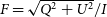 $F = \sqrt{Q^2 + U^2}/I$
(as plotted in Figure 11), shows less evolution over time. We find that redshift and viewing angle impact the mean fractional polarisation for all our simulations. Like for the integrated fractional polarisation plot, we leave the discussion of the effects of Faraday rotation for Section 4.2. For simulation RAG-B16, we see that the mean fractional polarisation is higher at lower redshifts for all viewing angles. When viewed at an angle of
$F = \sqrt{Q^2 + U^2}/I$
(as plotted in Figure 11), shows less evolution over time. We find that redshift and viewing angle impact the mean fractional polarisation for all our simulations. Like for the integrated fractional polarisation plot, we leave the discussion of the effects of Faraday rotation for Section 4.2. For simulation RAG-B16, we see that the mean fractional polarisation is higher at lower redshifts for all viewing angles. When viewed at an angle of
 $60^{\circ}$
, the mean fractional polarisation is generally lower than when the source is viewed at a less oblique angle.
$60^{\circ}$
, the mean fractional polarisation is generally lower than when the source is viewed at a less oblique angle.
Evolution of the mean fractional polarisation over time for simulations RAG-B16 (top panel), RAG-B327 (middle panel), and RAC-B327 (bottom panel). Each simulation is plotted for three viewing angles (
 $0^{\circ}, 30^{\circ}, 60^{\circ}$
) and two redshifts (
$0^{\circ}, 30^{\circ}, 60^{\circ}$
) and two redshifts (
 $z = 0.05, 2$
). In the more saturated colours on the plot, we ignore the effects of Faraday rotation; Faraday rotation is applied for the desaturated colours.
$z = 0.05, 2$
). In the more saturated colours on the plot, we ignore the effects of Faraday rotation; Faraday rotation is applied for the desaturated colours.
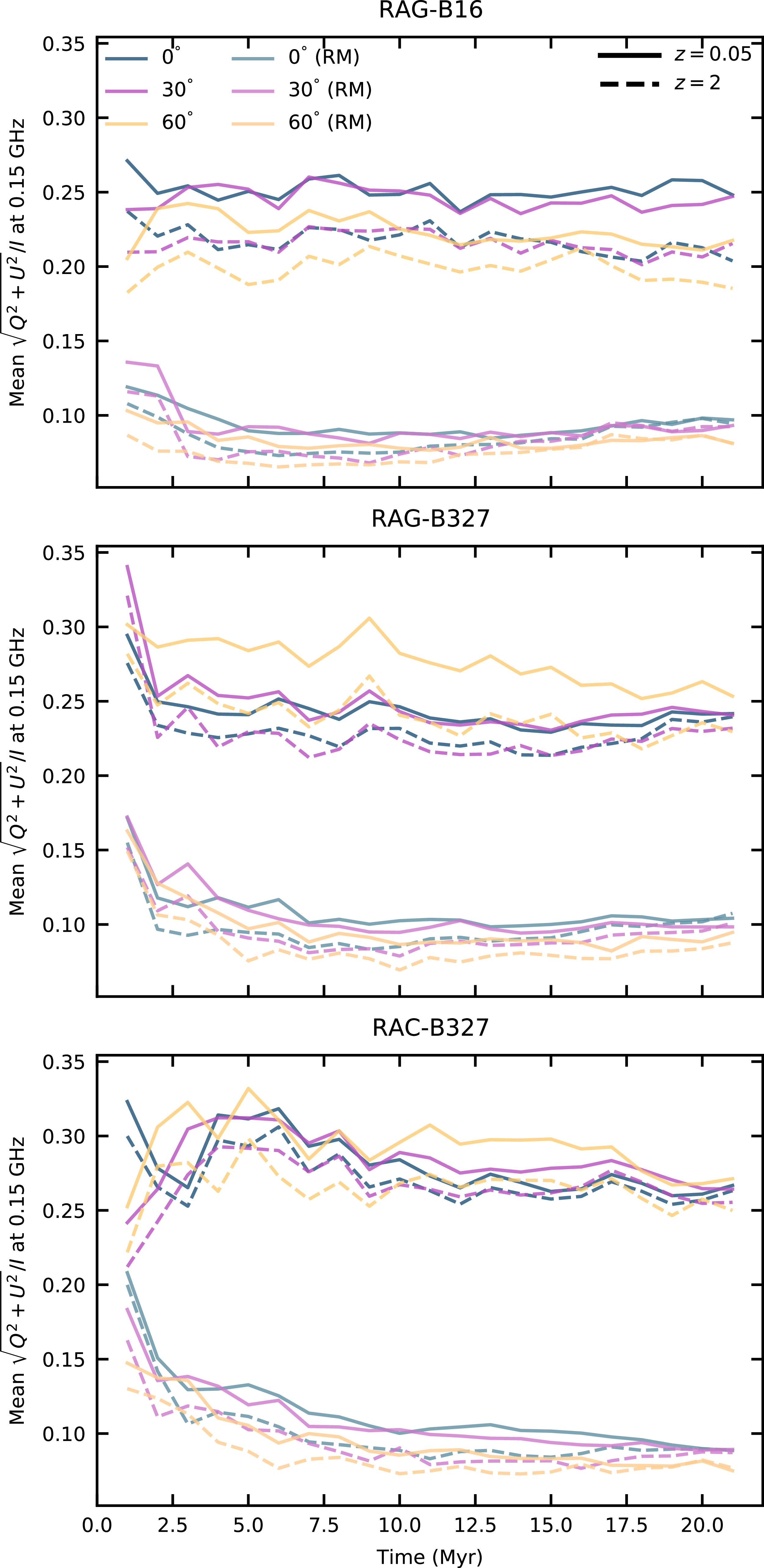
In simulations RAG-B327 and RAC-B327, we have an initial decrease of the mean fractional polarisation in the first 2 Myr, followed by a plateau; this corresponds to the lobe formation phase. In contrast to simulation RAG-B16, we find that for the
 $60^{\circ}$
viewing angle the mean fractional polarisation is in general the same or higher, e.g. the low-redshift case in simulation RAG-B327. This increase with viewing angle compared to simulation RAG-B16 is due to the morphology of the highly magnetised sources; due to their narrowness, when they are viewed at an oblique angle, the edges of the lobe (which in general have the highest fractional polarisation) contribute more to increasing the mean fractional polarisation. For simulation RAG-B327 we also see the clear difference in redshift seen for simulation RAG-B16 at a viewing angle of
$60^{\circ}$
viewing angle the mean fractional polarisation is in general the same or higher, e.g. the low-redshift case in simulation RAG-B327. This increase with viewing angle compared to simulation RAG-B16 is due to the morphology of the highly magnetised sources; due to their narrowness, when they are viewed at an oblique angle, the edges of the lobe (which in general have the highest fractional polarisation) contribute more to increasing the mean fractional polarisation. For simulation RAG-B327 we also see the clear difference in redshift seen for simulation RAG-B16 at a viewing angle of
 $60^{\circ}$
, however, it is not present for less oblique viewing angles or in simulation RAC-B327.
$60^{\circ}$
, however, it is not present for less oblique viewing angles or in simulation RAC-B327.
Hardcastle & Krause (Reference Hardcastle and Krause2014) and English et al. (Reference English, Hardcastle and Krause2016) also find that the mean fractional polarisation evolves more slowly over time compared to
 $F_{\rm tot}$
; however, these authors find much greater decreases over time. We also note that the mean fractional polarisations found by these authors do not drop below 30% at any point, indicating that the BRAiSE method in general produces sources with lower fractional polarisation compared to these previous estimates. As discussed earlier, this is likely due to a combination of differences in the environment and the polarisation calculation for these simulated sources. In contrast, the mean fractional polarisation evolution found by Meenakshi et al. (Reference Meenakshi, Mukherjee, Bodo and Rossi2023) decreases from approximately 68% to 36% after
$F_{\rm tot}$
; however, these authors find much greater decreases over time. We also note that the mean fractional polarisations found by these authors do not drop below 30% at any point, indicating that the BRAiSE method in general produces sources with lower fractional polarisation compared to these previous estimates. As discussed earlier, this is likely due to a combination of differences in the environment and the polarisation calculation for these simulated sources. In contrast, the mean fractional polarisation evolution found by Meenakshi et al. (Reference Meenakshi, Mukherjee, Bodo and Rossi2023) decreases from approximately 68% to 36% after
 $0.6$
Myr, which is consistent with the initial sharp decrease we find in simulation RAG-B327. Since the simulations performed by Meenakshi et al. (Reference Meenakshi, Mukherjee, Bodo and Rossi2023) are only run on short timescales in comparison to this work, and follow much smaller lobe sizes, we would expect that their mean fractional polarisation would continue to decrease as we have shown for simulations RAG-B327 and RAC-B327.
$0.6$
Myr, which is consistent with the initial sharp decrease we find in simulation RAG-B327. Since the simulations performed by Meenakshi et al. (Reference Meenakshi, Mukherjee, Bodo and Rossi2023) are only run on short timescales in comparison to this work, and follow much smaller lobe sizes, we would expect that their mean fractional polarisation would continue to decrease as we have shown for simulations RAG-B327 and RAC-B327.
4.2 Depolarisation due to Faraday rotation
The polarised emission from AGN jet sources is depolarised by Faraday rotation, which depends on the environment the source resides in (e.g. Jerrim et al. Reference Jerrim2024). We calculate the Faraday RM by integrating Equation (2) along a rotated grid for each Lagrangian tracer particle on the simulation grid, using the grid fluid variables, following the method outlined in Jerrim et al. (Reference Jerrim2024). We assign the final RM value to each particle, which is then used to rotate the polarisation angle using Equation (1), where the initial polarisation angle is found following Equation (13). This method accounts for both external and internal Faraday rotation, which will result in Faraday depolarisation.
The Faraday rotation measures for each particle are shown in Figure 14. Simulation RAC-B327 has much greater RM values than the group simulations due to the higher density and magnetic field strength in the cluster environment. Particles towards the edges of the lobes generally have higher RM values; this is due to the alignment of the magnetic field that is pushed out by the jet cocoon with the line of sight (Huarte-Espinosa et al. Reference Huarte-Espinosa, Krause and Alexander2011b). Otherwise, since the magnetic field structure in the ambient environment is the same, there are no major differences in the spatial structures shown in these RM maps. We note that as the viewing angle to the source is increased, the difference in RM magnitude between the upper (closer) jet and lower (further away) jet changes significantly.
Particle RM maps for the RMHD simulations. Each simulation is plotted with three viewing angles (
 $0^{\circ}, 30^{\circ}, 60^{\circ}$
). Top row: simulation RAG-B16. Middle row: simulation RAG-B327. Bottom row: simulation RAC-B327.
$0^{\circ}, 30^{\circ}, 60^{\circ}$
). Top row: simulation RAG-B16. Middle row: simulation RAG-B327. Bottom row: simulation RAC-B327.

We plot the fractional polarisation with Faraday rotation applied in the lower half of Figure 11. There is a clear reduction in the fractional polarisation across each map for each simulation due to Faraday depolarisation at
 $0.15$
GHz. The patchy structures have smaller scales, which is particularly noticeable for the higher image resolution. In simulations RAG-B16 and RAC-B327 at high redshift, we still see the region of increased fractional polarisation near the origin. The vectors perpendicular to the polarisation angle (i.e. what the inferred ‘magnetic field direction’ is for no Faraday rotation in the high-frequency limit) are no longer tangential to the lobe edges in each simulation; in general, there is no consistency with the magnetic field directions seen in the upper half of Figure 11. The polarised emission in the group simulations (RAG-B16 and RAG-B327) is not as strongly depolarised as in the cluster simulation (RAC-B327).
$0.15$
GHz. The patchy structures have smaller scales, which is particularly noticeable for the higher image resolution. In simulations RAG-B16 and RAC-B327 at high redshift, we still see the region of increased fractional polarisation near the origin. The vectors perpendicular to the polarisation angle (i.e. what the inferred ‘magnetic field direction’ is for no Faraday rotation in the high-frequency limit) are no longer tangential to the lobe edges in each simulation; in general, there is no consistency with the magnetic field directions seen in the upper half of Figure 11. The polarised emission in the group simulations (RAG-B16 and RAG-B327) is not as strongly depolarised as in the cluster simulation (RAC-B327).
At
 $1.4$
GHz the fractional polarisation is slightly reduced for the group simulations (as compared to Figure 11), but this effect is more subtle than for the lower frequency. Simulation RAC-B327 shows significant depolarisation at
$1.4$
GHz the fractional polarisation is slightly reduced for the group simulations (as compared to Figure 11), but this effect is more subtle than for the lower frequency. Simulation RAC-B327 shows significant depolarisation at
 $1.4$
GHz. Since this simulation has a cluster environment with both a higher density and a higher average cluster magnetic field strength, the RMs have a wider range of values and hence the depolarisation effect is stronger at higher frequencies, as predicted in Jerrim et al. (Reference Jerrim2024). Simulation RAC-B327 has higher fractional polarisation areas at the edges of the lobe close to where the lobe is mixing with the shocked ambient medium (e.g. at
$1.4$
GHz. Since this simulation has a cluster environment with both a higher density and a higher average cluster magnetic field strength, the RMs have a wider range of values and hence the depolarisation effect is stronger at higher frequencies, as predicted in Jerrim et al. (Reference Jerrim2024). Simulation RAC-B327 has higher fractional polarisation areas at the edges of the lobe close to where the lobe is mixing with the shocked ambient medium (e.g. at
 $x \simeq -20$
,
$x \simeq -20$
,
 $z \simeq 25$
), since the magnetic field at the edge of the lobe will be preferentially aligned with the line of sight due to the geometry of the jet cocoon, which is amplified more for wider cocoons (Huarte-Espinosa et al. Reference Huarte-Espinosa, Krause and Alexander2011b). This effect is lessened in simulation RAG-B327 due to its narrow cocoon.
$z \simeq 25$
), since the magnetic field at the edge of the lobe will be preferentially aligned with the line of sight due to the geometry of the jet cocoon, which is amplified more for wider cocoons (Huarte-Espinosa et al. Reference Huarte-Espinosa, Krause and Alexander2011b). This effect is lessened in simulation RAG-B327 due to its narrow cocoon.
Both the integrated and the mean fractional polarisation over time is reduced when the RM is applied (see the desaturated lines in Figures 12, 13). The integrated fractional polarisation in simulation RAG-B16 falls below 5% within the first few Myr, indicating that this source is almost entirely unpolarised at
 $0.15$
GHz. In simulations RAG-B327 and RAC-B327 for a viewing angle of
$0.15$
GHz. In simulations RAG-B327 and RAC-B327 for a viewing angle of
 $60^{\circ}$
, the integrated fractional polarisation over time is higher than that for smaller viewing angles. This behaviour is the opposite to that seen without Faraday depolarisation. At viewing angles of
$60^{\circ}$
, the integrated fractional polarisation over time is higher than that for smaller viewing angles. This behaviour is the opposite to that seen without Faraday depolarisation. At viewing angles of
 $0^{\circ}$
and
$0^{\circ}$
and
 $30^{\circ}$
, the source is mostly unpolarised. This dramatic change in the polarisation is because the northern jet in both simulations is not strongly depolarised by Faraday rotation due to its comparatively lower RMs than the southern jet (see Figure 14), meaning the overall fractional polarisation is higher. In simulation RAC-B327, the greater RMs result in greater depolarisation of the jet emission than in simulation RAG-B327, however, the lobe edges in the cluster simulation have greater fractional polarisation values due to the alignment of the magnetic field with the cocoon.
$30^{\circ}$
, the source is mostly unpolarised. This dramatic change in the polarisation is because the northern jet in both simulations is not strongly depolarised by Faraday rotation due to its comparatively lower RMs than the southern jet (see Figure 14), meaning the overall fractional polarisation is higher. In simulation RAC-B327, the greater RMs result in greater depolarisation of the jet emission than in simulation RAG-B327, however, the lobe edges in the cluster simulation have greater fractional polarisation values due to the alignment of the magnetic field with the cocoon.
The mean fractional polarisation in all our simulations remains consistent after the initial decrease. After the lobe formation phase is complete (
 $\gt 5$
Myr), the mean fractional polarisation over all viewing angles and redshifts in simulations RAG-B16, RAG-B327, and RAC-B327 drops from
$\gt 5$
Myr), the mean fractional polarisation over all viewing angles and redshifts in simulations RAG-B16, RAG-B327, and RAC-B327 drops from
 $22 \pm 2$
%,
$22 \pm 2$
%,
 $24 \pm 2$
% and
$24 \pm 2$
% and
 $27 \pm 2$
% without Faraday depolarisation to
$27 \pm 2$
% without Faraday depolarisation to
 $8.3 \pm 0.8$
%,
$8.3 \pm 0.8$
%,
 $9.2 \pm 0.9$
% and
$9.2 \pm 0.9$
% and
 $9 \pm 1$
% when Faraday depolarisation is applied. The decrease in mean fractional polarisation is greatest for simulation RAC-B327 due to its higher density cluster environment and therefore higher RM values (e.g. Jerrim et al. Reference Jerrim2024).
$9 \pm 1$
% when Faraday depolarisation is applied. The decrease in mean fractional polarisation is greatest for simulation RAC-B327 due to its higher density cluster environment and therefore higher RM values (e.g. Jerrim et al. Reference Jerrim2024).
Hardcastle & Krause (Reference Hardcastle and Krause2014) study the Laing-Garrington effect in their simulations using a depolarisation ratio (DPR), measured as a ratio of the depolarisation of the jet and counterjet. This depolarisation for each jet is the ratio of polarised flux density (with Faraday rotation applied) for a low and high frequency, respectively; Hardcastle & Krause (Reference Hardcastle and Krause2014) choose frequencies of
 $1.4$
and
$1.4$
and
 $5.0$
GHz. The DPR should be greater than 1 if the jet (pointed towards the observer) is less depolarised than its counterjet (pointed away from the observer), as expected from the Laing-Garrington effect (Laing Reference Laing1988; Garrington et al. Reference Garrington, Leahy, Conway and Laing1988). This is due to the fact that the jet that is pointed towards the observer will have lower Faraday rotation measure values as there will be a shorter path length through the shocked shell of ambient medium that surrounds the jet cocoon (e.g. Jerrim et al. Reference Jerrim2024).
$5.0$
GHz. The DPR should be greater than 1 if the jet (pointed towards the observer) is less depolarised than its counterjet (pointed away from the observer), as expected from the Laing-Garrington effect (Laing Reference Laing1988; Garrington et al. Reference Garrington, Leahy, Conway and Laing1988). This is due to the fact that the jet that is pointed towards the observer will have lower Faraday rotation measure values as there will be a shorter path length through the shocked shell of ambient medium that surrounds the jet cocoon (e.g. Jerrim et al. Reference Jerrim2024).
We plot the DPR for
 $1.4$
and
$1.4$
and
 $5.5$
GHz in Figure 15. For viewing angles
$5.5$
GHz in Figure 15. For viewing angles
 $\gt 0 ^{\circ}$
in our group simulations, the DPR is in general
$\gt 0 ^{\circ}$
in our group simulations, the DPR is in general
 $\gt 1$
, consistent with our expectations from the differences in RM magnitudes (Figure 14) and the Laing-Garrington effect. However, the DPR is not always
$\gt 1$
, consistent with our expectations from the differences in RM magnitudes (Figure 14) and the Laing-Garrington effect. However, the DPR is not always
 $\gt 1$
due to the differences in the turbulent magnetic field structure along the line of sight, which change with viewing angle. DPR values
$\gt 1$
due to the differences in the turbulent magnetic field structure along the line of sight, which change with viewing angle. DPR values
 $\lt 1$
are more common for a viewing angle of
$\lt 1$
are more common for a viewing angle of
 $0 ^{\circ}$
, as there is no significant difference in the RM magnitude between the jets. The scatter in DPR values is much greater over time (up to a factor of 10 times greater values) than those seen by Hardcastle & Krause (Reference Hardcastle and Krause2014); we compare multiple viewing angles to the radio lobes, whereas they consider their lobes at a viewing angle of
$0 ^{\circ}$
, as there is no significant difference in the RM magnitude between the jets. The scatter in DPR values is much greater over time (up to a factor of 10 times greater values) than those seen by Hardcastle & Krause (Reference Hardcastle and Krause2014); we compare multiple viewing angles to the radio lobes, whereas they consider their lobes at a viewing angle of
 $45^{\circ}$
only. Our cluster simulation shows much greater scatter for all viewing angles since it is partially depolarised at
$45^{\circ}$
only. Our cluster simulation shows much greater scatter for all viewing angles since it is partially depolarised at
 $5.5$
GHz, in comparison to the group simulations which are not depolarised at that frequency.
$5.5$
GHz, in comparison to the group simulations which are not depolarised at that frequency.
Evolution of the depolarisation ratio over time for simulations RAG-B16 (top panel), RAG-B327 (middle panel), and RAC-B327 (bottom panel). Each simulation is plotted for three viewing angles (
 $0^{\circ}, 30^{\circ}, 60^{\circ}$
) and two redshifts (
$0^{\circ}, 30^{\circ}, 60^{\circ}$
) and two redshifts (
 $z = 0.05, 2$
). The horizontal grey line indicates a DPR of 1.
$z = 0.05, 2$
). The horizontal grey line indicates a DPR of 1.
4.3 Comparison of Stokes parameters to previous work
Our fractional polarisation maps are calculated from the Stokes parameters following Equation (14). We compare our Stokes Q and U parameters qualitatively with previous images rendered by Hardcastle & Krause (Reference Hardcastle and Krause2014) and English et al. (Reference English, Hardcastle and Krause2016) to understand the differences between this previous method for calculating the Stokes parameters and our new method which uses an evolving electron energy distribution. English et al. (Reference English, Hardcastle and Krause2016) use modified Stokes parameters that take into account aberration effects in relativistic fluids. Here, we follow English et al. (Reference English, Hardcastle and Krause2016) to calculate the Stokes parameters for our Lagrangian particles:
 \begin{align}\begin{split} j_I &= p(B_x^2 + B_z^2)^{(\alpha - 1)/2} (B_x^2 + B_z^2) D^{3 + \alpha}, \\ j_Q &= \mu_P p(B_x^2 + B_z^2)^{(\alpha - 1)/2} (B_x^2 - B_z^2) D^{3 + \alpha}, \\ j_U &= \mu_P p(B_x^2 + B_z^2)^{(\alpha - 1)/2} (2B_xB_z) D^{3 + \alpha}. \end{split}\end{align}
Here, the maximum fractional polarisation
 $\mu_P = (\alpha + 1)/(\alpha + 5/3)$
, and the Doppler factor
$\mu_P = (\alpha + 1)/(\alpha + 5/3)$
, and the Doppler factor
 $D = 1/(\gamma (1 - \beta \cos\theta))$
, where
$D = 1/(\gamma (1 - \beta \cos\theta))$
, where
 $\beta = v/c$
and
$\beta = v/c$
and
 $\theta$
is the angle between the line of sight and the velocity vector of the cell. We integrate the emissivities
$\theta$
is the angle between the line of sight and the velocity vector of the cell. We integrate the emissivities
 $j_I, j_Q,$
and
$j_I, j_Q,$
and
 $j_U$
for the particles along the line of sight on the grid, in the same manner as outlined in Yates-Jones et al. (Reference Yates-Jones, Turner, Shabala and Krause2022) and plot Stokes Q, U, and
$j_U$
for the particles along the line of sight on the grid, in the same manner as outlined in Yates-Jones et al. (Reference Yates-Jones, Turner, Shabala and Krause2022) and plot Stokes Q, U, and
 $\sqrt{Q^2 +U^2}$
for each of our RMHD simulations in the left panel of Figure 16. For consistency with our Stokes parameters, we scale the magnetic field by the volume filling factor as
$\sqrt{Q^2 +U^2}$
for each of our RMHD simulations in the left panel of Figure 16. For consistency with our Stokes parameters, we scale the magnetic field by the volume filling factor as
 $B' = B / \sqrt{\rm trc}$
and multiply the Stokes emissivities by the volume filling factor from Equation (8) for this calculation. We plot our Stokes Q and U parameters in the right panel of Figure 16, where the parameters are calculated as detailed in Equation (12). For each of the calculation methods, we see the typical patchy effect from the complex magnetic field seen in Figure 11.
$B' = B / \sqrt{\rm trc}$
and multiply the Stokes emissivities by the volume filling factor from Equation (8) for this calculation. We plot our Stokes Q and U parameters in the right panel of Figure 16, where the parameters are calculated as detailed in Equation (12). For each of the calculation methods, we see the typical patchy effect from the complex magnetic field seen in Figure 11.
Stokes’ parameters (Q, U,
 $\sqrt{Q^2+U^2}$
) for simulations RAG-B16 (top row), RAG-B327 (middle row), and RAC-B327 (bottom row). Left: Stokes’ parameters calculated using the method outlined in English et al. (Reference English, Hardcastle and Krause2016). Right: Stokes’ parameters calculated using the method described in this paper.
$\sqrt{Q^2+U^2}$
) for simulations RAG-B16 (top row), RAG-B327 (middle row), and RAC-B327 (bottom row). Left: Stokes’ parameters calculated using the method outlined in English et al. (Reference English, Hardcastle and Krause2016). Right: Stokes’ parameters calculated using the method described in this paper.

Using the method described in this paper, we find that for simulation RAG-B16, there are minimal differences between the Stokes Q and U parameters between the two different calculation methods. However, for the higher jet magnetic field simulations, there are minor differences in both Stokes Q and U; in general, the images are broadly consistent with one another. For the English et al. (Reference English, Hardcastle and Krause2016) method, Stokes Q is in general more positive across the lobe, and the negative jet emission does not dominate as strongly as compared to our method. The Stokes U maps for the two methods have a similar distribution of positive and negative emission in the opposite sense to each other, due to a difference in sign between Equations (13) and (16); this sign difference does not affect the morphology of the structures.
The differences seen for our higher jet magnetic field simulations are due to the different dynamics between these simulations and simulation RAG-B16; the jets with a higher magnetic field strength are more stable to deceleration. Simulations RAG-B327 and RAC-B327 both have disrupted but not fully decelerated jets and therefore relativistic effects will be important for the synthetic polarisation calculation. We conclude that the stability of the jet impacts calculation of the Stokes parameters using the English et al. (Reference English, Hardcastle and Krause2016) method due to the relativistic effects on the polarisation position angle.
5. Conclusions
Using three-dimensional RMHD simulations of AGN jets and an extension for the synchrotron emission code PRAiSE (Yates-Jones et al. Reference Yates-Jones, Turner, Shabala and Krause2022), known as BRAiSE, we have demonstrated that the details of simulated radio synchrotron emission from AGN jets depends on whether the magnetic field or pressure is used to calculate it. This is due to the different distribution of magnetic energy density and pressure values throughout the lobe. This impacts both the spatial distribution of emission and the overall luminosity, thereby affecting the morphology and FR classification of the radio source. We also use the new BRAiSE method to study the polarisation properties of our simulated sources and the depolarising effect of Faraday rotation in both group and cluster environments.
High resolution surface brightness images produced using BRAiSE show clumps due to the complex magnetic field structure in the lobe. In general, BRAiSE produces sources with greater total luminosity due to the variation of magnetic field strength across the lobes. We simulate three sources; one that resembles a lobed FR-I source, and two that resemble FR-II sources. BRAiSE produces a diffuse hotspot region in our FR-II-like sources, since the magnetic energy at the jet head is spread out due to kink instabilities in the jet. BRAiSE also produces strong emission in a flaring point for these sources, which affects their classification using the FR index. We find that for PRAiSE, the FR index classifies each of our sources as an FR-II. However, for BRAiSE, these sources are more borderline. For our highly magnetised jets, BRAiSE predicts significantly lower FR indices than PRAiSE. We conclude that magnetic field information is required to interpret the FR morphology, and that our simulations show unique shock structures with the presence of both a flaring point and a hotspot that result in a bimodal surface brightness distribution. This unique shock structure indicates that we have not simulated true FR-II sources, and that our jet setup is missing the full set of physics required to stabilise the jet on large scales (e.g. jet rotation; Bodo et al. Reference Bodo, Mamatsashvili, Rossi and Mignone2016; Bodo et al. Reference Bodo, Mamatsashvili, Rossi and Mignone2019).
Using BRAiSE, we have calculated Stokes I, Q, and U images for each of our RMHD simulations. For low and high resolutions and redshifts, we find patchy regions of high fractional polarisation. Over time, for each simulation, we find that the integrated fractional polarisation is lowest for sources viewed at an oblique angle. For our simulation with a lower jet magnetic field, this trend holds for the mean fractional polarisation. However, for our simulations with a higher jet magnetic field, the mean fractional polarisation is highest for this oblique viewing angle. This is due to the narrow morphology of these strongly magnetised sources.
Using Faraday rotation measures, we study the effect of depolarisation for our polarised sources: depolarisation is strongest at low frequencies, as expected. We confirm the Laing-Garrington effect for our group simulations, in that the upper radio lobes are in general less depolarised than the receding radio lobes. For our cluster simulation, we find that the RM values are higher and thus the Faraday depolarisation is a stronger effect than in the group environment for frequencies ranging between
 $0.15$
–
$0.15$
–
 $5.5$
GHz, confirming the result from Jerrim et al. (Reference Jerrim2024).
$5.5$
GHz, confirming the result from Jerrim et al. (Reference Jerrim2024).
The method we use to calculate the Stokes Q and U is different to a previous method used by Huarte-Espinosa et al. (Reference Huarte-Espinosa, Krause and Alexander2011a), Hardcastle & Krause (Reference Hardcastle and Krause2014), and English et al. (Reference English, Hardcastle and Krause2016). We qualitatively compare the differences between the two methods for our simulations, finding that our simulations with a higher jet magnetic field strength display minor differences in their Stokes Q and U maps, however, the simulation with a low magnetic field strength is almost identical. This demonstrates that the relativistic aberration effects should be accounted for in simulations of relativistic radio lobes.
Characterisation of magnetic field structure and synchrotron emissivity enabled by our RMHD simulations and analysis permits investigations of several other aspects of radio galaxy physics. We will compare and contrast more of the Stokes I spectral properties in our next paper. This and future work will be used in the CosmoDRAGoN project (Yates-Jones et al. Reference Yates-Jones2023) to study the synthetic emission of RMHD jets in realistic, magnetised, cluster environments. This project will provide insights on the link between observed radio AGN sources and the underlying physical mechanisms of AGN jet feedback in galaxy clusters.
Acknowledgements
LJ thanks the University of Tasmania for an Australian Government Research Training Program (RTP) Scholarship. SS, CP, and PYJ acknowledge funding by the Australian Research Council via grant DP240102970. This research was carried out using the high-performance computing clusters provided by Digital Research Services, IT Services at the University of Tasmania. This work has made use of data from The Three Hundred collaboration (https://www.the300-project.org) which benefits from financial support of the European Union’s Horizon 2020 Research and Innovation programme under the Marie Skłodowskaw-Curie grant agreement number 734374, that is the LACEGAL project. The Three Hundred simulations used in this paper have been performed in the MareNostrum Supercomputer at the Barcelona Supercomputing Center, thanks to CPU time granted by the Red Española de Supercomputación. We thank Knapen et al. (Reference Knapen, Chamba and Black2022) for their guide to writing astronomy papers. We acknowledge the support of the developers providing the Python packages used in this paper: Astropy (Astropy Collaboration et al. Reference Collaboration2022), JupyterLab (Kluyver et al. Reference Kluyver2016), Matplotlib (Hunter Reference Hunter2007), NumPy (Harris et al. Reference Harris2020), and SciPy (Virtanen et al. Reference Virtanen2020).
Data availability statement
The data underlying this article will be shared on reasonable request to the corresponding author.
Appendix A. Plasma composition
The fluid tracer in PLUTO describes the fraction (by mass) of radiating fluid within a grid cell in the simulation compared to the non-radiating (thermal) fluid. The passive Lagrangian particles record the history of the fluid values (including the tracer value and vector magnetic field) as they are advected with the fluid on the simulation grid. To calculate the synchrotron emission from these particles, we are interested in the fraction of this particle that is radiating.
PRAiSE (left two panels) and BRAiSE (right two panels) surface brightnesses (Stokes’ I) for the RAG-B327 simulation at 8 Myr,
 $z = 0.05$
, and
$z = 0.05$
, and
 $0.15$
GHz. Contours are at
$0.15$
GHz. Contours are at
 $1, 3.72, 13.9, 51.8, 193, 720, 2\,683,$
and
$1, 3.72, 13.9, 51.8, 193, 720, 2\,683,$
and
 $10\,000$
mJy/beam. Two plasma compositions are considered: ‘normal’ (mass ratio
$10\,000$
mJy/beam. Two plasma compositions are considered: ‘normal’ (mass ratio
 $ = 1$
) and ‘pair’ (mass ratio
$ = 1$
) and ‘pair’ (mass ratio
 $= 9 \times 10^{-4}$
).
$= 9 \times 10^{-4}$
).

Therefore, the synchrotron emissivity weighting depends on the assumed mass ratio between the radiating and thermal plasmas. For an electron-proton (‘normal’) plasma, this ratio is unity (as
 $m_r = m_{th} = \mu m_p$
), the volume filling factor simplifies to
$m_r = m_{th} = \mu m_p$
), the volume filling factor simplifies to
 $f = {\rm trc}$
, and the emissivity of each particle is simply weighted by its tracer value. This is the approach implemented in Yates-Jones et al. (Reference Yates-Jones, Turner, Shabala and Krause2022).
$f = {\rm trc}$
, and the emissivity of each particle is simply weighted by its tracer value. This is the approach implemented in Yates-Jones et al. (Reference Yates-Jones, Turner, Shabala and Krause2022).
We also consider the case of an electron-positron (‘pair’) plasma, where the volume filling factor is
 $\sim 1$
for tracer values
$\sim 1$
for tracer values
 $\gg \frac{m_r}{m_{\rm th}} = 9 \times 10^{-4}$
, and will decrease quickly for tracer values
$\gg \frac{m_r}{m_{\rm th}} = 9 \times 10^{-4}$
, and will decrease quickly for tracer values
 $\ll 9 \times 10^{-4}$
. For a tracer value
$\ll 9 \times 10^{-4}$
. For a tracer value
 $\simeq 9 \times 10^{-4}$
, the volume filling factor is
$\simeq 9 \times 10^{-4}$
, the volume filling factor is
 $\simeq 0.5$
. Effectively, this is the same as removing the emission from all low tracer particles.
$\simeq 0.5$
. Effectively, this is the same as removing the emission from all low tracer particles.
We plot the surface brightness for weighting by the two different plasma compositions in Figure A1. We find that assuming a pair plasma results in a radio source with structures that are less characteristic of classical double (FR-II) sources. This effect is more pronounced for the PRAiSE method, where there is asignificant amount of emission in the equatorial region and the hotspots at the ends of the lobes are not clearly defined. Similarly for the BRAiSE method, the hotspot emission is much less clearly defined, however, the emission in the equatorial region is not as significant. Therefore, we use the ‘normal’ plasma weighting for the synthetic radio emission results presented in this paper, consistent with Yates-Jones et al. (Reference Yates-Jones, Turner, Shabala and Krause2022).
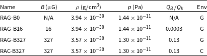


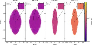

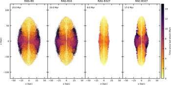


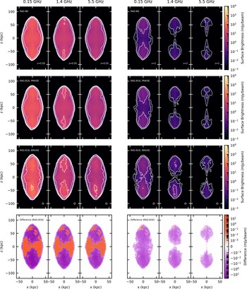


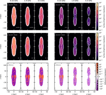


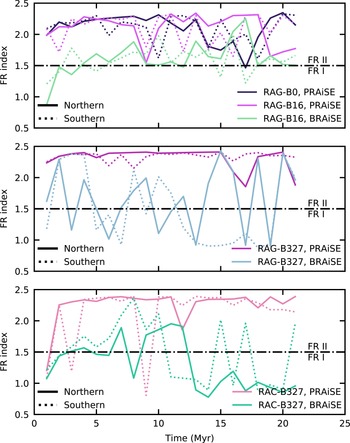


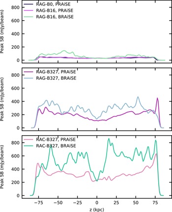


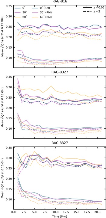


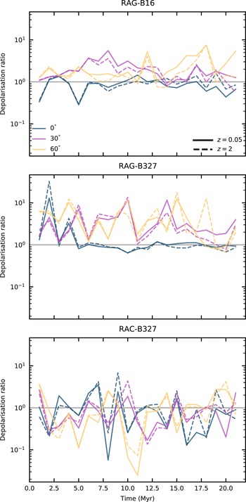


 Open access