

1. INTRODUCTION
High-precision (cm-level) relative positioning based on Global Navigation Satellite Systems (GNSS), such as the Global Positioning System (GPS), relies on integer resolution of the ambiguities in the carrier-phase data. Traditionally, short-baseline (usually <10 km) ambiguity resolution based on dual-frequency GPS phase and code data is feasible within very short time spans, even instantaneously, based on just a single observation epoch (Teunissen, Reference Teunissen1994; Corbett and Cross, Reference Corbett and Cross1995; and Teunissen et al., Reference Teunissen, de Jonge and Tiberius1997). This rapidity is due to the strength of the short-baseline model since it is based on the assumption that the differential atmospheric delays are so small that they can be neglected. For longer baselines (e.g. up to a few hundred km) one however has to deal with significant differential atmospheric delays, mainly due to the ionosphere. The simplest method is to add both ionospheric and tropospheric unknowns to the model and estimate them in the processing. Unfortunately, the dual-frequency GPS model – which is often referred to as the “ionosphere-float” model (Teunissen, Reference Teunissen1997b) then becomes too weak and integer ambiguity resolution needs a much longer (convergence) time to be successful. Alternatively, the widely used “ionosphere-free” combination of dual-frequency GPS data results in a very small wavelength for the estimable integer ambiguity of the combination (Teunissen and Odijk, Reference Teunissen and Odijk2003), implying that rapid ambiguity resolution cannot be performed.
The performance of integer ambiguity resolution for long baselines is likely to be improved, which is due to a number of developments. First, GPS is being modernized from a dual-frequency to a triple-frequency system. The new GPS Block IIF satellites, which have been launched since 2010, transmit the new L5 signal. Initial analysis has already demonstrated that the precision of the code of L5 is better than the current GPS signals (De Bakker et al., Reference De Bakker, Tiberius, van der Marel and van Bree2012). Second, the realization of additional constellations next to GPS may be beneficial for long-baseline integer ambiguity resolution. In addition to the revitalization of the Russian GLONASS, new GNSS have been developed, such as the European Galileo and the Chinese BeiDou systems. In this paper we will look into the performance of long-baseline ambiguity resolution which can be expected when GPS and Galileo data are combined. The combination of GPS with Galileo is very interesting because it is anticipated that the quality of the new Galileo code data will be good (Colomina et al., Reference Colomina, Miranda, Pares, Andreotti and Hill2011). The availability of precise code data is important for fast ambiguity resolution, since they largely govern the precision of the float ambiguity solution.
Since the Galileo constellation is still under development, in this article the performance of ambiguity resolution is predicted by means of the ambiguity success rate, which is evaluated based on the functional and stochastic assumptions of the ionosphere-float GPS+Galileo model, thus without the need to collect real data. Despite the fact that long-baseline ambiguity resolution based on only a single epoch of data will not be possible under a GPS+Galileo scenario (Tiberius et al., Reference Tiberius, Pany, Eissfeller, de Jong, Joosten and Verhagen2002), it is still of interest to quantify the reduction in (convergence) time of ambiguity resolution when combining both constellations. Previous studies have already provided insight into the time-to-fix for the GPS+Galileo ambiguities. Zhang et al. (Reference Zhang, Cannon, Julien and Alves2003) demonstrated (based on software simulations) that for a 50 km baseline triple-frequency GPS, about 70 s is needed to fix the integer ambiguities, while this is only about 35 s for triple-frequency Galileo, and for GPS+Galileo combined this is about 20 s. Comparable numbers for the time-to-fix can be found in Sauer et al. (Reference Sauer, Vollath and Amarillo2004) for triple-frequency GPS-only (67 s) vs. triple-frequency (60 s) Galileo-only ambiguity resolution for a 85 km baseline, based on a hardware simulation, although the final Galileo frequencies and GPS L5 frequency have not been used. Ambiguity success rate simulations based on GPS, Galileo and combined GPS+Galileo have been carried out by Verhagen et al. (Reference Verhagen, Teunissen and Odijk2007), but there the focus was on instantaneous (single-epoch) full ambiguity resolution, based on the ionosphere-weighted model, restricting the baseline length to 100 km. As compared to these older studies, the novelty of this article can be summarized as follows:
• The integrated GPS+Galileo model presented in this article parameterises the ionospheric delays as explicit unknowns as we do not form ionosphere-free combinations. This model applies to the general multi-frequency case and is therefore not restricted to dual- or triple-frequency cases.
• Partial ambiguity resolution is investigated as an alternative to full ambiguity resolution. With the availability of more satellites and more frequencies for combined GPS+Galileo, it may not always be necessary to resolve the complete vector of integer ambiguities, but instead only a subset of it. Partial ambiguity resolution for long GPS baselines has already been introduced by Teunissen et al. (Reference Teunissen, Joosten and Tiberius1999) and later also applied by Dai et al. (Reference Dai, Eslinger and Sharpe2007) and Takasu and Yasuda (Reference Takasu and Yasuda2010).
• In our simulations no linear combinations of multi-frequency GPS and Galileo ambiguities are formed a priori, in contrast to Zhang et al. (Reference Zhang, Cannon, Julien and Alves2003), in which wide-lane and extra wide-lane combinations are formed. In our case, the Least-Squares AMBiguity Decorrelation Adjustment (LAMBDA) method (Teunissen, Reference Teunissen1994) is used to determine the ambiguity (subset) combinations that are best resolvable. This has the additional advantage that the information content of the actual receiver-satellite geometry is also used in this process.
The remainder of this paper is presented as follows. Section 2 briefly reviews the theory of (partial) integer ambiguity resolution and the success rate. Section 3 then discusses the mathematical details of the model's underlying long-baseline ambiguity resolution and positioning. Results of ambiguity success rate simulations for various long-baseline models (GPS-only, Galileo-only and GPS+Galileo) are presented in Section 4. Finally, the work is concluded in Section 5.
2. (PARTIAL) INTEGER AMBIGUITY RESOLUTION
2.1. Solving the GNSS model
In a very general form, the GNSS (linearized) model of observation equations can be cast into the following framework:
 $$E(y) = A_1 a + A_2 b,\,{\rm with}\quad a \in {\opf Z}^n, \, b \in {\opf R}^q ; \quad D(y) = Q_y $$
where E(·) denotes the expectation operator, y the vector of observed-minus-computed observations, a the n-vector of integer ambiguities, b the q-vector of real-valued parameters (e.g. the baseline coordinates, ionospheric and tropospheric delays, etc.), A 1 and A 2 their respective partial design matrices, D(·) the dispersion operator, and Q y the variance-covariance matrix of the observables. Usually, this GNSS model is solved in three steps. In the first step the integer constraint on the ambiguities is ignored and using standard least squares the so-called float solution is obtained for all parameters, denoted as:
 $$\left[ {\matrix{{\hat a} \cr {\hat b} \cr}} \right];\quad \left[ {\matrix{ {Q_{\hat a}} & {Q_{\hat a\hat b}} \cr {Q_{\hat b\hat a}} & {Q_{\hat b}} \cr}} \right]$$
with â the float ambiguity solution, Q â its variance matrix,  $\hat b$ the float solution of the real-valued parameters and $Q_{\hat b} $ its variance matrix. The covariance matrix between the real-valued parameters and the ambiguities is denoted as $Q_{\hat b\hat a} $. The float ambiguity solution is in a next step input in the LAMBDA method to obtain the integer least-squares solution by means of decorrelation and search. Once the integer ambiguities have been resolved, the real-valued parameters are improved by conditioning them to the integer ambiguity solution. As a result, a very precise solution is obtained, governed by the phase precision.
2.2. The ambiguity success rate
The precision improvement of the fixed real-valued parameters with respect to their float counterparts is based on the assumption that the estimated integer solution, which we denote as ă, corresponds to the correct solution, denoted as a. This should always be inferred by means of integer validation techniques. A prerequisite to correct integer estimation is that the underlying model is strong enough and this can be verified by evaluating the ambiguity success rate, which is the probability of correct integer estimation. It can be computed once the integer estimator and float ambiguity variance matrix Q â are known. Hence, it can be used as a planning tool, without the need to collect and process real data, as done earlier by Jonkman et al. (Reference Jonkman, Teunissen, Joosten and Odijk2000) and Milbert (Reference Milbert2005).
In this contribution we will use the ambiguity success rate based on the integer bootstrapping estimator, for which an easy to evaluate closed-form expression is available, and which is lower bounding the success rate of the optimal integer least-squares estimator (Teunissen, Reference Teunissen1999):
 $$\matrix{ {P(\breve {a} = a) = P(\breve {z} = z)\; \geqslant \underbrace {\prod\limits_{i = 1}^n {\left[ {2{\rm \Phi} \left( {\displaystyle{1 \over {2\sigma _{\hat z_{i|I}}}}} \right) - 1} \right]}} _{\rm ASR}} \cr}, \quad {\rm with} \quad {\rm \Phi} (x) = \int_{ - \infty} ^x {\displaystyle{1 \over {\sqrt {2\pi}}}} \exp \left\{ { - \displaystyle{1 \over 2}v^2} \right\}dv$$
where the integer least-squares success rate is denoted as P(ă=a) or  $P(\breve {z} = z)$, where $\breve {z} $ and z denote the integer least-squares solution and correct solution based on the LAMBDA-decorrelated ambiguities. The function Φ(x) is the normal distribution function, and $\sigma _{\hat z_{i|I}}, $ with I={i+1,…, n}, denotes the standard deviation of the conditional ambiguities. These ‘conditional standard deviations’ equal the square roots of the elements of the diagonal matrix D, when an LTDL-decomposition of the decorrelated ambiguity variance matrix $Q_{\hat z} $ is applied. In the examples in this article this LAMBDA-decorrelation is always applied, since then the bootstrapped success rate is a very sharp lower bound to the integer least-squares success rate (Verhagen, Reference Verhagen2003). In this contribution the bootstrapped ambiguity success rate is referred to as “ASR”.
2.3. (Partial) integer ambiguity resolution
Some GNSS models may not be strong enough to resolve the full vector of integer ambiguities with a success rate that is high enough. For example, if a new satellite rises, it may take some time before its integer ambiguities can be resolved in a long-baseline model for which the differential ionospheric delays cannot be ignored. In that case it may be an alternative to resolve only a subset of 1⩽p⩽n ambiguities, for which the success rate equals at least a minimum required value, i.e.:
 $$\matrix{ {\prod\limits_{i = p}^n {\left[ {2{\rm \Phi} \left( {\displaystyle{1 \over {2\sigma _{\hat z_{i|I}}}}} \right) - 1} \right]} \; \geqslant \; P_0} \cr} $$
with P 0 the minimum required success rate (e.g. 0·999 or 0·99). This approach for partial ambiguity resolution (PAR) was first introduced in Teunissen et al. (Reference Teunissen, Joosten and Tiberius1999). The procedure to determine the subset of ambiguities is now as follows. One starts with the LAMBDA-decorrelated ambiguity with the highest precision, this is always the last ambiguity in the vector, i.e.  $\hat z_n $, and checks if the success rate is at least equal to P 0. If this is the case, one then continues with the conditional ambiguity $\hat z_{n - 1|n} $ and so on, until the success rate becomes too small. We then can split the decorrelated solution into a part that is not fixed and a part that is fixed:
 $$\underbrace {\left[ {\matrix{ {\hat z_{\,p - 1}} \cr {\hat z_{n - p + 1}} \cr}} \right]}_{\hat z}\; = \; \underbrace {\left[ {\matrix{ {Z_{\,p - 1}^T} \cr {Z_{n - p + 1}^T} \cr}} \right]}_{Z^T} \hat a$$
with  $\hat z_{\,p - 1} $ the (decorrelated) subset that is kept as real-valued parameters and $\hat z_{n - p + 1} $ the subset that is fixed to integers. The decorrelating Z-transformation matrix is denoted as Z=[Z p−1, Z n−p+1], for which holds that |Z|=±1. In Equation (5) the transposition (denoted as ·T) of this matrix is used. The partially fixed integer solution, denoted as $\breve {z} _{n - p + 1} $, is now obtained through the integer least-squares search of the LAMBDA method:
 $$\breve {z} _{n - p + 1} \; = \; S(\hat z_{n - p + 1} );\; \quad S:\; {\opf R}^{n - p + 1} \to {\rm} {\opf Z}^{n - p + 1} $$
with S(·) denoting the integer mapping function from the space of reals to the space of integers. The solution of the real-valued parameters of interest, conditioned on the partially fixed integer solution, is computed as follows:
 $$\eqalign{& \hat b_{|\breve {z} _{n - p + 1}} \; = \; \hat b - Q_{\hat b\hat z_{n - p + 1}} Q_{\hat z_{n - p + 1}} ^{ - 1} (\hat z_{n - p + 1} - \breve {z} _{n - p + 1} ); \cr & Q_{\hat b_{|\breve {z} _{n - p + 1}}} \; = \; Q_{\hat b} - Q_{\hat b\hat z_{n - p + 1}} Q_{\hat z_{n - p + 1}} ^{ - 1} Q_{\hat z_{n - p + 1} \hat b}} $$
with  $Q_{\hat z_{n - p + 1}} = Z_{n - p + 1}^T Q_{\hat a} Z_{n - p + 1} $, $Q_{\hat b\hat z_{n - p + 1}} = Q_{\hat b\hat a} Z_{n - p + 1} $ and $Q_{\hat z_{n - p + 1} \hat b} = Q_{\hat b\hat z_{n - p + 1}} ^T $. It is noted that if p=1, all ambiguities are fixed and partial corresponds to full ambiguity resolution.
2.4. (Partially-) fixed vs. float precision of the real-valued parameters
Provided that the success rates of full and partial fixing are sufficiently high, i.e.  $P(\breve {z} _n = z_n ) \approx 1$ and $P(\breve {z} _{n - p + 1} = z_{n - p + 1} ) \approx 1$, we can make the following ranking concerning the precision of the real-valued parameters (of interest, e.g. the baseline coordinates):
 $$Q_{\hat b_{|\hat z_n}} \leqslant Q_{\hat b_{|\hat z_{n - p + 1}}} \leqslant Q_{\hat b} $$
i.e. the precision of the partially-fixed real-valued solution is worse than that of the solution based on the fully fixed ambiguity vector, but still better than of the float solution. Depending on the application at hand, one has to decide whether the precision of the partially-fixed solution is sufficiently better than that of the float solution. If this is not the case, one may strengthen the model by including more epochs of data so as to fix more ambiguities in order to improve the partially-fixed real-valued solution.
3. THE ATMOSPHERE-FLOAT GNSS MODEL
For long baselines, instead of forming linear combinations of frequencies to eliminate the ionospheric delays, in this contribution ionospheric parameters are estimated together with the other parameters. Also, (residual) tropospheric delay parameters are estimated, in addition to the a priori correction of the observations for the tropospheric delays using a standard model (Saastamoinen, Reference Saastamoinen1972). In this section this so-called atmosphere-float observation model is derived, for a single constellation, as well as a dual constellation. In this atmosphere-float model it is assumed that the positions of the satellites have been calculated using precise orbits provided by the International GNSS Service (IGS; Dow et al., Reference Dow, Neilan and Rizos2009), and because of their high quality in relation to the length of the baseline (a few hundreds of kilometres), it is not expected that orbit errors impact on the relative receiver position.
3.1. Single constellation model
Suppose we have a single-baseline linearized model of multi-frequency GPS phase and code data, which can be denoted as follows, in double-differenced form for m satellites and for k epochs, making use of a compact Kronecker product notation, analogous to Odijk and Teunissen (Reference Odijk and Teunissen2008):
 $$\eqalign{E\left( {\left[ {\matrix{ \phi \cr p \cr}} \right]} \right) = & \; \left[ {\matrix{ {\left( {\matrix{ {e_f} \cr {e_f} \cr}} \right)\otimes \left( {\matrix{ {D_m^T G_1} \cr \vdots \cr {D_m^T G_k} \cr}} \right)\; \;} & {\left( {\matrix{ {\rm \Lambda} \cr 0 \cr}} \right) \otimes \left( {\matrix{ {I_{m - 1}} \cr \vdots \cr {I_{m - 1}} \cr}} \right)} &}} \right. \cr &\left. {{ {\left( {\matrix{ { - \mu} \cr \mu \cr}} \right)}{ \otimes \left( {\matrix{ {I_{m - 1}} & {} & {} \cr {} & \ddots & {} \cr {} & {} & {I_{m - 1}} \cr}} \right)} \cr}} \right]\left[ {\matrix{ g \cr a \cr \imath \cr}} \right] \cr D\left( {\left[ {\matrix{ \phi \cr p \cr}} \right]} \right) = & \; \left( {\matrix{ {C_\phi} & {} \cr {} & {C_p} \cr}} \right) \otimes 2\left( {\matrix{ {D_m^T W_1^{ - 1} D_m} & {} & {} \cr {} & \ddots & {} \cr {} & {} & {D_m^T W_k^{ - 1} D_m} \cr}} \right)} $$
 Here the vectors of observed-minus-computed dual-frequency phase and code double-differenced observables (expressed in length unit) are denoted as ϕ=(ϕ 1T,…,ϕ fT)T and p=(p 1T,…,p fT)T, respectively, for f frequencies, with f⩾2. Furthermore, we denote the f-vector with ones as e f=(1,…,1)T, the diagonal matrix with wavelengths as Λ=diag(λ 1,…,λ f), and the vector of ionospheric coefficients as μ=(μ 1,…,μ f)T, with μ f=(λ f/λ 1)2. The time-varying matrices G i account for the receiver-satellite line-of-sight vectors plus tropospheric mapping function and have dimension m×4, while the (m−1)×m-matrix D mT is the between-satellite difference matrix, i.e. D mT=[−e m−1,I m−1] with e m−1 a vector with ones at all entries and I m−1 the identity matrix, both of dimension m−1. The parameter vector consists first of all of the vector g=(cT, τ), which contains the 3D (incremental) coordinate vector c and the (relative) zenith tropospheric delay (ZTD) parameter τ. Other parameters are the vector of integer ambiguities, denoted as a=(a 1T,…,a fT)T and the vector of ionospheric delays, denoted as ı. Both ambiguity and ionospheric parameters are double differences. All parameters are expressed in length unit, except for the ambiguities, which are expressed in cycles. Note that in the notation of the real-valued parameters in Section 2 for this model it holds that b=(gT, ıT)T. The coordinates are assumed to be time-constant, which applies to stationary receivers. The ambiguities are constant in time as well, provided that the phase data are corrected for cycle slips. It is assumed that the (residual) ZTDs are time-constant as well, which is allowed considering that the time spans considered in this article are at most about 30 minutes (see Section 4). The ionospheric delays are assumed to be time-varying, without any dynamic model linking them in time. In the stochastic model C ϕ and C p denote the f×f cofactor matrices of the undifferenced phase and code observables, respectively, while D mTWi− 1D m accounts for the variances and covariances due to the differencing between satellites and the factor 2 is to account for the differencing between the two receivers forming the baseline. Through the diagonal matrix W i satellite dependent observation weighting can be applied to account for the reduced accuracy of the observations at lower elevations: W i=diag([q i1]2,…,[q im]2), with  $q_i^s = \sin {\epsilon} _i^s $ where the satellite's elevation is denoted as ${\epsilon} _i^s $.
3.2. Dual constellation model
Having data of a second constellation available, for both GNSSs we can set up a model of observation equations conforming to Equation (9) and solve each model for its parameters. However, the coordinate and ZTD parameters are system independent and thus common for both GNSSs. This is added as the following constraint to the systems of observation equations:
 $$g_{GPS} {\rm =} g_{GAL} {\rm =} g$$
if we denote the coordinate/ZTD vector for GPS as g GPS and the corresponding solution for Galileo as g GAL. This constraint can also be taken into account by combining the observables of both GNSSs into an integrated model of observation equations for which one common vector of coordinates+ZTD is parameterised.
4. SIMULATED AMBIGUITY SUCCESS RATES FOR A LONG BASELINE
This section presents results of the success rates of ambiguity resolution and precision of the coordinates for a fictitious long static baseline, where the receiver-satellite geometries of both GPS and Galileo are simulated for the full day of 13 May 2011, based on Yuma almanac data. The full GPS constellation is assumed to consist of 24 satellites and the full Galileo constellation of 27 satellites. The reference receiver is assumed to be located at −30o latitude and 115o longitude. The rover receiver is assumed at a distance of 250 km in the East direction, thus at the same latitude. The ASRs are predicted for a static baseline setup, in which the rover receiver is assumed not to be in motion. Figure 1 depicts the number of GPS and Galileo satellites that are tracked at the location of the reference receiver during the selected day.
Number of satellites as function of time of the day as used in the computations: GPS (blue), Galileo (red) and GPS+Galileo (black).

For both GPS and Galileo triple-frequency data are assumed to be collected above a cut-off elevation of 10o using high-grade geodetic receivers at both ends of the baseline. For these receivers the following values are assumed for the (undifferenced) standard deviations of the GPS and Galileo observations, in local zenith:
• For GPS:
○ L1: phase 3 mm; code 25 cm
○ L2: phase 3 mm; code 25 cm
○ L5: phase 2 mm; code 15 cm
• For Galileo:
○ E1: phase 3 mm; code 25 cm
○ E5a: phase 2 mm; code 15 cm
○ E5b: phase 2 mm; code 15 cm
For GPS it is assumed that the precision of the new L5 signal is better than that of the current L1 and L2 frequencies. For Galileo the precision of both E5a and E5b are assumed better than that of E1.
In all computations it is assumed that the integer ambiguities are correctly fixed if ASR⩾P 0=0·999, for both full as well as partial ambiguity resolution (FAR vs. PAR). In case of PAR, the time to fix the ambiguities is not only driven by the a priori set success rate, but additionally it is required that the partially-fixed coordinates are sufficiently accurate: the standard deviation of the position in East and North directions should be better than 2 cm, while the standard deviation in the Up direction is required to be smaller than 6 cm. This sub-decimetre precision requirement still necessitates the use of ambiguity resolution.
Since all computations are purely based on the assumptions in the model's design matrix and variance-covariance matrix, see Equation (9), we emphasize that it is not necessary to simulate the observations themselves or to put any assumption on the size of the ionospheric and tropospheric delays, as well as the satellite orbit errors.
4.1. GPS-only results
Table 1 shows the number of epochs that are on average needed for successful FAR and PAR during this day, based on GPS data only. To investigate the effect of a varying sampling interval on the mean number of epochs or Time-To-Fix-Ambiguities (TTFA), results are presented for two choices: a sampling interval (ΔT) of 10 s, as well as 30 s. From the table it can be seen that FAR based on traditional L1+L2 observations requires on average 96 epochs or 16 minutes of data based on 10 s sampling, and 64 epochs or 32 minutes based on 30 s sampling. With a longer sampling interval the required number of epochs is less, since the receiver-satellite geometry changes more from one epoch to the other, which is favourable for ambiguity resolution. The benefit of PAR is only limited here: the TTFA reduces to 14 minutes based on 10 s sampling and to 25 minutes based on 30 s sampling. Ambiguity resolution based on L1+L5 already requires less time, which is basically due to the better code precision of the L5 data. Slightly better performances can be expected using all three frequencies simultaneously: the mean TTFA is 11 minutes for FAR based on 10 s sampling and 20 minutes based on a sampling of 30 s.
GPS-only daily mean number of epochs (k) to fix the ambiguities and corresponding Time-To-Fix-Ambiguities (TTFA). For both FAR and PAR it is required that ASR ⩾0·999, while in addition for PAR the position standard deviations in North, East, Up are required to be better than 2, 2, 6 cm, respectively.

Figure 2 presents the GPS-only results in graphical form, for the 10-s sampling interval, for certain batches of data during the day. The left three graphs depict the ASR as well as the coordinate precision before and after FAR. For the sake of visualization, the 3D coordinate precision is compressed into a scalar value by taking the determinant of the float/fixed variance matrix and raising them to the power of 1/6 in order to obtain a ‘standard deviation-like’ value, i.e.  $|Q_{\hat c} |^{1/6} $ for the float coordinate precision and $|Q_{\hat c_{|\hat z_{n - p + 1}}} |^{1/6} $ for the (partially-) fixed coordinate precision. An important property of these determinants is that they also measure the volume of the position confidence ellipsoids. In the graphs the fixed coordinate precision is plotted from the moment the ASR is large enough (0·999) such that the ambiguities can be reliably fixed. At that epoch in the graphs there is a jump downwards, so as to mark the precision improvement due to ambiguity fixing. The fixed precision, based on FAR, at the epoch of fixing is at the level of a few millimetres and depicted in red at the right side of the right y-axis in each graph. The three graphs on the right side of the figure show the results based on PAR. In addition to the curves for the ASR and float/fixed coordinate precision, the PAR graphs depict a blue curve, which in a stepwise manner shows the percentage of ambiguities that are partially fixed. For example, for L1+L2 PAR fixes 17% of the ambiguities after the ASR criterion has just been met. However, at that point of time the criterion concerning the (partially) fixed coordinate precision is not yet met (it is still very close to the float precision at sub-metre level). Inspection of the LAMBDA-decorrelated Z-matrix reveals that the ambiguities that are first fixed by PAR are all wide-lane-like combinations. In the case of dual-frequency GPS the traditional wide lanes of L1 and L2 show up as the most precise ambiguity combinations, and this was already noted in Teunissen (Reference Teunissen1997a). In the modernized GPS case the L2-L5 wide lane (the so-called “extra” wide lane) shows up as the most precise ambiguity combination. Since these wide-lane combinations have a relatively long wavelength (Cocard et al., Reference Cocard, Bourgon, Kamali and Collins2008), they can be quickly fixed. Unfortunately, the fixing of these wide-lane combinations only results in a coordinate precision which is marginally better than the precision based on the float solution, see the Appendix, which further elaborates on this. Therefore, PAR requires more epochs to fix a larger subset of ambiguities (in addition to these wide lanes) in order to deliver the required coordinate precision. The length of this time thus determines the TTFA and number of ambiguities based on PAR. For the sake of completeness the blue curve in the graphs is continued until 100% of ambiguities are fixed, corresponding to the TTFA needed for FAR. The graphs also show that for GPS L1+L5 the coordinate precision criterion based on PAR is not met at all and therefore the TTFA corresponds to that of FAR.
GPS-only ambiguity success rates (ASR) and coordinate precision vs. number of epochs, for: L1+L2 (top), L1+L5 (middle) and L1+L2+L5 (bottom), for a data sampling interval of 10 s. The left graphs relate to FAR, while the right graphs relate to PAR, both based on the criterion that ASR ⩾0·999. The brown curve shows the ASR as a function of number of epochs within the batch, whilst the red curve depicts the float coordinate precision, and the green curve the (partially) fixed coordinate precision. Before this criterion is met, the fixed precision curve corresponds to its float counterpart. The blue curves on the right refer to the percentage of ambiguities that are (partially) fixed, i.e. 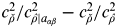 ${\textstyle{{n - p + 1} \over n}} \times 100\% $, with n the total number of ambiguities and where p equals the number of fixed ambiguities.
As an additional illustration to the above, consider a triple-frequency GPS example, in which at a certain epoch six satellites are tracked, such that there are n=3×(6−1)=15 double-differenced ambiguities to be resolved. Based on decorrelation of these ambiguities the success rate for FAR turns out to be about 0·05, which is much lower than the requirement of 0·999. Figure 3 (left) plots the (partial) success rate as function of p, i.e. the size of the subset of ambiguities that is fixed with PAR. Here the ordering of the ambiguities is such that the last ambiguity has the best precision and the first ambiguity the poorest precision. From the figure it follows that for a subset of the last 10 ambiguities in the vector (i.e. for p=6) the success rate is high enough such that the requirement of 0·999 is fulfilled; fixing more ambiguities would lower the success rate too much. It turns out that this subset of ten ambiguities corresponds to the wide-lane combinations: five “extra” wide lane combinations of L2 and L5, plus five traditional wide lanes of L1 and L2. Although the success rate is fulfilling the criterion, the resulting coordinate precision based on these ambiguity combinations is not high enough (only at sub-metre level). However, after a time span of about 15 minutes, the model has gained sufficient strength due to the change in receiver-satellite geometry, and the coordinate precision with PAR fulfils the required level (standard deviation below 2 cm for North and East and below 6 cm for Up). During this time, a new satellite has risen, extending the ambiguity vector to dimension n=3×(7−1)=18. Figure 3 (right) shows the success rate as a function of the size of the subset that can be fixed with PAR for this case. It can be seen that from p=4 the success rate is higher than 0·999; thus a subset of 15 ambiguities can be fixed. Comparing the ambiguity combinations that are partially fixed with those of 15 minutes before, reveals that they consist of the same L2-L5 and L1-L2 wide-lanes as could be fixed earlier, but now also the L2-L5 and L1-L2 wide lanes corresponding to the newly risen satellite show up in the subset. However, in addition to these wide lanes, as due to the increased strength of the model, the three L5 ambiguities can be fixed, and these are the ambiguities that actually contribute to the improvement in the precision of the coordinates.
Ambiguity success rate (ASR) as function of subset of 1⩽p⩽n ambiguities that is partially fixed, for the triple-frequency GPS case with: (left) six satellites, for which the partially-fixed coordinate standard deviations are (0·36, 0·85, 0·48) m for East-North-Up, and (right) seven satellites, 15 minutes later than the first example, for which the partially-fixed coordinate standard deviations are (0·01, 0·02, 0·04) m for East-North-Up. The ASR at p=1 corresponds to the success rate of FAR.
4.2. Galileo-only results
Similar to the GPS-only cases, Table 2 and Figure 4 present the results for the Galileo-only cases, restricted to the combinations E1+E5a and E1+E5a+E5b. It can be seen that the TTFAs are in the same order as for the GPS-only cases; for FAR as well as PAR. The shortest TTFA takes about 10 minutes for PAR based on E1+E5a+E5b and a sampling interval of 10 s.
Galileo-only ambiguity success rates (ASR) and coordinate precision vs. number of epochs, for: E1+E5a (top) and E1+E5a+E5b (bottom), for a data sampling interval of 10 s. The left graphs relate to FAR, while the right graphs relate to PAR, both based on the criterion that ASR ⩾0·999. See Figure 2 for an explanation of the different curves.
Galileo-only daily mean number of epochs (k) to fix the ambiguities and corresponding Time-To-Fix-Ambiguities (TTFA). For both FAR and PAR it is required that ASR ⩾0·999, while in addition for PAR the position standard deviations in North, East, Up are required to be better than 2, 2, 6 cm, respectively.

4.3. GPS+Galileo results
Table 3 and Figure 5 show the results when GPS and Galileo are combined. Two cases are analysed: the L1+L5 & E1+E5a case with two overlapping frequencies, and the L1+L2+L5 & E1+E5a+E5b case, which includes three frequencies from each system. From the results it follows that the combination of GPS+Galileo reduces the TTFA for FAR based on the 10 s sampling interval: from about 12–13 minutes in the single-system cases, to about seven minutes for L1+L5 & E1+E5a. In the case of L1+L2+L5 & E1+E5a+E5b the improvement is even better: from about 11–12 minutes in the single-constellation cases, to only two minutes in the combined case (based on 10 s sampling interval). When the PAR technique is used, the combination of GPS and Galileo benefits the TTFA for the presented cases. For the L1+L5 & E1+E5a case the TTFA varies between three minutes (10 s sampling) and seven minutes (30 s sampling), while theses times are 10–20 minutes for the single-constellation cases. The time required for PAR in the multi-frequency L1+L2+L5 & E1+E5a+E5b case is only in the order of one minute (10 s sampling) to two minutes (30 s sampling).
GPS+Galileo ambiguity success rates (ASR) and coordinate precision vs. number of epochs, for: L1+L5 & E1+E5a (top) and L1+L2+L5 & E1+E5a+E5b (bottom), for a data sampling interval of 10 s. The left graphs relate to FAR, while the right graphs relate to PAR, both based on the criterion that ASR ⩾0·999. See Figure 2 for an explanation of the different curves.
GPS+Galileo daily mean number of epochs (k) to fix the ambiguities and corresponding Time-To-Fix-Ambiguities (TTFA). For both FAR and PAR it is required that ASR ⩾0·999, while in addition for PAR the position standard deviations in North, East, Up are required to be better than 2, 2, 6 cm, respectively.

5. CONCLUSIONS
This article has investigated the expected performance of integer ambiguity resolution for precise long-baseline (a few hundred km) positioning based on an anticipated combination of a modernized GPS and a full Galileo constellation. The ambiguity resolution performance is thereby measured in terms of the ambiguity success rate, computed from the variance-covariance matrix of the float ambiguities estimated with the atmosphere-float GPS+Galileo model. The following conclusions can be drawn from the simulation studies described in this article:
• The combination of triple-frequency data of both systems, i.e. GPS L1+L2+L5 and Galileo E1+E5a+E5b, results in significantly shorter times to fix the ambiguities compared to the ambiguity resolution times that can be expected for single-constellation observations.
• Resolving a subset of ambiguities, instead of the full vector, i.e. partial ambiguity resolution, is especially beneficial in shortening the times-to-fix-ambiguities in a combined GPS+Galileo setup. The gain of partial fixing for a single-constellation model is only marginal, since a relatively long time is needed to resolve those ambiguity combinations that are needed to realise a significant improvement in coordinate precision.
• With partial ambiguity resolution in a combined GPS+Galileo case, it has been demonstrated that for a 250 km baseline it takes only one to two minutes to fix the ambiguities, compared to 15–25 minutes in the dual-frequency L1+L2 GPS-only case.
We finally emphasize that all results presented in this paper are predictions, i.e. we did not use real observational data to arrive at the above conclusions. When real dual-constellational GPS+Galileo data become available, more work is required on analysing the performance of the proposed method in difficult ionospheric conditions, as there may be issues such as, for example, divergence of the filter state vector or long convergence time of the position solution (Richtert and El-Sheimy, Reference Richtert and El-Sheimy2005). In addition, more studying is required to understand the benefits and negative aspects of ionospheric delay estimation compared to using the ionosphere-free combinations. More results of GPS+Galileo ambiguity success rate predictions, for short as well as long baselines, can be found in Arora (Reference Arora2012).
ACKNOWLEDGEMENTS
This work is done in the context of the Australian Space Research Program (ASRP) project “Platform Technologies for Space, Atmosphere and Climate” and the Positioning Program Project 1.01 “New carrier phase processing strategies for achieving precise and reliable multi-satellite, multi-frequency GNSS/RNSS positioning in Australia” of the Cooperative Research Centre for Spatial Information (CRC-SI). The third author is the recipient of an Australian Research Council (ARC) Federation Fellowship (project number FF0883188). All this support is gratefully acknowledged.
APPENDIX – IMPACT OF FIXING OF COMBINATIONS OF GPS L1 AND L2 AMBIGUITIES ON THE COORDINATE PRECISION
Unfortunately, fixing of certain ambiguity combinations, such as the traditional wide lane in case of dual-frequency GPS, results in a coordinate precision that is only marginally better than the precision based on the float solution, i.e. without ambiguity fixing. This can be seen as follows. The variance matrix of the coordinate and ZTD parameters can be given as the following analytical expressions, for the atmosphere-float model with all ambiguities float (denoted using the “hat” symbol on top of the vectors) and all ambiguities fixed (denoted using the “check” symbol) (Odijk and Teunissen, Reference Odijk and Teunissen2008):
 $$\eqalign{Q_{\hat g} = & c_{\breve {\rho}} ^2 \left[ {\displaystyle{{c_{\breve {\rho}} ^2} \over {c_{\hat \rho} ^2}} \sum\limits_{i = 1}^k {G_i^T} P_m G_i + \left( {1 - \displaystyle{{c_{\breve {\rho}} ^2} \over {c_{\hat \rho} ^2}}} \right)\sum\limits_{i = 1}^k ( G_i - \bar G)^T P_m (G_i - \bar G)} \right]^{ - 1} \cr Q_{\breve {g}} = & c_{\breve {\rho}} ^2 \left[ {\sum\limits_{i = 1}^k {G_i^T} P_m G_i} \right]^{ - 1}} $$
with  $c_{\hat \rho} $ and $c_{\breve {\rho}} $ the square roots of the ambiguity-float and ambiguity-fixed variance factors of the receiver-satellite range parameters that can be estimated using the geometry-free version of our atmosphere-float model (Odijk, Reference Odijk2008). In Odijk and Teunissen (Reference Odijk and Teunissen2008) it is demonstrated that the term $c_{\hat \rho} $ is governed by the precision of the code observations and is therefore large, while the term $c_{\breve {\rho}} $ is governed by the phase precision and therefore about a factor 100 smaller. Since both expressions in Equation (A1) have the factor $c_{\breve {\rho}} ^2 $ in common, the difference between float and fixed coordinate precision is due to the differences between the terms within the “inverse brackets”. In case of the fixed variance matrix, this term is an epoch-wise summation of 4×4 matrices that are a function of the receiver-satellite geometry, i.e. G iTPmGi, with P m denoting a satellite-dependent projector matrix (Odijk and Teunissen, Reference Odijk and Teunissen2008) and G i the matrices containing the line-of-sight vectors plus the tropospheric mapping coefficients, see Equation (9). In case of the float variance matrix the term inside the inverse brackets looks a bit more complicated. Firstly, it consists of a part that appears in the fixed variance matrix as well, however now scaled by $c_{\breve {\rho}} ^2 /c_{\hat \rho} ^2 $, i.e. the ratio of fixed and float variance factors, but this ratio is very small, about 10−4 in practice. The second part is an epoch-wise summation again involving the receiver-satellite geometry matrices G i, but now differenced with respect to $\bar G = \sum\nolimits_{i = 1}^k {G_i} $, which is the averaged geometry matrix over all epochs. This means that if the observation time span is short, this summation term is relatively small compared to the first summation, since the receiver-satellite geometry only changes slowly, and the individual geometry matrices will therefore not differ much from their time-averaged counterpart. In addition to this, the factor before the summation term, i.e. $1 - c_{\breve {\rho}} ^2 /c_{\hat \rho} ^2 $, is very close to one in practice. Thus, the float variance matrix is governed by the second part within the inverse brackets in Equation (A1) and therefore relatively poor as compared to the fixed variance matrix.
In case of partial fixing of a subset of L1 and L2 ambiguity combinations, i.e. a αβ=αa 1+βa 2, with α and β scalar integers, it can be shown that the variance matrix of the coordinates+ZTD conditioned on these partially-fixed ambiguities can be given as:
 $$Q_{\hat g|a_{\alpha \beta}} = c_{\breve {\rho}} ^2 \left[ {\displaystyle{{c_{\breve {\rho}} ^2} \over {c_{\hat \rho |a_{\alpha \beta}} ^2}} \sum\limits_{i = 1}^k {G_i^T} P_m G_i + \left( {1 - \displaystyle{{c_{\breve {\rho}} ^2} \over {c_{\hat \rho |a_{\alpha \beta}} ^2}}} \right)\sum\limits_{i = 1}^k ( G_i - \bar G)^T P_m (G_i - \bar G)} \right]^{ - 1} $$
Note that this expression is similar to the expression of the float coordinate variance matrix in Equation (A1), except that  $c_{\hat \rho} ^2 $ is replaced by $c_{\hat \rho |a_{\alpha \beta}} ^2 $, which is the variance factor of the ranges in the geometry-free model, but now based on a fixing of the subset of ambiguities only. Table A1 shows for several choices of α and β the difference between the variance ratios appearing in the float and partially-fixed variance matrix expressions, i.e. $c_{\breve {\rho}} ^2 /c_{\hat \rho |a_{\alpha \beta}} ^2 - c_{\breve {\rho}} ^2 /c_{\hat \rho} ^2 $, which should lie somewhere between 0 and 1. It can be seen that for the traditional wide lane, i.e. α=1 and β=−1, this additional term is 0·000014, close to zero, which means that $Q_{\hat g|a_{\alpha \beta}} \approx Q_{\hat g} $, implying that fixing of this wide lane hardly improves the partially-fixed coordinate precision as compared to the float precision. This also holds for other wide-lane like combinations, such as α=−3 and β=4, and α=−2 and β=3. It even holds when only the L1 or L2 ambiguities are fixed, i.e. α=1 and β=0 and α=0 and β=1. On the other hand, there are also combinations for which the additional term is close to 1, e.g. α=9 and β=−7, or α=77 and β=−60 (this latter combination corresponds to the well-known ionosphere-free combination). For these combinations it holds that $Q_{\hat g|a_{\alpha \beta}} \approx Q_{\breve {g}} $ and thus fixing of such combinations has a large effect on the coordinate precision. However, despite their benefit for the coordinate precision these ambiguity combinations cannot be quickly fixed, due to their very short wavelengths. On the other hand, the combinations that can be quickly fixed due to their long wavelength, such as the traditional wide lane, hardly have an effect on improving the coordinate precision.
GPS dual-frequency ambiguity combinations aαβ=αa 1+βa 2, their virtual wavelength λ αβ and their effect on the coordinate precision measured through factor $c_{\breve {\rho}} ^2 /c_{\hat \rho |a_{\alpha \beta}} ^2 - c_{\breve {\rho}} ^2 /c_{\hat \rho} ^2 $.


