2.1. Data

The PST–SMP field dataset consists of 83 side-by-side field measurements that were conducted in the Swiss Alps around Davos on 19 days between 1 March 2010 and 3 March 2015. On each of these days, SMP measurements and PST experiments were performed no further than 0.3 m from each other and adjacent to a snow pit at a distance of <5 m. The manual snow profile (CAA, 2007) included manual density measurements with a 100 cm³ density cutter. The SMP measurements were conducted along a contour line of the slope and snow columns were prepared for PTV analysis of PST experiments – each one close to an SMP measurement. The PTV data are part of a larger, recently published dataset (van Herwijnen and others, Reference van Herwijnen, Gaume, Bair, Reuter, Birkeland and Schweizer2016). The SMP data were partly used earlier by Reuter and others (Reference Reuter, van Herwijnen, Veitinger and Schweizer2015b). Here we show the overlapping data, i.e. the cases with SMP measurements and adjacent PST experiments, which allow deriving snow properties from every measurement. The snow properties derived from this dataset are for snow layers with a thickness of ~1 up to several centimetres.

The SMP–μCT laboratory dataset includes SMP measurements and μCT measurements that were previously presented by Riche and Schneebeli (Reference Riche and Schneebeli2013) and Proksch and others (Reference Proksch, Löwe and Schneebeli2015). The dataset consists of 27 natural snow samples and nature identical snow samples produced with the ‘snow maker’ (Schleef and others, Reference Schleef, Jaggi, Löwe and Schneebeli2014). From the centre of the snow samples, one μCT sample (≤0.5 cm³) was extracted and up to four SMP measurements were taken around the location of the μCT sample allowing direct comparison. A sketch of the original measurement setup is provided by Proksch and others (Reference Proksch, Löwe and Schneebeli2015, Fig. 2a therein). The snow structural properties derived from these data correspond to cubes of several 0.1 cm³.

To compare the snow properties measured with different methods, we analyzed the correlations and report the coefficient of determination R ². In the case of linear regressions, we also provide the p-values of regression coefficients to describe the significance of the regression slope (assuming a level of significance p = 0.05). The measurement uncertainty of SMP-derived density was assessed with the RMSE in relation to the reference measurement. Moreover, we provide the mean absolute error (MAE), which weighs individual errors equally, and provides together with the RMSE a measure for the deviation among individual errors.

2.2. Miro-computed tomography and finite element modelling

μCT allows to reconstruct the full 3-D microstructure of snow (Schneebeli and Sokratov, Reference Schneebeli and Sokratov2004), which can be used in a subsequent finite element analysis to determine linear elastic properties (e.g. Schneebeli, Reference Schneebeli2004; Srivastava and others, Reference Srivastava, Mahajan, Satyawali and Kumar2010; Köchle and Schneebeli, Reference Köchle and Schneebeli2014; Wautier and others, Reference Wautier, Geindreau and Flin2015). The μCT scans were performed with different nominal resolutions (voxel size) between (10 μm)³ for new snow samples and (18 μm)³ for depth hoar. The size of the scanned volume was selected manually to ensure representative elementary volumes, which ranged between (5.9 mm)³ for new snow and (7.1 mm)³ for depth hoar. The attenuation image (grey scale image) resulting from each scan was filtered using a Gaussian filter (σ = 1 voxel, kernel half-width = 2 voxel) following Kerbrat and others (Reference Kerbrat, Pinzer, Huthwelker, Gäggeler, Ammann and Schneebeli2008) and then segmented into a binary image. The threshold for segmentation was constant for each sample and determined visually.

From the binary image, snow density (ρ _CT) was determined from the ice volume fraction and the density of ice. By standard means of a voxel-based finite element solution of the equations of elasticity for composites (Garboczi, Reference Garboczi1998) the elastic stiffness tensor was computed. The same numerical method has been previously used in Srivastava and others (Reference Srivastava, Chandel, Mahajan and Pankaj2016) or Gerling and others (Reference Gerling, van Herwijnen and Löwe2017). In the present analysis, we used a bulk modulus of 8.9 GPa and a shear modulus of 3.52 GPa, corresponding to polycrystalline ice at −16°C (Petrenko and Whitworth, Reference Petrenko and Whitworth1999). The components of the elastic stiffness tensor E of the snow samples were then determined by averaging stresses and strains over the sample volume according to Garboczi (Reference Garboczi1998). We consider a Cartesian coordinate system with the two axes (1,  0,  0) and (0,  1,  0) spanning up the horizontal plane and the third axis perpendicular (0,  0,  1) and in the opposite direction of gravity. For the present analysis, we assumed snow to be a transversely isotropic material (Shertzer and others, Reference Shertzer, Adams and Schneebeli2011) and calculated E ₁₁ = E ₂₂, E ₃₃, ν ₁₂ = ν ₂₁, ν ₁₃ and ν ₃₁ from three FE simulations. In each simulation, a uniaxial strain of 0.001 was prescribed in one of the three coordinate directions. Solving a system of linear equations, the elastic moduli E ₁₁ = E ₂₂, E ₃₃ for a transversely isotropic material were recovered.

From the penetration resistance signal of the SMP, however, we do not obtain directional material properties. In fact, the deformation measured at the tip of the device during snow penetration is a superposition of the deformation of many individual elements (Johnson and Schneebeli, Reference Johnson and Schneebeli1999). Hence, directional differences are obscured and with the current signal interpretation, only a single mean estimate of the modulus is retrieved from the SMP penetration resistance signal. In contrast, with FE simulations of μCT images, the components of the modulus can be computed and the directional differences of the material properties of snow become apparent. In the following, we show how to derive a modulus that relates to the deformation at the penetrometer tip. For comparison with SMP measurements, we will translate the transverse isotropic material properties obtained from the finite element analysis of μCT images into an isotropic-equivalent modulus. In other words, this modulus refers to an isotropic material showing the same strain vector as the transversely isotropic material and is obtained after setting equal the compliance forms of the stress-strain relations. Solutions only exist for particular stress states, two of which we describe in the following.

Under the assumption, the stress has a horizontal and a vertical component and the relation between them is a, i.e. σ = (aσ ₃₃,  0,  σ ₃₃,  0,  0,  0) in Voigt notation, an isotropic equivalent modulus E _iso can be derived for an orthotropic material:

(1)$$ E_{\rm iso} = {\displaystyle{E_{11}E_{33} (1 - a^2)} \over {E_{33} - a^{2} E_{11} + aE_{33}\nu_{13} - aE_{11}\nu_{31}}}. $$

In the case of the SMP, the ratio between the vertical and horizontal stresses a can be expressed by the SMP cone half angle (30°) and the friction coefficient between ice and steel (Johnson and Schneebeli, Reference Johnson and Schneebeli1999) yielding 0.65 with a friction coefficient of 0.05. As we consider snow as a transversely isotropic material with the axis of symmetry along (0,  0,  1) we know, E ₃₃ν ₁₃ = E ₁₁ν ₃₁ and Eqn 1 simplifies to:

(2)$$ E_{\rm iso} = {\displaystyle{E_{11} E_{33} (1-a^2)} \over {E_{33} - a^2 E_{11}}}. $$

Alternatively, if the stress is confined to the two dimensions not including the axis of symmetry, i.e. σ = (bσ ₂₂, σ ₂₂,  0,  0,  0) in Voigt notation with b the ratio between the horizontal components, the isotropic equivalent modulus for a transversely isotropic material (i.e. E ₁₁ = E ₂₂) with the axis of symmetry along (0,  0,  1) equals the elastic modulus of the isotropic plane:

(3)$$ E_{\rm iso} = {\displaystyle{E_{11} E_{22} (1-b^2)} \over {E_{22} - b^2 E_{11}}} = E_{11}=E_{22}. $$

Both assumptions have been used to describe the stress state during penetration in the past. Johnson and Schneebeli (Reference Johnson and Schneebeli1999) described the stress exerted by the SMP tip with a vertical and one horizontal component. More recently, Ruiz and others (Reference Ruiz, Capelli, van Herwijnen, Schneebeli and Or2017) used the penetration model by Bishop and others (Reference Bishop, Hill and Mott1945) who described cone penetration with radial and circumferential stresses only. Hence, in this case, the stress is confined to the isotropic plane of a snow sample with transversely isotropic material symmetry. In the following, we will consider both cases as it is presently not clear, which better describes snow penetration with the SMP. We thus refer in the following to either Eqn 3, when the stress is confined to the isotropic plane or to Eqn 2, when the stress is not confined to the isotropic plane.

2.3. Snow micro-penetrometry

The SMP contains a high-resolution force sensor driven into the snow cover at constant speed which measures the penetration resistance of snow layers. By interpreting fluctuations of the penetration resistance as a Poisson shot noise process as proposed by Löwe and van Herwijnen (Reference Löwe and van Herwijnen2012), the SMP signal can be described by three microstructural parameters, namely the rupture force f, the deflection at rupture δ and the structural element size L. The parameters were calculated over a moving window w of 2.5 mm with 50 % overlap and then averaged over layers which were manually identified. This setting was sufficient to capture even the thinnest layers in our dataset, i.e. the window size was small enough to resolve weak layers of several millimetres. Given the SMP measurement resolution, dealing with even thinner layers seems feasible, if the finer window and evaluation step sizes are selected. By visual inspection signals of lower quality were excluded following the procedure outlined in Pielmeier and Marshall (Reference Pielmeier and Marshall2009). Signal processing included correcting for penetration resistance offset determined from the noise level measured in the air signal prior to snow penetration. For the comparison with the μCT-derived snow properties, we averaged the SMP-derived microstructural properties, as up to four SMP measurements were available around one μCT sample. We used SMP devices of version 2, among others the device SMP 21.

2.3.1. Density

It has been shown that snow density is related to median penetration resistance $\widetilde {F}$ (Proksch and others, Reference Proksch, Löwe and Schneebeli2015; Kaur and Satyawali, Reference Kaur and Satyawali2017). Proksch and others (Reference Proksch, Löwe and Schneebeli2015) modified the relation by Pielmeier (Reference Pielmeier2003) by including the structural element length L to account for differences in snow microstructure. We used the formulation presented by Proksch and others (Reference Proksch, Löwe and Schneebeli2015):

(4)$$ \rho_{{\rm SMP}} = a_1 + a_2 \ln(\widetilde{F}) + a_3 \ln(\widetilde{F}) L + a_4 L, $$

and their original coefficients a ₁ = 420.47, a ₂ = 102.47, a ₃ = −121150, and a ₄ = −169960 for $\widetilde {F}$ in N, L in m and ρ in kg m⁻³.

2.3.2. Elastic modulus

Based on foam theory, Johnson and Schneebeli (Reference Johnson and Schneebeli1999) suggested calculating an elastic modulus from the microstructural parameters f, δ and L according to

(5)$$ E_{{\rm macro}} = {\displaystyle{\,f} \over {\delta L}} {\displaystyle {\delta} \over {L}}. $$

where the first term is the microscale modulus and the second term (δ/L) accounts for the number of grains in contact with the SMP tip. Marshall and Johnson (Reference Marshall and Johnson2009) applied their formulation to penetration resistance signals of natural snow samples and obtained values for the micro-scale modulus in the range of 0.1–1 MPa i.e. about one order of magnitude lower than corresponding literature values such as provided in Mellor (Reference Mellor1975). Also, in more recent comparisons SMP-derived microscale moduli were similarly low and not clearly related to those determined from acoustic wave propagation (Capelli and others, Reference Capelli, Kapil, Reiweger, Or and Schweizer2016; Gerling and others, Reference Gerling, van Herwijnen and Löwe2017). These discrepancies were suggested to be partly due to a missing assumption for the particle shape in the SMP analysis (Marshall and Johnson, Reference Marshall and Johnson2009).

In addition to Eqn 5, we suggest an alternative formulation for an effective modulus that can be derived from the microstructural parameters f, δ and L. To this end, based on dimensional arguments, i.e. considering a deformation energy per volume, the elastic modulus can alternatively be described as:

(6)$$ E_{{\rm SMP}} = a_5 {\displaystyle {\,f \delta} \over {L^3}} {\displaystyle {\delta} \over {L}}. $$

In other words, a single rupture event is assumed to release an energy proportional to the product fδ, which increases with increasing modulus. Scaling by the structural element volume (L ³) a microscale modulus is recovered. Again, the microscale modulus is multiplied by ${\displaystyle {\delta } \over {L}}$ to derive the macroscale modulus. The above formulation of the microscale modulus, i.e. the first part of Eqn 6 coincides with the formulation suggested by Johnson and Schneebeli (Reference Johnson and Schneebeli1999) for the macroscale strength. We will compare the two formulations Eqns 5 and 6 and determine the coefficient a ₅ in the Results section from comparisons with μCT measurements and literature data.

In the FE simulations of μCT samples, the linear elastic response of the material to a given strain is calculated, whereas the SMP-derived effective modulus may still contain contributions of non-elastic deformation – despite the relatively high strain rate. In fact, the strain rate during SMP penetration can be estimated to ${\dot \epsilon } \approx 100\,{\rm s}^{-1}$ assuming a typical deflection at rupture δ = 10⁻⁵ m, a typical structural element size L = 10⁻⁴ m and the penetration speed of the SMP (20 × 10⁻³ m s⁻¹). Hence, snow grains in front of the SMP tip are likely to fail after very little deformation, i.e. in a brittle manner. Nonetheless, from the SMP signal analysis, we do not obtain a truely elastic modulus, but rather an effective modulus. This is partly, because we do not account for geometric scaling due to indenter size (Huang and Lee, Reference Huang and Lee2013). Moreover, we neglect possible snow compaction near the SMP tip (van Herwijnen, Reference van Herwijnen2013; LeBaron and others, Reference LeBaron, Miller and van Herwijnen2014) which leads to an overestimation of the deformation energy in the initial phase of deformation. Hence, with Eqn 6 we calculated a deformation energy fδ containing not only elastic contributions and eventually obtain values lower than the true elastic modulus. This said we refer to the SMP-derived effective modulus from Eqn 6 by E _SMP.

2.3.3. Slab modulus

To compare with the PTV-derived effective moduli, an elastic modulus of the slab consisting of several layers was calculated using a FE model with the SMP-derived layer properties as input (Reuter and Schweizer, Reference Reuter and Schweizer2018). The properties include snow layer thickness, density (from Eqn 4) and effective elastic modulus E _SMP (from Eqn 6). The geometry and loading conditions are similar to a PST and the model was previously used by van Herwijnen and others (Reference van Herwijnen, Gaume, Bair, Reuter, Birkeland and Schweizer2016). The base of the slab has rigid support on one side and is unsupported along a short crack on the other side. Increasing the length of this crack the change in mechanical energy was determined. Fitting pairs of crack length and mechanical energy with a beam equation (Heierli, Reference Heierli2008), we obtained the SMP-derived elastic modulus of the slab, which corresponds to the modulus of a uniform slab showing the same displacement as the layered slab. This modulus is termed SMP-derived elastic modulus of the slab or just SMP-derived slab modulus $E_{{\rm SMP}}^{{\rm slab}}$ (cf. Table 3).

Table 3. Overview of measured snow properties (rows) and measurement techniques (columns). Orange cells correspond to the SMP–μCT dataset, blue cells to the PST–SMP dataset

2.3.4. Specific fracture energy

The specific fracture energy (w _f,SMP) was determined by integrating the penetration force over the moving windows of width w and searching the window within the weak layer (WL) with the lowest value (Reuter and others, Reference Reuter, Schweizer and van Herwijnen2015a):

(7)$$ w_{{\rm f},{\rm SMP}} = {\rm min}_{\rm WL} \int_{-{w}/{2}}^{+{w}/{2}} F {\rm d}z. $$

In other words, the derivation of the fracture energy is based on the average penetration resistance, since the integral of the penetration resistance across a window of 2.5 mm can be expressed as the average of the measured SMP penetration resistance across this window times the window size. Under the assumption of elastic-brittle rupture events, the first cumulant of the shot noise process, i.e. the average of the measured penetration resistance, equals fδ/L ³. Hence, our alternative formulation to estimate the elastic modulus (Eqn 6) is as well based on the average SMP penetration resistance. This may seem paradoxical, but both mechanical properties are strongly related to material strength. As will be shown below, such SMP-derived estimates are useful to estimate the elastic modulus and the fracture energy of snow.

2.4. Propagation saw test and particle tracking

All PST experiments had similar dimensions (cross-slope width: 0.3 m, up-slope length: 1.2–2.2 m) and had slope normal, rather than vertical, column ends following recommendations and procedures of van Herwijnen and others (Reference van Herwijnen, Gaume, Bair, Reuter, Birkeland and Schweizer2016). A crack was introduced into the weak layer in up-slope direction with a 2 mm thick snow saw until a self-propagating crack started at a certain cut length, the critical cut length r _c. Numerous black markers were inserted in the snow above and below the weak layer and experiments were recorded with a video camera fixed on a tripod. Displacements were derived with PTV from all markers in the slab until the critical crack length was reached. The mechanical energy was calculated according to van Herwijnen and others (Reference van Herwijnen, Gaume, Bair, Reuter, Birkeland and Schweizer2016) from the product of snow density, thickness and average measured displacement of each row of makers. Snow layer densities and thicknesses were available from an adjacent manual snow profile. From the obtained pairs of mechanical energy and corresponding crack length the effective modulus of the snow slab ($E_{{\rm PTV}}^{{\rm slab}}$) was obtained by fitting an adjusted analytical expression for the mechanical strain energy provided by Heierli (Reference Heierli2008).

Based on finite element simulations, van Herwijnen and others (Reference van Herwijnen, Gaume, Bair, Reuter, Birkeland and Schweizer2016) showed that the analytical energy formulation does not fully describe the influences of slope angle and the ratio of crack length to slab thickness. For typical values of slope angle and slab thickness encountered in field experiments, a correction factor is required to obtain an adjusted mechanical energy. We applied the corrections described by van Herwijnen and others (Reference van Herwijnen, Gaume, Bair, Reuter, Birkeland and Schweizer2016). Values of the mechanical energy measured in those field experiments likely overestimate deformation due to non-elastic contributions (van Herwijnen and others, Reference van Herwijnen, Gaume, Bair, Reuter, Birkeland and Schweizer2016). The strain rate during PST experiments was estimated by van Herwijnen and others (Reference van Herwijnen, Gaume, Bair, Reuter, Birkeland and Schweizer2016) to between ${\dot \epsilon } = 6 \times 10^{-5}$ and 2 × 10⁻² s⁻¹ with a mean of 10⁻³ s⁻¹, i.e. in the range of the ductile-to-brittle transition for snow failure (Narita, Reference Narita1980; Schweizer, Reference Schweizer1998; Reiweger and Schweizer, Reference Reiweger and Schweizer2010). The PTV-method does, therefore, not provide a truly elastic modulus, but rather an effective modulus, which we call PTV-derived effective modulus of the slab $E_{{\rm PTV}}^{{\rm slab}}$.

The specific fracture energy of the weak layer (w _f,PTV) was calculated as the first derivative of the mechanical strain energy with respect to the critical crack length, which includes the previously derived effective modulus. The specific fracture energy could thus only be derived if crack propagation occurred to the end of the column (43 out of 83 experiments).

3.1. Density

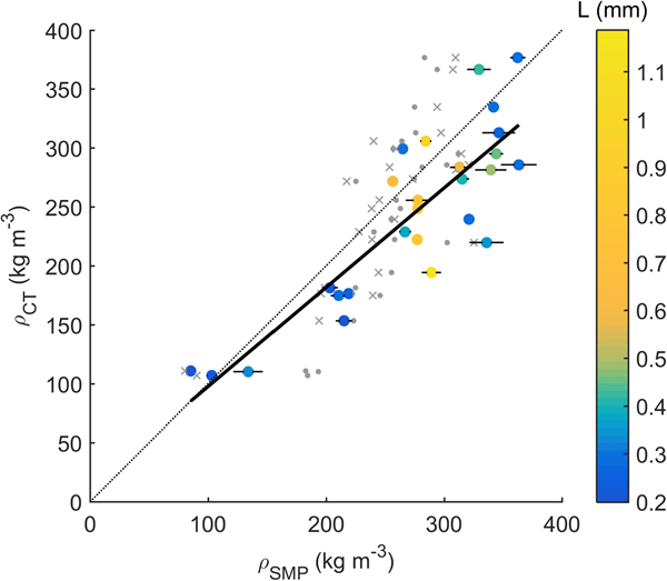
Snow densities derived from the SMP signal (Eqn 4) were clearly related to those obtained from the μCT (R ² = 0.74, p _slope < 0.001; Fig. 1). The SMP-derived density was somewhat overestimated, in particular, for higher densities (≥200 kg m⁻³). The uncertainty of the SMP-derived density as indicated by error bars in Fig. 1 were determined from side-by-side measurements with the SMP in the same snow sample (up to four per sample). Averaging the standard deviation of those side-by-side measurements yielded a RMSE of 9 kg m⁻³. The deviation between the two measurement methods could not be explained by the structural element length (L) (Fig. 1).

Fig. 1. μCT- and SMP-derived snow density with least squares fit (solid line) and 1:1 line (dotted line) for 27 snow samples of the SMP-μCT dataset (full coloured circles). Error bars indicate standard deviation from side-by-side SMP measurements. Data cover a broad range of different snow types indicated by the structural element size L (colour bar). Dots show the values obtained with the model of Kaur and Satyawali (Reference Kaur and Satyawali2017). Crosses show the values obtained after recalibrating the model of Proksch and others (Reference Proksch, Löwe and Schneebeli2015) to the presented data.

Sources of the uncertainty of μCT-derived snow density are in part related to the segmentation process (the SMP-CT dataset from Riche and Schneebeli (Reference Riche and Schneebeli2013) and Proksch and others (Reference Proksch, Löwe and Schneebeli2015) depend on) to obtain binary images and the measurement resolution (Hagenmuller and others, Reference Hagenmuller, Matzl, Chambon and Schneebeli2016), which was chosen according to the snow structure. Proksch and others (Reference Proksch, Rutter, Fierz and Schneebeli2016) reported an agreement between volumetric measurements obtained with density cutters and μCT measurements of 5–9%. Assuming μCT as the more accurate measurement method and hence considering it as a reference, the accuracy of density prediction from SMP-derived parameters was estimated to RMSE = 49 kg m⁻³ and MAE = 41 kg m⁻³. The observed RMSE is somewhat higher than that reported in Proksch and others (Reference Proksch, Löwe and Schneebeli2015) (30 kg m⁻³), although we used the same parameterization. Their fitting model is based on Alpine, Arctic and Antarctic data and dominated by the polar samples. Our data only include Alpine samples and are actually a subset of the data presented by Proksch and others (Reference Proksch, Löwe and Schneebeli2015). Recalibrating the model of Proksch and others (Reference Proksch, Löwe and Schneebeli2015) to our data subset, however, did not substantially change the correlation (R ² = 0.74). Applying the purely penetration resistance (F) based model of Kaur and Satyawali (Reference Kaur and Satyawali2017) to our data, yielded a lower correlation (R ² = 0.63). Obviously, microstructural information is required to enhance the parametrization of snow density. Apart from the structural element size, other parameters may be useful. During snow sintering experiments, van Herwijnen and Miller (Reference van Herwijnen and Miller2013) found an increase of measured penetration resistance with time related to an increase in bond-to-grain ratio, while snow density remained essentially constant. To correctly reflect this, a microstructural property compensating the increase of the average penetration resistance F would be required – apart from L, which rather refers to the average distance between breaking microstructural elements.

The reported agreement between μCT- and SMP-derived density is based on the parameterization of Proksch and others (Reference Proksch, Löwe and Schneebeli2015). As electronic components and software have changed in more recent versions of the SMP, data derived with different devices will differ. Hence, to reproduce the presented agreement a calibration specific to the SMP device is required to obtain the fitting coefficients for the parameterizations based on the microstructural parameters.

3.2. Elastic modulus

The isotropic equivalent elastic modulus derived from μCT images with the finite element method and Eqn 3 ranged between 5 and 258 MPa. The elastic modulus increased with increasing density (full circles in Fig. 2, R ² = 0.87).

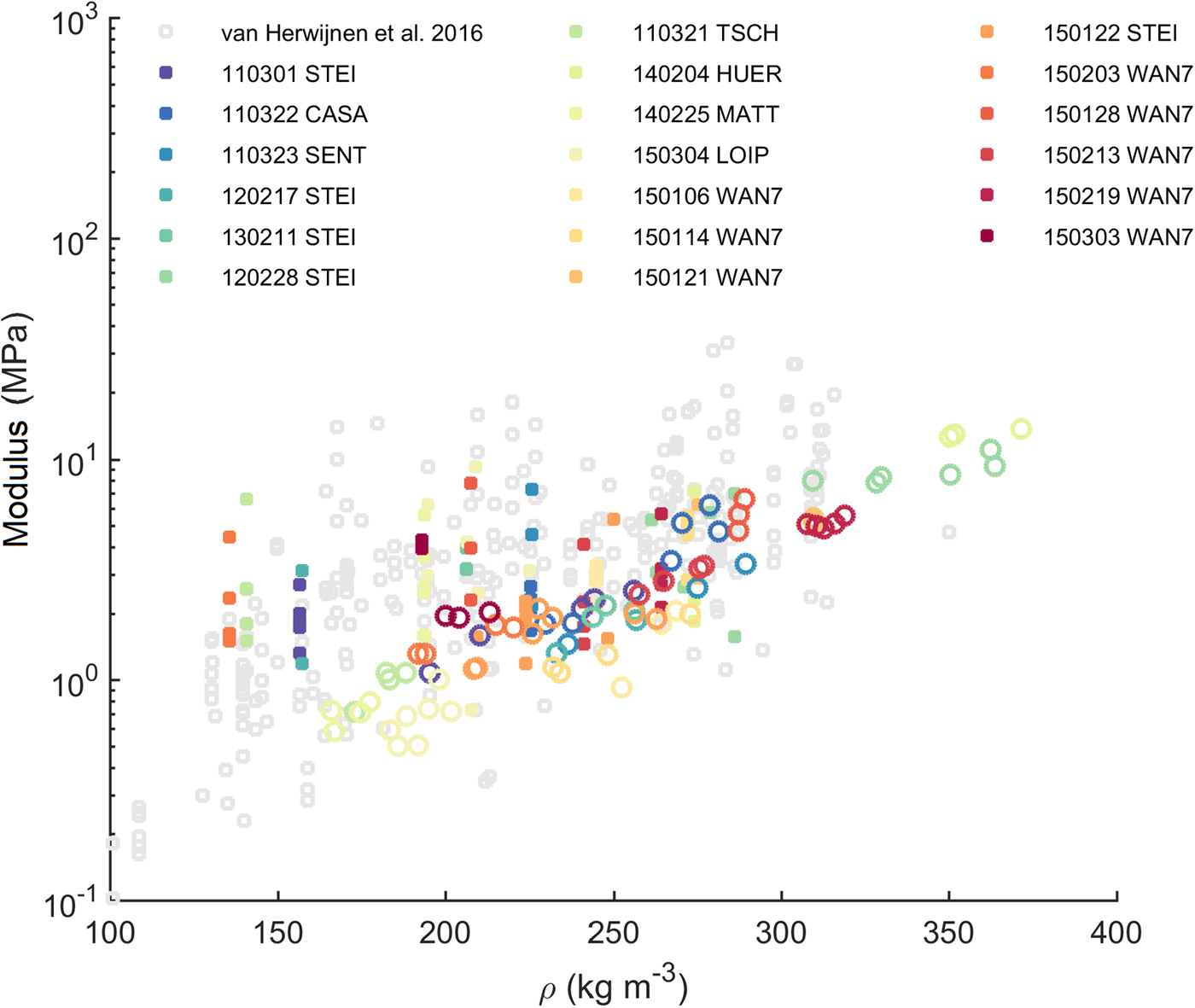
Fig. 2. SMP-μCT dataset: Isotropic equivalent elastic modulus computed from μCT imaging (full circles, Eqn 3) and effective modulus computed from SMP signals (open circles, Eqn 6) versus μCT-derived density for 27 snow samples. Colour bar indicates structural element size L derived from SMP signals as in Figure 1. Also shown, empirical relations of Köchle and Schneebeli (Reference Köchle and Schneebeli2014) by dotted lines, of Sigrist and others (Reference Sigrist, Schweizer, Schindler and Dual2006) by dash-dotted line, of Scapozza (Reference Scapozza2004) by dashed line and of van Herwijnen and others (Reference van Herwijnen, Gaume, Bair, Reuter, Birkeland and Schweizer2016) by full line.

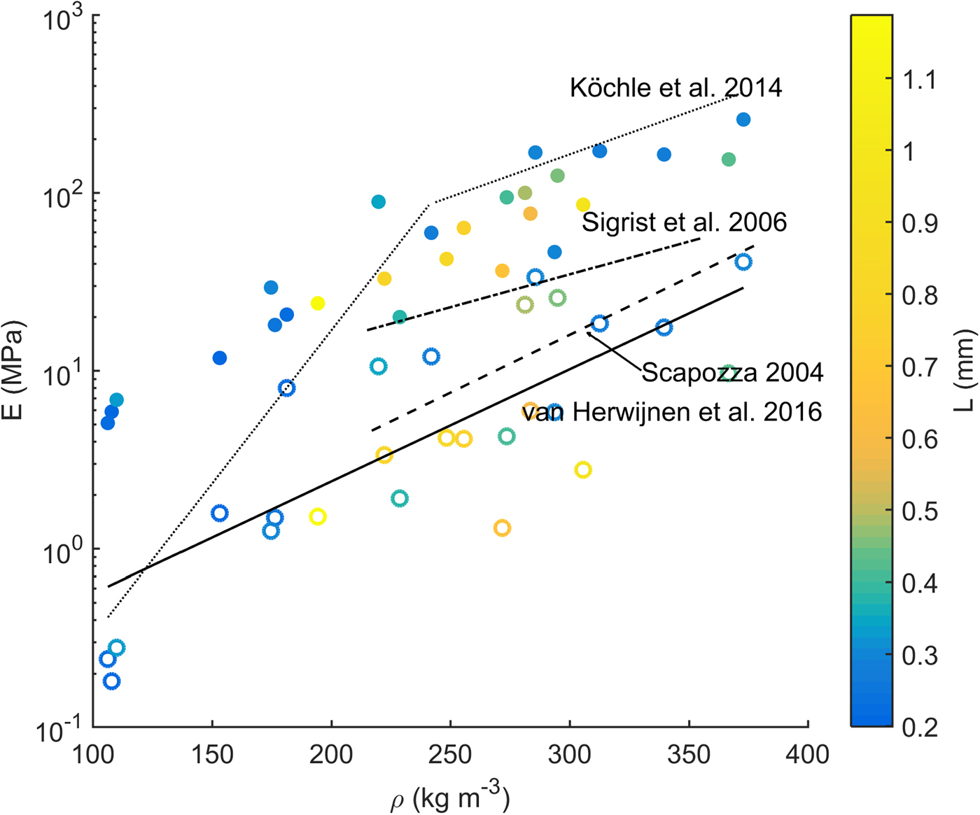
The μCT-derived values of the elastic modulus were comparable to values modelled by Schneebeli (Reference Schneebeli2004) for a sample of sifted snow with a density of 234 kg m⁻³ undergoing “temperature-gradient” metamorphism. During that process the modulus decreased from 226 to 62 MPa within 6 days. In Figure 2, the parameterizations covering the ranges 100–250 and 250–460 kg m⁻³ reported by Köchle and Schneebeli (Reference Köchle and Schneebeli2014) describe large parts of our μCT-derived values of the elastic modulus, except for low densities. The parameterization presented by Sigrist and others (Reference Sigrist, Schweizer, Schindler and Dual2006) based on cyclic loading experiments at high strain rates of about ~2.7 × 10⁻²s⁻¹ are the experimental values closest to μCT-derived values. Scapozza (Reference Scapozza2004) calculated the modulus from the stress increase observed at small deformations (ε = 0.125%) in quasistatic uniaxial compression tests. The parameterization with density, he proposed yields lower values of the modulus and a stronger increase with density (Table 4). The differences compared with the FE results of the modulus are likely related to the rather low strain rates in his experiments ranging between 10⁻⁶ s⁻¹ and 10⁻³ s⁻¹. van Herwijnen and others (Reference van Herwijnen, Gaume, Bair, Reuter, Birkeland and Schweizer2016) derived an effective modulus by PTV of the (layered) snow slab during propagation saw tests. Those values represent among the presented data the ones obtained at the lowest strain rate of about ${\dot \epsilon } = 10^{-3}\,{\rm s}^{-1}$ similar to the ones by Scapozza (Reference Scapozza2004) and presumably for the highest strain.

Table 4. Fit parameters p ₁ and p ₂ for exponential fit models of the elastic modulus E and density ρ: E = p ₁ · exp (p ₂ · ρ) and coefficient of determination R ².

For the SMP-μCT dataset μCT-derived density and for the PST-SMP dataset values measured with a density cutter were used. Subscripts CT, SMP and PTV indicate μCT, SMP- and PTV-derived values, respectively. The superscript ‘slab’ refers to an effective modulus accounting for the slab layering. Also parameterizations from previous studies shown in Fig. 2 are listed: Scapozza (Reference Scapozza2004) (Sc), Sigrist (Reference Sigrist2006) (Si) and Köchle and Schneebeli (Reference Köchle and Schneebeli2014)(KS < 250, KS > 250), for densities below and above 250 kg m⁻³, respectively. The data of van Herwijnen and others (Reference van Herwijnen, Gaume, Bair, Reuter, Birkeland and Schweizer2016) (vH) were fitted with an exponential model.

We also present the effective modulus calculated from SMP measurements performed adjacent to the samples used for the μCT scans in Figure 2 (open circles). A coefficient a ₅ of 880 (Eqn 6) was determined to match the data of Scapozza (Reference Scapozza2004) (R ² = 0.75) and was used to graph the data. The SMP-derived values ranged from 0.18 to 41 MPa and increased with density. Also the scatter increased with density yielding R ² = 0.66. For a particular density, the scatter may partly be related to differences in structural element length L (compare blue and yellow open circles in Fig. 2). However, measurement uncertainties and possible temperature effects we did not measure cause the large part of the observed variations of modulus in the graph with density.

The formulation suggested by Johnson and Schneebeli (Reference Johnson and Schneebeli1999) (Eqn 5) yielded a lower coefficient of determination (R ² = 0.53), more scatter and a decreasing trend of the modulus with densities above 300 kg m⁻³ (not shown). With the presented, alternative formulation (Eqn 6, R ² = 0.66) the increase of the SMP-derived effective modulus with density was in the range of the parameterizations presented by Sigrist and others (Reference Sigrist, Schweizer, Schindler and Dual2006), Scapozza (Reference Scapozza2004) and van Herwijnen and others (Reference van Herwijnen, Gaume, Bair, Reuter, Birkeland and Schweizer2016) (see Table 4). Note that the coefficient a ₅ for the SMP-derived effective modulus (Eqn 6) was estimated to fit the laboratory measurements of Scapozza (Reference Scapozza2004), since these data are numerous and cover a wide range of densities (Table 1). A calibration to the data of van Herwijnen and others (Reference van Herwijnen, Gaume, Bair, Reuter, Birkeland and Schweizer2016) is not straightforward due to different scales between the slab modulus obtained with the PTV method and the SMP-derived modulus for a single snow layer.

The SMP-derived values exhibited more scatter than FE model results of μCT images (cf. R ² in Table 4), probably due to measurement uncertainties. Moreover, for both, SMP- and μCT-derived values, the scatter was larger for densities above about 200 kg m⁻³. This was expected, as density alone cannot completely describe the complex snow structure (e.g. Shapiro and others, Reference Shapiro, Johnson, Sturm and Blaisdell1997; Schneebeli, Reference Schneebeli2004; Löwe and others, Reference Löwe, Riche and Schneebeli2013). Our low-density snow rather consisted of decomposed and fragmented precipitation particles. At higher densities ≳ 200 kg m⁻³, on the contrary, our snow samples showed a more diverse snow microstructure and a much broader range with different mechanical behaviour (cf. Srivastava and others, Reference Srivastava, Chandel, Mahajan and Pankaj2016).

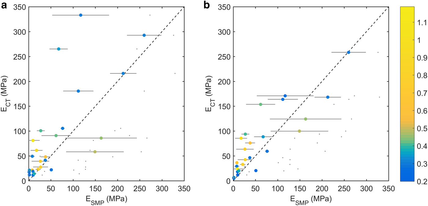
Figure 3 compares elastic moduli derived from μCT images and SMP signals of the SMP–μCT lab dataset. Assuming the stress was not in the isotropic plane (Eqn 2), the correlation between μCT- and SMP-derived elastic moduli was fair but significant (R ² = 0.52, p _slope < 0.01). Alternatively, assuming that the stress is confined to the isotropic plane (Eqn 3), as suggested by Ruiz and others (Reference Ruiz, Capelli, van Herwijnen, Schneebeli and Or2017), the correlation was stronger and significant (R ² = 0.76, p _slope < 0.01). The SMP effective modulus was derived from Eqn 6 with a coefficient a ₅ = 5600, which we had determined from a linear regression with the isotropic equivalent modulus from μCT images assuming the stress to be confined to the isotropic plane. Employing the density parametrization reported by Köchle and Schneebeli (Reference Köchle and Schneebeli2014) with SMP-derived snow density yielded a similar R ² = 0.79 when graphed with μCT-derived modulus from Eqn 3, i.e. assuming the stress was in the isotropic plane. Whereas the μCT-derived elastic modulus refers to an average volume of ≈ (5 mm)³, the corresponding SMP-derived values were averaged on a signal of length >1 cm. Error bars show the standard deviation determined from repeated SMP measurements around the μCT sample. The error bars provide an estimate for the errors due to inhomogeneities in the snow sample that affect this comparison. Also, errors due to the procedure to derive the modulus from SMP measurements are included, such as errors in signal inversion or the applied formulation of the elastic modulus. The linear regression analysis indicated that stronger deviations were more often observed in samples with large snow structures (L > 0.5 mm).

Fig. 3. SMP-derived modulus is shown with μCT-derived elastic modulus under the assumption (a) that the stress is not confined to the isotropic plane, i.e. derived from Eqn 2 or (b) that the stress is confined to the isotropic plane, i.e. derived from Eqn 3. Colour bar indicates structural element size L derived from SMP signals. Error bars show standard deviation from repeated SMP measurements. Also shown by grey dots are elastic modulus derived from SMP-derived density with the relation of Köchle and Schneebeli (Reference Köchle and Schneebeli2014) versus μCT-derived elastic modulus. 1:1 line dashed. N = 27.

The uncertainty involved with μCT imaging depends on segmentation thresholds and measurement resolution, as pointed out by Hagenmuller and others (Reference Hagenmuller, Matzl, Chambon and Schneebeli2016). Uncertainties of the SMP-derived elastic modulus are partly related to the structural parameters f, L and δ which are derived from the SMP signal. Directly computing the elastic modulus from the SMP parameters yielded a similar accuracy as computing the density from the SMP parameters and using a density parametrization of the elastic modulus (e.g. Köchle and Schneebeli, Reference Köchle and Schneebeli2014). With the similar accuracy of either approach, it seems the accuracy is limited by the presently used interpretation of snow micro-penetrometry. Concerning the elastic modulus, Srivastava and others (Reference Srivastava, Chandel, Mahajan and Pankaj2016) showed that with fabric-elasticity relations the derivation of the modulus based on μCT-measured snow structure could be enhanced. Moreover, SMP-derived signal characteristics such as correlation length and fractal dimension have the potential to describe snow structure (Satyawali and Schneebeli, Reference Satyawali and Schneebeli2010), which could be used in a statistical model to predict mechanical properties. So far, however, our interpretation of SMP penetration resistance allows us to derive a parameter set containing the rupture force f, the structural element length L and the deflection at rupture δ. Hence, to include further microstructural parameters into parameterizations, we need to advance the current interpretation of snow penetration or possibly derive additional parameters.

3.3. Slab modulus

From SMP measurements and PTV analysis, we obtained elastic moduli of the slab for the PST-SMP field dataset (Fig. 4). With the PTV method, some stratigraphic information is implicitly preserved, resulting in an effective slab modulus. To compare with SMP-derived moduli, we calculated the elastic modulus of the slab with a FE model, simulating the bending behaviour of a beam similar to the PST. PTV- and SMP-derived values of the slab modulus showed both an increase with snow density. PTV-derived values of the effective modulus showed more scatter than SMP-derived values (Table 4, cf. R²). From Figure 4 it becomes apparent that our PST-SMP dataset is a somewhat biased subset of the larger dataset of van Herwijnen and others (Reference van Herwijnen, Gaume, Bair, Reuter, Birkeland and Schweizer2016) who found a clearer relation with density (R² = 0.29).

Fig. 4. PST-SMP dataset: Effective slab modulus computed from SMP signals and FE modelling (open circles) and PTV analysis (full squares) versus SMP-derived snow density. Colours indicate different field sites. Grey open squares represent the entire dataset of van Herwijnen and others (Reference van Herwijnen, Gaume, Bair, Reuter, Birkeland and Schweizer2016).

With the PTV and the SMP method, we obtained lower values compared to the μCT-derived elastic modulus (cf. Fig. 2 and 4). As strain rates during PST experiments are relatively low, i.e. ${\dot \epsilon } \approx 10^{-3}\,{\rm s}^{-1}$ (van Herwijnen and others, Reference van Herwijnen, Gaume, Bair, Reuter, Birkeland and Schweizer2016), we anticipated that effective moduli derived with the PTV analysis would be low, and certainly lower than the true elastic modulus. On the contrary, effective moduli derived from the SMP signals are determined at high strain rates (${\dot \epsilon } \approx 100\,{\rm s}^{-1}$), but may still include some contribution of non-elastic deformation due to possible snow compaction at the tip. In Figure 4 SMP-derived values coincide with the lower values of the PTV-derived moduli. This, however, is rather due to the chosen calibration (coefficient a ₅ in Eqn 6). Calibrating SMP-derived properties is necessary to account for geometric scaling because the microstructural properties determined from the SMP depend on the indenter, i.e. its size and shape (Huang and Lee, 2013). We decided to calibrate the SMP data to the laboratory measurements of Scapozza (Reference Scapozza2004) since they cover a broad range of densities, despite the rather low values of strain rate during his experiments.

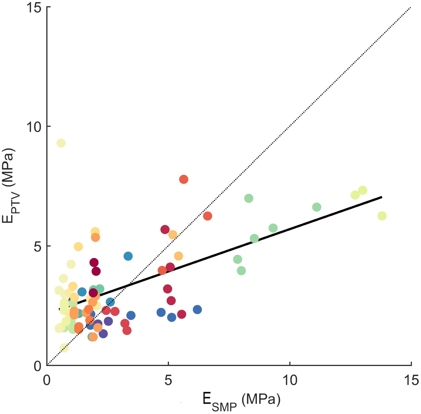
Figure 5 shows the direct comparison between PTV- and SMP-derived effective moduli from adjacent field experiments. Relating PTV- and SMP-derived values yielded a rather weak correlation (R ² = 0.36, p _slope < 0.01). This relation does not include the origin (0,0). Due to different strain rates and possible time-dependent deformation during the PST, a constant term in the regression may be needed to describe this relationship.

Fig. 5. PTV-derived versus SMP-derived elastic moduli of the slab. Colours indicate field sites with same legend as in Figure 6. Black line represents linear regression. N = 83.

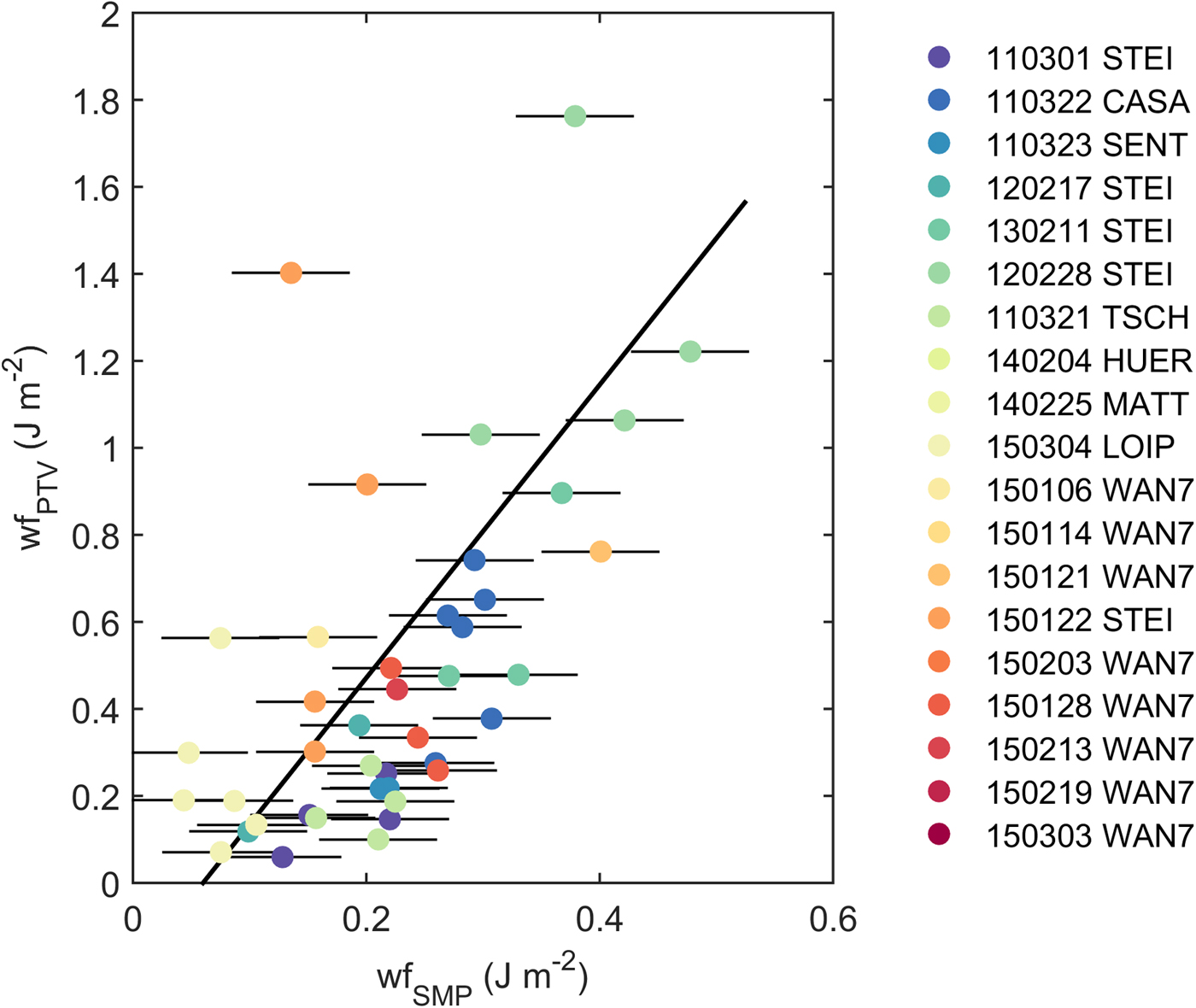
Fig. 6. Weak layer fracture energy derived with PTV analysis and from SMP signals including errorbars; colours indicate different field days and sites. One outlying PTV-derived value (w _f = 3 J m⁻²) excluded. N = 43.

With the PTV method an elastic modulus of the slab was determined for a bending snow column of ≤0.3 m³. From the SMP, we first calculated the elastic modulus (Eqn 6) and then computed a slab modulus using a FE model accounting for slab layering. This allowed comparing values derived from the two methods. After calibration the SMP-derived values of the slab modulus were in a similar range as the PTV-derived values. As shown in Figure 4 the subset of data we use is not representative of the entire dataset presented by van Herwijnen and others (Reference van Herwijnen, Gaume, Bair, Reuter, Birkeland and Schweizer2016). At low densities below $\lesssim \!\!200\,{\rm kg}\,{\rm m}^{-3}$ the data subset is biased towards higher moduli and at higher densities towards lower moduli. As only for this subset SMP measurements were available and in addition, PTV measurements naturally have an uncertainty of ~25%, the direct comparison with the limited data yielded a rather weak correlation. That said, uncertainties such as from snow density measurements likely play a less important role than the uncertainties from marker location tracking during PTV analysis.

3.4. Fracture energy

The specific fracture energy, the crucial weak layer property in view of crack propagation, describes the amount of energy needed to expand a crack over a given distance in the weak layer and form two new crack surfaces. The specific fracture energy derived from the SMP signal was related to the fracture energy derived from PST experiments with PTV (R ² = 0.40, p _slope < 0.001; Fig. 6). PTV-derived values were generally higher by a factor of 3.5 than SMP-derived values of w _f.

In contrast to PTV-derived moduli (Fig. 4 and 5), the fracture energy was only determined for those PST experiments where the crack propagated to the end of the column (43 of 83 cases). The error estimation was based on the repeated SMP measurements in the snow samples of the SMP–μCT dataset. From these samples, we estimated the variance of side-by-side penetration resistance measurements. As the derivation of the fracture energy is based on penetration resistance (Eqn 7), the uncertainty can thus be estimated by propagating the uncertainty of the measured penetration resistance. PTV-derived values were similar to those reported by Schweizer and others (Reference Schweizer, van Herwijnen and Reuter2011) (w _f = 1.3 ± 0.8 J m⁻²), who modelled the specific fracture energy with finite element simulations with effective moduli from SMP microstructural parameters derived after Marshall and Johnson (Reference Marshall and Johnson2009). In general, PTV-derived values overestimated the specific fracture energy as they are higher than literature values for ice; for example Schulson and Duval (Reference Schulson and Duval2009, p. 206) estimated w _f ≈ 0.32 J m⁻². As discussed in van Herwijnen and others (Reference van Herwijnen, Gaume, Bair, Reuter, Birkeland and Schweizer2016), the high values of fracture energy obtained with the PTV method suggest that a substantial fraction of the potential energy of the slab is dissipated during PSTs. Accounting for visco-plastic effects in the slab and in the weak layer is likely required to obtain more realistic values. Lower values of fracture energy w _f = (0.07 ± 0.02) J m⁻² were obtained by Sigrist and Schweizer (Reference Sigrist and Schweizer2007), who used a FE model with calibrated SMP-derived values of the effective modulus (Sigrist and others, Reference Sigrist, Schweizer, Schindler and Dual2006). Schweizer and others (Reference Schweizer, van Herwijnen and Reuter2011) discussed the importance of the choice of the modulus for these methods. Some methods, however, offer a way to determine the fracture energy and are independent of the modulus – and the measurement uncertainties involved. LeBaron and Miller (Reference LeBaron and Miller2014) presented a method based on μCT reconstructions of snow samples and calculated the critical energy release rate along the minimum cut surface (Hagenmuller and others, Reference Hagenmuller, Theile and Schneebeli2014b). Another approach circumventing assumptions in particular for the modulus, was presented by McClung (Reference McClung2015). He demonstrated that the specific fracture energy may be obtained from field measurements based on the ‘shear band model’ originally presented by Palmer and Rice (Reference Palmer and Rice1973). For his avalanche crown dataset he obtained values of w _f between 0.08 and 0.36 J m⁻² and similarly for a large dataset of 591 PSTs he reported values between 0.04 and 0.1 J m⁻². These two methods, namely the μCT-based and ‘shear band model’-based method, may allow calibrating SMP-derived values of the fracture energy independent of the modulus. So far, however, we did not calibrate SMP-derived values. Although the relationship between SMP- and PTV-derived values provides confidence in the SMP-derived property, calibrating with the PST–SMP dataset would shift the SMP-derived fracture energy towards unrealistically high values.