

1 INTRODUCTION
Extreme quantiles of unobserved individual heterogeneity (UIH) are of interest in the analysis of economic panel data and in meta-analysis. UIH includes heterogeneous coefficients, treatment effects, and other latent variables. For example, in the setting of Combes et al. (Reference Combes, Duranton, Gobillon, Puga and Roux2012), one might seek to estimate the lowest level of firm-specific productivity compatible with firm survival—the zeroth quantile of the productivity distribution among surviving firms.Footnote 1
However, inference on extreme quantiles is challenging as UIH is not directly observed—only noisy estimates derived from individual time series, studies, or clustered data are available. It is not a priori clear when such estimates yield useful information about the quantiles of interest. Unlike means, extreme quantiles do not benefit from noise “averaging out.” Moreover, estimation noise is often correlated with true UIH due to dependence between UIH and covariates used in estimation (e.g., Heckman, Reference Heckman2001; Browning and Carro, Reference Browning and Carro2007, Reference Browning and Carro2010), further complicating inference.
This article develops a methodology for inference on extreme quantiles of UIH using noisy estimates and establishes sharp conditions under which such estimates are informative. The key requirement is pointwise asymptotic tail equivalence (TE)—the tails of the noisy estimates’ distribution must converge in a certain weak pointwise sense to the tails of the latent UIH distribution. We construct confidence intervals (CIs) and hypothesis tests using self-normalizing ratios of extreme or intermediate order statistics and derive extreme and intermediate value theorems (IVTs) for noisy estimates.
Our inference methods rely on two asymptotic approximations: extreme order and intermediate order. Extreme order methods exploit ratios of the highest order statistics, and we show that the limiting distributions of these ratios can be estimated via subsampling or simulation. Intermediate order methods use ratios of statistics that are asymptotically in the tail but not the most extreme. We construct a ratio statistic that is asymptotically standard normal. This ratio requires no tuning parameters, in contrast to conventional intermediate order approaches (de Haan and Ferreira, Reference de Haan and Ferreira2006, Chap. 3). Our framework complements Jochmans and Weidner (Reference Jochmans and Weidner2024), who develop central order approximation methods for central quantiles of UIH.
We show that inference is valid if and only if TE holds, under minimal assumptions on the marginal distributions of UIH and estimation noise. The result allows for complex dependence structures between noise and true UIH, an important feature in non-experimental settings (Heckman, Reference Heckman2001; Browning and Carro, Reference Browning and Carro2007, Reference Browning and Carro2010).
For a broad class of distributions, we derive sufficient conditions for TE in terms of rates on the cross-sectional and individual sample sizes N and T. These conditions require standard moment or normality assumptions on the noise and a lower bound on the EV index. If the true UIH distribution has an infinite tail, TE holds under mild restrictions. For instance, if the noise has at least eight finite moments, inference remains valid provided $N/T^4 \to 0$
, matching the central quantile inference condition in Jochmans and Weidner (Reference Jochmans and Weidner2024). If the noise is Gaussian, N may grow almost exponentially relative to T. In contrast, rate conditions are stricter for distributions with finite endpoints, depending on the relative heaviness of UIH and noise tails.
$N/T^4 \to 0$
, matching the central quantile inference condition in Jochmans and Weidner (Reference Jochmans and Weidner2024). If the noise is Gaussian, N may grow almost exponentially relative to T. In contrast, rate conditions are stricter for distributions with finite endpoints, depending on the relative heaviness of UIH and noise tails.
We propose a rule of thumb for choosing inference methods. Broadly, the rule depends on N and the quantile of interest. For smaller N, extreme order methods are preferable for tail quantiles. In larger samples, one may also use the simpler intermediate order methods.
Our simulation studies show that if rate conditions hold, our methods offer favorable coverage properties in the tails. The rate conditions are important, and their failure may lead to distorted inference. We also show that our rule of thumb for method choice performs well.
We illustrate our methodology with an application to firm productivity in denser and less dense areas in the setting of Combes et al. (Reference Combes, Duranton, Gobillon, Puga and Roux2012). Our analysis addresses two key aspects of their study. First, we examine firm selection, which is hypothesized to left-truncate the productivity distribution by imposing a minimum survival threshold. We find no evidence of such truncation, reinforcing the conclusion of Combes et al. (Reference Combes, Duranton, Gobillon, Puga and Roux2012) that any truncation must be identical across areas. Second, Combes et al. (Reference Combes, Duranton, Gobillon, Puga and Roux2012) assume that productivity distributions differ only in mean, variance, and truncation. We nonparametrically show that their tails are similar after adjusting for mean and variance, lending credence to that assumption.
This article contributes to several strands of literature. First, it relates to recent work on distributional properties of UIH (Arellano and Bonhomme, Reference Arellano and Bonhomme2012; Okui and Yanagi, Reference Okui and Yanagi2019; Barras, Gagliardini, and Scaillet, Reference Barras, Gagliardini and Scaillet2021; Sasaki and Wang, Reference Sasaki and Wang2022; Jochmans and Weidner, Reference Jochmans and Weidner2024). First, Jochmans and Weidner (Reference Jochmans and Weidner2024) develop results for central quantiles of UIH, but their approach relies on the central limit theorem for quantiles and thus is unsuitable for extremes. Second, to the best of our knowledge, Sasaki and Wang (Reference Sasaki and Wang2022) is the only paper that discusses inference on extreme quantiles of UIH. Specifically, they consider extreme quantiles of coefficients in a simple linear model and describe a high-level condition for the validity of inference based on estimates. We focus on the general problem of inference using noisy estimates that covers linear, nonlinear, and nonparametric estimators. We obtain necessary and sufficient conditions under which such estimates are informative, along with explicit rate conditions. Second, our extreme order approximations relate to fixed-k tail inference methods (Müller and Wang, Reference Müller and Wang2017; Sasaki and Wang, Reference Sasaki and Wang2022), though our approach does not require bounds on the EV index or optimization. Third, we contribute to the literature on intermediate order inference (de Haan and Ferreira, Reference de Haan and Ferreira2006; Davison and Huser, Reference Davison and Huser2015). We show that one can use self-normalized ratios of intermediate order statistics to obtain an asymptotically pivotal statistic that involves no tuning parameters. Such a construction is novel both in the noiseless and the noisy cases. Finally, our results contrast with work on extreme conditional quantiles and treatment effects (Chernozhukov, Reference Chernozhukov2005; Chernozhukov and Fernández-Val, Reference Chernozhukov and Fernández-Val2011; Zhang, Reference Zhang2018), which focus on the extreme (conditional) quantiles of observable rather than latent heterogeneity.
The rest of the article is organized as follows. Section 2 formalizes our setup and assumptions. In Section 3, we lay down the probabilistic foundations of our inference theory by proving extreme and intermediate extreme value (EV) theorems for noisy estimates. Building on these results, in Section 4, we discuss three approaches to inference. In Section 5, we explore performance of our CIs in a Monte Carlo setting. Section 6 contains the empirical application. Finally, in Section 7, we present some concluding remarks. All proofs are collected in the Appendix. We provide additional results in the Supplementary Material.
2 SETTING AND ASSUMPTIONS
2.1 Problem Statement
Suppose that UIH $\theta _i$
is sampled in an IID fashion from some distribution F.
$\theta _i$
is sampled in an IID fashion from some distribution F. $\theta _i$
may be a treatment effect, effect size, a coordinate of a vector of individual-specific coefficients, value of a function at a point, etc. i indexes cross-sectional units or individual studies; in what follows, we will refer to them as “units.”
$\theta _i$
may be a treatment effect, effect size, a coordinate of a vector of individual-specific coefficients, value of a function at a point, etc. i indexes cross-sectional units or individual studies; in what follows, we will refer to them as “units.”
Our goal is to estimate quantiles $F^{-1}(q),$
where q is close to 0 or 1, and to conduct inference on them. In particular, we are interested in constructing CIs
$F^{-1}(q),$
where q is close to 0 or 1, and to conduct inference on them. In particular, we are interested in constructing CIs $F^{-1}(q)$
, along with hypothesis tests for hypotheses like
$F^{-1}(q)$
, along with hypothesis tests for hypotheses like $H_0: \theta _i\geq 0$
, which is equivalent to
$H_0: \theta _i\geq 0$
, which is equivalent to $H_0: F^{-1}(0)\geq 0$
. Without loss of generality, we focus on the right tail of F.
$H_0: F^{-1}(0)\geq 0$
. Without loss of generality, we focus on the right tail of F.
2.2 Data-Generating Process
We do not observe $\theta _i$
directly; instead, we only see noisy observations
$\theta _i$
directly; instead, we only see noisy observations $\vartheta _{i, T}$
:
$\vartheta _{i, T}$
:
 $$ \begin{align} \vartheta_{i, T}= \theta_i + \dfrac{1}{T_i^{p}}\varepsilon_{i, T_i}, \quad i=1, \dots, N, \end{align} $$
where $T_i$
is the sample size available for unit i,
$T_i$
is the sample size available for unit i, $\varepsilon _{i, T_i}$
is the scaled estimation error,
$\varepsilon _{i, T_i}$
is the scaled estimation error, $\varepsilon _{i, T}=O_p(1)$
for all T, and
$\varepsilon _{i, T}=O_p(1)$
for all T, and $p>0$
is the convergence rate the estimator. For clarity of exposition, in what follows, we assume that for all units
$p>0$
is the convergence rate the estimator. For clarity of exposition, in what follows, we assume that for all units $T_i=T$
for some common T; in the Supplementary Material, we show that our results extend to the unbalanced case. p is determined by the estimation method used in a given case. For estimators convergent at the parametric rate
$T_i=T$
for some common T; in the Supplementary Material, we show that our results extend to the unbalanced case. p is determined by the estimation method used in a given case. For estimators convergent at the parametric rate $T^{-1/2}$
, p is equal to
$T^{-1/2}$
, p is equal to $1/2$
, but we allow other rates.
$1/2$
, but we allow other rates. ${\mathbb {E}}[\varepsilon _{i, T}]$
may be nonzero and need not converge to 0 as
${\mathbb {E}}[\varepsilon _{i, T}]$
may be nonzero and need not converge to 0 as $T\to \infty $
, but bias may not diverge.
$T\to \infty $
, but bias may not diverge.
Representation (1) is compatible with any estimation method with a known rate of convergence; $\varepsilon _{i, T}$
can always be defined via the identity
$\varepsilon _{i, T}$
can always be defined via the identity $\varepsilon _{i, T}= T^p(\vartheta _{i, T}-\theta _i)$
. Intuitively,
$\varepsilon _{i, T}= T^p(\vartheta _{i, T}-\theta _i)$
. Intuitively, $\vartheta _{i, T}$
are estimators of
$\vartheta _{i, T}$
are estimators of $\theta _i$
that have growing precision.
$\theta _i$
that have growing precision. $\vartheta _{i, T}$
can potentially be biased. Our setting nests the setup considered by Jochmans and Weidner (Reference Jochmans and Weidner2024) and the typical setup of meta-analysis (see, e.g., Higgins, Thompson, and Spiegelhalter, Reference Higgins, Thompson and Spiegelhalter2009).
$\vartheta _{i, T}$
can potentially be biased. Our setting nests the setup considered by Jochmans and Weidner (Reference Jochmans and Weidner2024) and the typical setup of meta-analysis (see, e.g., Higgins, Thompson, and Spiegelhalter, Reference Higgins, Thompson and Spiegelhalter2009).
We provide several examples of how $\vartheta _{i, T}$
may be constructed.
$\vartheta _{i, T}$
may be constructed.
Example 1 (Unit-Wise OLS and IV).
Let $y_{it} =\theta _i x_{it} + u_{it}$
. First, suppose that
$y_{it} =\theta _i x_{it} + u_{it}$
. First, suppose that ${\mathbb {E}}[u_{it}x_{it}]=0$
. We estimate heterogeneous coefficients
${\mathbb {E}}[u_{it}x_{it}]=0$
. We estimate heterogeneous coefficients $\theta _i$
by unit-wise OLS:
$\theta _i$
by unit-wise OLS: $\vartheta _{i, T}= (T^{-1}\sum _{t=1}^T x_{it}^2 )^{-1}T^{-1}\sum _{t=1}^T x_{it}y_{it}$
. Define
$\vartheta _{i, T}= (T^{-1}\sum _{t=1}^T x_{it}^2 )^{-1}T^{-1}\sum _{t=1}^T x_{it}y_{it}$
. Define $\varepsilon _{i,T} = (T^{-1}\sum _{t=1}^T x_{it}^2 )^{-1}T^{-1/2}\sum _{t=1}^T x_{it}u_{it} $
to write
$\varepsilon _{i,T} = (T^{-1}\sum _{t=1}^T x_{it}^2 )^{-1}T^{-1/2}\sum _{t=1}^T x_{it}u_{it} $
to write $\vartheta _{i, T}$
as in equation (1) for
$\vartheta _{i, T}$
as in equation (1) for $p=1/2$
. Now, let
$p=1/2$
. Now, let $x_{it}$
be endogenous in the sense that
$x_{it}$
be endogenous in the sense that ${\mathbb {E}}[u_{it}x_{it}]\neq 0$
. Suppose a valid instrument
${\mathbb {E}}[u_{it}x_{it}]\neq 0$
. Suppose a valid instrument $z_{it}$
is available:
$z_{it}$
is available: ${\mathbb {E}}[z_{it}u_{it}]=0$
,
${\mathbb {E}}[z_{it}u_{it}]=0$
,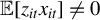 ${\mathbb {E}}[z_{it}x_{it}]\neq 0$
. The unit-wise IV estimators are given by
${\mathbb {E}}[z_{it}x_{it}]\neq 0$
. The unit-wise IV estimators are given by $\vartheta _{i, T} = (T^{-1}\sum _{t=1}^T z_{it}x_{it} )^{-1}T^{-1}\sum _{t=1}^T z_{it}y_{it}$
. In this case,
$\vartheta _{i, T} = (T^{-1}\sum _{t=1}^T z_{it}x_{it} )^{-1}T^{-1}\sum _{t=1}^T z_{it}y_{it}$
. In this case, $\varepsilon _{i, T} = (T^{-1}\sum _{t=1}^T z_{it}x_{it} )^{-1}T^{-1/2}\sum _{t=1}^T z_{it}u_{it}$
. Note that the distribution of
$\varepsilon _{i, T} = (T^{-1}\sum _{t=1}^T z_{it}x_{it} )^{-1}T^{-1/2}\sum _{t=1}^T z_{it}u_{it}$
. Note that the distribution of $\varepsilon _{i, T}$
may be strongly dissimilar to the normal distribution even for large T if
$\varepsilon _{i, T}$
may be strongly dissimilar to the normal distribution even for large T if $z_{it}$
is not a strong instrument (Nelson and Startz, Reference Nelson and Startz1990).
$z_{it}$
is not a strong instrument (Nelson and Startz, Reference Nelson and Startz1990).
Example 2 (Nonparametric Regression).
Let  for some fixed value $x_0$
. Let
$x_0$
. Let $\vartheta _{i, T} = (\sum _{t=1}^T K\left ({(x_{it}-x_0)}/{h} \right ) )^{-1}{\sum _{t=1}^T y_{it}K ({(x_{it}-x_0)}/{h} )}{}$
by the Nadaraya–Watson estimator of
$\vartheta _{i, T} = (\sum _{t=1}^T K\left ({(x_{it}-x_0)}/{h} \right ) )^{-1}{\sum _{t=1}^T y_{it}K ({(x_{it}-x_0)}/{h} )}{}$
by the Nadaraya–Watson estimator of $\theta _i$
, where K is a kernel function and h is a bandwidth parameter. Let
$\theta _i$
, where K is a kernel function and h is a bandwidth parameter. Let $u_{it} = y_{it} -\theta _i$
, and set
$u_{it} = y_{it} -\theta _i$
, and set $\varepsilon _{i, T} = (\sum _{t=1}^T K ({x_{it}-x_0}/{h} ) )^{-1}\sqrt {Th}\sum _{t=1}^T u_{it} K ({(x_{it}-x_0)}/{h} )$
. Let
$\varepsilon _{i, T} = (\sum _{t=1}^T K ({x_{it}-x_0}/{h} ) )^{-1}\sqrt {Th}\sum _{t=1}^T u_{it} K ({(x_{it}-x_0)}/{h} )$
. Let $h=T^{-s}, s\in (0, 1)$
. It holds that
$h=T^{-s}, s\in (0, 1)$
. It holds that $\varepsilon _{i, T}= O_p(1)$
and
$\varepsilon _{i, T}= O_p(1)$
and $\vartheta _{i, T} = \theta _i +T^{-(1-s)/2} \varepsilon _{i, T}$
under suitable conditions on h. If h is picked to optimize the convergence rate,
$\vartheta _{i, T} = \theta _i +T^{-(1-s)/2} \varepsilon _{i, T}$
under suitable conditions on h. If h is picked to optimize the convergence rate, $\varepsilon _{i, T}$
has a nonzero mean even in the limit.
$\varepsilon _{i, T}$
has a nonzero mean even in the limit.
Notation: Let $\vartheta _{1, N, T}\leq \dots \leq \vartheta _{N, N, T}$
be the order statistics of
$\vartheta _{1, N, T}\leq \dots \leq \vartheta _{N, N, T}$
be the order statistics of $ \left \lbrace {\vartheta _{1, T}, \dots , \vartheta _{N, T}} \right \rbrace $
, and similarly let
$ \left \lbrace {\vartheta _{1, T}, \dots , \vartheta _{N, T}} \right \rbrace $
, and similarly let $\theta _{1, N}\leq \dots \leq \theta _{N, N}$
be the order statistics of the latent noiseless
$\theta _{1, N}\leq \dots \leq \theta _{N, N}$
be the order statistics of the latent noiseless $ \left \lbrace {\theta _1, \dots , \theta _N} \right \rbrace $
.
$ \left \lbrace {\theta _1, \dots , \theta _N} \right \rbrace $
. $\Rightarrow $
denotes weak convergence, both of random variables and functions.
$\Rightarrow $
denotes weak convergence, both of random variables and functions.
2.3 Assumptions
Assumption 1. For each T, $ \left \lbrace {(\theta _i, \varepsilon _{i, T})} \right \rbrace _{i=1, \dots , N}$
are independent and identically distributed random vectors indexed by i.
$ \left \lbrace {(\theta _i, \varepsilon _{i, T})} \right \rbrace _{i=1, \dots , N}$
are independent and identically distributed random vectors indexed by i.
Observations $\vartheta _{i, T}$
are sampled in an IID fashion. Note that
$\vartheta _{i, T}$
are sampled in an IID fashion. Note that $\vartheta _{i, T}$
can be conditionally heteroskedastic:
$\vartheta _{i, T}$
can be conditionally heteroskedastic: ${\mathrm {Var}}(\vartheta _{i,T}|\theta _i)={\mathrm {Var}}(\varepsilon _{i, T}|\theta _i)$
can depend on
${\mathrm {Var}}(\vartheta _{i,T}|\theta _i)={\mathrm {Var}}(\varepsilon _{i, T}|\theta _i)$
can depend on $\theta _i$
, provided this variance exists.
$\theta _i$
, provided this variance exists.
Assumption 2. The distribution F of $\theta $
is in the weak domain of attraction of an EV distribution with EV index
$\theta $
is in the weak domain of attraction of an EV distribution with EV index $\gamma \in {\mathbb {R}}$
.
$\gamma \in {\mathbb {R}}$
.
Under Assumption 2, the classical EV theorem of Gnedenko (Reference Gnedenko1943) applies to the latent noiseless distribution F. This will serve as the basis for extending this EV convergence to the observed noisy data. Without Assumption 2, we would not be able to conduct inference using the asymptotic behavior of the sample maximum even if we had access to the true $\theta _i$
. Assumption 2 is a mild assumption, satisfied by almost all textbook continuous distributions and many discrete ones. Assumption 2 is equivalent to certain regular variation conditions on F (de Haan and Ferreira, Reference de Haan and Ferreira2006, Thm. 1.2.1).
$\theta _i$
. Assumption 2 is a mild assumption, satisfied by almost all textbook continuous distributions and many discrete ones. Assumption 2 is equivalent to certain regular variation conditions on F (de Haan and Ferreira, Reference de Haan and Ferreira2006, Thm. 1.2.1).
Two key features of our analysis are that we do not restrict the dependence structure between $\theta _i$
and
$\theta _i$
and $\varepsilon _{i, T}$
and that we impose no distributional assumptions on
$\varepsilon _{i, T}$
and that we impose no distributional assumptions on $\varepsilon _{i, T}$
. This approach is motivated by the following practical challenges. First,
$\varepsilon _{i, T}$
. This approach is motivated by the following practical challenges. First, $\theta _i$
and
$\theta _i$
and $\varepsilon _{i, T}$
will typically be related in a complex and unobservable manner outside of tightly controlled experimental settings. Such dependence may arise if the agent chooses some covariates with knowledge of
$\varepsilon _{i, T}$
will typically be related in a complex and unobservable manner outside of tightly controlled experimental settings. Such dependence may arise if the agent chooses some covariates with knowledge of $\theta _i$
, and these covariates are in turn used in the estimation of
$\theta _i$
, and these covariates are in turn used in the estimation of $\theta _i$
. Second, the distribution of
$\theta _i$
. Second, the distribution of $\varepsilon _{i, T}$
might not be well-approximated by a normal distribution, as in the IV case of Example 1 (though we show how to exploit normality of
$\varepsilon _{i, T}$
might not be well-approximated by a normal distribution, as in the IV case of Example 1 (though we show how to exploit normality of $\varepsilon _{i, T}$
).
$\varepsilon _{i, T}$
).
Instead, we only impose a weak assumption on the marginal distribution $G_T$
of
$G_T$
of $\varepsilon _{i, T}$
.
$\varepsilon _{i, T}$
.
Assumption 3 (Tightness of $ \left \lbrace {G_T} \right \rbrace _{T=1}^{\infty }$
).
$ \left \lbrace {G_T} \right \rbrace _{T=1}^{\infty }$
).

For any $\varepsilon>0,$
there exists some
$\varepsilon>0,$
there exists some $C_{\varepsilon }\geq 0$
such that for all
$C_{\varepsilon }\geq 0$
such that for all $T,$
it holds that
$T,$
it holds that $G_T(-C_{\varepsilon })\leq \varepsilon $
and
$G_T(-C_{\varepsilon })\leq \varepsilon $
and $1-G_T(C_{\varepsilon })\leq \varepsilon $
.
$1-G_T(C_{\varepsilon })\leq \varepsilon $
.
Intuitively, Assumption 3 requires that $\varepsilon _{i, T}$
be defined in such a way that, as
$\varepsilon _{i, T}$
be defined in such a way that, as $T\to \infty $
, the distributions
$T\to \infty $
, the distributions $G_T$
of
$G_T$
of $\varepsilon _{i, T}$
do not escape to infinity. Assumption 3 holds automatically if
$\varepsilon _{i, T}$
do not escape to infinity. Assumption 3 holds automatically if $T^p(\vartheta _{i, T}-\theta _i)$
has a non-degenerate asymptotic distribution. Together with definition (1), Assumption 3 implies that each
$T^p(\vartheta _{i, T}-\theta _i)$
has a non-degenerate asymptotic distribution. Together with definition (1), Assumption 3 implies that each $\vartheta _{i, T}$
is consistent for
$\vartheta _{i, T}$
is consistent for $\theta _i$
, but we allow
$\theta _i$
, but we allow $\vartheta _{i, T}$
to be biased in finite samples. In addition, Assumption 3 allows the mean of
$\vartheta _{i, T}$
to be biased in finite samples. In addition, Assumption 3 allows the mean of $\varepsilon _{i, T}$
to be nonzero in the limit, as may occur in nonparametric regression with MSE-minimizing choice of bandwidth (Example 2).
$\varepsilon _{i, T}$
to be nonzero in the limit, as may occur in nonparametric regression with MSE-minimizing choice of bandwidth (Example 2).
3 EXTREME VALUE THEORY FOR NOISY ESTIMATES
3.1 Extreme Value Theorem for Noisy Estimates
The key step toward inference on extreme quantiles is to establish distributional results for the sample maximum $\vartheta _{N, N, T}$
. The following result gives necessary and sufficient conditions under which
$\vartheta _{N, N, T}$
. The following result gives necessary and sufficient conditions under which $\vartheta _{N, N, T}$
and the latent maximum
$\vartheta _{N, N, T}$
and the latent maximum $\theta _{N, N}=\max \left \lbrace {\theta _1, \dots , \theta _N} \right \rbrace $
have the same limit distribution. It introduces the notion of tail equivalence (TE) and serves as a stepping stone toward our inference results.
$\theta _{N, N}=\max \left \lbrace {\theta _1, \dots , \theta _N} \right \rbrace $
have the same limit distribution. It introduces the notion of tail equivalence (TE) and serves as a stepping stone toward our inference results.
Theorem 3.1. Let Assumption 1 hold. Let constants $a_N, b_N$
and a random variable X be such that
$a_N, b_N$
and a random variable X be such that ${(\theta _{N, N} - b_N)}/{a_N}\Rightarrow X$
as
${(\theta _{N, N} - b_N)}/{a_N}\Rightarrow X$
as $N\to \infty $
. Let F be the cdf of
$N\to \infty $
. Let F be the cdf of $\theta _i$
and
$\theta _i$
and $G_{T}$
be the cdf of
$G_{T}$
be the cdf of $\varepsilon _{i, T}$
.
$\varepsilon _{i, T}$
.
-
(1) (Transferral of Convergence) Let the following TE conditions hold: for each
$\tau \in (0, \infty )$
as
$N, T\to \infty ,$
there exists some
$\epsilon \in (0, 1)$
(TE-Sup)
$$ \begin{align} & \hspace{0pt} \sup_{u\in \left[0, \epsilon\right]} \dfrac{1}{a_N}\left( F^{-1}\left(1- \dfrac{1}{N\tau}-u \right) -F^{-1}\left(1- \dfrac{1}{N\tau} \right) + \dfrac{1}{T^p} G_T^{-1}\left(u\right) \right) \to 0, & \end{align} $$
(TE-Inf)
$$ \begin{align} & \hspace{0pt} \inf_{u\in \left[0, \frac{1}{N\tau} \right]} \dfrac{1}{a_N}\left(F^{-1}\left(1- \dfrac{1}{N\tau} + u\right) - F^{-1}\left(1- \dfrac{1}{N\tau} \right) +\dfrac{1}{T^p} G_T^{-1}\left(1-u\right) \right) \to 0. & \end{align} $$
Then,
$ (\vartheta _{N, N, T}- b_N)/{a_N} \Rightarrow X$
as
$N, T\to \infty $
. -
(2) (Sharpness) Consider the following TE condition: for each
$\tau \in (0, \infty )$
as
$N, T\to \infty ,$
(TE-Sup')
$$ \begin{align} \sup_{u\in \left[0, 1-\frac{1}{N\tau}\right]} \dfrac{1}{a_N}\left( F^{-1}\left(1- \dfrac{1}{N\tau}-u \right) -F^{-1}\left(1- \dfrac{1}{N\tau} \right) + \dfrac{1}{T^p} G_T^{-1}\left(u\right) \right) \to 0. \end{align} $$
Then, (i) (TE-Sup) and (TE-Inf) together imply (TE-Sup') and (ii) (TE-Inf) and (TE-Sup') are sharp in the following sense: if at least one of the conditions fails, there exists a sequence of joint distributions of
$(\theta _i, \varepsilon _{i, T})$
with given marginal distributions
$F, G_T$
such that
$({\vartheta _{N, N, T}- b_N})/{a_N}$
weakly converges to a limit different from X or does not converge at all.


Theorem 3.1 establishes the precise conditions under which the maximum of the noisy sample, $\vartheta _{N, N, T}$
, inherits the asymptotic distribution of the latent maximum
$\vartheta _{N, N, T}$
, inherits the asymptotic distribution of the latent maximum $\theta _{N, N}$
. The result is general, holding regardless of the dependence structure between
$\theta _{N, N}$
. The result is general, holding regardless of the dependence structure between $\theta _i$
and
$\theta _i$
and $\varepsilon _{i, T}$
. If the TE conditions (TE-Sup') and (TE-Inf) fail, there exists at least one possible limiting distribution for
$\varepsilon _{i, T}$
. If the TE conditions (TE-Sup') and (TE-Inf) fail, there exists at least one possible limiting distribution for $\vartheta _{N, N, T}$
that differs from that of
$\vartheta _{N, N, T}$
that differs from that of $\theta _{N, N}$
, and convergence may occur only along a subsequence.
$\theta _{N, N}$
, and convergence may occur only along a subsequence.
At the core of this result are (TE-Sup) and (TE-Inf), which characterize the relationship between the right tails of the laws of $\vartheta _{i, T}$
and
$\vartheta _{i, T}$
and $\theta _i$
. These conditions ensure that, asymptotically, the noisy sample provides the same EV information as the unobserved noiseless sample. The expressions in (TE-Sup) and (TE-Inf) reflect a pointwise limit equivalence of tails: the term
$\theta _i$
. These conditions ensure that, asymptotically, the noisy sample provides the same EV information as the unobserved noiseless sample. The expressions in (TE-Sup) and (TE-Inf) reflect a pointwise limit equivalence of tails: the term $F^{-1} + T^{-p}G^{-1}$
captures the approximate quantiles of the noisy observations, while
$F^{-1} + T^{-p}G^{-1}$
captures the approximate quantiles of the noisy observations, while $(-F^{-1})$
are the quantiles of the target distribution. The supremum and infimum adjust for the unknown dependence between
$(-F^{-1})$
are the quantiles of the target distribution. The supremum and infimum adjust for the unknown dependence between $\theta _i$
and
$\theta _i$
and $\varepsilon _{i, T}$
.
$\varepsilon _{i, T}$
.
These TE conditions provide a general framework for EV analysis in the presence of noise. They accommodate a broad range of estimators for $\theta _i$
(see equation (1)), including linear, nonlinear, and nonparametric estimators. In addition, they sharpen and generalize the sufficient condition derived by Sasaki and Wang (Reference Sasaki and Wang2022) for the special case of univariate linear regression (see Remark 1 below).
$\theta _i$
(see equation (1)), including linear, nonlinear, and nonparametric estimators. In addition, they sharpen and generalize the sufficient condition derived by Sasaki and Wang (Reference Sasaki and Wang2022) for the special case of univariate linear regression (see Remark 1 below).
We highlight four aspects of conditions (TE-Sup) and (TE-Inf). First, the infimum in (TE-Inf) is always greater than or equal to the supremum values in (TE-Sup) and (TE-Sup'), as shown in the proof. Second, the conditions hold automatically in the absence of estimation noise. In this case, the function under the supremum in (TE-Sup) is non-positive for all admissible u, and equal to zero only at u = 0. Likewise, the function under the infimum in (TE-Inf) is nonnegative and zero only at u = 0. Third, when estimation noise is present, similar logic applies but the impact on the conditions is asymmetric: if G T (0) ∈ (0, 1), the function under the infimum is eventually always nonnegative, with (TE-Inf) requiring its minimum to converge to zero. Meanwhile, the function under the supremum in (TE-Sup) can be negative over some range of u but may change sign at larger values. Here, (TE-Sup) requires that the supremum converge to zero, whether from above or below. We stress that this is not a requirement of uniform convergence. Finally, for sharpness, the weaker condition (TE-Sup') is necessary. However, for practical purposes, (TE-Sup) is sufficient and more interpretable; it may be viewed as controlling the contribution of the left tail of G T .
When do (TE-Inf) and (TE-Sup) hold? Proposition 3.2 provides sufficient conditions, expressed as constraints on the growth rate of N relative to T, given assumptions on the tails of $G_T$
. Such conditions depend on
$G_T$
. Such conditions depend on $\gamma $
, the EV index of F, which is typically unknown. However, they remain valid when only a lower bound
$\gamma $
, the EV index of F, which is typically unknown. However, they remain valid when only a lower bound $\gamma ' \leq \gamma $
is available. Intuitively, when
$\gamma ' \leq \gamma $
is available. Intuitively, when $\gamma $
is large, F has a heavier tail, making the contribution of
$\gamma $
is large, F has a heavier tail, making the contribution of $G_T$
less pronounced and allowing for larger values of N.
$G_T$
less pronounced and allowing for larger values of N.
Proposition 3.2. Let Assumptions 1 and 3 hold. Let one of the following conditions hold:
-
(1) Let
$\sup _T{\mathbb {E}} \left \lvert {\varepsilon _{i, T}} \right \rvert ^{\beta }<\infty $
for some
$\beta>0$
, and let
${N^{1/\beta -\gamma '}(\log (T))^{1/\beta }}/{T^{p}}\to 0 $
for some
$\gamma '$
. -
(2) For all T, let
$\varepsilon _{i, T}\sim N(\mu _T, \sigma _T^2)$
, and let
${N^{-\gamma '} \sqrt {\log (N)}}/{T^{p}}\to 0 $
for some
$\gamma '$
.





In addition, let F satisfy Assumption 2 with EV index $\gamma>\gamma '$
. Then, (TE-Inf) and (TE-Sup) hold for F and
$\gamma>\gamma '$
. Then, (TE-Inf) and (TE-Sup) hold for F and $G_T$
for any sequence
$G_T$
for any sequence $ \left \lbrace {(a_N, b_N)} \right \rbrace _{N=1}^{\infty }$
such that
$ \left \lbrace {(a_N, b_N)} \right \rbrace _{N=1}^{\infty }$
such that $(\theta _{N, N}-b_N)/a_N$
converges to a non-degenerate random variable.
$(\theta _{N, N}-b_N)/a_N$
converges to a non-degenerate random variable.
Proposition 3.2 highlights two key factors that determine how restrictive these conditions are. First, heavier tails of F (larger $\gamma '$
) permit a larger N relative to T. Second, lighter tails of
$\gamma '$
) permit a larger N relative to T. Second, lighter tails of $G_T$
result in milder constraints on N. The conditions on
$G_T$
result in milder constraints on N. The conditions on $G_T$
are captured by (1) and (2). Condition (1) requires only that
$G_T$
are captured by (1) and (2). Condition (1) requires only that $G_T$
has uniformly bounded
$G_T$
has uniformly bounded $\beta $
th moments, while (2) assumes exact normality, which can be viewed as a limiting case of (1) as
$\beta $
th moments, while (2) assumes exact normality, which can be viewed as a limiting case of (1) as $\beta \to \infty $
. In practice,
$\beta \to \infty $
. In practice, $G_T$
is expected to lie between these two extremes, with its tails becoming lighter as
$G_T$
is expected to lie between these two extremes, with its tails becoming lighter as $T \to \infty $
.
$T \to \infty $
.
A useful comparison can be made to the conditions for inference on central quantiles established by Jochmans and Weidner (Reference Jochmans and Weidner2024). They show that $N/T^4 \to 0$
is sufficient for validity when
$N/T^4 \to 0$
is sufficient for validity when $p = 1/2$
, under broad conditions on F (see Theorem 4.6). A similar rate condition arises in our extreme setting when
$p = 1/2$
, under broad conditions on F (see Theorem 4.6). A similar rate condition arises in our extreme setting when $G_T$
has more than eight moments and
$G_T$
has more than eight moments and $\gamma \geq 0$
(as is necessarily the case if F has an infinite tail).Footnote
2
Proposition 3.2 also allows for nearly exponential growth of N relative to T when
$\gamma \geq 0$
(as is necessarily the case if F has an infinite tail).Footnote
2
Proposition 3.2 also allows for nearly exponential growth of N relative to T when $\varepsilon _{i,T}$
is normally distributed and
$\varepsilon _{i,T}$
is normally distributed and $\gamma \geq 0$
. This suggests that valid inference on extreme quantiles may still be feasible in cases where central quantile inference is not. Conversely, when
$\gamma \geq 0$
. This suggests that valid inference on extreme quantiles may still be feasible in cases where central quantile inference is not. Conversely, when $\gamma < 0$
, the sufficient conditions for TE may become more restrictive than those for central quantiles.
$\gamma < 0$
, the sufficient conditions for TE may become more restrictive than those for central quantiles.
Importantly, the TE conditions differ from the Jochmans and Weidner (Reference Jochmans and Weidner2024) conditions in their underlying mechanisms. The latter are primarily concerned with the rate of estimation noise bias, while the TE conditions control the relative contribution of the tail of F and the tails of $G_T$
. As a result, TE conditions benefit from lighter tails of
$G_T$
. As a result, TE conditions benefit from lighter tails of $G_T$
, and they hold trivially in the noiseless setting, as noted after Theorem 3.1.
$G_T$
, and they hold trivially in the noiseless setting, as noted after Theorem 3.1.
Remark 1 (Relation to Sasaki and Wang, Reference Sasaki and Wang2022).
Sasaki and Wang (Reference Sasaki and Wang2022) analyze the special case of univariate linear regression with heterogeneous coefficients (OLS in Example 1) and derive a condition similar to those in Proposition 3.2. Their condition 2.7 aligns closely with our result, modulo certain high-level uniformity assumptions which concern averages of residuals and covariates. In this linear case, Proposition 3.2 quantifies these uniformity conditions and shows that they impose an additional restriction that depends on $G_T$
, as reflected in the
$G_T$
, as reflected in the $N^{1/\beta }$
or
$N^{1/\beta }$
or $\log (N)$
terms.
$\log (N)$
terms.
Remark 2. An appropriate value of $\gamma '$
might often be apparent in a given application. For example, Gabaix (Reference Gabaix2009, Reference Gabaix2016) documents that many economic relations follow a power law and outlines some general theoretical mechanisms under which a power law arises. If such a mechanism is likely to hold in a given situation, it is reasonable to assume that the distribution of the data is well approximated by a power law. Since a power law distribution has to have
$\gamma '$
might often be apparent in a given application. For example, Gabaix (Reference Gabaix2009, Reference Gabaix2016) documents that many economic relations follow a power law and outlines some general theoretical mechanisms under which a power law arises. If such a mechanism is likely to hold in a given situation, it is reasonable to assume that the distribution of the data is well approximated by a power law. Since a power law distribution has to have $\gamma>0$
, it is sufficient to check the hypothesis of Proposition 3.2 with
$\gamma>0$
, it is sufficient to check the hypothesis of Proposition 3.2 with $\gamma '=0$
. Further, to allow the distribution of
$\gamma '=0$
. Further, to allow the distribution of $\theta $
to potentially have a light infinite tail, it is sufficient to check conditions for any
$\theta $
to potentially have a light infinite tail, it is sufficient to check conditions for any $\gamma '<0$
, potentially arbitrarily close to 0.
$\gamma '<0$
, potentially arbitrarily close to 0.
3.2 Intermediate Order Statistics
To conduct inference on extreme quantiles, we also need to develop an asymptotic theory for intermediate order statistics. Formally, $\theta _{N-k(N), N}$
is called an intermediate order statistic if
$\theta _{N-k(N), N}$
is called an intermediate order statistic if $k(N)\to \infty $
as
$k(N)\to \infty $
as $N\to \infty $
and
$N\to \infty $
and $k(N)=o(N)$
. Intuitively, such statistics asymptotically stay in the tail, but are not the top statistics. We generally suppress the dependence of k on N.
$k(N)=o(N)$
. Intuitively, such statistics asymptotically stay in the tail, but are not the top statistics. We generally suppress the dependence of k on N.
To derive asymptotic properties of intermediate order statistics, we impose an additional assumption on F that refines Assumption 2.
Assumption 4 (F satisfies a first-order von Mises condition).
F is twice differentiable with density f, f positive in some left neighborhood of $F^{-1}(1)$
(
$F^{-1}(1)$
( $F^{-1}(1)$
might be finite or infinite), and for some
$F^{-1}(1)$
might be finite or infinite), and for some $\gamma \in {\mathbb {R}},$
it holds that
$\gamma \in {\mathbb {R}},$
it holds that $ \lim _{t\uparrow F^{-1}(1)} \left ( [1-F]/{f}\right )'(t) =\gamma .$
Assumption 4 is a slight strengthening of Assumption 2. See Dekkers and Haan, Reference Dekkers and Haan1989 and de Haan and Ferreira, Reference de Haan and Ferreira2006 for a discussion of the condition and its plausibility.
We now state a theorem describing the asymptotic behavior of intermediate order statistics.
Theorem 3.3 (Intermediate Value Theorem).
Let Assumptions 1 and 4 hold and let $k=k(N)\to \infty , k=o(N)$
as
$k=k(N)\to \infty , k=o(N)$
as $N\to \infty $
. Define
$N\to \infty $
. Define $c_N$
as the derivative of the inverse of
$c_N$
as the derivative of the inverse of $1/(1-F)$
evaluated at
$1/(1-F)$
evaluated at $N/k$
and multiplied by
$N/k$
and multiplied by $N/k$
, that is,
$N/k$
, that is, $c_N= (N/k)\times \left [\left (\left ({1}/({1-F}) \right )^{-1}\right )'\left ( N/k \right )\right ]$
. Let
$c_N= (N/k)\times \left [\left (\left ({1}/({1-F}) \right )^{-1}\right )'\left ( N/k \right )\right ]$
. Let $U_1, \dots , U_N$
be iid Uniform[0, 1] random variables.
$U_1, \dots , U_N$
be iid Uniform[0, 1] random variables.
-
(1) (Transferral of convergence) Let the following TE conditions hold as
$N, T\to \infty $
for some
$\epsilon>0$
: (2)
$$ \begin{align} & \hspace{0pt} \sup_{u\in \left[0, \epsilon\right]} \dfrac{\sqrt{k}}{c_N} \left( F^{-1}(1-U_{k, N}-u) -F^{-1}\left(1- U_{k, N} \right) + \dfrac{1}{T^p} G_T^{-1}\left( u\right) \right) \xrightarrow{p} 0, \end{align} $$
(3)
$$ \begin{align} & \hspace{0pt} \inf_{u\in \left[0, U_{k, N}\right]} \dfrac{\sqrt{k}}{c_N } \left(F^{-1}\left(1- U_{k, N} + u \right) - F^{-1}\left(1- U_{k, N} \right) +\dfrac{1}{T^p} G_T^{-1}\left(1-u\right)\right) \xrightarrow{p} 0. \end{align} $$
Then, as
$N, T\to \infty ,$
(4)
$$ \begin{align} \dfrac{\sqrt{k}}{c_N} \left(\vartheta_{N-k, N, T} - F^{-1}\left(1- k/N\right) \right)\Rightarrow N(0, 1). \end{align} $$
-
(2) (Sharpness) Consider the following condition:
(5)
$$ \begin{align} \sup_{u\in \left[0, 1-U_{k, N }\right]} \dfrac{\sqrt{k}}{c_N} \left( F^{-1}(1-U_{k, N}-u) -F^{-1}\left(1- U_{k, N} \right) + \dfrac{1}{T^p} G_T^{-1}\left( u\right) \right) \xrightarrow{p} 0, \end{align} $$
Conditions (3) and (5) are sharp in the sense of Theorem 3.1.


Theorem 3.3 is the intermediate order counterpart of Theorem 3.1; conditions (2), (3), and (5) are analogs of (TE-Sup), (TE-Inf), and (TE-Sup'), respectively. The two sets of conditions differ in the region where TE is imposed. Theorem 3.1 concerns quantiles of the form $1- 1/(N\tau )$
,
$1- 1/(N\tau )$
, $\tau>0$
fixed, whereas Theorem 3.3 looks at quantiles of the order
$\tau>0$
fixed, whereas Theorem 3.3 looks at quantiles of the order $1-k/N$
. Since
$1-k/N$
. Since $k\to \infty $
, the two regions are asymptotically distinct. A second point of difference between the two pairs of conditions is that conditions of Theorem 3.3 take a randomized form, though Proposition 3.4 below provides deterministic sufficient conditions. As before, the conditions allow for general dependence structures and natures of
$k\to \infty $
, the two regions are asymptotically distinct. A second point of difference between the two pairs of conditions is that conditions of Theorem 3.3 take a randomized form, though Proposition 3.4 below provides deterministic sufficient conditions. As before, the conditions allow for general dependence structures and natures of $\varepsilon _{i, T}$
. To the best of our knowledge, there are no directly comparable results in the literature.Footnote
3
$\varepsilon _{i, T}$
. To the best of our knowledge, there are no directly comparable results in the literature.Footnote
3
As for (TE-Inf) and (TE-Sup), sufficient conditions for (2) and (3) take the form of rate restrictions on N and T that depend on the EV index $\gamma $
. A sufficient condition is possible if a lower bound for
$\gamma $
. A sufficient condition is possible if a lower bound for $\gamma $
is available. The following proposition is an analog of Proposition 3.2.
$\gamma $
is available. The following proposition is an analog of Proposition 3.2.
Proposition 3.4. Let Assumptions 1 and 3 hold. Let $\delta \in (0, 1)$
. Let one of the following conditions hold:
$\delta \in (0, 1)$
. Let one of the following conditions hold:
-
(1)
$\sup _T{\mathbb {E}} \left \lvert {\varepsilon _{i, T}} \right \rvert ^{\beta }<\infty $
and for some
$\nu>0, \gamma ',$
it holds that
${ N^{\delta /2(1+1/\beta ) + (1-\delta )(-\gamma '+1/\beta ) + \nu /\beta }}/{T^{p}} \to 0. $
-
(2) For all T let
$\varepsilon _{i, T}\sim N(\mu _T, \sigma _T^2)$
, and for some
$\gamma ',$
it holds that
$N^{\delta /2 + (1-\delta )(-\gamma ')} \sqrt {\log (N)}/{T^p}\to 0$
.


In addition, let F satisfy Assumption 4 with EV index $\gamma>\gamma '$
. Then, conditions (2) and (3) hold for F and
$\gamma>\gamma '$
. Then, conditions (2) and (3) hold for F and $G_T$
for
$G_T$
for $k=N^{\delta }$
.
$k=N^{\delta }$
.
Remark 3 (Comparison of Sufficient Conditions for the EVT and the IVT).
Depending on $\gamma $
, the rate conditions for the EVT may be more or less restrictive than the conditions for the IVT. For example, suppose that
$\gamma $
, the rate conditions for the EVT may be more or less restrictive than the conditions for the IVT. For example, suppose that $\varepsilon _{i\, T}$
is normally distributed. If
$\varepsilon _{i\, T}$
is normally distributed. If $\gamma \leq -1/2$
, then the EVT condition implies the IVT condition; the opposite holds if
$\gamma \leq -1/2$
, then the EVT condition implies the IVT condition; the opposite holds if $\gamma>-1/2$
, regardless of the value of
$\gamma>-1/2$
, regardless of the value of $\delta $
. In particular, if
$\delta $
. In particular, if $\gamma>0$
, for the EVT, there are no restrictions on the relative sizes of N and T, but there are restrictions for the IVT.
$\gamma>0$
, for the EVT, there are no restrictions on the relative sizes of N and T, but there are restrictions for the IVT.
Remark 4 (Dependence on
$\delta $
).

Conditions of Proposition 3.4 depend on $\delta $
, the parameter that determines the magnitude of
$\delta $
, the parameter that determines the magnitude of $k=N^{\delta }$
. If
$k=N^{\delta }$
. If $\delta $
is close to zero, conditions for the IVT are close to those for the EVT. Intuitively, in this case, conditions (2) and (3) require asymptotic TE in approximately the same section of the tail as conditions (TE-Sup) and (TE-Inf), and so the resulting sufficient conditions are similar. As
$\delta $
is close to zero, conditions for the IVT are close to those for the EVT. Intuitively, in this case, conditions (2) and (3) require asymptotic TE in approximately the same section of the tail as conditions (TE-Sup) and (TE-Inf), and so the resulting sufficient conditions are similar. As $\delta $
grows, the region controlled by conditions (2) and (3) becomes distinct from the right endpoint of the distribution (while still staying in the tails by the requirement that
$\delta $
grows, the region controlled by conditions (2) and (3) becomes distinct from the right endpoint of the distribution (while still staying in the tails by the requirement that $k=o(N)$
).
$k=o(N)$
).
4 INFERENCE USING NOISY ESTIMATES
We now turn to inference. In this section, we introduce CIs, estimators, and tests based on extreme and intermediate order asymptotic approximations. We also briefly discuss the central order approximations of Jochmans and Weidner (Reference Jochmans and Weidner2024).
The extreme, intermediate, and central order approximations differ in their appropriate use case. Let $\tau $
be the quantile of interest. Based on the simulation evidence of Section 5 and the Supplementary Material, we propose the following rule of thumb that is valid for all values of N:
$\tau $
be the quantile of interest. Based on the simulation evidence of Section 5 and the Supplementary Material, we propose the following rule of thumb that is valid for all values of N:
-
(1) If
$(1-\tau )N\leq 100$
and
$\tau \geq 0.9$
, we recommend extreme order approximations—the approach based on Theorem 4.3 below. In this case, fewer than 100 order statistics lie to the right of the sample
$\tau $
th quantile, and the central limit theorem for quantiles is unlikely to provide a good approximation. -
(2) If
$(1-\tau )N>100$
, we recommend using a central order approximation. Specifically, we recommend basing inference on Theorem 4.6 below.


In larger cross sections ( $N\gtrsim 10,000$
), the intermediate order approach of Theorem 4.5 is a viable and particularly simple-to-compute option for
$N\gtrsim 10,000$
), the intermediate order approach of Theorem 4.5 is a viable and particularly simple-to-compute option for $\tau \geq [0.9, 1)$
, provided the corresponding value of
$\tau \geq [0.9, 1)$
, provided the corresponding value of $k\equiv (1-\tau )N$
satisfies
$k\equiv (1-\tau )N$
satisfies $k\geq 100$
.
$k\geq 100$
.
4.1 Inference Using Extreme Order Approximations
Extreme order approximations use Theorem 3.1 as the basis for inference. The quantile of interest is modeled as drifting to 1 at a rate proportional to $N^{-1}$
. Formally, we select
$N^{-1}$
. Formally, we select $b_N = F^{-1}(1-l/N)$
in Theorem 3.1 for some fixed
$b_N = F^{-1}(1-l/N)$
in Theorem 3.1 for some fixed $l>0$
. Further, we make an explicit choice of scaling constants
$l>0$
. Further, we make an explicit choice of scaling constants $a_N$
. Then, the following version of Theorem 3.1 holds.
$a_N$
. Then, the following version of Theorem 3.1 holds.
Lemma 4.1. Let assumptions of Theorem 3.1 hold. Let $l>0$
be fixed. Let
$l>0$
be fixed. Let $E_1^*$
be a standard exponential random variable.
$E_1^*$
be a standard exponential random variable.
-
(1) If F satisfies Assumption 2 with EV index
$\gamma>0$
, then
$$ \begin{align*} \dfrac{1}{ F^{-1}\left( 1 - \frac{1}{N} \right)} \left[ \vartheta_{N, N, T}- F^{-1}\left( 1-\dfrac{l}{N} \right)\right] \Rightarrow (E_1^*)^{-\gamma} - l^{-\gamma}\text{ as } N, T\to\infty. \end{align*} $$
-
(2) If F satisfies Assumption 2 with EV index
$\gamma =0$
, there for some positive function
$\hat {f,}$
$$ \begin{align*} \dfrac{1}{\hat{f}\left(F^{-1}\left( 1 - \frac{1}{N} \right)\right)} \left( \vartheta_{N, N, T} - F^{-1}\left( 1 - \frac{l}{N} \right) \right) \Rightarrow -\log(E_1^*) {-} \log(l)\text{ as } N, T{\to}\infty. \end{align*} $$
-
(3) If F satisfies Assumption 2 with EV index
$\gamma <0$
, then
$F^{-1}(1)<\infty $
and
$$ \begin{align*} \!\!\!\dfrac{1}{F^{-1}(1) - F^{-1}\left(1- \frac{1}{N} \right) }\left(\vartheta_{N, N, T} - F^{-1}\!\left(\! 1- \frac{l}{N} \!\right) \!\right) {\Rightarrow} -(E_1^*)^{-\gamma} {+} l^{-\gamma}\text{ as } N, T{\to}\infty. \end{align*} $$


Lemma 4.1 cannot be used for inference directly, as the scaling constants involved are unknown. These constants involve the $(1-1/N)$
th quantile of F, and so are not covered by sample information.
$(1-1/N)$
th quantile of F, and so are not covered by sample information.
To address this challenge, we first establish an intermediate result. The following lemma extends Theorem 3.1 to cover a vector of q top order statistics for q fixed.
Lemma 4.2 (Joint EVT).
Let assumptions of Theorem 3.1 hold. Let q be a fixed natural number and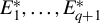 $E_1^*, \dots , E_{q+1}^*$
be iid standard exponential random variables.
$E_1^*, \dots , E_{q+1}^*$
be iid standard exponential random variables.
-
(1) If F satisfies Assumption 2 with
$\gamma>0$
, then as
$N, T\to \infty $
$$ \begin{align*} &\begin{pmatrix} \dfrac{\vartheta_{N, N, T}}{ F^{-1}(1-1/N)}, \dfrac{\vartheta_{N-1, N, T} }{ F^{-1}(1-1/N)}, \dots, \dfrac{\vartheta_{N-q, N, T} }{ F^{-1}(1-1/N)} \end{pmatrix} \\ &\quad \Rightarrow \begin{pmatrix} {(E_1^*)^{-\gamma} }, {(E_1^*+E_2^*)^{-\gamma} }, \dots, {(E_1^*+E_2^*+ \dots + E^*_{q+1})^{-\gamma} } \end{pmatrix}. \end{align*} $$
-
(2) If F satisfies Assumption 2 with
$\gamma =0$
, then as
$N, T\to \infty $
for
$\hat {f}$
as in Lemma 4.1
$$ \begin{align*} \begin{pmatrix} \dfrac{ \vartheta_{N, N, T} - F^{-1}\left( 1 - \frac{1}{N} \right)}{\hat{f}\left(F^{-1}\left( 1 - \frac{1}{N} \right)\right)} , \dfrac{ \vartheta_{N-1, N, T} - F^{-1}\left( 1 - \frac{1}{N} \right)}{\hat{f}\left(F^{-1}\left( 1 - \frac{1}{N} \right)\right)}, \dots, \dfrac{ \vartheta_{N-q, N, T} - F^{-1}\left( 1 - \frac{1}{N} \right)}{\hat{f}\left(F^{-1}\left( 1 - \frac{1}{N} \right)\right)} \end{pmatrix} \\ \Rightarrow \begin{pmatrix} {-\log(E_1^*) }, {-\log(E_1^*+E_2^*)}, \dots, {-\log(E_1^*+E_2^*+ \dots + E^*_{q+1}) } \end{pmatrix}. \end{align*} $$
-
(3) If F satisfies Assumption 2 with EV index
$\gamma <0$
, then as
$N, T\to \infty $
$$ \begin{align*} \begin{pmatrix} \dfrac{\vartheta_{N, N, T}-F^{-1}(1)}{F^{-1}(1) - F^{-1}(1-1/N)}, \dfrac{\vartheta_{N-1, N, T} -F^{-1}(1)}{F^{-1}(1) - F^{-1}(1-1/N)}, \dots, \dfrac{\vartheta_{N-q, N, T } -F^{-1}(1)}{F^{-1}(1) - F^{-1}(1-1/N)} \end{pmatrix} \\ \Rightarrow \begin{pmatrix} {-(E_1^*)^{-\gamma} }, -{(E_1^*+E_2^*)^{-\gamma} }, \dots, -{(E_1^*+E_2^*+ \dots + E^*_{q+1})^{-\gamma} } \end{pmatrix}. \end{align*} $$


Lemma 4.2 allows us to solve the issue of unknown scaling rates by using a self-normalization trick similar to the one employed by Chernozhukov and Fernández-Val (Reference Chernozhukov and Fernández-Val2011) for quantile regression. By taking the ratio of two elements in the joint EVT 4.2, we eliminate scaling factors completely, while the form of the limit is explicitly known up to the EV index $\gamma $
.
$\gamma $
.
Combining Lemmas 4.1 and 4.2, we obtain the following version of the EVT that can be used to conduct inference on extreme quantiles under TE conditions.
Theorem 4.3 (Feasible EVT).
Let assumptions of Theorem 3.1 hold, in particular, let F have EV index $\gamma \in {\mathbb {R}}$
. Let
$\gamma \in {\mathbb {R}}$
. Let $q\geq 1, r\geq 0$
be fixed integers and
$q\geq 1, r\geq 0$
be fixed integers and $l> 0$
be a fixed real number; let
$l> 0$
be a fixed real number; let $E_1^*, E_2^*, \dots $
be iid standard exponential RVs. Then, as
$E_1^*, E_2^*, \dots $
be iid standard exponential RVs. Then, as $N, T\to \infty ,$
 $$ \begin{align} \dfrac{\vartheta_{N-r, N, T}- F^{-1}\left( 1- \frac{l}{N} \right) }{\vartheta_{N-q, N, T}-\vartheta_{N, N, T}} & \Rightarrow \dfrac{ (E_1^*+ \dots + E_{r+1}^*)^{-\gamma}- l^{-\gamma}}{(E_1^*+ \dots + E_{q+1}^*)^{-\gamma}-(E_1^*)^{-\gamma} } , \end{align} $$
where for $\gamma =0,$
the right-hand side means
$\gamma =0,$
the right-hand side means $[\log (E_1^* )-\log (l)]/[\log (E_1^*+ \dots + E_{q+1}^*)- \log (E_1^*) ]$
. In addition, if F satisfies Assumption 2 with
$[\log (E_1^* )-\log (l)]/[\log (E_1^*+ \dots + E_{q+1}^*)- \log (E_1^*) ]$
. In addition, if F satisfies Assumption 2 with $\gamma <0$
, then
$\gamma <0$
, then $F^{-1}(1)<\infty $
and we may set
$F^{-1}(1)<\infty $
and we may set $l=0$
in equation (6).
$l=0$
in equation (6).
Theorem 4.3 allows us to conduct inference on extreme quantiles with no knowledge of the value of $\gamma $
. The left-hand side of equation (6) does not depend on
$\gamma $
. The left-hand side of equation (6) does not depend on $\gamma $
; this statistic is the basis of our inference procedures. While the right-hand side limit distribution of equation (6) is non-pivotal and does depend on
$\gamma $
; this statistic is the basis of our inference procedures. While the right-hand side limit distribution of equation (6) is non-pivotal and does depend on $\gamma $
, we show below how the critical values can be consistently estimated either by subsampling without estimating
$\gamma $
, we show below how the critical values can be consistently estimated either by subsampling without estimating $\gamma $
(Theorem 4.4) or by plugging in a consistent estimator for
$\gamma $
(Theorem 4.4) or by plugging in a consistent estimator for $\gamma $
(Remarks 6 and 7).
$\gamma $
(Remarks 6 and 7).
We show how to construct CIs, estimators, and hypothesis tests for extreme quantiles based on Theorem 4.3 with a series of examples.
Example 3 (Location-Scale Equivariant CI for 95th Percentile).
Let $l=10$
and
$l=10$
and $N=200$
, in which case
$N=200$
, in which case $F^{-1}(1-l/N)=F^{-1}(0.95)$
. There are only ten observations to the right of the sample quantile, and it is appropriate to use the extreme order approximation described by Theorem 4.3. Let
$F^{-1}(1-l/N)=F^{-1}(0.95)$
. There are only ten observations to the right of the sample quantile, and it is appropriate to use the extreme order approximation described by Theorem 4.3. Let $q\geq 1$
,
$q\geq 1$
, $r \geq 0$
be fixed integers, see Remark 8 below on choice of r and q. Let
$r \geq 0$
be fixed integers, see Remark 8 below on choice of r and q. Let $\hat {c}_{\alpha }$
be a consistent estimator of the
$\hat {c}_{\alpha }$
be a consistent estimator of the $\alpha $
th quantile of
$\alpha $
th quantile of $ [ (E_1^* + \dots + E_{r+1}^*)^{-\gamma } - 10^{-\gamma } ]/ [(E_1^*+ \dots + E_{q+1}^*)^{-\gamma }- (E_1^*)^{-\gamma } ]$
. Then, let the CI for
$ [ (E_1^* + \dots + E_{r+1}^*)^{-\gamma } - 10^{-\gamma } ]/ [(E_1^*+ \dots + E_{q+1}^*)^{-\gamma }- (E_1^*)^{-\gamma } ]$
. Then, let the CI for $F^{-1}(0.95)$
based on sample size
$F^{-1}(0.95)$
based on sample size $N=200$
be given by
$N=200$
be given by
 $$ \begin{align*} CI_{\alpha}=\left[ \vartheta_{N-r, N, T} - \hat{c}_{\alpha/2} \left(\vartheta_{N-q, N, T} - \vartheta_{N, N, T} \right), \vartheta_{N-r, N, T} - \hat{c}_{1-\alpha/2} \left(\vartheta_{N-q, N, T} - \vartheta_{N, N, T} \right) \right]. \end{align*} $$ $CI_{\alpha }$
is location-scale equivariant, as the statistic of equation (6) is location-scale invariant.
$CI_{\alpha }$
is location-scale equivariant, as the statistic of equation (6) is location-scale invariant.
Care must be exercised in interpreting the asymptotic properties of $CI_{\alpha }$
: it is a
$CI_{\alpha }$
: it is a $(1-\alpha )\times 100\%$
asymptotic CIs for
$(1-\alpha )\times 100\%$
asymptotic CIs for $F^{-1}\left (1-l/N \right )$
. The target quantity shifts with N, and the value of l determines which quantile is targeted for a given sample size.
$F^{-1}\left (1-l/N \right )$
. The target quantity shifts with N, and the value of l determines which quantile is targeted for a given sample size.
Example 4 (Median-Unbiased Estimator for 95th Percentile).
Let $q, r$
, and
$q, r$
, and $\hat {c}_{\alpha }$
be as in example (3). By Theorem 4.3,
$\hat {c}_{\alpha }$
be as in example (3). By Theorem 4.3, $ P( ({\vartheta _{N-r, N, T}- F^{-1}(1-l/N) })/(\vartheta _{N-q, N, T}-\vartheta _{N, N, T}) \leq \hat {c}_{1/2} ) \to 1/2$
. Rearranging, we obtain that the estimator
$ P( ({\vartheta _{N-r, N, T}- F^{-1}(1-l/N) })/(\vartheta _{N-q, N, T}-\vartheta _{N, N, T}) \leq \hat {c}_{1/2} ) \to 1/2$
. Rearranging, we obtain that the estimator
 $$ \begin{align} \mathcal{M}_{N, T} = \vartheta_{N-r, N, T} - \hat{c}_{1/2} ( \vartheta_{N-q, N, T} - \vartheta_{N, N, T} ) \end{align} $$
is asymptotically median-unbiased for $F^{-1}(1-l/N)$
(see Chernozhukov and Fernández-Val, Reference Chernozhukov and Fernández-Val2011 for a similar construction in a quantile regression setting). Note that
$F^{-1}(1-l/N)$
(see Chernozhukov and Fernández-Val, Reference Chernozhukov and Fernández-Val2011 for a similar construction in a quantile regression setting). Note that $\mathcal {M}_{N, T}$
is always contained in
$\mathcal {M}_{N, T}$
is always contained in $CI_{\alpha }$
(unlike
$CI_{\alpha }$
(unlike $\vartheta _{N-r, N, T}$
which lies in
$\vartheta _{N-r, N, T}$
which lies in $CI_{\alpha }$
if
$CI_{\alpha }$
if $\hat {c}_{\alpha /2}$
and
$\hat {c}_{\alpha /2}$
and $\hat {c}_{1-\alpha /2}$
have different signs).
$\hat {c}_{1-\alpha /2}$
have different signs).
Example 5 (Hypothesis Tests About Support).
We can also use Theorem 4.3 to test hypotheses about the support of F. Let $\gamma <0$
and suppose we wish to test
$\gamma <0$
and suppose we wish to test $H_0: F^{-1}(1)\leq C$
vs.
$H_0: F^{-1}(1)\leq C$
vs. $H_1: F^{-1}(1)>C$
. Define the test statistic
$H_1: F^{-1}(1)>C$
. Define the test statistic $ W_C= {(\vartheta _{N, N, T}- C)}/{(\vartheta _{N-q, N, T} -\vartheta _{N, N, T})}.$
The test rejects
$ W_C= {(\vartheta _{N, N, T}- C)}/{(\vartheta _{N-q, N, T} -\vartheta _{N, N, T})}.$
The test rejects $H_0$
if
$H_0$
if $W_C<\hat {c}_{\alpha }$
, where
$W_C<\hat {c}_{\alpha }$
, where $\hat {c}_{\alpha }$
is a consistent estimator of the
$\hat {c}_{\alpha }$
is a consistent estimator of the $\alpha $
th quantile of
$\alpha $
th quantile of ${ (E_1^*)^{-\gamma } }/[{(E_1^*+ \dots + E_{q+1}^*)^{-\gamma }-(E_1^*)^{-\gamma } }]$
. The test is asymptotically size
${ (E_1^*)^{-\gamma } }/[{(E_1^*+ \dots + E_{q+1}^*)^{-\gamma }-(E_1^*)^{-\gamma } }]$
. The test is asymptotically size $\alpha $
and consistent against point alternatives, since
$\alpha $
and consistent against point alternatives, since $P(W_C<\hat {c}_{\alpha }|F^{-1}(1)=C)\to \alpha $
, and for any
$P(W_C<\hat {c}_{\alpha }|F^{-1}(1)=C)\to \alpha $
, and for any $\delta>0$
,
$\delta>0$
, $P(W_C<\hat {c}_{\alpha }|F^{-1}(1)=C-\delta ) \to 0$
,
$P(W_C<\hat {c}_{\alpha }|F^{-1}(1)=C-\delta ) \to 0$
, $P(W_C<\hat {c}_{\alpha }|F^{-1}(1)=C+\delta ) \to 1$
.
$P(W_C<\hat {c}_{\alpha }|F^{-1}(1)=C+\delta ) \to 1$
.
We now describe a subsampling estimator for the limit distribution of Theorem 4.3 (Politis and Romano, Reference Politis and Romano1994; Politis, Romano, and Wolf, Reference Politis, Romano and Wolf1999). Let $q>1, r\geq 0$
, and
$q>1, r\geq 0$
, and $l\geq 0$
. Define
$l\geq 0$
. Define $J(x)$
to be the limit distribution in equation (6). Split the set of units
$J(x)$
to be the limit distribution in equation (6). Split the set of units $ \left \lbrace {1, \dots , N} \right \rbrace $
into all subsamples of size b and index the subsamples by s,
$ \left \lbrace {1, \dots , N} \right \rbrace $
into all subsamples of size b and index the subsamples by s, $s=1, \dots , \binom {N}{b}$
(see Remark 5 below on the choice of b). Let
$s=1, \dots , \binom {N}{b}$
(see Remark 5 below on the choice of b). Let $\vartheta ^{(s)}_{b-k, b, T}$
be the
$\vartheta ^{(s)}_{b-k, b, T}$
be the $(b-k)$
th order statistic in subsample s. Define the subsampling estimator
$(b-k)$
th order statistic in subsample s. Define the subsampling estimator $L_{b, N, T}$
for J as
$L_{b, N, T}$
for J as
 $$ \begin{align*} L_{b, N, T}(x) & = \dfrac{1}{\binom{N}{b}}\sum_{s=1}^{\binom{N}{b}} {\mathbb{I}} \left\lbrace { W_{s, b, N, T}\leq x } \right\rbrace ,\!\! \quad W_{s, b, N, T} = \dfrac{ \vartheta_{b-r, b, T}^{(s)} - \vartheta_{N-Nl/b, N, T} }{\vartheta_{b-q, b, T}^{(s)} - \vartheta_{b, b, T}^{(s)} }, \quad\!\! \dfrac{Nl}{b}\leq N. \end{align*} $$
Observe that the subsample statistic $W_{s, b, N, T}$
is centered at
$W_{s, b, N, T}$
is centered at $\vartheta _{N-Nl/b, N, T}$
. Intuitively, this corresponds to the
$\vartheta _{N-Nl/b, N, T}$
. Intuitively, this corresponds to the $(1-l/b)$
th quantile, correctly centering the subsampled statistics. If we are interested in
$(1-l/b)$
th quantile, correctly centering the subsampled statistics. If we are interested in $F^{-1}(1)$
, then
$F^{-1}(1)$
, then $l=0$
, and the statistic is centered at
$l=0$
, and the statistic is centered at $\vartheta _{N, N, T}$
.
$\vartheta _{N, N, T}$
.
Define the estimated critical value $\hat {c}_{\alpha }$
as the
$\hat {c}_{\alpha }$
as the $\alpha $
th quantile of
$\alpha $
th quantile of $L_{b, N, T}$
. The following result shows that
$L_{b, N, T}$
. The following result shows that $\hat {c}_{\alpha }$
is consistent for the true critical values of interest for all
$\hat {c}_{\alpha }$
is consistent for the true critical values of interest for all $\alpha \in (0, 1)$
.
$\alpha \in (0, 1)$
.
Theorem 4.4. Let $b=N^m, m \in (0, 1)$
. If
$b=N^m, m \in (0, 1)$
. If $l>0$
, let the conditions of Propositions 3.2 and 3.4 hold with
$l>0$
, let the conditions of Propositions 3.2 and 3.4 hold with $\delta =1-m$
. If
$\delta =1-m$
. If $\gamma <0$
and
$\gamma <0$
and $l=0$
, then let conditions of Proposition 3.2 hold. Then, the subsampling estimator
$l=0$
, then let conditions of Proposition 3.2 hold. Then, the subsampling estimator $L_{b, N, T}(x)\xrightarrow {p} J(x)$
at all x and
$L_{b, N, T}(x)\xrightarrow {p} J(x)$
at all x and $\hat {c}_{\alpha }\xrightarrow {p} c_{\alpha }= J^{-1}(\alpha )$
for all
$\hat {c}_{\alpha }\xrightarrow {p} c_{\alpha }= J^{-1}(\alpha )$
for all $\alpha \in (0, 1)$
.
$\alpha \in (0, 1)$
.
Theorem 4.4 shows that subsampling may be applied in the case of noisy observations. The key step in establishing the validity of subsampling is to control the estimation noise in the subsamples and to leverage TE. Theorem 4.4 parallels a result derived by Chernozhukov and Fernández-Val (Reference Chernozhukov and Fernández-Val2011) for inference in extreme quantile regression.
Remark 5 (Choice of b).
We suggest two possible approaches for choosing b: a minimal interval volatility criterion (Romano and Wolf, Reference Romano and Wolf2001, Algorithm 5.1) and a criterion based on the stability of the subsampled distribution (Bickel and Sakov, Reference Bickel and Sakov2008, p. 971). In both cases, subsampling is applied for a range of candidate values of b. The value of b is selected by minimizing an approach-specific variability criterion. The former approach minimizes the variance of the endpoints of the CIs. The latter one minimizes the distance between the subsampling distributions for pairs of consecutive candidate values of b. Provided the conditions of Theorem 4.4 hold for each candidate value of b, either approach will select a valid b. In the simulations of Section 5, choosing b with the minimal volatility method leads to favorable performance of CIs.
Remark 6 (Estimation of the EV index).
Inference based on Theorem 4.3 does not require an estimate of $\gamma $
. However,
$\gamma $
. However, $\gamma $
may be consistently estimated. Let
$\gamma $
may be consistently estimated. Let $k=k(N)$
satisfy
$k=k(N)$
satisfy $k\to \infty , k=o(N)$
. Let
$k\to \infty , k=o(N)$
. Let $A_{N, T} =k^{-1}\sum _{i=0}^{k-1} \vartheta _{N-i, N, T}- \vartheta _{N-k, N, T}$
and
$A_{N, T} =k^{-1}\sum _{i=0}^{k-1} \vartheta _{N-i, N, T}- \vartheta _{N-k, N, T}$
and $B_{N, T} = k^{-2}\sum _{i=0}^{k-1} i \left ( \vartheta _{N-i, N, T}- \vartheta _{N-k, N, T}\right )$
. The Hill (Reference Hill1975) estimator
$B_{N, T} = k^{-2}\sum _{i=0}^{k-1} i \left ( \vartheta _{N-i, N, T}- \vartheta _{N-k, N, T}\right )$
. The Hill (Reference Hill1975) estimator $\hat {\gamma }_H$
and probability weighted moment (PWM) estimator
$\hat {\gamma }_H$
and probability weighted moment (PWM) estimator $\hat {\gamma }_{PWM}$
of Hosking and Wallis (Reference Hosking and Wallis1987) are defined as
$\hat {\gamma }_{PWM}$
of Hosking and Wallis (Reference Hosking and Wallis1987) are defined as
 $$ \begin{align*} \hat{\gamma}_H & = \dfrac{1}{k} \sum_{i=0}^{k-1} \log (\vartheta_{N-i, N, T} ) - \log(\vartheta_{N-k, N, T}), \quad \hat{\gamma}_{PWM} = \dfrac{A_{N, T}- 4 B_{N, T}}{A_{N, T}- 2B_{N, T}}. \end{align*} $$
If conditions of Theorems 3.1 and 3.3 hold, then $\hat {\gamma }_H\xrightarrow {p} \gamma $
if
$\hat {\gamma }_H\xrightarrow {p} \gamma $
if $\gamma> 0$
;
$\gamma> 0$
; $\hat {\gamma }_{PWM}\xrightarrow {p}\gamma $
if
$\hat {\gamma }_{PWM}\xrightarrow {p}\gamma $
if $\gamma <1$
(approximately if F has a finite first moment). The proof of consistency is given in the Proofs of Results in the Appendix. In practice, the value of k may be chosen in a data-driven way, and Caeiro and Gomes (Reference Caeiro and Gomes2016) discuss a number of approaches. In our simulations, we use the modified semiparametric bootstrap of Caers, Beirlant, and Maes (Reference Caers, Beirlant and Maes1999) (Caeiro and Gomes, Reference Caeiro and Gomes2016, Algorithm 4.3).
$\gamma <1$
(approximately if F has a finite first moment). The proof of consistency is given in the Proofs of Results in the Appendix. In practice, the value of k may be chosen in a data-driven way, and Caeiro and Gomes (Reference Caeiro and Gomes2016) discuss a number of approaches. In our simulations, we use the modified semiparametric bootstrap of Caers, Beirlant, and Maes (Reference Caers, Beirlant and Maes1999) (Caeiro and Gomes, Reference Caeiro and Gomes2016, Algorithm 4.3).
Remark 7 (Simulated Critical Values).
Estimating $\gamma $
provides a second way of estimating the critical values necessary for application of Theorem 4.3. Simulation-based critical values can be obtained by drawing samples from the limit distribution of equation (6) after plugging in
$\gamma $
provides a second way of estimating the critical values necessary for application of Theorem 4.3. Simulation-based critical values can be obtained by drawing samples from the limit distribution of equation (6) after plugging in $\hat {\gamma }_H$
or
$\hat {\gamma }_H$
or $\hat {\gamma }_{PWM}$
in place of
$\hat {\gamma }_{PWM}$
in place of $\gamma $
.
$\gamma $
.
Remark 8 (Choice of r and q).
Applying the methods of Examples 3–5 requires choosing the tuning parameters r and q. We suggest the following choices. For $N\leq 5,000$
, we suggest taking
$N\leq 5,000$
, we suggest taking $q=2$
with subsampled critical values, and
$q=2$
with subsampled critical values, and $q\in [2, 4]$
with simulated critical values. For larger cross sections, larger values of q may be taken, up to
$q\in [2, 4]$
with simulated critical values. For larger cross sections, larger values of q may be taken, up to $q=30$
. In both cases, the numerator parameter r should be picked to match
$q=30$
. In both cases, the numerator parameter r should be picked to match $\vartheta _{N-r, N, T}$
to the sample
$\vartheta _{N-r, N, T}$
to the sample $\tau $
th quantile, that is,
$\tau $
th quantile, that is, $r= \left \lfloor {(1-\tau )N} \right \rfloor $
. While this choice of r is somewhat improper in the context of Theorem 4.3, we note that
$r= \left \lfloor {(1-\tau )N} \right \rfloor $
. While this choice of r is somewhat improper in the context of Theorem 4.3, we note that $r\leq 100$
regardless of N under the rule of thumb outlined at the beginning of Section 4. The simulations of Section 5 and the Supplementary Material show that these choices yield favorable coverage and length properties.
$r\leq 100$
regardless of N under the rule of thumb outlined at the beginning of Section 4. The simulations of Section 5 and the Supplementary Material show that these choices yield favorable coverage and length properties.
Remark 9. An alternative approach for constructing CIs for extreme quantiles using an extreme order approximation is proposed by Müller and Wang (Reference Müller and Wang2017). They use Lemma 4.2 as the foundation of inference by treating the vector of top q order statistics as a single draw from the corresponding limit distribution. Based on such a joint EVT, Müller and Wang (Reference Müller and Wang2017) propose two methods: inverting the likelihood ratio and minimizing the average expected length where the average is taken over a pre-specified range of values for $\gamma $
. Both methods lead to valid CIs for extreme quantiles in our setting, as long as Lemma 4.2 holds; though we suggest using CIs based on Theorem 4.3 that require no optimization and no bounds on the parameter
$\gamma $
. Both methods lead to valid CIs for extreme quantiles in our setting, as long as Lemma 4.2 holds; though we suggest using CIs based on Theorem 4.3 that require no optimization and no bounds on the parameter $\gamma $
.
$\gamma $
.
4.2 Inference Using Intermediate Order Approximations
The intermediate order approximation of Theorem 3.3 provides an alternative approach to inference that is based on convergence of intermediate order statistics (equation (4)). In this case, the quantile of interest is modeled as drifting to 1 at a rate $k/N,$
where
$k/N,$
where $k\to \infty , k=o(N)$
as
$k\to \infty , k=o(N)$
as $N\to \infty $
; this rate is slower than the rate
$N\to \infty $
; this rate is slower than the rate $N^{-1}$
of extreme order approximations. The resulting statistic is asymptotically standard normal.
$N^{-1}$
of extreme order approximations. The resulting statistic is asymptotically standard normal.
To eliminate the unknown scaling rate $c_N$
, we again use an additional order statistic.Footnote
4
Unlike Theorem 4.3, the statistics in the denominator of the self-normalized statistic are asymptotically perfectly dependent and only differ by a nonzero deterministic factor. The following theorem first establishes that such a technique works in the noiseless case, which may be of independent interest; the result is then transferred to noisy observables.
$c_N$
, we again use an additional order statistic.Footnote
4
Unlike Theorem 4.3, the statistics in the denominator of the self-normalized statistic are asymptotically perfectly dependent and only differ by a nonzero deterministic factor. The following theorem first establishes that such a technique works in the noiseless case, which may be of independent interest; the result is then transferred to noisy observables.
Theorem 4.5. Let Assumptions 1 and 4 hold. Let $k=o(N), k\to \infty $
. Let
$k=o(N), k\to \infty $
. Let $f=F'$
be non-increasing or non-decreasing in some left neighborhood of
$f=F'$
be non-increasing or non-decreasing in some left neighborhood of $F^{-1}(1) (F^{-1}(1)\leq \infty )$
.
$F^{-1}(1) (F^{-1}(1)\leq \infty )$
.
-
(1) Then,
$$ \begin{align*} \dfrac{\theta_{N-k, N}- F^{-1}\left(1- \frac{k}{N} \right)}{\theta_{N-k, N}-\theta_{N-k- \left\lfloor {\sqrt{k}} \right\rfloor , N}} \Rightarrow N(0, 1), \quad N\to\infty. \end{align*} $$
-
(2) In addition, let conditions of Theorem 3.3 hold when evaluated at k and
$k+\sqrt {k}$
. Then, (8)
$$ \begin{align} \dfrac{\vartheta_{N-k, N, T}- F^{-1}(1-k/N)}{\vartheta_{N-k, N, T}-\vartheta_{N-k- \left\lfloor {\sqrt{k}} \right\rfloor , N, T}} \Rightarrow N(0, 1), \quad N, T\to\infty. \end{align} $$


The statistics of Theorem 4.5 are particularly simple to use. First, the limiting distribution does not involve any unknown parameters. Second, these statistics do not involve any tuning parameters. The choice of k determines the centering quantile of interest. When k is chosen, the denominator is uniquely determined by k:
Example 6. Let $N=200$
and let
$N=200$
and let $k=k(N)$
be such that
$k=k(N)$
be such that $k(200)=16$
and
$k(200)=16$
and $k\to \infty , k=o(N)$
as
$k\to \infty , k=o(N)$
as $N\to \infty $
. Then, by Theorem 4.5, a CI for
$N\to \infty $
. Then, by Theorem 4.5, a CI for $F^{-1}(0.92)$
based on sample of size
$F^{-1}(0.92)$
based on sample of size $N=200$
:
$N=200$
:

where $z_{\alpha }$
the
$z_{\alpha }$
the $\alpha $
th quantile of the standard normal distribution.
$\alpha $
th quantile of the standard normal distribution.
Remark 10 (Limitations of Theorem 4.5).
The approximation of Theorem 4.5 should not be used if k or N are small. If $ \left \lfloor {\sqrt {k}} \right \rfloor $
is small but positive,
$ \left \lfloor {\sqrt {k}} \right \rfloor $
is small but positive, $\vartheta _{N-k, N}$
and
$\vartheta _{N-k, N}$
and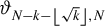 $\vartheta _{N-k- \left \lfloor {\sqrt {k}} \right \rfloor , N}$
will be close, and the distribution of the statistic may be far from normality. If
$\vartheta _{N-k- \left \lfloor {\sqrt {k}} \right \rfloor , N}$
will be close, and the distribution of the statistic may be far from normality. If $ \left \lfloor {\sqrt {k}} \right \rfloor =0$
, the statistic cannot be used. Since k must satisfy
$ \left \lfloor {\sqrt {k}} \right \rfloor =0$
, the statistic cannot be used. Since k must satisfy $k=o(N)$
, N must also be suitably large. A value of
$k=o(N)$
, N must also be suitably large. A value of $k\approx 100$
is generally the minimum threshold for Theorem 4.5 to provide a useful approximation, coupled with the requirement that
$k\approx 100$
is generally the minimum threshold for Theorem 4.5 to provide a useful approximation, coupled with the requirement that $N \gtrsim 10^4$
. We refer to the simulations reported in the Supplementary Material.
$N \gtrsim 10^4$
. We refer to the simulations reported in the Supplementary Material.
Remark 11 (Practical Difference between Extreme and Intermediate Order CIs).
Although the formulas for the two CIs are visually similar, they differ in terms of their construction and applicability. First, for the extreme order CI of Example 3, there is flexibility in the choice of the component order statistics $(\vartheta _{N-r, N, T}, \vartheta _{N-q, N, T})$
, regardless of the target quantile. In contrast, for the intermediate order CI of Example 6, the statistics
$(\vartheta _{N-r, N, T}, \vartheta _{N-q, N, T})$
, regardless of the target quantile. In contrast, for the intermediate order CI of Example 6, the statistics $(\vartheta _{N-k, N}, \vartheta _{N-k- \left \lfloor {\sqrt {k}} \right \rfloor , N}) $
are rigidly determined by the target quantile. Second, the CI of Example 3 can be used even for small values of N, where the CI of Example 6 should only be applied in sufficiently large samples (Remark 10).
$(\vartheta _{N-k, N}, \vartheta _{N-k- \left \lfloor {\sqrt {k}} \right \rfloor , N}) $
are rigidly determined by the target quantile. Second, the CI of Example 3 can be used even for small values of N, where the CI of Example 6 should only be applied in sufficiently large samples (Remark 10).
4.3 Inference Using Central Order Approximations
The third method of inference is based on the central limit theorem for quantiles. The quantile of interest $F^{-1}(\tau )$
is modeled as fixed and independent from
$F^{-1}(\tau )$
is modeled as fixed and independent from $(N, T)$
, in contrast to the extreme and intermediate order approximations given above. Such “central” order approximations require that a sufficient number of observations be available on both sides of the corresponding sample order statistic
$(N, T)$
, in contrast to the extreme and intermediate order approximations given above. Such “central” order approximations require that a sufficient number of observations be available on both sides of the corresponding sample order statistic $\vartheta _{ \left \lfloor {N\tau } \right \rfloor , N, T}$
(at least 100 in the simulations of Section 5).
$\vartheta _{ \left \lfloor {N\tau } \right \rfloor , N, T}$
(at least 100 in the simulations of Section 5).
Jochmans and Weidner (Reference Jochmans and Weidner2024) derive such approximations in the context of our problem, and we briefly state their results. They study a version of (1) given by $\vartheta _{i, T} = \theta _i + T^{-1/2} \varepsilon _i$
(that is,
$\vartheta _{i, T} = \theta _i + T^{-1/2} \varepsilon _i$
(that is, $p=1/2$
and
$p=1/2$
and $G_T=G$
for all T). We introduce some additional notation: let K be a kernel function, h a bandwidth parameter, and define
$G_T=G$
for all T). We introduce some additional notation: let K be a kernel function, h a bandwidth parameter, and define
 $$ \begin{align*} b_F(x) & = \left[\dfrac{ {\mathbb{E}}\left[\sigma^2_i|\theta_i=x \right]f(t) }{2}\right]', \quad \sigma_i^2 = {\mathrm{Var}}(\varepsilon_{i}|\theta_i),\\ \hat{b}_F & = - \dfrac{(nh^2)^{-1}\sum_{i=1}^n \sigma^2_i K'((\vartheta_{i, T}-\theta)/h ) }{2}, \quad \hat{\tau}^* = \tau + \dfrac{\hat{b}_F(\vartheta_{ \left\lfloor {N\tau} \right\rfloor , N, T}) }{T}. \end{align*} $$ $\sigma _i^2$
is assumed known and invariant over time.
$\sigma _i^2$
is assumed known and invariant over time.
Theorem 4.6 (Propositions 2 and 4 of Jochmans and Weidner, Reference Jochmans and Weidner2024).
Let conditions of Proposition 3 in Jochmans and Weidner (Reference Jochmans and Weidner2024) hold, and in particular, let for all $T \varepsilon _{i, T}=\varepsilon _i$
,
$T \varepsilon _{i, T}=\varepsilon _i$
, ${\mathbb {E}}[\varepsilon _i|\theta _i]=0$
, and
${\mathbb {E}}[\varepsilon _i|\theta _i]=0$
, and $\varepsilon _i$
be independent from
$\varepsilon _i$
be independent from $\theta _i$
given
$\theta _i$
given $\sigma _i^2$
. Let
$\sigma _i^2$
. Let $\tau \in (0, 1)$
.
$\tau \in (0, 1)$
.
-
(1) If
$N/T^2\to c <\infty $
, then as
$N, T\to \infty $
$$ \begin{align*} \sqrt{N}\left(\vartheta_{ \left\lfloor {N\tau} \right\rfloor , N, T} - F^{-1}(\tau) + \dfrac{1}{T}\dfrac{b_F(F^{-1}(\tau))}{f(F^{-1}(\tau))} \right)\Rightarrow N\left(0, \dfrac{\tau(1-\tau)}{f(F^{-1}(\tau))^2} \right). \end{align*} $$
-
(2) If
$N/T^4\to 0$
, then as
$N, T\to \infty $
$$ \begin{align*} \sqrt{N}\left(\vartheta_{ \left\lfloor {N\hat{\tau}^*} \right\rfloor , N, T}-F^{-1}(\tau) \right)\Rightarrow N\left(0, \dfrac{\tau(1-\tau)}{f(F^{-1}(\tau))^2} \right). \end{align*} $$


Theorem 4.6 is a restatement of Propositions 2 and 4 of Jochmans and Weidner (Reference Jochmans and Weidner2024). It shows that the sample $\tau $
th quantile
$\tau $
th quantile $\vartheta _{ \left \lfloor {N\tau } \right \rfloor , N, T}$
is a consistent and asymptotically normal estimator for
$\vartheta _{ \left \lfloor {N\tau } \right \rfloor , N, T}$
is a consistent and asymptotically normal estimator for $F^{-1}(\tau )$
with standard asymptotic variance. However,
$F^{-1}(\tau )$
with standard asymptotic variance. However, $\vartheta _{ \left \lfloor {N\tau } \right \rfloor , N}$
is subject to bias of leading order
$\vartheta _{ \left \lfloor {N\tau } \right \rfloor , N}$
is subject to bias of leading order $1/T$
. Jochmans and Weidner (Reference Jochmans and Weidner2024) show that this bias can be reduced by instead considering the sample
$1/T$
. Jochmans and Weidner (Reference Jochmans and Weidner2024) show that this bias can be reduced by instead considering the sample $\hat {\tau }^*$
th quantile:
$\hat {\tau }^*$
th quantile: $\vartheta _{ \left \lfloor {N\hat {\tau }^*} \right \rfloor , N, T}$
is consistent and asymptotically normal with the same variance, but the leading order of the bias is instead given by
$\vartheta _{ \left \lfloor {N\hat {\tau }^*} \right \rfloor , N, T}$
is consistent and asymptotically normal with the same variance, but the leading order of the bias is instead given by $1/T^2$
. This bias is eliminated if
$1/T^2$
. This bias is eliminated if $\sqrt {N}/T^2\to 0$
.
$\sqrt {N}/T^2\to 0$
.
Remark 12. For central order approximations, the order of the bias incurred by using $\vartheta _{ \left \lfloor {N\tau } \right \rfloor , N, T}$
in place of
$\vartheta _{ \left \lfloor {N\tau } \right \rfloor , N, T}$
in place of $\theta _{ \left \lfloor {N\tau } \right \rfloor , N}$
is the same for a broad class of distributions, and equal to
$\theta _{ \left \lfloor {N\tau } \right \rfloor , N}$
is the same for a broad class of distributions, and equal to $T^{-1}$
. This invariance of bias order enables the construction of the debiased estimator
$T^{-1}$
. This invariance of bias order enables the construction of the debiased estimator $\vartheta _{ \left \lfloor {N\hat {\tau }^*} \right \rfloor , N, T}$
. The situation is more complex for extreme and intermediate order approximations. The magnitude of the impact of estimation noise is determined by the interaction of
$\vartheta _{ \left \lfloor {N\hat {\tau }^*} \right \rfloor , N, T}$
. The situation is more complex for extreme and intermediate order approximations. The magnitude of the impact of estimation noise is determined by the interaction of $a_N$
and T in Theorem 3.1;
$a_N$
and T in Theorem 3.1; $a_N$
itself may behave like
$a_N$
itself may behave like $N^{\gamma }$
for
$N^{\gamma }$
for $\gamma \in {\mathbb {R}}$
depending on F, up to slowly varying components.
$\gamma \in {\mathbb {R}}$
depending on F, up to slowly varying components.
5 SIMULATION STUDY
We assess the performance of our CIs with a simulation study. We consider a linear model with unit-specific coefficients where the outcome $y_{it}$
is generated by covariates
$y_{it}$
is generated by covariates $(x_{it}, z_{it})$
as
$(x_{it}, z_{it})$
as
 $$ \begin{align*} y_{it} = \alpha_i + \eta_i x_{it} + \theta_i z_{it} + \sqrt{\dfrac{{\mathrm{Var}}(\theta_i)}{{\mathrm{Var}}(u_{it})}}\times u_{it}. \end{align*} $$
The parameter of interest $\theta _i$
is the coefficient on
$\theta _i$
is the coefficient on $z_{it}$
. We are interested in the coverage and length properties of a nominal 95% CI for the 0.9–0.9995th quantiles of
$z_{it}$
. We are interested in the coverage and length properties of a nominal 95% CI for the 0.9–0.9995th quantiles of $\theta _i$
.
$\theta _i$
.
The data are generated as follows. The coefficients $(\alpha _i, \eta _i, \theta _i)$
are drawn from a Gaussian copula with correlation 0.3 and marginals
$(\alpha _i, \eta _i, \theta _i)$
are drawn from a Gaussian copula with correlation 0.3 and marginals $t_3$
, where
$t_3$
, where $t_{\nu }$
is Student’s t-distribution with
$t_{\nu }$
is Student’s t-distribution with $\nu $
degrees of freedom. The value of
$\nu $
degrees of freedom. The value of $\nu $
broadly matches the data of our empirical application. Covariates
$\nu $
broadly matches the data of our empirical application. Covariates $x_{it}$
are drawn as
$x_{it}$
are drawn as $0.3\eta _i + \left (1+0.3\left \lVert (\alpha _i, \eta _i, \theta _i)\right \rVert \right )^{1/2}(0.1+U_i),$
where
$0.3\eta _i + \left (1+0.3\left \lVert (\alpha _i, \eta _i, \theta _i)\right \rVert \right )^{1/2}(0.1+U_i),$
where $U_i$
is a Uniform[0, 1];
$U_i$
is a Uniform[0, 1]; $z_{it} $
are generated similarly with
$z_{it} $
are generated similarly with $\theta _i$
in place of
$\theta _i$
in place of $\eta _i$
. In this stylized setup, the UIH and covariates are dependent.
$\eta _i$
. In this stylized setup, the UIH and covariates are dependent. $u_{it}$
is sampled independently from
$u_{it}$
is sampled independently from $G_{\beta }$
, where
$G_{\beta }$
, where $G_{\beta }$
has density
$G_{\beta }$
has density $g_{\beta } = \beta (1+ \left \lvert {x} \right \rvert )^{-\beta -1}/2$
for
$g_{\beta } = \beta (1+ \left \lvert {x} \right \rvert )^{-\beta -1}/2$
for $x\in {\mathbb {R}}$
and
$x\in {\mathbb {R}}$
and $\beta =8$
.
$\beta =8$
. $G_{\beta }$
is a two-sided power law with finite moments of order
$G_{\beta }$
is a two-sided power law with finite moments of order $<\beta $
.
$<\beta $
. $u_{it}$
is rescaled so that its variance matches that of
$u_{it}$
is rescaled so that its variance matches that of $\theta _i$
. Coefficients are estimated using OLS. As a result,
$\theta _i$
. Coefficients are estimated using OLS. As a result, $\theta _i$
and estimation noise
$\theta _i$
and estimation noise $\varepsilon _{i, T}$
are dependent. We consider
$\varepsilon _{i, T}$
are dependent. We consider $N=200, 2000$
and
$N=200, 2000$
and $T=10, 50$
and draw 10,000 MC samples.
$T=10, 50$
and draw 10,000 MC samples.
We construct CIs using the three approximations of Section 4:
-
(1) Extreme: We report two CIs based on Theorem 4.3—with subsampled (Theorem 4.4) and simulated (Remark 7) critical values. For subsampling, we draw 5,000 subsamples; subsample size b is chosen using the minimum volatility method (Politis et al., Reference Politis, Romano and Wolf1999) (Remark 5). For the critical values of Remark 7, we estimate
$\gamma $
with the PWM estimator
$\hat {\gamma }_{PWM}$
(Remark 6). The tuning parameter k for
$\hat {\gamma }_{PWM}$
is chosen using Algorithm 4.3 in Caeiro and Gomes (Reference Caeiro and Gomes2016)—a modified version on the semiparametric bootstrap of Caers et al. (Reference Caers, Beirlant and Maes1999). For the construction of the statistic itself, we take
$r= \left \lfloor {l} \right \rfloor $
, so that the CI is centered on the sample quantile. The denominator tuning parameter q is selected in line with Remark 8, following additional simulation results in the Supplementary Material. For the subsampled CI, we take
$q=2$
, and for the simulated CI
$q=4$
. -
(2) Intermediate: We report the CI based on Theorem 4.5. The value of k is mechanically determined by the target quantile as in Example 6 (see also Remark 10).
We also include a “textbook” CI based on extrapolation (see Theorem 4.3.1 in de Haan and Ferreira, Reference de Haan and Ferreira2006). Unlike the CI of Example 6, the “textbook” CI requires choosing the intermediate sequence k as a tuning parameter. We choose k using the method of Caeiro and Gomes (Reference Caeiro and Gomes2016) and use the PWM estimator for
$\gamma $
. This CI can only be constructed for sufficiently high quantiles. The validity of the extrapolation interval hinges on a second-order condition (de Haan and Resnick, Reference de Haan and Resnick1996) which we do not examine in the current article. -
(3) Central: We report two CIs: The first interval is a binomial CI based on the raw data. The same approach is implemented in the Stata command centile. The second interval uses the analytical correction of Jochmans and Weidner (Reference Jochmans and Weidner2024). The corresponding critical values are computed using the bootstrap with 1,000 bootstrap samples.


We briefly discuss the validity of the above approximations. For the extreme approximations, the rate conditions hold in light of Proposition 3.2—the estimation noise has more moments than $\theta _i$
. For intermediate approximations, the rate conditions hold only for a range of higher quantiles (Remark 4). For central order approximations, the rate conditions for validity of using raw data do not hold, particularly for
$\theta _i$
. For intermediate approximations, the rate conditions hold only for a range of higher quantiles (Remark 4). For central order approximations, the rate conditions for validity of using raw data do not hold, particularly for $(N, T)=(2000, 10)$
.
$(N, T)=(2000, 10)$
.
Figure 1 depicts our core simulation results. It depicts coverage rates and lengths for the above CIs. In order to assess the impact of estimation noise, in Figure 2, we also plot the same results in a noiseless setting, that is, with $u_{it}=0$
.
$u_{it}=0$
.
Coverage and length for 95% nominal confidence interval. $F=t_3$
.
$F=t_3$
. $u_{it}\sim G_\beta , \beta =8$
(8 finite moments).
$u_{it}\sim G_\beta , \beta =8$
(8 finite moments).
Note: (1) nonlinear x and y-axes; (2) intermediate CIs cannot be constructed for some quantiles (Remark 10).

Coverage and length for 95% nominal confidence interval. $F=t_3$
. Noiseless data.
$F=t_3$
. Noiseless data.
Note: (1) nonlinear x and y-axes; (2) intermediate CIs cannot be constructed for some quantiles (Remark 10).

Our key recommendation for inference on $\tau $
th quantiles reflects that given in Section 4:
$\tau $
th quantiles reflects that given in Section 4:
-
(1) If
$(1-\tau )N\leq 100$
, we recommend extreme order CIs. Both extreme CIs offer favorable coverage and length properties, and are overall robust to estimation noise. Between the two extreme CIs, the choice may be viewed as a trade-off between performance and ease of computation. The subsampled CI is somewhat more robust, but more challenging to compute due to subsampling. -
(2) If
$(1-\tau )N>100$
, a central order approximation should be used in conjunction with the correction of Jochmans and Weidner (Reference Jochmans and Weidner2024). The correction generally yields coverage close to the nominal level without significantly increasing the CI length.


The above recommendation is interchangeable only to a limited degree. As $(1-\tau )N$
approaches zero, central CIs should be avoided as their coverage and length collapse to 0. The situation for extreme CIs is more delicate. As
$(1-\tau )N$
approaches zero, central CIs should be avoided as their coverage and length collapse to 0. The situation for extreme CIs is more delicate. As $(1-\tau )N$
increases beyond 100, the distributional properties of
$(1-\tau )N$
increases beyond 100, the distributional properties of $\vartheta _{N-\tau N, N, T}$
are better reflected by Theorem 3.3 rather than Theorem 3.1. The associated rate conditions
$\vartheta _{N-\tau N, N, T}$
are better reflected by Theorem 3.3 rather than Theorem 3.1. The associated rate conditions $(N, T)$
are accordingly typically stricter (Remark 3). If TE holds at
$(N, T)$
are accordingly typically stricter (Remark 3). If TE holds at $\tau $
, extreme CIs are valid, if wide. However, the rate conditions are progressively harder to satisfy as
$\tau $
, extreme CIs are valid, if wide. However, the rate conditions are progressively harder to satisfy as $\tau $
falls. Their failure may lead to size distortions (compare the panels for
$\tau $
falls. Their failure may lead to size distortions (compare the panels for $N=2000$
on Figures 1 and 2).
$N=2000$
on Figures 1 and 2).
The performance of the other three CIs is at best mixed. First, the binomial interval is strongly affected by estimation noise. The impact of noise is evident in the undercoverage of the binomial CI for quantiles below 0.99 (compare $(N, T)=(2000, 10)$
in Figures 1 and 2). Second, the “textbook” intermediate extrapolation CI has good coverage properties when
$(N, T)=(2000, 10)$
in Figures 1 and 2). Second, the “textbook” intermediate extrapolation CI has good coverage properties when $(1-\tau )N\leq 20$
(e.g.,
$(1-\tau )N\leq 20$
(e.g., $\tau \geq 0.99$
for
$\tau \geq 0.99$
for $N=2000$
). However, this performance comes at the price of intervals that are notably longer than the extreme CIs (bottom panels of Figures 1 and 2). Second, the CI based on Theorem 4.5 generally has poor coverage. The issue is more pronounced for higher quantiles. This failure is primarily due to the slow convergence to the
$N=2000$
). However, this performance comes at the price of intervals that are notably longer than the extreme CIs (bottom panels of Figures 1 and 2). Second, the CI based on Theorem 4.5 generally has poor coverage. The issue is more pronounced for higher quantiles. This failure is primarily due to the slow convergence to the $N(0, 1)$
limit in statistic (8), as we show in the Supplementary Material.
$N(0, 1)$
limit in statistic (8), as we show in the Supplementary Material.
Additional simulations are reported in the Supplementary Material. We examine the impact of different choices for the tuning parameters of the extreme order CIs. Furthermore, we explore the performance of the corrected quantile estimators of (7) and assess the speed of convergence in Theorem 4.5. Overall, the evidence emerging from these simulations is in line with the results presented above.
6 EMPIRICAL APPLICATION
As an empirical illustration, we revisit the relationship between firm productivity and population density, following Combes et al. (Reference Combes, Duranton, Gobillon, Puga and Roux2012) (CDGPR12). Since firm productivity must be estimated from firm-level data, this setting naturally aligns with our framework.
6.1 Background
CDGPR12 examine why firms in denser areas tend to be more productive (Melo, Graham, and Noland, Reference Melo, Graham and Noland2009), focusing on two possible explanations: agglomeration economies and firm selection. Their approach involves a two-step procedure. First, they estimate firm-specific productivities. Second, they compare the distributions of productivity in high-density (above-median density [AMD]) and low-density (below-median density [BMD]) areas using these estimates.
A key assumption in the second step is that the true productivity distributions in AMD and BMD stem from a common latent parent distribution but differ in three parameters: mean, variance, and the extent of left-tail truncation. CDGPR12 estimate differences in these parameters to quantify the effects of agglomeration and selection. The mean and variance capture agglomeration effects—firms in AMD tend to be more productive on average, though some benefit more than others. The truncation parameter reflects firm selection: as Asplund and Nocke (Reference Asplund and Nocke2006) argue, competition is tougher in larger markets, potentially leading to stronger left-tail truncation—firms in denser areas must meet a higher productivity threshold to survive.
6.2 Empirical Questions
We examine two questions. First, do the three parameters of CDGPR12 fully capture differences in the tails of AMD and BMD productivity distributions? An affirmative answer would support the key assumption of CDGPR12. Second, is there evidence for firm selection? This information is provided by the left tails of the productivity distributions. While CDGPR12 find that truncation must have equal strength between AMD and BMD, they do not determine the minimal productivity level or whether truncation occurs at all.
6.3 Data
We use firm-level microdata from the Banco de España’s CBI dataset (De España, Reference De España2024, remote access) and demographic data from the Spanish National Statistics Institute (INE). The CBI covers over 50% of non-financial Spanish firms from 1995 to 2023, including all public ones.
Our analysis focuses on three service-oriented sectors: wholesale and retail trade (NACE G), professional, scientific, and technical activities (NACE M), and administrative and support services (NACE N). These sectors are suited for analyzing agglomeration effects and firm selection dynamics, as they depend heavily on knowledge spillovers, customer proximity, and localized demand. Their relatively high firm turnover allows for firm selection to take effect quicker, allowing the discovery of firm selection effects in shorter panels.
We restrict the sample to urban areas, representing approximately 82% of Spain’s population. Urban areas are then classified as AMD or BMD based on whether they lie above or below the median experienced urban density (de la Roca and Puga, Reference de la Roca and Puga2017).
For the productivity analysis, we retain only firms observed for at least 18 years to control estimation noise. Specifically, if i indexes firms, then $T_i$
ranges from 18 to 28 in equation (1). The number of such firms (N) mainly varies between 237 and 1,996, depending on the sector and area type, with the exception of the trade sector in AMD (see figures below for exact values). The full sample, however, is used to estimate sector- and area-specific production functions (9).
$T_i$
ranges from 18 to 28 in equation (1). The number of such firms (N) mainly varies between 237 and 1,996, depending on the sector and area type, with the exception of the trade sector in AMD (see figures below for exact values). The full sample, however, is used to estimate sector- and area-specific production functions (9).
6.4 Estimation of Productivity
Firm-level productivity is estimated as follows. Let a index density areas (AMD or BMD). We assume that firm i in sector s and area a produces value added $V_{i,t}$
according to a Cobb–Douglas production function:
$V_{i,t}$
according to a Cobb–Douglas production function:
 $$ \begin{align} V_{it} = \exp(\theta_i) K_{it}^{\beta_{1, s, a}} L_{i\, t}^{\beta_{2, s, a}}\exp(u_{it}+ \beta_{0, t, s, a}), \end{align} $$
where $\theta _i$
represents firm productivity (log total factor productivity [TFP]),
$\theta _i$
represents firm productivity (log total factor productivity [TFP]), $K_{it}$
is capital,
$K_{it}$
is capital, $L_{it}$
is labor, and
$L_{it}$
is labor, and $u_{it}$
captures measurement error in
$u_{it}$
captures measurement error in $V_{it}$
. The parameters
$V_{it}$
. The parameters $\beta _{1, s, a}$
and
$\beta _{1, s, a}$
and $\beta _{2, s, a}$
are sector- and area-specific factor shares, while
$\beta _{2, s, a}$
are sector- and area-specific factor shares, while $\beta _{0, t, s, a}$
is a sector-, area-, and time-specific intercept. Firms in sector s in AMD and BMD draw
$\beta _{0, t, s, a}$
is a sector-, area-, and time-specific intercept. Firms in sector s in AMD and BMD draw $\theta _i$
from latent distributions
$\theta _i$
from latent distributions $F_{s, AM}$
and
$F_{s, AM}$
and $F_{s, BM}$
, respectively.
$F_{s, BM}$
, respectively.
Productivity estimates $\vartheta _{i, T}$
are obtained in two steps. First, sector- and area-specific production functions (9) are estimated using the approach of Ackerberg, Caves, and Frazer (Reference Ackerberg, Caves and Frazer2015). Second, firm-specific log TFP is estimated with the average residual from the estimated production function:
$\vartheta _{i, T}$
are obtained in two steps. First, sector- and area-specific production functions (9) are estimated using the approach of Ackerberg, Caves, and Frazer (Reference Ackerberg, Caves and Frazer2015). Second, firm-specific log TFP is estimated with the average residual from the estimated production function:
 $$ \begin{align*} \vartheta_{i, T}= T^{-1}\sum_{t=1}^T [\log V_{it} - \hat{\beta}_{0, s, t} -\hat{\beta}_{1, s} \log K_{it} - \hat{\beta}_{2, s} \log L_{it}]. \end{align*} $$
To control estimation noise, we retain only firms observed for at least 18 years (see above).
6.5 Assumptions and Rate Conditions
Our analysis relies on two key assumptions: one concerning estimation error and the other on the underlying distributions $F_{s, AM}$
and
$F_{s, AM}$
and $F_{s, BM}$
. First, we assume that the estimation noise in
$F_{s, BM}$
. First, we assume that the estimation noise in $\vartheta _{i, T}$
has at least eight finite moments. This assumption primarily concerns measurement error, since the dominant source of noise is measurement error in
$\vartheta _{i, T}$
has at least eight finite moments. This assumption primarily concerns measurement error, since the dominant source of noise is measurement error in $V_{it}$
, while the error in estimating
$V_{it}$
, while the error in estimating $(\beta _{0, s, t}, \beta _{1, s}, \beta _{2, s})$
is negligible due to large total sample sizes. Second, we assume that both the left and right tails of
$(\beta _{0, s, t}, \beta _{1, s}, \beta _{2, s})$
is negligible due to large total sample sizes. Second, we assume that both the left and right tails of $F_{s, AM}$
and
$F_{s, AM}$
and $F_{s, BM}$
are unbounded. This assumption is supported by the data, which exhibit heavy-tailed behavior, as discussed below.
$F_{s, BM}$
are unbounded. This assumption is supported by the data, which exhibit heavy-tailed behavior, as discussed below.
Under these assumptions, the rate conditions of Theorem 4.3 hold, in line with Proposition 3.2 and our simulation results. A sufficient rate condition is $N/T^4 \approx 0$
, which is broadly satisfied for all the sectors and areas.
$N/T^4 \approx 0$
, which is broadly satisfied for all the sectors and areas.
6.6 EV Index Estimation and Evaluation of Rate Conditions
We begin by estimating the EV indices $\gamma $
for the left and right tails of the AMD and BMD distributions. Across sectors and density areas, estimates of
$\gamma $
for the left and right tails of the AMD and BMD distributions. Across sectors and density areas, estimates of $\gamma $
range from 0.2 to 0.28, with one exception—the right tail of the administrative services sector in AMD, where
$\gamma $
range from 0.2 to 0.28, with one exception—the right tail of the administrative services sector in AMD, where $\gamma = 0.16$
. These estimates are obtained using the PWM estimator (Remark 6), with its tuning parameter k selected via the semiparametric bootstrap Algorithm 4.3 in Caeiro and Gomes (Reference Caeiro and Gomes2016). Results are robust to different choices of k.
$\gamma = 0.16$
. These estimates are obtained using the PWM estimator (Remark 6), with its tuning parameter k selected via the semiparametric bootstrap Algorithm 4.3 in Caeiro and Gomes (Reference Caeiro and Gomes2016). Results are robust to different choices of k.
Three observations emerge:
-
(1) Heavy Tails: The estimates indicate that productivity distributions are heavy-tailed, with 3–4 finite moments (with the slightly lighter-tailed exception noted above).
-
(2) Support for Infinite Tails Assumption: The estimated EV indices support the assumption that
$F_{s, AM}$
and
$F_{s, BM}$
have infinite support for all sectors s. Since measurement error is assumed to have at least eight moments, the EV index of the estimation noise in
$\vartheta _{i, T}$
must be at most 0.125. If estimation noise dominated the tails of
$F_{s, AM}$
and
$F_{s, BM}$
, we would observe lower
$\gamma $
estimates. This is not the case, supporting our assumption. -
(3) No Sharp Survival Threshold: The data do not support the existence of a strict lower bound on firm productivity necessary for long-term survival (over at least 20 years), and goes against the firm selection hypothesis. This result strengthens the previous finding of Combes et al. (Reference Combes, Duranton, Gobillon, Puga and Roux2012) that truncation must be the same between AMD and BMD, albeit at an unknown level.


6.7 Empirical Results
We now examine the tails of the productivity (TFP) distributions. We compute 95% CIs for extreme quantiles—the 0.0001–0.1th and 0.9–0.9995th—of $F_{s, AM}$
and
$F_{s, AM}$
and $F_{s, BM}$
for each sector s. Figures 3 and 4 summarize the results. Figure 3 reports two sets of CIs: an extreme order CI (based on Theorem 4.3, with critical values based on Remark 7, implemented as in Section 5) and a central order CI (based on Theorem 4.6). Results are split by area type and sector. The regions where extreme order approximations are recommended (see Section 4) are shaded in light gray. Figure 4 overlays the extreme order CIs for AMD and BMD, allowing for direct comparison of the tails. We report results both with and without standardizing AMD and BMD to have the same mean and variance (in line with the key assumption of CDGPR12). Since the positive EV index estimates for the left tails of
$F_{s, BM}$
for each sector s. Figures 3 and 4 summarize the results. Figure 3 reports two sets of CIs: an extreme order CI (based on Theorem 4.3, with critical values based on Remark 7, implemented as in Section 5) and a central order CI (based on Theorem 4.6). Results are split by area type and sector. The regions where extreme order approximations are recommended (see Section 4) are shaded in light gray. Figure 4 overlays the extreme order CIs for AMD and BMD, allowing for direct comparison of the tails. We report results both with and without standardizing AMD and BMD to have the same mean and variance (in line with the key assumption of CDGPR12). Since the positive EV index estimates for the left tails of $F_{s, AM}$
and
$F_{s, AM}$
and $F_{s, BM}$
are inconsistent with truncation, we do not modify the tails.
$F_{s, BM}$
are inconsistent with truncation, we do not modify the tails.
95% confidence intervals for extreme quantiles of total factor productivity. Split by below and above median experience density (BME and AME, respectively); split by sectors. Shaded area: zone where the rule of thumb of Section 4 suggests extreme-order approximations. For areas and sectors with $N\leq 1,000$
, all the depicted quantiles fall into this zone. [Data source: BELab, De España (Reference De España2024), CBI data 1995–2023, own computations.]
$N\leq 1,000$
, all the depicted quantiles fall into this zone. [Data source: BELab, De España (Reference De España2024), CBI data 1995–2023, own computations.]

95% confidence intervals for extreme quantiles of total factor productivity. Split by sector. Top panel: AMD and BMD data standardized to have the same mean and variance. Bottom panel: no standardization. CIs based on Theorem 4.3 with critical values estimated as in Remark 7. [Data source: BELab, De España (Reference De España2024), CBI data 1995–2023, own computations.]

Our main empirical finding is that the tails of F s, AM and F s, BM are similar across all three sectors, regardless of standardization. As shown in Figure 4, the CIs are effectively nested. This supports the key assumption of CDGPR12—their three parameters are sufficient to capture differences in the tails. Moreover, a stronger form of their assumption may hold: no parameters are required to explain the difference between the AMD and BMD tails (up to the available statistical precision of the data). The data suggest that agglomeration effects are confined to non-extreme quantiles and other sectors.
We also make two statistical observations (Figure 3). First, the extreme and central order CIs agree fully, even in the regions where Section 4 suggests central order approximations (the non-shaded regions in Figure 3). Second, the behavior of the CIs aligns with the simulation results in Section 5: as the target quantile $\tau $
approaches 0 or 1, the length of the central order CI converges to zero.
$\tau $
approaches 0 or 1, the length of the central order CI converges to zero.
Remark 13. Our analysis (and that of CDGPR12) follows the literature on production function estimation (Ackerberg et al., Reference Ackerberg, Lanier, Berry and Pakes2007). This should be contrasted with the literature on production frontier estimation (e.g., Kneip, Simar, and Van Keilegom, Reference Kneip, Simar and Van Keilegom2015). In our setting, each firm may be viewed as being on its production frontier. Each frontier is characterized by equation (9), and interest centers on these firm-specific parameters, rather than an economy- or sector-wide production frontier.
7 CONCLUDING REMARKS
This article contributes to the literature on learning distributional features of unobserved heterogeneity by developing a methodology for inference on extreme quantiles using noisy estimates. The key result is that noisy estimates are informative about true tail quantiles if and only if asymptotic TE holds, under minimal assumptions on the data-generating process. We derive sufficient rate conditions for TE and develop EV theorems for noisy data, enabling the construction of CIs and hypothesis tests for extreme quantiles.
Problems involving extreme quantiles of unobserved heterogeneity arise in various applied settings. For example, our empirical application focuses on the differences in firm productivity between areas of different population density (Combes et al., Reference Combes, Duranton, Gobillon, Puga and Roux2012). Here, the left tail of the productivity distribution contains information about the strength of firm selection in a given area. Another application is teacher value-added, where noisy estimates of teacher effectiveness may be used to design performance-based incentive schemes targeting the best or worst teachers (e.g., Jackson, Rockoff, and Staiger, Reference Jackson, Rockoff and Staiger2014). In random effects meta-analysis, extreme quantiles of the distribution of study-specific treatment effects are required to construct nonparametric prediction intervals—a tool for summarizing between-study heterogeneity (Higgins et al., Reference Higgins, Thompson and Spiegelhalter2009; Nagashima, Noma, and Furukawa, Reference Nagashima, Noma and Furukawa2019). In these and other contexts, this article identifies when such inference is valid and provides a methodology for conducting it.
This article represents an initial step in understanding extreme quantiles from noisy data, and several avenues for future research remain. First, while our conditions are sharp for general dependence structures between unobserved heterogeneity and estimation noise, more explicit characterizations for specific estimators of $\theta _i$
could lead to debiasing techniques for extreme quantiles. Second, extending the framework to multivariate settings would enhance its applicability, particularly for models with multiple heterogeneous coefficients. Finally, adapting the methodology to accommodate time-series dependence would allow for the analysis of extreme quantiles in dynamic environments.
$\theta _i$
could lead to debiasing techniques for extreme quantiles. Second, extending the framework to multivariate settings would enhance its applicability, particularly for models with multiple heterogeneous coefficients. Finally, adapting the methodology to accommodate time-series dependence would allow for the analysis of extreme quantiles in dynamic environments.
Appendix: Proofs of Results in the Main Text
A DISTRIBUTIONAL RESULTS
A.1 Proof of Theorem 3.1
We turn to the proof of Theorem 3.1. We begin by stating some auxiliary results. Let $H_T$
be the CDF of
$H_T$
be the CDF of $\vartheta _{i, T} = \theta _i + T^{-p}\varepsilon _{i, T}$
. Observe that
$\vartheta _{i, T} = \theta _i + T^{-p}\varepsilon _{i, T}$
. Observe that $ \left \lbrace {\vartheta _{i, T}} \right \rbrace $
form a triangular array with rows indexed by T, and the number of entries in each row given by N. In each row, the entries are IID and distributed according to the CDF
$ \left \lbrace {\vartheta _{i, T}} \right \rbrace $
form a triangular array with rows indexed by T, and the number of entries in each row given by N. In each row, the entries are IID and distributed according to the CDF $H_T$
. Define the auxiliary functions
$H_T$
. Define the auxiliary functions $U_T$
and
$U_T$
and $U_F$
as
$U_F$
as
 $$ \begin{align} U_T= \left(\dfrac{1}{1-H_T} \right)^{-1}, \quad U_F = \left( \dfrac{1}{1-F}\right)^{-1}. \end{align} $$
Using $U_T$
and
$U_T$
and $U_F$
greatly simplifies notation in subsequent proofs. Observe the following useful connection between
$U_F$
greatly simplifies notation in subsequent proofs. Observe the following useful connection between $U_T$
and
$U_T$
and $H_T$
. Let
$H_T$
. Let $\tau \in (0, \infty )$
. Let N be large enough so that
$\tau \in (0, \infty )$
. Let N be large enough so that $ N\tau>1$
. Then,
$ N\tau>1$
. Then,
 $$ \begin{align} U_T(N \tau) = H_T^{-1}\left(1- \dfrac{1}{N\tau}\right) , \quad U_F(N\tau) = F^{-1}\left(1- \dfrac{1}{N\tau} \right). \end{align} $$
We begin with a technical lemma that connects the convergence of the normalized sample maximum $\vartheta _{N, N, T}= \max \left \lbrace {\vartheta _{1, T}, \dots , \vartheta _{N, T} } \right \rbrace $
and the convergence of the quantiles of
$\vartheta _{N, N, T}= \max \left \lbrace {\vartheta _{1, T}, \dots , \vartheta _{N, T} } \right \rbrace $
and the convergence of the quantiles of $H_T$
.
$H_T$
.
Lemma A.1. Let Assumption 1 hold. The following are equivalent:
-
(1) As
$N, T\to \infty $
, for some constants
$a_N, b_N,$
the random variable
${(\vartheta _{N, N, T}- b_N)}/{a_N}$
converges weakly to a random variable X with non-degenerate CDF
$Q(x)$
. -
(2) As
$N, T\to \infty $
, for all
$\tau \in (0, \infty )$
such that
$\tau $
is a continuity of point
$Q^{-1}(\exp ({-1/\tau }))$
, it holds that
$ ( U_T(N \tau )-b_N)/{a_N} \Rightarrow Q^{-1}(\exp ({-1/\tau }))$
.


The same is also true for $\theta _{N, N}$
with
$\theta _{N, N}$
with $U_F$
in place of
$U_F$
in place of $U_T$
.
$U_T$
.
The proof is completely analogous to the proof of Theorem 1.1.2 in de Haan and Ferreira (Reference de Haan and Ferreira2006), which establishes a similar result for the IID case. We provide the full argument for completeness.
Proof. First consider the implication $(1)\Rightarrow (2)$
. Under Assumption 1, the individual
$(1)\Rightarrow (2)$
. Under Assumption 1, the individual $\vartheta _{i, T}$
are IID RVs with CDF
$\vartheta _{i, T}$
are IID RVs with CDF $H_T$
, hence
$H_T$
, hence $P\left (({\vartheta _{N, N, T} - b_N })/{a_N}\leq x \right )= H_T^{N}(a_Nx+ b_N)$
. By assumption,
$P\left (({\vartheta _{N, N, T} - b_N })/{a_N}\leq x \right )= H_T^{N}(a_Nx+ b_N)$
. By assumption, $H_T^{N}(a_Nx+ b_N)$
converges to some nondegenerate CDF
$H_T^{N}(a_Nx+ b_N)$
converges to some nondegenerate CDF $Q(x)$
as
$Q(x)$
as $N, T\to \infty $
at all points of continuity of
$N, T\to \infty $
at all points of continuity of $Q(x)$
. Let x be a continuity point of
$Q(x)$
. Let x be a continuity point of $Q(x)$
such that
$Q(x)$
such that $Q(x)\in (0, 1)$
. Then, at such an x take logs
$Q(x)\in (0, 1)$
. Then, at such an x take logs
 $$ \begin{align*} N\log H_T(a_Nx+ b_N)\Rightarrow \log Q(x). \end{align*} $$
For any such $x,$
it must be that
$x,$
it must be that $H_T(a_Nx+b_N)\to 1$
, otherwise, the left-hand side will diverge to
$H_T(a_Nx+b_N)\to 1$
, otherwise, the left-hand side will diverge to $-\infty $
. Since
$-\infty $
. Since $\log (1+x)\sim x$
for
$\log (1+x)\sim x$
for $x\sim 0$
, this implies that
$x\sim 0$
, this implies that
 $$ \begin{align*} \lim_{N, T\to\infty} \frac{-\log H_T(a_Nx+b_N) }{1-H_T(a_Nx+b_N)}=1. \end{align*} $$
Replacing the logarithm above, we obtain $ N\left (1-H_T(a_Nx+b_N) \right ) \Rightarrow -\log Q(x)$
. Taking reciprocals of both sides yields
$ N\left (1-H_T(a_Nx+b_N) \right ) \Rightarrow -\log Q(x)$
. Taking reciprocals of both sides yields
 $$ \begin{align} \dfrac{1}{N\left(1-H_T(a_Nx+b_N) \right)}\Rightarrow \dfrac{1}{-\log Q(x)}. \end{align} $$
Taking inverses in equation (A.3) and using the definition (A.1) of $U_T$
, we obtain that weak convergence of the sample maximum is equivalent to the following convergence of quantiles of
$U_T$
, we obtain that weak convergence of the sample maximum is equivalent to the following convergence of quantiles of $H_T$
:
$H_T$
:
 $$ \begin{align*} \dfrac{ U_T(N y)-b_N }{a_N} \Rightarrow Q^{-1}(e^{-1/y}) \text{ as } N, T\to\infty~. \end{align*} $$
Following the above argument in the reverse direction establishes $(2)\Rightarrow (1)$
.
$(2)\Rightarrow (1)$
.
The following lemma provides a condition on $U_T$
under which
$U_T$
under which $\vartheta _{N, N, T}$
and
$\vartheta _{N, N, T}$
and $\theta _{N, N}$
have the same limit properties.
$\theta _{N, N}$
have the same limit properties.
Lemma A.2. If
-
(1) Assumption 1 holds.
-
(2)
$a_N, b_N$
are such that as
$N\to \infty ,$
the normalized noiseless maximum
$ ({\theta _{N, N}-b_N})/a_N $
converges weakly to a non-degenerate random variable X. -
(3) For each
$\tau \in (0, \infty ),$
it holds that
${(U_T(N\tau )- U_F(N\tau ))}/{a_N} \to 0 \text { as }N, T\to \infty $





then as $N, T\to \infty {(\vartheta _{N, N, T}-b_N)}/{a_N}\Rightarrow X$
.
$N, T\to \infty {(\vartheta _{N, N, T}-b_N)}/{a_N}\Rightarrow X$
.
Proof. Let Q be the CDF of X. Let $\tau \in (0, \infty )$
be a continuity point of
$\tau \in (0, \infty )$
be a continuity point of $Q^{-1}(\exp (-1/\tau ))$
. Then, by Lemma A.1,
$Q^{-1}(\exp (-1/\tau ))$
. Then, by Lemma A.1, $a_N^{-1}({ U_F(N \tau )-b_N })$
converges to
$a_N^{-1}({ U_F(N \tau )-b_N })$
converges to $Q^{-1}(\exp (-1/\tau ))$
. By assumption (3) of the lemma, for all
$Q^{-1}(\exp (-1/\tau ))$
. By assumption (3) of the lemma, for all $\tau \in (0, \infty )$
continuity points of
$\tau \in (0, \infty )$
continuity points of $Q^{-1}(\exp (-1/\tau )),$
it holds that
$Q^{-1}(\exp (-1/\tau )),$
it holds that
 $$ \begin{align*} \dfrac{ U_T(N \tau)-{b}_N }{a_N} - \dfrac{ U_F(N \tau)-b_N }{a_N} = \dfrac{U_T(N\tau)- U_F(N\tau)}{a_N} \to 0 \text{ as }N, T\to\infty. \end{align*} $$
From this, we conclude that $a_N^{-1}({ U_T(N \tau )-b_N })\to Q^{-1}(\exp (-1/\tau ))$
for all
$a_N^{-1}({ U_T(N \tau )-b_N })\to Q^{-1}(\exp (-1/\tau ))$
for all $\tau \in (0, \infty )$
continuity points of
$\tau \in (0, \infty )$
continuity points of $Q^{-1}(\exp (-1/\tau ))$
. The result follows from Lemma A.1.
$Q^{-1}(\exp (-1/\tau ))$
. The result follows from Lemma A.1.
We will make use of the following quantile inequalities due to Makarov (Reference Makarov1981).
Lemma A.3 (Makarov Quantile Inequalities; equations (1) and (2) in Makarov, Reference Makarov1981).
Suppose that $X\sim F_X$
and
$X\sim F_X$
and $Y\sim F_Y$
are a pair of random variables whose joint distribution is not restricted, and consider their sum
$Y\sim F_Y$
are a pair of random variables whose joint distribution is not restricted, and consider their sum $X+Y\sim F_{X+Y}$
. The following inequalities hold: for all
$X+Y\sim F_{X+Y}$
. The following inequalities hold: for all $v\in [0, 1],$
 $$ \begin{align*} F^{-1}_{X+Y}(v)& \leq \inf_{w\in [v, 1]} \left(F_X^{-1}(w) + F^{-1}_Y(1+v-w)\right), \\ F^{-1}_{X+Y}(v) & \geq \sup_{w\in [0, v]}\left( F_X^{-1}(w) + F_Y^{-1}(v-w) \right). \end{align*} $$
The bounds are pointwise sharp in the following sense: for each $v,$
there exists a joint distribution of X and Y such that the vth quantile of
$v,$
there exists a joint distribution of X and Y such that the vth quantile of $X+Y$
attains the lower/upper bound at v.
$X+Y$
attains the lower/upper bound at v.
Proof of Theorem 3.1.
Let $H_T$
be the CDF of
$H_T$
be the CDF of $\vartheta _{i, T}$
. Fix
$\vartheta _{i, T}$
. Fix $\tau \in (0, \infty )$
. Let N be large enough so that
$\tau \in (0, \infty )$
. Let N be large enough so that $N\tau>1$
. In the statement of Makarov’s inequalities (Lemma A.3), take
$N\tau>1$
. In the statement of Makarov’s inequalities (Lemma A.3), take $X=\theta _i$
and
$X=\theta _i$
and $Y= T^{-p}\varepsilon _{i, T}$
, and
$Y= T^{-p}\varepsilon _{i, T}$
, and $v=1-1/N\tau $
and subtract
$v=1-1/N\tau $
and subtract $F^{-1}(1-1/N\tau )$
on all sides to obtain
$F^{-1}(1-1/N\tau )$
on all sides to obtain
 $$ \begin{align} & \sup_{w\in \left[0, 1-\frac{1}{N\tau}\right]} \left( F^{-1}(w) + \dfrac{1}{T^p} G_T^{-1}\left(1-\frac{1}{N\tau}-w\right) -F^{-1}\left(1- \dfrac{1}{N\tau} \right) \right) \nonumber \\ \leq & H^{-1}_T\left(1-\frac{1}{N\tau} \right) - F^{-1}\left(1- \frac{1}{N\tau} \right) \\ \leq & \inf_{w\in \left[1-\frac{1}{N\tau}, 1\right]} \left( F^{-1}(w) +\dfrac{1}{T^p} G_T^{-1}\left(1+1-\frac{1}{N\tau}-w\right) - F^{-1}\left(1- \dfrac{1}{N\tau} \right) \right)~.\nonumber \end{align} $$
First, by the definitions of $U_T$
and
$U_T$
and $U_F$
(equations (A.1) and (A.2)), the middle of equation (A.4) is equal to
$U_F$
(equations (A.1) and (A.2)), the middle of equation (A.4) is equal to $U_T(N \tau ) - U_F(N\tau )$
. Second, in the supremum condition, define
$U_T(N \tau ) - U_F(N\tau )$
. Second, in the supremum condition, define $u=1-1/(N\tau )-w$
to write the condition as
$u=1-1/(N\tau )-w$
to write the condition as
 $$ \begin{align*} \sup_{u\in \left[0, 1-\frac{1}{N\tau}\right]} \left( F^{-1}\left(1- \dfrac{1}{N\tau}-u \right) -F^{-1}\left(1- \dfrac{1}{N\tau} \right) + \dfrac{1}{T^p} G_T^{-1}\left(u\right) \right). \end{align*} $$
Note that eventually $[0, \epsilon ] \subset [0, 1-1/(N\tau )]$
, and so the expression in equation (A.4) may further be lower-bounded as
$[0, \epsilon ] \subset [0, 1-1/(N\tau )]$
, and so the expression in equation (A.4) may further be lower-bounded as $\sup _{u\in [0, \epsilon ]} \left \lbrace {\dots } \right \rbrace \leq \sup _{u\in [0, 1-1/(N\tau )]} \left \lbrace {\dots } \right \rbrace $
. Third, define
$\sup _{u\in [0, \epsilon ]} \left \lbrace {\dots } \right \rbrace \leq \sup _{u\in [0, 1-1/(N\tau )]} \left \lbrace {\dots } \right \rbrace $
. Third, define $u=-[1-1/(N\tau )-w] $
in the infimum condition in equation (A.4) to represent it as (TE-Inf). Suppose that
$u=-[1-1/(N\tau )-w] $
in the infimum condition in equation (A.4) to represent it as (TE-Inf). Suppose that $a_N>0$
(if not, simply reverse all inequalities below). Combining the above arguments and multiply all sides by
$a_N>0$
(if not, simply reverse all inequalities below). Combining the above arguments and multiply all sides by $a_N^{-1}$
, we obtain
$a_N^{-1}$
, we obtain
 $$ \begin{align*} & \sup_{u\in \left[0, \epsilon\right]} \dfrac{1}{a_N}\left( F^{-1}\left(1- \dfrac{1}{N\tau}-u \right) -F^{-1}\left(1- \dfrac{1}{N\tau} \right) + \dfrac{1}{T^p} G_T^{-1}\left(u\right) \right) \\ \leq & \dfrac{U_T(N\tau)- U_F(N\tau)}{a_N} \\ \leq & \inf_{u\in \left[0, \frac{1}{N\tau} \right]} \dfrac{1}{a_N}\left(F^{-1}\left(1- \dfrac{1}{N\tau} + u\right) - F^{-1}\left(1- \dfrac{1}{N\tau} \right) +\dfrac{1}{T^p} G_T^{-1}\left(1-u\right) \right) ~. \end{align*} $$
Then, conditions (TE-Inf) and (TE-Sup) imply that $ (U_T(N \tau ) - U_F(N\tau ))/{a_N} \to 0$
for all
$ (U_T(N \tau ) - U_F(N\tau ))/{a_N} \to 0$
for all $\tau \in (0, \infty )$
. By Lemma A.2, it follows that
$\tau \in (0, \infty )$
. By Lemma A.2, it follows that $(\vartheta _{N, N, T}-b_N)/{a_N}\Rightarrow X$
.
$(\vartheta _{N, N, T}-b_N)/{a_N}\Rightarrow X$
.
Now, we turn to the second assertion. First, the above shows that (TE-Sup) and (TE-Inf) together imply (TE-Sup'). Now suppose that at least one of (TE-Inf) and (TE-Sup') fails. We show that the limit properties of $a_N^{-1}({\vartheta _{N, N, T}-b_N})$
differ from the limit properties of
$a_N^{-1}({\vartheta _{N, N, T}-b_N})$
differ from the limit properties of $a_N^{-1}({\theta _{N, N}-b_N})$
for some sequence of joint distributions of
$a_N^{-1}({\theta _{N, N}-b_N})$
for some sequence of joint distributions of $(\theta _i, \varepsilon _{i, T})$
. Suppose it is the infimum condition (TE-Inf) that fails to hold for some
$(\theta _i, \varepsilon _{i, T})$
. Suppose it is the infimum condition (TE-Inf) that fails to hold for some $\tau $
; the argument for (TE-Sup') is identical. Then, along some subsequence of
$\tau $
; the argument for (TE-Sup') is identical. Then, along some subsequence of $(N, T),$
it holds that
$(N, T),$
it holds that $\inf _{u\in \left [1-{1}/{N\tau }, 1\right ]} a_N^{-1}\left (\cdots \right ) = \delta _{N, T}$
such that
$\inf _{u\in \left [1-{1}/{N\tau }, 1\right ]} a_N^{-1}\left (\cdots \right ) = \delta _{N, T}$
such that $\delta _{N, T}$
are bounded away from zero. Suppose that it is possible to extract a further subsequence such that along it
$\delta _{N, T}$
are bounded away from zero. Suppose that it is possible to extract a further subsequence such that along it $\delta _{N, T}$
converges to some
$\delta _{N, T}$
converges to some $\delta \neq 0$
. Pass to that subsubsequence. Theorem 2 in Makarov (Reference Makarov1981) establishes that for each
$\delta \neq 0$
. Pass to that subsubsequence. Theorem 2 in Makarov (Reference Makarov1981) establishes that for each $(N, T),$
there exists a joint distribution of
$(N, T),$
there exists a joint distribution of $\theta _i$
and
$\theta _i$
and $\varepsilon _{i, T}$
such that the resulting
$\varepsilon _{i, T}$
such that the resulting $H_T$
attains the upper bound in inequality (A.4), and so
$H_T$
attains the upper bound in inequality (A.4), and so
 $$ \begin{align*} H^{-1}_T\left( 1- \dfrac{1}{N\tau}\right) = a_N \delta_{N, T} + F^{-1}\left(1-\frac{1}{N\tau} \right). \end{align*} $$
If $({U_F(N\tau )-b_N})/{a_N}\to Q(\exp (-1/\tau ))$
, then for such a sequence of
$({U_F(N\tau )-b_N})/{a_N}\to Q(\exp (-1/\tau ))$
, then for such a sequence of $H_T,$
it holds that
$H_T,$
it holds that $(U_T(N\tau )- b_N)/{a_N} \to Q^{-1}(\exp (-1/\tau )) + \delta $
. Suppose that
$(U_T(N\tau )- b_N)/{a_N} \to Q^{-1}(\exp (-1/\tau )) + \delta $
. Suppose that $(\vartheta _{N, N, T}-b_N)/a_N$
converges to a random variable with distribution
$(\vartheta _{N, N, T}-b_N)/a_N$
converges to a random variable with distribution $\tilde {Q}$
along the same subsequence. The above discussion shows that
$\tilde {Q}$
along the same subsequence. The above discussion shows that $\tilde {Q}^{-1}(\exp (-1/\tau )) = Q^{-1}(\exp (-1/\tau )) + \delta \neq Q^{-1}(\exp (-1/\tau ))$
. Thus, either the limit distribution of
$\tilde {Q}^{-1}(\exp (-1/\tau )) = Q^{-1}(\exp (-1/\tau )) + \delta \neq Q^{-1}(\exp (-1/\tau ))$
. Thus, either the limit distribution of $\vartheta _{N, N, T}$
is different from that of
$\vartheta _{N, N, T}$
is different from that of $\theta _{N, N}$
, or
$\theta _{N, N}$
, or $\vartheta _{N, N, T}$
does not converge.
$\vartheta _{N, N, T}$
does not converge.
If we cannot extract a subsequence of $\delta _{N, T}$
converging to some finite
$\delta _{N, T}$
converging to some finite $\delta $
, then
$\delta $
, then $\delta _{N, T}$
is unbounded. In this case, it is possible to extract a further monotonically increasing subsequence. Proceeding as above, we obtain that along that subsequence it holds that
$\delta _{N, T}$
is unbounded. In this case, it is possible to extract a further monotonically increasing subsequence. Proceeding as above, we obtain that along that subsequence it holds that ${(U_T(N\tau )- b_N)}/{a_N} \to Q^{-1}(\exp (-1/\tau )) + \infty $
, and so
${(U_T(N\tau )- b_N)}/{a_N} \to Q^{-1}(\exp (-1/\tau )) + \infty $
, and so $\left (\vartheta _{N, N, T}- b_N \right )/a_N$
does not converge.
$\left (\vartheta _{N, N, T}- b_N \right )/a_N$
does not converge.
A.2 Proof of Proposition 3.2
Before proving Proposition 3.2, we state two useful results. First, let $RV_{\gamma }$
be the class of nonnegative functions of regular variation with parameter
$RV_{\gamma }$
be the class of nonnegative functions of regular variation with parameter $\gamma $
, that is, those measurable
$\gamma $
, that is, those measurable $f:{\mathbb {R}}_+\to {\mathbb {R}}_+$
that satisfy
$f:{\mathbb {R}}_+\to {\mathbb {R}}_+$
that satisfy $\lim _{t\to \infty } {f(tx)}/{f(t)}= x^{\gamma }$
for any
$\lim _{t\to \infty } {f(tx)}/{f(t)}= x^{\gamma }$
for any $x> 0$
.
$x> 0$
. $RV_{0}$
is the class of slowly varying functions.
$RV_{0}$
is the class of slowly varying functions.
Lemma A.4 (Karamata Characterization Theorem; Theorem 1.4.1 in Bingham, Goldie, and Teugels, Reference Bingham, Goldie and Teugels1987).
Let $f\in RV_{\gamma }$
. Then, there exists a slowly varying function L (that is,
$f\in RV_{\gamma }$
. Then, there exists a slowly varying function L (that is, $L\in RV_{0}$
) such that for all
$L\in RV_{0}$
) such that for all $x,$
it holds that
$x,$
it holds that $ f(x)= x^{\gamma } L(x)$
.
$ f(x)= x^{\gamma } L(x)$
.
Second, Assumption 2 is equivalent to the following statement: for some sequences $\alpha _N, \beta _N$
and all
$\alpha _N, \beta _N$
and all $x>0,$
 $$ \begin{align} \lim_{ N\to \infty} \dfrac{ U_F(N x)-U_F(N)}{\alpha_N} = \dfrac{x^{\gamma}-1}{\gamma} \text{ (meaning } \log(x) \text{ for } \gamma=0), \end{align} $$
Since the left-hand side is monotonic in x and the right-hand side is continuous, convergence in (A.5) is locally uniform in x (that is, for any $0<a, b<\infty ,$
convergence in (A.5) is uniform on
$0<a, b<\infty ,$
convergence in (A.5) is uniform on $[a, b]$
) (see Theorem 1.1.6 and Corollary 1.2.4 in de Haan and Ferreira, Reference de Haan and Ferreira2006). We call the constants the
$[a, b]$
) (see Theorem 1.1.6 and Corollary 1.2.4 in de Haan and Ferreira, Reference de Haan and Ferreira2006). We call the constants the $\alpha _N, \beta _N$
canonical normalization constants.
$\alpha _N, \beta _N$
canonical normalization constants.
Proof of Proposition 3.2.
Let $(a_N, b_N)$
be such that
$(a_N, b_N)$
be such that $(\theta _{N, N}- b_N)/a_N\Rightarrow X$
for some non-degenerate random variable X. Fix
$(\theta _{N, N}- b_N)/a_N\Rightarrow X$
for some non-degenerate random variable X. Fix $\tau \in (0, \infty )$
and define
$\tau \in (0, \infty )$
and define $s_{\tau , N, T}$
and
$s_{\tau , N, T}$
and $S_{\tau , N, T}$
as
$S_{\tau , N, T}$
as
 $$ \begin{align*} S_{\tau, N, T}(u) & = \dfrac{1}{a_N}\left(F^{-1}\left(1-\dfrac{1}{N\tau}+ u \right) - F^{-1}\left(1- \dfrac{1}{N\tau} \right) +\dfrac{1}{T^p} G_T^{-1}\left(1-u\right) \right),\\ s_{\tau, N, T}(u) & = \dfrac{1}{a_N}\left( F^{-1}\left( 1 - \dfrac{1}{N\tau} - u\right) -F^{-1}\left(1- \dfrac{1}{N\tau} \right) + \dfrac{1}{T^p} G_T^{-1}\left(u\right) \right). \end{align*} $$
Condition (TE-Inf) for F and $G_T$
can be written as
$G_T$
can be written as $\inf _{u\in \left [0, {1}/{N\tau }\right ]} S_{\tau , N, T}(u)\to 0$
, while condition (TE-Sup) can be written as
$\inf _{u\in \left [0, {1}/{N\tau }\right ]} S_{\tau , N, T}(u)\to 0$
, while condition (TE-Sup) can be written as $\sup _{u\in \left [0, \epsilon \right ]} s_{\tau , N, T}(u)\to 0$
for some
$\sup _{u\in \left [0, \epsilon \right ]} s_{\tau , N, T}(u)\to 0$
for some $\epsilon \in (0, 1).$
By Lemma A.3 and the discussion after equation (A.4).
 $$ \begin{align*} &\sup_{u\in \left[0, 1-\frac{1}{N\tau}\right]} \left[ F^{-1}\left(1-\dfrac{1}{N\tau}-u \right) + \dfrac{1}{T^p} G_T^{-1}\left(u\right) \right] \\&\quad\leq \inf_{u\in \left[0, \frac{1}{N\tau}\right]} \left[ F^{-1}\left(1-\dfrac{1}{N\tau}+u \right) +\dfrac{1}{T^p} G_T^{-1}\left(1-u\right)\right]. \end{align*} $$
Suppose that $a_N>0$
(if not, simply reverse all inequalities below). The above inequality implies that
$a_N>0$
(if not, simply reverse all inequalities below). The above inequality implies that $ \sup _{u\in \left [0, 1-{1}/{N\tau }\right ]} s_{\tau , N, T}(u)\leq \inf _{u\in \left [0, {1}/{N\tau }\right ]} S_{\tau , N, T}(u) $
. Further, fix an arbitrary
$ \sup _{u\in \left [0, 1-{1}/{N\tau }\right ]} s_{\tau , N, T}(u)\leq \inf _{u\in \left [0, {1}/{N\tau }\right ]} S_{\tau , N, T}(u) $
. Further, fix an arbitrary $\epsilon \in (0, 1)$
. Then, eventually
$\epsilon \in (0, 1)$
. Then, eventually $[0, \epsilon ]\subset [0, 1-1/N\tau ]$
, and correspondingly
$[0, \epsilon ]\subset [0, 1-1/N\tau ]$
, and correspondingly $ \sup _{u\in \left [0, \epsilon \right ]} s_{\tau , N, T}(u)\leq \sup _{u\in \left [0, 1-{1}/{N\tau }\right ]} s_{\tau , N, T}(u)$
. If
$ \sup _{u\in \left [0, \epsilon \right ]} s_{\tau , N, T}(u)\leq \sup _{u\in \left [0, 1-{1}/{N\tau }\right ]} s_{\tau , N, T}(u)$
. If $u_{s, \tau , N, T}\in [0, \epsilon ]$
and
$u_{s, \tau , N, T}\in [0, \epsilon ]$
and $u_{S, \tau , N, T}\in [0, 1/N\tau ]$
, then the following chain of inequalities holds:
$u_{S, \tau , N, T}\in [0, 1/N\tau ]$
, then the following chain of inequalities holds:
 $$ \begin{align} s_{\tau, N, T}(u_{s, \tau, N, T})\leq \sup_{u\in \left[0, \epsilon\right]} s_{\tau, N, T}(u)\leq \inf_{u\in \left[0, \frac{1}{N\tau}\right]} S_{\tau, N, T}(u) \leq S_{\tau, N, T}(u_{S, \tau, N, T})~. \end{align} $$
Let F satisfy Assumption 2 with EV index $\gamma>\gamma '$
. Define
$\gamma>\gamma '$
. Define
 $$ \begin{align*} u_{S, \tau, N, T} = \frac{1}{N\tau} \frac{1}{\log (T)+1} \in \left[ 0, \dfrac{1}{N\tau} \right]. \end{align*} $$
Suppose that under the conditions of the proposition, it holds that
 $$ \begin{align} \dfrac{1}{a_N}\left(F^{-1}\left( 1- \dfrac{1}{N\tau}+ u_{S, \tau, N, T} \right) - F^{-1}\left(1- \dfrac{1}{N\tau} \right)\right) & \to 0 , \end{align} $$
 $$ \begin{align} \dfrac{1}{a_N}\dfrac{1}{T^p}G_T^{-1}\left(1- u_{S, \tau, N, T} \right) & \to 0. \end{align} $$
Under (A.7) and (A.8), it holds that $S_{\tau , N, T}(u_{S, \tau , N, T})\to 0$
as
$S_{\tau , N, T}(u_{S, \tau , N, T})\to 0$
as $N, T\to \infty $
. By inequality (A.6), we conclude that
$N, T\to \infty $
. By inequality (A.6), we conclude that $\limsup _{N, T\to \infty } \inf _{u\in \left [0, {1}/{N\tau }\right ]} S_{\tau , N, T}(u)\leq 0$
. An identical argument shows that
$\limsup _{N, T\to \infty } \inf _{u\in \left [0, {1}/{N\tau }\right ]} S_{\tau , N, T}(u)\leq 0$
. An identical argument shows that $s_{\tau , N, T}(u_{s, \tau , N, T})\to 0,$
where
$s_{\tau , N, T}(u_{s, \tau , N, T})\to 0,$
where $u_{s, \tau ,N, T} = ({1}/{N\tau }) (1/{\log (T)})$
eventually lies in
$u_{s, \tau ,N, T} = ({1}/{N\tau }) (1/{\log (T)})$
eventually lies in $[0, \epsilon ]$
for any
$[0, \epsilon ]$
for any $\epsilon \in (0, 1)$
; hence,
$\epsilon \in (0, 1)$
; hence, $\liminf _{N, T\to \infty } \sup _{u\in \left [0, \epsilon \right ]} s_{\tau , N, T}(u)\geq 0$
. Further,
$\liminf _{N, T\to \infty } \sup _{u\in \left [0, \epsilon \right ]} s_{\tau , N, T}(u)\geq 0$
. Further, $\limsup _{N, T\to \infty } \sup _{u\in \left [0, \epsilon \right ]} s_{\tau , N, T}(u)\leq \liminf _{N, T\to \infty } \inf _{u\in \left [0, {1}/{N\tau }\right ]} S_{\tau , N, T}(u) $
by inequality (A.6). Combining the results, we obtain that both
$\limsup _{N, T\to \infty } \sup _{u\in \left [0, \epsilon \right ]} s_{\tau , N, T}(u)\leq \liminf _{N, T\to \infty } \inf _{u\in \left [0, {1}/{N\tau }\right ]} S_{\tau , N, T}(u) $
by inequality (A.6). Combining the results, we obtain that both $\inf _{u\in \left [0, {1}/{N\tau }\right ]} S_{\tau , N, T}(u)$
and
$\inf _{u\in \left [0, {1}/{N\tau }\right ]} S_{\tau , N, T}(u)$
and $\sup _{u\in \left [0, \epsilon \right ]} s_{\tau , N, T}(u)$
tend to 0, proving the result.
$\sup _{u\in \left [0, \epsilon \right ]} s_{\tau , N, T}(u)$
tend to 0, proving the result.
It remains to establish (A.7) and (A.8). We split the proof of (A.7) by the sign of $\gamma $
.
$\gamma $
.
Suppose $\gamma>0$
. We begin by making two observations. First, by the convergence to types theorem (Resnick, Reference Resnick1987, Prop. 0.2)
$\gamma>0$
. We begin by making two observations. First, by the convergence to types theorem (Resnick, Reference Resnick1987, Prop. 0.2) $a_N\sim \alpha _N$
for the canonical scaling
$a_N\sim \alpha _N$
for the canonical scaling $\alpha _N$
of equation (A.5). Further, by Lemma 1.2.9 of de Haan and Ferreira (Reference de Haan and Ferreira2006)
$\alpha _N$
of equation (A.5). Further, by Lemma 1.2.9 of de Haan and Ferreira (Reference de Haan and Ferreira2006) $\alpha _N\sim U_F(N)$
. Second, by Corollary 1.2.10 in de Haan and Ferreira (Reference de Haan and Ferreira2006),
$\alpha _N\sim U_F(N)$
. Second, by Corollary 1.2.10 in de Haan and Ferreira (Reference de Haan and Ferreira2006), $(U_F(x))^{-1} \in RV_{-\gamma }$
. Then, by Lemma A.4, we can write
$(U_F(x))^{-1} \in RV_{-\gamma }$
. Then, by Lemma A.4, we can write $1/U_F(x) = x^{-\gamma } L(x),$
where L is a slowly varying function (that depends on F). Combining the above observations, definition of
$1/U_F(x) = x^{-\gamma } L(x),$
where L is a slowly varying function (that depends on F). Combining the above observations, definition of $u_{S, \tau , N, T}$
and equation (A.2), we see that
$u_{S, \tau , N, T}$
and equation (A.2), we see that
 $$ \begin{align*} & \dfrac{1}{a_N}\left(F^{-1}\left(1- \frac{1}{N\tau} \frac{\log(T)}{\log (T)+1} \right) - F^{-1}\left(1- \dfrac{1}{N\tau} \right)\right)\\ &\quad \sim \dfrac{1}{U_F(N)}\left(U_F\left(N\tau\dfrac{\log(T)+1}{\log(T)} \right)- U_F(N\tau) \right)\\ &\quad= N^{-\gamma}L(N)\left( \left(N\tau \dfrac{\log (T)+1}{\log (T)} \right)^{\gamma} \dfrac{1}{L\left( N\tau \frac{\log (T)+1}{\log (T)} \right)} - (N\tau)^{\gamma} \dfrac{1}{L(N\tau)} \right)\\ & \quad\propto \left( \dfrac{\log(T)+1}{\log (T)} \right)^{\gamma} \dfrac{L(N) }{L\left( N\tau \frac{\log (T)+1}{\log (T)} \right)} - \dfrac{L(N)}{L(N\tau)} \to 0. \end{align*} $$
Convergence follows since L is slowly varying on infinity: $ {L(N)}/{L(N\tau )}\to 1$
. By local uniform convergence (Proposition 0.5 in Resnick, Reference Resnick1987)
$ {L(N)}/{L(N\tau )}\to 1$
. By local uniform convergence (Proposition 0.5 in Resnick, Reference Resnick1987) $ {L(N) }/L ( N\tau {(\log (T)+1)}/{\log (T)} ) \to 1$
.
$ {L(N) }/L ( N\tau {(\log (T)+1)}/{\log (T)} ) \to 1$
.
Suppose $\gamma <0$
. As above,
$\gamma <0$
. As above, $a_N\sim \alpha _N$
. By Lemma 1.2.9 in de Haan and Ferreira (Reference de Haan and Ferreira2006), in turn
$a_N\sim \alpha _N$
. By Lemma 1.2.9 in de Haan and Ferreira (Reference de Haan and Ferreira2006), in turn $\alpha _N\sim (U_F(\infty )-U_F(N))$
(note that
$\alpha _N\sim (U_F(\infty )-U_F(N))$
(note that $U_F(\infty )<1$
when
$U_F(\infty )<1$
when $\gamma <0$
). By Corollary 1.2.10 in de Haan and Ferreira (Reference de Haan and Ferreira2006),
$\gamma <0$
). By Corollary 1.2.10 in de Haan and Ferreira (Reference de Haan and Ferreira2006), $ (U_F(\infty )- U(x))^{-1}\in RV_{-\gamma }$
and we can write
$ (U_F(\infty )- U(x))^{-1}\in RV_{-\gamma }$
and we can write $1/(U_F(\infty )- U(x))= x^{-\gamma }L(x)$
for some slowly varying function L by Lemma A.4. Hence, proceeding as for
$1/(U_F(\infty )- U(x))= x^{-\gamma }L(x)$
for some slowly varying function L by Lemma A.4. Hence, proceeding as for $\gamma>0,$
 $$ \begin{align*} & \dfrac{1}{a_N}\left(F^{-1}\left(1- \frac{1}{N\tau} \frac{\log(T)}{\log (T)+1} \right) - F^{-1}\left(1- \dfrac{1}{N\tau} \right)\right)\\ &\quad\sim \dfrac{1}{U_F(\infty)-U_F(N)}\left( \left( U_F\left(N\tau\dfrac{\log(T)+1}{\log(T)} \right)- U_F(\infty) \right)- ( U_F(N\tau)- U(\infty)) \right)\\ & \quad= N^{-\gamma}L(N)\left( \left(N\tau \dfrac{\log (T)+1}{\log (T)} \right)^{\gamma} \dfrac{1}{L\left( N\tau \frac{\log (T)+1}{\log (T)} \right)} - (N\tau)^{\gamma} \dfrac{1}{L(N\tau)} \right)\\ & \quad\propto \left( \dfrac{\log(T)+1}{\log (T)} \right)^{\gamma} \dfrac{L(N) }{L\left( N\tau \frac{\log (T)+1}{\log (T)} \right)} - \dfrac{L(N)}{L(N\tau)} \to 0. \end{align*} $$
Suppose $\gamma =0$
. As above,
$\gamma =0$
. As above, $a_N\sim \alpha _N$
. By equation (A.5),
$a_N\sim \alpha _N$
. By equation (A.5), $\lim _{N\to \infty } {(U_F(Nx)-U_F(N))}/{\alpha _N} = \log (x)$
locally uniformly in x. Then,
$\lim _{N\to \infty } {(U_F(Nx)-U_F(N))}/{\alpha _N} = \log (x)$
locally uniformly in x. Then,
 $$ \begin{align*} & \dfrac{1}{a_N}\left(F^{-1}\left(1- \frac{1}{N\tau} \frac{\log(T)}{\log (T)+1} \right) - F^{-1}\left(1- \dfrac{1}{N\tau} \right)\right)\\ &\quad \sim \dfrac{1}{\alpha_N} \left(U_F\left( N\tau \frac{\log (T)+1}{\log (T)} \right)- U_F(N\tau) \right) \to \log\left(\lim_{T\to\infty} \dfrac{\log(T)+1}{\log(T)} \right) =0. \end{align*} $$
Now, we focus on the $G^{-1}_T$
term in equation (A.8). First, suppose that
$G^{-1}_T$
term in equation (A.8). First, suppose that $\sup _T{\mathbb {E}} \left \lvert {\varepsilon _{i, T}} \right \rvert ^{\beta }<\infty $
. Then, by Markov’s inequality, we obtain for any
$\sup _T{\mathbb {E}} \left \lvert {\varepsilon _{i, T}} \right \rvert ^{\beta }<\infty $
. Then, by Markov’s inequality, we obtain for any $\tau \in (0, 1)$
that
$\tau \in (0, 1)$
that $G_T^{-1}(\tau ) \leq \left ({\sup _T {\mathbb {E}} \left \lvert {\varepsilon _{i, T}} \right \rvert ^{\beta } }/({1-\tau }) \right )^{1/\beta }$
. Hence,
$G_T^{-1}(\tau ) \leq \left ({\sup _T {\mathbb {E}} \left \lvert {\varepsilon _{i, T}} \right \rvert ^{\beta } }/({1-\tau }) \right )^{1/\beta }$
. Hence,
 $$ \begin{align} \frac{1}{T^p}G^{-1}_T \left( 1 - \frac{1}{N\tau} \frac{1}{\log (T)+1} \right) = O\left( \frac{N^{1/\beta} (\log (T))^{1/\beta}}{T^{p}} \right), \end{align} $$
where the O term is uniform in T. First suppose that $\gamma \neq 0$
. As above,
$\gamma \neq 0$
. As above, $a_{N}^{-1}\sim x^{-\gamma }L(x),$
where L is a slowly varying function (that depends on F). For equation (A.8) to hold, it is sufficient that
$a_{N}^{-1}\sim x^{-\gamma }L(x),$
where L is a slowly varying function (that depends on F). For equation (A.8) to hold, it is sufficient that ${N^{1/\beta - \gamma }L(x)(\log (T))^{1/\beta }}/{T^{p}}\to 0$
(by equation (A.9)). Write
${N^{1/\beta - \gamma }L(x)(\log (T))^{1/\beta }}/{T^{p}}\to 0$
(by equation (A.9)). Write $\gamma = \gamma '+\delta $
,
$\gamma = \gamma '+\delta $
, $\delta>0$
. Then,
$\delta>0$
. Then,
 $$ \begin{align*} \frac{N^{1/\beta- \gamma}L(x)(\log (T))^{1/\beta}}{T^{p}} = \left[ \frac{N^{1/\beta- \gamma'}(\log (T))^{1/\beta}}{T^{p}}\right] \left[ \frac{L(x)}{N^{\delta}}\right] \to 0 \end{align*} $$
since the condition holds for $\gamma '$
and
$\gamma '$
and ${L(x)}/{x^{\delta }}\to 0$
for any
${L(x)}/{x^{\delta }}\to 0$
for any $\delta>0$
(L is slowly varying). Second, let
$\delta>0$
(L is slowly varying). Second, let $\gamma =0$
. Then, (A.8) holds if
$\gamma =0$
. Then, (A.8) holds if ${N^{1/\beta } (\log (T))^{1/\beta }}/(\alpha _N T^{p})\to 0$
. Fix an arbitrary
${N^{1/\beta } (\log (T))^{1/\beta }}/(\alpha _N T^{p})\to 0$
. Fix an arbitrary $x>0$
and write this as
$x>0$
and write this as
 $$ \begin{align*} \dfrac{ N^{1/\beta} (\log T)^{1/\beta}}{\alpha_N T^p} = \dfrac{ N^{-1/\beta-\gamma'}(\log (T))^{1/\beta} }{T^{p}} \dfrac{U_F(Nx) -U_F(N)}{\alpha_N} \dfrac{1}{N^{-\gamma'} (U_F(Nx) - U_F(N))}. \end{align*} $$
By assumption, the first fraction tends to zero. The second fraction tends to $\log (x)$
by equation (A.5). Last, there are two possibilities for
$\log (x)$
by equation (A.5). Last, there are two possibilities for $U_F(Nx)-U_F(N)$
. The first one is that it is bounded away from zero. The second one is that it converges to zero (possibly along a subsequence); in this case, convergence is slower than
$U_F(Nx)-U_F(N)$
. The first one is that it is bounded away from zero. The second one is that it converges to zero (possibly along a subsequence); in this case, convergence is slower than $N^{-\kappa }$
for all
$N^{-\kappa }$
for all $\kappa>0$
by Problem 1.1.1(b) in Resnick (Reference Resnick1987) (recall that
$\kappa>0$
by Problem 1.1.1(b) in Resnick (Reference Resnick1987) (recall that $U_F(N) = F^{-1}(1-1/N)$
by equation (A.2)). In both cases, the last fraction converges to zero, as
$U_F(N) = F^{-1}(1-1/N)$
by equation (A.2)). In both cases, the last fraction converges to zero, as $\gamma '<0$
.
$\gamma '<0$
.
The proof is identical if $G_T\sim N(\mu _T, \sigma _T^2)$
. Assumption 3 implies that
$G_T\sim N(\mu _T, \sigma _T^2)$
. Assumption 3 implies that $\mu _T$
and
$\mu _T$
and $\sigma _T^2$
are bounded. In this case,
$\sigma _T^2$
are bounded. In this case,
 $$ \begin{align*} \dfrac{1}{T^p}G^{-1}_T\left(1- \dfrac{1}{N\tau}\left(1-\frac{\log(T)}{\log(T)+1} \right) \right) = O\left(\dfrac{ \sqrt{\log (N)}}{T^p} \right), \end{align*} $$
where the O term is uniform in T. The rest of the argument proceeds as above.
A.3 Proof of Theorem 3.3
Proof of Theorem 3.3.
By Theorem 2.2.1 in de Haan and Ferreira (Reference de Haan and Ferreira2006),
 $$ \begin{align} \sqrt{k}\dfrac{ \theta_{N-k, N} - U_F\left(\frac{N}{k}\right) }{\frac{N}{k}U^{\prime}_F\left(\frac{N}{k} \right)} \Rightarrow N(0, 1), \end{align} $$
where $({N}/{k})U^{\prime }_F\left ({N}/{k} \right ) = (N/k)\times \left (\left ({1}/({1-F}) \right )^{-1}\right )'\left ( N/k \right )\equiv c_N$
(by equations (A.1) and (A.2)). We now transfer this convergence property to
$({N}/{k})U^{\prime }_F\left ({N}/{k} \right ) = (N/k)\times \left (\left ({1}/({1-F}) \right )^{-1}\right )'\left ( N/k \right )\equiv c_N$
(by equations (A.1) and (A.2)). We now transfer this convergence property to $\vartheta _{N-k, N}$
.
$\vartheta _{N-k, N}$
.
It is convenient for the purposes of the proof to replace the uniform random variables $U_i$
with
$U_i$
with $1/U_i$
. Let
$1/U_i$
. Let $Y_1, \dots , Y_N$
be IID random variables with CDF
$Y_1, \dots , Y_N$
be IID random variables with CDF $F_Y(y)=1-1/y, y>1$
,
$F_Y(y)=1-1/y, y>1$
, $F_Y(y)=0$
for
$F_Y(y)=0$
for $y\leq 1$
. Observe that
$y\leq 1$
. Observe that $Y_i \overset {d}{=} 1/U_i,$
where
$Y_i \overset {d}{=} 1/U_i,$
where $U_i$
is Uniform[0, 1]. Let
$U_i$
is Uniform[0, 1]. Let $Y_{1, N}\leq \dots \leq Y_{N, N}$
be the order statistics, then
$Y_{1, N}\leq \dots \leq Y_{N, N}$
be the order statistics, then $U_{k, N} \overset {d}{=} 1/Y_{N-k, N}$
. As pointed out by de Haan and Ferreira (Reference de Haan and Ferreira2006, p. 50),
$U_{k, N} \overset {d}{=} 1/Y_{N-k, N}$
. As pointed out by de Haan and Ferreira (Reference de Haan and Ferreira2006, p. 50),
 $$ \begin{align} \theta_{N-k, N} & \overset{d}{=} U_F(Y_{N-k, N}), \quad \vartheta_{N-k, N, T} \overset{d}{=} U_T(Y_{N-k, N}). \end{align} $$
Let $c_N = ({N}/{k})U^{\prime }_F\left ({N}/{k} \right )$
, as in the statement of the theorem. Then,
$c_N = ({N}/{k})U^{\prime }_F\left ({N}/{k} \right )$
, as in the statement of the theorem. Then,
 $$ \begin{align} &\sqrt{k}\dfrac{\vartheta_{N-k, N, T} - U_F\left(\frac{N}{k}\right) }{c_N} \overset{d}{=} \sqrt{k}\dfrac{ U_T\left( Y_{N-k, N} \right) - U_F\left(\frac{N}{k}\right) }{c_N} \\ &\quad = \sqrt{k}\dfrac{ U_F\left( Y_{N-k, N} \right)- U_F\left(\frac{N}{k}\right) }{c_N} + \dfrac{\sqrt{k}}{c_N}\left( U_T\left( Y_{N-k, N} \right) - U_F\left( Y_{N-k, N} \right) \right).\nonumber \end{align} $$
By equations (A.10) and (A.11), it follows that as $N\to \infty $
the first term converges weakly to an
$N\to \infty $
the first term converges weakly to an $N(0, 1)$
variable. The conclusion of the theorem follows if
$N(0, 1)$
variable. The conclusion of the theorem follows if
 $$ \begin{align} \dfrac{\sqrt{k}}{c_N }\left( U_T\left( Y_{N-k, N} \right) - U_F\left( Y_{N-k, N} \right) \right) \xrightarrow{p} 0~. \end{align} $$
We establish equation (A.13) by an argument similar to the one used in the proof of Theorem 3.1. We use Lemma A.3 to bound $U_T(Y_{N-k, N})= F^{-1}\left (1- 1/Y_{N-k, N} \right )$
. In Lemma A.3, take
$U_T(Y_{N-k, N})= F^{-1}\left (1- 1/Y_{N-k, N} \right )$
. In Lemma A.3, take $X=\theta _i$
,
$X=\theta _i$
, $Y= T^{-p}\varepsilon _{i, T}$
,
$Y= T^{-p}\varepsilon _{i, T}$
, $v= 1-1/Y_{N-k, N}$
, subtract
$v= 1-1/Y_{N-k, N}$
, subtract $U_F(Y_{N-k, n})= F^{-1}\left (1-1/Y_{N-k, N} \right )$
on all sides and multiply by
$U_F(Y_{N-k, n})= F^{-1}\left (1-1/Y_{N-k, N} \right )$
on all sides and multiply by $\sqrt {k}/c_N$
to obtain
$\sqrt {k}/c_N$
to obtain
 $$ \begin{align*} & \sup_{w\in \left[0, 1-\frac{1}{Y_{N-k, N}}\right]} \dfrac{\sqrt{k}}{c_N} \left( F^{-1}(w) + \dfrac{1}{T^p} G^{-1}_T\left(1-\frac{1}{Y_{N-k, N}}-w\right) -F^{-1}\left(1- \dfrac{1}{Y_{N-k, N}} \right) \right) \\ & \leq \dfrac{\sqrt{k}}{c_N} \left( U_T(Y_{N-k, N})- U_F(Y_{N-k, N}) \right)\\ & \leq \inf_{w\in \left[1-\frac{1}{Y_{N-k, N}}, 1\right]} \dfrac{\sqrt{k}}{c_N} \left(F^{-1}(w) +\dfrac{1}{T^p} G^{-1}_T\!\left(\!1+1-\frac{1}{Y_{N-k, N}}-w\!\right)\! - F^{-1}\!\left(\!1- \dfrac{1}{Y_{N-k, N}} \!\right)\!\right), \end{align*} $$
if $c_N$
is nonnegative; the opposite inequalities hold if
$c_N$
is nonnegative; the opposite inequalities hold if $c_N$
is negative. Since
$c_N$
is negative. Since $1/Y_{N-k, N}\overset {d}{=} U_{k, N}$
, we obtain
$1/Y_{N-k, N}\overset {d}{=} U_{k, N}$
, we obtain
 $$ \begin{align*} & \inf_{w\in \left[1-\frac{1}{Y_{N-k, N}}, 1\right]} \dfrac{\sqrt{k}}{c_N} \left(F^{-1}(w) +\dfrac{1}{T^p} G^{-1}_T\left(1+1-\frac{1}{Y_{N-k, N}}-w\right) - F^{-1}\left(1- \dfrac{1}{Y_{N-k, N}} \right)\right)\\ & \overset{d}{=} \inf_{w\in \left[1-U_{k, N}, 1\right]} \dfrac{\sqrt{k}}{c_N } \left(F^{-1}(w) +\dfrac{1}{T^p} G_T^{-1}\left(1+1-U_{k, N}-w\right) - F^{-1}\left(1- U_{k, N} \right)\right) \xrightarrow{p} 0. \end{align*} $$
Define $u = -[1-1/Y_{N-k, N} -w]$
to write the above as condition (3). For the supremum, instead define
$u = -[1-1/Y_{N-k, N} -w]$
to write the above as condition (3). For the supremum, instead define $u= 1- U_{k, N}-u$
and proceed as in the proof of Theorem 3.1, noting that
$u= 1- U_{k, N}-u$
and proceed as in the proof of Theorem 3.1, noting that $U_{k, N}\xrightarrow {p}0$
and hence with probability approaching 1
$U_{k, N}\xrightarrow {p}0$
and hence with probability approaching 1 $[0, \epsilon ]\subset [0, 1- U_{k, N}]$
. Equation (A.13) follows as in the proof of Theorem 3.1.
$[0, \epsilon ]\subset [0, 1- U_{k, N}]$
. Equation (A.13) follows as in the proof of Theorem 3.1.
Sharpness of conditions (2) and (3) is established as in the proof of Theorem 3.1. Suppose that condition (3) fails (the case for condition (2) is analogous). There is some subsequence of $(N, T)$
and some
$(N, T)$
and some $\delta _{N, T}$
such that
$\delta _{N, T}$
such that $\inf _{u\in \left [1-U_{k, N}, 1\right ]} \sqrt {k}c_N^{-1}(\cdot ) = \delta _{N, T}$
and
$\inf _{u\in \left [1-U_{k, N}, 1\right ]} \sqrt {k}c_N^{-1}(\cdot ) = \delta _{N, T}$
and $\delta _{N, T}$
is bounded away from zero. Suppose that it is possible to extract a further subsequence such that
$\delta _{N, T}$
is bounded away from zero. Suppose that it is possible to extract a further subsequence such that $\delta _{N, T}$
converges to some
$\delta _{N, T}$
converges to some $\delta \neq 0$
. By Theorem 2 in Makarov (Reference Makarov1981), there exists a joint distribution of
$\delta \neq 0$
. By Theorem 2 in Makarov (Reference Makarov1981), there exists a joint distribution of $\theta _i$
and
$\theta _i$
and $\varepsilon _{i, T}$
such that the infimum is attained. Then, along this subsequence for this joint distribution
$\varepsilon _{i, T}$
such that the infimum is attained. Then, along this subsequence for this joint distribution $ {\sqrt {k}}c_N^{-1}\left ( U_T\left ( Y_{N-k, N} \right ) - U_F\left ( Y_{N-k, N} \right ) \right ) \xrightarrow {p} \delta $
. Then, from equations (A.10)–(A.12), it follows that
$ {\sqrt {k}}c_N^{-1}\left ( U_T\left ( Y_{N-k, N} \right ) - U_F\left ( Y_{N-k, N} \right ) \right ) \xrightarrow {p} \delta $
. Then, from equations (A.10)–(A.12), it follows that $\sqrt {k}c_N^{-1}[ \vartheta _{N-k, N, T} - U_F(N/k) ]\Rightarrow N(\delta , 1)$
. This convergence result may or may not hold for the overall original sequence. If no convergent subsequence of
$\sqrt {k}c_N^{-1}[ \vartheta _{N-k, N, T} - U_F(N/k) ]\Rightarrow N(\delta , 1)$
. This convergence result may or may not hold for the overall original sequence. If no convergent subsequence of $\delta _{N, T}$
can be extracted,
$\delta _{N, T}$
can be extracted, $\delta _{N, T}$
is unbounded. Extract a further monotonically increasing subsequence. There exists a sequence of joint distributions of
$\delta _{N, T}$
is unbounded. Extract a further monotonically increasing subsequence. There exists a sequence of joint distributions of $\theta _i$
and
$\theta _i$
and $\varepsilon _{i, T}$
such that along that subsequence
$\varepsilon _{i, T}$
such that along that subsequence $\vartheta _{N-k, N, T}$
diverges.
$\vartheta _{N-k, N, T}$
diverges.
A.4 Proof of Proposition 3.4
Proof of Proposition 3.4.
The proof proceeds similarly to that of Proposition 3.2. As in the proof of Proposition 3.2, it is sufficient to prove that for some $\tilde {u}_{S, N, T}\in \left [0, U_{k, N}\right ]$
and
$\tilde {u}_{S, N, T}\in \left [0, U_{k, N}\right ]$
and $\tilde {u}_{s, N, T}$
that with probability approaching 1 lies in
$\tilde {u}_{s, N, T}$
that with probability approaching 1 lies in $[0, \epsilon ]$
for some
$[0, \epsilon ]$
for some $\epsilon \in (0, 1)$
,
$\epsilon \in (0, 1)$
,
 $$ \begin{align} & \dfrac{\sqrt{k}}{c_N } \left(F^{-1}(1-U_{k, N} + \tilde{u}_{S, N, T}) - F^{-1}\left(1- U_{k, N} \right) +\dfrac{1}{T^p} G_T^{-1}\left(1-\tilde{u}_{S, N, T}\right) \right) \xrightarrow{p} 0, \end{align} $$
 $$ \begin{align} & \dfrac{\sqrt{k}}{c_N} \left( F^{-1}(1-U_{k, N}- \tilde{u}_{s, N, T}) -F^{-1}\left(1- U_{k, N} \right) + \dfrac{1}{T^p} G_T^{-1}\left(\tilde{u}_{s, N, T}\right)\right) \xrightarrow{p} 0. \end{align} $$
We only show that equation (A.14) holds, equation (A.15) follows analogously.
Let $\rho =\delta /2+\nu $
, and set
$\rho =\delta /2+\nu $
, and set
 $$ \begin{align*} \tilde{u}_{S, N , T} = U_{k, N} \frac{1}{N^{\rho}+1} \in [0, U_{k, N}]. \end{align*} $$
As in the proof of Proposition 3.2, we first show that the scaled $F^{-1}$
terms in equation (A.14) decay, and then that the scaled
$F^{-1}$
terms in equation (A.14) decay, and then that the scaled $G^{-1}_T$
term decays. First, we establish that
$G^{-1}_T$
term decays. First, we establish that
 $$ \begin{align} \dfrac{\sqrt{k}}{c_N}\left( F^{-1}\left( 1- U_{k, N} \frac{N^\rho}{N^{\rho}+1} \right) - F^{-1}\left(1- U_{k, N} \right) \right)\xrightarrow{p} 0. \end{align} $$
Let $Y_1, \dots , Y_N$
be IID random variables with CDF
$Y_1, \dots , Y_N$
be IID random variables with CDF $F_Y(y)=1-1/y, y>1$
,
$F_Y(y)=1-1/y, y>1$
, $F_Y(y)=0$
for
$F_Y(y)=0$
for $y\leq 1$
. We will use that
$y\leq 1$
. We will use that $Y_i\overset {d}{=} 1/U_i$
, and correspondingly
$Y_i\overset {d}{=} 1/U_i$
, and correspondingly $Y_{N-k, N}\overset {d}{=} 1/U_{k, N}$
, as in the proof of Theorem 3.3. Observe that
$Y_{N-k, N}\overset {d}{=} 1/U_{k, N}$
, as in the proof of Theorem 3.3. Observe that $c_N$
can be written as
$c_N$
can be written as $c_N= (N/k)U^{\prime }_F(N/k)$
. Then, using equation (A.2), we obtain that
$c_N= (N/k)U^{\prime }_F(N/k)$
. Then, using equation (A.2), we obtain that
 $$ \begin{align*} & \dfrac{\sqrt{k}}{c_N}\left( F^{-1}\left( 1- U_{k, N} \frac{N^\rho}{N^{\rho}+1} \right) - F^{-1}\left(1- U_{k, N} \right) \right)\\ & \overset{d}{=} \dfrac{\sqrt{k}}{\frac{N}{k}U^{\prime}_F\left(\frac{N}{k} \right)} \left(U_F\left( Y_{N-k, N} \frac{N^{\rho}+1}{N^{\rho}} \right) - U_F(Y_{N-k, N}) \right) \\ & = \dfrac{\sqrt{k}}{\frac{N}{k}U^{\prime}_F\left(\frac{N}{k} \right)} \left(U_F\left(\frac{N}{k} \left(\frac{k}{N} Y_{N-k, N}\right) \frac{N^{\rho}+1}{N^{\rho}} \right) - U_F\left(\frac{N}{k} \left(\frac{k}{N} Y_{N-k, N}\right) \right) \right) \\ & = \sqrt{k} \left(\dfrac{N^{\rho}+1}{N^{\rho}}-1 \right)\left(\dfrac{k}{N}Y_{N-k, N} \right)\dfrac{\frac{N}{k} U_F'\left(\frac{N}{k}x_N \right)}{\frac{N}{k}U^{\prime}_F\left(\frac{N}{k} \right)}, \\&\qquad x_N\in \left[\frac{k}{N} Y_{N-k, N}, \left(\frac{k}{N} Y_{N-k, N}\right) \frac{N^{\rho}+1}{N^{\rho}} \right], \end{align*} $$
where the last line follows the mean value theorem. We now deal with the last two terms in the above expression. By Corollary 2.2.2 in de Haan and Ferreira (Reference de Haan and Ferreira2006), $ ({k}/{N})Y_{N-k, N} \xrightarrow {p} 1$
. By Corollary 1.1.10 in de Haan and Ferreira (Reference de Haan and Ferreira2006), under Assumptions 1 and 4, it holds that
$ ({k}/{N})Y_{N-k, N} \xrightarrow {p} 1$
. By Corollary 1.1.10 in de Haan and Ferreira (Reference de Haan and Ferreira2006), under Assumptions 1 and 4, it holds that $ \lim _{t\to \infty } {U^{\prime }_F(tx)}/{U^{\prime }_F(t)} = x^{\gamma -1}$
locally uniformly in x. Since
$ \lim _{t\to \infty } {U^{\prime }_F(tx)}/{U^{\prime }_F(t)} = x^{\gamma -1}$
locally uniformly in x. Since $x_N \to 1$
as
$x_N \to 1$
as $N\to \infty $
and
$N\to \infty $
and $k\to \infty , k=o(N)$
, we conclude that
$k\to \infty , k=o(N)$
, we conclude that $ { U_F'\left (\frac {N}{k}x_N \right )}/{ U^{\prime }_F\left (\frac {N}{k} \right )}\to 1.$
Combining these observations, we obtain that
$ { U_F'\left (\frac {N}{k}x_N \right )}/{ U^{\prime }_F\left (\frac {N}{k} \right )}\to 1.$
Combining these observations, we obtain that
 $$ \begin{align*} & \dfrac{\sqrt{k}}{\frac{N}{k}U^{\prime}_F\left(\frac{N}{k} \right)} \left(U_F\left(\frac{N}{k} \left(\frac{k}{N} Y_{N-k, N}\right) \frac{N^{\rho}+1}{N^{\rho}} \right) - U_F\left(\frac{N}{k} \left(\frac{k}{N} Y_{N-k, N}\right) \right) \right)\\ & \quad= O_p\left( \sqrt{k}\left[ \dfrac{N^{\rho}+1}{N^{\rho} }-1 \right] \right) = O_p(N^{\delta/2} N^{-\left(\delta/2+\nu \right)})= O_p(N^{-\nu})=o_p(1), \end{align*} $$
where we apply the assumption that $k=N^{\delta }$
in the third equality.
$k=N^{\delta }$
in the third equality.
Now, we show that
 $$ \begin{align} \dfrac{\sqrt{k}}{c_N} \dfrac{1}{T^p} G_T^{-1}\left( 1-\tilde{u}_{S, N, T} \right) \xrightarrow{p} 0. \end{align} $$
Suppose that $\sup _T {\mathbb {E}} \left \lvert {\varepsilon _{i, T}} \right \rvert ^{\beta }<\infty $
(proof is analogous if
$\sup _T {\mathbb {E}} \left \lvert {\varepsilon _{i, T}} \right \rvert ^{\beta }<\infty $
(proof is analogous if $G_T\sim N(\mu _T, \sigma ^2_T)$
). As in equation (A.9),
$G_T\sim N(\mu _T, \sigma ^2_T)$
). As in equation (A.9),
 $$ \begin{align*} \dfrac{1}{T^p}G_T^{-1}\left(1- U_{k, N}\frac{1}{N^{\rho}+1} \right) \sim O\left( \dfrac{N^{\rho/\beta} }{U_{k, N}^{1/\beta} T^p} \right). \end{align*} $$
By Corollary 1.1.10 in de Haan and Ferreira (Reference de Haan and Ferreira2006) $U^{\prime }_F\in RV_{\gamma -1}$
, hence for some slowly varying function
$U^{\prime }_F\in RV_{\gamma -1}$
, hence for some slowly varying function $L,$
we can write
$L,$
we can write $U^{\prime }_F(x)=x^{\gamma -1}L(x)$
(by Lemma A.4). Then,
$U^{\prime }_F(x)=x^{\gamma -1}L(x)$
(by Lemma A.4). Then, $c_N= ({N}/{k})U_F'\left ({N}/{k} \right )= \left ( {N}/{k}\right )^{\gamma }L\left ( {N}/{k} \right )$
. Hence,
$c_N= ({N}/{k})U_F'\left ({N}/{k} \right )= \left ( {N}/{k}\right )^{\gamma }L\left ( {N}/{k} \right )$
. Hence,
 $$ \begin{align*} & \dfrac{\sqrt{k}}{c_N} \dfrac{1}{T^p} G_T^{1}\left( 1-\tilde{u}_{S, N, T} \right) = O\left(\sqrt{k} \frac{1}{\left(\frac{N}{k}\right)^{\gamma}L\left(\frac{N}{k} \right) } \dfrac{N^{\rho/\beta} }{U_{k, N}^{1/\beta} T^p} \right)\\ &\quad = O_p\left( k^{1/2+\gamma-1/\beta} N^{-\gamma+\rho/\beta+1/\beta} \dfrac{1}{L\left( \frac{N}{k}\right)} \dfrac{1}{T^p} \right)\\&\quad = O_p\left( \dfrac{ N^{\delta/2(1+1/\beta) + (1-\delta)(-\gamma'+1/\beta) + \nu/\beta }}{T^{p}}\dfrac{ N^{-\varkappa(1-\delta)}}{L\left(N^{1-\delta} \right)} \right), \end{align*} $$
where in the second equality, we again use Corollary 2.2.2 in de Haan and Ferreira (Reference de Haan and Ferreira2006) to conclude that $ ({N}/{k}) \times 1/ U_{k, N}\overset {d}{=}\left ( {k}/{N}\right )Y_{N-k, N} \xrightarrow {p}1$
; in the third line, we write
$ ({N}/{k}) \times 1/ U_{k, N}\overset {d}{=}\left ( {k}/{N}\right )Y_{N-k, N} \xrightarrow {p}1$
; in the third line, we write $\gamma =\gamma '+\varkappa ,$
where
$\gamma =\gamma '+\varkappa ,$
where $\varkappa>0$
by assumption. The above expression is now
$\varkappa>0$
by assumption. The above expression is now $o_p(1)$
by assumptions of the proposition and since L is slowly varying.
$o_p(1)$
by assumptions of the proposition and since L is slowly varying.
Combining together equations (A.16) and (A.17) shows that (A.14) holds. To prove that (A.15) holds, proceed as above $ \tilde {u}_{s, N, T} = U_{k, N}/N^{\rho }$
; observe that
$ \tilde {u}_{s, N, T} = U_{k, N}/N^{\rho }$
; observe that $\tilde {u}_{s, N, T}$
lies in
$\tilde {u}_{s, N, T}$
lies in $[0, \epsilon ]$
with probability approaching 1 for any
$[0, \epsilon ]$
with probability approaching 1 for any $\epsilon \in (0, 1)$
.
$\epsilon \in (0, 1)$
.
B INFERENCE
B.1 Proof of Lemmas 4.1 and 4.2, Theorems 4.3 and 4.4, and Remark 6
Proof of Lemma 4.1.
We split the proof by the sign of $\gamma $
. First, let
$\gamma $
. First, let $\gamma>0$
. Let
$\gamma>0$
. Let $Fr$
be an RV with
$Fr$
be an RV with $P(Fr\leq x) = \exp (-x^{-1/\gamma })$
for
$P(Fr\leq x) = \exp (-x^{-1/\gamma })$
for $x\geq 0$
and
$x\geq 0$
and $0$
for
$0$
for $x<0$
; note that
$x<0$
; note that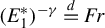 $(E_1^*)^{-\gamma }\overset {d}{=} Fr$
. Then,
$(E_1^*)^{-\gamma }\overset {d}{=} Fr$
. Then,
 $$ \begin{align*} & \dfrac{1}{ F^{-1}\left( 1 - \frac{1}{N} \right)} \left[ \vartheta_{N, N, T}- F^{-1}\left( 1-\dfrac{l}{N} \right)\right] = \dfrac{1}{U_F(N)} \left[ \vartheta_{N, N, T}- U_F\left( \dfrac{N}{l} \right)\right]\\ & \quad= \dfrac{1}{U_F(N)}\vartheta_{N, N, T} - \dfrac{U_F(N \times l^{-1})}{U_F(N)} \Rightarrow Fr -( l^{-1})^{\gamma}= Fr -\dfrac{1}{l^{\gamma}}, \end{align*} $$
since by Corollary 1.2.10 in de Haan and Ferreira (Reference de Haan and Ferreira2006), $U_F(x)\in RV_{\gamma }$
and
$U_F(x)\in RV_{\gamma }$
and $\vartheta _{N, N, T}/U_F(N)\Rightarrow Fr$
by Corollary 1.2.4 in de Haan and Ferreira (Reference de Haan and Ferreira2006).
$\vartheta _{N, N, T}/U_F(N)\Rightarrow Fr$
by Corollary 1.2.4 in de Haan and Ferreira (Reference de Haan and Ferreira2006).
For $\gamma =0$
and let
$\gamma =0$
and let $Gu$
be an RV with
$Gu$
be an RV with $P(Gu\leq x) = \exp (-e^{-x})$
for
$P(Gu\leq x) = \exp (-e^{-x})$
for $x\in {\mathbb {R}}$
; note that
$x\in {\mathbb {R}}$
; note that $-\log (E_1^*)\overset {d}{=}Gu$
. By Corollary 1.2.4 in de Haan and Ferreira (Reference de Haan and Ferreira2006), there exists an
$-\log (E_1^*)\overset {d}{=}Gu$
. By Corollary 1.2.4 in de Haan and Ferreira (Reference de Haan and Ferreira2006), there exists an $\hat {f}(\cdot )$
such that
$\hat {f}(\cdot )$
such that $\alpha _N = \hat {f}(F^{-1}(1-1/N))$
for
$\alpha _N = \hat {f}(F^{-1}(1-1/N))$
for $\alpha _N$
of equation (A.5). For this
$\alpha _N$
of equation (A.5). For this $\hat {f}$
, we have
$\hat {f}$
, we have
 $$ \begin{align*} & \dfrac{1}{\hat{f}\left(F^{-1}\left( 1 - \frac{1}{N} \right)\right)} \left( \vartheta_{N, N, T} - F^{-1}\left( 1 - \frac{l}{N} \right) \right)\\ & \quad= \dfrac{1}{\alpha_N} \left( \vartheta_{N, N, T} - U_F(N)\right) + \dfrac{1}{\alpha_N} \left( U_F\left(\dfrac{N}{l} \right) - U_F(N) \right)\Rightarrow Gu - \log(l), \end{align*} $$
where the first term converges by Corollary 1.2.4 in de Haan and Ferreira (Reference de Haan and Ferreira2006) and the second term by equation (A.5).
For $\gamma <0,$
necessarily
$\gamma <0,$
necessarily $F^{-1}(1) = U_F(\infty )<\infty $
. Let W be an RV with
$F^{-1}(1) = U_F(\infty )<\infty $
. Let W be an RV with $P(W\leq x) = \exp ( -(-x)^{-1/\gamma } )$
for
$P(W\leq x) = \exp ( -(-x)^{-1/\gamma } )$
for $x<0$
and
$x<0$
and $P(W\leq x)=1$
for
$P(W\leq x)=1$
for $x\geq 0$
, note that
$x\geq 0$
, note that $-(E_1^*)^{-\gamma } \overset {d}{=}W$
. Then,
$-(E_1^*)^{-\gamma } \overset {d}{=}W$
. Then,
 $$ \begin{align*} & \dfrac{1}{F^{-1}(1) - F^{-1}\left(1- \frac{1}{N} \right) }\left(\vartheta_{N, N, T} - F^{-1}\left( 1- \frac{l}{N} \right) \right) \nonumber\\ & \quad= \dfrac{1}{U_F(\infty) - U_F(N) }\left(\vartheta_{N, N, T}- U_F(\infty) \right) + \dfrac{U_F(\infty) - U_F(N/l)}{U_F(\infty) - U_F(N)} \Rightarrow W + \frac{1}{l^{\gamma}}, \end{align*} $$
where the first term converges by Corollary 1.2.4 in de Haan and Ferreira (Reference de Haan and Ferreira2006) and $U_F(\infty )-U_F(x)\in RV_\gamma $
by Corollary 1.2.10 in de Haan and Ferreira (Reference de Haan and Ferreira2006).
$U_F(\infty )-U_F(x)\in RV_\gamma $
by Corollary 1.2.10 in de Haan and Ferreira (Reference de Haan and Ferreira2006).
Proof of Lemma 4.2.
Let $\alpha _N$
be as in equation (A.5) and let
$\alpha _N$
be as in equation (A.5) and let $\beta _N = U_F(N)$
. First, we show that for the constants
$\beta _N = U_F(N)$
. First, we show that for the constants $\alpha _N, \beta _N,$
it holds that
$\alpha _N, \beta _N,$
it holds that
 $$ \begin{align} & \begin{pmatrix} \dfrac{\vartheta_{N, N, T}-\beta_N}{\alpha_N}, \dfrac{\vartheta_{N-1, N, T} -\beta_N}{\alpha_N}, \dots, \dfrac{\vartheta_{N-q, N, T} -\beta_N}{\alpha_N} \end{pmatrix} \nonumber\\ & \qquad\qquad\Rightarrow \gamma^{-1}\begin{pmatrix} {(E_1^*)^{-\gamma}-1 }, {(E_1^*+E_2^*)^{-\gamma}-1}, \dots, {(E_1^*+E_2^*+ \dots + E^*_{q+1})^{-\gamma} -1 } \end{pmatrix}. \end{align} $$
Let $E_1, \dots , E_{q+1}$
be IID standard exponential RVs, and
$E_1, \dots , E_{q+1}$
be IID standard exponential RVs, and $E_1^*, \dots , E_{q+1}^*$
another IID set of standard exponential RVs. Observe that
$E_1^*, \dots , E_{q+1}^*$
another IID set of standard exponential RVs. Observe that $ P\left ( U_T\left (1/(1-\exp ({-E_i}))\right )\leq x \right ) = H_T(x).$
Then,
$ P\left ( U_T\left (1/(1-\exp ({-E_i}))\right )\leq x \right ) = H_T(x).$
Then,
 $$ \begin{align*} & (\vartheta_{N, N, T}, \vartheta_{N-1, N, T}, \dots, \vartheta_{N-q, N,T}) \\ &\overset{d}{=} \left( U_T\left(\frac{1}{1-\exp({-E_{1, n}})} \right), U_T\left(\frac{1}{1-\exp{(-E_{2, n})}} \right), \dots, U_T\left(\frac{1}{1-\exp({-E_{q+1, n}}) } \right)\right)\\ &\overset{d}{=} \left( U_T\left(\dfrac{1}{1- \exp\left( {-\frac{E_1^*}{N}}\right)} \right) , U_T\left(\dfrac{1}{1- \exp\left({-\frac{E_1^*}{N} - \frac{E_2^*}{N-1} }\right)} \right) , \dots, \right.\\ & \quad, \dots, \left. U_T\left(\dfrac{1}{1- \exp\left({-\frac{E_1^*}{N} - \frac{E_2^*}{N-1} - \dots - \frac{E_{q+1}^*}{N-q} }\right)} \right) \right), \end{align*} $$
where the second equality follows by the Rényi (Reference Rényi1953) representation of order statistics from an exponential sample (see Expression (1.9) in Rényi, Reference Rényi1953). We conclude that
 $$ \begin{align} & \left(\dfrac{\vartheta_{N, N, T}-\beta_N}{\alpha_N}, \dots, \dfrac{\vartheta_{N-q, N}-\beta_N}{\alpha_N} \right) \nonumber\\ &\overset{d}{=} \begin{pmatrix} \dfrac{U_T\left(\frac{1}{1- \exp\left( {-\frac{E_1^*}{N}}\right)} \right) -\beta_N}{\alpha_N} , \dots, & \dfrac{U_T\left(\frac{1}{1- \exp\left({-\frac{E_1^*}{N} - \frac{E_2^*}{N-1} - \dots - \frac{E_{q+1}^*}{N-q} }\right)} \right)-\beta_N}{\alpha_N} \end{pmatrix}. \end{align} $$
Examine the first coordinate in the above vector:
 $$ \begin{align*} & \dfrac{U_T\left(\frac{1}{1- \exp\left( {-\frac{E_1^*}{N}}\right)} \right) -\beta_N}{\alpha_N} = \dfrac{U_T\left(\frac{N}{N\left( 1- \exp\left( {-\frac{E_1^*}{N}}\right) \right)} \right) -\beta_N}{\alpha_N} \\ & = \dfrac{U_F\left(\frac{N}{N\left( 1- \exp\left( {-\frac{E_1^*}{N}}\right) \right)} \right) -\beta_N}{\alpha_N} + \dfrac{ U_T\left(\frac{N}{N\left(\!1- \exp\left( {-\frac{E_1^*}{N}}\right)\! \right)} \right)- U_F\left(\!\frac{N}{N\left( 1- \exp\left( {-\frac{E_1^*}{N}}\right) \right)} \!\right) }{\alpha_N}. \end{align*} $$
We can rewrite each term in equation (B.2) as above by decomposing it into a $U_F$
a component and a difference term involving
$U_F$
a component and a difference term involving $U_T$
and
$U_T$
and $U_F$
.
$U_F$
.
We separately analyze the two terms. First, by Theorem 2.1.1 in de Haan and Ferreira (Reference de Haan and Ferreira2006),
 $$ \begin{align} \begin{pmatrix} \dfrac{U_F\left(\frac{1}{1- \exp\left( {-\frac{E_1^*}{N}}\right)} \right) -\beta_N}{\alpha_N} , \dots, & \dfrac{U_F\left(\frac{1}{1- \exp\left({-\frac{E_1^*}{N} - \frac{E_2^*}{N-1} - \dots - \frac{E_{q+1}^*}{N-q} }\right)} \right)-\beta_N}{\alpha_N} \end{pmatrix} \nonumber\\ \Rightarrow \gamma^{-1}\begin{pmatrix} {(E_1^*)^{-\gamma}-1 }, {(E_1^*+E_2^*)^{-\gamma}-1}, \dots, {(E_1^*+E_2^*+ \dots + E^*_{q+1})^{-\gamma} -1 } \end{pmatrix}. \end{align} $$
Second, the difference terms converge to zero. We show this for the first term only, the result follows analogously for the other terms. First, write the difference term as
 $$ \begin{align} & \dfrac{ U_T\left(\frac{N}{N\left( 1- \exp\left( {-\frac{E_1^*}{N}}\right) \right)} \right)- U_F\left(\frac{N}{N\left( 1- \exp\left( {-\frac{E_1^*}{N}}\right) \right)} \right) }{\alpha_N} \nonumber\\ & =\dfrac{ U_T\left(\frac{N}{N\left( 1- \exp\left( {-\frac{E_1^*}{N}}\right) \right)} \right)-U_T(N) } {\alpha_N} - \dfrac{U_F\left(\frac{N}{N\left( 1- \exp\left( {-\frac{E_1^*}{N}}\right) \right)} \right) - U_F(N)}{\alpha_N}\\&\quad + \dfrac{U_F(N) - U_T(N)}{\alpha_N}. \nonumber \end{align} $$
We show that the above expression is $o(1)$
in two steps. First, we show that the difference of the first two terms in the above display tends to zero. Define
$o(1)$
in two steps. First, we show that the difference of the first two terms in the above display tends to zero. Define $ \tilde {h}_{N, T}(x) = ( U_T\left (Nx\right )-U_T(N) )/{\alpha _N}$
.
$ \tilde {h}_{N, T}(x) = ( U_T\left (Nx\right )-U_T(N) )/{\alpha _N}$
. $\tilde {h}_{N, T}$
converges pointwise to
$\tilde {h}_{N, T}$
converges pointwise to $\tilde {h}(x)= {(x^{\gamma }-1)}/{\gamma }$
as
$\tilde {h}(x)= {(x^{\gamma }-1)}/{\gamma }$
as $N, T\to \infty $
by Theorem 3.1, Lemma A.1, and equation (A.5) with
$N, T\to \infty $
by Theorem 3.1, Lemma A.1, and equation (A.5) with $U_T$
in place of
$U_T$
in place of $U_F$
. Since the limit is continuous, and
$U_F$
. Since the limit is continuous, and $\tilde {h}_{N, T}(x)$
is monotonic in x, convergence is locally uniform in y (see Section 0.1 in Resnick, Reference Resnick1987). Define
$\tilde {h}_{N, T}(x)$
is monotonic in x, convergence is locally uniform in y (see Section 0.1 in Resnick, Reference Resnick1987). Define $x_N=N(1-\exp ({-E_1^*/N}))$
. Then,
$x_N=N(1-\exp ({-E_1^*/N}))$
. Then, $x_N\to E_1^*$
and
$x_N\to E_1^*$
and $x_N$
is a bounded sequence. Then, as
$x_N$
is a bounded sequence. Then, as $N, T\to \infty ,$
it holds that
$N, T\to \infty ,$
it holds that $\tilde {h}_{N, T}(x_N^{-1})\to \tilde {h}((E_1^*)^{-1})$
(observe that
$\tilde {h}_{N, T}(x_N^{-1})\to \tilde {h}((E_1^*)^{-1})$
(observe that $E_1^*$
does not depend on N or T). Similarly, define
$E_1^*$
does not depend on N or T). Similarly, define $ \tilde {f}_N(x) = ({U_F\left (Nx\right ) - U_F(N)})/{\alpha _N}$
.
$ \tilde {f}_N(x) = ({U_F\left (Nx\right ) - U_F(N)})/{\alpha _N}$
. $\tilde {f}_N(x)$
converges to the same limit
$\tilde {f}_N(x)$
converges to the same limit $\tilde {h}(x)$
by equation (A.5). As
$\tilde {h}(x)$
by equation (A.5). As $\tilde {f}_N(x)$
is monotonic, convergence is also locally uniform in x, so analogously
$\tilde {f}_N(x)$
is monotonic, convergence is also locally uniform in x, so analogously $\tilde {f}_N(x_N^{-1})\to \tilde {h}((E_1^*)^{-1})$
. Thus, the difference between the first two terms in equation (B.4) tends to zero. Second,
$\tilde {f}_N(x_N^{-1})\to \tilde {h}((E_1^*)^{-1})$
. Thus, the difference between the first two terms in equation (B.4) tends to zero. Second, ${(U_F(N) - U_T(N))}/{\alpha _N}=o(1)$
as in the proof of Theorem 3.1 (take
${(U_F(N) - U_T(N))}/{\alpha _N}=o(1)$
as in the proof of Theorem 3.1 (take $\tau =1$
and recall that conditions of Theorem 3.1 are assumed to hold).
$\tau =1$
and recall that conditions of Theorem 3.1 are assumed to hold).
Combining the above argument with equation (B.3), we obtain equation (B.1).
Last, we translate from the constants $(\alpha _N, \beta _N)$
to the constants of the statement of the lemma. We only show this for the first coordinate in equation (B.1), the argument for the other coordinates is identical, and we split the proof by the sign of
$(\alpha _N, \beta _N)$
to the constants of the statement of the lemma. We only show this for the first coordinate in equation (B.1), the argument for the other coordinates is identical, and we split the proof by the sign of $\gamma $
. For
$\gamma $
. For $\gamma <0,$
 $$ \begin{align*} \dfrac{\vartheta_{N, N, T}-U_F(\infty)}{U_F(\infty)-U(N)} = \dfrac{\vartheta_{N, N, T} - \beta_N}{\alpha_N} \dfrac{\alpha_N}{U_F(\infty)-U(N)} -1 \Rightarrow -\dfrac{(E_1^*)^{-\gamma}-1}{\gamma}\times \gamma -1, \end{align*} $$
where the result follows from Lemma 1.2.9 in de Haan and Ferreira (Reference de Haan and Ferreira2006). For $\gamma>0,$
 $$ \begin{align*} \dfrac{\vartheta_{N, N, T}}{U_F(N)} = \dfrac{\vartheta_{N, N, T} - \beta_N}{\alpha_N} \dfrac{\alpha_N}{U_F(N)} +1 \Rightarrow \dfrac{(E_1^*)^{-\gamma}-1}{\gamma}\times \gamma +1 = (E_1^*)^{-\gamma}, \end{align*} $$
where the result follows from Lemma 1.2.9 in de Haan and Ferreira (Reference de Haan and Ferreira2006). For $\gamma =0,$
the constants in the lemma statement are in fact
$\gamma =0,$
the constants in the lemma statement are in fact $\alpha _N, \beta _N$
(Corollary 1.2.4 in de Haan and Ferreira, Reference de Haan and Ferreira2006) We only need to represent
$\alpha _N, \beta _N$
(Corollary 1.2.4 in de Haan and Ferreira, Reference de Haan and Ferreira2006) We only need to represent $((E_1^*)^{-\gamma }-1))/\gamma $
in the form given in the theorem statement. Observe that for
$((E_1^*)^{-\gamma }-1))/\gamma $
in the form given in the theorem statement. Observe that for $x>0 {(x^{-\gamma }-1)}/{\gamma } \to -\log (x)$
as
$x>0 {(x^{-\gamma }-1)}/{\gamma } \to -\log (x)$
as $\gamma \to 0$
(note the minus). The conclusion follows.
$\gamma \to 0$
(note the minus). The conclusion follows.
Proof of Theorem 4.3.
Follows immediately from Lemmas 4.1 and 4.2 and the continuous mapping theorem.
We now turn toward the proof of Theorem 4.4. We begin by computing the order of the difference between the noisy and the noiseless maximum. Define $EA_{N, T} = \max \left \lbrace { T^{-p} \left \lvert {\varepsilon _{1, T}} \right \rvert , \dots , T^{-p} \left \lvert {\varepsilon _{N, T}} \right \rvert } \right \rbrace $
. Since
$EA_{N, T} = \max \left \lbrace { T^{-p} \left \lvert {\varepsilon _{1, T}} \right \rvert , \dots , T^{-p} \left \lvert {\varepsilon _{N, T}} \right \rvert } \right \rbrace $
. Since $\vartheta _{i, T}= \theta _i + T^{-p} \varepsilon _{i, T}$
, the following elementary inequality holds:
$\vartheta _{i, T}= \theta _i + T^{-p} \varepsilon _{i, T}$
, the following elementary inequality holds:
 $$ \begin{align} \theta_{N, N}- EA_N \leq \vartheta_{N, N, T}\leq \theta_{N, N}+ EA_N \text{ or } \left\lvert {\vartheta_{N, N, T} -\theta_{N, N} } \right\rvert \leq EA_{N, T}. \end{align} $$
Lemma B.1.
-
(1) If
$\sup _{T}{\mathbb {E}} \left \lvert {\varepsilon _{i, T}} \right \rvert ^{\beta }<\infty $
for some
$\beta> 0$
, then
$\vartheta _{N, N, T} -\theta _{N, N}$
is
$O_p ( {N^{1/\beta }}/{T^{p}} )$
. -
(2) Let Assumption 3 hold and
$\varepsilon _{i, T}\sim N(\mu _T, \sigma _T^2)$
for all T. Then,
$\vartheta _{N, N, T}-\theta _{N, N}=O_p( \sqrt {\log (N)}/T^p)$
.



Proof. Consider (1), Let $t>0$
. We compare
$t>0$
. We compare $EA_{N, T}$
to
$EA_{N, T}$
to ${N^s}/{T^p}$
for
${N^s}/{T^p}$
for $s\geq 0$
,
$s\geq 0$
,
 $$ \begin{align*} P\left( \dfrac{EA_{N, T}}{N^s/T^p} \geq t\right) & = P\left(\bigcup_{i=1}^N \left\lbrace {\dfrac{1}{T^p}\dfrac{ \left\lvert {\varepsilon_{i, T}} \right\rvert }{N^s/T^p}\geq t } \right\rbrace \right) \leq \sum_{i=1}^NP\left( \dfrac{ \left\lvert {\varepsilon_{i, T}} \right\rvert }{N^s/T^p} \geq t T^p \right)\\ & \leq NP\left( \left\lvert {\varepsilon_{i, T}} \right\rvert \geq t N^s \right)\\ & \leq N \dfrac{ {\mathbb{E}} \left\lvert {\varepsilon_{i, T}} \right\rvert ^{\beta} }{t^{\beta} N^{\beta s} } \leq \dfrac{\sup_T{\mathbb{E}} \left\lvert {\varepsilon_{i, T}} \right\rvert ^{\beta}}{t^{\beta}} N^{1-\beta s}, \end{align*} $$
where we use Markov’s inequality in the penultimate step. Setting $s=1/\beta $
shows that these probabilities are bounded, uniformly in T, hence
$s=1/\beta $
shows that these probabilities are bounded, uniformly in T, hence $EA_{N, T}= O_p\left ( {N^{1/\beta }}/{T^p} \right )$
. The result follows by inequality (B.5).
$EA_{N, T}= O_p\left ( {N^{1/\beta }}/{T^p} \right )$
. The result follows by inequality (B.5).
Consider (2). By Assumption 3, $(\mu _T, \sigma _T^2)$
is a bounded sequence.
$(\mu _T, \sigma _T^2)$
is a bounded sequence. $EA_{N, T}$
is a maximum of independent normal variables of bounded mean and variance. Then,
$EA_{N, T}$
is a maximum of independent normal variables of bounded mean and variance. Then, $EA_{N, T}=O_p\left (\sqrt {\log (N)}/T^p\right )$
. The result then follows by inequality (B.5).
$EA_{N, T}=O_p\left (\sqrt {\log (N)}/T^p\right )$
. The result then follows by inequality (B.5).
Proof of Theorem 4.4.
The proof changes depending on whether $l=0$
or
$l=0$
or $l>0$
. We begin with
$l>0$
. We begin with $l=0$
and
$l=0$
and $\gamma <0$
. Label
$\gamma <0$
. Label
 $$ \begin{align*} J(x) & = P\left( \dfrac{ (E_1^* + \dots + E_{r+1}^*)^{-\gamma} }{(E_1^*+ \dots + E_{q+1}^*)^{-\gamma}-(E_1^*)^{-\gamma} }\leq x \right), J_{N, T}(x)\\ & = P\left(\dfrac{\vartheta_{N-r, N, T} -F^{-1}(1)}{\vartheta_{N-q, N, T} - \vartheta_{N, N, T}} \leq x \right), \end{align*} $$
using notation of Theorem 4.3. Theorem 4.3 shows that $J_N \Rightarrow J$
.
$J_N \Rightarrow J$
.
Add and subtract $F^{-1}(1)$
in
$F^{-1}(1)$
in $L_{b, N, T}$
to obtain
$L_{b, N, T}$
to obtain
 $$ \begin{align*} L_{b, N, T}(x) = \dfrac{1}{\binom{N}{b}}\sum_{s=1}^{\binom{N}{b}} {\mathbb{I}} \left\lbrace { \dfrac{ \vartheta_{b-r, b, T}^{(s)} - F^{-1}(1) }{\vartheta_{b-q, b, T}^{(s)} - \vartheta_{b, b, T}^{(s)} } + \dfrac{ F^{-1}(1) - \vartheta_{N, N, T} }{\vartheta_{b-q, b, T}^{(s)} - \vartheta_{b, b, T}^{(s)} } \leq x } \right\rbrace. \end{align*} $$
Fix an arbitrary $\epsilon>0$
and define the event
$\epsilon>0$
and define the event $ E_{N, T} = \lbrace \lvert ( F^{-1}(1) - \vartheta _{N, N, T}) /(\vartheta _{b-q, b, T}^{(s)} - \vartheta _{b, b, T}^{(s)} ) \rvert \leq \epsilon \rbrace .$
The goal is to show that
$ E_{N, T} = \lbrace \lvert ( F^{-1}(1) - \vartheta _{N, N, T}) /(\vartheta _{b-q, b, T}^{(s)} - \vartheta _{b, b, T}^{(s)} ) \rvert \leq \epsilon \rbrace .$
The goal is to show that $P(E_{N, T})\to 1$
for any
$P(E_{N, T})\to 1$
for any $\varepsilon>0$
as
$\varepsilon>0$
as $N, T\to \infty $
. Write
$N, T\to \infty $
. Write
 $$ \begin{align} \dfrac{ F^{-1}(1) - \vartheta_{N, N, T} }{\vartheta_{b-k, b, T}^{(s)} - \vartheta_{b, b, T}^{(s)} } & = \dfrac{ F^{-1}(1) - \theta_{N, N} }{\vartheta_{b-q, b, T}^{(s)} - \vartheta_{b, b, T}^{(s)} }+ \dfrac{ \theta_{N, N} - \vartheta_{N, N, T} }{ \vartheta_{b-q, b, T}^{(s)} - \vartheta_{b, b, T}^{(s)} }. \end{align} $$
We show that both terms are $o_p(1)$
, which allows us to conclude that
$o_p(1)$
, which allows us to conclude that $P(E_{N, T})\to 1$
. Focus on the first term in equation (B.6). Recall that
$P(E_{N, T})\to 1$
. Focus on the first term in equation (B.6). Recall that $F^{-1}(1)= U_F(\infty )$
and write the term as
$F^{-1}(1)= U_F(\infty )$
and write the term as
 $$ \begin{align*} \dfrac{ F^{-1}(1) - \theta_{N, N} }{\vartheta_{b-q, b, T}^{(s)} - \vartheta_{b, b, T}^{(s)} }= \dfrac{U_F(\infty)- \theta_{N, N} }{ U_F(\infty)-U_F(N) } \dfrac{U_F(\infty)-U_F(b) }{ \vartheta_{b-q, b, T}^{(s)} - \vartheta_{b, b, T}^{(s)} } \dfrac{ U_F(\infty) - U_F(N)}{U_F(\infty)-U_F(b)}. \end{align*} $$
-
(1) The first term is
$O_p(1)$
under Assumption 2 by Corollary 1.2.4 in de Haan and Ferreira (Reference de Haan and Ferreira2006). This term does not depend on T. -
(2) Second term is
$O_p(1)$
by Lemma 4.2. Lemma 4.2 applies to subsample s, since
$(N, T)$
satisfy conditions of Proposition 3.2, and
$b=o(N)$
. -
(3) Last,
$(U_F(\infty )-U_F(t))\in RV_{\gamma }$
by Corollary 1.2.10 in de Haan and Ferreira (Reference de Haan and Ferreira2006). By Proposition 0.5 in Resnick (Reference Resnick1987)
$ {(U_F(\infty )- U_F(xt))}/{(U_F(\infty )- U_F(t))}\to x^{\gamma }$
uniformly on intervals of the form
$(b, \infty )$
. Hence, using
$b= N^m$
,
$m<1, \gamma <0$
, we obtain
$$ \begin{align*} \frac{U_F(\infty)-U_F(N)}{U_F(\infty)-U_F(N^m)} = \frac{U_F(\infty)-U_F((N^{1-m}N^m))}{U_F(\infty)-U_F(N^m)} \sim (N^{1-m})^{\gamma} \to 0. \end{align*} $$
The last term is
$o(1)$
.


Overall, the first term in equation (B.6) is $o_p(1)$
Now, focus on the second term in equation (B.6). Let condition (1) of Proposition 3.2 hold (the proof is analogous if condition (2) holds instead). Since $\sup _T {\mathbb {E}} \left \lvert {\varepsilon _{i, T} } \right \rvert ^{\beta }<\infty $
, by Lemma B.1, we conclude that
$\sup _T {\mathbb {E}} \left \lvert {\varepsilon _{i, T} } \right \rvert ^{\beta }<\infty $
, by Lemma B.1, we conclude that $\theta _{N, N}-\vartheta _{N, N, T} = O_p({N^{1/\beta }}/{T^{p}})$
. By Lemma 4.2,
$\theta _{N, N}-\vartheta _{N, N, T} = O_p({N^{1/\beta }}/{T^{p}})$
. By Lemma 4.2, ${(\vartheta _{b-q, b, T}^{(s)} - \vartheta _{b, b, T}^{(s)}) }/{(U_F(\infty ) - U_F(b))}$
is
${(\vartheta _{b-q, b, T}^{(s)} - \vartheta _{b, b, T}^{(s)}) }/{(U_F(\infty ) - U_F(b))}$
is $O_p(1)$
. In addition, by Corollary 1.2.10 in de Haan and Ferreira (Reference de Haan and Ferreira2006)
$O_p(1)$
. In addition, by Corollary 1.2.10 in de Haan and Ferreira (Reference de Haan and Ferreira2006) ${1}/{(U_F(\infty )-U_F(t))}$
is
${1}/{(U_F(\infty )-U_F(t))}$
is $RV_{-\gamma }$
, so by Lemma A.4, we can write
$RV_{-\gamma }$
, so by Lemma A.4, we can write ${1}/{(U_F(\infty )-U_F(t))} = t^{-\gamma } L(t)$
for some slowly varying L. Since
${1}/{(U_F(\infty )-U_F(t))} = t^{-\gamma } L(t)$
for some slowly varying L. Since $b=N^m$
, we obtain
$b=N^m$
, we obtain
 $$ \begin{align} \dfrac{ \theta_{N, N} - \vartheta_{N, N, T} }{ \vartheta_{b-q, b, T}^{(s)} - \vartheta_{b, b, T}^{(s)} } & = \left( \theta_{N, N} - \vartheta_{N, N, T}\right) \dfrac{ U_F(\infty) - U_F(b)}{ \vartheta_{b-q, b, T}^{(s)} - \vartheta_{b, b, T}^{(s)}} \dfrac{1}{U_F(\infty)- U_F(b)} \nonumber\\ & = O_p\left(\frac{N^{1/\beta}}{T^{p}}\right) O_p\left( N^{-\gamma m} L(N^m) \right). \end{align} $$ $L(N^m)$
diverges at rate slower than any power of
$L(N^m)$
diverges at rate slower than any power of $N^m$
. Then, the expression in (B.7) is
$N^m$
. Then, the expression in (B.7) is $o_p(1)$
if for some
$o_p(1)$
if for some $\kappa>0,$
it holds that
$\kappa>0,$
it holds that $N^{1/\beta -\gamma m+\kappa }{T^{-p}} \to 0$
. However, such a
$N^{1/\beta -\gamma m+\kappa }{T^{-p}} \to 0$
. However, such a $\kappa>0$
exists since assumptions of Proposition 3.2 hold and
$\kappa>0$
exists since assumptions of Proposition 3.2 hold and $\gamma <\gamma m$
.
$\gamma <\gamma m$
.
The remainder of the proof now proceeds as in Politis and Romano (Reference Politis and Romano1994). Define
 $$ \begin{align*} \tilde{L}_{b, N, T} = \dfrac{1}{\binom{N}{b}}\sum_{s=1}^{\binom{N}{b}} {\mathbb{I}} \left\lbrace { \dfrac{ \vartheta_{b, b, T}^{(s)} - U_F(\infty) }{\vartheta_{b-q, b, T}^{(s)} - \vartheta_{b, b, T}^{(s)} } \leq x } \right\rbrace. \end{align*} $$
On the event $E_{N, T}$
, it holds that
$E_{N, T}$
, it holds that $ \tilde {L}_{b, N, T}(x-\epsilon ) \leq L_{b, N, T}(x)\leq \tilde {L}_{b, N, T}(x+\epsilon )$
. Since
$ \tilde {L}_{b, N, T}(x-\epsilon ) \leq L_{b, N, T}(x)\leq \tilde {L}_{b, N, T}(x+\epsilon )$
. Since $P(E_{N, T})\to 1$
, the above also holds with probability approaching one. Observe that
$P(E_{N, T})\to 1$
, the above also holds with probability approaching one. Observe that $ {\mathbb {E}}(\tilde {L}_{n, b}(x)) = J_{b, T}(x) \Rightarrow J(x)$
.
$ {\mathbb {E}}(\tilde {L}_{n, b}(x)) = J_{b, T}(x) \Rightarrow J(x)$
. $\tilde {L}_{b, N, T}$
is a U-statistic of order b with kernel bounded between 0 and 1. By Theorem A on p. 201 in Serfling (Reference Serfling1980) it holds that
$\tilde {L}_{b, N, T}$
is a U-statistic of order b with kernel bounded between 0 and 1. By Theorem A on p. 201 in Serfling (Reference Serfling1980) it holds that $\tilde {L}_{b, N, T}(x) - J_{b, T}(x)\xrightarrow {p} 0$
. Then, as in Politis and Romano (Reference Politis and Romano1994), for any
$\tilde {L}_{b, N, T}(x) - J_{b, T}(x)\xrightarrow {p} 0$
. Then, as in Politis and Romano (Reference Politis and Romano1994), for any $\epsilon>0$
with probability approaching it holds that
$\epsilon>0$
with probability approaching it holds that $ J(x-\epsilon )-\epsilon \leq L_{b, N, T}\leq J(x+\epsilon ) +\epsilon $
. Letting
$ J(x-\epsilon )-\epsilon \leq L_{b, N, T}\leq J(x+\epsilon ) +\epsilon $
. Letting $\epsilon \to 0$
shows that
$\epsilon \to 0$
shows that $L_{b, N, T}(x)\to J(x)$
at all continuity points x of
$L_{b, N, T}(x)\to J(x)$
at all continuity points x of $J(x)$
. This also shows that
$J(x)$
. This also shows that $\hat {c}_{\alpha } = L^{-1}_{b, N, T}(\alpha )\to J^{-1}(\alpha )=c_{\alpha }$
since weak convergence of CDFs is equivalent to weak convergence of quantiles.
$\hat {c}_{\alpha } = L^{-1}_{b, N, T}(\alpha )\to J^{-1}(\alpha )=c_{\alpha }$
since weak convergence of CDFs is equivalent to weak convergence of quantiles.
Now, consider the case of $l>0$
. Add and subtract
$l>0$
. Add and subtract $U_F(b/l)$
in the subsampling estimator:
$U_F(b/l)$
in the subsampling estimator:
 $$ \begin{align*} L_{b, N, T}(x) = \dfrac{1}{\binom{N}{b}}\sum_{s=1}^{\binom{N}{b}} {\mathbb{I}} \left\lbrace { \dfrac{ \vartheta_{b-r, b, T}^{(s)} - U_F(b/l) }{\vartheta_{b-q, b, T}^{(s)} - \vartheta_{b, b, T}^{(s)} } + \dfrac{ U_F(b/l) -\vartheta_{N- {Nl}/{b}, N, T} }{\vartheta_{b-q, b, T}^{(s)} - \vartheta_{b, b, T}^{(s)} } \leq x } \right\rbrace. \end{align*} $$
First, since b satisfies the conditions of Theorem 4.3
 $$ \begin{align*} \dfrac{ \vartheta_{b-r, b, T}^{(s)} - U_F(b/l) }{\vartheta_{b-q, b, T}^{(s)} - \vartheta_{b, b, T}^{(s)} }\Rightarrow \dfrac{ (E_1^*+ \dots + E_{r+1}^*)^{-\gamma} + l^{-\gamma}}{(E_1^*+ \dots + E_{q+1}^*)^{-\gamma}-(E_1^*)^{-\gamma} }. \end{align*} $$
Similarly to the above, fix some $\epsilon>0$
and define the event
$\epsilon>0$
and define the event
 $$ \begin{align} E_{N, T} = \left\lbrace { \left\lvert { \dfrac{ U_F(b/l) - \vartheta_{N- {Nl}/{b}, N, T}}{\vartheta_{b-q, b, T}^{(s)} - \vartheta_{b, b, T}^{(s)} } } \right\rvert \leq \epsilon } \right\rbrace. \end{align} $$
The goal is to show that $P(E_{N, T})\to 1$
for any
$P(E_{N, T})\to 1$
for any $\epsilon>0$
under the assumptions of the theorem, the proof will then proceed as above. We show this separately for different signs of
$\epsilon>0$
under the assumptions of the theorem, the proof will then proceed as above. We show this separately for different signs of $\gamma $
. Let
$\gamma $
. Let $\gamma <0$
and write the expression under the absolute value as
$\gamma <0$
and write the expression under the absolute value as
 $$ \begin{align} \left[ \sqrt{ \frac{Nl}{b} } \frac{U_F(b/l) -\vartheta_{N- {Nl}/{b}, N, T} }{\frac{b}{l}U^{\prime}_F(\frac{b}{l})} \right] \left[ \frac{U_F(\infty)- U_F(b)}{ \vartheta_{b-q, b, T}^{(s)} - \vartheta_{b, b, T}^{(s)}} \right] \left[\frac{ \frac{b}{l}U^{\prime}_F\left(\frac{b}{l}\right) }{\sqrt{\frac{Nl}{b}} (U_F(\infty)-U_F(b))}\right]. \end{align} $$
The first term is $O_p(1)$
by Theorem 3.3 taken with
$O_p(1)$
by Theorem 3.3 taken with $k=Nl/b$
. Conditions of Theorem 3.3 hold, since
$k=Nl/b$
. Conditions of Theorem 3.3 hold, since $k={Nl}/{b}\sim N^{1-m}$
and conditions of Proposition 3.4 are assumed to hold for
$k={Nl}/{b}\sim N^{1-m}$
and conditions of Proposition 3.4 are assumed to hold for $\delta =1-m$
. The second term is
$\delta =1-m$
. The second term is $O_p(1)$
by Lemma 4.2 as the conditions of Proposition 3.2 hold for N (and hence for b). Finally, by Corollary 1.1.14 in de Haan and Ferreira (Reference de Haan and Ferreira2006), under Assumption 4
$O_p(1)$
by Lemma 4.2 as the conditions of Proposition 3.2 hold for N (and hence for b). Finally, by Corollary 1.1.14 in de Haan and Ferreira (Reference de Haan and Ferreira2006), under Assumption 4 ${ ({b}/{l})U^{\prime }_F\left (\frac {b}{l}\right ) }/{ (U_F(\infty )-U_F(b))}\to -\gamma $
. Multiplying this by
${ ({b}/{l})U^{\prime }_F\left (\frac {b}{l}\right ) }/{ (U_F(\infty )-U_F(b))}\to -\gamma $
. Multiplying this by $\left (Nl/b \right )^{-1/2}\to 0$
shows that overall the last term is
$\left (Nl/b \right )^{-1/2}\to 0$
shows that overall the last term is $o(1)$
.
$o(1)$
.
We conclude that overall the expression in equation (B.9) is $o_p(1)$
.
$o_p(1)$
.
For $\gamma>0$
instead write the expression under the absolute value in equation (B.8) as
$\gamma>0$
instead write the expression under the absolute value in equation (B.8) as

The last term is $o(1)$
by Corollary 1.1.12 in de Haan and Ferreira (Reference de Haan and Ferreira2006), other terms are as above.
$o(1)$
by Corollary 1.1.12 in de Haan and Ferreira (Reference de Haan and Ferreira2006), other terms are as above.
For $\gamma =0,$
write the term of interest as
$\gamma =0,$
write the term of interest as
 $$ \begin{align*} \dfrac{ U_F(b/l) -\vartheta_{N-\frac{Nl}{b}, N, T} }{\vartheta_{b-q, b, T}^{(s)} - \vartheta_{b, b, T}^{(s)} } = \left[ \sqrt{ \frac{Nl}{b} } \frac{U_F(b/l) -\vartheta_{N-\frac{Nl}{b}, N, T} }{\frac{b}{l}U^{\prime}_F(\frac{b}{l})} \right]\left[ \frac{ \frac{b}{l}U^{\prime}_F\left(\frac{b}{l}\right) }{ \vartheta_{b-q, b, T}^{(s)} - \vartheta_{b, b, T}^{(s)}} \right]\left[ \frac{ 1 }{\sqrt{\frac{Nl}{b}} }\right]. \end{align*} $$
The first term is $O_p(1)$
as above. The second term is
$O_p(1)$
as above. The second term is $O_p(1)$
by Lemma 4.2 as by Corollaries 1.1.10 and 1.2.4 in de Haan and Ferreira (Reference de Haan and Ferreira2006), under Assumption 4, we may take
$O_p(1)$
by Lemma 4.2 as by Corollaries 1.1.10 and 1.2.4 in de Haan and Ferreira (Reference de Haan and Ferreira2006), under Assumption 4, we may take $\hat {f}\left (U_F(N)\right ) = NU^{\prime }_F(N)$
. Finally, the last term is
$\hat {f}\left (U_F(N)\right ) = NU^{\prime }_F(N)$
. Finally, the last term is $o(1)$
.
$o(1)$
.
Proof of Remark 6.
Let $\gamma>0$
and consider
$\gamma>0$
and consider $\hat {\gamma }_H$
. Under conditions of Theorem 3.1, equation (A.5) holds with
$\hat {\gamma }_H$
. Under conditions of Theorem 3.1, equation (A.5) holds with $U_T$
in place of
$U_T$
in place of $U_F$
. By Lemma 1.2.10 in de Haan and Ferreira (Reference de Haan and Ferreira2006), this convergence is equivalent to
$U_F$
. By Lemma 1.2.10 in de Haan and Ferreira (Reference de Haan and Ferreira2006), this convergence is equivalent to $U_T(tx)/U_T(x)\to x^{\gamma }$
for all
$U_T(tx)/U_T(x)\to x^{\gamma }$
for all $x>0$
. Now, proof of Theorem 3.2.2 in de Haan and Ferreira (Reference de Haan and Ferreira2006) applies with
$x>0$
. Now, proof of Theorem 3.2.2 in de Haan and Ferreira (Reference de Haan and Ferreira2006) applies with $U_T$
in place of
$U_T$
in place of $U_F$
(U in their notation).
$U_F$
(U in their notation).
Consistency of $\hat {\gamma }_{PWM}$
for
$\hat {\gamma }_{PWM}$
for $\gamma <1$
holds by Theorem 3.6.1 in de Haan and Ferreira (Reference de Haan and Ferreira2006) as equation (A.5) holds with
$\gamma <1$
holds by Theorem 3.6.1 in de Haan and Ferreira (Reference de Haan and Ferreira2006) as equation (A.5) holds with $U_T$
in place of
$U_T$
in place of $U_F$
under the conditions of Theorems 3.1 and 3.3.
$U_F$
under the conditions of Theorems 3.1 and 3.3.
B.2 Proof of Theorem 4.5
We begin by establishing several supporting lemmas.
Lemma B.2. Let $U_{1, N}\leq \dots \leq U_{N, N}$
be the order statistics from an IID sample of size N from a Uniform
$U_{1, N}\leq \dots \leq U_{N, N}$
be the order statistics from an IID sample of size N from a Uniform $[0, 1]$
distribution. If
$[0, 1]$
distribution. If $k=o(N), s= \left \lfloor {\sqrt {k}} \right \rfloor $
, and
$k=o(N), s= \left \lfloor {\sqrt {k}} \right \rfloor $
, and $k\to \infty $
, then
$k\to \infty $
, then
 $$ \begin{align*} \begin{pmatrix} \sqrt{k}\left(\frac{N}{k}U_{k+1, N}-1 \right) \\ \sqrt{k}\left(\frac{N}{k+s}U_{k+s+1, N}-1 \right) \end{pmatrix} \Rightarrow N\left(0, \begin{pmatrix} 1 & 1\\ 1 & 1 \end{pmatrix} \right). \end{align*} $$
Proof. By Lemma 2.2.3 in de Haan and Ferreira (Reference de Haan and Ferreira2006), $ \sqrt {k}\left ( \frac {N}{k}U_{k+1, N}-1 \right )\Rightarrow N(0, 1) \equiv Z.$
To show the result, we only need to show that the suitable scaled difference between
$ \sqrt {k}\left ( \frac {N}{k}U_{k+1, N}-1 \right )\Rightarrow N(0, 1) \equiv Z.$
To show the result, we only need to show that the suitable scaled difference between $U_{k+1, N}$
and
$U_{k+1, N}$
and $U_{k+s-1, N}$
converges to zero in probability. Consider
$U_{k+s-1, N}$
converges to zero in probability. Consider
 $$ \begin{align} & \sqrt{k}\left(\dfrac{N}{k+s}U_{k+s+1, N}-1 \right) - \sqrt{k}\left(\dfrac{N}{k}U_{k+1, N}-1 \right) \nonumber\\ & = \sqrt{k}N\left( \dfrac{k}{k} \dfrac{1}{k+s} U_{k+s+1, N} - \dfrac{1}{k} U_{k+1, N} \right) \nonumber \\ & = \dfrac{N}{\sqrt{k}}\left( U_{k+s+1}- U_{k+1} - \dfrac{s}{N+1} - \dfrac{s}{k+s}U_{k+s+1, N} + \dfrac{s}{N+1} \right) \nonumber\\ & = \dfrac{N}{\sqrt{k}}\left( U_{k+s+1}- U_{k+1} - \dfrac{s}{N+1} \right) -\dfrac{N}{\sqrt{k}}\left( \dfrac{s}{k+s}U_{k+s+1, N} - \dfrac{s}{k+s} \dfrac{k+s+1}{N+1} \right) \nonumber\\ & \quad + \dfrac{N}{\sqrt{k}}\left(\dfrac{s}{N+1} - \dfrac{s}{k+s}\dfrac{k+s+1}{N+1} \right). \end{align} $$
We show that each of the terms in the last equality in equation (B.10) is $o_p(1)$
. The last term:
$o_p(1)$
. The last term:
 $$ \begin{align*} \dfrac{N}{\sqrt{k}} \dfrac{s}{N+1}\left(1- \dfrac{k+s+1}{k+s} \right) \sim \dfrac{s}{\sqrt{k}}\left( 1- \dfrac{k+s+1}{k+s} \right) \to 0 \text{ as }s\sim\sqrt{k}, k\to\infty. \end{align*} $$
Consider the first term. A difference of order statistics from the uniform distribution follows a beta distribution: if $p>r$
, then
$p>r$
, then $U_{p, N}-U_{r, N} \sim $
Beta(
$U_{p, N}-U_{r, N} \sim $
Beta( $p-r, N-p+r+1)$
. Let
$p-r, N-p+r+1)$
. Let $\delta>0$
, then
$\delta>0$
, then
 $$ \begin{align*} & P\left( \left\lvert { \dfrac{N}{\sqrt{k}}\left( U_{k+s+1, N}- U_{k+1, N} - \dfrac{s}{N+1} \right)} \right\rvert \geq \delta \right) \\ & = P\left( \left\lvert {\text{Beta}(s, N-s+1) - {\mathbb{E}}\left(\text{Beta}(s, N-s+1) \right) } \right\rvert \geq \dfrac{\sqrt{k}}{N}\delta \right)\\ &\leq \dfrac{ {\mathrm{Var}}(\text{Beta}(s, N-s+1) ) }{\delta^2 {k}/{N^2}} = \dfrac{ \frac{ s(N-s+1)}{(N+1)^2 (N+2)} }{\delta^2 \frac{k}{N^2}} \sim \dfrac{\frac{s}{N^2}}{\delta^2 \frac{k}{N^2}} = \frac{s}{\delta^2 k} \to 0. \end{align*} $$
Last, turn to the second term. Since $U_{k+s+1, N}\sim $
Beta(
$U_{k+s+1, N}\sim $
Beta( $k+s+1, n-k-s$
), for
$k+s+1, n-k-s$
), for $\delta>0,$
we have
$\delta>0,$
we have
 $$ \begin{align*} & P\left( \dfrac{N}{\sqrt{k}} \left\lvert {\dfrac{s}{k+s}U_{k+s+1, N} -\dfrac{s}{k+s}\dfrac{k+s+1}{N+1}} \right\rvert \geq \delta \right) \\ & = P\left( \left\lvert { \text{Beta}(k+s+1, N-k-s) - {\mathbb{E}}\left(\text{Beta}(k+s+1, N-k-s) \right) } \right\rvert \geq \delta \dfrac{\sqrt{k}(k+s) }{Ns} \right)\\ & \leq {\mathrm{Var}}(\text{Beta}(k+s+1, N-k-s) )\dfrac{ N^2s^2}{ \delta^2 k(k+s)^2 } = \dfrac{(k+s+1)(N-k-s) }{(N+1)^2(N+2)}\dfrac{ N^2s^2}{ \delta^2 k(k+s)^2 } \\ & \sim \dfrac{(k+s+1)s^2 }{k(k+s)^2} \sim \dfrac{1}{k+s} \to 0. \end{align*} $$
The assertion of the lemma now follows.
Lemma B.3. Let $\theta $
be sampled IID from F, let Assumption 4 hold. Let
$\theta $
be sampled IID from F, let Assumption 4 hold. Let $k=o(N), k\to \infty , s= \left \lfloor {\sqrt {k}} \right \rfloor $
. Let
$k=o(N), k\to \infty , s= \left \lfloor {\sqrt {k}} \right \rfloor $
. Let $\theta _{N-k, N}, \theta _{N-k-s, N}$
be the order statistics from F. Then, as
$\theta _{N-k, N}, \theta _{N-k-s, N}$
be the order statistics from F. Then, as $N\to \infty $
,
$N\to \infty $
,
 $$ \begin{align*} \sqrt{k} \begin{pmatrix} \dfrac{ \theta_{N-k, N}- U_F\left(\frac{N}{k} \right) }{\frac{N}{k}U_F'\left(\frac{N}{k} \right)} \\ \dfrac{ \theta_{N-k-s, N}- U_F\left(\frac{N}{k+s} \right) }{\frac{N}{k+s}U_F'\left(\frac{N}{k+s} \right)} \end{pmatrix} \Rightarrow N\left(0, \begin{pmatrix} 1 & 1\\ 1 & 1 \end{pmatrix} \right). \end{align*} $$
Proof. We use the Cramer–Wold device together with a technique used by de Haan and Ferreira (Reference de Haan and Ferreira2006) in proving an asymptotic normality result for a single statistic under a von Mises condition (see proof of Theorem 2.2.1 therein). Observe that (in notation of Lemma B.2) $ (\theta _{N-k, N}, \theta _{N-k-s, N})\overset {d}{=} \left (U_F\left (1/{U_{k+1, N}} \right ), U_F\left ( {1}/{U_{k+s+1, N}} \right ) \right ).$
Let
$ (\theta _{N-k, N}, \theta _{N-k-s, N})\overset {d}{=} \left (U_F\left (1/{U_{k+1, N}} \right ), U_F\left ( {1}/{U_{k+s+1, N}} \right ) \right ).$
Let $(c_1, c_2)\in {\mathbb {R}}^2$
and examine
$(c_1, c_2)\in {\mathbb {R}}^2$
and examine
 $$ \begin{align} & c_1\sqrt{k}\dfrac{ \theta_{N-k, N}- U_F\left(\frac{N}{k} \right) }{\frac{N}{k}U_F'\left(\frac{N}{k} \right)} + c_2\sqrt{k}\dfrac{ \theta_{N-k-s, N}- U_F\left(\frac{N}{k+s} \right) }{\frac{N}{k+s}U_F'\left(\frac{N}{k+s} \right)} \nonumber\\ \overset{d}{=} & c_1\sqrt{k}\dfrac{ U_F\left(\frac{N}{k} \frac{k}{N U_{k+1, N}} \right)- U_F\left(\frac{N}{k} \right) }{\frac{N}{k}U_F'\left(\frac{N}{k} \right)} + c_2\sqrt{k}\dfrac{ U_F\left(\frac{N}{k+s} \frac{k+s}{N U_{k+s+1, N}} \right)- U_F\left(\frac{N}{k+s} \right) }{\frac{N}{k+s}U_F'\left(\frac{N}{k+s} \right)} \nonumber\\ = & c_1\sqrt{k}\int_1^{k/(NU_{k+1 N})} \dfrac{U_F'\left( \frac{N}{k}t \right)}{U^{\prime}_F\left(\frac{N}{k} \right)}dt + c_2\sqrt{k}\int_1^{(k+s)/(NU_{k+s+1, N})} \dfrac{U_F'\left( \frac{N}{k+s}t \right)}{U^{\prime}_F\left(\frac{N}{k+s} \right)}dt. \end{align} $$
Under Assumption 4 $U^{\prime }_F\in RV_{\gamma -1}$
by Corollary 1.1.10 in de Haan and Ferreira (Reference de Haan and Ferreira2006) (up to sign). Then, by Potter’s inequalities (Proposition B.1.9 (5) in de Haan and Ferreira, Reference de Haan and Ferreira2006) for any
$U^{\prime }_F\in RV_{\gamma -1}$
by Corollary 1.1.10 in de Haan and Ferreira (Reference de Haan and Ferreira2006) (up to sign). Then, by Potter’s inequalities (Proposition B.1.9 (5) in de Haan and Ferreira, Reference de Haan and Ferreira2006) for any $\varepsilon , \varepsilon '>0$
starting from some
$\varepsilon , \varepsilon '>0$
starting from some $N_0$
for
$N_0$
for $t\geq 1,$
it holds that
$t\geq 1,$
it holds that
 $$ \begin{align*} & (1-\varepsilon) t^{\gamma-1-\varepsilon'} < \dfrac{U_F'\left(\frac{N}{k} t\right)}{U^{\prime}_F\left(\frac{N}{k} \right)}< (1+\varepsilon)t^{\gamma-1+\varepsilon'},\\ & (1-\varepsilon) t^{\gamma-1-\varepsilon'} < \dfrac{U_F'\left(\frac{N}{k+s} t\right)}{U^{\prime}_F\left(\frac{N}{k+s} \right)}< (1+\varepsilon)t^{\gamma-1+\varepsilon'}. \end{align*} $$
Multiplying by $\sqrt {k}$
and taking integrals with limits of integration as in equation (B.11), we obtain for
$\sqrt {k}$
and taking integrals with limits of integration as in equation (B.11), we obtain for $c_1, c_2\geq 0,$
 $$ \begin{align*} & c_1 (1-\varepsilon)\sqrt{k} \dfrac{ \left(\frac{k}{NU_{k+1, N}} \right)^{\gamma-\varepsilon'}-1}{\gamma-\varepsilon'} + c_2 (1-\varepsilon)\sqrt{k} \dfrac{ \left(\frac{k+s}{NU_{k+s+1, N}} \right)^{\gamma-\varepsilon'}-1}{\gamma-\varepsilon'} \\ &\qquad\qquad\quad \leq c_1 \sqrt{k}\dfrac{U_F\left(\frac{1}{U_{k+1, N}} \right)- U_F\left(\frac{N}{k} \right) }{\frac{N}{k}U_F'\left(\frac{N}{k} \right)}+ c_2\sqrt{k}\dfrac{U_F\left(\frac{1}{U_{k+s+1, N}} \right)- U_F\left(\frac{N}{k+s} \right) }{\frac{N}{k}U_F'\left(\frac{N}{k+s} \right)} \\ &\qquad\qquad\quad \leq c_1 (1+\varepsilon)\sqrt{k} \dfrac{ \left(\frac{k}{NU_{k+1, N}} \right)^{\gamma+\varepsilon'}-1}{\gamma+\varepsilon'}+ c_2 (1+\varepsilon)\sqrt{k} \dfrac{ \left(\frac{k+s}{NU_{k+s+1, N}} \right)^{\gamma+\varepsilon'}-1}{\gamma+\varepsilon'}. \end{align*} $$
Similar inequalities apply for different combinations of signs of $c_1, c_2$
, though with
$c_1, c_2$
, though with $(1-\varepsilon )$
replaced by
$(1-\varepsilon )$
replaced by $(1+\varepsilon )$
for the terms with
$(1+\varepsilon )$
for the terms with $c_i<0$
. By Lemma B.2 and the delta method, we get that for any
$c_i<0$
. By Lemma B.2 and the delta method, we get that for any $\varepsilon '>0$
that satisfies
$\varepsilon '>0$
that satisfies $\varepsilon '\neq \pm \gamma $

with convergence being joint for the two vectors. Since $\varepsilon>0$
is arbitrary, we obtain that
$\varepsilon>0$
is arbitrary, we obtain that
 $$ \begin{align*} c_1 \sqrt{k}\frac{ \theta_{N-k, N}- U_F\left(\frac{N}{k} \right) }{\frac{N}{k}U_F'\left(\frac{N}{k} \right)}+ c_2\sqrt{k}\frac{ \theta_{N-k-s, N}- U_F\left(\frac{N}{k+s} \right) }{\frac{N}{k}U_F'\left(\frac{N}{k+s} \right)}\end{align*} $$
has the same asymptotic distribution as
 $$ \begin{align*} c_1 \sqrt{k} \dfrac{ \left(\frac{k}{NU_{k+1, N}} \right)^{\gamma\pm \varepsilon'}-1}{\gamma\pm\varepsilon'}+ c_2 \sqrt{k} \dfrac{ \left(\frac{k+s}{NU_{k+s+1, N}} \right)^{\gamma\pm\varepsilon'}-1}{\gamma\pm\varepsilon'}.\end{align*} $$
Finally, the conclusion of the lemma follows by the Cramer–Wold device.
Proof of Theorem 4.5.
First, we focus on part (1) and establish the result for $\theta $
. Since F is differentiable, so is
$\theta $
. Since F is differentiable, so is $U_F$
, and
$U_F$
, and $ U^{\prime }_F(t) = [{(1-F(U_F(t)))^2}]/[{f(U_F(t))}]$
. Since
$ U^{\prime }_F(t) = [{(1-F(U_F(t)))^2}]/[{f(U_F(t))}]$
. Since $F(U_F(t))$
is monotonic, the monotonicity assumption on f implies that eventually also
$F(U_F(t))$
is monotonic, the monotonicity assumption on f implies that eventually also $U^{\prime }_F$
is non-increasing/non-decreasing. Let
$U^{\prime }_F$
is non-increasing/non-decreasing. Let $s= \left \lfloor {\sqrt {k}} \right \rfloor $
. Recall
$s= \left \lfloor {\sqrt {k}} \right \rfloor $
. Recall $F^{-1}(1-k/N) = U_F(N/k)$
, then
$F^{-1}(1-k/N) = U_F(N/k)$
, then
 $$ \begin{align} \dfrac{\theta_{N-k, N}- F^{-1}\left(1- \frac{k}{N} \right)}{\theta_{N-k, N}-\theta_{N-k-s, N}} = \dfrac{\frac{\sqrt{k}}{\frac{N}{k}U^{\prime}_F(N/k)} \left( \theta_{N-k, N}- U_F(N/k) \right) }{\frac{\sqrt{k}}{\frac{N}{k}U^{\prime}_F(N/k)} \left(\theta_{N-k, N}-\theta_{N-k-s, N} \right) }. \end{align} $$
By Lemma B.3, the numerator weakly converges to $Z\equiv N(0, 1)$
.
$Z\equiv N(0, 1)$
.
We show that the denominator converges to 1 in probability. Rewrite the denominator as
 $$ \begin{align} & \frac{\sqrt{k}}{\frac{N}{k}U^{\prime}_F(N/k)} \left(\theta_{N-k, N}-\theta_{N-k-s, N} \right) \\ &= \frac{\sqrt{k}}{\frac{N}{k}U^{\prime}_F(N/k)} \left(\theta_{N-k, N} -U_F\left(\dfrac{N}{k} \right) \right) - \frac{\sqrt{k}}{\frac{N}{k}U^{\prime}_F(N/k)} \left(\theta_{N-k-s, N} - U_F\left(\dfrac{N}{k+s} \right) \right) \nonumber\\ &\quad + \frac{\sqrt{k}}{\frac{N}{k}U^{\prime}_F(N/k)} \left(U_F\left(\dfrac{N}{k} \right) - U_F\left(\dfrac{N}{k+s} \right) \right).\nonumber \end{align} $$
The second term can be written as
 $$ \begin{align*} & \frac{\sqrt{k}}{\frac{N}{k+s}U^{\prime}_F(N/(k+s))} \left(\theta_{N-k-s, N} - U_F\left(\dfrac{N}{k+s} \right) \right) \dfrac{\frac{N}{k+s}U^{\prime}_F(N/(k+s))}{\frac{N}{k}U^{\prime}_F(N/k)}. \end{align*} $$
By Assumption 4 and Corollary 1.1.10 in de Haan and Ferreira (Reference de Haan and Ferreira2006), ${U^{\prime }_F(tx)}/{U^{\prime }_F}(t) \to x^{\gamma -1}$
as
${U^{\prime }_F(tx)}/{U^{\prime }_F}(t) \to x^{\gamma -1}$
as $t\to \infty $
locally uniformly in
$t\to \infty $
locally uniformly in $(0, \infty )$
. Hence,
$(0, \infty )$
. Hence,
 $$ \begin{align*} \dfrac{\frac{N}{k+s}U^{\prime}_F(N/(k+s))}{\frac{N}{k}U^{\prime}_F(N/k)} = \dfrac{k}{k+s} \dfrac{U^{\prime}_F\left(\frac{N}{k}\frac{k}{k+s}\right)}{U^{\prime}_F\left( \frac{N}{k}\right)} \to 1 {,} \end{align*} $$
since ${k}/{k+s} \to 1$
. Thus, by Lemma B.3,
${k}/{k+s} \to 1$
. Thus, by Lemma B.3,
 $$ \begin{align*} \frac{\sqrt{k}}{\frac{N}{k}U^{\prime}_F(N/k)} \left(\theta_{N-k, N} -U_F\left(\dfrac{N}{k} \right) \right) - \frac{\sqrt{k}}{\frac{N}{k}U^{\prime}_F(N/k)} \left(\theta_{N-k-s, N} - U_F\left(\dfrac{N}{k+s} \right) \right)\xrightarrow{p} 0. \end{align*} $$
Last, we examine the residual. Observe that $U_F'\geq 0$
. First, suppose
$U_F'\geq 0$
. First, suppose $U^{\prime }_F$
is eventually non-increasing, in which case
$U^{\prime }_F$
is eventually non-increasing, in which case
 $$ \begin{align*} \left(U_F\left(\dfrac{N}{k} \right) - U_F\left(\dfrac{N}{k+s} \right) \right) & = \int_{(N/k)\times k/(k+s)}^{N/k} U^{\prime}_F\left(t \right)dt \leq \dfrac{s}{k+s} \frac{N}{k} U^{\prime}_F\left(\dfrac{N}{k} \dfrac{k}{k+s} \right). \end{align*} $$
Using the above expression, we obtain an upper bound for the residual term
 $$ \begin{align*} \frac{\sqrt{k}}{\frac{N}{k}U^{\prime}_F\left(\frac{N}{k} \right)} \left(U_F\left(\dfrac{N}{k} \right) - U_F\left(\dfrac{N}{k+s} \right) \right) & \leq \frac{\sqrt{k}}{\frac{N}{k}U^{\prime}_F\left(\frac{N}{k} \right)} \left( \dfrac{s}{k+s} \frac{N}{k} U^{\prime}_F\left(\dfrac{N}{k} \dfrac{k}{k+s} \right) \right) \\& = \dfrac{\sqrt{k}s}{k+s} \frac{U^{\prime}_F\left(\frac{N}{k} \frac{k}{k+ s} \right) }{U^{\prime}_F\left(\frac{N}{k} \right)} \to 1 \end{align*} $$
since $s= \left \lfloor {\sqrt {k}} \right \rfloor $
and by local uniform convergence of the ratio of
$s= \left \lfloor {\sqrt {k}} \right \rfloor $
and by local uniform convergence of the ratio of $U^{\prime }_F$
. At the same time, since
$U^{\prime }_F$
. At the same time, since $U_F'$
is eventually non-increasing, we obtain a lower bound
$U_F'$
is eventually non-increasing, we obtain a lower bound
 $$ \begin{align*} \int_{(N/k)\times k/(k+s)}^{N/k} U^{\prime}_F\left(t \right)dt \geq \dfrac{s}{k+s} \frac{N}{k} U^{\prime}_F\left(\dfrac{N}{k} \right), \end{align*} $$
which shows that
 $$ \begin{align*} \frac{\sqrt{k}}{\frac{N}{k}U^{\prime}_F\left(\frac{N}{k} \right)} \left(U_F\left(\dfrac{N}{k} \right) - U_F\left(\dfrac{N}{k+s} \right) \right) \geq \dfrac{\sqrt{k}s}{k+s} \to 1. \end{align*} $$
Hence, the residual term converges to 1. If instead $U^{\prime }_F$
is eventually non-decreasing, swap the
$U^{\prime }_F$
is eventually non-decreasing, swap the $N/(k+s)$
and
$N/(k+s)$
and $N/k$
terms.
$N/k$
terms.
By combining the above arguments and equation (B.13), we conclude that the denominator of equation (B.12) converges to 1 i.p. We conclude that
 $$ \begin{align*} \dfrac{\theta_{N-k, N}- U_F(N/k)}{\theta_{N-k, N}-\theta_{N-k-s, N}} \Rightarrow \dfrac{Z}{1}=Z\sim N(0, 1){.} \end{align*} $$
Now, turn to part (2) and consider the noisy estimates $\vartheta _i$
. If the conclusion of Lemma B.3 holds with
$\vartheta _i$
. If the conclusion of Lemma B.3 holds with $\vartheta $
in place of
$\vartheta $
in place of $\theta $
, then the proof of part (1) applies with order statistics of
$\theta $
, then the proof of part (1) applies with order statistics of $\vartheta $
replacing their noiseless counterparts
$\vartheta $
replacing their noiseless counterparts $\theta $
. In light of this, it is sufficient to establish the result of Lemma B.3 for
$\theta $
. In light of this, it is sufficient to establish the result of Lemma B.3 for $\vartheta $
. We proceed similarly to the proof of Theorem 3.3 and we apply the Cramer–Wold device.
$\vartheta $
. We proceed similarly to the proof of Theorem 3.3 and we apply the Cramer–Wold device.
Observe that $ (\vartheta _{N-k, N, T}, \vartheta _{N-k-s, N, T})\overset {d}{=} \left ( U_T(Y_{N-k, N}), U_T(Y_{N-k-s, N})\right ) $
for Y as in the proof of Theorem 3.3. Let
$ (\vartheta _{N-k, N, T}, \vartheta _{N-k-s, N, T})\overset {d}{=} \left ( U_T(Y_{N-k, N}), U_T(Y_{N-k-s, N})\right ) $
for Y as in the proof of Theorem 3.3. Let $c_1, c_2\in {\mathbb {R}}$
. Then, as in equation (A.12),
$c_1, c_2\in {\mathbb {R}}$
. Then, as in equation (A.12),
 $$ \begin{align*} & c_1\sqrt{k}\dfrac{ \vartheta_{N-k, N, T}- U_F\left(\frac{N}{k} \right) }{\frac{N}{k}U_F'\left(\frac{N}{k} \right)} + c_2\sqrt{k}\dfrac{ \vartheta_{N-k-s, N, T}- U_F\left(\frac{N}{k+s} \right) }{\frac{N}{k+s}U_F'\left(\frac{N}{k+s} \right)}\\ \overset{d}{=} & c_1\sqrt{k}\dfrac{ U_F\left(Y_{N-k, N} \right)- U_F\left(\frac{N}{k} \right) }{\frac{N}{k}U_F'\left(\frac{N}{k} \right)} + c_2\sqrt{k}\dfrac{ U_F\left(Y_{N-k-s, N} \right)- U_F\left(\frac{N}{k+s} \right) }{\frac{N}{k+s}U_F'\left(\frac{N}{k+s} \right)} \\ &+ c_1\sqrt{k}\dfrac{ U_T\left(Y_{N-k, N} \right)- U_F\left(Y_{N-k, N} \right) }{\frac{N}{k}U_F'\left(\frac{N}{k} \right)} + c_2\sqrt{k}\dfrac{ U_T\left(Y_{N-k-s, N} \right)- U_F\left(Y_{N-k-s, N} \right) }{\frac{N}{k+s}U_F'\left(\frac{N}{k+s} \right)} \\ \overset{d}{=} & c_1\sqrt{k}\dfrac{ \theta_{N-k, N}- U_F\left(\frac{N}{k} \right) }{\frac{N}{k}U_F'\left(\frac{N}{k} \right)} + c_2\sqrt{k}\dfrac{ \theta_{N-k-s, N}- U_F\left(\frac{N}{k+s} \right) }{\frac{N}{k+s}U_F'\left(\frac{N}{k+s} \right)} \\ &+ c_1\sqrt{k}\dfrac{ U_T\left(Y_{N-k, N} \right)- U_F\left(Y_{N-k, N} \right) }{\frac{N}{k}U_F'\left(\frac{N}{k} \right)} + c_2\sqrt{k}\dfrac{ U_T\left(Y_{N-k-s, N} \right)- U_F\left(Y_{N-k-s, N} \right) }{\frac{N}{k+s}U_F'\left(\frac{N}{k+s} \right)}. \end{align*} $$
The result now follows: the first two terms converge to the desired limit by Lemma B.3; the third and fourth terms converge to zero i.p., this convergence follows as in the proof of Theorem 3.3 applied at k and $k+s$
.
$k+s$
.
SUPPLEMENTARY MATERIAL
Morozov, V. (2025): Supplement to “Inference on Extreme Quantiles of Unobserved Individual Heterogeneity,” Econometric Theory Supplementary Material. To view, please visit: https://doi.org/10.1017/S0266466625100315.
COMPETING INTERESTS STATEMENT
The author declares that they have no conflicts of interest.
FUNDING STATEMENT
This work has received no external funding.


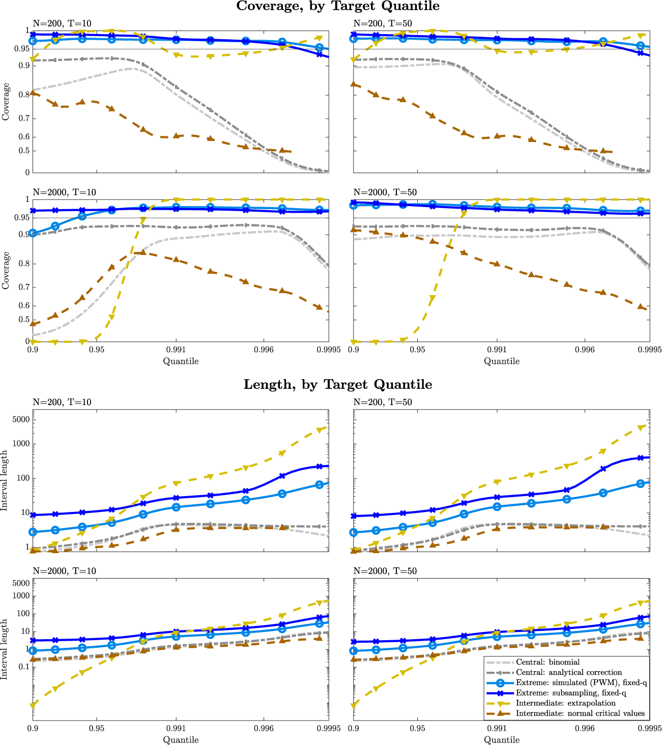


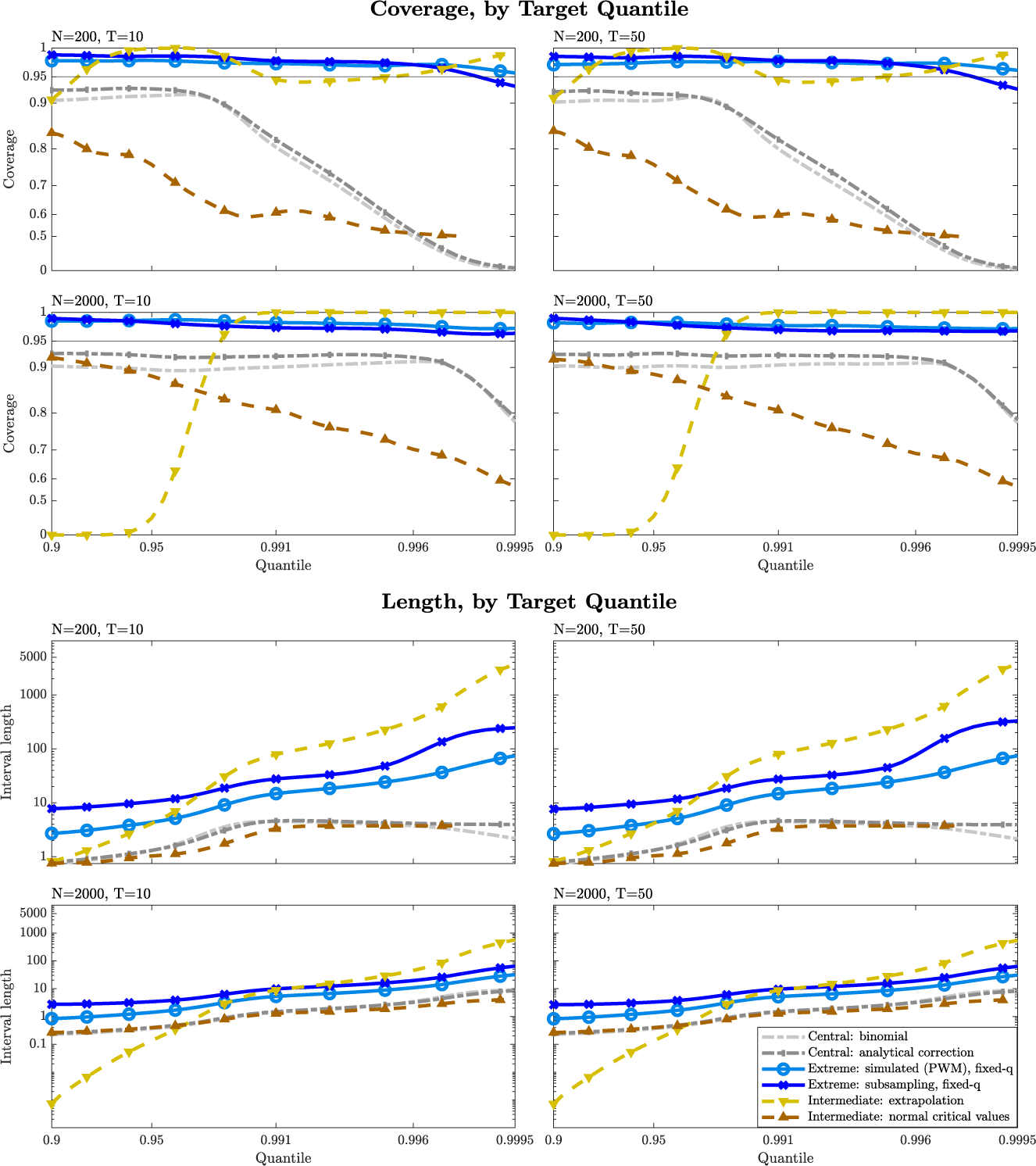

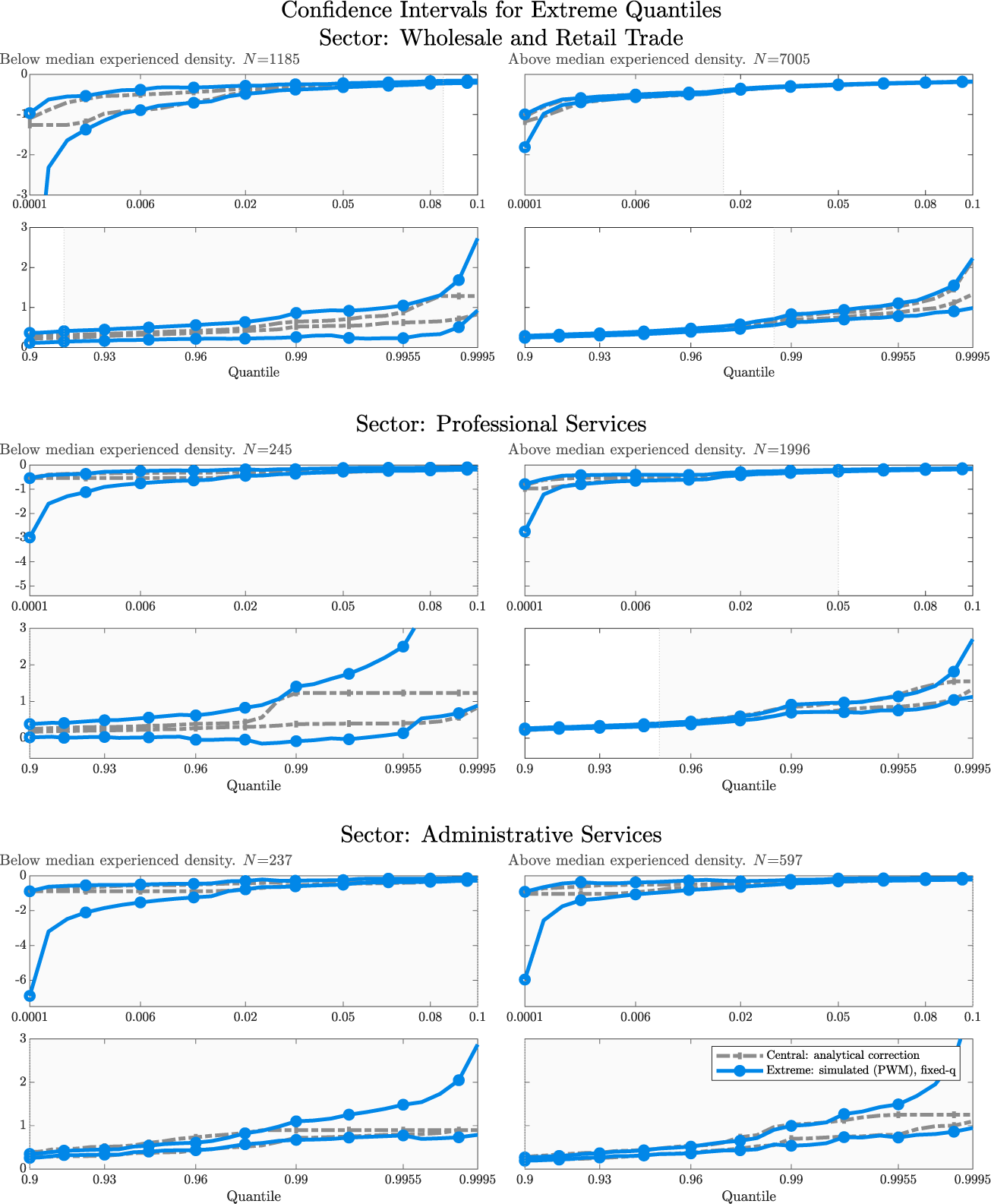

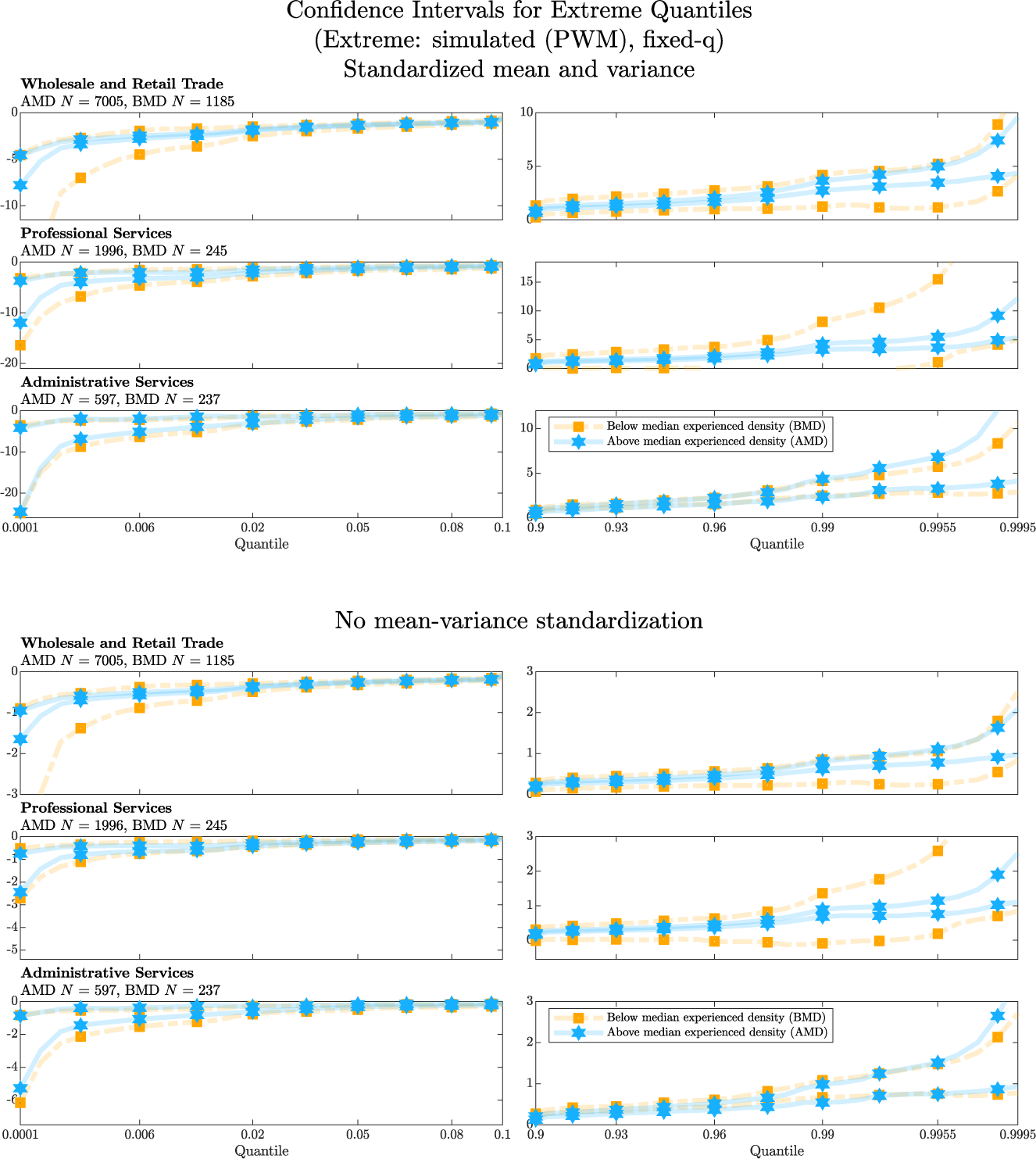


 Open access

