


Introduction
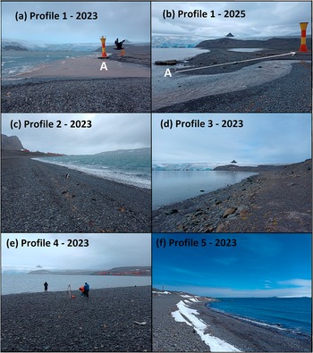
Coastal erosion negatively impacts habitats, biodiversity and infrastructure, and Antarctica is no exception (Bird Reference Bird, Millman and Haq1996, Reid & Massom Reference Reid and Massom2022). Monitoring shoreline changes near Antarctic research infrastructure is crucial for coastal management, risk assessment and decision-making, particularly in this polar setting, where access and logistics are expensive and potentially infrequent. However, reliable data on shoreline changes in the Antarctic are scarce because field surveys are time-consuming, labour-intensive and costly, often being affected by severe weather conditions. Consequently, significant gaps in fundamental historical shoreline data exist. Antarctic research infrastructure (e.g. scientific research stations) provides the best solution to fill knowledge gaps regarding the long-term, in situ monitoring of several parameters, including shoreline variation and its relationships with environmental changes. Research bases and shelters in certain locations, such as Carlini Station in Potter Cove (Fig. 1) on King George Island (Isla 25 de Mayo) - part of the South Shetland Islands, at ~62°14’S and 58°39’W - are significantly affected by coastal erosion, as can be seen in Fig. 2a,b. Coastal erosion is clearly visible on the southern coast of Potter Cove; however, its underlying causes remain unclear. Figure 2 shows five beach locations surveyed in 2023 and 2025. At Site 1 (Fig. 2a,b), the navigational beacon had to be relocated ~37 m landward due to intense coastal erosion. This phenomenon probably results from a combination of factors. These issues include the seasonal variability of sea-ice cover, which modulates coastal exposure to wave energy; wave forcing and associated nearshore currents that drive sediment mobilization and cliff undercutting; precipitation and meltwater runoff that weaken sediment cohesion and promote material transport; freeze-thaw cycles that enhance mechanical weathering of coastal rock; and, to a lesser extent, localized hydrodynamic amplification within coves and embayments. The interactions among these processes create a highly dynamic and spatially heterogeneous erosional environment along the coast of Potter Cove.
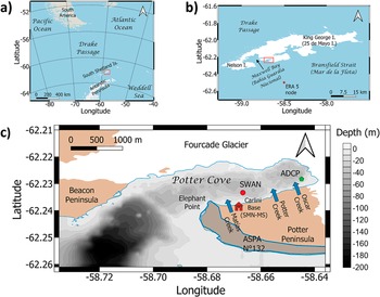
Location of the study area. a. Drake Passage and the South Shetland Islands, Antarctic Peninsula. b. King George Island (Isla 25 de Mayo). c. Potter Cove and Carlini Base. Simulating WAves Nearshore (SWAN) model output locations are indicated by a red circle and the acoustic Doppler current profiler (ADCP) mooring location by a green circle. Blue arrows indicate freshwater inputs from creeks. ASPA = Antarctic Specially Protected Area; SMN-MS = Servicio Meteorológico Nacional meteorological station.

Locations of beach profile surveys conducted in 2023 (a., c.–f.) and 2025 (b.). Profile 1 photographs (a., b.) show the relocation of the navigational beacon caused by shoreline erosion. ‘A’ marks the beacon’s 2023 position.

Coastal erosion is a dynamic process influenced by diverse environmental drivers (Overduin et al. Reference Overduin, Strzelecki, Grigoriev, Couture, Lantuit and St-Hilaire-Gravel2014). Specifically, in Antarctic coves, the interplay between wind and waves, ice cover, sediment transport and precipitation creates a complex environment for studying erosive mechanisms (Lim et al. Reference Lim, Lettmann and Wolff2013). The seasonal variability of sea ice - its presence or absence - modulates the exposure of coastal areas to wave energy, directly affecting the rate and extent of erosion (Barnhart et al. Reference Barnhart, Overeem and Anderson2014). Understanding the processes driving wave-induced erosion in these vulnerable regions is crucial for evaluating the long-term stability of polar coastlines and assessing the broader implications of climate variability on polar ecosystems (Frederick et al. Reference Frederick, Thomas, Bull, Jones and Roberts2016, Korte et al. Reference Korte, Gieschen, Stolle and Goseberg2020).
Sea ice plays a pivotal role in shaping coastal dynamics in Antarctic environments (Massom & Stammerjohn Reference Massom and Stammerjohn2010). Acting as both a protective barrier and a force of erosion, its presence significantly influences the geomorphology of polar shorelines. During the winter months, sea ice shields coastal areas from the direct impacts of ocean waves, mitigating erosion and preserving sedimentary deposits. However, as temperatures rise and sea ice retreats, these coastal zones become vulnerable to wave action and the abrasive effects of drifting ice floes. Moreover, the seasonal freeze-thaw cycles contribute to the mechanical breakdown of coastal rock through frost weathering (Park et al. Reference Park, Kim, Lee and Kim2020). In coves and embayments, where hydrodynamic conditions are intensified, the interplay between sea-ice dynamics and coastal processes is particularly pronounced, often resulting in localized but significant erosional features.
Precipitation, particularly in the form of rain (Vignon et al. Reference Vignon, Roussel, Gorodetskaya, Genthon and Berne2021), influences coastal erosion in Antarctic coves by contributing to surface runoff and soil saturation. This process weakens sediment cohesion and promotes the transport of material into the ocean. Additionally, the freeze-thaw cycles triggered by rainfall and temperature fluctuations can accelerate the mechanical breakdown of coastal rock, amplifying erosion (Trenhaile Reference Trenhaile2014). Only a small number of publications discuss glacial runoff in Antarctica, and even fewer address groundwater flow discharge (Falk & Silva-Busso Reference Falk and Silva-Busso2021). Creeks or meltwater streams (small water discharges that do not form fully developed channels; McKnight & Tate Reference McKnight and Tate1995) could play an important role in coastal erosion in Antarctic coves. These ephemeral flows, often triggered by melting snow or ice, transport sediment and nutrients from higher elevations to the coastline. Over time, they carve shallow channels into the terrain, weakening soil and rock stability and facilitating the movement of material into the ocean. Even though the impact of meltwater streams on coastal erosion is difficult to quantify, their cumulative effect can significantly shape the geomorphology of Antarctic coastal areas, particularly in regions where such flows are recurrent and intensified by seasonal melting (Wright & Thom Reference Wright and Thom2023).
Waves and their associated current systems are the most significant agents driving coastal erosion (Prasad & Kumar Reference Prasad and Kumar2014). Their energy, concentrated along the shoreline, contributes to the mechanical breakdown of rock and the transport of sediment. The erosive power of waves is amplified during storms (Ponti & Guglielmin Reference Ponti and Guglielmin2021) or during ice-free periods, when the absence of a natural buffer allows waves to directly impact the coast. Waves also facilitate the undercutting of cliffs and the redistribution of material, reshaping the coastal landscape over time.
Although coastal erosion in Potter Cove is influenced by multiple processes, wave action may represent a key mechanism for the direct transfer of energy to the shoreline. In contrast to other factors, whose impacts are often gradual or spatially diffuse, waves tend to concentrate mechanical energy at the coast, influencing sediment mobilization, cliff undercutting and episodic erosion during high-energy events. Accordingly, a characterization of wave dynamics is essential for quantifying coastal change in Potter Cove and for assessing the importance of marine forcing relative to other driving processes.
In this context, the present study addresses shoreline retreat along the southern coast of Potter Cove through a detailed analysis of recent shoreline position changes derived from repeated field surveys. This study aims to characterize the magnitude and variability of coastal erosion affecting the cove by quantifying the spatial patterns of shoreline retreat at selected beach sites. Particular attention is paid to the relationship between observed changes in the shoreline and wave-driven processes, providing new insights into the role of wave energy in shaping Antarctic coastal environments, where long-term shoreline data are extremely limited.
To address this limitation, a numerical modelling approach was employed to simulate wave parameters, with particular emphasis given to winter conditions, when direct wave measurements and visual observations are unavailable. In polar and subpolar coastal environments, shoreline dynamics are controlled by a combination of wave climate, seasonal ice cover and local geomorphology, which together regulate the timing and magnitude of erosive processes. In these regions, wave action becomes particularly relevant during periods when sea ice is reduced or absent, allowing oceanic energy to directly interact with the coast. This study hypothesizes that - if the cove is not frozen - winter wave heights (Hs) are significantly greater than those in summer, thereby increasing the potential for coastal erosion in Potter Cove.
Study area
Potter Cove is a small inlet in Maxwell Bay to the south-west of King George Island (Isla 25 de Mayo), part of the South Shetland Islands. This archipelago is separated from the Antarctic Peninsula by the Bransfield Strait (Mar de la Flota; Fig. 1). To the north and east, the retreating tidewater Fourcade Glacier releases ice and sediment-laden meltwater into the cove (Wölfl et al. Reference Wölfl, Lim, Hass, Lindhorst, Tosonotto and Lettmann2014, Reference Wölfl, Wittenberg, Feldens, Hass, Betzler and Kuhn2016). To the south and west, the ice-free coastline is directly exposed to the action of tides and waves. This section of the cove hosts the Argentine Antarctic research station Carlini Base.
Geological context
During the Quaternary glaciations, the glaciers that covered Potter Peninsula carved deep valleys that now form the straits separating the various islands and coves. Potter Cove is therefore a fjord, tributary to Maxwell Bay, ~4.0 km long and 2.5 km wide, with an area of ~7 km2 and a south-west to north-east orientation. The inland of Potter Peninsula consists of Miocene to modern basaltic and andesitic volcanic rocks (Hawkes Reference Hawkes1961, Lindhorst & Schutter Reference Lindhorst and Schutter2014). These rock outcrops are covered and surrounded by glacial deposits, primarily forming basal and frontal moraines (Barton Reference Barton1965).
Within the cove, the coastal morphology is highly irregular, with poorly developed headlands and significantly infilled bays, particularly in the southern and north-western sectors (Heredia Barión et al. Reference Heredia Barión, Lindhorst, Schutter, Falk and Kuhn2019). In contrast, the north-eastern coast is characterized by rocky cliffs, where the sea is in direct contact with the glacier. Beaches are narrow and composed of glacial to paraglacial sediments (Finkl & Makowski Reference Finkl and Makowski2019, Heredia Barión et al. Reference Heredia Barión, Lindhorst, Schutter, Falk and Kuhn2019), which have a direct or indirect glacial origin - as is expected in a coastal system formed on or in proximity to formerly ice-covered terrains. Marine deposits, such as beaches and hooked and compound spits, are widely distributed throughout the island in those areas of the coast that are uncovered by ice, forming complex bay infills such as in Maxwell Bay, east of Carlini Base (Lindhorst & Schutter Reference Lindhorst and Schutter2014).
Carlini Base (known as Jubany Station before 2012) is located on the lower basin of the Matías meltwater stream, over glacial deposits consisting of lower Holocene basal moraines with interstitial ice. This area is a poorly developed headland where a continuous berm is present and an incipient active cliff has formed over these morainic deposits (Heredia Barión et al. Reference Heredia Barión, Lindhorst, Schutter, Falk and Kuhn2019). Fluvioglacial plains, small deltas and marine accumulation terraces are observed adjacent to the modern beach deposits (Lindhorst & Schutter Reference Lindhorst and Schutter2014).
Bathymetry and sediments
Water depths in the cove range from < 60 m in its inner/proximal part to > 100 m in its outer/distal part (Schloss et al. Reference Schloss, Abele, Moreau, Demers, Bers, González and Ferreyra2012), with maximum water depths of 200 m at the south-west extreme (Fig. 1; Wölfl Reference Wölfl, Wittenberg, Feldens, Hass, Betzler and Kuhn2016, Heredia Barión Reference Heredia Barión, Lindhorst, Schutter, Falk and Kuhn2019, Deregibus et al. Reference Deregibus, Quartino, Ruiz Barlett, Zacher and Bartsch2025). The maximum depth in the inner cove reaches 58 m, whereas the crests are shallower than 30 m; towards the outer shelf, the seabed steeply deepens beyond 100 m, before gradually increasing further in depth. The cove has a U-shaped profile, with a gentle southern slope and a steep northern slope. Severe weather events of varying intensity influence the distribution of sediments. Fine sediments (silt and sand) from Fourcade Glacier meltwater and runoff accumulate in the inner and deeper central areas of the cove, transitioning to coarser materials towards the mouth and shore. This would indicate a more protected head and centre, with increasing wave energy towards the fjord and coastline. In contrast, shallow-water areas in the north-west and south-east are composed of stones and boulders covered by macroalgae near slopes and rocky outcrops, far from fine sediment sources (Wölfl et al. Reference Wölfl, Lim, Hass, Lindhorst, Tosonotto and Lettmann2014). Several meltwater streams discharge into the southern coast of the cove (Fig. 1). Varela (Reference Varela1998) studied Matías and Potter creeks, which usually begin flowing in spring. Matías Creek has a mixed snowy-lacustrine regime, whereas Potter Creek, with a snowy-glacial regime, exhibits greater discharge variations.
Climate
Braun et al. (Reference Braun, Esefeld and Peter2017) characterized the region’s climate as relatively mild, humid (~700 mm annual precipitation) and dominated by strong westerly winds, which are associated with warm, humid conditions, in contrast to colder conditions under easterly winds (Klöser et al. Reference Klöser, Ferreyra, Schloss, Mercuri, Laturnus and Curtosi1994, Roese & Drabble Reference Roese and Drabble1998, Schloss et al. Reference Schloss, Abele, Moreau, Demers, Bers, González and Ferreyra2012). Studies have reported rising air temperatures at Carlini Base, with more pronounced warming in autumn (0.54°C per decade) and winter (0.38°C per decade) from 1987 to 2022 (Schloss et al. Reference Schloss, Abele, Moreau, Demers, Bers, González and Ferreyra2012, Deregibus et al. Reference Deregibus, Quartino, Ruiz Barlett, Zacher and Bartsch2025). Similar trends were observed at other stations on King George Island (Ferron et al. Reference Ferron, Simões, Aquino and Setzer2004). Schloss et al. (Reference Schloss, Abele, Moreau, Demers, Bers, González and Ferreyra2012) linked increasing air temperatures (1991–2009) to warmer surface waters, reduced salinity and higher total suspended particulate matter during winter, suggesting an influx of warm, particle-laden freshwater from glacial melting.
Sea-ice dynamics
Historically, the sea surface at Potter Cove froze each winter, forming an ice pack ~1 m thick, while drifting ice would dominate the rest of the year (Roese & Drabble Reference Roese and Drabble1998). Between 1991 and 2009, sea ice covered at least 15% of the cove for an average of 215 days (late April to late November), with little interannual variability (Schloss et al. Reference Schloss, Abele, Moreau, Demers, Bers, González and Ferreyra2012). However, in recent decades, sea-ice extent and thickness have declined due to warmer winters and springs, with there being several consecutive years during which the ice pack failed to consolidate or even form, especially in the period from 2010 and 2016 (Ruiz Barlett et al. Reference Ruiz Barlett, Sierra, Costa and Tosonotto2021). Deregibus et al. (Reference Deregibus, Quartino, Ruiz Barlett, Zacher and Bartsch2025) found an inverse relationship between mean annual air temperature and fast-ice duration, which ranged from 14 to 134 days between 2009 and 2019. Air temperature increases were more pronounced in all seasons from 2013 to 2022, with a sharp decline in ice cover since 2015, mirroring trends along the West Antarctic Peninsula.
In the outer sector of the Cove - corresponding to the area analysed by Ruiz Barlett et al. (Reference Ruiz Barlett, Sierra, Costa and Tosonotto2021) - surface ice cover was estimated from MERRA-2 (Modern-Era Retrospective analysis for Research and Applications) reanalysis data (Gelaro et al., Reference Gelaro, McCarty, Suárez, Todling, Molod and Takacs2017; spatial resolution 0.500° × 0.625°) for the period 1980–2025. The record exhibits a pronounced seasonal cycle, with higher ice concentrations occurring predominantly during the winter months and very low or negligible values recorded during summer. The winter ice cover does not persist uniformly from year to year; instead, it shows marked interannual variability, with some winters characterized by extensive ice coverage (frequently exceeding moderate to high concentration levels), whereas other winters displayed reduced or more fragmented ice conditions. Overall, the ice regime is highly variable in both timing and magnitude, indicating that periods of substantial ice cover are intermittent rather than continuous over the study period. In the most recent years of the record, surface ice cover appears to be less extensive and less persistent during the winter, with generally lower peak concentrations and shorter ice-covered periods compared to some earlier intervals.
Tidal regime, wind-driven circulation and waves
Dragani et al. (Reference Dragani, Drabble, D’Onofrio and Mazio2004, Reference Dragani, D’Onofrio, Speroni, Fiore and Borjas2005) presented a description of the tidal dynamics in Bransfield Strait. The tides in this region are mixed, with a predominant semi-diurnal component. In Potter Cove, mean tidal amplitudes reach 1.48 m during spring tides and 1.20 m during neap tides (Schöne et al. Reference Schöne, Pohl, Zakrajsek and Schenke1998). Roese & Drabble (Reference Roese and Drabble1998) reported very weak currents in the cove, averaging up to 0.04 m s−1. However, wind plays a more significant role in circulation than tides (Lim et al. Reference Lim, Lettmann and Wolff2013, Lim Reference Lim2014). Two wind-driven circulation patterns - a cyclonic gyre for westerly and easterly winds up to 5 m s−1 and a vertical cell with surface currents - aligned with the wind direction, while deep currents move oppositely, causing downwelling or upwelling in the inner cove depending on wind direction (Roese & Drabble, Reference Roese and Drabble1998).
Waves in the inner cove are slight, except under northern and north-western winds, whereas more significant wave activity occurs in the outer cove. During October–November 1993, visual observations of waves were carried out and maximum Hs of between 0.3 and 0.9 m along the southern coast were reported, extending from Profile 1 (P1) to P5 (Fig. 3). Based on a numerical investigation, Lim (Reference Lim2014) found that significant Hs in the inner Potter Cove are ~40–50% smaller than those near its mouth. Additionally, wave-induced bed shear stress is suggested to be a major driving force behind bed sediment erosion, especially in shallow water regions.
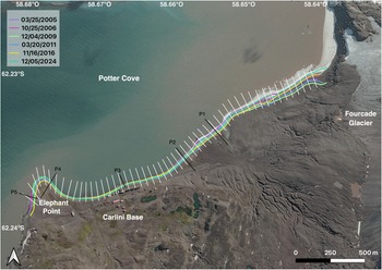
Shorelines manually digitized in Google Earth Pro for different years, with shore-normal transects generated using the Digital Shoreline Analysis System (DSAS) version 6 (white). In situ beach profiles are shown in black. P = Profile.

Data
Satellite imagery - a widely used tool for monitoring the evolution of coastal areas (Vitousek et al. Reference Vitousek, Buscombe, Vos, Barnard, Ritchie and Warrick2023) - along with in situ beach profiling and sedimentological characteristics were used in this study to investigate shoreline position changes along the period 2005–2024. Wind and wave data, as well as wave parameters from global and local models, were analysed to characterize one of the possible erosion drivers in the Potter Cove.
Satellite imagery
Google Earth Pro (GEP) provides free high-resolution images, making it an increasingly valuable tool for research (Warnasuriya et al. Reference Warnasuriya, Kumara, Gunasekara, Gunaalan and Jayathilaka2020). The Digital Shoreline Analysis System (DSAS) version 6 (Himmelstoss et al. Reference Himmelstoss, Henderson, Farris, Kratzmann, Bartlett and Ergul2024) is a standalone application that calculates shoreline or boundary change over time. DSAS enables the user to calculate rate-of-change statistics from multiple historical shoreline positions. It also provides an automated method for establishing measurement transects, performs rate calculations and provides uncertainties associated with rates of change. A user-friendly interface allows the user to complete the workflow for shoreline change analysis. A total of six satellite images acquired between 2005 and 2024 were used in this study.
Beach profiles
In Antarctica, beach profile surveys can only be conducted when the coastline is ice-free and accessible and weather conditions allow safe field operations. The persistence of sea ice and severe meteorological constraints render direct coastal monitoring logistically infeasible and are widely recognized in Antarctic coastal research, where summer-based campaigns remain the standard approach for documenting shoreline and morphodynamic processes.
In situ beach profiles were measured during the summer seasons of 2020, 2023 and 2025 at five locations along the southern coast of Potter Cove. P1 and P2 were located to the east of Carlini Base (Figs 1, 2a–c & 3), in the direction of the glacier, and were referenced from fixed metal stakes. P3 was measured at Carlini Base (Figs 1, 2d & 3), using the tidal benchmark of the Argentine Naval Hydrographic Service (Servicio de Hidrografía Naval, SHN), which is located 7.883 m above mean sea level (MSL). P4 and P5 were situated at Elephant Point, with P4 orientated towards the interior of the cove and P5 facing the open sea (Figs 1, 2e,f & 3). The fixed reference points for these two profiles were based on the infrastructure of the station’s helipad.
All surveys were conducted during low tide and under calm wind conditions, allowing measurements down to ~1 m water depth. Elevation data were collected using precise differential levelling along cross-shore transects. The elevation measurements were referenced to MSL by determining the vertical offset between the fixed profile benchmarks and the SHN tidal benchmark. This was accomplished using a Global Navigation Satellite System (GNSS) real-time kinematic (RTK) system to accurately measure the relative elevation between the fixed points and the tidal benchmark. Once referred to MSL, all profiles were then interpolated horizontally to provide elevation data every 5 m along each transect.
Beach slope was calculated from the portion of each profile corresponding to the active beach zone, defined as the area between the Mean Higher-High Water and the Mean Lower-Low Water tidal levels, obtained from tide tables provided by SHN (https://www.hidro.gov.ar/oceanografia/tmareas/Form_TMareas.asp?op=2). This section represents the morphodynamically active zone, which is subject to regular wave and tidal processes. The volume of sediment within each profile was estimated using the trapezoidal integration method over the entire interpolated profile.
Sediments
Sediment samples were collected and analysed at the same sites where beach profiles were measured (Fig. 3). Grain-size analyses were performed using nine sieves, ranging from −4 to +4 phi, mounted on a mechanical Ro-Tap mechanical sieve shaker. The morphological interpretation of the study area was based on Google Earth and Bing Map satellite images, together with the available geomorphological maps published by Heredia Barión et al. (Reference Heredia Barión, Lindhorst, Schutter, Falk and Kuhn2019).
Wind
Wind speed and direction were measured every 3 h at a meteorological station located adjacent to Carlini Base (Fig. 1), with sensors installed at a height of 11 m. This station, known as Jubany, is maintained by the Argentine National Meteorological Service (Servicio Meteorológico Nacional, SMN; https://www.smn.gob.ar/). ERA5 reanalysis data (Hersbach et al. Reference Hersbach, Bell, Berrisford, Hirahara, Horanyi and Munoz-Sabater2020; https://cds.climate.copernicus.eu/datasets) were used to drive the nested wave model system implemented in this study.
Waves
The ERA5 dataset was used to describe the seasonal wave climate outside the Cove (https://www.ecmwf.int/en/forecasts/datasets/reanalysis-datasets/era5). This represented the fifth-generation European Centre for Medium-Range Weather Forecasts (ECMWF) reanalysis of the global climate and weather for recent decades. The ocean wave model used in ERA5 is WAM (The Wamdi Group 1988). Data are gridded to a regular grid of 0.5° for the ocean waves with 1 h time steps.
The only long-term in situ observations of directional waves available for Potter Cove were collected between 2012 and 2015 using an Aanderaa RDCP 600 acoustic Doppler current profiler (ADCP) moored at the north-eastern extreme of the cove, close to the glacier front (Fig. 1). The instrument was configured to record a set of wave parameters every 30 min. Although the primary objective of the deployment was to measure currents as part of a project on glacier retreat, wave data were also acquired. Due to the instrument’s location (relatively sheltered from the more energetic wave systems arriving from the north-west and north-east), the recorded wave energy values primarily represent the lowest levels relative to the rest of Potter Cove. Breaker heights were visually observed from the beach at Carlini Base twice daily during the summer seasons of 2022–2023 and 2024–2025 (Fig. 1). Observations followed the methodology established by the Littoral Environment Observation (LEO) Data Collection Program (Schneider Reference Schneider1981), whereby the observer estimates the height of the breakers at the most seaward line, which typically represents the largest waves. In Potter Cove, breakers are generally small and occur relatively close to shore, making visual estimation feasible and reliable. Based on the data collected during both summers, breaker heights were generally less than 0.5 m.
Methodology
This section outlines the methodology employed to determine shoreline changes using satellite imagery, along with the modelling framework developed to simulate wave dynamics within Potter Cove. This integrated approach combines remote sensing analysis with numerical simulations, providing a robust foundation for understanding the coastal processes at play.
Satellite shoreline position
The methodology proposed by Warnasuriya et al. (Reference Warnasuriya, Kumara, Gunasekara, Gunaalan and Jayathilaka2020) to obtain shoreline positions from GEP satellite imagery and to analyse shoreline variation using the DSAS v6.0.168 tool (Himmelstoss et al. Reference Himmelstoss, Henderson, Farris, Kratzmann, Bartlett and Ergul2024) was used in this study. To compute the changes in the shoreline, DSAS requires two key inputs: shoreline position and a baseline. High-resolution satellite images (0.31–1.84 m) from various sources available on GEP were used to delineate the land-water boundary of the study site corresponding to the instantaneous shoreline (ISL). ISLs were manually digitized using the Path tool at a constant eye altitude of 300 m. To ensure consistency, the tilt of satellite images was maintained at 0° by activating the ‘Do not automatically tilt while zooming’ option in GEP. ISLs were saved in KML (Keyhole Markup Language) format and later converted to GeoJSON using QGIS 3.4. All ISLs were projected using the WGS84 UTM (Universal Transverse Mercator) coordinate system.
A positional shift was observed in historical satellite images when compared to the 2024 reference image, using the rooftops of buildings at Carlini Base as a control reference. To quantify this shift, five ground control transects were selected (P1 to P5; Fig. 3), and the displacements (x, y) were estimated in terms of distance (d) and direction (α). A correction was applied to all ISLs using the ‘Field Calculator’ in QGIS, adjusting the shoreline positions according to Equations 1 & 2:
 $$\begin{align}x = d\sin(\alpha) \end{align}$$
 $$\begin{align}y = d\cos(\alpha) \end{align}$$
For the analysis of the changes, each shoreline must have an associated positional uncertainty. The total uncertainty was estimated as the sum of the digitizing error (DE), tidal error (TE) and shifting error (SE; Warnasuriya et al. Reference Warnasuriya, Kumara, Gunasekara, Gunaalan and Jayathilaka2020). The DE was assessed considering the manual delineation of the land-water boundary at a constant eye altitude (300 m), which has been shown to minimize variability in shoreline tracing. The TE was approximated using the tidal range at the time of image acquisition and the mean beach slope, where horizontal displacement is derived from the product of tidal amplitude and beach slope angle. The SE corresponds to minor georeferencing discrepancies between images, evaluated through stable ground control features (building rooftops) common to all dates. The baseline was carefully designed to ensure that all appended shorelines were intersected at nearly uniform intervals. Transects were cast at 100 m intervals, with a smoothing distance of 500 m, and each transect extended 300 m seaward (Fig. 3). These transects intersected each shoreline to generate measurement points, which were subsequently used to calculate shoreline change rates. The DSAS provides various rate-of-change statistics to analyse shoreline dynamics. Among them, the net shoreline movement (NSM) measures the total distance between the oldest and the most recent shoreline for each transect, expressed in metres, and the linear regression rate (LRR) determines the rate of shoreline change by fitting a least-squares regression line through all shoreline positions along a transect, ensuring that the sum of squared residuals is minimized.
Wave modelling
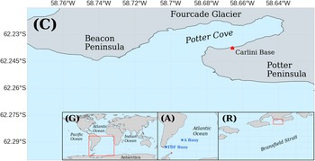
Wind wave parameters in Potter Cove were simulated using a set of nested computational grids: G (global), A (Atlantic), R (regional) and C (cove). The Wavewatch III model (WW3 model; https://polar.ncep.noaa.gov/waves/wavewatch/) was implemented in the G, A and R grids, whereas the Simulating WAves Nearshore model (SWAN model; https://swanmodel.sourceforge.io/) was used in the C grid. The SWAN model was forced at its open boundaries using wave spectra provided by the WW3 model. All the computational grids are detailed in Fig. 4. The G grid covers the area from 85°S to 85°N, with a spatial resolution of 2° in longitude and 1° in latitude and a time step of 600 s. The A grid extends from 74°S to the Equator and from 80°W to 14°E, with a 0.5° spatial resolution in both directions and a time step of 450 s. The R grid spans from 62.1°S to 62.9°S and from 58.1°W to 59.7°W, with a resolution of 0.02° and a time step of 50 s.
Sea-level variations (TPXO Global Tidal Models, 0.4° × 0.4° resolution; https://www.tpxo.net/global) were implemented in grids G and A. Ocean currents from the Global Ocean Physics Analysis and Forecast (https://data.marine.copernicus.eu/products) and GOFS 3.1 (https://www.hycom.org/dataserver/gofs-3pt1/analysis), 1/12° × 1/12° resolution, were implemented in grids G, A and R. Surface winds from ERA5 (see earlier) were used as forcing for the WW3 model in grids G, A and R and for the SWAN model in grid C. Bathymetric data for G, A and R grids were obtained from the Gridded Bathymetry Data with a 15 arc-second interval (https://www.gebco.net/data_and_products/gridded_bathymetry_data/).
Computational domains used for the wave models: Global (G), Atlantic (A), Regional (R) and Potter Cove (C). Wave buoy observations used for model validation in the G and A domains are indicated by blue stars. TDF = Tierra del Fuego.

Simulated wave parameters in the A grid were validated against wave observations from two buoys. One of them was a directional wave recorder (Datawell Waverider) deployed at 53.66°S, 67.30°W between January 1998 and March 1999 on the continental shelf off Tierra del Fuego at a depth of 66 m. It was configured to measure 20 min wave records with a 0.5 s sampling interval every 3 h. The root-mean-square error (0.33 m), correlation coefficient (0.88) and bias (0.14 m) between the observed and simulated Hs indicate a very good performance of the wave model over the austral continental shelf of South America. The other buoy was a 3 m-diameter instrument (https://oceanobservatories.org/) deployed at ~4500 m depth at 42.92°S, 42.43°W. Its data were analysed for the periods from October 2016 to January 2018. This buoy had a Triaxys directional accelerometer package onboard. The wave model showed very good performance in the south-western South Atlantic Ocean, as evidenced by the root-mean-square error (0.46 m), correlation coefficient (0.9) and bias (−0.11 m) obtained from the comparison between observations and simulations.
The high-resolution C grid for Potter Cove spans from 62.22°S to 62.30°S and from 58.62°W to 58.78°W, comprising 128 × 68 nodes, with a spatial resolution of 0.00125° in longitude (124 m) and latitude (74 m) and a time step of 60 s. The SWAN model was configured to compute directional spectra using 36 directions (10° apart) over a frequency range from 0.0521 (19.91 s) to 1 Hz (1 s), discretized into 31 frequencies. This maximum wave period was considered appropriate to capture the weak swell conditions in the Cove. All relevant wave processes were included: depth-induced breaking (BREA), triad wave-wave interactions (TRIAD), quadruplet wave-wave interactions (QUAD), whitecapping (WCAP), bottom friction (FRIC) and diffraction (DIFFRAC), using default model parameters. Model results for the C grid were compared with visual wave observations collected from the coastline of Potter Cove during January and February 2023. The wave model showed a good performance, as evidenced by the root-mean-square error (0.15 m), correlation coefficient (0.87) and bias (−0.13 m) obtained from the comparison between observed and simulated Hs.
Tidal sea level from TPXO Global Tidal Models was included as a forcing in the C grid and was previously validated against local observations, showing very good agreement. Currents were not included in the SWAN model forcing due to their low magnitude within the Cove (mean currents below 0.20 m s−1; Roese & Drabble Reference Roese and Drabble1998) and the low resolution of the current product used to cover the area. ERA5 surface wind data failed to adequately represent wind intensity and direction in the Cove; therefore, hourly in situ wind data from the SMN meteorological station (Fig. 1) were used to force the SWAN model, assuming spatial homogeneity over the small C grid. The bathymetry of Potter Cove was represented by combining the Gridded Bathymetry Data with depth measurements from a local bathymetric survey.
Beach profiles and sediment analysis
Beach profiles were measured using an optical level and a graduated staff, yielding elevation measurements relative to a fixed vertical reference point along transects transverse to the coastline. The quantitative values of coastal erosion or accretion were determined by comparing the horizontal position of each geomorphological feature in the different years of analysis: 2020, 2023 and 2025. In the case of profiles P1, P3 and P5, the base of the active cliff was used as the reference morphological feature, whereas for profiles P2 and P4 the stable berm was employed. The resulting elevation-distance profiles were integrated to compute cross-sectional areas, which represent sediment volumes per unit alongshore length (m3 m−1). Temporal differences in these areas were used to quantitatively assess net sediment gain or loss between survey periods. Sediments from berm, shoreface and backshore environments along the southern coast of the cove were analysed following the classic Folk classification (Folk Reference Folk1954, Reference Folk1974).
Results
To investigate shoreline position changes, a comprehensive analysis was conducted using satellite imagery, in situ beach profiling and sedimentological data. Wind and wave conditions - along with wave parameters derived from both global and local models - were examined to assess possible drivers of coastal erosion in Potter Cove. Offshore Hs conditions were evaluated using ERA5 reanalysis data for the period 2020–2024. Based on this dataset, two high-energy events were identified and subsequently simulated using the numerical modelling framework described earlier.
Satellite analysis
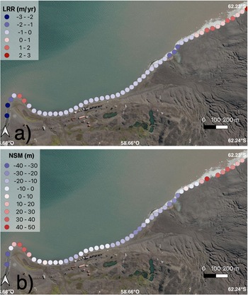
Based on six optical satellite images corresponding to the years 2005, 2006, 2009, 2011, 2016 and 2024, shoreline change rates were calculated using DSAS. Approximately 74% of the analysed coastline has been eroded (Fig. 5), with trends reaching up to −2.6 m year−1, while the remaining transects showed accretion trends with maximum values of 2.5 m year−1. In general, this positive trend is observed in the eastern part of the study area, particularly between the glacier and Potter Creek, where the NSM reaches a maximum of 60 m. To the west, the trend changes towards erosion, with maximum erosion rates of −1.5 m year−1, gradually decreasing towards the beach area where Carlini Base is located. In this sector, erosion remains below −1 m year−1, with an NSM of up to −14 m. To the west of Carlini Base, in the eastern sector of Elephant Point, the trend is positive, with accretion rates above 1 m year−1 and NSM up to 40 m. However, beyond Elephant Point, along the coastal offshore sector, the trend is erosive, with rates of approximately −2.5 m year−1 and a NSM reaching −35 m.
Beach profiles and sediment characterization
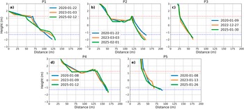
The coastal profiles surveyed in 2020, 2023 and 2025 exhibit contrasting morphodynamic patterns (Fig. 6). In P1 (Figs 2a,b & 6a), a total berm retreat of 20 m was observed: 6 m between 2020 and 2023 and an additional 14 m section by 2025. This retreat was accompanied by a net sediment loss of 5 m3. The beach slope remained relatively stable, with an average of 0.04 ± 0.004, and the profile retained a convex shape throughout the study period, which is characteristic of a reflective beach. A more moderate retreat was recorded in P2 (Figs 2c & 6b), where the berm shifted landward by 3 m over the 5 year period. Despite the smaller horizontal change, this site experienced a much larger sediment loss, totalling 31 m3. Similar to P1, the beach slope was stable (0.04 ± 0.004), and the convex morphology persisted, also suggesting reflective conditions.
P3 (Figs 2d & 6c) displayed a distinctive geomorphological configuration, consisting of a palaeo-scarp, an accumulation platform and a currently active cliff. Here, a subtle landward retreat of the cliff face was noted. Although morphologically more complex, the net volume loss was modest (2 m3), and the average slope (0.08 ± 0.0009) showed no significant variations during the study period. In contrast, P4 (Figs 2e & 6d) revealed a seaward progradation of the berm by 8 m, indicating a depositional trend. The profile evolved from a slightly convex shape in 2020 and 2023 to a slightly concave form in 2025. This morphological change coincided with a sediment gain of 5 m3. The beach slope in this sector was steeper (0.1 ± 0.009) and showed a small but consistent decrease, from 0.11 in 2020 to 0.09 in 2025. Finally, P5 (Figs 2f & 6e) was marked by an active cliff ~2.6 m high. The base of this cliff receded landward by 6 m, resulting in a net sediment loss of 32 m3. The slope of the active beach in this sector averaged 0.07 ± 0.062.
Overall, the greatest erosional impacts were concentrated at the two ends of the surveyed coast. In the outer sector (P5), the coastline is directly exposed to incident wave energy, which explains the high retreat rates and sediment losses observed. Conversely, in the inner sector (P1), the convex planform of the coastline enhances its susceptibility to wave attack, rendering this site particularly vulnerable despite its relatively reflective morphology.
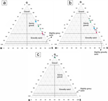
The sediments from berms, shoreface and backshore beach environments along the southern coast of the Cove were analysed. Figure 7 shows ternary diagrams with the sediment grain-size characterization following the classic Folk classification. The beach sediments consist mainly of poorly sorted sandy gravels and gravelly sands, with variable proportions of medium to coarse sand. No significant textural differences were observed among the different beach sub-environments. Backshore and shoreface environments were basically formed of gravel accompanied by medium to coarse sand (backshore) or by fine to coarse sand (shoreface; Fig. 7a,b). In the foreshore environment, at the foreshore/backshore limit, the sediments formed berm morphologies that were almost ubiquitous and usually well developed. They represent the coarsest fraction of the beach, consisting mostly of gravel (Fig. 7c), occasionally of gravel with very scarce coarse sand (P4; Fig. 7c) or with scarce shell fragments. Gravels were usually made of prolate and well-rounded volcanic and metamorphic clasts. Sand dominated in P2 and P1, especially in backshore environments.
It was clearly shown that the southern coast of Potter Cove is predominantly undergoing coastal erosion, with ~74% of the shoreline retreating at rates of up to −2.6 m year−1. Most profiles analysed showed berm or cliff retreat accompanied by net sediment losses, confirming this erosive trend. Although localized accretion was observed, particularly near the glacier and in P4, these positive trends remain spatially limited and do not offset the overall pattern of retreat.
Waves
It is important to emphasize that the wave modelling developed in this study was not conceived to reproduce the exact timing of observed morphological changes, but rather to demonstrate the occurrence of high-energy wave events with the potential to act as erosive agents in the study area. By simulating representative severe storms, the modelling provides a process-based framework through which to understand the physical plausibility of storm waves exerting a dominant control on coastal dynamics. This approach allows us to infer the potential role of episodic high-energy events in shaping shoreline evolution, even when direct comparisons with field surveys or satellite imagery are constrained by the logistical limitations of Antarctic research.
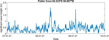
Wave observations (see earlier) were not able to capture severe wave conditions within Potter Cove. It should be noted that the ADCP was moored in a sheltered location and that visual observations were conducted only during a limited period of the summer. The mean Hs and peak period (Tp) during the monitoring period were 0.03 m and 7.3 s, respectively, while the maximum Hs recorded was 0.5 m, on 31 May 2015. In general, maximum Hs occurred during the autumn, often exceeding 0.3 m. Swell was rarely observed within the Cove; when present, it exhibited a Tp of ~20 s and Hs below 0.1 m.
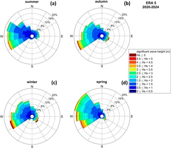
To better characterize wave conditions offshore from Potter Cove, Hs series from the ERA5 dataset (0.5° resolution) were examined at a site located at 62.5°S, 58.5°W. Five years (2020–2024) of wave data were selected for this analysis. The directional distribution of Hs exhibited no substantial seasonal differences (Fig. 8). In general, the most frequent wave direction was from the west-south-west, except in spring, when wave occurrence increased from the north-west and west-north-west. During autumn and winter, waves from the west-south-west reached higher Hs values, often exceeding 5 m. This direction is also the most favourable for severe waves to propagate into the Cove.
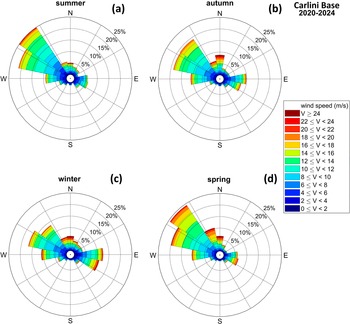
Within the Cove, wind directional distribution indicated that the most frequent winds were from the north-west, except in winter, when the occurrence of north-westerly winds decreased and winds from the west-north-west became dominant (Fig. 9). The strongest winds were generally from the north (> 24 m s−1), although their occurrence was relatively low. Winds with the longest fetches for wave generation inside the Cove were from the south-west and west-south-west, but these directions showed very low frequencies throughout the year. Therefore, if Hs (exceeding 2 m) were to occur in Potter Cove, they would probably be the result of wave systems generated outside the Cove, where the development of severe sea winds is more probable.
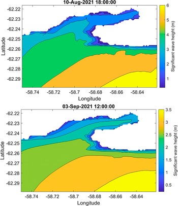
Hs outside the Cove were analysed using ERA5 data for the period 2020–2024, and two energetic events with maximum Hs exceeding 5 m were selected. Both events were simulated using the numerical model system described earlier. The modelled Hs, Tp and wave direction (Dir) at the time of maximum Hs at a point in front of Carlini Base were 2.11 m, 3.8 s and 265° (10 August 2021, 18h00 GMT) and 1.96 m, 3.3 s and 275° (3 September 2021, 12h00 GMT), respectively (Fig. 10).
The spatial distribution of Hs for both time instants mentioned in the previous paragraph is shown in Fig. 11. Maximum Hs clearly penetrated into the central part of the cove, forming a narrow tongue between the northern and southern shores that extended almost to the eastern end. It can be observed that, outside the Cove, Hs reached up to 6 m. Subsequently, transformation processes such as refraction and angular dispersion occurring during wave propagation attenuated Hs at the Cove mouth, resulting in more moderate wave conditions within the sheltered inner sector of Potter Cove.
Discussion
The combination of field data, satellite imagery and techniques from both oceanography and marine geology is essential to gaining a better understanding of coastal erosion drivers in Potter Cove. However, in the high latitudes, the availability of high-resolution optical imagery is particularly limited due to satellite orbital constraints and polar illumination conditions. Many platforms provide infrequent coverage at these latitudes, while persistent cloud cover and low sun angles further reduce the number of usable images (Fraser et al. Reference Fraser, Massom, Ohshima, Willmes, Kappes, Cartwright and Porter-Smith2020). Moreover, most automatic shoreline extraction techniques have been developed for sandy coasts and perform poorly in environments dominated by snow, ice or low spectral contrast between land and water (Yu et al. Reference Yu, Zhang, Shokr, Hui, Cheng and Chi2019). Consequently, the extensive presence of snow and ice in our study area restricts the applicability of automated approaches, requiring manual shoreline delineation with specific positional corrections. Therefore, the satellite analysis presented here is necessarily based on a limited number of available images and provides a first-order, long-term assessment of shoreline change. The integration of in situ measurements with remote sensing offered spatial and temporal insights that cannot be achieved using a single method.
Numerical models such as WW3 and SWAN were particularly useful for simulating wave parameters, and geological surveys provided information on sediment composition and shoreline changes. This interdisciplinary framework enabled a comprehensive assessment of erosion processes in this Antarctic environment and may prove useful for other Antarctic fjords. Such synergy is crucial for developing effective mitigation strategies to protect the valuable Antarctic research infrastructure.
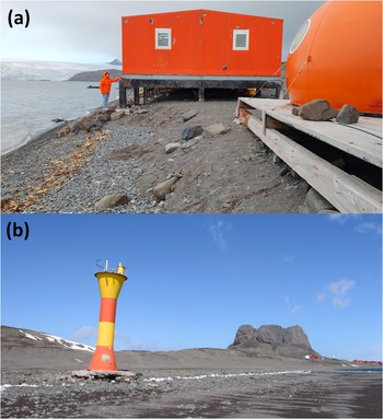
The coastal visual survey (Fig. 2a,b), the analysis of satellite imagery (Figs 3 & 5) and beach profile comparisons (Fig. 6) consistently indicated that, at least since 2020, the southern coast of Potter Cove has been experiencing progressive erosion. The situation would be less critical if Carlini Base’s piles and navigational beacon were not situated almost directly on the wrack line (Fig. 12). As a result, various alternatives to mitigate coastal erosion are currently under evaluation. However, informed decisions remain impossible to make without a comprehensive understanding of underlying causes. Sea-ice coverage and dynamics, precipitation (particularly in the form of rain) and wave and current systems are possible factors influencing coastal erosion in Potter Cove. Among these, wave impact was the main focus of this study because waves usually appear to be the main erosive agents. Nevertheless, it is difficult to determine whether waves are the most significant such factor, given that other potential drivers have not been quantitatively assessed.
Shoreline change indicators in Potter Cove: a. linear regression rate (LRR; m year−1) and b. net shoreline movement (NSM; m). Negative values (erosion) are shown in blue and positive values (accretion) in red.

Beach profiles (P) at a. P1, b. P2, c. P3, d. P4 and e. P5 measured in 2020 (blue solid line), 2023 (orange solid line) and 2025 (green solid line), referenced to mean sea level (height = 0). The Mean Higher-High Water and Mean Lower-Low Water levels are shown by red and blue dashed lines, respectively.

Folk ternary grain-size classification diagrams for selected samples, grouped by beach sub-environments: a. backshore, b. berm and c. shoreface. G = gravel; M = mud (silt + clay); S = sand.

Seasonal directional wave distributions offshore of Potter Cove (wave direction is defined as the direction from which the waves are coming), derived from ERA5 reanalysis data (2020–2024): a. summer, b. autumn, c. winter and d. spring.

Seasonal directional wind distributions within Potter Cove, based on data from Carlini Base (2020–2024): a. summer, b. autumn, c. winter and d. spring.

Simulated significant wave heights in Potter Cove during winter for two severe wave events recorded on 10 August 2021 (18h00 GMT) and 3 September 2021 (12h00 GMT).

Wave height distribution from nested numerical simulations within domain C during two intense winter events: a. 10 August 2021 (18h00 GMT) and b. 3 September 2021 (12h00 GMT).

Carlini Base: a. facility dedicated to scientific research and b. eroded foundation of the navigational beacon.

Wind waves in Potter Cove were previously simulated by Lim et al. (Reference Lim, Lettmann and Wolff2013) using the SWAN model, which remains the only numerical study on wave dynamics in the area. That study investigated wave patterns, energy fluxes and dissipation. Similarly to the present work, a nesting approach was applied, transitioning from an oceanic to a high-resolution coastal scale focused on Potter Cove. A key difference, however, lies in the simulation period: Lim et al. (Reference Lim, Lettmann and Wolff2013) modelled waves during a summer month, whereas the present study focuses on winter conditions (when wave energy may be stronger relative to the rest of the year) and particularly investigates whether severe waves can reach the inner waters of the Cove during this season. To this end, wave simulations were carried out for July, August and September 2021 - a period characterized by excellent wind data coverage. The numerical simulations indicated that waves exceeding 2 m in height could indeed occur within the Cove. Considering that both model results and limited observational data suggested significantly lower Hs during summer, the hypothesis that winter Hs are substantially greater is accepted. As a result, severe waves may propagate into the inner Cove and become the dominant erosive force during winter, especially under ice-free conditions (Fig. 11).
As shown, the highest waves propagate from the west-south-west, with Hs exceeding 5 m during autumn and winter (Fig. 8). However, winds from the west-south-west - aligned with the major axis of the Cove (west-south-west to east-north-east), which offers the largest fetch for wave generation (Fig. 1) - are infrequent within the Cove (Fig. 9), suggesting that the most energetic wave events originate offshore. These waves are particularly erosive during ice-free conditions. It is improbable that severe waves (Hs ≈ 2 m) can be generated locally due to the spatial limitations of Potter Cove (~4 km long). Under fetch-limited conditions, such as those occurring inside the Cove, the wind must blow consistently over a sufficient distance and duration for Hs to reach equilibrium at the end of the fetch. Hasselmann et al. (Reference Hasselmann, Ross, Muller and Sell1976) developed a parametric model describing wave growth under these circumstances. Assuming a maximum local fetch of 3 km from the west at the simulated location (SWAN point; Fig. 1), a constant wind speed of 35 m s−1 would be required to produce Hs of 1.6 m. Notably, the highest wind speed ever recorded at Carlini Base was indeed 35 m s−1, originating from the north-east. Moreover, such wind speeds were not observed during the winter of 2021. Therefore, the wave simulation with Hs values exceeding 2 m strongly supports the conclusion that the most energetic waves originated offshore, in the adjacent Maxwell Bay or Bransfield Strait (Fig. 1). On the other hand, eight wave events with Hs ≈ 1 m were obtained during the simulated winter (Fig. 10). They could be generated both inside and outside the Cove. Although their abrasive effect is moderate, they are energetic enough to erode the beach. It has been demonstrated that the cumulative impact of a series of moderate wave events can be more erosive than that of a single, more severe event (Ferreira Reference Ferreira2005).
The ability of high-energy waves to propagate into the inner Cove under ice-covered conditions depends on several factors, including the fractional ice coverage, its spatial distribution across the outer and inner Cove and the physical properties of the ice (e.g. thickness, concentration and mobility). In general terms, when a substantial portion of the Cove is covered by sea ice, the ice acts as an effective mechanical buffer, attenuating wave energy through scattering, dissipation and flexural damping processes.
Under such conditions, it is expected that incoming wave energy would experience significant attenuation before reaching the inner Cove, making the preservation of offshore Hs within the inner basin improbable. A considerable fraction of the wave energy would be absorbed or dissipated by the ice cover, thereby limiting the direct impact of high-energy waves on the inner coastal sectors. Consequently, the influence of wave-driven erosion during ice-covered periods is expected to be strongly reduced compared to under ice-free conditions.
However, due to the lack of detailed, high-resolution observations of ice concentration and distribution during winter conditions in the study area, a quantitative assessment of wave penetration under ice-covered scenarios remains beyond the scope of this study and represents an important limitation to be addressed in future work.
The potential for sand in the surf zone near Carlini Base to be mobilized by winter waves was also assessed. In this area, beach sediments consisted of poorly sorted sandy gravels and gravelly sands, with varying proportions of medium to coarse sand. By combining the expression for the initiation of sand motion under oscillatory flow conditions proposed by Hallermeier (Reference Hallermeier1980) with the equation for maximum horizontal orbital velocity at the seabed derived from linear wave theory (Dean & Dalrymple Reference Dean and Dalrymple1991), it was determined that sand with a median diameter (d 50) of up to 2.0 mm, in coastal waters 1 m deep, will be set into motion if Hs exceeds 0.30 m. Considering that Hs inside Potter Cove can easily reach 1 m during winter (Fig. 10), it is concluded that waves act as effective erosive agents along the south-east of Potter Cove’s coastline. In addition, the Dean number (Dean & Dalrymple Reference Dean and Dalrymple2004) calculated for sediment with a d 50 of 0.002 m indicates that, for Hs exceeding 1.2 m and periods of ~3 s, the beach profile falls within the destructive regime (i.e. one dominated by erosional processes). Therefore, events similar to those described earlier (Fig. 11) are likely to have contributed to erosion along the southern coast of Potter Cove. In addition, winter waves can induce wave set-up, defined as the positive change in mean water level caused by the presence of wave trains (Bowen et al. Reference Bowen, Inman and Simmons1968). When combined with a storm surge, this effect can significantly elevate sea levels, allowing waves to reach normally dry areas and eventually erode the foundations of the facility dedicated to scientific research at Carlini Base (Fig. 12a).
Coastline morphology is a primary factor controlling the dynamics of erosion, transport and accumulation of littoral sediments, with deposition typically prevailing in bays and erosion at headlands. However, the observed geomorphological features suggest that additional factors influence the overall sediment accumulation-erosion pattern in the study area. Firstly, the presence of hooked spits indicates that longshore drift plays a significant role in sediment transport and deposition within Potter Cove, especially to the east of Carlini Base, where modern hooked spits are found. Secondly, the occurrence of deltas and alluvial fans in the inner sector of the Cove - fed by ephemeral fluvial systems linked to retreating glaciers - indicates a substantial glaciofluvial sediment supply to the inner sector of the Cove, especially associated with Carlini and Oscar creeks (Fig. 1). Thirdly, the presence of marine terraces provides evidence of coastal progradation associated with isostatic rebound following glacial retreat. Examples of this process are the marine accumulation terraces that form Elephant Point (Heredia Barion et al. Reference Heredia Barión, Lindhorst, Schutter, Falk and Kuhn2019).
The textural characteristics of the sediments confirm a predominantly glacial and glaciofluvial origin, with subsequent reworking by wave action and longshore currents along the coast, as shown by the scarcity of finer fractions of sediments in the backshore, shoreface and berm environments. The low percentage of fine sediment fractions in the analysed samples suggests that fine sediment washing is a dominant process, most probably due to wave action (Fig. 7). Conversely, the relative abundance of fine sediments at the backshore and shoreface of P1 is attributed to its proximity to glacier runoffs from Fourcade Glacier that deliver clayey silts and finer sands to the shore. The presence of incipient cliffs in moraine deposits and palaeo-cliffs on marine terraces reveals that erosion remains a significant process, even in zones primarily dominated by accumulation, and this has intensified in recent times. This increase could be linked to variations in wave dynamics or in the frequency and intensity of storm events, which can trigger phases of accelerated erosion in recent times. Supporting this interpretation is the presence of gravel beach ridges (Fig. 6), commonly regarded as deposits formed by high-energy storm waves (Heredia Barión et al. Reference Heredia Barión, Lindhorst, Schutter, Falk and Kuhn2019). Finally, the potential effects of reduced glacial sediment input should not be overlooked, as the highest sediment fluxes typically occur during the initial stages of glacier retreat. A decline in sediment supply could alter the erosion-accretion balance within the Cove, potentially enhancing the erosive impact of wave action.
Conclusion
This study highlights the importance of severe wave events as potential erosive agents along Antarctic coasts. The wave modelling was specifically designed to demonstrate the occurrence of high-energy storms and their physical plausibility as dominant drivers of coastal erosion. By focusing on representative severe events, the results emphasize the role of storm-induced hydrodynamics as a key mechanism shaping shoreline evolution under polar conditions. Although the temporal mismatch between modelled storms and available observations prevents a direct cause-effect validation, the occurrence of severe Hs strongly supports the interpretation that storm activity is one of the main forcing factors behind the erosion documented in profiles such as P1 and P5. This indirect but consistent line of evidence is particularly relevant in Antarctica, where continuous monitoring is logistically infeasible and episodic high-energy events may leave long-lasting geomorphological imprints only detectable months or even years later.
Historically, visual observations and limited measurements obtained during summer campaigns suggested that wave energy within the Cove was low and insufficient to cause significant erosion. However, this study numerically simulated wave conditions during the winter months (July, August and September 2021) and revealed two severe wave events with Hs ≈ 2 m and eight additional events with Hs ≈ 1 m occurring inside Potter Cove (Figs 10 & 11). The most energetic events (Hs ≈ 2 m) were generated offshore - in Maxwell Bay or the Bransfield Strait - and propagated from the west-south-west directly through the mouth of the cove. In contrast, the more frequent, moderate events (Hs ≈ 1 m) could originate either inside or outside the Cove. The current sea-ice coverage reduction in the West Antarctic Peninsula is diminishing the natural wave-buffering effect and thereby enhancing the erosive impact of wave activity on the shoreline.
A key limitation of this study is the lack of quantitative high-resolution observations of sea-ice concentration and distribution during winter. Although sea ice is expected to strongly attenuate incoming wave energy and reduce wave-driven erosion within the inner Cove, the absence of quantitative ice data prevents the direct assessment of wave penetration under ice-covered conditions, which should be addressed in future work.
Although wave action appears to be the primary agent driving coastal erosion in the southern sector of Potter Cove, its relative importance remains uncertain. The lack of quantitative assessments of other potentially relevant processes (e.g. permafrost thawing, glacier meltwater discharge, sea-level variability or changes in sediment supply) limits our ability to fully characterize the erosional dynamics affecting the area. Therefore, a comprehensive understanding of the contributing factors requires future multidisciplinary studies that integrate physical, oceanographic and geomorphological data. The coastal erosion observed during the relatively short periods of the present study and the ongoing anthropogenic climate change pressure over the West Antarctic Peninsula highlight the urgency of developing multidisciplinary coastal erosion risk assessments for the valuable Antarctic research infrastructure.
Declaration of AI-assisted technologies in the writing process
This manuscript was entirely written by the authors. ChatGPT (OpenAI, 2024) was used to enhance language and readability, including grammar, spelling, punctuation and overall clarity and fluency. After using this tool, the authors thoroughly reviewed and edited the content as needed and take full responsibility for the final version of the manuscript.
Author contributions
Conceptualization (AS, ERB, GT, GB, WD), data curation (AS, CB, SV, MS, JMA, MF), formal analysis (AS, ERB, CB, GB, WD), funding acquisition (GT, EI, VF), investigation (AS, ERB, WD), methodology (AS, CB, SV, GB, WD), project administration and resources (GT, EI), software (AS, CB, SV), supervision (WD), validation (AS, SV, JMA, MF), visualization (AS, SV, CB, MS, JMA. MF), writing - original draft (AS, ERB, CB, GB, WD), writing - review and editing (MS, GT, GB, EI, WD).
Acknowledgements
We thank the UE IMCONet project (FP7 IRSES, 319718), a cooperation between the Instituto Antártico Argentino/Dirección Nacional del Antártico and the Alfred Wegener Institute - especially the late Doris Abdele - for their support. We also acknowledge the Total Foundation through the Eclipse Project, in particular Cova Oreja Saco del Valle, Alejandro Olariaga, Juancho Movilla, Marcos Tatián, Ricardo Sahade and Gastón Alurralde, for facilitating some of the field data. Special thanks are given to Andrés Pescio, Fernando Becker, Lucía Chesta and Luciano Banegas for conducting beach profile surveys, and to the Carlini Base staff during the summer campaigns of 2020, 2023 and 2025.
Financial support
This work was supported by the Instituto Antártico Argentino/Dirección Nacional del Antártico and the Servicio de Hidrografía Naval de Argentina/Ministerio de Defensa de Argentina.
Competing interests
The authors declare none.

 Open access