


1. INTRODUCTION
The purpose of this paper is to present the first dedicated investigation into the existence, life cycle and geographical spread of ice sails. Ice sails are an intriguing feature of some debris-covered glaciers, albeit one that is rare and esoteric (see Figs 1, 2). In explaining what an ice sail is, and how one evolves and decays, we hope to demonstrate that they are a distinct species of glacier surface phenomenon, separate, say, from penitentes (as suggested by Workman and Workman (Reference Workman and Workman1917)) or collapsed seracs (as suggested by Jacot-Guillarmod (Reference Jacot-Guillarmod1904)). Our analysis suggests the following as a suitable definition of an ice sail: An isolated clean ice melt feature, typically with clearly defined ridges and broadly flat faces, that protrudes from a debris-covered glacier for several years.
A collection of ice sails on the Baltoro Glacier, Karakoram range, Pakistan. The ice sails are ~10–12 m high, the camera is facing SSE, and Masherbrum is the prominent mountain seen in the upstream distance. Photo: A. Lambrecht, 2011.

A series of ice sails on the Urdok Glacier, Karakoram range, Pakistan. For scale, the second author can be seen standing next to the base of the leftmost ice sail, adjacent to some meltwater. The camera is facing SE. Photo: A. Lambrecht, 2006.

In the past, ice sails had been referred to as ice pyramids or ice pinnacles, but more recently the name ‘ice sail’ was suggested in a paper by Mayer and others (Reference Mayer, Lambrecht, Belo, Smiraglia and Diolaiuti2006), in which an analysis of the debris cover of Baltoro Glacier in the central Karakoram region of Pakistan was presented. They were so named for, as one views these structures in the distance, their relatively flat-sided faces with clearly defined ridges and often high reliefs (see Fig. 2 for a specimen over 25 m tall) give the appearance of the sails of a boat cruising over the debris-covered surface – a comparison also made nearly 100 years earlier by de Filippi (Reference de Filippi1912). Despite the striking appearance of ice sails, only a handful of published references to these structures have been made, mainly (except for Mayer and others (Reference Mayer, Lambrecht, Belo, Smiraglia and Diolaiuti2006)) from before the mid-20th century and are generally in regards to the Baltoro Glacier.
The first documented reference to ice sails that we are aware of was by Godwin-Austen (Reference Godwin-Austen1864), who, on the Baltoro Glacier, observed them to be ‘huge masses of ice in detached blocks, some long and ridged, others pointed, but all in a perfectly continuous line, and which gave the idea that they had been forced up’. Further illuminating references to the Baltoro ice sails include those given by: Jacot-Guillarmod (Reference Jacot-Guillarmod1904) who suggested they are remnants of fallen seracs; Ferber (Reference Ferber1907) who was ‘struck by the extraordinary appearance of some ice-pyramids, which stood out in striking contrast with the moraine, and the origin of which we tried in vain to discover’; de Filippi (Reference de Filippi1912), who during an exploration of the Karakoram observed ice sails lying ‘in rows running in the direction of the moraine’; Workman and Workman (Reference Workman and Workman1917), who suggested ice sails were ‘a gigantic form of ice-penitente’, created as upthrust structures caused by the crowding together of multiple upstream glacier catchment basins, which are then subject to melting, eventually leaving them ‘standing detached from one another as the ice-pinnacles in question’; Visser (Reference Visser1932), whose photographs of them were published in his account of his 1929/30 exploration of the Karakorams; and by Fisher (Reference Fisher1950), who sought to compare ice sails to the termination of wave structures on Swiss glaciers – a publication, which included an image of a 45 m high ice sail!
References to ice sails outside the Karakoram come from the Mount Everest region: Bruce (Reference Bruce1923) and Norton (Reference Norton1924). These publications noted and photographed ice sails on the Rongbuk Glacier as part of expedition reports by British mountaineers during their 1922 and 1924 attempts on Mount Everest. In particular, Bruce (Reference Bruce1923) noted that ‘from the stony surface of the glacier fantastic pinnacles arose, a strange, gigantic company, gleaming white as they stood in some sort of order, divided by the definite lines of the moraines’; and Norton (Reference Norton1924) noted that ‘as the processes of ablation and thaw increase in the lower reaches of the glacier…[ice sails] become detached and stand in isolated masses’.
We commence our analysis with a study of ice sail photographs from the relatively well-documented debris-covered glaciers of the Karakoram mountain region. We then conduct a satellite image analysis in which we examine the evolution of ice sails over a 13-year period, as well as their geographical occurence. To supplement the sparse observations of ice sails, we create an energy-balance model that is consistent with our primary data and satellite information. We are able to predict the mass-balance sensitivities of ice sails towards changes in various energy fluxes, as well as explaining their rarity.
2. ICE SAIL CHARACTERISTICS
We have primary field observations of ice sails from five field trips to the central Karakoram mountain region: the Baltoro Glacier in 2004, 2011 and 2013 (Mayer and others, Reference Mayer, Lambrecht, Belo, Smiraglia and Diolaiuti2006; Mihalcea and others, Reference Mihalcea2006, Reference Mihalcea2008; Collier and others, Reference Collier2013); the Urduk Glacier in 2006 (Mayer and others, Reference Mayer2014); and the Hinarche Glacier in 2008 (Mayer and others, Reference Mayer2010), see Figure 3 for location. These glaciers are all tens of kilometres long (the longest, Baltoro Glacier, is 62 km long), and exist in relatively dry conditions during the ablation period. The elevations at which these glaciers ice sails reside are ~4250 m (Baltoro), 4600 m (Urdok) and 2850 m (Hinarche) (we note that the lowest, Hinarche Glacier, has the fewest and smallest ice sails). All three glaciers have significant debris coverings, and debris encircles every ice sail. Debris cover on glaciers typically increases in coverage and thickness down glacier at a rate that is dependent on the relative importance of melt-out of debris from the glacier and advection of surface debris towards the terminus by ice flow (e.g. Kirkbride, Reference Kirkbride2000) – the termini of these three glaciers all support a continuous cover of rock debris. The average debris thickness where the Baltoro Glacier ice sails have been observed ranges from ~4 cm where they first regularly appear, to ~13 cm some 7.5 km further downstream (Groos, Reference Groos2016), where they cease to exist (the debris cover being a mix of dust and clasts typically of a few cm to 20 cm diameter, with some isolated larger boulders). Such depths are comparable to elsewhere in the Karakoram region, which has an average debris thickness of ~23 cm (Minora and others, Reference Minora2015). With the Baltoro Glacier flowing at ~100 m a−1 (Mihalcea and others, Reference Mihalcea2006), one can infer the debris layer thickens on average by some 1.2 mm a−1, although there will be much local variabilty.
A map of the Karakoram mountain range, showing the location of nine glaciers, which clearly have ice sails (orange) and the remaining glaciers which do not appear to have them (blue).

The Karakoram field trips all found that in the broad vicinity of the ice sails the surrounding debris-covered ice was melting (see Fig. 2, which shows melt water at the base of an ice sail), a point that was also noted for Baltoro Glacier a century earlier (Workman and Workman, Reference Workman and Workman1917). In the Baltoro Glacier case, the melt rate was typically of the order of 4 m a−1 (Mihalcea and others, Reference Mihalcea2006). Combining this fact with the knowledge that individual ice sails can persist for multiple decades (see analysis below) without growing to heights of hundreds of metres, implies that their ablation rates must be comparable with those of their surrounding debris-covered portions of the glacier. Consequently, the dominant ablation process for the Karakoram ice sails must be melting, because the alternative, sublimation, is a far slower mass removal process and thus the ice sails would reach much greater heights than those observed.
The examined ice sail images show some common characteristics. The first is the existence of clearly defined steep ridges at the top of the ice sails, where the distinct sloping sides of the ice sail meet (Figs 1, 2, 4–6). Many ice sails have multiple ridges, although rarely do we see more than six upon an individual ice sail. To a first approximation, the faces of the ice sail are planar, see for example Figure 2. A crude analysis of several images showed the average angle of inclination of an ice sail face to be ~55°, with northern aspects having the steepest slopes. As one would expect, these faces can exhibit a variety of surface features, including wind scouring (here a relatively minor mass loss mechanism), historical snow accumulation layers, and a low amount of surface impurities such as rock and dust; see e.g. Figure 5.
A close-up view of two ice sails upon the Baltoro Glacier. The shorter face of the nearer ice sail has a relief of some 5 m and the camera is facing SSE. The image shows how a steep apron of clean ice has formed at the base of the north face of each of the the ice sails (facing towards the observer), and that their bases have a slightly higher elevation than that of the opposing sides. Photo: C. Mayer, 2011.

Image highlighting the Baltoro Glacier's historical snow accumulation patterns on the sides of an ice sail, that are now folded and deformed. The relief of the shorter face is ~3 m and the camera is facing SE. Photo: C. Mayer 2013.

Two images of the same Baltoro Glacier ice sail, with reliefs of ~6–7 m, and the camera is facing S. Image (a) was taken in 2011 and shows an apron of clean ice at the base of the ice sail. In contrast, image (b) was taken in 2013, and shows a thin debris layer reaching up to a similar elevation to that of the apron. The images also appear to show evidence of previous aprons higher up the face, suggesting that aprons are annual features. Photos: A. Lambrecht, 2011, 2013.

Towards the base of many of the ice sails, the gradient is observed to steepen abruptly (Figs 4, 6). This steepening produces a distinct apron around the base of the ice sail, with heights typically between 50 and 100 cm. Notably, the aprons appear most prominent on the northern faces and are least pronounced (and often non-existent) on the southern faces, suggesting that their presence is negatively correlated with the magnitude of the incoming solar radiation. Information regarding these aprons can be gained from Figure 6, which shows images of the same ice sail in 2011 (image a) and 2013 (image b); these are the only in situ before and after images of an ice sail that we have. The most recent image shows fine-grained debris elevated from the rest of the debris layer on the side of the bottom portion of ice sail, while the older image shows no sign of this debris, but does have a steep apron of clean ice – to an elevation comparable with the debris rise in the 2013 image. Both images show what appears to be the remains of former aprons higher up the ice sail. The aggregation of these observations suggests the possibility that ice sail apron formation follows a cyclical process: as the glacier melts, a thin debris layer adjacent to the ice sail ‘sticks’ to the newly formed ice surface. This helps steepen the covered ice up to the point where the debris starts to move downslope, due to the steep gradient and melting, leaving the ice apron clean and thus part of the ice sail. This process, which appears more prominent under low-incoming solar radiation, is consistent with the image of Figure 5. In the vicinity of an ice sail, the debris layer can be inclined, and debris particle size tends to be segregated from smaller to larger as one moves a few metres away from the bottom of the ice sail. These observations suggest the existence of gravity-driven debris reorganisation processes in the immediate vicinity of the ice sail, and this might play a role in maintaining the overall footprint of the ice sail at its base.
We also observed a tendency for the bottom of an ice sail's northern aspects to have a slightly higher elevation relative to the southern aspects (Figs 4, 5). This elevation difference appears to be no more than the order of a few metres, and is presumably due to the effects of the ice sail on the relative distribution of shading and reflection of incident solar radiation on the immediate surroundings of the sail. All of these geometric features (ridges, relative flatness of the ice sail sides, aprons and elevation differences) exist on the majority of the ice sail images we examined. The implication of this is that these features are independent of the ice sail's position along the glacier flow line, and thus the existence of these features needs to be compatible with all stages of the ice sail's evolution.
The fact that ice sails do not exist along the entire length of the Baltoro, Urdok and Hinarche Glaciers means that something must change sufficiently to cause their eventual demise (we note that these glaciers continue to flow at a similar gradient for several kilometres after the ice sails have disappeared). Clearly glacier elevations change as they flow downstream, but for the 10-km-long region where the ice sails are present on the Baltoro Glacier, the elevation change is only ~300 m (from ~4400 to ~4100 m) and so meteorological conditions can be expected to alter only very slightly.
A more prominent change that occurs, however, is that the debris layer significantly thickens as the glacier flows downstream: on the Baltoro Glacier the change is uniform, from ~4 cm in the region where ice sails appear to ~13 cm at the downstream point where they disappear (Mihalcea and others, Reference Mihalcea2008; Groos, Reference Groos2016). We know from considering the Østrem curve (Østrem, Reference Østrem1959) (a plot of the melt rate of debris-covered ice versus debris depth, see Fig. 7) that as the debris cover thickness increases, the melt rate transitions from being faster than that of flat clean ice to slower than the melt rate of flat clean ice. If such a transition also holds for a comparison between the majority of inclinations/orientations of planar clean ice faces and adjacent horizontal debris-covered ice, then when the surrounding debris cover has become thick enough, we expect at least one face of an ice sail to necessarily melt faster than the surrounding glacier ice, thus removing the ice sail in the process. Hence, it appears sensible to suggest that it is debris thickening that is the primary cause of the eventual ice sail demise.
The computed melt rate of a level debris-covered portion of Baltoro Glacier (solid line), versus a level clean ice equivalent using the albedo appropriate for an ice sail (dashed line), using the DADDI model of Evatt and others (Reference Evatt2016) (see Eqn (2) of the current paper). The square marks are means of measured Baltoro glacier melt rates for a given debris thickness, taken from Table 1 of (Mihalcea and others, Reference Mihalcea2006) (for measurement sites inclined by <5°). Note that the modelled bare ice ablation rate underestimates that of the field measurements as we use an albedo of 0.42 for bare ice, which is appropriate for the clean ice sails, rather than a value of 0.17, which is more appropriate for the dusted ice of the field site, and results in ablation rates in line with the field observations and gives a critical debris thickness for the transition point of ~3 cm rather than the 14 cm transition for ice sails shown in this figure.

2.1. Satellite image analysis
To analyse the evolution of ice sails, we observed the changes for 90 of the Baltoro Glacier ice sails shown in Figure 8. These Google Earth images bookend a 13-year period between the 30th June 2001 and the 26th June 2014, during which time the ice sails moved with the glacier flow by ~1350 m and the glacier melt rate was ~ 4 m a−1 (Mihalcea and others, Reference Mihalcea2006). The dates were chosen to encompass a sufficiently long-time interval to observe changes, and to sample the glacier when it was snow-free. All of the observed ice sails are in the central region of the glacier length, forming part of a 7.5-km-long sequence of ice sails. This sequence is located approximately mid-way across the glacier, on a band of debris that appears darker than all of the other debris bands. It is along the length of this sequence that the debris layer thickens from ~4 cm to ~13 cm (Groos, Reference Groos2016; Mihalcea and others, Reference Mihalcea2008). We broke the sequence of ice sails down into seven regions. These sections are shown in Figure 8b, where from upstream (right) we term these regions (number of sails in region) the: Developing Region (20), Upper Region (8), Upper-Middle Region (19), Middle Region (8), Lower-Middle Region (14), Lower Region (9) and Decaying Region (12). These seven sections are advected downstream with the flowing glacier, where the distances relative to one another remain near-constant. We note that the Developing and Decaying Regions are slightly separated from the other, closely-joined, five regions (within which the ice sails of Figs 1, 4–6 reside). In considering the changes over time for each section, we illustrate the different phases of an ice sail's evolution: ice sails are shown to grow in the Developing Region, decay in the Decaying Region, and exist relatively stably in between. Such a life cycle is consistent with the observations of de Filippi (Reference de Filippi1912), whose account reveals that the 2001/14 positions of the sequence is similar to the positions of the ice sails he observed 100 years earlier.
Satellite images of the Baltoro Glacier, taken from Google Earth. Image (a) shows the Baltoro Glacier, with the red inserts indicating the locations of images (b) and (c) – the location of (a) is shown in Figure 3. The locations of the seven regions of the analysed ice sail sequence are shown in image (b). Image (c) shows the ice sails that appear to ‘float off’ downglacier from the termination of the medial moraine/clean ice bands (although in reality they are fixed upon the glacier surface).

2.1.1. Ice sail development
There appear to be at least two mechanisms through which ice sails can form. The first mechanism can be seen by noting the ice sail sequence of Figure 8 is separated from all other glacier surface areas containing clean ice upstream by several kilometres of debris-covered ice. This suggests that the ice sails are created locally by some sort of ‘instability’ (Fowler and Mayer, Reference Fowler and Mayer2017) as they are advected downstream. This local instigation is also suggested by studying images of the Developing Region, Figure 8b, over the 13-year window. Here we observe that the fully developed ice sails of 2014 appear to correspond to the areas of patchy debris cover from 2001 (Fig. 9). This confirms that there is a debris reorganisation process going on in the Developing Region, whereby the patchy ice becomes increasingly clean. In a similar manner to the ice sail apron formation, this debris reorganisation is presumably helped by a combination of differential melt rates associated with the Østrem curve (see Fig. 7) and ice sail steepening, which would allow debris to move downslope thereby leaving the upper slopes clean.
Satellite images taken from the Developing Region of the Baltoro Glacier ice sail sequence. Image (a) is from 2001, and image (b) is from 2014.

The second mechanism that appears to be able to produce ice sails can be observed by looking 3 km further upstream of the Developing Region, to the region where the glacier surface has distinct longitudinal bands of medial moraines and clean ice (Fig. 8c). As the bands move downstream, the undulating surface of the clean ice portions gradually allows debris to fall laterally from the moraines into the low points of the clean ice bands. This process eventually leads to the clean ice bands being segmented into a series of clean ice structures, each surrouded by newly debris-covered ice (see Anderson (Reference Anderson2000); Kirkbride and Deline (Reference Kirkbride and Deline2013) for further discussion of debris reorganisation). Visually, this has the effect of large sections (tens of meters in width) of ice ‘floating’ off from the front end of the clean ice bands (Fig. 8c). At this final stage, the satellite images of these isolated clean-ice pinnacles show them as having distinct ridges, meaning that by this point they too can be considered ice sails. This same ice sail creation mechanism for Baltoro was also suggested by de Filippi (Reference de Filippi1912) and is consistent with the explanation given by Norton (Reference Norton1924) in regard to Himalayan ice sails.
2.1.2. Ice sail persistence
To provide qualitative insight into the evolution of fully formed ice sails, Figure 10 shows the change between the eight ice sails of the Middle region, over the 13 year period. It can be seen clearly that the ice sails have changed size and shape only very slightly over this time period. For example, the main ridge on ice sail 1 has moved a few metres eastwards, whereas the main ridge on ice sail 8 has moved westwards (the changes being relative to the centre of the ice sail footprint); ice sail 8 has gained footprint area, whereas ice sail 1 has lost footprint area. From observing ridge changes in all seven of the regions, we observed no overall directional bias. We also saw no strong differences between ridge orientations for each region. These results suggest that, once formed, ice sail orientations are reasonably stable.
Satellite images taken from the Middle Region of the Batoro Glacier ice sail sequence. Image (a) is from 2001, and image (b) is from 2014. The numbers identify the corresponding ice sails.

The total ice sail basal surface area of each region declines with downstream distance and hence with time (Fig. 11; we do not plot the results for the Developing Region, as the majority of the sails are not clearly defined in the 2001 image – implying that they can form in under 13 years). The Upper Region has a slight growth in ice sail basal surface area, but after that point the net change in basal surface area is increasingly negative as one looks downstream towards the point where ice sails disappear. These results suggest that as the ice sails move downstream they are more prone to decay and that this propensity increases as the ice sails age.
(a) The percentage change in clean ice basal surface area, for the analysed ice sails of each region of the Baltoro ice sail sequence. (b) The percentage of individual ice sails for each region of the Baltoro ice sail sequence that have lost basal surface. All changes calculated over the period of 30 June 2001 to 26 June 2014.

2.1.3. Ice sail decay
Ice sails can disappear very rapidly; in the 2014 satellite image we see no sign of at least five of the ice sails that were present in the 2001 image (Fig. 12). This sudden change is in contrast to the apparently stable nature of all of the upstream ice sails, and happens despite there being no obvious abrupt change in debris thickness (Groos, Reference Groos2016). This observation raises the possibility that there is a certain (average) debris depth beyond which ice sails cannot stably exist. In addition to this observation, both images of Figure 12 show faint dark parallel lines on several of the ice sails. These marks are consistent with what would be deposited from wind blown dust particles or melted-out debris. Either way, the fact there is a light covering on them at all, and no similar covering on the upstream ice sail regions (apart from the Developing Region), suggests that the angle of inclination of the ice sail faces in the Decaying Region is lower than that of the upstream ice sails. In other words, we appear to see evidence of ice sail slope angles adjusting in response to a change in conditions in their immediate surroundings.
Satellite images taken from the Decaying Region of the Baltoro Glacier ice sail sequence. Image (a) is from 2001, and image (b) is from 2014.

2.1.4. Ice sail ages
The satellite images from 2001 to 2014 show that ice sails on the Baltoro Glacier persist for over 13 years. To improve upon this lower bound, we must consider the full life cycle of ice sails, and thus consider the age suggested by each of the two possible ice sail initiation mechanisms. The mean annual ice velocity is 100 m a−1 at the centre of the ice sail region (Mihalcea and others, Reference Mihalcea2006). If we assume that the ice sails of the Decaying Region within the sequence were originally formed some 7.5 km upstream at the same location as the current Developing Region, the Decaying Region ice sails can be crudely estimated to be about 75 years old. The slight separation of the middle five regions and the Developing and Decaying Regions (Fig. 8b) may reduce the confidence in this estimate, and a more conservative estimate is to use the distance between the ice sails of the Upper and Lower Regions to infer age, which suggests that the Lower ice sails are over 50 years of age. Under the alternative formation mechanism that ice sails are remnants of the longitudinal ice/debris bands, we draw out longer estimates: as the length of separation between the medial moraine/clean ice bands and the Decaying Region are over 10 km, the ice sails could be over 100 years old. Whichever mechanism is responsible for ice sail formation, it is clear that ice sails can last in excess of 50 years.
2.1.5. Ice sail distinction
Accepting the definition of an ice sail as: An isolated clean ice melt feature, typically with clearly defined ridges and broadly flat faces, that protrudes from a debris-covered glacier for several years, we can differentiate between collapsed seracs, ice sails and penitentes. While seracs which become surrounded by debris can help seed ice sails (making them direct ancestors of some ice sails), penitentes form in the absence of extensive surface debris cover. Penitentes are geometrically similar features to ice sails, which require sublimation to be the dominant form of ablation at the tips of the structures (enabled by low humidity conditions), and persistent high-angle solar radiation (Lliboitry, Reference Lliboitry1954; Cathles and others, Reference Cathles, Abbot and MacAYEAL2014; Moores and others, Reference Moores, Smith, Toigo and Guzewich2017). An initially smooth snow surface develops texture due to irregular snow metamorphism and this is exacerbated by focusing of solar radiation into these hollows with the result that more energy is supplied for sublimation in the topographic lows than the topographic highs (Bergeron and others, Reference Bergeron, Berger and Betterton2006; Cathles and others, Reference Cathles, Abbot and MacAYEAL2014; Claudin and others, Reference Claudin, Jarry, Vignoles, Plapp and Andreotti2015). Eventually, differential sublimation causes the hollow to become sufficiently deep and isolated from turbulent air flow that it develops its own microclimate, within which locally higher humidity allows melting to occur. This means that any mass loss in the hollows caused by the more energy efficient process of melting then greatly exceeds that occurring by sublimation at the penitente tips. Penitentes grow rapidly to their characteristic extreme relief form, with their alignment and inclination dictated by the solar arc across the sky. Penitentes are therefore related to ice sails by being caused by differential ablation. However, penitentes form in groups as the result of an instability governed by the interaction of radiation with snow topography, whereas ice sails are isolated features governed primarily by the local distribution of surface debris.
3. GEOGRAPHICAL SPREAD
To the best of our knowledge (gained through Google Earth satellite image searches and the literature), ice sails exist predominantly in the Karakoram mountain range. We were able to locate six additional glaciers within the Karakoram region that support ice sails (all highlighted in Fig. 3): Khurdopin Glacier (36 17 16 N 75 28 25 E), Sumaiyar Bar Glacier (36 09 08 N 74 52 17 E), Crown Glacier (36 06 10 N 76 09 08 E), North Crown Glacier (36 11 02 N 76 12 13 E), Yukshin-Garden Glacier (36 19 42 N 75 27 05 E) and Skamri Glacier (36 3 12 N 76 13 43 E). We found that both of the proposed ice sail creation mechanisms appear commonplace. It appears that the Khurdopin and Crown Glaciers have ice sails originating through debris reorganisation, and the Urdok, Hinarche, Yukshin-Garden and Sumaiyar Bar Glaciers have ice sails detaching off the front of the medial moarine/clean ice bands. Both ice sail creation mechanisms appear to be occurring on the North Crown, Skamri and Baltoro Glaciers.
The only other areas we could find ice sails were on some of the high Himalayan glaciers. Clear examples of Himalayan ice sails can be seen on: the East Rongbuk Glacier (Tibet, see Fig. 13) and Khumbu Glacier (Nepal), both emenating from Mount Everest; and the Kyetrak Glacier (Tibet) and Ngozumpa Glacier (Nepal), both emanating from Cho Oyu (note that the Ngozumpa Glacier ice sails are not visible in images after 2012, and so we cannot rule out the possibility that they were only temporary features). In all four of these Himalayan examples, the ice sails that are clearly visible from a satellite image analysis all appear to originate in longitudinal ice/debris bands. In addition, supraglacial streams in the immediate vicinity of the ice sails can clearly be seen (e.g. Fig. 13), showing that melting is an active process at the ice sail locations.
A snow-free satellite image of the Rongbuk glacier (28 03 50 N 52 31 00 E), where ice sails are visible in the darker right half of the image. The visible meltwater channel shows that melt as a key mass balance process. From looking at the ice sail shadows and knowing the image date and time, these ice sails have been estimated to be ~24 m in height. The lower left of the image shows part of a longitudinal ice/debris band, where the glacier is flowing diagonally up and to the left.

There are many other regions throughout the world that have glaciers with significant debris covers but do not have any documented ice sails: the European Alps, Patagonia, the Andes, Alaska, New Zealand, etc. The key to explaining this disparity appears to be two factors which, combined, set the Karakoram and Himalayan glaciers apart from the rest of the world. Firstly, the glaciers of interest are all long (tens of kilometres) and gently sloped, thereby allowing ice sails and the surrounding debris layer to evolve and then persist. Such glacier lengths are not found in the Andes, the European Alps and New Zealand (except maybe Aletsch Glacier and Tasman Glacier). Secondly, the relevant glacier ablation areas in the Himalaya are relatively high, and in the Karakoram, are relatively high and dry (Maussion and others, Reference Maussion2014); for instance the July 2004 average daytime relative humidity of the debris-covered portion of Baltoro Glacier was 50% (Mihalcea and others, Reference Mihalcea2006). The reduction in bare ice melt rate at high elevations, due to reduced sensible and longwave energy fluxes, or in especially dry atmospheric conditions, due to available surface energy being consumed in latent heat exchanges, helps ice sails sustain their structure without the southern aspects melting too rapidly. Longer Patagonian and Alaskan debris-covered glacier tongues are situated at low elevations in humid conditions and experience high bare ice ablation rates. Combined, these two facets (glacier topology; low evaporation rates) suggest the Himalaya and especially the Karakoram mountain ranges are perfect, yet uncommon, glacial environments in which ice sails can exist. That said, we welcome any further sightings of ice sails that may help us improve our understanding of their prevalence.
4. ENERGY-BALANCE MODEL
Whichever initial formation processes are at play, it is evident that ice sails attain their planar faces in a matter of years, which is short when compared with their potential decadal lifetime. We now seek to explain how these planar faces persist for such timescales, whilst melting downwards at rates of ~4 m a−1, by considering the equilibrium states of an ice sail energy-balance model. Such a consideration will shed light on the root causes of the persistence of characteristic ice sail geometry, and thus the environmental constraints on ice sail existence.
To achieve this we invoke a continuity condition across the fixed point of intersection between a face and its adjacent debris layer (Fig. 14). Ignoring localised debris movements (such as the potential formation and disappearanceof aprons near the foot of the ice sail), surface continuity implies that the meltrate of the debris-covered glacier, $\dot {m}_{{\rm d}}$
, must be equal to the apparent downwardcomponent of the melt rate of the planar clean-ice surface,
$\dot {m}_{{\rm d}}$
, must be equal to the apparent downwardcomponent of the melt rate of the planar clean-ice surface, $\dot {m}_{{\rm ia}}$
, (see Fig. 14):
$\dot {m}_{{\rm ia}}$
, (see Fig. 14):
 $$\dot{m}_{{\rm d}}(H) = \dot{m}_{{\rm ia}}(\theta,H) = {\dot{m}_{{\rm i}}(\theta,H)\over \cos(\theta)}.$$
Here we have indicated explicitly that the ice normal melt rate $\dot {m}_{{\rm i}}$
depends on the surrounding average debris depth, H, (through incoming radiation from the surrounding debris layer) and the angle of face inclination, θ. As such, for each thickness H we will seek a corresponding angle for each face of the ice sail from Eqn (1). Provided all faces have positive angles of inclination, θ > 0, then a 3-D ice sail can exist stably. An automatic consequence of this model is that the ice sail will appear to stay stationary in time, despite the planar faces clearly having a horizontal component of velocity that draws the ice sail inwards – a key difference between ice sails and ice cliffs, which move relative to a glacier surface (Buri and others, Reference Buri, Pellicciotti, Steiner, Miles and Immerzeel2016). This apparent stationarity is enabled by the glacier surface lowering through melt, thus allowing the ice underlying the ice sail to eventually become part of it (Fig. 14).
$\dot {m}_{{\rm i}}$
depends on the surrounding average debris depth, H, (through incoming radiation from the surrounding debris layer) and the angle of face inclination, θ. As such, for each thickness H we will seek a corresponding angle for each face of the ice sail from Eqn (1). Provided all faces have positive angles of inclination, θ > 0, then a 3-D ice sail can exist stably. An automatic consequence of this model is that the ice sail will appear to stay stationary in time, despite the planar faces clearly having a horizontal component of velocity that draws the ice sail inwards – a key difference between ice sails and ice cliffs, which move relative to a glacier surface (Buri and others, Reference Buri, Pellicciotti, Steiner, Miles and Immerzeel2016). This apparent stationarity is enabled by the glacier surface lowering through melt, thus allowing the ice underlying the ice sail to eventually become part of it (Fig. 14).
A schematic diagram of our ice sail model. Here we consider one face of the ice sail at a time, complete with the debris layer intersection (we neglect any localised debris movements). The ice sail is inclined at an angle θ to the horizontal and maintains its angle for a given debris depth, and its footprint. The normal melt rates of the debris layer and ice are given by $\dot {m}_{{\rm d}}$
and
$\dot {m}_{{\rm d}}$
and $\dot {m}_{{\rm i}}$
, respectively.
$\dot {m}_{{\rm i}}$
, respectively.
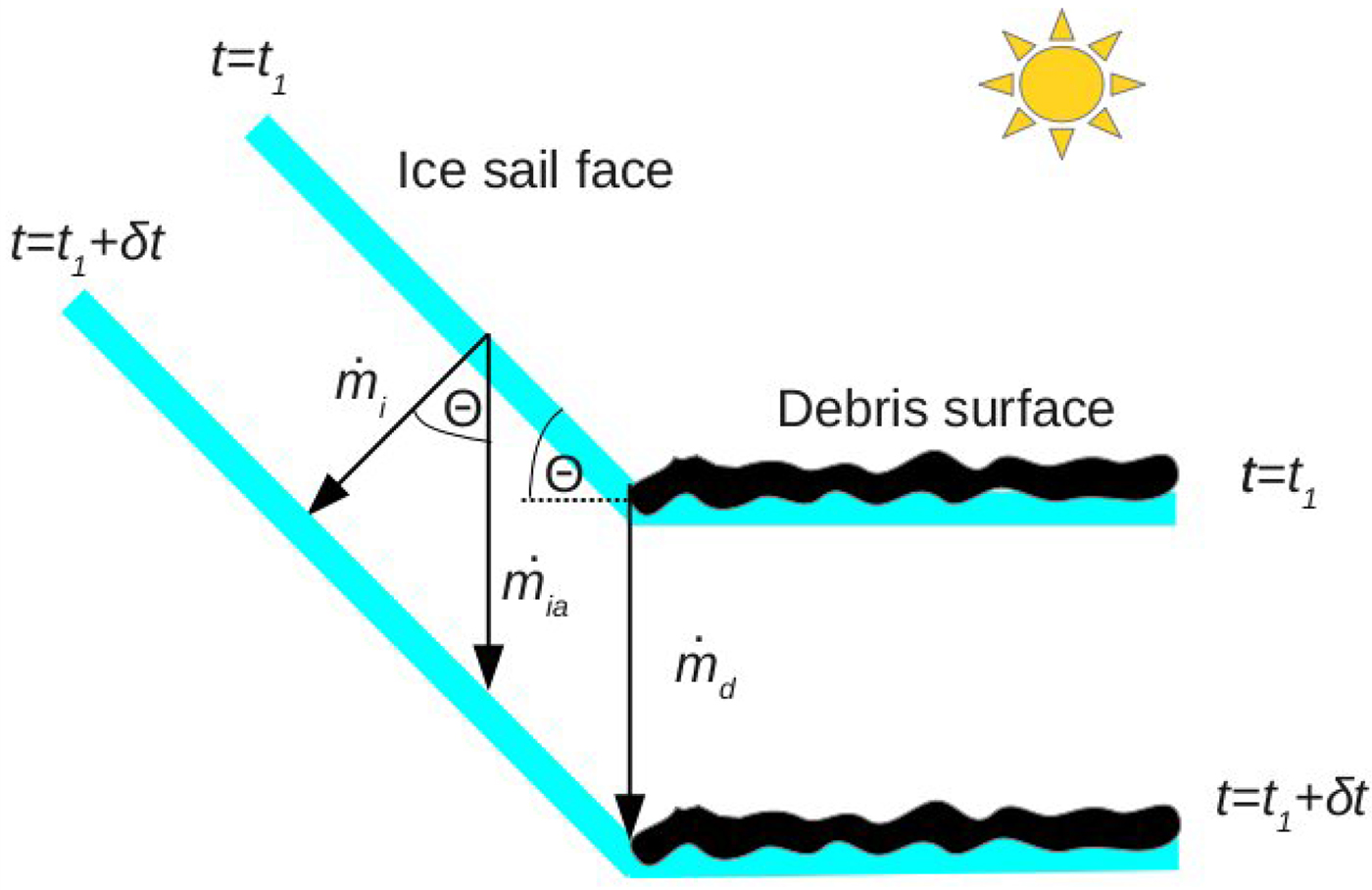
As time progresses the debris layer will gradually thicken and change the rate of melt of the debris-covered ice, so all the corresponding face angles must adjust to maintain continuity necessitated by (1). We do not explicitly consider the time-evolution of the ice sails for this initial study, as the rate of adjustment of the sail face angles is very slow as compared with the rate of loss of mass removed from the ice sail, i.e. the ratio of debris thickening rate (mm per year) to ice sail absolute loss (metres per year) is very small and hence a steady-state assumption is valid. Thus, the face angles have plenty of time to adjust to the new depth of debris. Yet, if the debris layer thickens to a point where a positive value of θ can no longer exist for any one face, then the ice sail cannot persist, i.e. if the apparent rate of melt of ice is faster than the melt rate of debris-covered ice, the ice sail will decline back into the debris layer. Around this point, continuity implies that the debris would encroach (initially by aeolian processes) onto the flattening/declining faces (e.g. Fig. 12), thereby removing the bare ice feature. We term such a critical debris thickness the extinction thickness. We aim to show that its value increases with increasing high and/or dry conditions, and that results of computations parametrised for Baltoro Glacier compare well the observed mean extinction thickness (i.e. ~13 cm).
To prescribe equations for the melt rates of debris-covered ice, $\dot {m}_{{\rm d}}$
, and clean ice,
$\dot {m}_{{\rm d}}$
, and clean ice, $\dot {m}_{{\rm i}}$
, we use those that were presented in Evatt and others (Reference Evatt2015), which successfully reproduce the non-monotonic shape of the Østrem curve. The model presented in that paper considered the balance between the energy fluxes of solar radiation, longwave radiation, sensible heat, evaporative heat, melting and heat conduction into the debris layer. Simplifying assumptions within the model are: temperate ice, long-enough timescales (hours) for a quasi-steady version of the heat equation to be used, and a linearisation of the outgoing longwave energy function. The results given in Evatt and others (Reference Evatt2015) gave close agreement with measured data of Nicholson and Benn (Reference Nicholson and Benn2006), and a mathematically similar model performed well against laboratory measurements in Evatt and others (Reference Evatt2016), and we thus continue to make use of these same assumptions here. In so doing we can simply state the equation for the normal component of the melt rates of bare ice and debris-covered ice as, respectively:
$\dot {m}_{{\rm i}}$
, we use those that were presented in Evatt and others (Reference Evatt2015), which successfully reproduce the non-monotonic shape of the Østrem curve. The model presented in that paper considered the balance between the energy fluxes of solar radiation, longwave radiation, sensible heat, evaporative heat, melting and heat conduction into the debris layer. Simplifying assumptions within the model are: temperate ice, long-enough timescales (hours) for a quasi-steady version of the heat equation to be used, and a linearisation of the outgoing longwave energy function. The results given in Evatt and others (Reference Evatt2015) gave close agreement with measured data of Nicholson and Benn (Reference Nicholson and Benn2006), and a mathematically similar model performed well against laboratory measurements in Evatt and others (Reference Evatt2016), and we thus continue to make use of these same assumptions here. In so doing we can simply state the equation for the normal component of the melt rates of bare ice and debris-covered ice as, respectively:
 $$\dot m_{\rm i} = \nu _1^i - \displaystyle{{\mu _1} \over {\mu _2 + 1}}{\rm ,}$$
 $$ \dot{m}_{{\rm d}} = {\nu_1\over 1+ \nu_2 H} - { \mu_1\over \mu_2+ e^{\gamma H}}, $$
in which the constants are defined as
 $$\nu _1^i = \displaystyle{{I_{\rm i} - {\rm \epsilon }_{\rm i}\sigma {\bar T}^4 + Q_{\rm i}(1 - \alpha _{\rm i}{\rm )} + \beta T_{\rm m}} \over {{\rm (}1 - \phi {\rm )}\rho _{\rm i}L_{\rm m}}},$$
 $$\mu _1 = \displaystyle{{L_{\rm v}u_*^2 {\rm (}q_{{\rm sat}} - q{\rm )}e^{ - \gamma x_{\rm r}}} \over {(1 - \phi {\rm )}\rho _{\rm i}L_{\rm m}u_{\rm r}}} ,$$
 $$\mu _2 = \displaystyle{{{\rm (}u_{\rm m} - 2u_{\rm r}{\rm )}e^{ - \gamma x_{\rm r}}} \over {u_{\rm r}}},$$
 $$\nu _1 = \displaystyle{{I_{{\rm at}} - {\rm \epsilon }_{\rm d}\sigma {\bar T}^4 + Q_ \downarrow {\rm (}1 - \alpha _{\rm d}{\rm )} + \beta T_{\rm m}} \over {{\rm (}1 - \phi {\rm )}\rho _{\rm i}L_{\rm m}}},$$
 $$\nu _2 = \displaystyle{{\beta + 4{\rm \epsilon }_{\rm d}\sigma {\bar T}^3} \over k}{\rm ,}$$
 $$\beta = \displaystyle{{\rho _{\rm a}c_{\rm a}u_*^2 } \over {u_{\rm m} - u_{\rm r}{\rm (}2 - e^{\gamma x_{\rm r}}{\rm )}}},$$
where the parameters are defined in Table 1. We note that the shortwave radiation, Q i, and longwave radiation, I i, felt by the ice sail both depend on the angle of inclination θ; we shall shortly determine their functional forms.
Parameter values representative of July daytime conditions on the Baltoro Glacier. See text for the parameter value provenance
We will restrict our model to consider only average day time energy fluxes during the ablation season, as this is when most melting occurs. We make this approximation for the sake of elucidation, simplicity and an absence of more detailed field measurements. We neglect the lag effects of the cold-sink that could build up within the ice sail and debris layer over night, as this consideration is unlikely to affect the equilibrium solutions we seek here. As we shall see, our computed melt rates turn out to be in good agreement with the observed melt rates of Baltoro Glacier, and thus our modelling assumptions appear reasonable. It is of note that close analogies to the energy-balance aspect of our model may be found in the study of ice cliffs, e.g. Han and others (Reference Han, Wang, Wei and Liu2010); Reid and Brock (Reference Reid and Brock2014); Buri and others (Reference Buri, Pellicciotti, Steiner, Miles and Immerzeel2016).
4.1. Baltoro parameterisation
We begin our parameterisation by considering the energy-balance components that depend upon the ice sail angle of inclination, θ. The first parameter that depends upon the angle of inclination is the flux of shortwave (solar) energy that a face of an ice sail receives, Q i, which will be the sum of the direct solar radiation flux Q dir and the diffuse solar radiation flux Q diff:
 $$ Q_{{\rm i}} = Q_{{\rm dir}} + Q_{{\rm diff}}. $$
To estimate Q dir we must prescribe a path of the sun over the ice sail's face, thus capturing the gross effects of illumination and shading. To achieve this in a simple yet representative and easily replicable fashion, we model the path of the sun as that of a semicircle inclined from vertical by an angle θ l (which will vary with latitude and date), and then average the received solar flux over half a day (i.e. daylight hours). We can then estimate the average flux of direct solar radiation felt by each face of the ice sail during daylight hours by using the product between the outward facing normal of the ice sail face, n, and the direction of the incoming solar radiation, l, via the integral
 $$ Q_{{\rm dir}} = {Q_N\over \pi} \int_0^\pi \max\lpar 0\comma {\bf n} \cdot {\bf l}\rpar \ d\eta, $$
where Q N is the average normal solar flux reaching the Earth's surface (i.e. the averaged value of the solar flux that is felt by a plane on the Earth's surface that is always normal to the incoming radiation). The vectors n and l are given by
 $${\bf n} = (\sin \theta \sin \psi {\rm ,}\sin \theta \cos \psi {\rm ,}\cos \theta {\rm ) ,}$$
 $$ {\bf l} = (\cos{\eta}, -\sin{\eta} \sin{\theta_l}, \sin{\eta} \cos{\theta_l}) , $$
where η represents the hour angle of the sun and ψ is the azimuth, which is the clockwise orientation from the north of the ice sail face. The fact that we only take the positive values of the dot product ensures that we do not count the flux when the face is shaded, and the integral between 0 and π reflects the averaging over half a day.
To approximate the flux of diffuse solar radiation, Q diff, we make use of the approaches used by Han and others (Reference Han, Wang, Wei and Liu2010) and Buri and others (Reference Buri, Pellicciotti, Steiner, Miles and Immerzeel2016), which were themselves based upon empirical formulae calculated by Dozier and Frew (Reference Dozier and Frew1990); Reindl and others (Reference Reindl, Beckman and Duffie1990). The approach is to assume a fraction k d of the total downward radiation reaching the Earth's horizontal surface Q ↓ is diffuse. This means the total flux of diffuse solar radiation reaching an ice sail's face only depends upon the visible proportion of the sky, (π − θ)/π, and thus
 $$ Q_{{\rm diff}} = k_{{\rm d}} Q_{\downarrow} \left({\pi-\theta\over \pi}\right). $$
An estimate of k d is presented in Reindl and others (Reference Reindl, Beckman and Duffie1990), which states
 $$ k_{{\rm d}} = 1.4 - 1.749k_t +0.177\overline{\sin{h}}, $$
where h is angle of inclination of the sun (the overbar denotes that we use a daylight average of the downwards component). Here k t is the clearness index, given by
 $$ k_t = {Q_{\downarrow}\over Q_{{\rm sc}} \overline{\sin{h}}}, $$
where Q
sc is the solar constant (unlike Buri and others (Reference Buri, Pellicciotti, Steiner, Miles and Immerzeel2016) we have neglected the tiny (well under 1%) variations about this figure resulting from the Earth's eccentricity). The factor that provides the average downward component of the solar fluxes for a given latitude, $\overline {\sin {h}}$
, can be calculated easily from (11) by normalising the incoming normal radiation, Q
N
= 1, and setting θ = 0, giving
$\overline {\sin {h}}$
, can be calculated easily from (11) by normalising the incoming normal radiation, Q
N
= 1, and setting θ = 0, giving $\overline {\sin {h}}=2\cos {\theta _l}/\pi $
.
$\overline {\sin {h}}=2\cos {\theta _l}/\pi $
.
In calculating the diffuse solar radiation flux via (14) and measuring the total downward solar flux Q ↓, one can calculate the normal direct solar radiation flux via
 $$ Q_{{\rm N}} = {Q_{\downarrow} - Q_{{\rm diff}}\over \overline{\sin{h}} }. $$
This means the total averaged solar flux felt on an ice sail's face, Q i, can now be written as
 $$ Q_{{\rm i}} = { Q_{\downarrow} \over \pi} \left(k_{{\rm d}}\lpar \pi-\theta\rpar + {\pi - k_{{\rm d}}\lpar \pi-\theta\rpar \over \pi \overline{\sin{h}} }\int_0^\pi \max\lpar 0, {\bf n} \cdot {\bf l}\rpar \ d\eta \right). $$
The second parameter that is a function of θ is the longwave energy flux felt by the ice sail, I i, which is received from both the atmosphere and the debris layer. To determine the flux from the debris layer we use the known result (Howell and others, Reference Howell, Menguc and Siegel2010) that if a planar surface with temperature T d degrees Celcius is joined to a second planar surface, where the interior angle is π − θ, then the longwave energy recieved by the second surface from the first, is
 $$ {\epsilon_{{\rm d}} \sigma {\lpar \bar{T}+T_{{\rm d}}\rpar ^4}\over 2}\lpar 1-\cos{\theta}\rpar , $$
where ε
d is the thermal emissivity of the debris, σ the Stefan–Boltzmann constant and $\bar {T}$
is 273 K. To prescribe the debris surface temperature we again refer to Evatt and others (Reference Evatt2015), who provided the following formula to estimate its value
$\bar {T}$
is 273 K. To prescribe the debris surface temperature we again refer to Evatt and others (Reference Evatt2015), who provided the following formula to estimate its value
 $$ T_{{\rm d}} = {\rho_iL_m\lpar 1-\phi\rpar \nu_1H\over k [1+\nu_2H] }. $$
The longwave energy flux received by the ice sail face from the atmosphere is prescribed in the same manner as the diffuse shortwave flux (14), where we simply multiply the diffuse atmospheric longwave energy flux, I at, by the visible proportion of the sky. This means the total longwave energy flux received by an ice sail face is
 $$ I_{{\rm i}} = I_{{\rm at}}\left({\pi-\theta\over \pi}\right)+ {\epsilon \sigma {\lpar \bar{T}+T_{{\rm d}}\rpar ^4}\over 2}\lpar 1-\cos{\theta}\rpar . $$
We model the solar radiation flux at the flat debris surface as simply the total downwelling radiation flux Q ↓, and the longwave radiation flux at the debris surface as that emitted by the atmosphere I at; these assumptions have already been included within the equations of (9).
The values of the remaining (θ-independent) parameters are shown in Table 1 and relate to averaged July daytime conditions of the Baltoro Glacier. The downwelling shortwave flux Q ↓, relative humidity r h and wind speed u m are all taken from automatic weather station measurements on Baltoro Glacier by Mihalcea and others (Reference Mihalcea2006). The atmospheric longwave radiation, I at, and air temperature, T m, are given by computations presented in Collier and others (Reference Collier2013) (themselves based on the measurements of Mihalcea and others (Reference Mihalcea2006)). The debris surface broadband albedo α d is set as the average of four measurements (two wet and two dry) as presented in Nicholson and Benn (Reference Nicholson and Benn2006). The broadband albedo of the clean inclined ice α i is taken as an average from Reid and Brock (Reference Reid and Brock2010) – for simplicity we neglect the fact that, as highlighted in Figure 12, an ice sail which has significantly flattened will likely have gained a higher surface dust content and thus carry a lower broadband albedo. The thermal emissivity of the ice ε i and debris ε d are taken as average values from Buri and others (Reference Buri, Pellicciotti, Steiner, Miles and Immerzeel2016). To estimate the debris layer thermal conductivity in the band where the ice sails exist (a dark shale material), we made use of a formula on p. 297 of Mihalcea and others (Reference Mihalcea2006), which when coupled with atmospheric data from Minora and others (Reference Minora2015) and temperature data from Groos (Reference Groos2016), gave values between 0.7 and 1.1 (well within the range of other reported values, e.g. Conway and Rasmussen (Reference Conway and Rasmussen2000); Nicholson and Benn (Reference Nicholson and Benn2006); Reid and Brock (Reference Reid and Brock2010)). The mid value of this range, 0.9, was used as the representative value in our modelling; a sensitivity test, presented below, explores the impact of varying this estimate. We have estimated the friction velocity u * and slip velocity u r from use of Eqn (13) of Evatt and others (Reference Evatt2015) (which makes use of the measurement height of 4 m). The surface roughness height x r and wind speed attenuation parameter γ are taken as that given in Evatt and others (Reference Evatt2015), where we note that both γ and u r have a minuscule effect on the results herein, since they only affect to the physics of debris-covered glaciers with debris thicknesses of under ~2 cm. In the absence of field measurements, we estimated the saturated absolute humidity level, q sat, from formulae stated in Vaisala (2010), namely
 $$ q_{{\rm sat}} = {1.33 \times 10^{7.59 T_{{\rm m}} / \lpar 240.7+T_{{\rm m}}\rpar } \over T_{{\rm m}}+\bar{T}}. $$
The value of the absolute humidity level then follows via q = r h q sat.
To gauge the suitability of our parametrisation, we first compute the model's predicted Østrem curve for flat debris-covered ice and the melt rate for flat clean ice, Eqn (2). We do so to compare the computed results of the debris-covered ice melt rates to the measured melt rates from different debris-covered portions of Baltoro (Mihalcea and others, Reference Mihalcea2006) for slopes of under 5°; note that each field measurement correspondents to an individual stake, which could be separated from one another by up to 100 m, meaning that each measurement likely corresponds to a distinct lithology and level of shading. The resulting Østrem curve for the debris-covered ice is presented in Figure 7. Given the inherent degree of variability in the stake measurements and our own parameter estimates, Figure 7 still shows a good agreement between the modelled and the measured data for sub-debris ablation, meaning our parametrisation appears reasonable. We do not have appropriate field data to evaluate the bare ice ablation as the field measurements of exposed ice were for dusted rather than clean ice. However, as (i) the physics/mathematics underlying our computed value for bare ice is identical to that of the well-matched debris-covered ice melt rate, and (ii) our model matches the field observations when run using an albedo appropriate for dusted ice (0.17, which is close to 0.18 for dusted ice surfaces on Miage Glacier (Brock and others, Reference Brock2010) and 0.2 recommended for debris-rich ice (Cuffey and Paterson, Reference Cuffey and Paterson2010)), we are satisfied that both the debris covered and bare ice components are simulated adequately. The critical debris thickness separating enhanced and inhibited ablation compared with that of bare ice for an ice sail is larger than those usually reported (see e.g. Reznichenko and others, Reference Reznichenko, Davies, Shulmeister and McSaveney2010) because of a combination of factors: firstly, the ice sail faces are relatively clean, and thus have a broadband albedo higher than those measured in most field studies and secondly, the relatively dry conditions of the Karakoram reduces the melt rate of clean ice (Evatt and others, Reference Evatt2015), meaning the point of intersection is pushed towards thicker debris layers.
4.2. Results
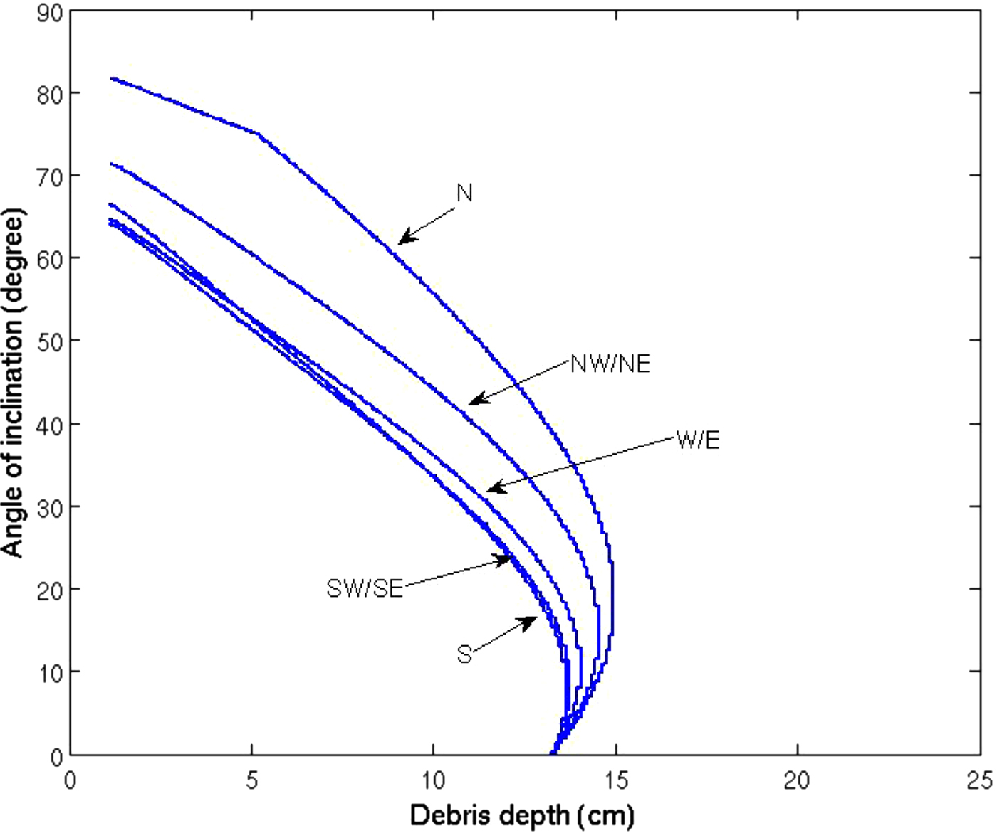
We now present solutions to our model, showing for which the range of debris layer thicknesses, H, inclined ice sail faces can exist, and their specific angles. For this purpose we consider five representative orientations of our modelled ice sail face: south, southeast/southwest, east/west, northeast/northwest and north (the nature of our model means that the energy balance during the day is symmetric about the northsouth line). Our assumption is that ice sails are faceted, with multi-planar surfaces that are orientated in any of these directions. Figure 15 shows that equilibrium angles for each face exist for debris depths below the extinction depth of ≈13 cm, in excellent agreement with the observed debris depths at which the Baltoro Glacier ice sails disappear. Beyond this debris thickness, the southern faces of the ice sail start to melt quicker than the surrounding debris-covered ice, causing the ice sail to decay (despite the other faces still having equilibrium solutions). This result also confirms the inferred decadal lifetime of the ice sails, because the average debris layer depth is a proxy for time (thickening at ~1.2 mm a−1). While in existence, the average face angle is in the region of the obseved 55°, where the slopes steepen as orientations approach north (see e.g. Figs 2, 10). The kink in the curve for the north-facing ice sail face (at 75o) is due to the inclined sun no longer being able to illuminate it. We note that the extinction depth is sometimes slightly shallower than the leading edge of the equilibrium solutions (right-most solution of a given equilibrium line). For debris thicknesses beyond any one of the leading edges, an ice sail cannot persist: here the smallest leading edge debris depth is that of the southern face, at ~13.25 cm. With this depth being extremely close to the extinction depth, we consider these two depths equivalent and refer to them under the same banner.
The computed steady-state ice sail face angles of inclination, with aspects of south, southwest/southeast, west/east, northwest/northeast, north. These are evaluated using the parameter values of Table 1.
To test the sensitivity of our results we explore the impact of atmospheric forcing parameters, showing results for the westeast case (Fig. 16). These sensitivity studies are best considered as an exploration of the geographical constraints as to where ice sails can be sustained. When the relative humidity is increased the extinction thickness reduces, meaning that a lower evaporative heat flux reduces the likelihood of ice sail persistence, which is consistent with our ice sail geographical spread analysis. In the particular example shown in Figure 16a, an average relative humidity of 38% (equivalent to a 25% increase in the outgoing evaporative heat flux) allows ice sails to persist to debris thicknesses of 15 cm, whereas an average relative humidity of 63% (equivalent to a 25% decrease in the outgoing evaporative heat flux) reduces the extinction thickness to 11.5 cm. When the average relative humidity is much higher, say at 90%, then the extinction thickness moves downwards considerably, to just 8.5 cm (not shown).
(a) the computed equilibrium ice sail face angles for faces with an east/west aspect, computed using the parameter values of Table 1, but with r h = 38%, 50%, 63% (equivalent to a ± 25% variation in the evaporative heat flux). (b) the corresponding Østrem curves for the melt rate of debris-covered ice (solid lines; all three lines overlying one another) and the melt rates of clean ice (dashed lines). The red circles highlight the points of intersection.

The melt rate of the ice sail faces, $\dot {m}_ {\rm i}$
, depends on their angle of inclination, θ, in a complicated manner. While this makes it difficult to explain why the equilibrium curves shown in Figure 16a move to the right as the humidity is reduced, we can at least explain the effect of variations in the humidity on the end-points of the equilibrium curves (i.e. for θ = 0, corresponding to a horizontal ice face). For this purpose in Figure 16b we plot the melt rates for the debris-covered ice,
$\dot {m}_ {\rm i}$
, depends on their angle of inclination, θ, in a complicated manner. While this makes it difficult to explain why the equilibrium curves shown in Figure 16a move to the right as the humidity is reduced, we can at least explain the effect of variations in the humidity on the end-points of the equilibrium curves (i.e. for θ = 0, corresponding to a horizontal ice face). For this purpose in Figure 16b we plot the melt rates for the debris-covered ice, $\dot {m}_{{\rm d}}$
, and for the clean horizontal ice surfaces,
$\dot {m}_{{\rm d}}$
, and for the clean horizontal ice surfaces, $\dot {m}_ {\rm i}$
. The results illustrate that a decrease in humidity (increase in the evaporative heat flux) causes a decrease in the melt rate for clean ice and a minuscule change in the melt rate for the debris-covered ice (this is because evaporation of the meltwater underneath a debris layer is only pronounced for very shallow debris depths (Evatt and others, Reference Evatt2015)). As a result, an increase in the evaporative heat flux shifts the equilibrium point between the melt rate curves for clean and debris-covered ice to thicker debris depths, and this trend appears to persist even for non-zero angles of inclination (Fig. 16a).
$\dot {m}_ {\rm i}$
. The results illustrate that a decrease in humidity (increase in the evaporative heat flux) causes a decrease in the melt rate for clean ice and a minuscule change in the melt rate for the debris-covered ice (this is because evaporation of the meltwater underneath a debris layer is only pronounced for very shallow debris depths (Evatt and others, Reference Evatt2015)). As a result, an increase in the evaporative heat flux shifts the equilibrium point between the melt rate curves for clean and debris-covered ice to thicker debris depths, and this trend appears to persist even for non-zero angles of inclination (Fig. 16a).
Similar behaviour can be expected if other incoming atmospheric energy fluxes (solar, longwave, sensible) are perturbed. This is because the debris layer, in effect, acts to reduce the sensitivity of the underlying ice melt rate to changes in incoming energy flux, making it less reactive to change than for a clean ice surface. Figure 17 shows the equilibrium angles of inclination against debris thickness as we vary the downwelling solar energy flux Q ↓, longwave energy flux I at, and sensible heat flux (equivalent to a variation in air density, ρ a) by ± 25%. The extinction thickness is increased/decreased by a few centimetres for a decrease/increase in incoming energy, where the largest sensitivity to the percentage change is given by the longwave energy flux. A decrease in air density, ρ a, (driven by elevation increase) thus corresponds to an increased extinction thickness, consistent with our satellite observations.
The computed equilibrium ice sail face angles with an east/west-facing aspect, where three atmospheric energy fluxes are varied by ± 25% ((a) solar, (b) longwave, (c) sensible). Other parameters as in Table 1.

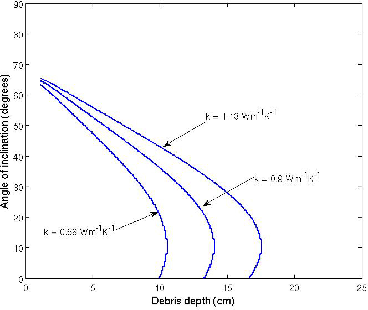
Finally, we assess the response of the model to a ± 25% change in the thermal conductivity of the debris layer, k. Figure 18 shows the resulting equilibrium angles, and indicates that an increase/decrease in thermal conductivity has the effect of increasing/decreasing the extinction thickness, because the thermal conductivity strongly influences the melt rate of the debris-covered ice.
The computed equilibrium ice sail face angles for faces with an east/west-facing aspect, where the conductive heat flux is varied by ± 25%. Other parameters as in Table 1.
5. DISCUSSION AND CONCLUSIONS
The rarity of ice sails tells us that suitable conditions for their existence are uncommon. The first requirement is for the glacier to be able to develop patches of clean ice surrounded by thin debris-covered ice, so that the more rapidly melting debris-covered ice enables mounds of clean ice to emerge from the glacier surface. From the image analysis it is evident that these clean ice features then melt to form planar faces – the characteristic ice sail shape. The second requirement is for relatively high and/or dry conditions, which decrease the sensible heat flux and increase the evaporative heat flux, respectively. These conditions serve to reduce the melt rate of the ice sail, thus allowing the structure to persist. For lower, warmer, more humid atmospheric conditions our sensitivity analysis show that inclined faces can only persist within thinner debris covers. And, as regional melt rates under such conditions are higher and meltout of debris from the glacier would result in more rapid thickening of the debris cover, in such glacier settings ice sails are unlikely to persist as they do in the Karakoram and parts of the high Himalaya. The third requirement is for the glacier to be sufficiently long, with a gentle slope, so that the ice sails are not terminated prematurely. Glacial regions which have these three requirements seem only to exist in the Karakoram and high Himalaya.
To help explain the underlying processes that govern the existence of ice sails, we developed a mathematical model for the energy balance required for an ice sail's planar faces to persist. When suitably parameterised, our model gave results in excellent agreement with ice sail observations from Baltoro Glacier, e.g. lifespan, average slope angle, existence only up to a critical debris thickness. Our model was able to show that this critical debris thickness (which we termed the extinction thickness) is defined by the depth beyond which the melt rate of debris-covered ice exceeds that of bare ice. The fact that this extinction thickness is greater in the high/dry conditions of the Karakoram than generally observed elsewhere, gives an ice sail more time in which it can grow and develop. It also allows ice sails to be resilient to the inevitable perturbations in atmospheric and debris layer conditions, as evidenced by the decadal lifetime of the Baltoro Glacier ice sails.
ACKNOWLEDGMENTS
This paper is the result of a workshop held at the International Centre of Mathematical Sciences, Edinburgh, October 2015, which was funded by the Engineering and Physical Sciences Research Council, UK, via the MAPLE Platform Grant EP/I01912X/1. IDA undertook part of this work whilst in receipt of a Royal Society Wolfson Research Merit Award and part was supported by the Isaac Newton Institute under EPSRC Grant Number EP/K032208/1. LN is supported by the Austrian Science Fund (FWF) Grant V309-N26. We thank the Department of Earth Sciences ‘Ardito Desio’, University of Milan and EvK2-CNR who provided the possibility for the field trips to the Karakoram. We are also grateful to Dr Andrew Smedley who supplied computational data for solar fluxes of Baltoro Glacier, which in the end were not used for this paper. Finally, we sincerely thank the reviewers of this paper, whose time and comments helped the finished manuscript.


 Open access