





Impact Statement
Porous trailing edges are widely used to mitigate turbulent boundary-layer fluctuations and the associated scattering of trailing-edge noise. Their performance is governed by porosity and permeability, yet these properties are typically determined only in dedicated steady-flow rigs that cannot easily reproduce unsteady hydrodynamic pressure fluctuations. We demonstrate a new method for measuring the dynamic permeability of porous materials directly under grazing-flow conditions, utilising time-resolved PIV and a lumped-system circuit analogy. This approach reveals how unsteady pressure gradients couple with through-material velocities, enabling permeability characterisation for thin trailing edges where traditional rigs are impractical. In particular, we find that internal architecture strongly governs the frequency-dependent permeability response. This work enables the study of porous add-on architectures with laser velocimetry, simplifying the design of permeable materials with targeted aerodynamic and acoustic performance.
1. Introduction
The scattering of pressure fluctuations from a turbulent boundary layer at an airfoil trailing edge in uniform, homogeneous flow is a significant contributor to broadband self-noise (Brooks et al. Reference Brooks, Pope and Marcolini1989). According to Blake (Reference Blake2012), when the trailing-edge thickness, $t$
, of an airfoil is greater than approximately four times the displacement thickness,
$t$
, of an airfoil is greater than approximately four times the displacement thickness, $\delta ^{*}$
, of the incoming turbulent boundary layers from both sides, the unsteady lift fluctuations determined by the Karman vortex shedding instability scatter in the form of a unique tonal noise contribution, in an otherwise broadband acoustic emission. The most significant tonal harmonic frequency,
$\delta ^{*}$
, of the incoming turbulent boundary layers from both sides, the unsteady lift fluctuations determined by the Karman vortex shedding instability scatter in the form of a unique tonal noise contribution, in an otherwise broadband acoustic emission. The most significant tonal harmonic frequency, $f$
, can be computed by assuming a Strouhal number of
$f$
, can be computed by assuming a Strouhal number of $St = ft/V_{\infty } \approx 0.2$
, where
$St = ft/V_{\infty } \approx 0.2$
, where $V_{\infty }$
is the free-stream velocity. Such acoustic emissions are usually referred to as blunt trailing-edge noise, and are characterised by a narrow-band component, dependent on the energy cascade of the flow-pressure fluctuations at the trailing edge. The tonal component of the acoustic spectrum is a byproduct of the scattering of pressure fluctuations due to vortex shedding associated with the roll-up process in the near wake. Therefore, efforts to mitigate this noise have focused on suppressing vortical fluctuations generated by the trailing edge.
$V_{\infty }$
is the free-stream velocity. Such acoustic emissions are usually referred to as blunt trailing-edge noise, and are characterised by a narrow-band component, dependent on the energy cascade of the flow-pressure fluctuations at the trailing edge. The tonal component of the acoustic spectrum is a byproduct of the scattering of pressure fluctuations due to vortex shedding associated with the roll-up process in the near wake. Therefore, efforts to mitigate this noise have focused on suppressing vortical fluctuations generated by the trailing edge.
1.1. Permeability and noise reduction by porous materials
The genesis and evolution of flow instabilities in the wake of bluff bodies have been widely studied for both aerodynamic and aeroacoustic purposes (Barbi et al. Reference Barbi, Favier, Maresca and Telionis1986; Lee & Budwig Reference Lee and Budwig1991). To reduce unsteady-flow fluctuations, the most promising flow-control strategies focus on inhibiting coherent vortex shedding by adding turbulent-mixing elements, such as distributed roughness (Achenbach Reference Achenbach1971; Kiu et al. Reference Kiu, Stappenbelt and Thiagarajan2011) or splitter plates (Bearman Reference Bearman1965; Kwon & Choi Reference Kwon and Choi1996). The physical mechanisms behind such flow-control strategies have been found to rely upon two effects: the elongation of the streamwise length scales of the vortical flow structures, allowing the pressure difference of the boundary layers on both sides of the model to reduce before the roll-up; and the promotion of turbulent fluctuations enhancing flow entrainment and anticipated mixing of the coherent vortices deploying from the body. However, a significant challenge lies in implementing a flow-control strategy that minimises drag. Inspired by the velvety characteristics of owls’ wings (Graham Reference Graham1934; Jaworski and Peake Reference Jaworski and Peake2020), the application of porous materials at the edge of an airfoil revealed pressure fluctuation mitigation and noise reduction relative to a solid baseline (Geyer et al. Reference Geyer, Sarradj and Fritzsche2010 Reference Geyer, Sarradj and Fritzschea , Reference Geyer, Sarradj and Fritzscheb ). Although measurements using trailing-edge inserts confirmed that the noise reduction is proportional to the permeability of the porous medium (Ali et al. Reference Ali, Azarpeyvand and Da Silva2018; Rubio-Carpio et al. Reference Rubio-Carpio, Merino-Martínez, Avallone, Ragni, Sneller and van der Zwaag2019), the drag estimation was found to be proportional to the length of the insert.
Although the permeability of the porous medium is derived from fitting pressure losses to flow velocity at the exit of porous materials in permeability rigs, a study by Teruna et al. (Reference Teruna, Avallone, Ragni, Rubio-Carpio and Casalino2021) shows that this approach may yield inaccurate permeability predictions when the material thickness is very thin, particularly for trailing-edge noise applications. In particular, the material thickness may initially be proportional to multiple pore sizes and taper linearly to zero, thereby complicating accurate assessment of flow response to permeability. Teruna et al. (Reference Teruna, Avallone, Ragni, Rubio-Carpio and Casalino2021) also revealed that a region of intense velocity and pressure fluctuations within the porous medium is present, which the authors characterised by defining an ‘entrance length’. Although the authors reported that the pressure-release mechanism was present when the material thickness was proportional to a multiple of the entrance length, the study did not explain why or how this conclusion could be applied to evaluate the actual flow response to the particular material choice. It remains unexplained how the development of the boundary layer affected the pressure gradient along and across the porous insert, as well as the role of the decreasing trailing-edge thickness.
Porous materials were also applied to suppress vortical shedding in the wake of a porous cylinder, to abate the well-known aeolian tones expected in the far-field acoustic pressure (Sueki et al. Reference Sueki, Takaishi, Ikeda and Arai2010). Numerical simulations of Naito and Fukagata (Reference Naito and Fukagata2012) confirmed that the flow communication imposed by the material porosity promoted the attenuation of the pressure and lift fluctuations at the onset of the shear layers, largely due to the greater dissipation of turbulent kinetic energy within the porous medium and the non-zero slip velocity on the surface. Since the first publications on noise reduction in cylinders in uniform flow, the adoption of porous materials for passive flow and noise control has grown rapidly. Geyer (Reference Geyer2020) conducted comprehensive experimental campaigns to assess the behaviour of various porous materials with different airflow resistivities. The porous materials were not observed to lead to a complete suppression of the vortex shedding tone, as found by Klausmann and Ruck (Reference Klausmann and Ruck2017) among others, but to a considerable narrowing of the tonal peak. Furthermore, the peak shifted towards lower Strouhal numbers for porous materials with relatively high permeability and towards higher Strouhal numbers for porous materials with relatively low permeability. The Strouhal number shift was also measured and explained by Arcondoulis et al. (Reference Arcondoulis, Liu, Ragni, Avallone, Rubio-Carpio, Sedaghatizadeh, Yang and Li2023) as the ratio of the peak shear-layer velocity of a porous-coated cylinder to that of an untreated cylinder.
1.2. Frequency response of dynamic permeability
The frequency response of a porous material subject to turbulent flow is a relevant problem across a wide range of disciplines and shows strong Reynolds-number dependence. Wood et al. (Reference Wood, He and Apte2020) discuss the frequency response variance with Reynolds number across packed-bed catalysis studies to near-surface atmospheric flows over urban environments. More in detail, the response of a fluid entrained in a rigid porous medium to harmonic pressure fluctuations has been studied across a wide range of problems, including pressure-diffusion analysis (Chandler Reference Chandler1981) and acoustic absorption (Lafarge et al. Reference Lafarge, Lemarinier, Allard and Tarnow1997). The description of unsteady incompressible single-phase flow in porous media has long relied on extensions of the steady version of Darcy’s law (Lasseux et al. Reference Lasseux, Valdés-Parada and Bellet2019). Most studies rely on the dynamic permeability $k(\omega )$
to model macroscopic flow through porous materials under unsteady conditions (Cortis et al. Reference Cortis, Smeulders, Guermond and Lafarge2003). Sheng and Zhou (Reference Sheng and Zhou1988) proposed to scale the predicted dynamic permeability,
$k(\omega )$
to model macroscopic flow through porous materials under unsteady conditions (Cortis et al. Reference Cortis, Smeulders, Guermond and Lafarge2003). Sheng and Zhou (Reference Sheng and Zhou1988) proposed to scale the predicted dynamic permeability, $k(\omega )$
, by the static permeability,
$k(\omega )$
, by the static permeability, $k_0$
, in order to produce a universal transfer function when plotted against a conveniently chosen scaling frequency (
$k_0$
, in order to produce a universal transfer function when plotted against a conveniently chosen scaling frequency ( $\omega _c$
), dependent on the porous material’s internal structure and its corresponding properties
$\omega _c$
), dependent on the porous material’s internal structure and its corresponding properties
 \begin{align} \frac {k(\omega )}{k_{0}} = f \bigg (\frac {\omega }{\omega _c} \bigg ). \end{align}
The assumptions behind these studies are that an unsteady pressure drop is imposed at the two ends of a rig where a material specimen is installed. Provided that the characteristic length of the material is orders of magnitude larger than the inner material pore size, analytical models for the oscillatory motion of the flow through the porous material are available. The model originally developed by Johnson et al. (Reference Johnson, Koplik and Dashen1987), for example, is derived analytically utilising the normalised frequency-dependent permeability as the main parameter to describe the flow response to the pressure gradient
 \begin{align} \frac {k_{0}}{k(\omega )} = \left ( 1 - \frac {4i\alpha _{\infty }^2 k_{0}^2 \rho _{f} \omega }{\mu \Lambda ^2\phi ^2} \right )^{\frac {1}{2}}-\frac {i\alpha _{\infty }k_{0} \rho _{f}\omega }{\mu \phi }. \end{align}
In (1.2), $k_{0}$
is the real-valued permeability conventionally measured in an experiment in which the sample is subjected to a static pressure drop,
$k_{0}$
is the real-valued permeability conventionally measured in an experiment in which the sample is subjected to a static pressure drop, $\phi$
is the pore volume fraction,
$\phi$
is the pore volume fraction, $\rho _f$
is the fluid density and
$\rho _f$
is the fluid density and $\Lambda$
is the viscous length scale of the equivalent fluid channel associated with the material. The term
$\Lambda$
is the viscous length scale of the equivalent fluid channel associated with the material. The term $\alpha _{\infty }$
is the tortuosity, which corresponds to the apparent mass density enlargement factor that the fluid experiences moving through a porous solid, and the inclusion of the
$\alpha _{\infty }$
is the tortuosity, which corresponds to the apparent mass density enlargement factor that the fluid experiences moving through a porous solid, and the inclusion of the $\infty$
subscript indicates that boundary-layer effects within the pore volume are neglected. While this model yields a good approximation for several applications (Charlaix et al. Reference Charlaix, Kushnick and Stokes1988; Sheng & Zhou Reference Sheng and Zhou1988), deriving these parameters for materials with a complex internal structure and variable thickness requires evaluating the permeability coefficient in different directions and over a wide range of pressure gradients, which is not always feasible. An alternative approach is to measure the dynamic permeability from unsteady measurements on a permeability test rig; however, this requires the implementation of high-accuracy unsteady pressure gradients in air, which is extremely difficult and impractical.
$\infty$
subscript indicates that boundary-layer effects within the pore volume are neglected. While this model yields a good approximation for several applications (Charlaix et al. Reference Charlaix, Kushnick and Stokes1988; Sheng & Zhou Reference Sheng and Zhou1988), deriving these parameters for materials with a complex internal structure and variable thickness requires evaluating the permeability coefficient in different directions and over a wide range of pressure gradients, which is not always feasible. An alternative approach is to measure the dynamic permeability from unsteady measurements on a permeability test rig; however, this requires the implementation of high-accuracy unsteady pressure gradients in air, which is extremely difficult and impractical.
1.3. Contribution and outline
The present study introduces a new experimental framework for measuring the dynamic permeability of porous trailing edges under grazing flow, eliminating the need for dedicated steady-flow permeability rigs. The method is based on time-resolved particle image velocimetry (PIV) measurements and a lumped-system circuit analogy that links unsteady pressure gradients to through-material velocity in regions of strong flow communication. This enables the measurement of the frequency response of permeability, particularly for thin trailing-edge geometries where conventional methods are impractical. To demonstrate the approach, we compare two porous trailing edges with similar porosity but distinct internal architectures: a structured porous trailing edge (SPTE) already studied by Arcondoulis et al., (Reference Arcondoulis, Ragni, Fiscaletti and Merino-Martinez2025, Reference Arcondoulis, Ragni, Fiscaletti, Merino-Martinez and Liu2024) and Liu et al. (Reference Liu, Hu, Chen, Liu and Fan2023), and a randomised foam trailing edge (RFTE), with isotropic pore distribution and comparable porosity but different internal architecture (Arcondoulis et al. Reference Arcondoulis, Ragni, Fiscaletti and Merino-Martinez2025, Reference Arcondoulis, Ragni, Fiscaletti, Merino-Martinez and Liu2024). Both are tested alongside a solid trailing-edge baseline. We demonstrate that the proposed method reproduces the analytical trends of Johnson et al. (Reference Johnson, Koplik and Dashen1987) while revealing architecture-dependent differences in permeability decay rates and coherent flow communication bandwidths. The paper is organised as follows: Section 2 introduces the experimental model and measurement techniques. Section 3 presents statistical results for all trailing edges. Section 4 outlines the proposed methodology and unsteady material response. Finally, Section 5 summarises the main findings and implications for aeroacoustic applications.
2. Experimental apparatus
2.1. Water flume model and porous inserts
An elliptical leading-edge flat plate with a length of 350 mm, a height of 25 mm and a width of 400 mm was installed in the low-speed water flume of the Department of Civil Engineering and Geosciences at TU Delft, as part of an experimental regime where preliminary results are presented in Arcondoulis et al. (Reference Arcondoulis, Ragni, Fiscaletti and Merino-Martinez2025). The flume is effectively a channel confined on the bottom and on the sides, but open in the direction of the flow and at the top of the model for access to the sample. The flume has a test section of 400 mm width and 300 mm height. Control of the free-stream velocity is provided by a system featuring a centrifugal pump and a valve, enabling operation at a maximum speed of ${1.2}\,\textrm {m s}^{-1}$
. A free-stream velocity of
${1.2}\,\textrm {m s}^{-1}$
. A free-stream velocity of $V_{\infty } ={0.15}\,\textrm {m s}^{-1}$
was used in this study. The water temperature was measured to be at
$V_{\infty } ={0.15}\,\textrm {m s}^{-1}$
was used in this study. The water temperature was measured to be at ${18}\,^\circ {\textrm {C}}$
, to give a kinematic viscosity of
${18}\,^\circ {\textrm {C}}$
, to give a kinematic viscosity of $\nu =\,{1.053\times {10}^{-6}}\,{\textrm {m}^{2} \textrm {s}^{-1}}$
and a density
$\nu =\,{1.053\times {10}^{-6}}\,{\textrm {m}^{2} \textrm {s}^{-1}}$
and a density $\rho =\,{998.6}\,\textrm {kg m}^{-3}$
. These properties are used for the data processing in the remainder of the manuscript. The flume equivalent inclination is approximately
$\rho =\,{998.6}\,\textrm {kg m}^{-3}$
. These properties are used for the data processing in the remainder of the manuscript. The flume equivalent inclination is approximately ${1}^{\circ }$
downward for this study, which determines a negligible perturbation of the water surface during the measurement. A schematic diagram of the model is shown in figure 1.
${1}^{\circ }$
downward for this study, which determines a negligible perturbation of the water surface during the measurement. A schematic diagram of the model is shown in figure 1.
(a) Schematic diagram of the experimental apparatus and model configuration; (b) chip design of the SPTE; (c) photo of the set-up from above and details of the two permeable trailing edges.

Figure 1 Long description
The schematic diagram illustrates an experimental setup for studying the scattering of pressure fluctuations from a turbulent boundary layer at an airfoil trailing edge. The apparatus includes a laser, optics, a mirror, and an open water channel with specific dimensions. A transition device and laser sheet are used to measure flow characteristics. The chip design of the SPTE and a photo of the setup from above, including details of the permeable trailing edges, are also shown.
Two different porous materials were appended to the trailing edge of the plate, being a SPTE with a void-fraction porosity of 87 %, and a polyurethane RFTE with a comparable permeability, and a uniform and homogeneous structure with a pore mean diameter of approximately 2 mm. The SPTE, similar to the structured porous-coated cylinder from Arcondoulis et al. (Reference Arcondoulis, Liu, Li, Yang and Wang2019), has clear lines of sight in the spanwise and vertical directions, and can be customised for a specific porosity and number of pores per inch that are otherwise difficult to achieve with randomised structured porous media. In this study, the SPTE possessed the following internal parameters: $c_{1}=\,{1.88}\, \textrm{mm}$
,
$c_{1}=\,{1.88}\, \textrm{mm}$
, $c_{2}=\,$
5.00 mm,
$c_{2}=\,$
5.00 mm, $c_{3}=\,$
2.5 mm and
$c_{3}=\,$
2.5 mm and $c_{4}=\,$
0.74 mm (see figure 1b). The SPTE was 3D-printed using a transparent ultraviolet-curing epoxy resin to avoid interference with the PIV illumination. Due to 3D-printing limitations, the overall SPTE was joined using three pieces, attached along the spanwise axis, giving the total dimensions of
$c_{4}=\,$
0.74 mm (see figure 1b). The SPTE was 3D-printed using a transparent ultraviolet-curing epoxy resin to avoid interference with the PIV illumination. Due to 3D-printing limitations, the overall SPTE was joined using three pieces, attached along the spanwise axis, giving the total dimensions of $ 35 \times 25\times 400\, \textrm{mm}$
. A summary of the properties of the materials is presented in Table 1.
$ 35 \times 25\times 400\, \textrm{mm}$
. A summary of the properties of the materials is presented in Table 1.
Summary of the material properties employed for the study. The properties are those needed for the model of Johnson et al. (Reference Johnson, Koplik and Dashen1987). *The RFTE and SPTE pore diameters are, respectively, from the manufacturer and averaged across the different dimensions

Table 1 Long description
The table presents a summary of material properties used in a study, focusing on different types of trailing-edge inserts. It includes three rows and four columns. The columns are labeled Acronym, Type of trailing-edge insert, Average diameter in millimeters, and Permeability in square meters. The rows detail the properties of three different materials: STE (Solid baseline trailing edge) with an average diameter of 0 millimeters and permeability of 0 square meters, SPTE (Structured porous trailing edge) with an average diameter of 0.87 millimeters and permeability of 7 times 10 to the power of -9 square meters, and RFTE (Randomised foam trailing edge) with an average diameter of 0.80 millimeters and permeability of 7 times 10 to the power of -9 square meters. The table highlights the differences in material properties, particularly in terms of porosity and permeability, which are crucial for the study’s model based on Johnson et al. (1987).
The model was placed approximately at $x=\,$
6 m downstream of the flume entrance. As in Arcondoulis et al. (Reference Arcondoulis, Liu, Ragni, Avallone, Rubio-Carpio, Sedaghatizadeh, Yang and Li2023), the investigators verified that the water tunnel measurements were not affected by the limited depth of the flume and by the boundary layer developing on its bottom. Estimated with a laminar Blasius profile
$x=\,$
6 m downstream of the flume entrance. As in Arcondoulis et al. (Reference Arcondoulis, Liu, Ragni, Avallone, Rubio-Carpio, Sedaghatizadeh, Yang and Li2023), the investigators verified that the water tunnel measurements were not affected by the limited depth of the flume and by the boundary layer developing on its bottom. Estimated with a laminar Blasius profile $\delta (x)=5\sqrt {x\nu /V_{\infty }}$
and later verified experimentally, the boundary-layer height was approximately 14 mm, as in Arcondoulis et al. (Reference Arcondoulis, Liu, Ragni, Avallone, Rubio-Carpio, Sedaghatizadeh, Yang and Li2023). The model was additionally located in the middle of the test section, as shown in figures 1a and 1c. The turbulence intensity of the flow at the streamwise location of the model, i.e.
$\delta (x)=5\sqrt {x\nu /V_{\infty }}$
and later verified experimentally, the boundary-layer height was approximately 14 mm, as in Arcondoulis et al. (Reference Arcondoulis, Liu, Ragni, Avallone, Rubio-Carpio, Sedaghatizadeh, Yang and Li2023). The model was additionally located in the middle of the test section, as shown in figures 1a and 1c. The turbulence intensity of the flow at the streamwise location of the model, i.e. $\sigma _{u}=u'/V_{\infty }$
, was measured to be approximately 2 %. In the present configuration, the combination of the flume-inclination angle, the low height of the flat plate and the low incoming turbulence allowed neglecting all air–water interface effects, which did not affect laser illumination.
$\sigma _{u}=u'/V_{\infty }$
, was measured to be approximately 2 %. In the present configuration, the combination of the flume-inclination angle, the low height of the flat plate and the low incoming turbulence allowed neglecting all air–water interface effects, which did not affect laser illumination.
2.2. Particle image velocimetry set-up, super-sampling and pressure reconstruction
Planar PIV was employed for flow-field measurements, and a schematic of the field of view (FOV) is shown in figure 1a. Fine silicon dioxide particles with a median diameter of 100 $\unicode{x03BC}$
m were used as water seeding, further illuminated by a Quantel EverGreen200 Double-Pulse Nd:YAG laser (532 nm wavelength, 200 mJ per pulse). Laser optics conveyed the illumination to form a laser sheet of approximately 150
$\unicode{x03BC}$
m were used as water seeding, further illuminated by a Quantel EverGreen200 Double-Pulse Nd:YAG laser (532 nm wavelength, 200 mJ per pulse). Laser optics conveyed the illumination to form a laser sheet of approximately 150 $\,\times \,$
1.5 mm. A mirror was used to reflect the laser sheet into the water, as shown in figure 1. Two LaVision sCMOS (16 bit, 4 Mpx resolution, 6.5
$\,\times \,$
1.5 mm. A mirror was used to reflect the laser sheet into the water, as shown in figure 1. Two LaVision sCMOS (16 bit, 4 Mpx resolution, 6.5 $\unicode{x03BC}$
m pixel-pitch) were equipped with 105
$\unicode{x03BC}$
m pixel-pitch) were equipped with 105 $\unicode{x03BC}$
m Nikon Micro-Nikkor lenses to image a FOV of approximately 5
$\unicode{x03BC}$
m Nikon Micro-Nikkor lenses to image a FOV of approximately 5 $\,\times \,$
12 cm. Cameras, laser synchronisation and image acquisition were performed using a LaVision programmable timing unit with the LaVision DaVis 10.1 software package. Two sets of 400 images were acquired at 10 Hz, corresponding to approximately ten times the expected vortex shedding frequency of the SPTE of
$\,\times \,$
12 cm. Cameras, laser synchronisation and image acquisition were performed using a LaVision programmable timing unit with the LaVision DaVis 10.1 software package. Two sets of 400 images were acquired at 10 Hz, corresponding to approximately ten times the expected vortex shedding frequency of the SPTE of $f\approx \,$
1.2 Hz (i.e. with a Strouhal number of
$f\approx \,$
1.2 Hz (i.e. with a Strouhal number of $St\approx \,$
0.2 (Arcondoulis et al. Reference Arcondoulis, Ragni, Fiscaletti and Merino-Martinez2025)). A multi-pass cross-correlation procedure was adopted (Scarano & Riethmuller Reference Scarano and Riethmuller1999), with a final interrogation window of 16
$St\approx \,$
0.2 (Arcondoulis et al. Reference Arcondoulis, Ragni, Fiscaletti and Merino-Martinez2025)). A multi-pass cross-correlation procedure was adopted (Scarano & Riethmuller Reference Scarano and Riethmuller1999), with a final interrogation window of 16 $\,\times \,$
16 px and 75 % overlap, ensuring an average concentration of 4 particles per window, appropriate seeding concentration according to Raffel et al. (Reference Raffel, Willert, Scarano, Kähler, Wereley and Kompenhans2018). Table 2 summarises the key measurement parameters. The FOV was calibrated with the model in quiescent water using a LaVision Type-7 calibration plate placed in the middle of the laser sheet, resulting in a calibration uncertainty of less than 0.1 px = 2
$\,\times \,$
16 px and 75 % overlap, ensuring an average concentration of 4 particles per window, appropriate seeding concentration according to Raffel et al. (Reference Raffel, Willert, Scarano, Kähler, Wereley and Kompenhans2018). Table 2 summarises the key measurement parameters. The FOV was calibrated with the model in quiescent water using a LaVision Type-7 calibration plate placed in the middle of the laser sheet, resulting in a calibration uncertainty of less than 0.1 px = 2 $\unicode{x03BC}$
m.
$\unicode{x03BC}$
m.
Summary of the experimental parameters
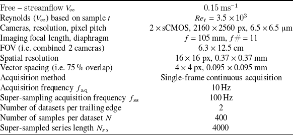
Table 2 Long description
The table presents a detailed summary of the experimental parameters used for flow-field measurements via planar particle image velocimetry (PIV). It includes specifications for the cameras, such as the type, resolution, and pixel pitch, which are two sCMOS cameras with a resolution of 2160 by 2560 pixels and a pixel pitch of 6.5 micrometers. The imaging focal length is 105 millimeters with a diaphragm setting of 11, covering a field of view (FOV) of 6.3 by 12.5 centimeters when combining both cameras. The spatial resolution is 16 by 16 pixels, equivalent to 0.37 by 0.37 millimeters, and the vector spacing, with a 75 percent overlap, is 4 by 4 pixels, or 0.095 by 0.095 millimeters. The acquisition method is single-frame continuous acquisition at a frequency of 10 hertz, with a super-sampling acquisition frequency of 100 hertz. Each dataset consists of 400 samples, and there are two datasets per trailing edge, resulting in a super-sampled series length of 4000.
Flow statistics in Section 3.1 were obtained by averaging both fields combined over the original maximum number of samples per trailing edge, corresponding to $2N$
. However, with a convective velocity proportional to the free stream of
$2N$
. However, with a convective velocity proportional to the free stream of ${0.15}\,\textrm {m s}^{-1}$
, the most energetic flow structures approximately shift by 1 cm between each image pair, corresponding to approximately 1/10th of the combined FOV. An advection-based model was employed to enhance the time resolution of the flow by super-sampling the vector-field dataset by a factor of 10, following the method described in Scarano and Moore (Reference Scarano and Moore2012). Using two datasets per trailing edge with super-sampling at a frequency of 1.2 Hz, we can ensure spectra are built with a cumulative total of more than 60 cycles at the shedding frequency and more than 150 cycles in the Strouhal number range of interest. The resulting time series are used as an input to compute the velocity material derivative and the pressure gradient. The contributions of the viscous stresses, despite being negligible in this work, close to the trailing edge are included in the material derivative formulation. The pressure reconstruction methodology is derived from previous studies by the authors, based on the material derivative of the flow velocity (Ragni et al. Reference Ragni, Avallone, van der Velden and Casalino2019). For the interested reader, in this study, the pressure gradient formulation is implemented in Lagrangian form, and the material derivative of the velocity is estimated by least-squares fitting of the velocities along a reconstructed particle trajectory. Two main changes are introduced with respect to the formulation from Pröbsting et al. (Reference Pröbsting, Scarano, Bernardini and Pirozzoli2013): the time stencil used to evaluate the material derivative employed a total of 5 vector fields (i.e. reference
${0.15}\,\textrm {m s}^{-1}$
, the most energetic flow structures approximately shift by 1 cm between each image pair, corresponding to approximately 1/10th of the combined FOV. An advection-based model was employed to enhance the time resolution of the flow by super-sampling the vector-field dataset by a factor of 10, following the method described in Scarano and Moore (Reference Scarano and Moore2012). Using two datasets per trailing edge with super-sampling at a frequency of 1.2 Hz, we can ensure spectra are built with a cumulative total of more than 60 cycles at the shedding frequency and more than 150 cycles in the Strouhal number range of interest. The resulting time series are used as an input to compute the velocity material derivative and the pressure gradient. The contributions of the viscous stresses, despite being negligible in this work, close to the trailing edge are included in the material derivative formulation. The pressure reconstruction methodology is derived from previous studies by the authors, based on the material derivative of the flow velocity (Ragni et al. Reference Ragni, Avallone, van der Velden and Casalino2019). For the interested reader, in this study, the pressure gradient formulation is implemented in Lagrangian form, and the material derivative of the velocity is estimated by least-squares fitting of the velocities along a reconstructed particle trajectory. Two main changes are introduced with respect to the formulation from Pröbsting et al. (Reference Pröbsting, Scarano, Bernardini and Pirozzoli2013): the time stencil used to evaluate the material derivative employed a total of 5 vector fields (i.e. reference $\pm$
2 or
$\pm$
2 or $n=\,$
2), and a polynomial of order
$n=\,$
2), and a polynomial of order $m=\,$
2 is chosen (i.e. a second-order approximation of the flow curvature) for the Lagrangian fit of the vector fields to compute the material derivative. The previous choices were verified to give converged results for the time spectra. The pressure is integrated by setting up a Poisson problem, and by solving the linear system of equations obtained by a second-order accurate central-difference scheme in a preconditioned iterative method (with a 5-point stencil, which was found to be optimal for similar problems, see: Charonko et al. (Reference Charonko, King, Smith and Vlachos2010), Ragni et al. (Reference Ragni, Ashok, van Oudheusden and Scarano2009) and van Oudheusden (Reference van Oudheusden2013)). Boundary conditions are imposed on the normal components of the pressure gradient. In particular, Neumann boundary conditions are applied along the entire domain except at the top of the boundary layer, where a Dirichlet boundary condition is applied. The latter is obtained by imposing Bernoulli’s equation, using the ambient pressure and the free-stream velocity. The Dirichlet condition is set to the wall-normal location of 0.2
$m=\,$
2 is chosen (i.e. a second-order approximation of the flow curvature) for the Lagrangian fit of the vector fields to compute the material derivative. The previous choices were verified to give converged results for the time spectra. The pressure is integrated by setting up a Poisson problem, and by solving the linear system of equations obtained by a second-order accurate central-difference scheme in a preconditioned iterative method (with a 5-point stencil, which was found to be optimal for similar problems, see: Charonko et al. (Reference Charonko, King, Smith and Vlachos2010), Ragni et al. (Reference Ragni, Ashok, van Oudheusden and Scarano2009) and van Oudheusden (Reference van Oudheusden2013)). Boundary conditions are imposed on the normal components of the pressure gradient. In particular, Neumann boundary conditions are applied along the entire domain except at the top of the boundary layer, where a Dirichlet boundary condition is applied. The latter is obtained by imposing Bernoulli’s equation, using the ambient pressure and the free-stream velocity. The Dirichlet condition is set to the wall-normal location of 0.2 $\delta$
in a manner similar to that of Ghaemi et al. (Reference Ghaemi, Ragni and Scarano2012), which showed a negligible effect on the calculated wall pressure and a more accurate representation of the relatively larger velocity fluctuations.
$\delta$
in a manner similar to that of Ghaemi et al. (Reference Ghaemi, Ragni and Scarano2012), which showed a negligible effect on the calculated wall pressure and a more accurate representation of the relatively larger velocity fluctuations.
2.3. Uncertainty on velocity and pressure fluctuations
For the analysis, we start with the main sources of uncertainty in the velocity computed from this set-up: peak locking, finite spatial resolution and cross-correlation sampling uncertainties. Errors due to peak locking are negligible due to the relatively larger particle size employed. With a digital resolution of ${32.7}\,{\textrm {px mm}}^{-1}$
, a magnification factor of 0.22 and a diaphragm aperture of 11, the imaged particle on the sensor is approximately 17.4
${32.7}\,{\textrm {px mm}}^{-1}$
, a magnification factor of 0.22 and a diaphragm aperture of 11, the imaged particle on the sensor is approximately 17.4 $\unicode{x03BC}$
m (Adrian & Yao Reference Adrian and Yao1985), corresponding to approximately 2.5 px on the sensor. This eliminates peak-locking effects, as was also a posteriori verified by plotting the histogram of the round-off values of the particle vector displacements. Errors due to modulation by finite spatial resolution are indirectly estimated by assuming that a multi-pass cross-correlation algorithm featuring window deformation requires the length scales of flow structures to be modulated by less than 5 % to be larger than 1.7 times the window size (Schrijer & Scarano Reference Schrijer and Scarano2008). By using a window size of 0.37
$\unicode{x03BC}$
m (Adrian & Yao Reference Adrian and Yao1985), corresponding to approximately 2.5 px on the sensor. This eliminates peak-locking effects, as was also a posteriori verified by plotting the histogram of the round-off values of the particle vector displacements. Errors due to modulation by finite spatial resolution are indirectly estimated by assuming that a multi-pass cross-correlation algorithm featuring window deformation requires the length scales of flow structures to be modulated by less than 5 % to be larger than 1.7 times the window size (Schrijer & Scarano Reference Schrijer and Scarano2008). By using a window size of 0.37 $\,\times \,$
0.37 mm, flow structures as small as 0.6 mm can be measured with a 95 % accuracy. Random errors are mainly due to the cross-correlation algorithm. Considering that for the uncertainty the number of samples used for averaging of the single combined fields is 400 at 10 Hz, random errors on the mean velocity fields are
$\,\times \,$
0.37 mm, flow structures as small as 0.6 mm can be measured with a 95 % accuracy. Random errors are mainly due to the cross-correlation algorithm. Considering that for the uncertainty the number of samples used for averaging of the single combined fields is 400 at 10 Hz, random errors on the mean velocity fields are $\epsilon _{u,rand}=\sigma _{u}/\sqrt {N}$ $\approx {0.54}\,\textrm {mm s}^{-1}$
. Similarly, the uncertainty in the streamwise velocity fluctuations is
$\approx {0.54}\,\textrm {mm s}^{-1}$
. Similarly, the uncertainty in the streamwise velocity fluctuations is $\epsilon _{u',rand}=\sigma _{u}/\sqrt {2(N-1)}\approx {0.39}\,\textrm {mm s}^{-1}$
. The uncertainty analysis for the reconstructed pressure builds upon the work of Ghaemi et al. (Reference Ghaemi, Ragni and Scarano2012), Violato et al. (Reference Violato, Moore and Scarano2011) and de Kat and van Oudheusden (Reference de Kat and van Oudheusden2012). It begins by evaluating the systematic error, primarily caused by the acceleration between the velocity fields. For the formulation, we refer to the formula as in Boillot and Prasad (Reference Boillot and Prasad1996) corrected by a factor
$\epsilon _{u',rand}=\sigma _{u}/\sqrt {2(N-1)}\approx {0.39}\,\textrm {mm s}^{-1}$
. The uncertainty analysis for the reconstructed pressure builds upon the work of Ghaemi et al. (Reference Ghaemi, Ragni and Scarano2012), Violato et al. (Reference Violato, Moore and Scarano2011) and de Kat and van Oudheusden (Reference de Kat and van Oudheusden2012). It begins by evaluating the systematic error, primarily caused by the acceleration between the velocity fields. For the formulation, we refer to the formula as in Boillot and Prasad (Reference Boillot and Prasad1996) corrected by a factor $1/2$
to consider the effect of symmetric window deformation as in Ghaemi et al. (Reference Ghaemi, Ragni and Scarano2012)
$1/2$
to consider the effect of symmetric window deformation as in Ghaemi et al. (Reference Ghaemi, Ragni and Scarano2012)
 \begin{align} \epsilon _{u,sys}=\frac {1}{4} S\Delta t^2\left |\frac {D\boldsymbol{v}}{Dt}\right | , \end{align}
where S is the digital resolution of the system ${32.7}\,\textrm {px mm}^{-1}$
and
${32.7}\,\textrm {px mm}^{-1}$
and $|D{\boldsymbol{v}}/Dt|$
is the Lagrangian acceleration magnitude obtained by processing multiple vector fields with a time separation
$|D{\boldsymbol{v}}/Dt|$
is the Lagrangian acceleration magnitude obtained by processing multiple vector fields with a time separation $\Delta t$
. In the present study, adopting the original
$\Delta t$
. In the present study, adopting the original $\Delta t$
pertaining to the original time series at 10 Hz would be too conservative and inconsistent with the computation of the material derivative. According to the study by Scarano and Moore (Reference Scarano and Moore2012), a super-sampling factor of approximately 10 yields a 2 % increase in velocity error. An additional noise averaging process in frequency is introduced, resulting in a fivefold increase in time resolution. Although this does not affect data at lower frequencies, it was established at a much lower resolution and dynamic velocity range because a high-speed system was used in the study. Therefore, assuming the
$\Delta t$
pertaining to the original time series at 10 Hz would be too conservative and inconsistent with the computation of the material derivative. According to the study by Scarano and Moore (Reference Scarano and Moore2012), a super-sampling factor of approximately 10 yields a 2 % increase in velocity error. An additional noise averaging process in frequency is introduced, resulting in a fivefold increase in time resolution. Although this does not affect data at lower frequencies, it was established at a much lower resolution and dynamic velocity range because a high-speed system was used in the study. Therefore, assuming the $\Delta t$
value associated with a super-sampled 100 Hz frequency for the uncertainty evaluation and considering a 2 % increase on the value, with a measured acceleration magnitude below
$\Delta t$
value associated with a super-sampled 100 Hz frequency for the uncertainty evaluation and considering a 2 % increase on the value, with a measured acceleration magnitude below ${200}\,\textrm {mm s}^{-2}$
in the shear layer, the systematic error in the velocity fields is estimated to be approximately 5
${200}\,\textrm {mm s}^{-2}$
in the shear layer, the systematic error in the velocity fields is estimated to be approximately 5 $\unicode{x03BC}$
m corresponding to 0.16 px. Assuming that the Poisson integration does not add significant error to the pressure evaluation, we follow the procedure of Ghaemi et al. (Reference Ghaemi, Ragni and Scarano2012) by computing the root-mean-square (r.m.s.) of the pressure error from the Navier–Stokes equation, neglecting the viscous term as
$\unicode{x03BC}$
m corresponding to 0.16 px. Assuming that the Poisson integration does not add significant error to the pressure evaluation, we follow the procedure of Ghaemi et al. (Reference Ghaemi, Ragni and Scarano2012) by computing the root-mean-square (r.m.s.) of the pressure error from the Navier–Stokes equation, neglecting the viscous term as
 \begin{align} \epsilon _{p}\approx \rho \ ds \, \epsilon _{L,rand} \, = \rho \,ds \left (\epsilon _{L,trunc}+\epsilon _{L, vel}\right )=\rho \, ds\left (\frac {1}{2} S (n\Delta t)^2\left |\frac {D\boldsymbol{v}}{Dt}\right |\frac {\left |\nabla \cdot \boldsymbol{v}\right |}{\Delta t}+\frac {\epsilon _{u,rand}}{2 n\Delta t} \right ), \end{align}
where $ds$
is the PIV vector resolution. The estimate from the previous equation contains errors due to truncation of the material derivative in the Lagrangian tracking and to random errors in the velocity field. In the present work, the Lagrangian derivative truncation error is higher in the fluctuating shear-layer region. The circle of uncertainty in locating the fluid element at the next time step is, for this study,
$ds$
is the PIV vector resolution. The estimate from the previous equation contains errors due to truncation of the material derivative in the Lagrangian tracking and to random errors in the velocity field. In the present work, the Lagrangian derivative truncation error is higher in the fluctuating shear-layer region. The circle of uncertainty in locating the fluid element at the next time step is, for this study, $c_r=\frac {1}{2}S(n\Delta t)^{2}$
= 1.3 px or equivalently 0.04 mm. With a typical conservative value of
$c_r=\frac {1}{2}S(n\Delta t)^{2}$
= 1.3 px or equivalently 0.04 mm. With a typical conservative value of ${5}\,\textrm {s}^{-1}$
for the divergence in the field and a random velocity error assumed as above to be 0.1 px, the overall error due to truncation and random components for the pressure is 0.08 Pa (to be noted, assuming the density of the water as above
${5}\,\textrm {s}^{-1}$
for the divergence in the field and a random velocity error assumed as above to be 0.1 px, the overall error due to truncation and random components for the pressure is 0.08 Pa (to be noted, assuming the density of the water as above ${998.6}\,\textrm {kg m}^{-3}$
and n = 2). However, the use of a planar PIV set-up for flow-pressure reconstruction requires further discussion of the effect of three-dimensional (3-D) flow. Although the paper’s methodology for retrieving the dynamic permeability response is based on measurements taken in proximity to the object, the reader should consider that the presence of out-of-plane velocity gradients in its wake creates an additional source of error. Following the work of McClure and Yarusevych (Reference McClure and Yarusevych2017), the main indicator for assessing the importance of errors due to 3-D effects is again the divergence of the velocity field. If the flow is well represented by the 2-D gradients, then the velocity field’s divergence should be zero, or, equivalently, the residual values should be small relative to the reference gradient across the sample. In figure 2, we have employed the same approach and computed the statistical contribution of the divergence normalised by the characteristic gradient in the flow. The super-sampling procedure operates on planar 2-D velocity fields and does not introduce additional 3-D effects beyond those already present in the measured data; equivalently, the 3-D influence on super-sampling is not a major concern for this study. According to the study by McClure and Yarusevych (Reference McClure and Yarusevych2017), an error of up to approximately 20 % in pressure due to 3-D flow can be expected in the far part of the wake compared with the 2-D value based on their fit, while in the region where the pressure is extracted for the dynamic permeability, 3-D effects are less important and the error is approximately 5 % of the dynamic pressure.
${998.6}\,\textrm {kg m}^{-3}$
and n = 2). However, the use of a planar PIV set-up for flow-pressure reconstruction requires further discussion of the effect of three-dimensional (3-D) flow. Although the paper’s methodology for retrieving the dynamic permeability response is based on measurements taken in proximity to the object, the reader should consider that the presence of out-of-plane velocity gradients in its wake creates an additional source of error. Following the work of McClure and Yarusevych (Reference McClure and Yarusevych2017), the main indicator for assessing the importance of errors due to 3-D effects is again the divergence of the velocity field. If the flow is well represented by the 2-D gradients, then the velocity field’s divergence should be zero, or, equivalently, the residual values should be small relative to the reference gradient across the sample. In figure 2, we have employed the same approach and computed the statistical contribution of the divergence normalised by the characteristic gradient in the flow. The super-sampling procedure operates on planar 2-D velocity fields and does not introduce additional 3-D effects beyond those already present in the measured data; equivalently, the 3-D influence on super-sampling is not a major concern for this study. According to the study by McClure and Yarusevych (Reference McClure and Yarusevych2017), an error of up to approximately 20 % in pressure due to 3-D flow can be expected in the far part of the wake compared with the 2-D value based on their fit, while in the region where the pressure is extracted for the dynamic permeability, 3-D effects are less important and the error is approximately 5 % of the dynamic pressure.
(a) Instantaneous normalised divergence field for the baseline configuration; (b) standard deviation of the divergence field as computed from the turbulent statistics; (c) percentage error on pressure according to the fit from McClure and Yarusevych (Reference McClure and Yarusevych2017).
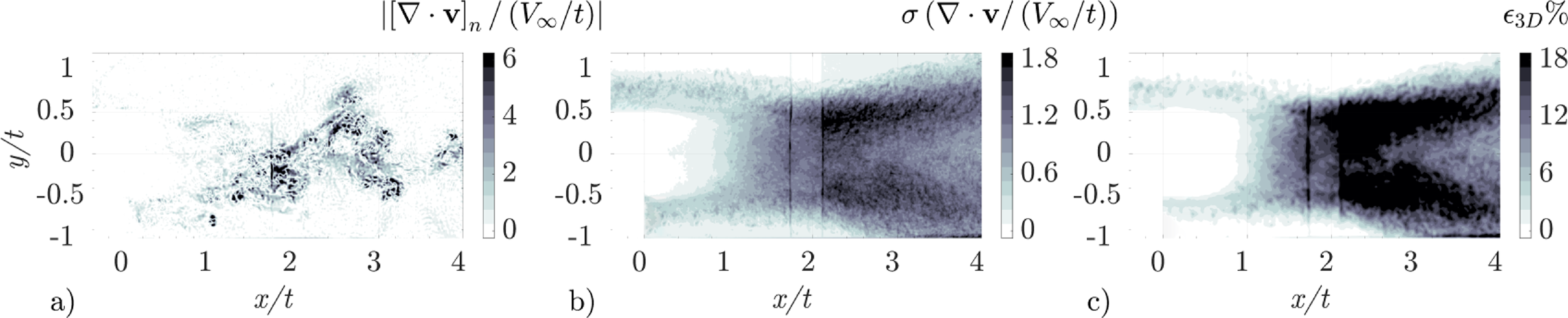
Figure 2 Long description
A heat map displays three different visualizations related to fluid dynamics. The first panel shows the instantaneous normalized divergence field for a baseline configuration, with varying intensities represented by different shades of gray. The second panel illustrates the standard deviation of the divergence field, computed from turbulent statistics, using a gradient from light to dark shades to indicate varying levels of deviation. The third panel presents the percentage error on pressure according to a specific fit, with a color scale ranging from light to dark shades to represent different error magnitudes. Each panel has axes labeled with ‘x over t’ and ‘y over t’, indicating normalized spatial dimensions over time. The color intensity in each panel highlights regions of interest, such as areas of high divergence, significant standard deviation, or notable pressure error.
3. Turbulent wake analysis
3.1. Flow statistics
The mean wake flow statistics of the solid trailing edge (STE), SPTE and RFTE are plotted in figure 3. In this manuscript, we focus purely on the communication effects of the permeable materials. Therefore, more information on the specific aerodynamic performance in terms of momentum-deficit reduction will be omitted, and for the interested reader, it can be found in another study by the same authors (Arcondoulis et al. Reference Arcondoulis, Ragni, Fiscaletti and Merino-Martinez2025). The turbulent statistics are obtained by averaging the original 2 datasets, each containing 400 images. This also applies to the pressure field, which, after processing for the super-sampled dataset, is downsampled again to the original two 400-image series, for consistency. The convergence of the down-sampled series is verified by monitoring the standard deviation as a function of the number of acquired samples, which is omitted for brevity. The STE in figure 3a–c shows a symmetrical distribution of the streamwise velocity component, as determined by a region of momentum deficit extending to approximately $x/t\approx$
2. After this location, the momentum deficit begins to recover. The wakes behind the SPTE and the RFTE exhibit a shorter momentum deficit, as can be seen by comparing figure 3d–f with figure 3g–i. Compared with the STE, the momentum deficit develops over a shorter downstream distance (to
$x/t\approx$
2. After this location, the momentum deficit begins to recover. The wakes behind the SPTE and the RFTE exhibit a shorter momentum deficit, as can be seen by comparing figure 3d–f with figure 3g–i. Compared with the STE, the momentum deficit develops over a shorter downstream distance (to $ x/t \approx$
1.5). The mean vertical-velocity component confirms the previous observation. Two regions characterised by approximately 10 %-magnitude vertical-velocity components with opposite signs can be identified at approximately
$ x/t \approx$
1.5). The mean vertical-velocity component confirms the previous observation. Two regions characterised by approximately 10 %-magnitude vertical-velocity components with opposite signs can be identified at approximately $x/t=\,$
[1.2, 0.9, 0.8] for the STE, SPTE and RFTE, respectively, indicating a shorter shedding length for the permeable materials and consequently a faster momentum-deficit recovery. The pressure contours in figures 3c, 3f and 3i follow the averaged velocity components. The contours are normalised by the free-stream pressure
$x/t=\,$
[1.2, 0.9, 0.8] for the STE, SPTE and RFTE, respectively, indicating a shorter shedding length for the permeable materials and consequently a faster momentum-deficit recovery. The pressure contours in figures 3c, 3f and 3i follow the averaged velocity components. The contours are normalised by the free-stream pressure $p_\infty$
and by the dynamic pressure
$p_\infty$
and by the dynamic pressure $1/2\rho V_{\infty }^2$
. The pressure coefficient contours show that the pressure recovers at the maximum extension of the momentum-deficit region. Since the pressure coefficient is found to recover to zero in the FOV for all configurations, it can be concluded that the wake entrainment is fully captured. To verify that the faster recovery of the two porous trailing edges is due to the alteration of the vortex shedding coherence due to permeability, the following section is dedicated to the analysis of the spatio-temporal characteristics of the vortex shedding.
$1/2\rho V_{\infty }^2$
. The pressure coefficient contours show that the pressure recovers at the maximum extension of the momentum-deficit region. Since the pressure coefficient is found to recover to zero in the FOV for all configurations, it can be concluded that the wake entrainment is fully captured. To verify that the faster recovery of the two porous trailing edges is due to the alteration of the vortex shedding coherence due to permeability, the following section is dedicated to the analysis of the spatio-temporal characteristics of the vortex shedding.
Normalised time-averaged velocity components, $\overline {u}/V_{\infty }$
and
$\overline {u}/V_{\infty }$
and $\overline {v}/V_{\infty }$
, and normalised time-averaged pressure field,
$\overline {v}/V_{\infty }$
, and normalised time-averaged pressure field, $(\overline {p}-p_{\infty })/q_{\infty }$
for the STE (a–c), structured porous trailing edge SPTE (d–f) and randomised foam trailing edge RFTE (g–i). Flow is from left to right.
$(\overline {p}-p_{\infty })/q_{\infty }$
for the STE (a–c), structured porous trailing edge SPTE (d–f) and randomised foam trailing edge RFTE (g–i). Flow is from left to right.
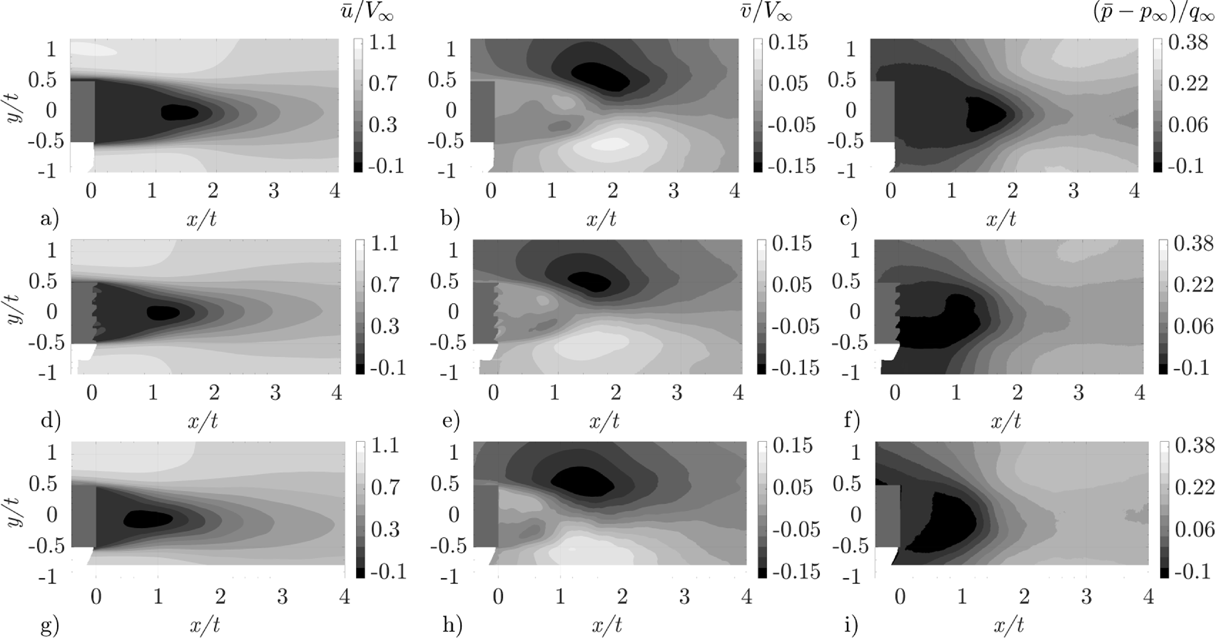
Figure 3 Long description
A heat map displays normalized time-averaged velocity components and pressure fields for three different trailing edge designs: STE, SPTE, and RFTE. The flow direction is from left to right. The heat map is divided into three rows, each representing a different trailing edge design. Each row contains three subplots: the first subplot shows the normalized time-averaged velocity component in the x-direction, the second subplot shows the normalized time-averaged velocity component in the y-direction, and the third subplot shows the normalized time-averaged pressure field. The color scale for the velocity components ranges from -0.1 to 1.1, with lighter colors indicating higher values and darker colors indicating lower values. The color scale for the pressure field ranges from -0.1 to 0.38, with lighter colors indicating higher values and darker colors indicating lower values. The heat map reveals distinct patterns and variations in velocity and pressure fields for each trailing edge design.
Figure 4 presents the r.m.s. of the fluctuations of the streamwise velocity, vertical velocity and pressure coefficient, for the STE in figure 4a–c, SPTE in figure 4d–f and RFTE in figure 4g–i. The results align with previous studies focusing on permeable materials for the attenuation of Karman vortex instabilities (e.g. Maryami et al. (Reference Maryami, Arcondoulis, Liu and Liu2023)), also identifying the location of the beginning of the flow entrainment in the wake with the location where the maximum standard deviation of the velocity components is recorded (Roshko Reference Roshko1954). Figure 4 further illustrates the enhanced attenuation of vortex shedding achieved by the porous materials compared with the STE. In particular, both SPTE and RFTE present lower r.m.s. values than STE across all velocity components, and the location of the respective maximum fluctuations is closer to the trailing-edge location for both porous materials. The contours from the STE, in the top panels of figure 4, show that the maximum fluctuation values are localised at approximately $x/t\lessapprox 2$
, consistent with the location at which the wake recovery starts, analogous to the profile distribution from previous studies by Nakamura (Reference Nakamura1996) and Okajima (Reference Okajima1982). By comparing the different materials with respect to the straight trailing edge, an approximately 10 % reduction is observed for the SPTE and RFTE compared with the STE. As also analysed in a study by the same authors (Arcondoulis et al. Reference Arcondoulis, Ragni, Fiscaletti and Merino-Martinez2025), the rearrangement of the Reynolds stresses in the wake is facilitated by the tendency of porous materials to create velocity oscillations that alter the Reynolds stress profile along the material thickness. Concurrently, this creates a more rapid recovery of the momentum deficit in the wake, determined by the positive ‘flow communication’ between the boundary layer and the wake regions (as also seen in previous studies by Koh et al. (Reference Koh, Meinke and Schröder2018) and Showkat Ali et al. (Reference Showkat Ali, Azarpeyvand and Ilário da Silva2020)). In particular, the flow communication entails a non-negligible velocity correlation in fluid regions separated by the object.
$x/t\lessapprox 2$
, consistent with the location at which the wake recovery starts, analogous to the profile distribution from previous studies by Nakamura (Reference Nakamura1996) and Okajima (Reference Okajima1982). By comparing the different materials with respect to the straight trailing edge, an approximately 10 % reduction is observed for the SPTE and RFTE compared with the STE. As also analysed in a study by the same authors (Arcondoulis et al. Reference Arcondoulis, Ragni, Fiscaletti and Merino-Martinez2025), the rearrangement of the Reynolds stresses in the wake is facilitated by the tendency of porous materials to create velocity oscillations that alter the Reynolds stress profile along the material thickness. Concurrently, this creates a more rapid recovery of the momentum deficit in the wake, determined by the positive ‘flow communication’ between the boundary layer and the wake regions (as also seen in previous studies by Koh et al. (Reference Koh, Meinke and Schröder2018) and Showkat Ali et al. (Reference Showkat Ali, Azarpeyvand and Ilário da Silva2020)). In particular, the flow communication entails a non-negligible velocity correlation in fluid regions separated by the object.
Normalised r.m.s. of velocity components, $u'/V_{\infty }$
,
$u'/V_{\infty }$
, $v'/V_{\infty }$
and pressure fluctuations,
$v'/V_{\infty }$
and pressure fluctuations, $p'/q_{\infty }$
, for the STE (a–c), SPTE (d–f) and RFTE (g–i). Flow is from left to right, and
$p'/q_{\infty }$
, for the STE (a–c), SPTE (d–f) and RFTE (g–i). Flow is from left to right, and $q_{\infty }$
is calculated as 1/2
$q_{\infty }$
is calculated as 1/2 $\rho V_\infty ^2$
.
$\rho V_\infty ^2$
.
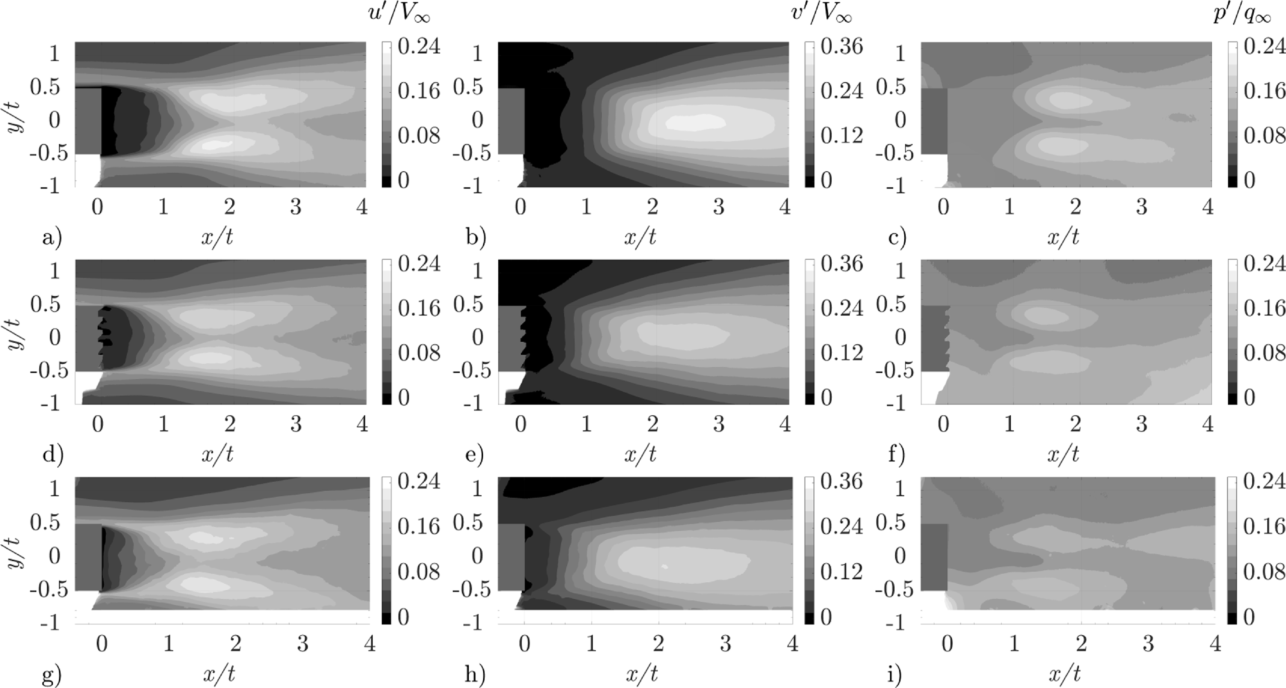
Figure 4 Long description
A heat map displays the normalized root mean square of velocity components and pressure fluctuations for three different flow conditions: STE, SPTE, and RFTE. The flow direction is from left to right. The heat map is divided into three rows, each representing a different flow condition. Each row contains three subplots showing the normalized root mean square of the velocity components u’ and v’ and the pressure fluctuations p’. The x-axis represents the normalized streamwise distance (x/t), and the y-axis represents the normalized transverse distance (y/t). The color scale indicates the magnitude of the normalized root mean square values, with lighter colors representing higher values and darker colors representing lower values. The range of values for u’ and p’ is from 0 to 0.24, and for v’ it is from 0 to 0.36. The heat map shows distinct patterns and regions of high and low values, indicating the distribution and intensity of velocity and pressure fluctuations in the wake of bluff bodies under different flow conditions.
3.2. Unsteady-flow features
In this section, attention is drawn to three regions: the boundary layer, the shear layer generated at the trailing edge and the deeper wake flow. Spectra of the vorticity and pressure signals are computed from the super-sampled time-resolved flow field at the three aforementioned locations corresponding to P1(–0.20, 0.60), P2(1, 0.5), P3(2, 0), and depicted by red marks in figure 5. The left column of figure 5 presents maps of instantaneous non-dimensionalised vorticity magnitude for the (a) STE, (d) SPTE and (g) RFTE, to assist the visualisation of the flow field at the three selected points. Panels in the middle and right columns of figure 5 are auto-spectra of vorticity and pressure fluctuations calculated at the three locations. The spectra of both vorticity and pressure fluctuations at P1 show a relatively broadband distribution, consistent with the turbulent frequency distribution of a fully developed boundary layer. The distribution of the SPTE presents a lower-frequency content (i.e. $St$
< 1) with respect to both STE and RFTE, possibly due to the interaction of flow scales at the pore level with the SPTE geometry (Arcondoulis et al. Reference Arcondoulis, Ragni, Fiscaletti and Merino-Martinez2025). For all configurations, the maximum energy content remains centred in the range
$St$
< 1) with respect to both STE and RFTE, possibly due to the interaction of flow scales at the pore level with the SPTE geometry (Arcondoulis et al. Reference Arcondoulis, Ragni, Fiscaletti and Merino-Martinez2025). For all configurations, the maximum energy content remains centred in the range $St$
= [0.2–1], with no relevant peak observed at the shedding frequency
$St$
= [0.2–1], with no relevant peak observed at the shedding frequency $St$
= 0.2 at the P1 locations. Since the characteristics of the incoming boundary layer are very similar across the three cases, the auto-spectral distributions of both vorticity and pressure are similarly broadband before separating at the edge. Further downstream at P2, both the permeable and solid trailing edges exhibit a narrow-band contribution centred on the shedding frequency in the vorticity and pressure auto-spectra. More precisely, the spectral contribution from the vortex shedding can be seen to be building up already at
$St$
= 0.2 at the P1 locations. Since the characteristics of the incoming boundary layer are very similar across the three cases, the auto-spectral distributions of both vorticity and pressure are similarly broadband before separating at the edge. Further downstream at P2, both the permeable and solid trailing edges exhibit a narrow-band contribution centred on the shedding frequency in the vorticity and pressure auto-spectra. More precisely, the spectral contribution from the vortex shedding can be seen to be building up already at $x/t$
= 1; at a Strouhal number of 0.2 based on the thickness
$x/t$
= 1; at a Strouhal number of 0.2 based on the thickness $t$
, corresponding to approximately
$t$
, corresponding to approximately $f$
= 1.2 Hz, the pressure spectra of both configurations exhibit a peak. Both permeable materials mitigate vortex shedding, as evidenced by the lower peak values at
$f$
= 1.2 Hz, the pressure spectra of both configurations exhibit a peak. Both permeable materials mitigate vortex shedding, as evidenced by the lower peak values at $St$
= 0.2, consistent with the literature (Geyer Reference Geyer2020). A secondary peak at
$St$
= 0.2, consistent with the literature (Geyer Reference Geyer2020). A secondary peak at $St$
= 1 (
$St$
= 1 ( $f$
= 6 Hz) is observed for the SPTE, which is not visible for the RFTE, originating from the element size of the structured porous insert. The spectra at P3 reveal a relatively broadband distribution for both SPTE and RFTE, while the STE still shows peaks at
$f$
= 6 Hz) is observed for the SPTE, which is not visible for the RFTE, originating from the element size of the structured porous insert. The spectra at P3 reveal a relatively broadband distribution for both SPTE and RFTE, while the STE still shows peaks at $St$
= 0.2 and its harmonic
$St$
= 0.2 and its harmonic $St$
= 0.4, due to the scalar nature of the pressure fluctuations, which do not distinguish between co- and counter-rotating vorticity. It is also important to comment on the high-frequency harmonics in the pressure spectra. This series of harmonics, at a multiple of 10 Hz (
$St$
= 0.4, due to the scalar nature of the pressure fluctuations, which do not distinguish between co- and counter-rotating vorticity. It is also important to comment on the high-frequency harmonics in the pressure spectra. This series of harmonics, at a multiple of 10 Hz ( $St$
= 1.7), corresponds to the acquisition frequency of the cameras from which the super-sampled time series is created. Since the super-sampling process propagates the vector fields back and forth from the instantaneous series at a low repetition rate, a change in the masked series of vectors determines a small change in the boundary conditions of the pressure fluctuation, recorded as noise at that specific frequency.
$St$
= 1.7), corresponds to the acquisition frequency of the cameras from which the super-sampled time series is created. Since the super-sampling process propagates the vector fields back and forth from the instantaneous series at a low repetition rate, a change in the masked series of vectors determines a small change in the boundary conditions of the pressure fluctuation, recorded as noise at that specific frequency.
Left column: maps of normalised instantaneous vorticity, $|\omega |t/V_{\infty }$
, and the positions of three points (P1, P2 and P3) at which auto-spectra are calculated for the (a) STE, (d) SPTE and (g) RFTE. Flow is from left to right. Middle and right columns: auto-spectra of vorticity,
$|\omega |t/V_{\infty }$
, and the positions of three points (P1, P2 and P3) at which auto-spectra are calculated for the (a) STE, (d) SPTE and (g) RFTE. Flow is from left to right. Middle and right columns: auto-spectra of vorticity, $\Phi _{\omega \omega }$
and pressure fluctuations,
$\Phi _{\omega \omega }$
and pressure fluctuations, $\Phi _{pp}$
, calculated at P1, P2, P3, for (b, c) the STE, (e, f) the SPTE and (h, i) the RFTE. Note the uncertainty in the velocity and pressure field varying in the FOV in paragraph 2.3.
$\Phi _{pp}$
, calculated at P1, P2, P3, for (b, c) the STE, (e, f) the SPTE and (h, i) the RFTE. Note the uncertainty in the velocity and pressure field varying in the FOV in paragraph 2.3.

Figure 5 Long description
The image contains three sets of graphs. The left column shows maps of normalized instantaneous vorticity with three points (P1, P2, and P3) marked for each of the STE, SPTE, and RFTE. The middle and right columns display auto-spectra of vorticity and pressure fluctuations calculated at these points. Each set of graphs corresponds to different flow conditions: STE, SPTE, and RFTE. The flow direction is from left to right. The auto-spectra graphs show the variations in vorticity and pressure fluctuations at the specified points for each condition. The uncertainty in the velocity and pressure fields varies within the field of view.
4. Flow communication through permeable materials
Before deriving the dynamic permeability function, this section demonstrates how flow propagates through the material. We first quantify this flow communication using velocity correlations. Proper orthogonal decomposition (POD) is then employed to further isolate and visualise the dominant regions where this communication occurs. By separating coherent flow structures, POD highlights how different materials influence the spatial distribution of flow penetration. Accordingly, the first part of the section presents the velocity-correlation analysis, while the second part shows how regions of strong POD-identified flow communication provide insight into the material’s dynamic permeability response.
4.1. Spectral analysis of velocity and vorticity
Maps of instantaneous vorticity together with the spectral analysis of the vorticity and the magnitude-squared coherence of the vertical-velocity fluctuations (i.e. magnitude of $C_{v,v}$
) and the wall-normal velocity fluctuations (i.e. magnitude of
$C_{v,v}$
) and the wall-normal velocity fluctuations (i.e. magnitude of $C_{v,u}$
) are presented in figure 6. The results for the STE are presented in the top row, the SPTE results in the middle row and the RFTE results in the bottom row. The spectral analysis of the vortical fluctuations is performed by plotting the power spectral density at different locations within the middle column. While the point in the boundary layer is kept the same as before, now indicated by P4(−0.20, 0.60), new points are chosen and analysed in the direct proximity of the sample wall: P5(0.05, 0.40), P6(0.05, 0.35), P7(0.05, 0.30), P8(0.05, 0.25). The point distribution is chosen to highlight the energy content of fluctuations near the sample trailing edges compared with those in the boundary layer. Starting from the STE, the energy content of the vortical fluctuations in the wake of the object (points P5–P8) is negligible with respect to the vorticity content in the boundary layer (point P4), as can be seen in figure 6b. The magnitude-squared coherence in figure 6c shows very low correlation between the vertical flow fluctuations in the boundary layer and those just behind the sample thickness for both vertical and normal components. This is consistent with the fact that, since the STE is non-permeable, the flow velocity in the separated region at the trailing edge approaches zero. Therefore, velocity fluctuations in the boundary layer are mostly shielded by the separated region and convected downstream. Comparing the results with figure 6e, the SPTE shows relatively higher content of the flow fluctuations at the same locations in the wake, mostly below
$C_{v,u}$
) are presented in figure 6. The results for the STE are presented in the top row, the SPTE results in the middle row and the RFTE results in the bottom row. The spectral analysis of the vortical fluctuations is performed by plotting the power spectral density at different locations within the middle column. While the point in the boundary layer is kept the same as before, now indicated by P4(−0.20, 0.60), new points are chosen and analysed in the direct proximity of the sample wall: P5(0.05, 0.40), P6(0.05, 0.35), P7(0.05, 0.30), P8(0.05, 0.25). The point distribution is chosen to highlight the energy content of fluctuations near the sample trailing edges compared with those in the boundary layer. Starting from the STE, the energy content of the vortical fluctuations in the wake of the object (points P5–P8) is negligible with respect to the vorticity content in the boundary layer (point P4), as can be seen in figure 6b. The magnitude-squared coherence in figure 6c shows very low correlation between the vertical flow fluctuations in the boundary layer and those just behind the sample thickness for both vertical and normal components. This is consistent with the fact that, since the STE is non-permeable, the flow velocity in the separated region at the trailing edge approaches zero. Therefore, velocity fluctuations in the boundary layer are mostly shielded by the separated region and convected downstream. Comparing the results with figure 6e, the SPTE shows relatively higher content of the flow fluctuations at the same locations in the wake, mostly below $St\,\approx \,2$
. The magnitude-squared coherence in figure 6f also shows stronger similarity of the vertical flow fluctuations in a range below
$St\,\approx \,2$
. The magnitude-squared coherence in figure 6f also shows stronger similarity of the vertical flow fluctuations in a range below $St\,\approx \,1$
with respect to the fluctuations in the boundary layer. Relatively lower is the similarity of the wall-normal components for the two locations, which are still non-negligible in the same frequency range of the vertical flow fluctuations. Relatively higher fluctuations of vorticity with respect to the STE are additionally measured for the RFTE in figure 6h, although of lower value than those of the SPTE, possibly due to the smaller uniform pore size in all directions within the material. This dampening effect of fluctuations with relatively lower frequencies is also confirmed by the magnitude-squared coherence of both vertical and wall-normal components in figure 6i, which resembles that of the STE, albeit with slightly higher similarity in the low-frequency range. The presence of vortical flow structures with velocity fluctuations similar to those in the boundary layer for permeable materials can be taken as indirect evidence of flow communication, which is predominantly observed at
$St\,\approx \,1$
with respect to the fluctuations in the boundary layer. Relatively lower is the similarity of the wall-normal components for the two locations, which are still non-negligible in the same frequency range of the vertical flow fluctuations. Relatively higher fluctuations of vorticity with respect to the STE are additionally measured for the RFTE in figure 6h, although of lower value than those of the SPTE, possibly due to the smaller uniform pore size in all directions within the material. This dampening effect of fluctuations with relatively lower frequencies is also confirmed by the magnitude-squared coherence of both vertical and wall-normal components in figure 6i, which resembles that of the STE, albeit with slightly higher similarity in the low-frequency range. The presence of vortical flow structures with velocity fluctuations similar to those in the boundary layer for permeable materials can be taken as indirect evidence of flow communication, which is predominantly observed at $St\,\lt \,1$
for both permeable materials. The differences in the magnitude-squared coherence between the SPTE and RFTE can be attributed to the distinct structures of the two materials, with the SPTE promoting communication at frequencies proportional to its pore size. By additionally investigating the spectral content across points from P5 to P8 for SPTE and RFTE, it can be observed that, while the RFTE shows a nearly identical distribution across points, the SPTE spectral content decreases with increasing distance from the boundary layer. This is an effect of the channel distribution in the SPTE: the farther from the boundary layer, the greater the pressure losses imposed on the flow, which dissipate the vortical fluctuations along the paths. An aspect common to the two porous materials is that flow fluctuations with higher-frequency responses corresponding to flow structures smaller than half the pore size do not obviously correlate with each other over the measured distance, since they are dissipated before. This means that for
$St\,\lt \,1$
for both permeable materials. The differences in the magnitude-squared coherence between the SPTE and RFTE can be attributed to the distinct structures of the two materials, with the SPTE promoting communication at frequencies proportional to its pore size. By additionally investigating the spectral content across points from P5 to P8 for SPTE and RFTE, it can be observed that, while the RFTE shows a nearly identical distribution across points, the SPTE spectral content decreases with increasing distance from the boundary layer. This is an effect of the channel distribution in the SPTE: the farther from the boundary layer, the greater the pressure losses imposed on the flow, which dissipate the vortical fluctuations along the paths. An aspect common to the two porous materials is that flow fluctuations with higher-frequency responses corresponding to flow structures smaller than half the pore size do not obviously correlate with each other over the measured distance, since they are dissipated before. This means that for $St$
> 2, no correlation can be effectively measured.
$St$
> 2, no correlation can be effectively measured.
Maps of vorticity magnitude in the left column superimposed to the locations of the one point in the boundary layer P4, and four points in the wake, P5–P8, at which the spectral density (middle column) of vorticity and the magnitude-squared coherence (right column) of both the vertical and wall-normal velocity components as extracted from the points are computed for (a–c) the STE, (d–f) the SPTE and (g–i) the RFTE. We note that P4 corresponds to P1 in figure 5. Additionally, the wall-normal components are plotted mirrored with a second axis on the right of the graph, pointing downward.

Figure 6 Long description
The image contains three sets of graphs, each with three columns. The left column shows vorticity magnitude maps superimposed with the locations of five points (P4, P5, P6, P7, P8) for three different trailing edges: STE, SPTE, and RFTE. The middle column displays the spectral density of vorticity at these points. The right column presents the magnitude-squared coherence of both the vertical and wall-normal velocity components, with the wall-normal components mirrored and plotted with a second axis on the right, pointing downward. The graphs compare the structured porous trailing edge (SPTE) and the randomised foam trailing edge (RFTE) with a solid trailing-edge baseline, highlighting differences in permeability decay rates and coherent flow communication bandwidths.
4.2. Proper orthogonal decomposition
Despite yielding key insights into the flow communication process, the spectra presented in figures 5 and 6 do not provide quantitative indications of the spatio-temporal convection of the flow structures involved in the process and their organisation. Further clarification of these aspects can be obtained by visualising the velocity fluctuations in the boundary layer and the near-field region of the wake. To retain exclusively the velocity fluctuations expected within the flow communication, a filtering procedure based on POD is applied (Berkooz et al. Reference Berkooz, Holmes and Lumley1993; Lumley Reference Lumley1967). The distribution of the normalised eigenvalues pertaining to the POD mode decomposition of the velocity fields for all materials is computed. The eigenvalue distribution in figure 7a for the STE is shown for reference, since the ones for RFTE and SPTE follow a very similar trend. It is verified that the modes with the eigenvalue distribution in figure 7a can be divided into three ranges. The first range of high-energy modes corresponds to flow structures of the same size as the vortex shedding, and their energy decays logarithmically with increasing POD modes (blue dashed line). The intermediate range corresponds to the convective regime of the high-frequency structures, marking a change in slope in the graph (red dashed line). The last region with relatively low-energy content contains flow structures from wake mixing and the residual of the decomposition (black dashed line). A low-order reconstruction from the POD mode decomposition is computed in the region of the change of slope. The higher-energy modes are intentionally neglected to isolate the high-frequency distribution of flow structures that can be convected through the permeable materials in the vicinity of the recirculation region. The reconstructed velocity and vorticity fields are presented in figure 7. In particular, the reconstructed velocity and vorticity fields are presented for the STE in figures 7b and 7c, for the SPTE in figures 7d and 7e and for the RFTE in figures 7f and 7g.
Low-order reconstruction of one super-sampled time series based upon POD based on its singular value decomposition, in the range $n={300\lt n\lt 700}$
as shown in (a) for the STE (b, c), SPTE (d, e) and RFTE (f, g). The fluctuations of velocity are reconstructed for one of the frames in fields b–d–f, and the vorticity ones in c–e–g. The modal energy distribution in (a) is presented only for the STE, since the SPTE and RFTE ones are very similar.
$n={300\lt n\lt 700}$
as shown in (a) for the STE (b, c), SPTE (d, e) and RFTE (f, g). The fluctuations of velocity are reconstructed for one of the frames in fields b–d–f, and the vorticity ones in c–e–g. The modal energy distribution in (a) is presented only for the STE, since the SPTE and RFTE ones are very similar.

Figure 7 Long description
The image contains multiple graphs analyzing low-order reconstruction of velocity and vorticity fields for different trailing edge configurations. The first graph (a) shows the modal energy distribution for the STE (Structured Porous Trailing Edge). The subsequent graphs (b, c, d, e, f, g) display the reconstructed velocity and vorticity fields for the STE, SPTE (Structured Porous Trailing Edge), and RFTE (Randomised Foam Trailing Edge) configurations. Graphs b, d, and f illustrate the velocity fluctuations, while graphs c, e, and g depict the vorticity fluctuations. The x-axis represents the spatial coordinate x divided by the thickness t, and the y-axis represents the spatial coordinate y divided by the thickness t. The color bars indicate the magnitude of the velocity and vorticity fluctuations. The modal energy distribution in graph (a) is specific to the STE, as the SPTE and RFTE configurations exhibit similar distributions.
In figures 7b and 7c, the low-order reconstruction is shown for the STE. By observing the velocity components and vorticity fluctuations, a stagnation region can be identified behind the STE. The fluctuations with high spatial frequency from the boundary layer are convected directly downstream to $x/t \approx 1$
. Due to the non-permeability of the trailing edge, very low amplitude residuals of large fluctuations can be measured in the recirculation region. Figures 7d and 7e present the same distribution for the SPTE. A clear difference in mixing is observed with vortical flow structures seeping through the porosity. The low-order reconstruction also shows high-spatial-frequency fluctuations, proportional to the cell-unit size, permeating the material. Due to the pore dimensions, fluctuations with spatial dimensions below the millimetre level are more prominent. These correspond to a Strouhal number of approximately 1, assuming a convective velocity through the material approximately one tenth that of the boundary layer. In figures 7f and 7g, the comparison is extended to the trailing edge of the randomised foam. The uniform, equally distributed pore size in the randomised foam results in a clear increase in the high-frequency fluctuations in the wake region. Fluctuations with a spatial dimension larger than the pore size are statistically uniformly distributed in the wake region due to the pore size of the randomised foam, supporting the previous conclusions from figure 6.
$x/t \approx 1$
. Due to the non-permeability of the trailing edge, very low amplitude residuals of large fluctuations can be measured in the recirculation region. Figures 7d and 7e present the same distribution for the SPTE. A clear difference in mixing is observed with vortical flow structures seeping through the porosity. The low-order reconstruction also shows high-spatial-frequency fluctuations, proportional to the cell-unit size, permeating the material. Due to the pore dimensions, fluctuations with spatial dimensions below the millimetre level are more prominent. These correspond to a Strouhal number of approximately 1, assuming a convective velocity through the material approximately one tenth that of the boundary layer. In figures 7f and 7g, the comparison is extended to the trailing edge of the randomised foam. The uniform, equally distributed pore size in the randomised foam results in a clear increase in the high-frequency fluctuations in the wake region. Fluctuations with a spatial dimension larger than the pore size are statistically uniformly distributed in the wake region due to the pore size of the randomised foam, supporting the previous conclusions from figure 6.
4.3. Transfer function evaluation from the unsteady-flow data
In this section, a lumped-model approach is proposed to evaluate the dynamic response of permeability in porous materials subjected to grazing flows. The approach enables direct assessment of the material’s unsteady response from flow information, thereby extending conventional approaches. The time-averaged parameters are typically obtained by curve fitting the experimental pressure drop in a channel with a uniform section, based on the Hazen–Dupuit–Darcy equation (Geyer Reference Geyer2020; Narasimhan Reference Narasimhan2013; Rubio-Carpio et al. Reference Rubio-Carpio, Merino-Martínez, Avallone, Ragni, Sneller and van der Zwaag2019). The approach of this study relates the unsteady response of velocity fluctuations to the unsteady pressure gradient, comparing the results with the theoretical model proposed by Johnson et al. (Reference Johnson, Koplik and Dashen1987). To describe the lumped-system approach, a schematic is presented in figure 8a is proposed. The problem is simplified by considering only the neighbouring pressure at the points P $_{A}$
and P
$_{A}$
and P $_{C}$
. Clearly, points farther from the object are not considered in the system, as they can be assimilated to an equivalent impedance in the AB direction, providing a contribution that is already accounted for in the circuit. When considering one side of the circuit, the points P
$_{C}$
. Clearly, points farther from the object are not considered in the system, as they can be assimilated to an equivalent impedance in the AB direction, providing a contribution that is already accounted for in the circuit. When considering one side of the circuit, the points P $_{A}$
and P
$_{A}$
and P $_{C}$
are either connected through a fluid impedance when considering the solid STE case in figure 8a, or both through fluid and material paths. The circuit analogy stands behind the fact that, if we consider the permeable material, an incompressible stream tube (i.e. density,
$_{C}$
are either connected through a fluid impedance when considering the solid STE case in figure 8a, or both through fluid and material paths. The circuit analogy stands behind the fact that, if we consider the permeable material, an incompressible stream tube (i.e. density, $\rho$
, is constant) with momentum flux
$\rho$
, is constant) with momentum flux $\rho A_{A}V_{A}$
is split in P
$\rho A_{A}V_{A}$
is split in P $_{A}$
into two components, a contribution
$_{A}$
into two components, a contribution $\rho A_{m}v_{m}$
through the material path AA”, and a remaining one
$\rho A_{m}v_{m}$
through the material path AA”, and a remaining one $\rho A_{f}v_{f}$
through the fluid path AB. The terms
$\rho A_{f}v_{f}$
through the fluid path AB. The terms $v_{m}$
and
$v_{m}$
and $v_{f}$
are respectively the velocity at the material interface and convected along AB, while
$v_{f}$
are respectively the velocity at the material interface and convected along AB, while $A_{n}$
and
$A_{n}$
and $A_{f}$
are respectively the interfacial area through the material and the one perpendicular to the fluid path. The same pressure differential is established between the same nodal points. To describe the material properties, the current study refers to the formulations of Cortis et al. (Reference Cortis, Smeulders, Guermond and Lafarge2003) and Johnson et al. (Reference Johnson, Koplik and Dashen1987), which were obtained by averaging the material properties over disturbances with wavelengths larger than the channel’s pore size. Additionally, for this specific application, we demonstrate that there is negligible communication along the path AA”A’ due to the material’s thickness with respect to the incoming boundary layer. The differential equations along the circuits are
$A_{f}$
are respectively the interfacial area through the material and the one perpendicular to the fluid path. The same pressure differential is established between the same nodal points. To describe the material properties, the current study refers to the formulations of Cortis et al. (Reference Cortis, Smeulders, Guermond and Lafarge2003) and Johnson et al. (Reference Johnson, Koplik and Dashen1987), which were obtained by averaging the material properties over disturbances with wavelengths larger than the channel’s pore size. Additionally, for this specific application, we demonstrate that there is negligible communication along the path AA”A’ due to the material’s thickness with respect to the incoming boundary layer. The differential equations along the circuits are
 \begin{align} \begin{cases} ABC: \quad \nabla p=\left [-\rho \left ( \frac {dv_{f}}{dt}+ v_{f}\frac {dv_{f}}{ds}\right )+\mu \frac {d^2 v_{f}}{ds^2}\right ] ,\\[6pt] AA''C: \quad \nabla p=-\mu \frac {\phi }{k(\omega )}v_m, \end{cases} \end{align}
where $\nabla p$
is the gradient of pressure through the indicated paths,
$\nabla p$
is the gradient of pressure through the indicated paths, $\phi$
is the open area or porosity,
$\phi$
is the open area or porosity, $K$
is the dynamic permeability and
$K$
is the dynamic permeability and $s$
is the path coordinate. For simplicity, all velocity contributions along the paths are averaged over their length. Of primary interest is the ratio of the pressure difference across the two points along the AC path to the velocity through the material, which determines the dynamic permeability experimentally. Here, the relationship between the exiting velocity and the measurement of unsteady pressure fluctuations at two different nodes of the material is targeted. As discussed by Cortis et al. (Reference Cortis, Smeulders, Guermond and Lafarge2003), by considering only the fluctuating part of the signal in the velocity and pressure gradient in (4.1), it is possible to frame an electrical analogy where the pressure differential is analogous to an equivalent circuit voltage. In this analogy, if the elements
$s$
is the path coordinate. For simplicity, all velocity contributions along the paths are averaged over their length. Of primary interest is the ratio of the pressure difference across the two points along the AC path to the velocity through the material, which determines the dynamic permeability experimentally. Here, the relationship between the exiting velocity and the measurement of unsteady pressure fluctuations at two different nodes of the material is targeted. As discussed by Cortis et al. (Reference Cortis, Smeulders, Guermond and Lafarge2003), by considering only the fluctuating part of the signal in the velocity and pressure gradient in (4.1), it is possible to frame an electrical analogy where the pressure differential is analogous to an equivalent circuit voltage. In this analogy, if the elements $\rho v_f$
and
$\rho v_f$
and $\rho v_m$
are assumed to be circuit currents, then the material branch of the circuit contributes with an equivalent resistance, while the fluid branch includes more complex equivalent impedance, which can be reformulated as equivalent inductance and capacitance.
$\rho v_m$
are assumed to be circuit currents, then the material branch of the circuit contributes with an equivalent resistance, while the fluid branch includes more complex equivalent impedance, which can be reformulated as equivalent inductance and capacitance.
Conceptual schematic diagram of (a) the lumped-system model for the STE (for reference), and (b) lumped-system model for the permeable trailing edge. The $Z$
-terms represent flow impedances connecting pressure points at different locations.
$Z$
-terms represent flow impedances connecting pressure points at different locations.

Figure 8 Long description
The image presents two conceptual schematic diagrams. The first diagram (a) illustrates the lumped-system model for the STE, featuring points labeled P_A, P_B, P_C, P_A’, and P_B’ connected by flow impedances Z_AB, Z_BC, Z_A’B’, and Z_B’C’. These points and impedances are arranged in a solid medium. The second diagram (b) depicts a lumped-system model for describing the response to flow fluctuations. It includes similar points and impedances but introduces additional impedances Z_AA’, Z_A’C’, and Z_A’C’ in a permeable medium. The diagrams highlight the flow impedances connecting pressure points at different locations, illustrating the differences between solid and permeable media in managing flow fluctuations.
To validate the approach, it is important to make sure that the fluxes through the material are consistent with the model presented above. For this analysis, it is possible to monitor, for a given pressure difference between the two nodes, the spatial distribution of the fluid velocity, which, when fed to (4.1), yields an approximation of the dynamic permeability, $k$
. In figure 9, the fluxes through the material are first plotted versus time in the corner region according to the convention shown above. In particular, due to the thickness
$k$
. In figure 9, the fluxes through the material are first plotted versus time in the corner region according to the convention shown above. In particular, due to the thickness $t$
of the porous sample, a
$t$
of the porous sample, a $t/2$
length is used to compute the vertical fluxes, with the horizontal length adjusted to maintain the same mass flow. It is verified that in the present study, comparable lengths along the horizontal direction balance the fluxes in the vertical direction. For materials with highly inhomogeneous porosity across different boundaries, the two lengths should be proportionally adjusted, since the assumption of mass flow conservation must be verified. Additionally, in the present study, the actual values of the normalised fluxes per unit area already converge from a
$t/2$
length is used to compute the vertical fluxes, with the horizontal length adjusted to maintain the same mass flow. It is verified that in the present study, comparable lengths along the horizontal direction balance the fluxes in the vertical direction. For materials with highly inhomogeneous porosity across different boundaries, the two lengths should be proportionally adjusted, since the assumption of mass flow conservation must be verified. Additionally, in the present study, the actual values of the normalised fluxes per unit area already converge from a $t/6$
length, which is consistent with the pore dimension size of the adopted materials. Those correspond to the flux that enters the material from element A in figure 9 and the outward flux exiting from the material, i.e. the outward element C in the same figure. The left figure pertains to the solid configuration, the middle figure to the SPTE, and the right to the RFTE. The plots confirm the presence of a non-negligible amount of incoming and outgoing flow for the permeable materials. The average entering and exiting mass fluxes at the top and lateral sides are found to have opposite signs, confirming that the flow enters from the boundary-layer sides and exits from the side exposed to the wake.
$t/6$
length, which is consistent with the pore dimension size of the adopted materials. Those correspond to the flux that enters the material from element A in figure 9 and the outward flux exiting from the material, i.e. the outward element C in the same figure. The left figure pertains to the solid configuration, the middle figure to the SPTE, and the right to the RFTE. The plots confirm the presence of a non-negligible amount of incoming and outgoing flow for the permeable materials. The average entering and exiting mass fluxes at the top and lateral sides are found to have opposite signs, confirming that the flow enters from the boundary-layer sides and exits from the side exposed to the wake.
Orientation of fluxes and their evaluation for the (a) STE, (b) SPTE and (c) RFTE. Note that the two super-sampled series are added one after the other in the plot.

Figure 9 Long description
The line graph consists of three subplots labeled Solid, SPTE, and RFTE, each showing the evaluation of fluxes over time. The x-axis represents time in seconds, ranging from 0 to 80 seconds. The y-axis represents the flux in milligrams per square millimeter per second, ranging from -50 to 50. Each subplot contains two data lines: one in red and one in blue. The red line represents the flux out, and the blue line represents the flux in. In the Solid subplot, both lines are relatively flat and close to zero, indicating minimal fluctuation. In the SPTE subplot, the lines show slight fluctuations around zero. In the RFTE subplot, the lines exhibit more noticeable fluctuations but remain centered around zero. The graph illustrates how the fluxes vary over time for different conditions, highlighting the differences in flux behavior between the Solid, SPTE, and RFTE evaluations. All values are approximated.
The velocity, $v_m$
, is computed at the direct exit of the permeable material, since the fluxes exiting the material exhibit a lower uncertainty than the incoming ones. In figure 10, the value of the normalised frequency-dependent response of permeability is computed by using the experimental data and compared with the theoretically expected behaviour from Johnson et al. (Reference Johnson, Koplik and Dashen1987). The analytical model is depicted in figure 10 in black and was derived using the uniform and homogeneous parameters in table 2. The experimental counterpart of the dynamic permeability is derived by averaging the velocity and the pressure difference over the previously indicated
$v_m$
, is computed at the direct exit of the permeable material, since the fluxes exiting the material exhibit a lower uncertainty than the incoming ones. In figure 10, the value of the normalised frequency-dependent response of permeability is computed by using the experimental data and compared with the theoretically expected behaviour from Johnson et al. (Reference Johnson, Koplik and Dashen1987). The analytical model is depicted in figure 10 in black and was derived using the uniform and homogeneous parameters in table 2. The experimental counterpart of the dynamic permeability is derived by averaging the velocity and the pressure difference over the previously indicated $t/2$
horizontal and vertical lengths. The pressure gradient is computed as the instantaneous difference of the spatially averaged pressure between the two horizontal and vertical sides of the corners. We remind the reader that the experimental values are obtained by using the second row of (4.1), once again normalised by the known parameters of table 2. Therefore, two different decays are derived for the two materials. The model also allows for extracting the equivalent tortuosity and the viscous length-scale values by overlapping the experimental response with the analytical one. Both measured curves compare with a very similar decay in frequency to the analytical formula from Johnson et al. (Reference Johnson, Koplik and Dashen1987), using the estimated parameters above. A slightly higher response is observed experimentally for the SPTE than for the RFTE; however, the values are very close. In particular, from the study of Johnson et al. (Reference Johnson, Koplik and Dashen1987), a tortuosity of between 2 and 4 should correspond to an arbitrary homogeneous and isotropic distribution of channels proportional to the pore size length. The extracted parameters are
$t/2$
horizontal and vertical lengths. The pressure gradient is computed as the instantaneous difference of the spatially averaged pressure between the two horizontal and vertical sides of the corners. We remind the reader that the experimental values are obtained by using the second row of (4.1), once again normalised by the known parameters of table 2. Therefore, two different decays are derived for the two materials. The model also allows for extracting the equivalent tortuosity and the viscous length-scale values by overlapping the experimental response with the analytical one. Both measured curves compare with a very similar decay in frequency to the analytical formula from Johnson et al. (Reference Johnson, Koplik and Dashen1987), using the estimated parameters above. A slightly higher response is observed experimentally for the SPTE than for the RFTE; however, the values are very close. In particular, from the study of Johnson et al. (Reference Johnson, Koplik and Dashen1987), a tortuosity of between 2 and 4 should correspond to an arbitrary homogeneous and isotropic distribution of channels proportional to the pore size length. The extracted parameters are $\Lambda =[0.5, 0.8]$
mm and
$\Lambda =[0.5, 0.8]$
mm and $\alpha _{\infty }=[2,3]$
respectively for the SPTE and for the RFTE. This is consistent with the derivation from Johnson et al. (Reference Johnson, Koplik and Dashen1987) showing that the viscous length scales should correspond to a fraction of the pore size. By combining the flow results with the dynamic-permeability analysis, we observe that the SPTE behaves with a higher permeability response than the RFTE at high frequency. These trends reflect the influence of the material’s internal architecture, which appears to restrict flow communication somewhat more than the RFTE at higher Strouhal numbers. Although the differences between the two materials are small, they are still meaningful: they help explain why the acoustic performances of the SPTE and RFTE are reported to be comparable (Arcondoulis et al. Reference Arcondoulis, Ragni, Fiscaletti, Merino-Martinez and Liu2024, Reference Arcondoulis, Ragni, Fiscaletti and Merino-Martinez2025), despite the SPTE exhibiting somewhat better aerodynamic drag performance and the RFTE showing a slightly faster wake recovery in the flow measurements.
$\alpha _{\infty }=[2,3]$
respectively for the SPTE and for the RFTE. This is consistent with the derivation from Johnson et al. (Reference Johnson, Koplik and Dashen1987) showing that the viscous length scales should correspond to a fraction of the pore size. By combining the flow results with the dynamic-permeability analysis, we observe that the SPTE behaves with a higher permeability response than the RFTE at high frequency. These trends reflect the influence of the material’s internal architecture, which appears to restrict flow communication somewhat more than the RFTE at higher Strouhal numbers. Although the differences between the two materials are small, they are still meaningful: they help explain why the acoustic performances of the SPTE and RFTE are reported to be comparable (Arcondoulis et al. Reference Arcondoulis, Ragni, Fiscaletti, Merino-Martinez and Liu2024, Reference Arcondoulis, Ragni, Fiscaletti and Merino-Martinez2025), despite the SPTE exhibiting somewhat better aerodynamic drag performance and the RFTE showing a slightly faster wake recovery in the flow measurements.
Dynamic permeability derived from the unsteady fluctuations using (4.1). The coloured lines are derived from time-resolved PIV, while the black lines are obtained from Johnson et al. (Reference Johnson, Koplik and Dashen1987). Fitted values for the SPTE and RFTE are respectively: $\Lambda =$
[0.5, 0.8] mm. Dashed curves are derived for
$\Lambda =$
[0.5, 0.8] mm. Dashed curves are derived for $\alpha _{\infty }$
= [2, 3].
$\alpha _{\infty }$
= [2, 3].

Figure 10 Long description
The line graph displays dynamic permeability derived from unsteady fluctuations. The colored lines represent data from time-resolved PIV, while the black lines are from Johnson et al. (1987). The fitted values for the SPTE and RFTE are respectively 0.5 and 0.8 millimeters. Dashed curves are derived for alpha infinity values of 2 and 3. The x-axis represents the Strouhal number (St), and the y-axis represents the normalized permeability (|k(omega)| / k0). The red line represents SPTE, the blue line represents RFTE, and the dashed black lines represent the fitted values for alpha infinity. All values are approximated.
5. Conclusions
A new experimental method is developed and demonstrated for measuring the dynamic permeability of porous trailing edges under grazing flow, based on time-resolved PIV and a lumped-system circuit analogy. Unlike conventional steady-flow rig measurements, this approach operates directly in the aerodynamic environment of interest and accommodates thin trailing-edge geometries. An experimental study using time-resolved PIV in water was conducted to investigate how materials with similar porous characteristics elicit different unsteady-flow responses. Depending on the internal flow path, locally correlated flow velocity fluctuations indicate that the scales of velocity fluctuations depend on the material’s inner parameters, which indirectly affect different flow frequencies with different response amplitudes. Mean results and fluctuations indicate that the integral effect of the flow communication determines a different outcome in the turbulent wake of the various materials. The spectra of both vorticity and pressure fluctuations transition from broadband to narrow-band, with communication across a range of Strouhal frequencies from approximately 0.2 to approximately 1. A method to quantify the effective response function of the material to velocity fluctuations is proposed, based on circuit analysis, which assumes a lumped system comprising different elements within the material. The approach enables the measurement and validation of the material’s dynamic-permeability response under grazing conditions and allows comparison with existing analytical response functions. At relatively higher Strouhal number, the measured permeability curves exhibit differences in decay slope between the SPTE and RFTE. These differences are consistent with the expectation that microstructural features, such as pore orientation and flow-path tortuosity, can influence the frequency response. While the present data do not isolate the specific mechanisms responsible, the observed trend suggests that internal architecture may play a role in shaping the high-frequency decay, warranting further targeted investigation. This methodology can be extended beyond trailing-edge noise control to a wide range of permeable bluff-body and porous-wall problems in fluid mechanics, such as ventilation in bio-inspired surfaces, flow control in turbomachinery or the characterisation of permeable sediment beds in environmental flows. Enabling in situ measurement of dynamic permeability under realistic operating conditions opens a pathway to rapidly linking material design parameters with their aerodynamic and acoustic performance.
Supplementary material
The supplementary material for this article can be found at https://doi.org/10.1017/flo.2026.10053.
Data availability statement
Raw data are available from the corresponding author.
Author contributions
D. R., D. F. and E. J. G. A. created the research plan, designed and performed the experiments. D. R. additionally wrote the manuscript, which has been reviewed multiple times by D. F. and E. J. G. A.
Funding statement
The authors acknowledge the Dutch Research Council (NWO) for financing the study under the Open Technology Program: Aeroacoustic Multi-path Permeable geometries for airfoil Edge noise REduction, AMPERE, TTW-OTP grant number 20467.
Competing interests
The authors declare no conflicts of interest.
Ethical standards
The research adheres to all ethical guidelines, including compliance with the legal requirements of the study country.
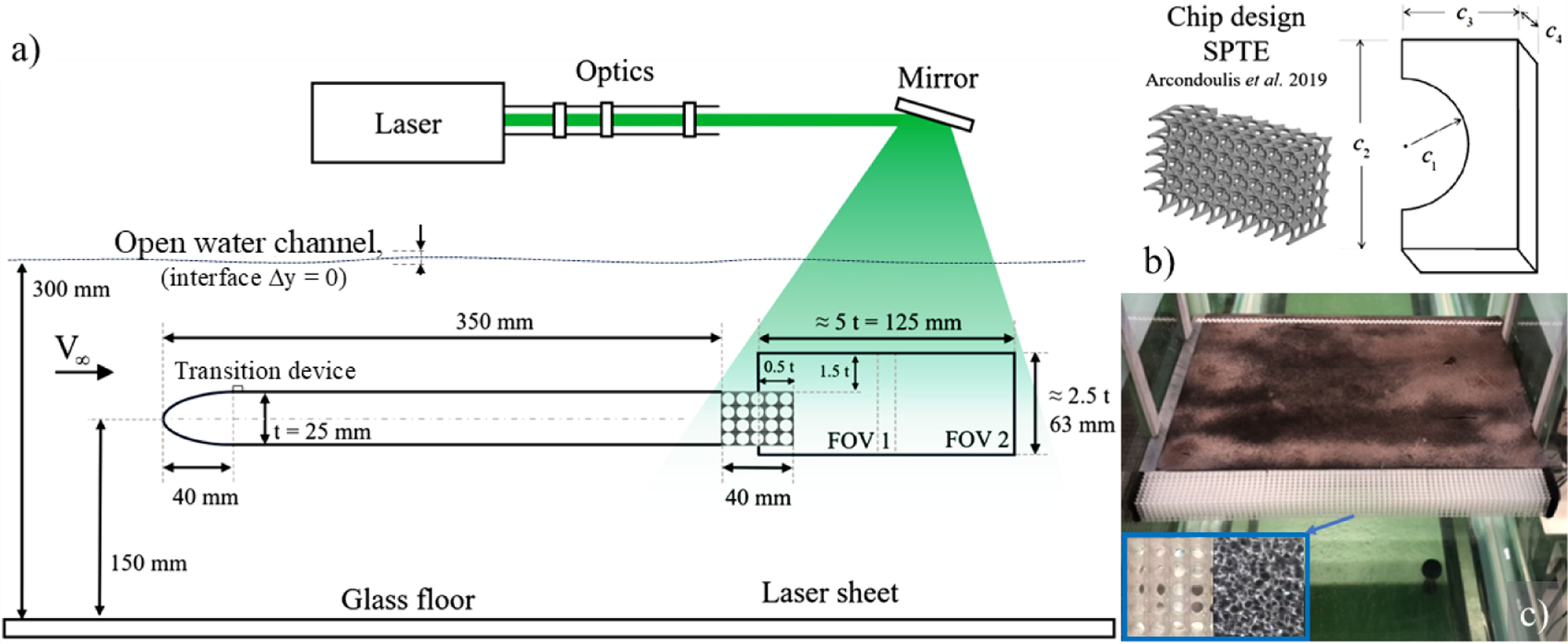

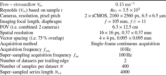
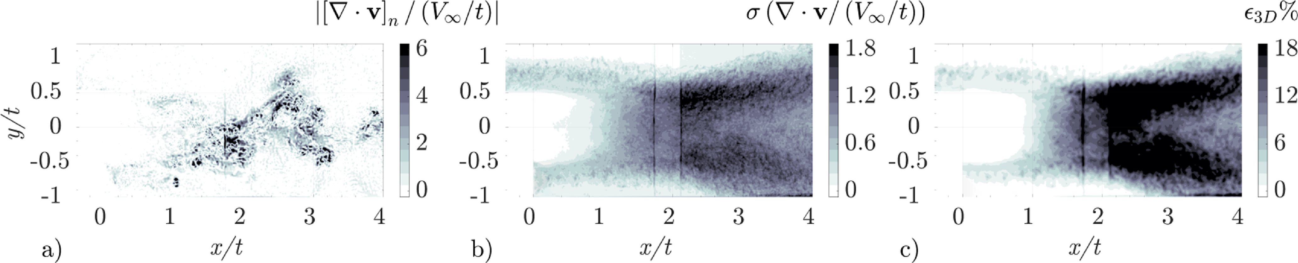
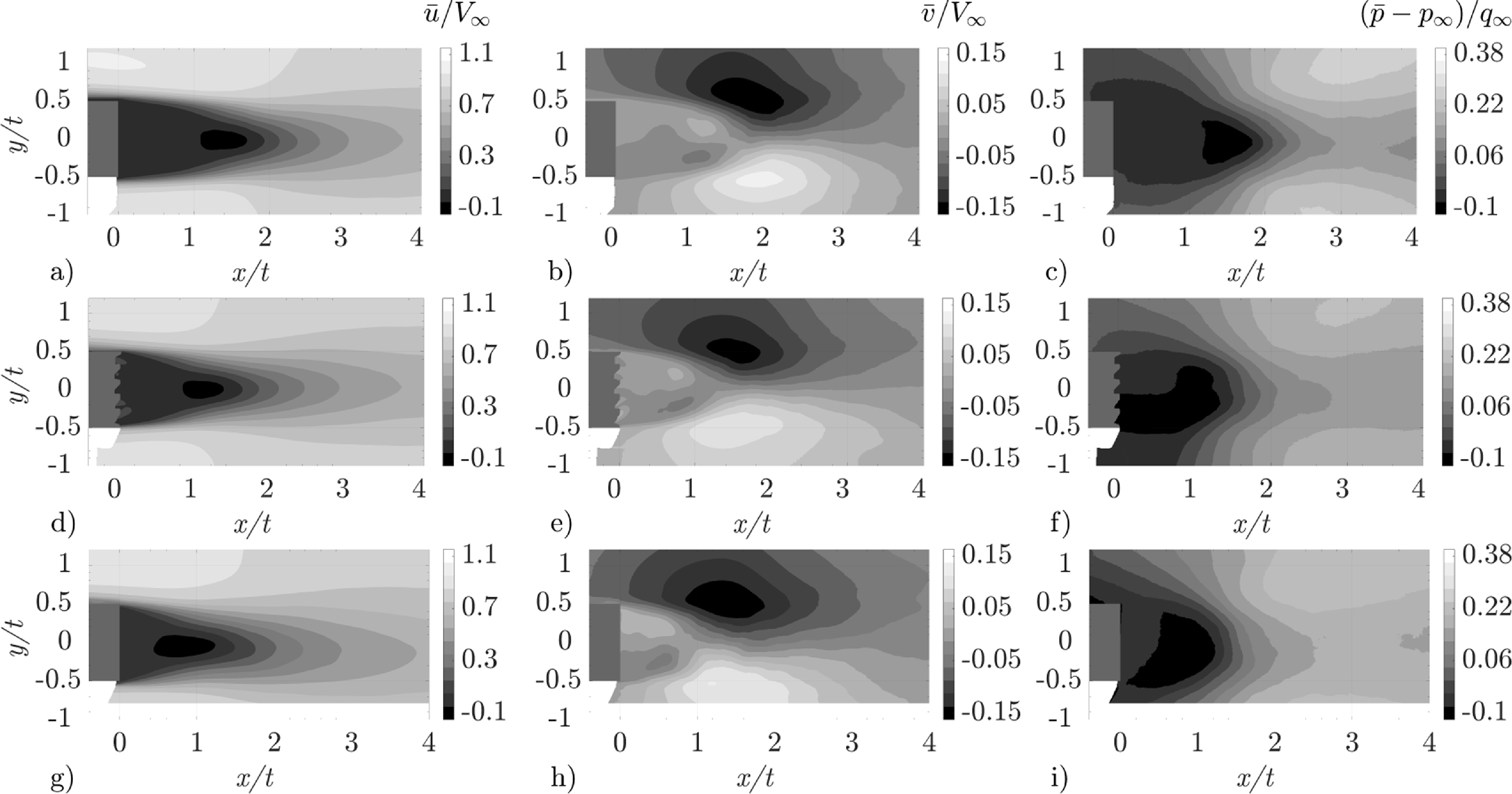
 u¯/V∞
u¯/V∞ v¯/V∞
v¯/V∞ (p¯−p∞)/q∞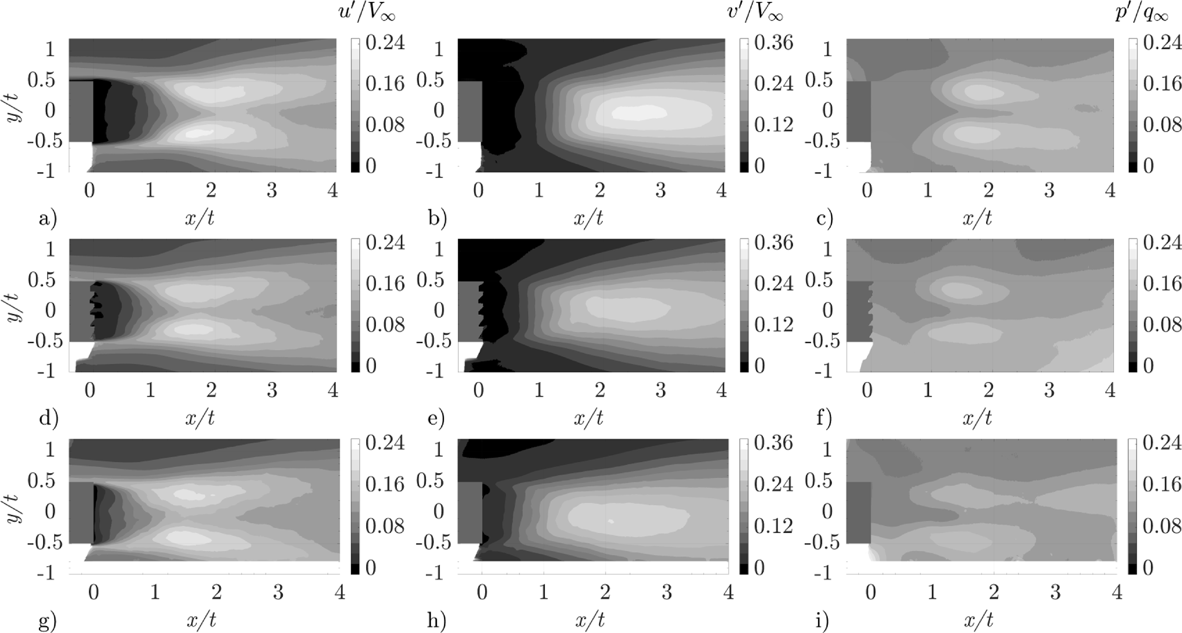
 u′/V∞
u′/V∞ v′/V∞
v′/V∞ p′/q∞
p′/q∞ q∞
q∞ ρV∞2
ρV∞2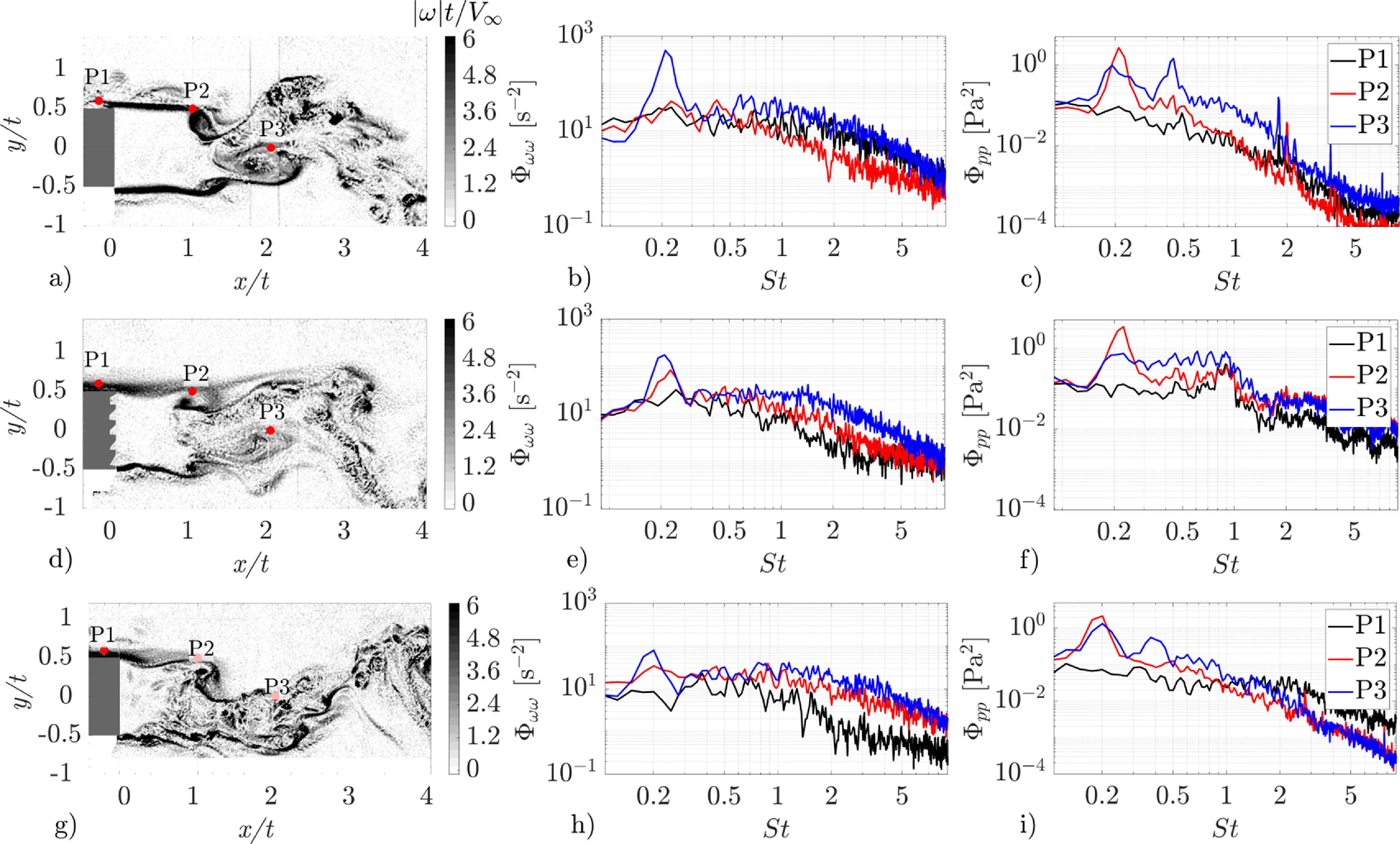
 |ω|t/V∞
 Φωω
Φωω Φpp
Φpp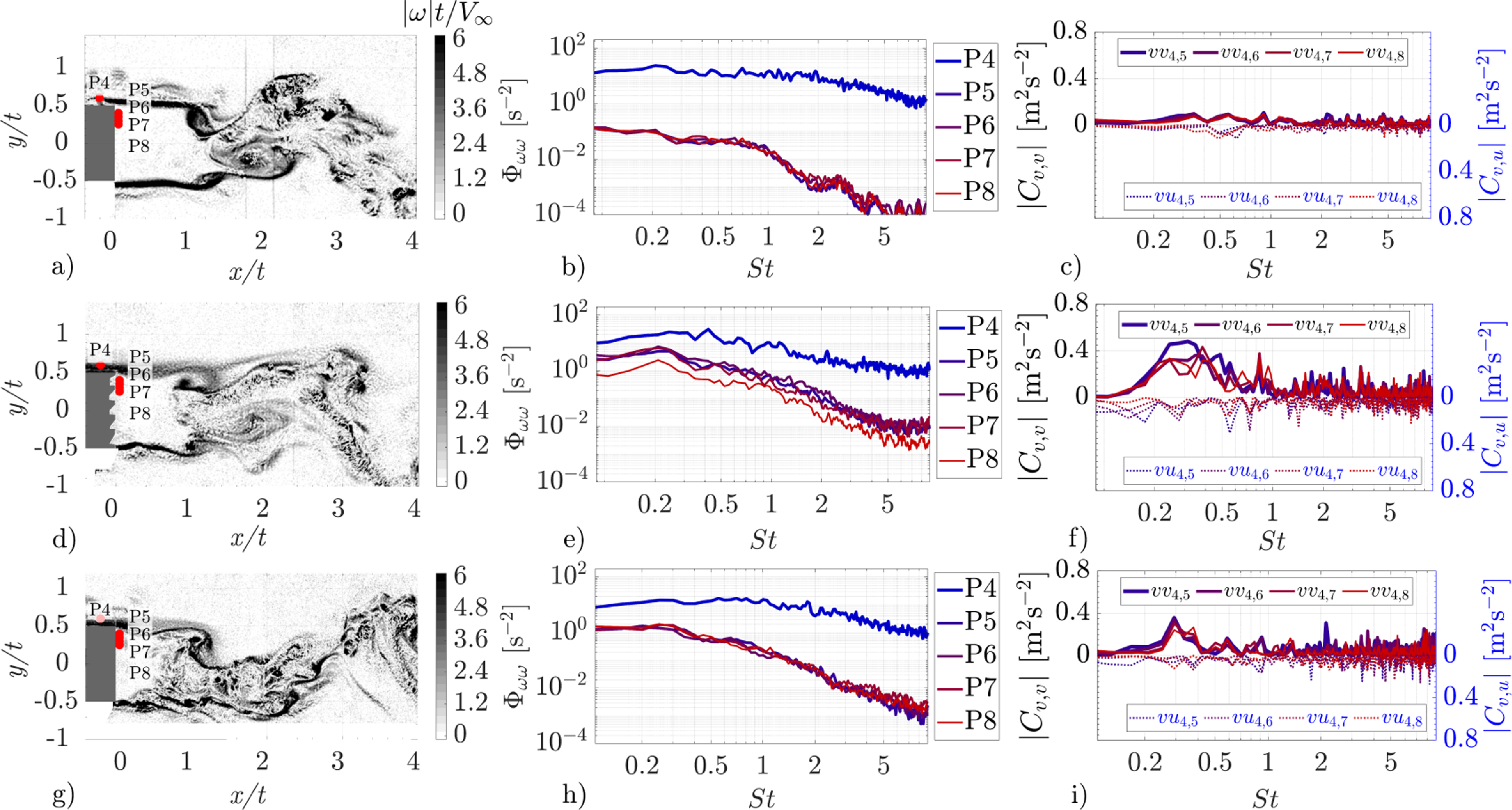
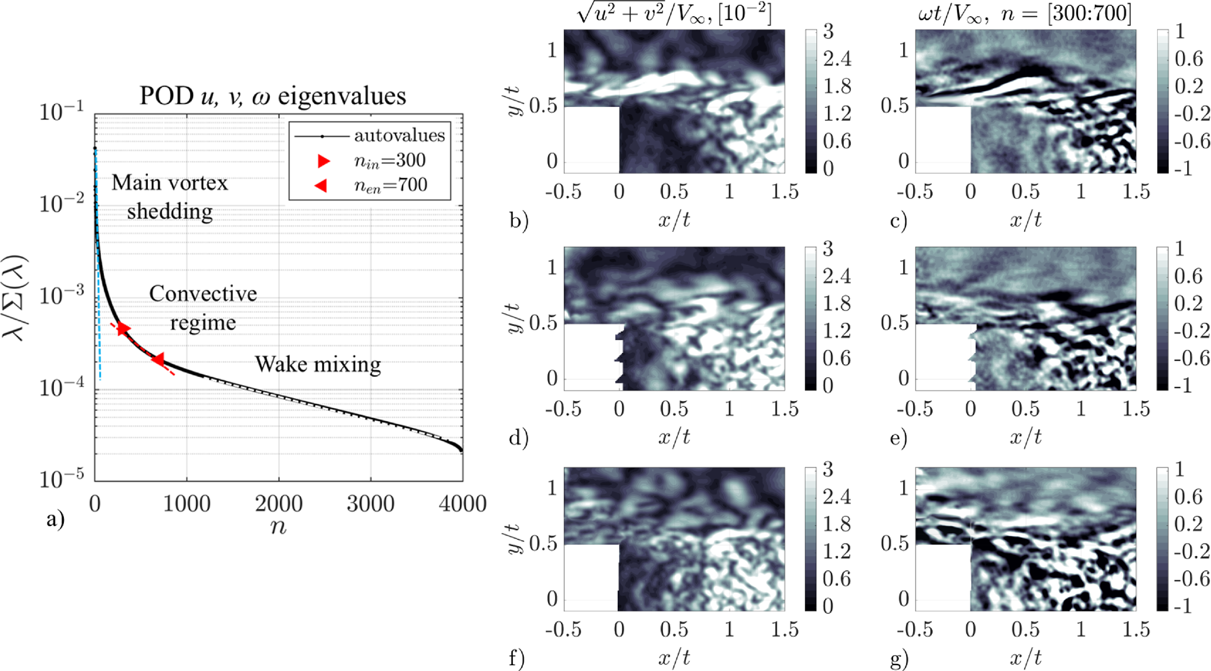
 n=300
n=300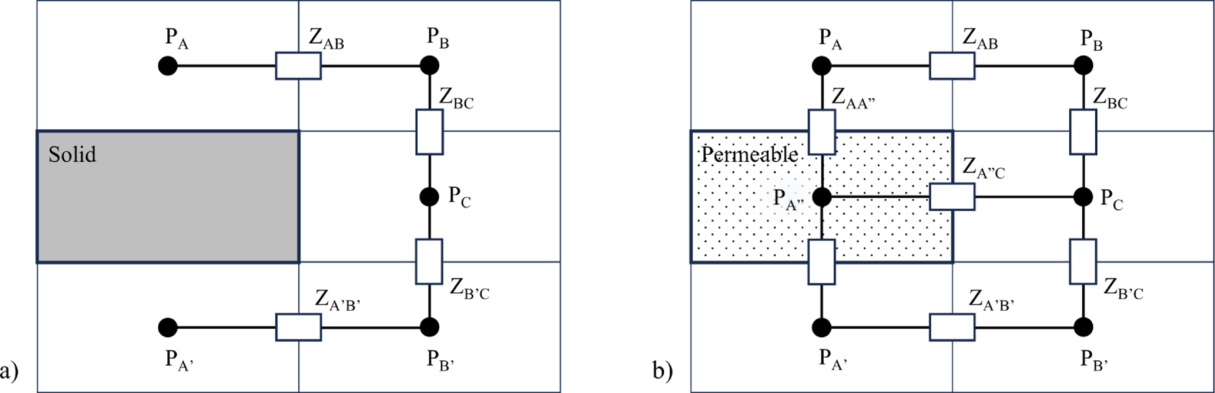
 Z
Z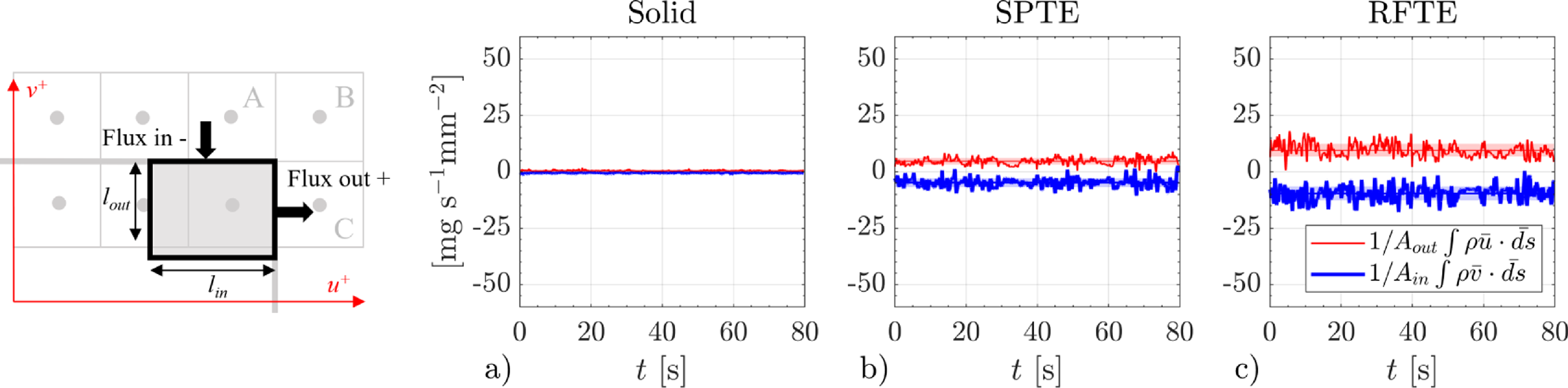
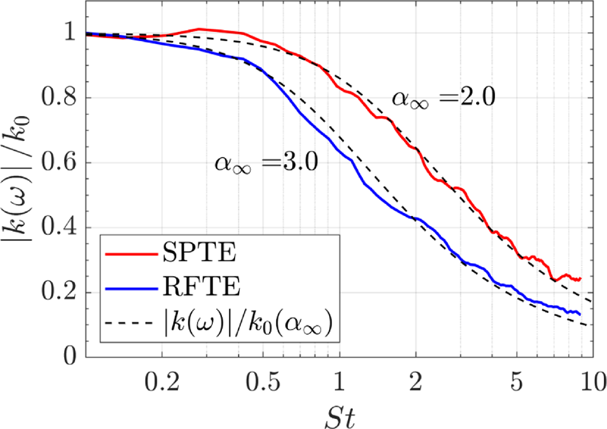
 Λ=
Λ= α∞
α∞


 Open access

