


1. Introduction
Different procedures and parameters are used to understand the formation and evolution of our galaxy. The iron element relative to the hydrogen, [Fe/H], was used for a long time as the main parameter, and still it is used in the new procedures for this purpose. Discovery of the metal-poor stars led the separation of the stars in our galaxy into disc (metal-rich) and halo (metal-poor) populations which occupy the short and large vertical distances of our galaxy, respectively. The need of a third population for fitting the space densities observed by Gilmore & Reid (Reference Gilmore and Reid1983) increased the populations of our galaxy from two to three. The new population covers the stars with intermediate metallicities and vertical distances. Thus, the disc component of our galaxy is separated into two sub-components, thin disc and thick disc. The investigation of the formation and evolution of our galaxy is usually based on these components, thin disc, thick disc, and halo. The ages of the three mentioned galactic components are young, intermediate, and old, in the order just given.
The main source of the iron-peak elements is the Type-Ia supernovae which are produced in a few Gyr. There is another set of elements, alpha ( $\alpha$
) elements, which are mostly produced from the Type II supernovae in about 20 Myr (Wyse & Gilmore Reference Wyse and Gilmore1988). Due to difference between the production times of the iron peak and
$\alpha$
) elements, which are mostly produced from the Type II supernovae in about 20 Myr (Wyse & Gilmore Reference Wyse and Gilmore1988). Due to difference between the production times of the iron peak and $\alpha$
-elements, one expects that old stars are
$\alpha$
-elements, one expects that old stars are $\alpha$
-rich but iron-poor, while the young ones are iron-rich and hence
$\alpha$
-rich but iron-poor, while the young ones are iron-rich and hence $\alpha$
-poor relative to the iron abundance, that is, [
$\alpha$
-poor relative to the iron abundance, that is, [ $\alpha$
/Fe].
$\alpha$
/Fe].
The formation and evolution of our galaxy can be investigated kinematically as well. The procedure used is the combination of the probability function f (U,V,W) and the observed fractions (X) of each population in the solar neighbourhood as explained in Bensby et al. (Reference Bensby, Feltzing and Lundström2003, Reference Bensby, Feltzing, Lundström and Ilyin2005):
 \begin{align}
f(U,V,W) ={} & k\times\exp[-(U_{LSR}^2/2\sigma_{U}^2)\label{eqn1}\end{align}
\begin{align}
f(U,V,W) ={} & k\times\exp[-(U_{LSR}^2/2\sigma_{U}^2)\label{eqn1}\end{align}
 \begin{align} \nonumber
& -((V_{LSR}-V{asym})^2/2\sigma_{V}^2)-(W_{LSR}^2/2\sigma_{W}^2)],
\end{align}
\begin{align} \nonumber
& -((V_{LSR}-V{asym})^2/2\sigma_{V}^2)-(W_{LSR}^2/2\sigma_{W}^2)],
\end{align}
where it is assumed that the galactic space velocity components $U_{LSR}$
,
$U_{LSR}$
, $V_{LSR}$
, and
$V_{LSR}$
, and $W_{LSR}$
of the stellar populations in the thin disc, thick disc, and halo have Gaussian distributions,
$W_{LSR}$
of the stellar populations in the thin disc, thick disc, and halo have Gaussian distributions, $k=[(2\pi)^{3/2}\sigma_U \sigma_V \sigma_W]^{-1}$
normalises the expression,
$k=[(2\pi)^{3/2}\sigma_U \sigma_V \sigma_W]^{-1}$
normalises the expression, $\sigma_U$
,
$\sigma_U$
, $\sigma_V$
, and
$\sigma_V$
, and $\sigma_W$
are the characteristic velocity dispersions, and
$\sigma_W$
are the characteristic velocity dispersions, and $V_{asym}$
is the asymmetric drift. Thus, one gets two relative probabilities for a star as in the following:
$V_{asym}$
is the asymmetric drift. Thus, one gets two relative probabilities for a star as in the following:
 \begin{eqnarray}
TD/D=(X_{TD}/X_D)\times(\,f_{TD}/f_D),\label{eqn2}\end{eqnarray}
\begin{eqnarray}
TD/D=(X_{TD}/X_D)\times(\,f_{TD}/f_D),\label{eqn2}\end{eqnarray}
 \begin{eqnarray} \nonumber
TD/H = (X_{TD}/X_H)\times(\,f_{TD}/f_H),
\end{eqnarray}
\begin{eqnarray} \nonumber
TD/H = (X_{TD}/X_H)\times(\,f_{TD}/f_H),
\end{eqnarray}
where $X_D$
,
$X_D$
, $X_{TD}$
, and
$X_{TD}$
, and $X_H$
refer to the observed local fractions for the thin disc, thick disc, and halo, respectively. If
$X_H$
refer to the observed local fractions for the thin disc, thick disc, and halo, respectively. If $TD/D$
is equal to a big number, the probability of the star in question of being thick-disc star relative to the thin disc is relatively high. For example, in the case of
$TD/D$
is equal to a big number, the probability of the star in question of being thick-disc star relative to the thin disc is relatively high. For example, in the case of $TD/D=10$
, the probability of a star belonging to the thick-disc component is 10 times bigger than the thin disc one. In the opposite case, that is, if
$TD/D=10$
, the probability of a star belonging to the thick-disc component is 10 times bigger than the thin disc one. In the opposite case, that is, if $TD/D$
is a small number, say
$TD/D$
is a small number, say $1/10$
, the star is probably a thin-disc star. A similar case holds for the relative probability
$1/10$
, the star is probably a thin-disc star. A similar case holds for the relative probability $TD/H$
.
$TD/H$
.
The $\alpha$
-elements have been phenomena of galactic research since the beginning of this century. Many studies are based on the distribution of the
$\alpha$
-elements have been phenomena of galactic research since the beginning of this century. Many studies are based on the distribution of the $\alpha$
-elements relative to the iron abundance, [
$\alpha$
-elements relative to the iron abundance, [ $\alpha$
/Fe]
$\alpha$
/Fe] $\,\times\,$
[Fe/H]. Also, the population types of the stars, estimated kinematically, are usually indicated by different symbols on this diagram. One can see the following picture on this diagram: The halo population covers the [Fe/H]-poor and
$\,\times\,$
[Fe/H]. Also, the population types of the stars, estimated kinematically, are usually indicated by different symbols on this diagram. One can see the following picture on this diagram: The halo population covers the [Fe/H]-poor and $\alpha$
-rich stars, and the thick-disc population is dominant with intermediate [Fe/H] and
$\alpha$
-rich stars, and the thick-disc population is dominant with intermediate [Fe/H] and $\alpha$
stars, while the thin-disc stars are [Fe/H]-rich and
$\alpha$
stars, while the thin-disc stars are [Fe/H]-rich and $\alpha$
-poor. These studies can be found in Stephens & Boesgaard (Reference Stephens and Boesgaard2002), Allende Prieto et al. (Reference Allende Prieto, Barklem, Lambert and Cunha2004), Bensby et al. (Reference Bensby, Feltzing and Lundström2003), Bensby et al. (Reference Bensby, Feltzing and Oey2014), Reddy et al. (Reference Reddy, Lambert and Allende Prieto2006), Nissen & Schuster (Reference Nissen and Schuster2010), Adibekyan et al. (Reference Adibekyan, Delgado Mena and Sousa2012), Bovy et al. (Reference Bovy, Rix and Hogg2012), and Haywood et al. (Reference Haywood, DiMatteo, Lehnert, Katz and Gomez2013)and references therein. The largest set of
$\alpha$
-poor. These studies can be found in Stephens & Boesgaard (Reference Stephens and Boesgaard2002), Allende Prieto et al. (Reference Allende Prieto, Barklem, Lambert and Cunha2004), Bensby et al. (Reference Bensby, Feltzing and Lundström2003), Bensby et al. (Reference Bensby, Feltzing and Oey2014), Reddy et al. (Reference Reddy, Lambert and Allende Prieto2006), Nissen & Schuster (Reference Nissen and Schuster2010), Adibekyan et al. (Reference Adibekyan, Delgado Mena and Sousa2012), Bovy et al. (Reference Bovy, Rix and Hogg2012), and Haywood et al. (Reference Haywood, DiMatteo, Lehnert, Katz and Gomez2013)and references therein. The largest set of $\alpha$
-elements is the Hypatia catalogue (Hinkel et al. Reference Hinkel, Timmes, Young, Pagano and Turnbull2014). Alpha abundances can be found also in large surveys, such as the RAdial Velocity Experiment (RAVE) (Steinmetz et al. Reference Steinmetz, Zwitter and Siebert2006), The APO Galactic Evolution Experiment (APOGEE) (Allende Prieto et al. 2008), Sloan Extension for Galactic Understanding and Exploration (SEGUE) (Yanny et al. Reference Yanny, Rockosi and Newberg2009), The Large Sky Area Multi-Object Fibre Spectroscopic Telescope (LAMOST) (Zhao et al. Reference Zhao, Zhao, Chu, Jing and Deng2012), GES (Gilmore et al. Reference Gilmore, Randich and Asplund2012), GALactic Archaeology with HERMES (GALAH) (Heijmans et al. Reference Heijmans, Asplund, Barden, Ian, Suzanne and Hideki2012), and The GIRAFFE Inner Bulge Survey (GIBS) (Zoccali et al. Reference Zoccali, Gonzalez and Vasquez2014).
$\alpha$
-elements is the Hypatia catalogue (Hinkel et al. Reference Hinkel, Timmes, Young, Pagano and Turnbull2014). Alpha abundances can be found also in large surveys, such as the RAdial Velocity Experiment (RAVE) (Steinmetz et al. Reference Steinmetz, Zwitter and Siebert2006), The APO Galactic Evolution Experiment (APOGEE) (Allende Prieto et al. 2008), Sloan Extension for Galactic Understanding and Exploration (SEGUE) (Yanny et al. Reference Yanny, Rockosi and Newberg2009), The Large Sky Area Multi-Object Fibre Spectroscopic Telescope (LAMOST) (Zhao et al. Reference Zhao, Zhao, Chu, Jing and Deng2012), GES (Gilmore et al. Reference Gilmore, Randich and Asplund2012), GALactic Archaeology with HERMES (GALAH) (Heijmans et al. Reference Heijmans, Asplund, Barden, Ian, Suzanne and Hideki2012), and The GIRAFFE Inner Bulge Survey (GIBS) (Zoccali et al. Reference Zoccali, Gonzalez and Vasquez2014).
Although there is a large improvement in attribution of spectroscopic and kinematic data to a given star population, there are still some problems to be solved. For example, Haywood et al. (Reference Haywood, DiMatteo, Lehnert, Katz and Gomez2013) and Hayden et al. (Reference Hayden, Recio-Blanco, de Laverny, Mikolaitis and Worley2017) showed that the metal-rich intermediate stars have kinematics similar to the thin disc. Bland-Hawthorn et al. (Reference Bland-Hawthorn, Sharma and Tepper-Garcia2019) used a different terminology for the two discs of our galaxy, that is, $\alpha$
-rich disc and
$\alpha$
-rich disc and $\alpha$
-poor disc, instead of thick disc and thin disc, respectively. The flaring
$\alpha$
-poor disc, instead of thick disc and thin disc, respectively. The flaring $\alpha$
-poor disc in their Figure 1 indicates a longer scale length for the
$\alpha$
-poor disc in their Figure 1 indicates a longer scale length for the $\alpha$
-poor disc relative to the
$\alpha$
-poor disc relative to the $\alpha$
-rich disc. The simple choice of the boundary between
$\alpha$
-rich disc. The simple choice of the boundary between $\alpha$
-rich disc stars and
$\alpha$
-rich disc stars and $\alpha$
-poor disc stars in the [
$\alpha$
-poor disc stars in the [ $\alpha$
/Fe]
$\alpha$
/Fe] $\,\times\,$
[Fe/H] diagram, in Bland-Hawthorn et al. (Reference Bland-Hawthorn, Sharma and Tepper-Garcia2019), is carried out dynamically where they showed the actions of the two star categories distinct. Another recent work is the study of Buder et al. (Reference Buder, Lind and Ness2019). These authors first showed that stars of the high-
$\,\times\,$
[Fe/H] diagram, in Bland-Hawthorn et al. (Reference Bland-Hawthorn, Sharma and Tepper-Garcia2019), is carried out dynamically where they showed the actions of the two star categories distinct. Another recent work is the study of Buder et al. (Reference Buder, Lind and Ness2019). These authors first showed that stars of the high- $\alpha$
sequence are older (>8 Gyr) than stars in the low-
$\alpha$
sequence are older (>8 Gyr) than stars in the low- $\alpha$
sequence with the iron abundances
$\alpha$
sequence with the iron abundances $-0.7 \lt {\rm [Fe/H]} \lt +0.5$
dex, and then they applied their finding to the metal-rich stars which become indistinguishable in the [
$-0.7 \lt {\rm [Fe/H]} \lt +0.5$
dex, and then they applied their finding to the metal-rich stars which become indistinguishable in the [ $\alpha$
/Fe]
$\alpha$
/Fe] $\,\times\,$
[Fe/H] diagram. Also, Buder et al. (Reference Buder, Lind and Ness2019) found a continuous evolution in the high-
$\,\times\,$
[Fe/H] diagram. Also, Buder et al. (Reference Buder, Lind and Ness2019) found a continuous evolution in the high- $\alpha$
sequence up to super-solar [Fe/H].
$\alpha$
sequence up to super-solar [Fe/H].
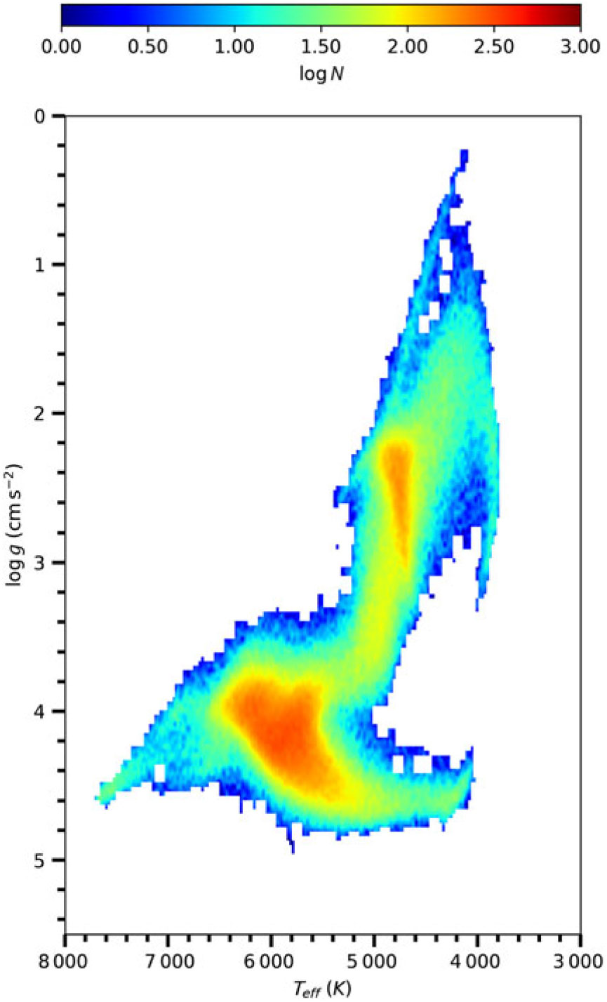
 $\log g \times T_{eff}$
diagram of the stars in the GALAH DR2, colour-coded for the number of stars.
$\log g \times T_{eff}$
diagram of the stars in the GALAH DR2, colour-coded for the number of stars.
The most recent study that we would like to cite is the one of Haywood et al. (Reference Haywood, Snaith, Lehnert, Di Matteo and Khoperskov2019). These authors argue that the galactic disc within 10 kpc has been enriched to solar metallicity by the thick disc. Then, two different enrichments took place: The inner disc, $R \lt 6$
kpc, continued enrichment after a quenching phase (7–10 Gyr), while at larger distances radial flows of gas diluted the metals left by the thick-disc formation. Haywood et al. (Reference Haywood, Snaith, Lehnert, Di Matteo and Khoperskov2019) stated that the strong correlation between ages,
$R \lt 6$
kpc, continued enrichment after a quenching phase (7–10 Gyr), while at larger distances radial flows of gas diluted the metals left by the thick-disc formation. Haywood et al. (Reference Haywood, Snaith, Lehnert, Di Matteo and Khoperskov2019) stated that the strong correlation between ages, $\alpha$
-abundances, and metallicities for the inner disc stars is due to the closed-box-type evolution of the inner disc and bulge. One can see a good fit of the mentioned data to their model. However, the same case does not hold for the outer disc stars, that is, mono-abundance populations are not mono-age populations, because stars with a given age cover a large range in metallicity. As stated by the authors, the birth radius of the stars should be considered to obtain a mono-age population.
$\alpha$
-abundances, and metallicities for the inner disc stars is due to the closed-box-type evolution of the inner disc and bulge. One can see a good fit of the mentioned data to their model. However, the same case does not hold for the outer disc stars, that is, mono-abundance populations are not mono-age populations, because stars with a given age cover a large range in metallicity. As stated by the authors, the birth radius of the stars should be considered to obtain a mono-age population.
The spectroscopic data have the advantage of representing the structure of the gas cloud they were formed, while kinematic data may change by time due to the effect of some structures of our galaxy, such as the central bar, spiral arms, aggregation material, and molecular clouds. On the other hand, it has been shown in the recent studies that there is an overlap between the abundances of metals observed for stars in different populations; that is, the iron metallicity of the old thin-disc stars is compatible with the one of the thick-disc stars (cf. Haywood et al. Reference Haywood, DiMatteo, Lehnert, Katz and Gomez2013). Then, one can deduce that the spectroscopic and kinematic parameters should be combined with age for a better understanding of the formation and evolution of the galactic components, that is, thin disc, thick disc, and halo.
In this study, we used the spectroscopic and astrometric data provided from the GALAH Data Release (DR2) (Buder et al. Reference Buder, Asplund, Duong, Kos, Lind and Ness2018) and Gaia DR2 from the European Space Agency mission Gaia (Gaia Collaboration Reference Collaboration, Prusti and de Bruijne2016, Reference Collaboration, Brown and Vallenari2018), respectively, for a large sample of F- and G-type stars for two purposes: (1) to investigate the distribution of their [ $\alpha$
/Fe] abundances into the thin and thick-disc populations in terms of total space velocity, [Fe/H] abundance, and age and (2) to separate them into two categories such as
$\alpha$
/Fe] abundances into the thin and thick-disc populations in terms of total space velocity, [Fe/H] abundance, and age and (2) to separate them into two categories such as $\alpha$
-rich and
$\alpha$
-rich and $\alpha$
-poor stars with respect to [Fe/H] abundance by using the age parameter, but avoiding any kinematical/dynamical parameter. GALAH is a large-scale stellar spectroscopic survey of our galaxy and designed to deliver chemical information complementary to a large number of stars covered by the Gaia mission. GALAH DR2 (Buder et al. Reference Buder, Asplund, Duong, Kos, Lind and Ness2018) contains 342 682 stars provided with stellar parameters and abundances for up to 23 elements. The High Efficiency and Resolution Multi-Element Spectrograph (HERMES) mounted on the Anglo-Australian Telescope provides multi-object (
$\alpha$
-poor stars with respect to [Fe/H] abundance by using the age parameter, but avoiding any kinematical/dynamical parameter. GALAH is a large-scale stellar spectroscopic survey of our galaxy and designed to deliver chemical information complementary to a large number of stars covered by the Gaia mission. GALAH DR2 (Buder et al. Reference Buder, Asplund, Duong, Kos, Lind and Ness2018) contains 342 682 stars provided with stellar parameters and abundances for up to 23 elements. The High Efficiency and Resolution Multi-Element Spectrograph (HERMES) mounted on the Anglo-Australian Telescope provides multi-object ( $n \approx 392$
) and high resolution (
$n \approx 392$
) and high resolution ( $R\approx 28\,000$
).
$R\approx 28\,000$
).
Gaia relies on the proven principles of ESA’s Hipparcos mission to help solve one of the most difficult yet deeply fundamental challenges in modern astronomy: the creation of an extraordinarily precise three-dimensional map of about one billion stars throughout our galaxy and beyond. The Gaia mission delivers an astronomical catalogue and data archive of unprecedented scope, accuracy, and completeness. Please approve edit to the sentence ‘Combined with the additional…’.Combined with the additional precise astrometric information from the Gaia satellite, one has the ability to determine the precise kinematic, dynamic, and temporal structure of stellar populations throughout the galaxy. We organised the paper as follows. Section 2 is devoted to the star sample, investigation of the sample stars via kinematic, and spectroscopic procedures is given in Section 3, and finally a summary and discussion is presented in Section 4.
2. Star sample
The star sample is provided from the GALAH DR2 survey (Buder et al. Reference Buder, Asplund, Duong, Kos, Lind and Ness2018) which covers the spectral data of 342 682 stars. We applied the following constrains to obtain a star sample of F–G-type dwarf stars with accurate trigonometric parallaxes: 5 250 $\leq T_{eff} \leq$
7 160 K,
$\leq T_{eff} \leq$
7 160 K, $\log g \geq 4$
(cm s-2),
$\log g \geq 4$
(cm s-2), $\sigma_\varpi/\varpi \leq 0.05$
, and
$\sigma_\varpi/\varpi \leq 0.05$
, and $G\leq14$
mag. The 5% trigonometric parallax uncertainties minimise bias. The
$G\leq14$
mag. The 5% trigonometric parallax uncertainties minimise bias. The
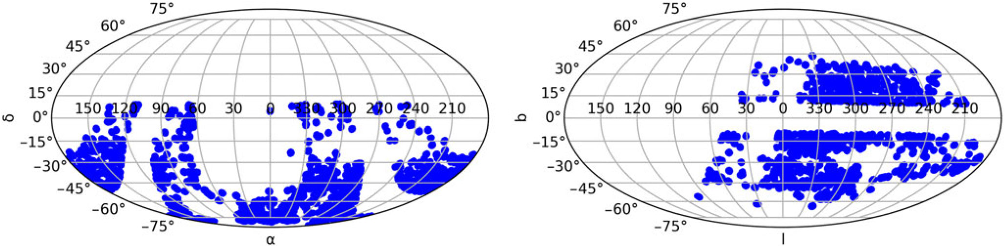
 $\log g \times T_{eff}$
diagram for all stars and the distribution of the 69 157 stars in equatorial and galactic coordinate systems are shown in Figures 1 and 2, respectively. [
$\log g \times T_{eff}$
diagram for all stars and the distribution of the 69 157 stars in equatorial and galactic coordinate systems are shown in Figures 1 and 2, respectively. [ $\alpha/$
Fe] and [Fe/H] abundances as well as the radial velocities are provided from the GALAH DR2 catalogue (Buder et al. Reference Buder, Asplund, Duong, Kos, Lind and Ness2018), while the proper motions and trigonometric parallaxes, used in distance estimations, are taken from the Gaia DR2 (Gaia Collaboration Reference Collaboration, Brown and Vallenari2018). Radial velocities, proper motions, and distances are combined to obtain space velocity components (U, V, W) of the sample stars which are calculated with Johnson & Soderblom (Reference Johnson and Soderblom1987) standard algorithms and transformation matrices of a right-handed system epoch J2000. Hence, U, V, and W are the space velocity components of a star with respect to the Sun, where U is positive towards the galactic centre, V is positive in the direction of the galactic rotation, and W is positive towards the North Galactic Pole. We applied the procedure of Mihalas & Binney (Reference Mihalas, Binney, Ostriker and Spergel1981) to the distribution of the sample stars and estimated the first order of galactic differential rotation corrections for the U and V velocity components. The W velocity component is not affected by galactic differential rotation. The ranges of these corrections are
$\alpha/$
Fe] and [Fe/H] abundances as well as the radial velocities are provided from the GALAH DR2 catalogue (Buder et al. Reference Buder, Asplund, Duong, Kos, Lind and Ness2018), while the proper motions and trigonometric parallaxes, used in distance estimations, are taken from the Gaia DR2 (Gaia Collaboration Reference Collaboration, Brown and Vallenari2018). Radial velocities, proper motions, and distances are combined to obtain space velocity components (U, V, W) of the sample stars which are calculated with Johnson & Soderblom (Reference Johnson and Soderblom1987) standard algorithms and transformation matrices of a right-handed system epoch J2000. Hence, U, V, and W are the space velocity components of a star with respect to the Sun, where U is positive towards the galactic centre, V is positive in the direction of the galactic rotation, and W is positive towards the North Galactic Pole. We applied the procedure of Mihalas & Binney (Reference Mihalas, Binney, Ostriker and Spergel1981) to the distribution of the sample stars and estimated the first order of galactic differential rotation corrections for the U and V velocity components. The W velocity component is not affected by galactic differential rotation. The ranges of these corrections are $-69 \lt dU \lt 29$
and
$-69 \lt dU \lt 29$
and $-4 \lt dV \lt 5$
km s-1 for U and V, respectively, while their means are
$-4 \lt dV \lt 5$
km s-1 for U and V, respectively, while their means are $\langle dU\rangle=-8.53$
and
$\langle dU\rangle=-8.53$
and $\langle dV \rangle=0.43$
km s-1. The galactic rotational velocity of the Sun is adopted as 222.5 km s-1 (Schönrich et al. Reference Schönrich, Binney and Dehnen2010). Then, the space velocity components are reduced by applying the solar local standard of rest (LSR) values of Coşkunoğlu et al. (2011) for all sample stars (U, V, W)
$\langle dV \rangle=0.43$
km s-1. The galactic rotational velocity of the Sun is adopted as 222.5 km s-1 (Schönrich et al. Reference Schönrich, Binney and Dehnen2010). Then, the space velocity components are reduced by applying the solar local standard of rest (LSR) values of Coşkunoğlu et al. (2011) for all sample stars (U, V, W) $_{LSR}$
= (
$_{LSR}$
= ( $8.83\pm0.24$
,
$8.83\pm0.24$
, $14.19\pm0.34$
,
$14.19\pm0.34$
, $6.57\pm0.21$
) km s-1. The numerical values of the characteristic velocity dispersions,
$6.57\pm0.21$
) km s-1. The numerical values of the characteristic velocity dispersions, $\sigma_U$
,
$\sigma_U$
, $\sigma_V$
, and
$\sigma_V$
, and $\sigma_W$
and the asymmetric drift
$\sigma_W$
and the asymmetric drift $V_{asym}$
used in Eq. (1) for our sample stars are provided from Bensby et al. (Reference Bensby, Feltzing and Lundström2003), while the observed local fractions for the thin disc, thick disc, and halo,
$V_{asym}$
used in Eq. (1) for our sample stars are provided from Bensby et al. (Reference Bensby, Feltzing and Lundström2003), while the observed local fractions for the thin disc, thick disc, and halo, $X_D$
,
$X_D$
, $X_{TD}$
, and
$X_{TD}$
, and $X_H$
used in Eq. (2) are taken from Buser et al. (Reference Buser, Rong and Karaali1999), and listed in Table 1.
$X_H$
used in Eq. (2) are taken from Buser et al. (Reference Buser, Rong and Karaali1999), and listed in Table 1.
Distributions of the stars in the GALAH DR2 in the equatorial coordinate (left) and galactic coordinate systems (right).
Numerical values of the characteristic velocity component dispersions, $\sigma_U$
,
$\sigma_U$
, $\sigma_V$
, and
$\sigma_V$
, and $\sigma_W$
, the asymmetric drift
$\sigma_W$
, the asymmetric drift $V_{asym}$
, and the observed local fractions for the thin disc (D), thick disc (TD), and halo (H).
$V_{asym}$
, and the observed local fractions for the thin disc (D), thick disc (TD), and halo (H).
3. Investigation of the sample stars via kinematic and spectroscopic procedures
3.1. Relative probabilities, $[\alpha/{\rm Fe}]$
and
$[{\rm Fe/H}]$
abundances, total space velocities, and ages of the sample stars
$[\alpha/{\rm Fe}]$
and
$[{\rm Fe/H}]$
abundances, total space velocities, and ages of the sample stars


We used the relative probability functions defined in Section 2, $TD/D$
and
$TD/D$
and $TD/H$
, for separation of the sample stars into different populations and determined the
$TD/H$
, for separation of the sample stars into different populations and determined the $[\alpha/{\rm Fe}]$
abundances of the sample stars in each population as well as their
$[\alpha/{\rm Fe}]$
abundances of the sample stars in each population as well as their $S_{LSR}$
total space velocities, [Fe/H] abundances and
$S_{LSR}$
total space velocities, [Fe/H] abundances and $\tau$
ages (Table 2). The reason of using this procedure is that thin-disc stars are
$\tau$
ages (Table 2). The reason of using this procedure is that thin-disc stars are $[\alpha/{\rm Fe}]$
-poor, [Fe/H]-rich, and young and they have relatively small space velocities, while the halo stars are
$[\alpha/{\rm Fe}]$
-poor, [Fe/H]-rich, and young and they have relatively small space velocities, while the halo stars are $[\alpha/{\rm Fe}]$
-rich, [Fe/H]-poor, and old and they have high space velocities; also the numerical values of these parameters for the thick-disc stars are between the numerical values of the two sets of data just mentioned. As noted in Section 2,
$[\alpha/{\rm Fe}]$
-rich, [Fe/H]-poor, and old and they have high space velocities; also the numerical values of these parameters for the thick-disc stars are between the numerical values of the two sets of data just mentioned. As noted in Section 2, $[\alpha/{\rm Fe}]$
and [Fe/H] abundances are provided from GALAH DR2, while the ages of the sample stars are calculated by a procedure given in Önal Taṣ et al. (2018). This procedure is based on Bayesian statistics which includes probability density functions that are obtained from comparative calculations of the theoretical model parameters and the observational parameters (Pont & Eyer Reference Pont and Eyer2004; Jørgensen & Lindegren Reference Jørgensen and Lindegren2005; Duran et al. Reference Duran, Ak and Bilir2013). Following the literature, we separated the sample stars into four populations, that is, high-probability thin disc:
$[\alpha/{\rm Fe}]$
and [Fe/H] abundances are provided from GALAH DR2, while the ages of the sample stars are calculated by a procedure given in Önal Taṣ et al. (2018). This procedure is based on Bayesian statistics which includes probability density functions that are obtained from comparative calculations of the theoretical model parameters and the observational parameters (Pont & Eyer Reference Pont and Eyer2004; Jørgensen & Lindegren Reference Jørgensen and Lindegren2005; Duran et al. Reference Duran, Ak and Bilir2013). Following the literature, we separated the sample stars into four populations, that is, high-probability thin disc: $TD/D\leq 0.1$
, low-probability thin disc:
$TD/D\leq 0.1$
, low-probability thin disc: $0.1 \lt TD/D\leq 1$
, low-probability thick disc:
$0.1 \lt TD/D\leq 1$
, low-probability thick disc: $1 \lt TD/D\leq 10$
, and high-probability thick disc:
$1 \lt TD/D\leq 10$
, and high-probability thick disc: $TD/D>10$
. The GALAH probes mainly the thin and thick discs of the galaxy. Hence, we assume that our sample (statistically) does not cover any halo star. Stars with
$TD/D>10$
. The GALAH probes mainly the thin and thick discs of the galaxy. Hence, we assume that our sample (statistically) does not cover any halo star. Stars with $0.1 \lt TD/D\leq 10$
are also called ‘in-between stars’ (Bensby et al. Reference Bensby, Feltzing, Lundström and Ilyin2005) or ‘transit stars between D and TD’ in the literature (Adibekyan et al. Reference Adibekyan, Delgado Mena and Sousa2012).
$0.1 \lt TD/D\leq 10$
are also called ‘in-between stars’ (Bensby et al. Reference Bensby, Feltzing, Lundström and Ilyin2005) or ‘transit stars between D and TD’ in the literature (Adibekyan et al. Reference Adibekyan, Delgado Mena and Sousa2012).
Data for sample stars. The columns give ID, star, total space velocity, relative population probabilities of the stars, $[\alpha/{\rm Fe}]$
and [Fe/H] abundances, and age.
$[\alpha/{\rm Fe}]$
and [Fe/H] abundances, and age.
We plotted the [ $\alpha/$
Fe] abundances against
$\alpha/$
Fe] abundances against $S_{LSR}$
in three panels of Figure 3, colour-coded for the number of stars (a), colour-coded for the relative probability
$S_{LSR}$
in three panels of Figure 3, colour-coded for the number of stars (a), colour-coded for the relative probability $TD/D$
(b), and colour-coded for the age
$TD/D$
(b), and colour-coded for the age $\tau$
(c), for a first approximation of the distribution of the sample stars into different sub-samples defined by the parameters just mentioned. Panel (a) shows that the sample stars are dominant in the total space velocity interval of
$\tau$
(c), for a first approximation of the distribution of the sample stars into different sub-samples defined by the parameters just mentioned. Panel (a) shows that the sample stars are dominant in the total space velocity interval of $S_{LSR}\,{\lt}\,100$
km s-1, while one can see a limited number of stars with total velocity as high as
$S_{LSR}\,{\lt}\,100$
km s-1, while one can see a limited number of stars with total velocity as high as $S_{LSR}\approx 175$
km s-1. From the other hand, one can deduce from the same panel that most of the sample stars lie in the interval
$S_{LSR}\approx 175$
km s-1. From the other hand, one can deduce from the same panel that most of the sample stars lie in the interval $-0.10 \lt [\alpha/{\rm Fe}]\leq 0.15$
dex, and as the stars with
$-0.10 \lt [\alpha/{\rm Fe}]\leq 0.15$
dex, and as the stars with $[\alpha/{\rm Fe}]>0.15$
dex are relatively small in number, we can say that our sample stars are
$[\alpha/{\rm Fe}]>0.15$
dex are relatively small in number, we can say that our sample stars are $\alpha$
-poor ones. Another result that can be deduced from this panel is that the
$\alpha$
-poor ones. Another result that can be deduced from this panel is that the $[\alpha/{\rm Fe}]$
abundances of the stars with the same total space velocity may be different; one can be
$[\alpha/{\rm Fe}]$
abundances of the stars with the same total space velocity may be different; one can be $\alpha$
-poor, while another one may be relatively a rich star, for example.
$\alpha$
-poor, while another one may be relatively a rich star, for example.
Distribution of the $[\alpha/{\rm Fe}]$
abundances against the total space velocities (
$[\alpha/{\rm Fe}]$
abundances against the total space velocities ( $S_{LSR}$
) in three panels: (a) colour-coded for the number of stars, (b) colour-coded for the relative probability (
$S_{LSR}$
) in three panels: (a) colour-coded for the number of stars, (b) colour-coded for the relative probability ( $TD/D$
), and (c) colour-coded for the age (
$TD/D$
), and (c) colour-coded for the age ( $\tau$
).
$\tau$
).
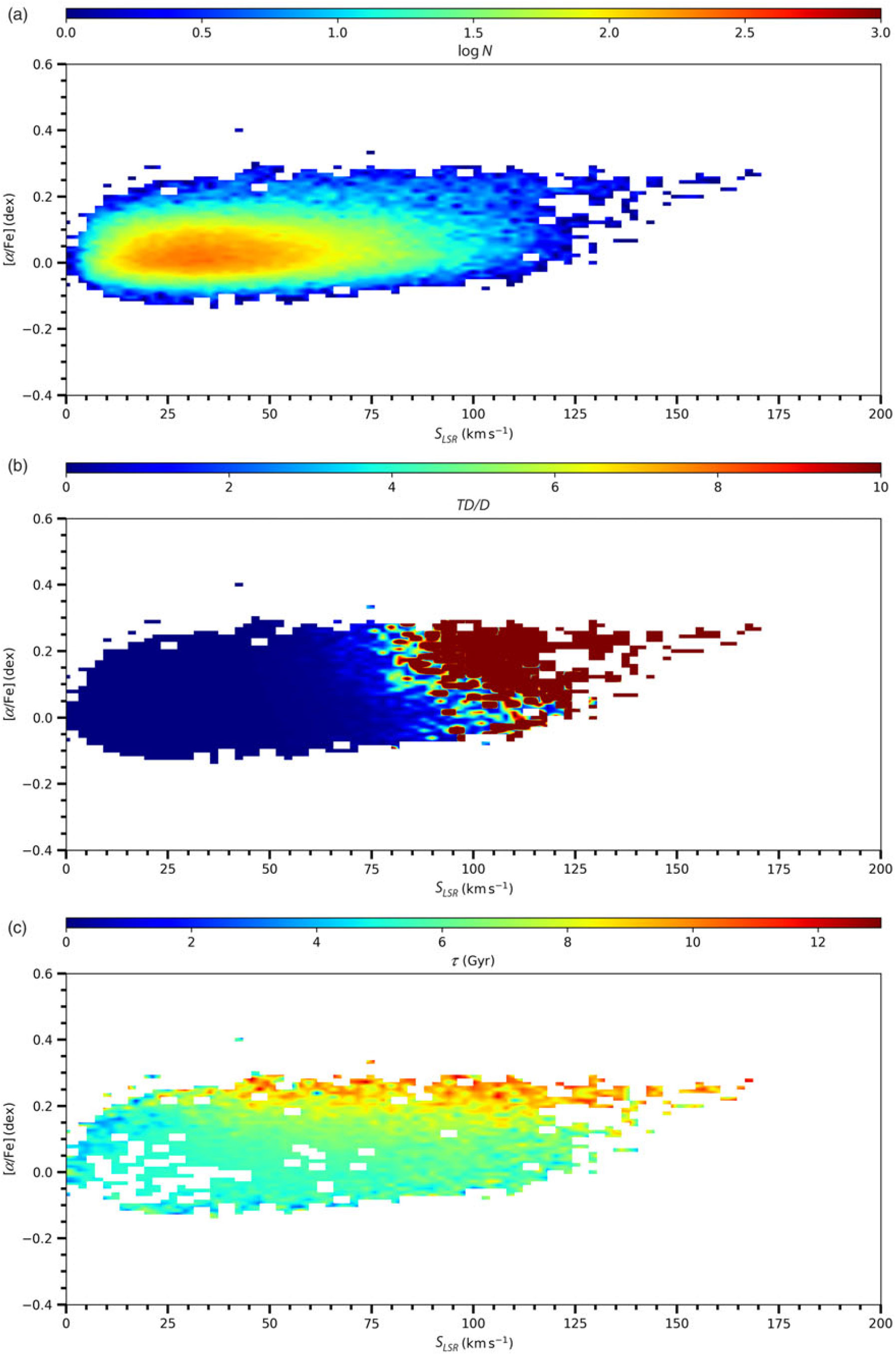
Panel (b) of the same figure shows that the $TD/D$
relative probabilities of the stars with relatively high total space velocities,
$TD/D$
relative probabilities of the stars with relatively high total space velocities, $S_{LSR}>80$
km s-1, are relatively high, while the
$S_{LSR}>80$
km s-1, are relatively high, while the $TD/D$
relative probabilities of the stars with lower total space velocities,
$TD/D$
relative probabilities of the stars with lower total space velocities, $S_{LSR} \lt 80$
km s-1, are relatively low. Stars in the second category are also dominant in this panel, which indicates that the thin-disc stars are dominant relative to the thick-disc stars, in our sample.
$S_{LSR} \lt 80$
km s-1, are relatively low. Stars in the second category are also dominant in this panel, which indicates that the thin-disc stars are dominant relative to the thick-disc stars, in our sample.
In Panel (c), the $\alpha$
-abundances of the stars older than 8 Gyr are higher than the ones of younger stars, that is,
$\alpha$
-abundances of the stars older than 8 Gyr are higher than the ones of younger stars, that is, $[\alpha/{\rm Fe}]> 0.15$
dex for stars with total space velocities
$[\alpha/{\rm Fe}]> 0.15$
dex for stars with total space velocities $S_{LSR}>50$
km s–1 and
$S_{LSR}>50$
km s–1 and $[\alpha/{\rm Fe}]>0.2$
dex for stars with
$[\alpha/{\rm Fe}]>0.2$
dex for stars with $25 \lt S_{LSR} \lt 50$
km s–1. We should emphasise that although the
$25 \lt S_{LSR} \lt 50$
km s–1. We should emphasise that although the $[\alpha/{\rm Fe}]$
abundances of a group of stars with
$[\alpha/{\rm Fe}]$
abundances of a group of stars with $S \lt 25$
km s–1 are relatively high,
$S \lt 25$
km s–1 are relatively high, $[\alpha/{\rm Fe}]>0.15$
dex, their ages are less than 8 Gyr.
$[\alpha/{\rm Fe}]>0.15$
dex, their ages are less than 8 Gyr.
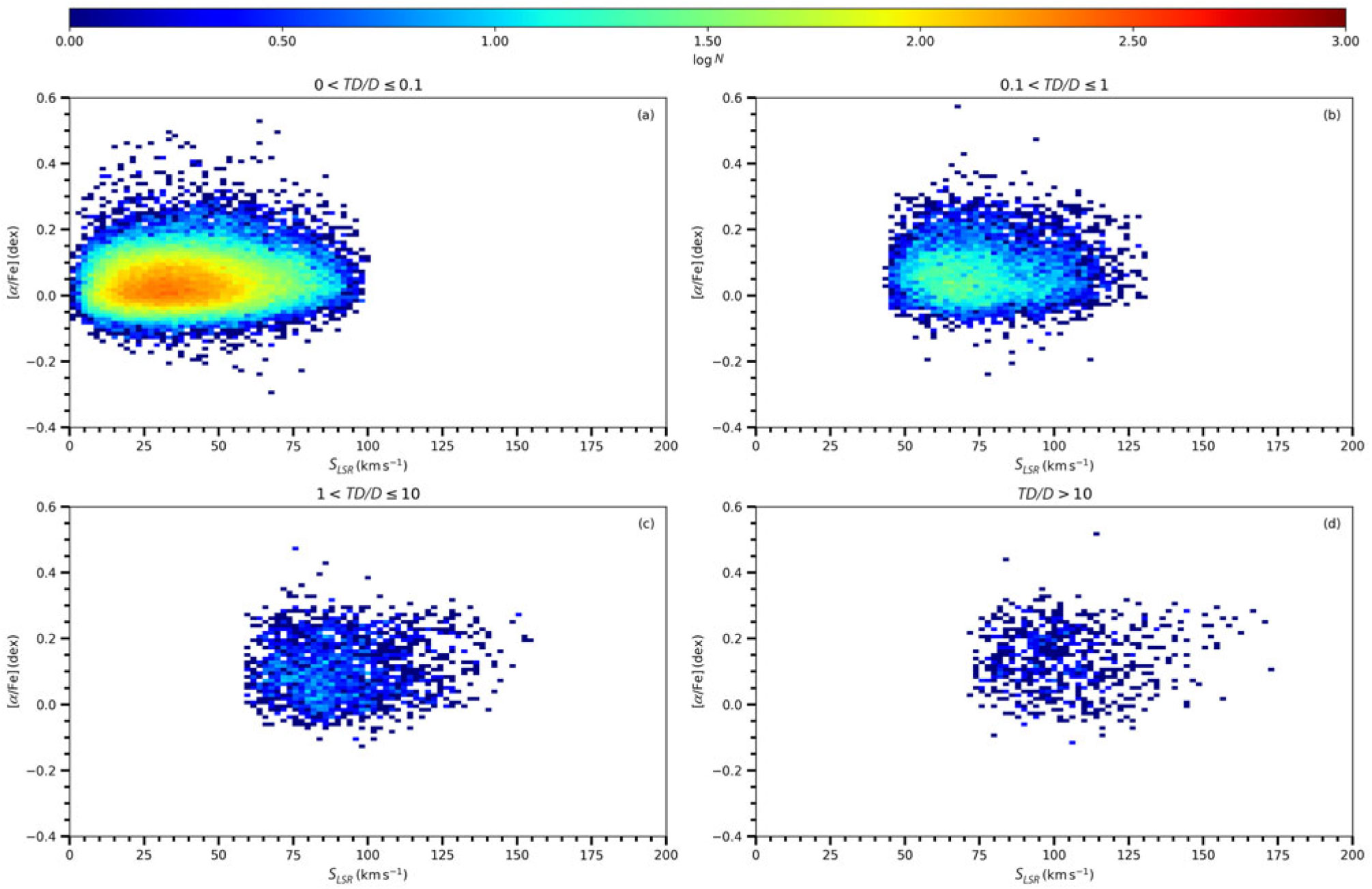
We plotted the $[\alpha/{\rm Fe}]$
abundances versus
$[\alpha/{\rm Fe}]$
abundances versus $S_{LSR}$
velocities for each relative probability function,
$S_{LSR}$
velocities for each relative probability function, $0 \lt TD/D\leq 0.1$
,
$0 \lt TD/D\leq 0.1$
, $0.1 \lt TD/D \leq 1$
,
$0.1 \lt TD/D \leq 1$
, $1 \lt TD/D \leq 10$
, and
$1 \lt TD/D \leq 10$
, and $TD/D>10$
in Figure 4 for a comprehensive investigation of the total space velocity of the sample stars in our study. Figure 4 shows that the number of stars with relative probability
$TD/D>10$
in Figure 4 for a comprehensive investigation of the total space velocity of the sample stars in our study. Figure 4 shows that the number of stars with relative probability $0 \lt TD/D\leq0.1$
in Panel (a) is maximum, while they decrease gradually when one goes to Panels (b)–(d), which cover the stars with relative probabilities,
$0 \lt TD/D\leq0.1$
in Panel (a) is maximum, while they decrease gradually when one goes to Panels (b)–(d), which cover the stars with relative probabilities, $0.1 \lt TD/D \leq 1$
,
$0.1 \lt TD/D \leq 1$
, $1 \lt TD/D \leq 10$
, and
$1 \lt TD/D \leq 10$
, and $TD/D>10$
, respectively. All stars with
$TD/D>10$
, respectively. All stars with $S_{LSR} \lt 45$
km s–1 lie in Panel (a) and they have relative probabilities
$S_{LSR} \lt 45$
km s–1 lie in Panel (a) and they have relative probabilities $0 \lt TD/D \leq 0.1$
. The lower and upper limits of the
$0 \lt TD/D \leq 0.1$
. The lower and upper limits of the $S_{LSR}$
velocity in panels (a)–(d) increase gradually. However, there is overlapping between the
$S_{LSR}$
velocity in panels (a)–(d) increase gradually. However, there is overlapping between the $S_{LSR}$
velocities of the stars in any two panels, including Panels (a) and (d). That is, stars cannot be separated to the thin-disc and thick-disc populations by using only their total space velocities.
$S_{LSR}$
velocities of the stars in any two panels, including Panels (a) and (d). That is, stars cannot be separated to the thin-disc and thick-disc populations by using only their total space velocities.
Distributions of the $[\alpha/{\rm Fe}]$
abundances against the total space velocities (
$[\alpha/{\rm Fe}]$
abundances against the total space velocities ( $S_{LSR}$
) for four relative probability functions:
$S_{LSR}$
) for four relative probability functions: $0 \lt TD/D\leq 0.1$
,
$0 \lt TD/D\leq 0.1$
, $0.1 \lt TD/D\leq 1$
,
$0.1 \lt TD/D\leq 1$
, $1 \lt TD/D\leq 10$
, and
$1 \lt TD/D\leq 10$
, and $TD/D>10$
.
$TD/D>10$
.
The total space velocities, ages, and number of the sample stars are also investigated in seven sub-sets of the $[\alpha/{\rm Fe}]$
abundance that is,
$[\alpha/{\rm Fe}]$
abundance that is, $[\alpha/{\rm Fe}]\leq -0.2$
,
$[\alpha/{\rm Fe}]\leq -0.2$
, $-0.2 \lt [\alpha/{\rm Fe}]\leq 0$
,
$-0.2 \lt [\alpha/{\rm Fe}]\leq 0$
, $0 \lt [\alpha/{\rm Fe}]\leq 0.1$
,
$0 \lt [\alpha/{\rm Fe}]\leq 0.1$
, $0.1 \lt [\alpha/{\rm Fe}]\leq 0.2$
,
$0.1 \lt [\alpha/{\rm Fe}]\leq 0.2$
, $0.2 \lt [\alpha/{\rm Fe}]\leq 0.3$
,
$0.2 \lt [\alpha/{\rm Fe}]\leq 0.3$
, $0.3 \lt [\alpha/{\rm Fe}]\leq 0.4$
, and
$0.3 \lt [\alpha/{\rm Fe}]\leq 0.4$
, and $0.4 \lt [\alpha/{\rm Fe}]\leq 0.7$
dex. We omitted discussion of the stars with
$0.4 \lt [\alpha/{\rm Fe}]\leq 0.7$
dex. We omitted discussion of the stars with $[\alpha/{\rm Fe}]\leq -0.2$
dex due to less number of stars, nine stars. Table 3 shows that in all sub-intervals of
$[\alpha/{\rm Fe}]\leq -0.2$
dex due to less number of stars, nine stars. Table 3 shows that in all sub-intervals of $[\alpha/{\rm Fe}]$
, the total space velocity interval of the high-probability thin-disc stars (
$[\alpha/{\rm Fe}]$
, the total space velocity interval of the high-probability thin-disc stars ( $0 \lt TD/D \leq 0.1$
) is limited with
$0 \lt TD/D \leq 0.1$
) is limited with $0 \lt S_{LSR}\leq 100$
km s–1, while its lower and upper limits shift gradually to higher values when one goes to low-probability thin-disc (
$0 \lt S_{LSR}\leq 100$
km s–1, while its lower and upper limits shift gradually to higher values when one goes to low-probability thin-disc ( $0.1 \lt TD/D \leq 1$
), low-probability thick-disc (
$0.1 \lt TD/D \leq 1$
), low-probability thick-disc ( $1 \lt TD/D\leq 10$
), and high-probability thick-disc (
$1 \lt TD/D\leq 10$
), and high-probability thick-disc ( $TD/D>10$
) stars. Also, the number of high-probability thin-disc stars is maximum in all
$TD/D>10$
) stars. Also, the number of high-probability thin-disc stars is maximum in all $[\alpha/{\rm Fe}]$
sub-intervals. This is interesting, because one expects the number of high-probability thick-disc stars to dominate in the high
$[\alpha/{\rm Fe}]$
sub-intervals. This is interesting, because one expects the number of high-probability thick-disc stars to dominate in the high $[\alpha/{\rm Fe}]$
-intervals. However, we should emphasise that the percentage of the high-probability thick-disc stars is rather higher in two high
$[\alpha/{\rm Fe}]$
-intervals. However, we should emphasise that the percentage of the high-probability thick-disc stars is rather higher in two high $[\alpha/{\rm Fe}]$
-intervals, that is, 28.4
$[\alpha/{\rm Fe}]$
-intervals, that is, 28.4 $\%$
and 26.6
$\%$
and 26.6 $\%$
in the sub-intervals
$\%$
in the sub-intervals $0.2 \lt [\alpha/{\rm Fe}]\leq 0.3$
and
$0.2 \lt [\alpha/{\rm Fe}]\leq 0.3$
and $0.3 \lt [\alpha/{\rm Fe}]\leq 0.4$
dex, respectively. Another interesting result is that high-probability thin-disc stars are dominant in the high abundance (
$0.3 \lt [\alpha/{\rm Fe}]\leq 0.4$
dex, respectively. Another interesting result is that high-probability thin-disc stars are dominant in the high abundance ( $0.4 \lt [\alpha/{\rm Fe}]\leq 0.7$
dex). Their total space velocities are relatively small,
$0.4 \lt [\alpha/{\rm Fe}]\leq 0.7$
dex). Their total space velocities are relatively small, $20.21\leq S_{LSR} \leq 61.32$
km s–1, and they are relatively young stars,
$20.21\leq S_{LSR} \leq 61.32$
km s–1, and they are relatively young stars, $3.71 \leq \tau \leq 7.60$
Gyr. However, this unexpected finding cannot be generalised for the distribution of the
$3.71 \leq \tau \leq 7.60$
Gyr. However, this unexpected finding cannot be generalised for the distribution of the $[\alpha/{\rm Fe}]$
abundances into different populations, but it should be a result of selection effect of the sample stars (see Section 4 for detail).
$[\alpha/{\rm Fe}]$
abundances into different populations, but it should be a result of selection effect of the sample stars (see Section 4 for detail).
The total space velocities and ages of stars in seven $[\alpha/{\rm Fe}]$
sub-intervals:
$[\alpha/{\rm Fe}]$
sub-intervals: $[\alpha/{\rm Fe}]\leq -0.2$
,
$[\alpha/{\rm Fe}]\leq -0.2$
, $-0.2 \lt [\alpha/{\rm Fe}]\leq 0$
,
$-0.2 \lt [\alpha/{\rm Fe}]\leq 0$
, $0 \lt [\alpha/{\rm Fe}]\leq 0.1$
,
$0 \lt [\alpha/{\rm Fe}]\leq 0.1$
, $0.1 \lt [\alpha/{\rm Fe}]\leq 0.2$
,
$0.1 \lt [\alpha/{\rm Fe}]\leq 0.2$
, $0.2 \lt [\alpha/{\rm Fe}]\leq 0.3$
,
$0.2 \lt [\alpha/{\rm Fe}]\leq 0.3$
, $0.3 \lt [\alpha/{\rm Fe}]\leq 0.4$
, and
$0.3 \lt [\alpha/{\rm Fe}]\leq 0.4$
, and $0.4 \lt [\alpha/{\rm Fe}]\leq 0.7$
dex in terms of four relative probability intervals defined in the text. The total number of stars in the cited sub-intervals are 9, 17 027, 39 508, 10 312, 2 091, 169, and 41, respectively.
$0.4 \lt [\alpha/{\rm Fe}]\leq 0.7$
dex in terms of four relative probability intervals defined in the text. The total number of stars in the cited sub-intervals are 9, 17 027, 39 508, 10 312, 2 091, 169, and 41, respectively.
Table 3 shows that relatively young stars are dominant in the high-probability thin-disc population ( $0 \lt TD/D \leq 0.1$
). However, there are also stars as old as
$0 \lt TD/D \leq 0.1$
). However, there are also stars as old as $\tau= 11.15$
Gyr in other populations. The general trend of the age for our sample stars is in agreement with the cited one in the literature; that is, it increases with increasing of the
$\tau= 11.15$
Gyr in other populations. The general trend of the age for our sample stars is in agreement with the cited one in the literature; that is, it increases with increasing of the $[\alpha/{\rm Fe}]$
abundance as well as with total space velocity, and with the four populations in the order of high-probability thin disc, low-probability thin disc, low-probability thick disc, and high-probability thick disc. The distributions of the sample stars in number into the relative probability functions are as follows:
$[\alpha/{\rm Fe}]$
abundance as well as with total space velocity, and with the four populations in the order of high-probability thin disc, low-probability thin disc, low-probability thick disc, and high-probability thick disc. The distributions of the sample stars in number into the relative probability functions are as follows: $0 \lt TD/D \leq 0.1$
: 58 646 (84.8
$0 \lt TD/D \leq 0.1$
: 58 646 (84.8 $\%$
),
$\%$
), $0.1 \lt TD/D \leq 1$
: 7 077 (10.2
$0.1 \lt TD/D \leq 1$
: 7 077 (10.2 $\%$
),
$\%$
), $1 \lt TD/D \leq 10$
: 1 990 (2.9
$1 \lt TD/D \leq 10$
: 1 990 (2.9 $\%$
),
$\%$
), $TD/D>10$
: 1 435 (2.1
$TD/D>10$
: 1 435 (2.1 $\%$
), and nine stars with
$\%$
), and nine stars with $0 \lt TD/D \leq 1$
which are led out of discussion.
$0 \lt TD/D \leq 1$
which are led out of discussion.
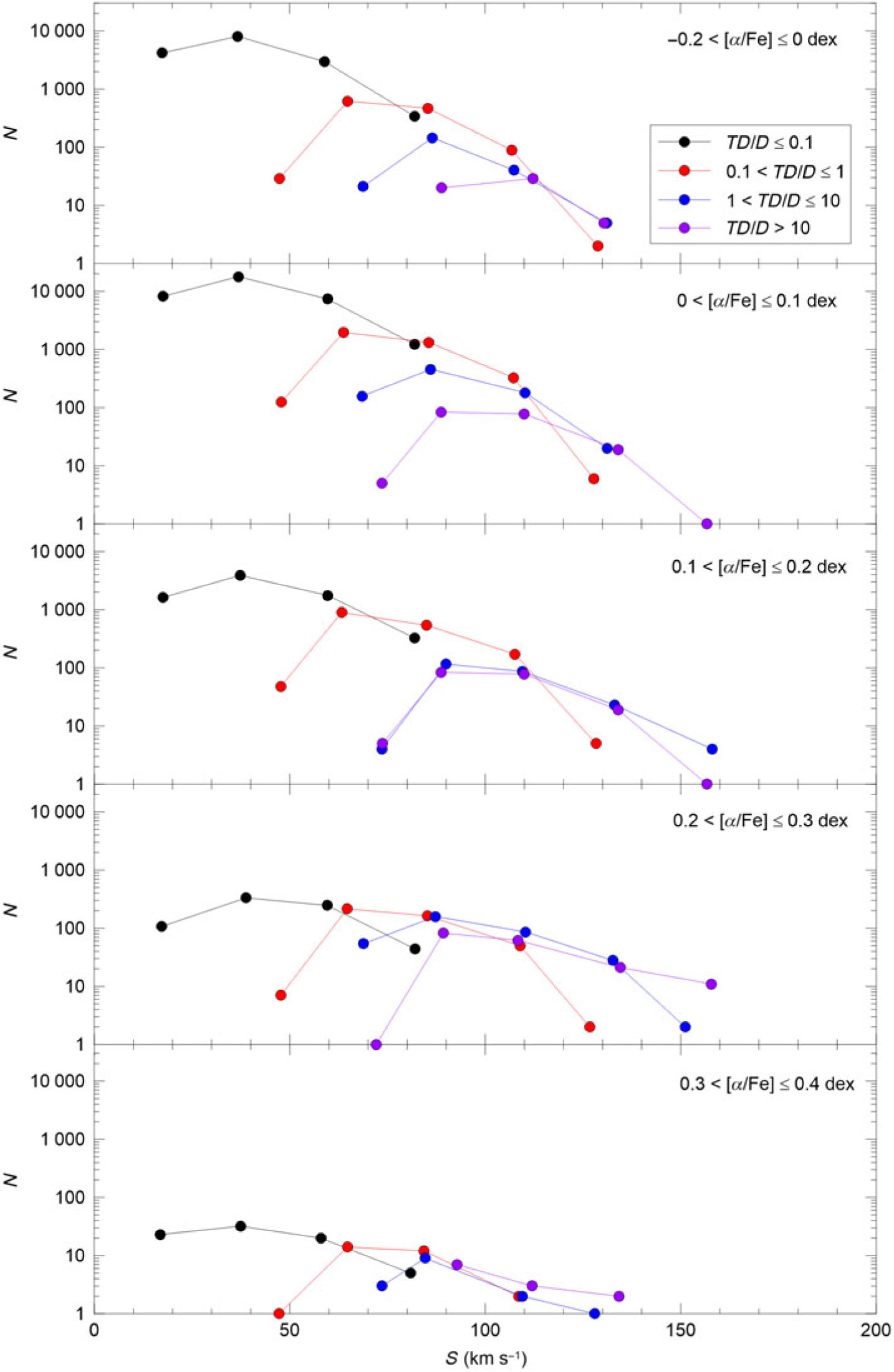
We plotted the frequency polygons of the total space velocities to investigate their trend for each relative probability function of five sub-intervals of $[\alpha/{\rm Fe}]$
where sufficient number of stars are present for discussion, that is,
$[\alpha/{\rm Fe}]$
where sufficient number of stars are present for discussion, that is, $-0.2 \lt [\alpha/{\rm Fe}]\leq 0$
,
$-0.2 \lt [\alpha/{\rm Fe}]\leq 0$
, $0 \lt [\alpha/{\rm Fe}]\leq 0.1$
,
$0 \lt [\alpha/{\rm Fe}]\leq 0.1$
, $0.1 \lt [\alpha/{\rm Fe}]\leq 0.2$
,
$0.1 \lt [\alpha/{\rm Fe}]\leq 0.2$
, $0.2 \lt [\alpha/{\rm Fe}]\leq 0.3$
, and
$0.2 \lt [\alpha/{\rm Fe}]\leq 0.3$
, and $0.3 \lt [\alpha/{\rm Fe}]\leq 0.4$
dex. Figure 5 confirms the results just cited; that is, the number of high-probability thin disc stars (
$0.3 \lt [\alpha/{\rm Fe}]\leq 0.4$
dex. Figure 5 confirms the results just cited; that is, the number of high-probability thin disc stars ( $0 \lt TD/D\leq 0.1$
) is maximum in all sub-intervals of
$0 \lt TD/D\leq 0.1$
) is maximum in all sub-intervals of $[\alpha/{\rm Fe}]$
, the lower limit of the total space velocity shifts to larger values as a function of the relative probability
$[\alpha/{\rm Fe}]$
, the lower limit of the total space velocity shifts to larger values as a function of the relative probability $TD/D$
, and there is overlapping between the total space velocities of the stars with different relative probabilities, including
$TD/D$
, and there is overlapping between the total space velocities of the stars with different relative probabilities, including $0 \lt TD/D\leq 0.1$
and
$0 \lt TD/D\leq 0.1$
and $TD/D>10$
which correspond to the high-probability thin disc and high-probability thick disc, respectively. Then, here again, we can deduce that the total space velocity of a star is not a sufficient parameter to assign its population type.
$TD/D>10$
which correspond to the high-probability thin disc and high-probability thick disc, respectively. Then, here again, we can deduce that the total space velocity of a star is not a sufficient parameter to assign its population type.
The frequency polygons of the total space velocity ( $S_{LSR}$
) for four relative probability functions,
$S_{LSR}$
) for four relative probability functions, $0 \lt TD/D\leq 0.1$
,
$0 \lt TD/D\leq 0.1$
, $0.1 \lt TD/D\leq 1$
,
$0.1 \lt TD/D\leq 1$
, $1 \lt TD/D\leq 10$
, and
$1 \lt TD/D\leq 10$
, and $TD/D>10$
, for five sub-intervals of
$TD/D>10$
, for five sub-intervals of $[\alpha /{\rm Fe}]$
as indicated in five panels of this figure.
$[\alpha /{\rm Fe}]$
as indicated in five panels of this figure.
We investigated the distributions for the [Fe/H] abundances and ages ( $\tau$
) of the sample stars for four populations defined by the relative probabilities
$\tau$
) of the sample stars for four populations defined by the relative probabilities $TD/D\leq0.1$
,
$TD/D\leq0.1$
, $0.1 \lt TD/D \leq1$
,
$0.1 \lt TD/D \leq1$
, $1 \lt TD/D\leq 10$
, and
$1 \lt TD/D\leq 10$
, and $TD/D>10$
without taking into account the
$TD/D>10$
without taking into account the $[\alpha/{\rm Fe}]$
abundance of the stars. Table 4 shows that the range of the [Fe/H] abundance is rather large,
$[\alpha/{\rm Fe}]$
abundance of the stars. Table 4 shows that the range of the [Fe/H] abundance is rather large, $-1.3 \lt {\rm [Fe/H]}\leq 0.6$
dex. However, the number of [Fe/H]-poor stars is relatively small. Hence, we considered only the stars with
$-1.3 \lt {\rm [Fe/H]}\leq 0.6$
dex. However, the number of [Fe/H]-poor stars is relatively small. Hence, we considered only the stars with $\langle{\rm [Fe/H]}\rangle\pm 2\sigma$
, where
$\langle{\rm [Fe/H]}\rangle\pm 2\sigma$
, where $\sigma$
is the standard deviation of (all) stars in each population. This constraint limits the range of the [Fe/H] abundance for the populations, in the order just cited, as follows: (–0.6, 0.4], (–0.7, 0.4], (–0.8, 0.4], and (–1.0, 0.2]. The numbers of stars so defined are in boldface in the table. Then, one can say that the lower limit of the range shifts to the poor [Fe/H] abundance values gradually when one goes from the high-probability thin disc to the high-probability thick disc. The same trend holds for the mean of the [Fe/H] abundance estimated for all stars in a population, that is, –0.08, –0.12, –0.19, and –0.37 dex. The most interesting thing in this table is the existence of an unexpected number of [Fe/H]-poor high-probability thin-disc stars, that is, 1 859 stars with
$\sigma$
is the standard deviation of (all) stars in each population. This constraint limits the range of the [Fe/H] abundance for the populations, in the order just cited, as follows: (–0.6, 0.4], (–0.7, 0.4], (–0.8, 0.4], and (–1.0, 0.2]. The numbers of stars so defined are in boldface in the table. Then, one can say that the lower limit of the range shifts to the poor [Fe/H] abundance values gradually when one goes from the high-probability thin disc to the high-probability thick disc. The same trend holds for the mean of the [Fe/H] abundance estimated for all stars in a population, that is, –0.08, –0.12, –0.19, and –0.37 dex. The most interesting thing in this table is the existence of an unexpected number of [Fe/H]-poor high-probability thin-disc stars, that is, 1 859 stars with ${\rm[Fe/H]} \lt -0.5$
dex.
${\rm[Fe/H]} \lt -0.5$
dex.
Frequency distribution for the [Fe/H] abundance of the sample stars in four relative probability intervals. N indicates the number of stars. The total number of stars is 69 157. Figures with bold face are explained in the text.
The ages of 75 stars could not be estimated, hence the number of the star sample reduced to 69 082. The ranges for the age of the stars in four populations are rather large (Table 5), that is, (0, 13], (1, 13], (1.5, 13], and (1.5, 13] for $TD/D \leq 0.1$
,
$TD/D \leq 0.1$
, $0.1 \lt TD/D \leq 1$
,
$0.1 \lt TD/D \leq 1$
, $1 \lt TD/D \leq 10$
, and
$1 \lt TD/D \leq 10$
, and $TD/D>10$
, respectively. However, they reduce as follows when one considers the data for
$TD/D>10$
, respectively. However, they reduce as follows when one considers the data for $\langle\tau\rangle \pm2\sigma$
: high-probability thin disc:
$\langle\tau\rangle \pm2\sigma$
: high-probability thin disc: $2 \lt \tau \leq 9$
Gyr, low-probability thin disc:
$2 \lt \tau \leq 9$
Gyr, low-probability thin disc: $2.5 \lt \tau \leq 10$
Gyr, low-probability thick disc:
$2.5 \lt \tau \leq 10$
Gyr, low-probability thick disc: $3 \lt \tau \leq 11$
Gyr, and high-probability thick disc:
$3 \lt \tau \leq 11$
Gyr, and high-probability thick disc: $3.5 \lt \tau \leq 12.5$
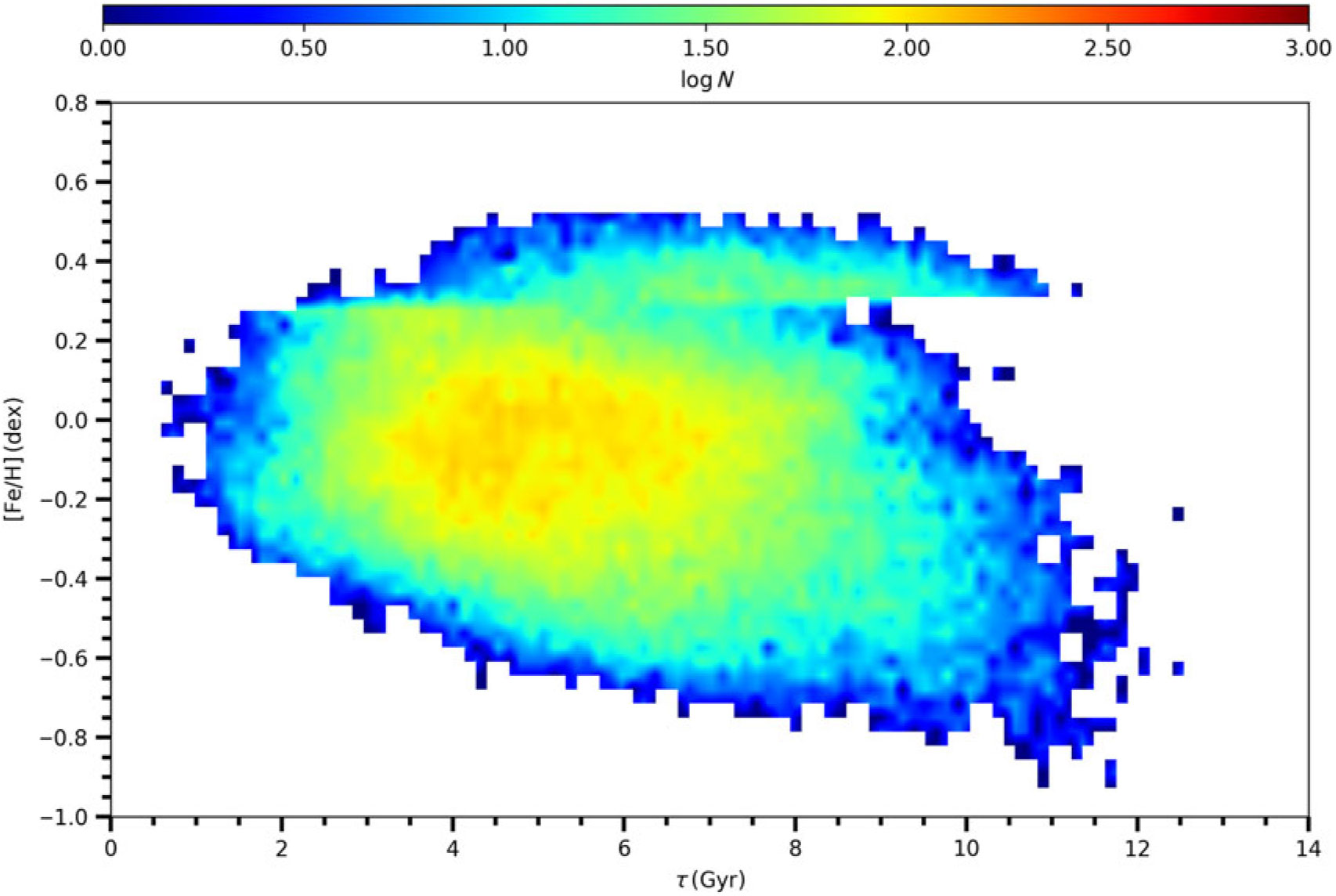
Gyr. The numbers of stars so defined are in boldface in the table. The most interesting thing in this table is the existence of 2 290 high-probability thin-disc stars older than 9 Gyr where about two dozen of them are coeval with the Universe. Figure 6 shows that the [Fe/H] poor stars, that is,
$3.5 \lt \tau \leq 12.5$
Gyr. The numbers of stars so defined are in boldface in the table. The most interesting thing in this table is the existence of 2 290 high-probability thin-disc stars older than 9 Gyr where about two dozen of them are coeval with the Universe. Figure 6 shows that the [Fe/H] poor stars, that is, ${\rm [Fe/H]} \lt -0.5$
dex, are dominant by the old stars. Hence, one can say that most of the stars with unexpected [Fe/H] abundances (the 1 859 stars mentioned in the foregoing paragraph) and 2 290 stars just mentioned, are identical (we shall discuss this problem in Section 4).
${\rm [Fe/H]} \lt -0.5$
dex, are dominant by the old stars. Hence, one can say that most of the stars with unexpected [Fe/H] abundances (the 1 859 stars mentioned in the foregoing paragraph) and 2 290 stars just mentioned, are identical (we shall discuss this problem in Section 4).
Frequency distribution for the age ( $\tau$
) of the sample stars in four relative probability intervals. N indicates the number of stars. Figures with bold face are explained in the text.
$\tau$
) of the sample stars in four relative probability intervals. N indicates the number of stars. Figures with bold face are explained in the text.
Age–metallicity relation for the sample stars.
The distributions of the [Fe/H] abundances and ages for four populations are plotted in Figures 7 and 8, respectively. The mode of the [Fe/H] distribution shifts to the metal-poor direction, gradually, when one goes from the high-probability thin disc to low-probability thin disc, low-probability thick disc and high-probability thick disc. While the mode of the age distribution shifts to the old ages, gradually, when one goes from the one probability function to the other one in the order just mentioned.
Histograms for the [Fe/H] abundance of four relative probability functions as indicated in Panels (a)–(d).
Histograms for the age ( $\tau$
) of four relative probability functions as indicated in Panels (a)–(d).
$\tau$
) of four relative probability functions as indicated in Panels (a)–(d).
3.2. Investigation of the sample stars via spectroscopic procedure: Distribution of the
$[\alpha/{\rm Fe}]$
abundance in terms of metallicity and age

In this section, we separated the sample stars into two categories via their [ $\alpha$
/Fe] and [Fe/H] abundances and age. Following Bland-Hawthorn et al. (Reference Bland-Hawthorn, Sharma and Tepper-Garcia2019), we used the ‘
$\alpha$
/Fe] and [Fe/H] abundances and age. Following Bland-Hawthorn et al. (Reference Bland-Hawthorn, Sharma and Tepper-Garcia2019), we used the ‘ $\alpha$
-rich’ and ‘
$\alpha$
-rich’ and ‘ $\alpha$
-poor’ terminology instead of thin disc and thick disc. Also, we used the results obtained by Haywood et al. (Reference Haywood, Snaith, Lehnert, Di Matteo and Khoperskov2019). Different procedures have been used in the literature to distinguish the
$\alpha$
-poor’ terminology instead of thin disc and thick disc. Also, we used the results obtained by Haywood et al. (Reference Haywood, Snaith, Lehnert, Di Matteo and Khoperskov2019). Different procedures have been used in the literature to distinguish the $\alpha$
-rich and
$\alpha$
-rich and $\alpha$
-poor (or high-
$\alpha$
-poor (or high- $\alpha$
and low-
$\alpha$
and low- $\alpha$
) stars in the [
$\alpha$
) stars in the [ $\alpha$
/Fe]
$\alpha$
/Fe] $\,\times\,$
[Fe/H] plane (Adibekyan et al. Reference Adibekyan, Delgado Mena and Sousa2012; Bensby et al. Reference Bensby, Feltzing and Oey2014; Hayden et al. Reference Hayden, Bovy and Holtzman2015; Bland-Hawthorn et al. Reference Bland-Hawthorn, Sharma and Tepper-Garcia2019). Here, we avoided of using kinematical parameters, instead we combined the [
$\,\times\,$
[Fe/H] plane (Adibekyan et al. Reference Adibekyan, Delgado Mena and Sousa2012; Bensby et al. Reference Bensby, Feltzing and Oey2014; Hayden et al. Reference Hayden, Bovy and Holtzman2015; Bland-Hawthorn et al. Reference Bland-Hawthorn, Sharma and Tepper-Garcia2019). Here, we avoided of using kinematical parameters, instead we combined the [ $\alpha$
/Fe] abundance with the [Fe/H] one and age to distinguish the two star categories just mentioned. Following Haywood et al. (Reference Haywood, Snaith, Lehnert, Di Matteo and Khoperskov2019), we adopted the age
$\alpha$
/Fe] abundance with the [Fe/H] one and age to distinguish the two star categories just mentioned. Following Haywood et al. (Reference Haywood, Snaith, Lehnert, Di Matteo and Khoperskov2019), we adopted the age $\tau=8$
Gyr as the boundary for separating the stars into
$\tau=8$
Gyr as the boundary for separating the stars into $\alpha$
-rich and
$\alpha$
-rich and $\alpha$
-poor categories. Actually, the [
$\alpha$
-poor categories. Actually, the [ $\alpha$
/Fe]
$\alpha$
/Fe] $\,\times\, \tau$
diagram in (their) Figure 1 represents a combination of two different distributions, one with
$\,\times\, \tau$
diagram in (their) Figure 1 represents a combination of two different distributions, one with $\alpha$
-rich and old stars (
$\alpha$
-rich and old stars ( $\tau>8$
Gyr) and another one with
$\tau>8$
Gyr) and another one with $\alpha$
-poor and young ones (
$\alpha$
-poor and young ones ( $\tau \lt 8$
Gyr). This procedure is also in agreement with the trend of our data in Panel (c) of Figure 3, that is, the stars with age
$\tau \lt 8$
Gyr). This procedure is also in agreement with the trend of our data in Panel (c) of Figure 3, that is, the stars with age $\tau>8$
Gyr are richer in [
$\tau>8$
Gyr are richer in [ $\alpha$
/Fe] than the younger ones. We plotted the sample stars with
$\alpha$
/Fe] than the younger ones. We plotted the sample stars with $8 \lt \tau\leq 9$
Gyr in the [
$8 \lt \tau\leq 9$
Gyr in the [ $\alpha$
/Fe]
$\alpha$
/Fe] $\,\times\,$
[Fe/H] diagram (Figure 9) and fitted them to a linear equation. Please approve edit to the sentence ‘Then, we estimated the [
$\,\times\,$
[Fe/H] diagram (Figure 9) and fitted them to a linear equation. Please approve edit to the sentence ‘Then, we estimated the [ $\alpha$
/Fe] abundances…’.Then, we estimated the [
$\alpha$
/Fe] abundances…’.Then, we estimated the [ $\alpha$
/Fe] abundances corresponding to the [Fe/H] abundances –0.6, –0.5, and –0.4 dex which cover the
$\alpha$
/Fe] abundances corresponding to the [Fe/H] abundances –0.6, –0.5, and –0.4 dex which cover the $\alpha$
-rich stars in the [
$\alpha$
-rich stars in the [ $\alpha$
/Fe]
$\alpha$
/Fe] $\,\times\,$
[Fe/H] diagram (Figure 10). The corresponding [
$\,\times\,$
[Fe/H] diagram (Figure 10). The corresponding [ $\alpha$
/Fe] abundances and their mean are as follows: [
$\alpha$
/Fe] abundances and their mean are as follows: [ $\alpha$
/Fe] = 0.16, 0.14, 0.12, and
$\alpha$
/Fe] = 0.16, 0.14, 0.12, and $\langle[\alpha/{\rm Fe}]\rangle=0.14$
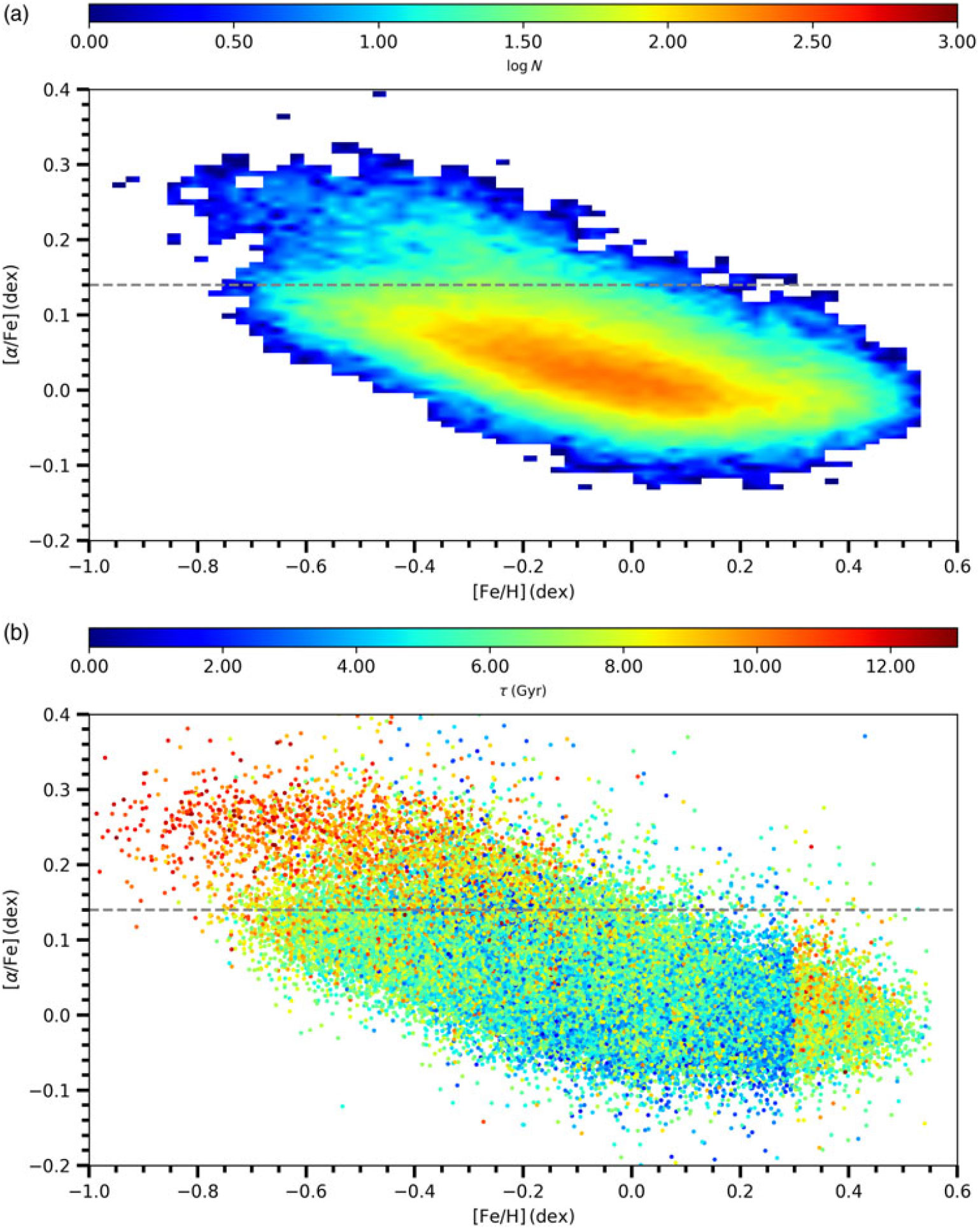
dex. Thus, we adopted the abundance [
$\langle[\alpha/{\rm Fe}]\rangle=0.14$
dex. Thus, we adopted the abundance [ $\alpha$
/Fe] = 0.14 dex as the boundary separating the sample stars in our study as
$\alpha$
/Fe] = 0.14 dex as the boundary separating the sample stars in our study as $\alpha$
-rich and
$\alpha$
-rich and $\alpha$
-poor stars. This procedure is similar to the one in Buder et al. (Reference Buder, Lind and Ness2019), who showed that stars of the high-
$\alpha$
-poor stars. This procedure is similar to the one in Buder et al. (Reference Buder, Lind and Ness2019), who showed that stars of the high- $\alpha$
sequence are older (>8 Gyr) than stars in the low-
$\alpha$
sequence are older (>8 Gyr) than stars in the low- $\alpha$
sequence with the iron abundances
$\alpha$
sequence with the iron abundances $-0.7 \lt [{\rm Fe/H}] \lt +0.5$
dex, and applied their finding to the metal-rich stars which become indistinguishable in the [
$-0.7 \lt [{\rm Fe/H}] \lt +0.5$
dex, and applied their finding to the metal-rich stars which become indistinguishable in the [ $\alpha$
/Fe]
$\alpha$
/Fe] $\,\times\,$
[Fe/H] diagram, as mentioned in the Section 1. Thus, the number of
$\,\times\,$
[Fe/H] diagram, as mentioned in the Section 1. Thus, the number of $\alpha$
-rich and
$\alpha$
-rich and $\alpha$
-poor dwarfs observed in the GALAH survey is
$\alpha$
-poor dwarfs observed in the GALAH survey is $N_1$
= 5 778 and
$N_1$
= 5 778 and $N_2$
= 63 379, respectively. A bimodal distribution in the [
$N_2$
= 63 379, respectively. A bimodal distribution in the [ $\alpha$
/Fe]
$\alpha$
/Fe] $\,\times\,$
[Fe/H] diagram fails due to the less number of
$\,\times\,$
[Fe/H] diagram fails due to the less number of $\alpha$
-rich stars relative to
$\alpha$
-rich stars relative to $\alpha$
-poor ones, that is, 9%.
$\alpha$
-poor ones, that is, 9%.
[ $\alpha$
/Fe]
$\alpha$
/Fe] $\,\times\,$
[Fe/H] diagram for the sample stars with age
$\,\times\,$
[Fe/H] diagram for the sample stars with age $8 \lt \tau\leq 9$
Gyr used for estimation of the abundance [
$8 \lt \tau\leq 9$
Gyr used for estimation of the abundance [ $\alpha$
/Fe]=0.14 dex which separates the stars into
$\alpha$
/Fe]=0.14 dex which separates the stars into $\alpha$
-rich and
$\alpha$
-rich and $\alpha$
-poor categories.
$\alpha$
-poor categories.

[ $\alpha$
/Fe]
$\alpha$
/Fe] $\,\times\,$
[Fe/H] diagram for the sample stars and the horizontal line [
$\,\times\,$
[Fe/H] diagram for the sample stars and the horizontal line [ $\alpha$
/Fe]=0.14 dex which separates them into
$\alpha$
/Fe]=0.14 dex which separates them into $\alpha$
-rich and
$\alpha$
-rich and $\alpha$
-poor categories (a), and the same diagram with colour coded for age (b).
$\alpha$
-poor categories (a), and the same diagram with colour coded for age (b).
4. Summary and discussion
We used the spectroscopic and astrometric data provided from the GALAH DR2 (Buder et al. Reference Buder, Asplund, Duong, Kos, Lind and Ness2018) and Gaia DR2 (Gaia Collaboration Reference Collaboration, Brown and Vallenari2018), respectively, for a large sample of stars to investigate the behaviour of the $[\alpha/{\rm Fe}]$
abundances via two procedures, that is, kinematically and spectroscopically. With the kinematical procedure, we investigated the distribution of the
$[\alpha/{\rm Fe}]$
abundances via two procedures, that is, kinematically and spectroscopically. With the kinematical procedure, we investigated the distribution of the $[\alpha/{\rm Fe}]$
abundances into the thin-disc and thick-disc populations in terms of total space velocity,
$[\alpha/{\rm Fe}]$
abundances into the thin-disc and thick-disc populations in terms of total space velocity, $[{\rm Fe/H}]$
abundance, and age. We applied the following constrains to the total sample of stars (342 682 stars) to obtain a star sample of F–G-type dwarfs with accurate trigonometric parallaxes:
$[{\rm Fe/H}]$
abundance, and age. We applied the following constrains to the total sample of stars (342 682 stars) to obtain a star sample of F–G-type dwarfs with accurate trigonometric parallaxes: $5\,250 \leq T_{eff} \leq 7\,160$
K,
$5\,250 \leq T_{eff} \leq 7\,160$
K, $\log g \geq 4$
(cm s-2),
$\log g \geq 4$
(cm s-2), $\sigma_{\varpi}/\varpi \leq0.05$
, and
$\sigma_{\varpi}/\varpi \leq0.05$
, and $G\leq14$
mag. The number of our sample stars is 69 157. The radial velocities are provided from the GALAH DR2, while the proper motions and trigonometric parallaxes are taken from the Gaia DR2. Radial velocities, proper motions, and distances are combined to obtain space velocity components for the sample stars which are calculated with Johnson & Soderblom (Reference Johnson and Soderblom1987) standard algorithms. Also, the differential rotation correction is applied to the U and V space velocity components.
$G\leq14$
mag. The number of our sample stars is 69 157. The radial velocities are provided from the GALAH DR2, while the proper motions and trigonometric parallaxes are taken from the Gaia DR2. Radial velocities, proper motions, and distances are combined to obtain space velocity components for the sample stars which are calculated with Johnson & Soderblom (Reference Johnson and Soderblom1987) standard algorithms. Also, the differential rotation correction is applied to the U and V space velocity components.
We separated the sample stars into seven sub-intervals of $[\alpha/{\rm Fe}]$
, that is,
$[\alpha/{\rm Fe}]$
, that is, $[\alpha/{\rm Fe}]\leq -0.2$
,
$[\alpha/{\rm Fe}]\leq -0.2$
, $-0.2 \lt [\alpha /{\rm Fe}]\leq 0$
,
$-0.2 \lt [\alpha /{\rm Fe}]\leq 0$
, $0 \lt [\alpha/{\rm Fe}]\leq 0.1$
,
$0 \lt [\alpha/{\rm Fe}]\leq 0.1$
, $0.1 \lt [\alpha/{\rm Fe}]\leq 0.2$
,
$0.1 \lt [\alpha/{\rm Fe}]\leq 0.2$
, $0.2 \lt [\alpha/{\rm Fe}]\leq 0.3$
,
$0.2 \lt [\alpha/{\rm Fe}]\leq 0.3$
, $0.3 \lt [\alpha/{\rm Fe}]\leq 0.4$
, and
$0.3 \lt [\alpha/{\rm Fe}]\leq 0.4$
, and $0.4 \lt [\alpha/{\rm Fe}]\leq 0.7$
dex, and investigated the distributions of the stars therein for four populations, that is, high-probability thin disc (
$0.4 \lt [\alpha/{\rm Fe}]\leq 0.7$
dex, and investigated the distributions of the stars therein for four populations, that is, high-probability thin disc ( $0 \lt TD/D\leq 0.1$
), low-probability thin disc (
$0 \lt TD/D\leq 0.1$
), low-probability thin disc ( $0.1 \lt TD/D\leq1$
), low-probability thick disc (
$0.1 \lt TD/D\leq1$
), low-probability thick disc ( $1 \lt TD/D\leq 10$
), and high-probability thick disc (
$1 \lt TD/D\leq 10$
), and high-probability thick disc ( $TD/D>10$
). We omitted the discussion of nine stars in the sub-interval
$TD/D>10$
). We omitted the discussion of nine stars in the sub-interval $[\alpha/{\rm Fe}]\leq -0.2$
dex. In other sub-intervals of the
$[\alpha/{\rm Fe}]\leq -0.2$
dex. In other sub-intervals of the $[\alpha/{\rm Fe}]$
, the total space velocity interval for the high-probability thin disc stars is
$[\alpha/{\rm Fe}]$
, the total space velocity interval for the high-probability thin disc stars is $0 \lt S_{LSR}\,{\leq}\, 100$
km s-1, while its lower and upper limits shift gradually to higher values when one goes to low-probability thin-disc, low-probability thick-disc, and high-probability thick-disc stars. Also, the number of high-probability thin-disc stars is maximum in all sub-intervals of
$0 \lt S_{LSR}\,{\leq}\, 100$
km s-1, while its lower and upper limits shift gradually to higher values when one goes to low-probability thin-disc, low-probability thick-disc, and high-probability thick-disc stars. Also, the number of high-probability thin-disc stars is maximum in all sub-intervals of $[\alpha/{\rm Fe}]$
abundance. This finding is in contradiction with our expectation, because one expects the number of high-probability thick-disc stars (not the thin disc ones) to dominate in relatively high
$[\alpha/{\rm Fe}]$
abundance. This finding is in contradiction with our expectation, because one expects the number of high-probability thick-disc stars (not the thin disc ones) to dominate in relatively high $[\alpha/{\rm Fe}]$
sub-intervals, such as
$[\alpha/{\rm Fe}]$
sub-intervals, such as $0.3 \lt [\alpha/{\rm Fe}]\leq 0.4$
and
$0.3 \lt [\alpha/{\rm Fe}]\leq 0.4$
and $0.4 \lt [\alpha/{\rm Fe}]\leq 0.7$
dex. However, the percentage of the high-probability thick-disc stars is relatively higher in two high [
$0.4 \lt [\alpha/{\rm Fe}]\leq 0.7$
dex. However, the percentage of the high-probability thick-disc stars is relatively higher in two high [ $\alpha/{\rm Fe}]$
sub-intervals, that is, 28.4
$\alpha/{\rm Fe}]$
sub-intervals, that is, 28.4 $\%$
and 26.6
$\%$
and 26.6 $\%$
in the sub-intervals
$\%$
in the sub-intervals $0.2 \lt [\alpha/{\rm Fe}]\leq 0.3$
and
$0.2 \lt [\alpha/{\rm Fe}]\leq 0.3$
and $0.3 \lt [\alpha/{\rm Fe}]\leq 0.4$
dex, respectively. Another unexpected result is the domination of the high-probability thin-disc stars in the high
$0.3 \lt [\alpha/{\rm Fe}]\leq 0.4$
dex, respectively. Another unexpected result is the domination of the high-probability thin-disc stars in the high $0.4 \lt [\alpha/{\rm Fe}]\leq 0.7$
dex interval, though the number of stars is only 41. Also, the low total space velocities of these stars,
$0.4 \lt [\alpha/{\rm Fe}]\leq 0.7$
dex interval, though the number of stars is only 41. Also, the low total space velocities of these stars, $20.21 \leq S_{LSR} \leq 61.32$
km s-1, and their young ages,
$20.21 \leq S_{LSR} \leq 61.32$
km s-1, and their young ages, $3.71 \leq \tau \leq 7.60$
Gyr, confirm the argument that they belong to the high-probability thin-disc population. However, the domination of the high-probability thin-disc stars in all sub-intervals of
$3.71 \leq \tau \leq 7.60$
Gyr, confirm the argument that they belong to the high-probability thin-disc population. However, the domination of the high-probability thin-disc stars in all sub-intervals of $[\alpha/{\rm Fe}]$
including the high one,
$[\alpha/{\rm Fe}]$
including the high one, $0.4 \lt [\alpha/{\rm Fe}]\leq 0.7$
dex, cannot be generalised. This result is due to the two constrains applied in this study, that is, the limitation of the apparent magnitude (
$0.4 \lt [\alpha/{\rm Fe}]\leq 0.7$
dex, cannot be generalised. This result is due to the two constrains applied in this study, that is, the limitation of the apparent magnitude ( $V \lt 14$
mag) and the intermediate galactic latitudes of the sample stars. Another study which would cover a sample of high-galactic latitude, and apparently faint stars would be rather useful. In this case, we expect a distribution for the sample stars where the high-probability thick-disc stars would dominate in the high
$V \lt 14$
mag) and the intermediate galactic latitudes of the sample stars. Another study which would cover a sample of high-galactic latitude, and apparently faint stars would be rather useful. In this case, we expect a distribution for the sample stars where the high-probability thick-disc stars would dominate in the high $[\alpha/{\rm Fe}]$
abundances.
$[\alpha/{\rm Fe}]$
abundances.
The distributions of the sample stars into the sub-intervals $-0.2 \lt [\alpha/{\rm Fe}]\leq 0$
,
$-0.2 \lt [\alpha/{\rm Fe}]\leq 0$
, $0 \lt [\alpha/{\rm Fe}]\leq 0.1$
,
$0 \lt [\alpha/{\rm Fe}]\leq 0.1$
, $0.1 \lt [\alpha/{\rm Fe}]\leq 0.2$
,
$0.1 \lt [\alpha/{\rm Fe}]\leq 0.2$
, $0.2 \lt [\alpha/{\rm Fe}]\leq 0.3$
,
$0.2 \lt [\alpha/{\rm Fe}]\leq 0.3$
, $0.3 \lt [\alpha/{\rm Fe}]\leq 0.4$
, and
$0.3 \lt [\alpha/{\rm Fe}]\leq 0.4$
, and $0.4 \lt [\alpha/{\rm Fe}]\leq 0.7$
dex show that each of these intervals covers the stars of different populations with different percentages, however. That is, many stars of different populations share the same
$0.4 \lt [\alpha/{\rm Fe}]\leq 0.7$
dex show that each of these intervals covers the stars of different populations with different percentages, however. That is, many stars of different populations share the same $[\alpha/{\rm Fe}]$
abundance. For instance, 731 (35
$[\alpha/{\rm Fe}]$
abundance. For instance, 731 (35 $\%$
) high-probability thin-disc stars and 594 (28.4
$\%$
) high-probability thin-disc stars and 594 (28.4 $\%$
) high-probability thick-disc stars share the abundance interval
$\%$
) high-probability thick-disc stars share the abundance interval $0.2 \lt [\alpha/{\rm Fe}]\leq0.3$
dex, in Table 3. Additionally, 453 (4.4
$0.2 \lt [\alpha/{\rm Fe}]\leq0.3$
dex, in Table 3. Additionally, 453 (4.4 $\%$
) high-probability thick-disc stars share the lower interval
$\%$
) high-probability thick-disc stars share the lower interval $0.1 \lt [\alpha/{\rm Fe}]\leq0.2$
dex with 7584 (73.5
$0.1 \lt [\alpha/{\rm Fe}]\leq0.2$
dex with 7584 (73.5 $\%$
) high-probability thin-disc stars, in the same table. The interpretation of the low
$\%$
) high-probability thin-disc stars, in the same table. The interpretation of the low $[\alpha/{\rm Fe}]$
abundance is generally based on the rich iron abundance of the (thin-disc) stars. According to this argument, the iron-abundance becomes rich in the interstellar medium via the Type Ia supernovae, much later than the formation of the
$[\alpha/{\rm Fe}]$
abundance is generally based on the rich iron abundance of the (thin-disc) stars. According to this argument, the iron-abundance becomes rich in the interstellar medium via the Type Ia supernovae, much later than the formation of the $\alpha$
-elements in the same medium. Then, one should expect rich
$\alpha$
-elements in the same medium. Then, one should expect rich $[\alpha/{\rm Fe}]$
abundance for old/[Fe/H]-poor stars, while the young/[Fe/H]-rich ones would be [
$[\alpha/{\rm Fe}]$
abundance for old/[Fe/H]-poor stars, while the young/[Fe/H]-rich ones would be [ $\alpha/$
Fe]-poor. However, our results cited in this paragraph show that relatively young and iron-rich (high-probability thin-disc) stars and relatively older and poorer in iron abundance (high-probability thick-disc) stars share the same
$\alpha/$
Fe]-poor. However, our results cited in this paragraph show that relatively young and iron-rich (high-probability thin-disc) stars and relatively older and poorer in iron abundance (high-probability thick-disc) stars share the same $[\alpha/{\rm Fe}]$
abundance. This result can be explained as follows: the richness of the
$[\alpha/{\rm Fe}]$
abundance. This result can be explained as follows: the richness of the $[\alpha/{\rm Fe}]$
abundance depends on the richness of the
$[\alpha/{\rm Fe}]$
abundance depends on the richness of the $[\alpha/{\rm H}]$
and [Fe/H] abundances. If these abundances are compatible, then the star is
$[\alpha/{\rm H}]$
and [Fe/H] abundances. If these abundances are compatible, then the star is $[\alpha/{\rm Fe}]$
-poor while (relatively) a large difference between [
$[\alpha/{\rm Fe}]$
-poor while (relatively) a large difference between [ $\alpha/$
H] and [Fe/H] indicates an [
$\alpha/$
H] and [Fe/H] indicates an [ $\alpha/$
Fe]-rich star (we kindly remind to the readers that
$\alpha/$
Fe]-rich star (we kindly remind to the readers that $[\alpha/{\rm Fe}]=[\alpha/{\rm H}]-[{\rm Fe/H}]$
). We separated our sample stars into five
$[\alpha/{\rm Fe}]=[\alpha/{\rm H}]-[{\rm Fe/H}]$
). We separated our sample stars into five $[\alpha/{\rm Fe}]$
intervals, that is,
$[\alpha/{\rm Fe}]$
intervals, that is, $[\alpha/{\rm Fe}]\leq 0$
,
$[\alpha/{\rm Fe}]\leq 0$
, $0 \lt [\alpha/{\rm Fe}]\leq 0.1$
,
$0 \lt [\alpha/{\rm Fe}]\leq 0.1$
, $0.1 \lt [\alpha/{\rm Fe}]\leq 0.2$
,
$0.1 \lt [\alpha/{\rm Fe}]\leq 0.2$
, $0.2 \lt [\alpha/{\rm Fe}]\leq 0.3$
, and
$0.2 \lt [\alpha/{\rm Fe}]\leq 0.3$
, and $0.3 \lt [\alpha/{\rm Fe}]\leq 0.7$
dex and plotted their
$0.3 \lt [\alpha/{\rm Fe}]\leq 0.7$
dex and plotted their $[\alpha/{\rm H}]$
abundances versus [Fe/H] ones in Figure 11 for clarification of our argument. The distributions of the
$[\alpha/{\rm H}]$
abundances versus [Fe/H] ones in Figure 11 for clarification of our argument. The distributions of the $\alpha$
-poor stars (
$\alpha$
-poor stars ( $[\alpha/{\rm Fe}]\leq 0$
and
$[\alpha/{\rm Fe}]\leq 0$
and $0 \lt [\alpha/{\rm Fe}]\leq 0.1$
dex) are almost superposed with the one-to-one straight line, while it deviates gradually from this line when one goes to richer
$0 \lt [\alpha/{\rm Fe}]\leq 0.1$
dex) are almost superposed with the one-to-one straight line, while it deviates gradually from this line when one goes to richer $\alpha$
-abundances. The degree of the deviation corresponds to the difference between the
$\alpha$
-abundances. The degree of the deviation corresponds to the difference between the $[\alpha/{\rm H}]$
and [Fe/H] abundances. Each panel covers [Fe/H]-rich stars as well as stars with
$[\alpha/{\rm H}]$
and [Fe/H] abundances. Each panel covers [Fe/H]-rich stars as well as stars with $-0.7 \lt [{\rm Fe/H}]\leq 0$
dex. Also, the [Fe/H] abundances of the stars with richer
$-0.7 \lt [{\rm Fe/H}]\leq 0$
dex. Also, the [Fe/H] abundances of the stars with richer $\alpha$
-abundances (
$\alpha$
-abundances ( $[\alpha/{\rm Fe}]>0.1$
dex) extends beyond
$[\alpha/{\rm Fe}]>0.1$
dex) extends beyond ${\rm [Fe/H]}=-1$
dex. In summary, we can say that stars with different [Fe/H] abundances may share the same
${\rm [Fe/H]}=-1$
dex. In summary, we can say that stars with different [Fe/H] abundances may share the same $[\alpha/{\rm Fe}]$
abundance, and to be [Fe/H] rich is a sufficient—but not a necessary—condition for a star to be
$[\alpha/{\rm Fe}]$
abundance, and to be [Fe/H] rich is a sufficient—but not a necessary—condition for a star to be $[\alpha/{\rm Fe}]$
poor.
$[\alpha/{\rm Fe}]$
poor.
Distributions of the $[\alpha /{\rm H}]$
abundance against [Fe/H] abundance for five
$[\alpha /{\rm H}]$
abundance against [Fe/H] abundance for five $[\alpha/{\rm Fe}]$
intervals as indicated in Panels (a)–(e). Notice the deviation of the distribution from one-to-one straight line in the direction of increasing of the
$[\alpha/{\rm Fe}]$
intervals as indicated in Panels (a)–(e). Notice the deviation of the distribution from one-to-one straight line in the direction of increasing of the $[\alpha /{\rm Fe}]$
abundance.
$[\alpha /{\rm Fe}]$
abundance.
The domains of the [Fe/H] abundances and the ages for the sample stars are rather large, that is, $-1.3 \lt {\rm [Fe/H]}\leq 0.6$
dex and
$-1.3 \lt {\rm [Fe/H]}\leq 0.6$
dex and $0 \lt \tau \leq 13$
Gyr, respectively. However, when we consider only the
$0 \lt \tau \leq 13$
Gyr, respectively. However, when we consider only the $\langle {\rm[Fe/H]}\rangle \pm 2\sigma$
and
$\langle {\rm[Fe/H]}\rangle \pm 2\sigma$
and $\langle\tau \rangle \pm 2\sigma$
data, the cited domains reduce as follows for four populations: high-probability thin disc:
$\langle\tau \rangle \pm 2\sigma$
data, the cited domains reduce as follows for four populations: high-probability thin disc: $-0.6 \lt {\rm [Fe/H]} \leq 0.4$
dex,
$-0.6 \lt {\rm [Fe/H]} \leq 0.4$
dex, $2 \lt \tau\leq 9$
Gyr; low-probability thin disc:
$2 \lt \tau\leq 9$
Gyr; low-probability thin disc: $-0.7 \lt {\rm [Fe/H]} \leq 0.4$
dex,
$-0.7 \lt {\rm [Fe/H]} \leq 0.4$
dex, $2.5 \lt \tau \leq 10$
Gyr; low-probability thick disc:
$2.5 \lt \tau \leq 10$
Gyr; low-probability thick disc: $-0.8 \lt {\rm [Fe/H]}\leq 0.4$
dex,
$-0.8 \lt {\rm [Fe/H]}\leq 0.4$
dex, $3 \lt \tau \leq 11$
Gyr; and high-probability thick disc:
$3 \lt \tau \leq 11$
Gyr; and high-probability thick disc: $-1 \lt {\rm [Fe/H]}\leq 0.2$
dex,
$-1 \lt {\rm [Fe/H]}\leq 0.2$
dex, $3.5 \lt \tau \leq 12.5$
Gyr, where
$3.5 \lt \tau \leq 12.5$
Gyr, where $\sigma$
is the standard deviation of the data for the cited population, and
$\sigma$
is the standard deviation of the data for the cited population, and $\langle {\rm [Fe/H]}\rangle \pm 2\sigma$
and
$\langle {\rm [Fe/H]}\rangle \pm 2\sigma$
and $\langle \tau\rangle \pm 2\sigma$
cover 95.45
$\langle \tau\rangle \pm 2\sigma$
cover 95.45 $\%$
of the data in question. This procedure eliminates the young/metal-poor stars which are classified as high-probability thick-disc/high-probability thin-disc stars. The most interesting thing in the distribution of the iron abundances and ages of the sample stars is the existence of a large number of metal poor -and old- stars in the high-probability thin-disc population, that is, 1 859 stars with
$\%$
of the data in question. This procedure eliminates the young/metal-poor stars which are classified as high-probability thick-disc/high-probability thin-disc stars. The most interesting thing in the distribution of the iron abundances and ages of the sample stars is the existence of a large number of metal poor -and old- stars in the high-probability thin-disc population, that is, 1 859 stars with ${\rm [Fe/H]} \leq -0.5$
dex and 2 250 stars with
${\rm [Fe/H]} \leq -0.5$
dex and 2 250 stars with $\tau> 9$
Gyr. According to the age–metallicity relation of the sample stars (Figure 6), there is an important number of stars which share the [Fe/H] abundances and ages just cited. That is, we have a sub-sample of high-probability thin-disc stars with compatible [Fe/H] abundance and age with high-probability thick-disc stars. This finding confirms the argument that the metal-poor thin-disc stars were formed at the same epoch of the thick-disc stars with
$\tau> 9$
Gyr. According to the age–metallicity relation of the sample stars (Figure 6), there is an important number of stars which share the [Fe/H] abundances and ages just cited. That is, we have a sub-sample of high-probability thin-disc stars with compatible [Fe/H] abundance and age with high-probability thick-disc stars. This finding confirms the argument that the metal-poor thin-disc stars were formed at the same epoch of the thick-disc stars with $8 \lt \tau \lt 10$
Gyr in a different location of the galaxy (cf. Haywood et al. Reference Haywood, DiMatteo, Lehnert, Katz and Gomez2013). Also, the upper limit [Fe/H] = 0.2 dex claimed for the high-probability thick disc is in agreement with the argument of Haywood et al. (Reference Haywood, Snaith, Lehnert, Di Matteo and Khoperskov2019), who stated that the thick disc enriched up to the solar value 9 Gyr ago. We used the mean of the [
$8 \lt \tau \lt 10$
Gyr in a different location of the galaxy (cf. Haywood et al. Reference Haywood, DiMatteo, Lehnert, Katz and Gomez2013). Also, the upper limit [Fe/H] = 0.2 dex claimed for the high-probability thick disc is in agreement with the argument of Haywood et al. (Reference Haywood, Snaith, Lehnert, Di Matteo and Khoperskov2019), who stated that the thick disc enriched up to the solar value 9 Gyr ago. We used the mean of the [ $\alpha$
/Fe] abundance, that is,
$\alpha$
/Fe] abundance, that is, $\langle[\alpha/{\rm Fe}]\rangle\,=\,0.14$
dex, for the sample stars with age
$\langle[\alpha/{\rm Fe}]\rangle\,=\,0.14$
dex, for the sample stars with age $8 \lt \tau\leq9$
Gyr and
$8 \lt \tau\leq9$
Gyr and $[{\rm Fe/H}]\leq-0.4$
dex to separate them into
$[{\rm Fe/H}]\leq-0.4$
dex to separate them into $\alpha$
-rich and
$\alpha$
-rich and $\alpha$
-poor categories. This value is compatible with the one in Bland-Hawthorn et al. (Reference Bland-Hawthorn, Sharma and Tepper-Garcia2019) claimed for the giants observed in the GALAH survey (their Figure 3).
$\alpha$
-poor categories. This value is compatible with the one in Bland-Hawthorn et al. (Reference Bland-Hawthorn, Sharma and Tepper-Garcia2019) claimed for the giants observed in the GALAH survey (their Figure 3).
We compared the ages estimated in our study with the ones in Buder et al. (Reference Buder, Lind and Ness2019) and Sanders & Das (Reference Sanders and Das2018). The common stars in our study and in Buder et al. (Reference Buder, Lind and Ness2019) are only 1941. The mean of the differences between two sets of ages and the corresponding standard deviation are 0.19 and 2 Gyr, respectively. One can see an agreement in Figure 12 for the two sets of stars with age $\tau \lt 6$
Gyr, while there is a deviation for older ages which probably is due to the different isochrones used in different studies, that is, PARSEC in our study and Darmouth in Buder et al. (Reference Buder, Lind and Ness2019). The mean of the differences between the ages in our study and in Sanders & Das (Reference Sanders and Das2018) for 69 157 stars and the corresponding standard deviation are a bit larger than the former ones, that is, 1.17 and 2.56 Gyr, respectively. As can be seen in Figure 13, the difference between the ages of two studies is larger for the older stars. We compared also the ages in Buder et al. (Reference Buder, Lind and Ness2019) and Sanders & Das (Reference Sanders and Das2018) just to check their agreement (Figure 14). The mean of the differences between the ages of 5 170 common stars in two studies and the corresponding standard deviation are 0.50 and 2.14 Gyr, that is, a bit larger than the ones 0.19 and 2 Gyr cited for the comparison of the ages in our study with the ones in Buder et al. (Reference Buder, Lind and Ness2019). Hence, one can say that the ages estimated in our study are as accurate as the ones appeared in the literature.
$\tau \lt 6$
Gyr, while there is a deviation for older ages which probably is due to the different isochrones used in different studies, that is, PARSEC in our study and Darmouth in Buder et al. (Reference Buder, Lind and Ness2019). The mean of the differences between the ages in our study and in Sanders & Das (Reference Sanders and Das2018) for 69 157 stars and the corresponding standard deviation are a bit larger than the former ones, that is, 1.17 and 2.56 Gyr, respectively. As can be seen in Figure 13, the difference between the ages of two studies is larger for the older stars. We compared also the ages in Buder et al. (Reference Buder, Lind and Ness2019) and Sanders & Das (Reference Sanders and Das2018) just to check their agreement (Figure 14). The mean of the differences between the ages of 5 170 common stars in two studies and the corresponding standard deviation are 0.50 and 2.14 Gyr, that is, a bit larger than the ones 0.19 and 2 Gyr cited for the comparison of the ages in our study with the ones in Buder et al. (Reference Buder, Lind and Ness2019). Hence, one can say that the ages estimated in our study are as accurate as the ones appeared in the literature.
Ages estimated in our study (ordinate axes) versus the ones in Buder et al. (Reference Buder, Lind and Ness2019), (upper panel) and distribution of the age differences in two studies in terms of ages in Buder et al. (Reference Buder, Lind and Ness2019), (lower panel).
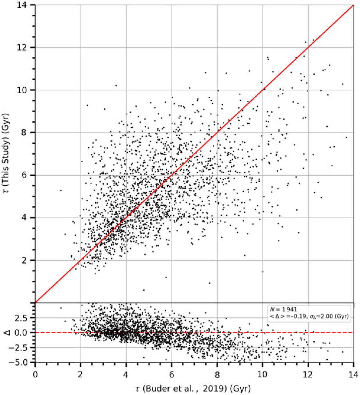
Comparison of the ages estimated in our study and in Sanders & Das (Reference Sanders and Das2018) via the procedure used in Figure 12.
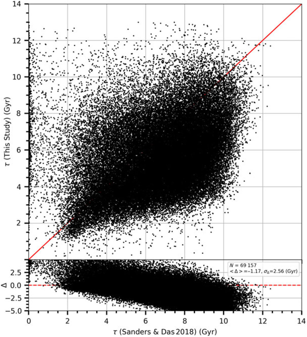
Comparison of the ages in Buder et al. (Reference Buder, Lind and Ness2019) and Sanders & Das (Reference Sanders and Das2018) via the procedure used in Figure 12.
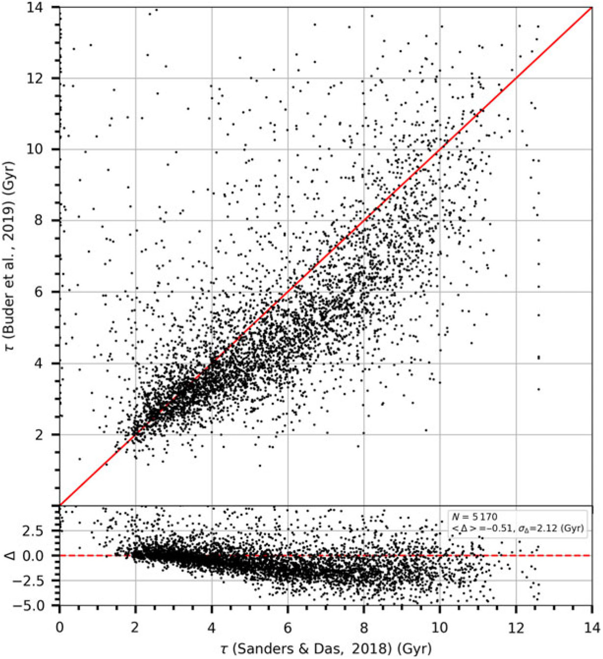
We tested the accuracy of the distances estimated in our study, by using the Gaia DR2 trigonometric parallaxes, by comparing them with the ones estimated via the geometric procedure which is usually used in the literature (Bailer-Jones et al. Reference Bailer-Jones, Rybizki, Fouesneau, Mantelet and Andrae2018). The mean of the differences between the distances estimated by two procedures and the corresponding standard deviation are both 0.01 kpc. Also, one can see in Figure 15 that most of the data fit with the one-to-one straight line, while only a few per cent of them deviate from this line. Actually, the cumulative frequency curve shows that 90% of the data overlap with the curve just cited.
Comparison of the distances for the sample stars estimated via two procedures, that is, Gaia DR2 trigonometric parallaxes (abscissa axes) and geometrically (ordinate axes); 90% of the stars are within 1-kpc distance and they fit with the one-to-one straight line.
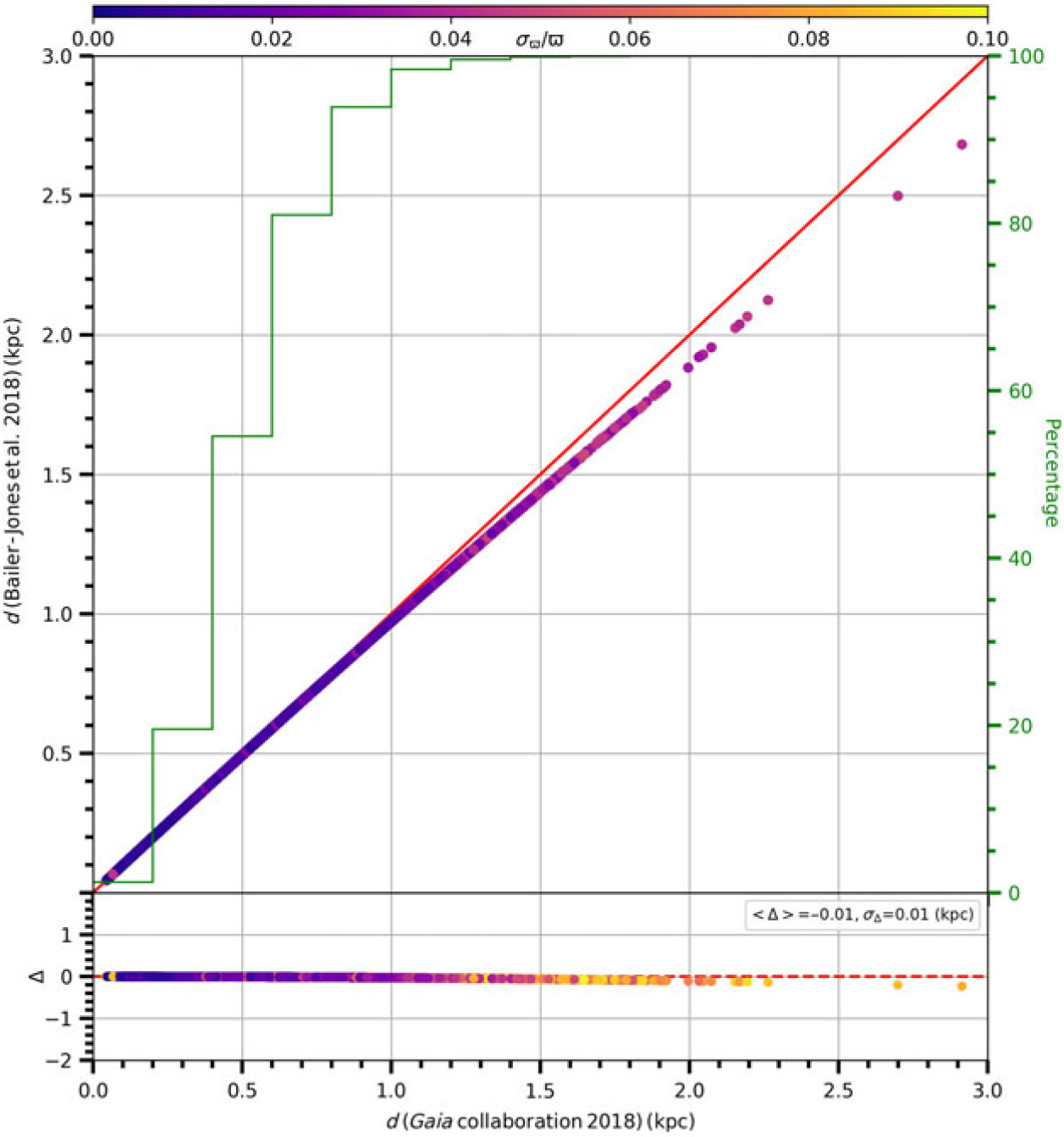
The final comparison is carried out between our data and the ones in a recent study, Casali et al. (Reference Casali, Magrini and Tognelli2019), in the ([ $\alpha/{\rm Fe}$
], [Fe/H], age) space. Our Figure 10(b) and their Figure 13 have almost the same trend. However, the distribution in Casali et al. (Reference Casali, Magrini and Tognelli2019) shows a rather more clear distinction between the
$\alpha/{\rm Fe}$
], [Fe/H], age) space. Our Figure 10(b) and their Figure 13 have almost the same trend. However, the distribution in Casali et al. (Reference Casali, Magrini and Tognelli2019) shows a rather more clear distinction between the $\alpha$
-rich/thick-disc and
$\alpha$
-rich/thick-disc and $\alpha$
-poor/thin-disc populations. Hence, we deduce that the GALAH data we used are perhaps too noisy to show more than a general outline of the underlying relationships.
$\alpha$
-poor/thin-disc populations. Hence, we deduce that the GALAH data we used are perhaps too noisy to show more than a general outline of the underlying relationships.
Acknowledgements
We thank Gerry Gilmore for his valuable comments which improved our paper. This research has made use of NASA’s (National Aeronautics and Space Administration’s) Astrophysics Data System and the SIMBAD Astronomical Database, operated at CDS, Strasbourg, France, and NASA/IPAC Infrared Science Archive, which is operated by the Jet Propulsion Laboratory, California Institute of Technology, under contract with the National Aeronautics and Space Administration. This work has made use of data from the European Space Agency (ESA) mission Gaia (https://www.cosmos.esa.int/gaia), processed by the Gaia Data Processing and Analysis Consortium (DPAC, https://www.cosmos.esa.int/web/gaia/dpac/consortium). Funding for the DPAC has been provided by national institutions, in particular the institutions participating in the Gaia Multilateral Agreement.


