Introduction

Passive-microwave observations make it possible to monitor remote and cloud-covered regions containing large ice masses. On the surfaces of South Greenland (Reference Mote, Anderson, Kuivinen and RoweMote and others, 1993; Reference Steffen, Abdalati and StroeveSteffen and others, 1993; Reference Zwally and FieglesZwally and Fiegles, 1994; Reference Abdalati and SteffenAbdalati and Steffen 1995; Reference TedescoTedesco, 2007), coastal East Antarctica (Reference Liu, Wang and JezekLiu and others, 2006; Reference Picard, Fily and GalleePicard and others, 2007) and Alaska (Reference Ramage and IsacksRamage and Isacks, 2003), more extensive melt and progressively earlier melt onset dates have been detected. Spatial and temporal variations have significant impacts on local and regional hydrology and glacier mass balance. On the Southern Patagonia Icefield (SPI; Fig. 1), the largest temperate ice mass in the Southern Hemisphere, covering approximately 13 000 km² (Reference Naruse and AniyaNaruse and Aniya, 1992), the melt state of the icefield as a whole has never been observed. Few mass-balance data exist for this region, leaving estimates of sea-level rise, climatic trends and hydrologic impacts practically unknown (Reference Rignot, Rivera and CasassaRignot and others, 2003). In this study of the SPI, we investigate how elevation, distance from the coast and latitude affect melt onset and the duration of the spring melt–refreeze cycle as detected by passive-microwave brightness temperature (T _b) measurements in the 37 GHz vertically polarized (V) channel and diurnal amplitude variations (DAV). We then use established thresholds for 37 V T _b (252 K) and DAV (±18 K) to show how T _b and DAV, indicative of melt and melt–refreeze cycles, vary over the entire icefield’s surface both seasonally and interannually. The melt extent and timing influence the mass loss, so this is an important step toward observing mass variations over the entire icefield.

Fig. 1.

SRTM DEM of the SPI with overlying 12.5 km × 12.5 km Equal-Area Scalable Earth Grid (EASE-Grid) pixel classification. The location within the Southern Hemisphere is shown in the inset. Pixel codes are labeled in each gridcell. Pixels 25 (mean elevation 569 m a.s.l.) and 56 (mean elevation 1452 m a.s.l.) (red) are shown in Figure 3. Pixels 30, 31, 52, 53, 110 and 111 (green) are discussed in the text and in Table 2, and pixels 2, 3, 4, 12, 24 and 26 (grey outline) are discussed in the text and exhibit a low-contrast signal. The blue line is the approximate outline of the ice edge (courtesy of G. Casassa).

Passive-Microwave-Derived Melt

Passive-microwave sensors collect microwave radiance as a T _b measurement with sensitivity to the surface characteristics. On glaciers, snowmelt and refreeze processes taking place on and near the surface have dramatic effects on T _b. Snowmelt extent and onset algorithms rely on the significant response of passive-microwave sensors to the presence of a small amount of liquid water (Reference Chang, Gloersen, Schmugge, Wilheit and ZwallyChang and others, 1976; Reference Ulaby, Moore and FungUlaby and others, 1986). These sensors detect microwave emission from the underlying material emanating through the layers of ice and snow that make up the glacier system. Numerical models predict that within a snowpack, up-welling radiation at 37 GHz is predominantly affected by the scattering of snow crystals (Reference Chang, Gloersen, Schmugge, Wilheit and ZwallyChang and others, 1976). Snow is in an intermediate regime between optically thin emission when dry or refrozen (where the sensor collects radiation that has interacted with the entire depth of the ice, firn and snow layers) and optically thick when wet (where the sensor collects radiation only from the surface of last scattering). Volumetric scattering by dry snow and ice particles attenuates the signal, so a lower T _b is measured. The energy scattered also depends on factors such as snow density, thickness and crystal size (Reference Chang, Gloersen, Schmugge, Wilheit and ZwallyChang and others, 1976). For wet snow layers, reduced volumetric scattering and increased absorption increase T _b significantly. T _b is high when the snow is wet because liquid water significantly increases the emissivity (Reference Chang, Gloersen, Schmugge, Wilheit and ZwallyChang and others, 1976).

Several methods were developed for detecting melting snow and ice over Greenland and Arctic sea ice at frequencies near 19 and 37 GHz (wavelengths of 1.58 and 0.82 cm, respectively) utilizing passive-microwave sensors. Early studies used the 19 GHz T _b channel and the mean T _b (T _b – T _{b_mean}) to detect wet snow (Reference Mote, Anderson, Kuivinen and RoweMote and others, 1993; Reference Zwally and FieglesZwally and Fiegles, 1994). Using a 37 GHz horizontally polarized (37H) T _b threshold technique, Reference Mote and AndersonMote and Anderson (1995) investigated melt onset over Greenland. Reference MoteMote (2003) then used this 37H T _b threshold to quantify surface melt, using a positive degree-day approach, to investigate the interannual variability of ablation and surface mass balance over Greenland. Reference Abdalati and SteffenAbdalati and Steffen (1995, Reference Abdalati and Steffen1997) used the 19 GHz horizontally polarized (19H) channel and the 37 GHz vertically polarized channel (37V) to define the cross-polarized gradient ratio (XPGR) or (T _b(19H) − T _b(37V))/(T _b(19H)+T _b(37V)). Reference Steffen, Abdalati and StroeveSteffen and others (1993) used the normalized gradient ratio, (T _b(19H) − T _b(37H))/(T _b(19H)+T _b(37H)), to obtain a wet snow threshold by comparing satellite data and ground measurements. Reference Drobot and AndersonDrobot and Anderson (2001) also developed the advanced horizontal range algorithm (AHRA), which uses temporal variations in 19H and 37H to measure the spatial and temporal variations of snowmelt onset over sea ice from 1979 to 1998.

On the glaciers of southeast Alaska, a new approach for detecting melting snow was proposed by Reference Ramage and IsacksRamage and Isacks (2002), using the difference between the ascending and descending T _b collected via passive-microwave sensor, the Special Sensor Microwave/Imager (SSM/I). This approach uses two co-occurring thresholds, the 37V T _b measurements of 246 K and a diel T _b contrast (DAV) of ±10 K, differentiating a frozen snow surface from a melting surface to determine the melt onset date (Reference Ramage and IsacksRamage and Isacks, 2002). Reference Ramage and IsacksRamage and Isacks (2003) corroborated this methodology based on predominately glacier-fed discharge records for a period overlapping the satellite record. Reference TedescoTedesco (2007) then used this technique to map the areal extent of melting snow over Greenland using 19V and 37V T _b SSM/I channels.

Reference Apgar, Ramage, McKenney and MaltaisApgar and others (2007) refined the T _b and DAV approach for the Advanced Microwave Scanning Radiometer for Earth Observing System (AMSR-E) sensor to retrieve snowmelt onset timing and transition duration in the upper Yukon River basin (Reference Apgar, Ramage, McKenney and MaltaisApgar and others, 2007; Reference Ramage, Apgar, McKenney and HannaRamage and others, 2007). Apgar and others used in situ measurements of temperature taken at 2 hour intervals using automatic data loggers (HOBO, Pro Series) and wetness percent from a snow capacitance probe during AMSR-E overpass to determine thresholds. Melt onset constitutes the first occurrence where one daily T _b is greater than 252 K and the DAV are greater than ±18 K in the 37V channel (Reference Apgar, Ramage, McKenney and MaltaisApgar and others, 2007). This algorithm is applied to the SPI.

Study Site

The SPI is located in the southern Andes, extending from 48°15′ S to 51°35′ S and from 72°30′ W to 74°30′ W (Reference Aniya, Sato, Naruse, Skvarca and CasassaAniya and others, 1997; Reference De Angelis, Rau and SkvarcaDe Angelis and others, 2007). It contains 48 temperate outlet glaciers (Reference Aniya, Sato, Naruse, Skvarca and CasassaAniya and others, 1997), with most glaciers flowing eastwards. All of these glaciers except Frias Glacier and Bravo Glacier calve into bodies of water (Reference Aniya, Sato, Naruse, Skvarca and CasassaAniya and others, 1997). There is a scarcity of climatological stations on, and adjacent to, the SPI (Reference Rasmussen, Conway and RaymondRasmussen and others, 2007). The SPI is influenced by both Antarctic and mid-latitude atmospheric circulation patterns and a diversity of climatic environments (Reference Warren and SugdenWarren and Sugden, 1993). Prevailing westerly winds from the Pacific Ocean combined with the steep Andean terrain generate high precipitation on the SPI’s western front, with accumulation diminishing towards the east (Reference Rivera and CasassaRivera and Casassa, 2004). Thus, mass balance on the west is dominated by winter snow accumulation while the east undergoes significant summer ablation. Both the western and eastern regions of the SPI experience high mass turnover rates with significant inter-annual variability in accumulation and ablation (Reference Bamber and RiveraBamber and Rivera, 2007).

Research efforts involving the SPI have increased substantially during the last decade, but many glaciological variables, especially mass balance, are still poorly understood (Reference De Angelis, Rau and SkvarcaDe Angelis and others, 2007). Reference Aniya, Sato, Naruse, Skvarca and CasassaAniya and others (1997) investigated terminus variations for the 48 outlet glaciers of the SPI based on maps, aerial photographs and satellite imagery. Their study demonstrates that the termini of many glaciers in the region exhibit a general pattern of recession, but differences are evident from one glacier to another. Reference Rignot, Rivera and CasassaRignot and others (2003) used a digital elevation model (DEM)-differencing approach to achieve the first regional mass-balance study. From 1975 to 2000, glacier loss yielded 0.042 ± 0.002 mm a⁻¹ sea-level equivalent (SLE), with a higher rate of 0.105 ± 0.011 mm a⁻¹ SLE during the 1995–2000 period (Reference Rignot, Rivera and CasassaRignot and others, 2003). Another recent study estimates the combined contribution of the Northern and Southern Patagonia Icefields to sea-level rise using forward modeling and 5 years of Gravity Recovery and Climate Experiment (GRACE) data (Reference Chen, Wilson, Tapley, Blankenship and IvinsChen and others, 2007). After correcting for glacial isostatic adjustment and hydrological effects, Reference Chen, Wilson, Tapley, Blankenship and IvinsChen and others (2007) estimated a contribution of 0.078 ± 0.031 mm a⁻¹ SLE, comparable to the rates obtained by Reference Rignot, Rivera and CasassaRignot and others (2003). We use twice daily passive-microwave measurements covering the entire icefield to generate a spatially complete and temporally dynamic high-resolution reconstruction of melt dynamics on the icefield from 2002 to 2008. We also investigate which regions are dominated by a seasonal T _b distribution and those regions that experience interspersed wet snow, frozen snow or melting and refreezing snow throughout the year.

Data

This investigation analyzes data from the AMSR-E, a six-frequency (6.925, 10.650, 18.700, 23.800, 36.500 and 89.000 GHz) dual polarized total-power conically scanning passive-microwave radiometer on board NASA’s Aqua satellite (Reference KawanishiKawanishi and others, 2003). We focus on austral hydrological years (Table 1) from 2002 to 2008. Three datasets were acquired: AMSR-E/Aqua Level-2A global swath spatially resampled T _b (http://nsidc.org/data/ae_l2a.html); a 3 arcsec (90 m resolution) DEM image from the Shuttle Radar Topography Mission (SRTM) (Reference Farr and KobrickFarr and Kobrick, 2000); and drainage basin delineations used to infer the Andean topographic divide (http://eros.usgs.gov/products/elevation/gtopo30/hydro/sa_basins.html). Using Geographic Information System (GIS) software, multiple 3 arcsec (90 m) SRTM DEMs were acquired and joined to produce the SPI data used in this investigation. The SPI extent was determined by placing the Equal-Area Scalable Earth Grid (EASE-Grid) over the SRTM DEM. Glacier boundaries were double-checked with the few available cloud-free Advanced Spaceborne Thermal Emission and Reflection Radiometer (ASTER) images and an ice-margin delineation (courtesy of G. Casassa). A total of 107 high-resolution (12.5 km × 12.5 km) EASE-Grid pixels cover the SPI (Fig. 1). Using GIS grid overlay software, each pixel was individually clipped out of the SRTM DEM to extract spatial statistics. The elevation histogram and mean, minimum and maximum elevations were used to characterize each pixel.

Table 1.

Date ranges for austral hydrologic seasons 2002–08

AMSR-E L2A global swath spatially resampled T _b measurements for 2002–08 were acquired free of cost from the Warehouse Inventory Search Tool (WIST) website (http://wist.echo.nasa.gov/∼wist/api/imswelcome) provided by NASA. The US National Snow and Ice Data Center (NSIDC) provides an AMSR-E swath-to-grid toolkit (AS2GT) (http://nsidc.org/data/tools/pmsdt/as2gt.html) with software tools to subset and grid L2A AMSR-E swath data at any spatial resolution and map projection. AMSR-E data are interpolated to the output EASE-Grid, Southern Hemisphere projection, from swath space using an inverse-distance squared method. The EASE-Grid has a nominal 12.5 km × 12.5 km grid spacing. The instantaneous field-of-view dimensions are approximately 27 km × 16 km at 37 GHz (mean spatial resolution of 12 km). EASE-Grid tools are provided by the NSIDC (http://nsidc.org/data/ease/tools.html). The NSIDC also provides Interactive Data Language (IDL) routines and map projections for geolocation and conversion tools to use with EASE-Grid datasets.

AMSR-E L2A data are in Hierarchical Data Format (HDF). The NSIDC tools AMSR-E_L2A_togs and the gsgrid (South-ern Hemisphere high-resolution grid) procedures were used to process the raw AMSR-E data from HDF format to gridded T _b. Data were gridded to 12.5 km × 12.5 km EASE-Grid AMSR-E files for T _b in 10.7, 18.7, 23.8, 36.5 and 89.0 GHz for both horizontal and vertical polarizations containing the time and date of satellite acquisition. An IDL program then read in all the gzipped EASE-Grid AMSR-E output files and extracted T _b in all channels and polarizations for the 107 high-resolution pixels covering the SPI. This program also wrote text files for each pixel containing all T _b measurements ordered sequentially for a year and acquisition time in decimal days. Using the IDL environment, both T _b and DAV (the difference between the daily maximum and minimum T _b) structures were created for all 107 pixels and tagged according to channel, acquisition time and the spatial statistics extracted from the SRTM DEM.

Methods

Quantifying melt onset, transition end and spring melt–refreeze duration

37V T _b and DAV data are used to capture the onset and duration of melt–refreeze cycles and the onset of sustained melting within each austral hydrologic year from 2002 to 2008. The first step was to determine whether existing thresholds were applicable to this environment. AMSR-E T _b and DAV thresholds of 252 K and ±18 K in the 37V channel appear to be robust on the SPI based on the T _b distribution (histogram plots) of all snow-covered high-elevation pixels (Fig. 2). The 37V 252 K threshold corresponds to the low count separating the two populations of lower T _b values of a frozen surface and a higher T _b value of a wet surface. The DAV capture the diurnal fluctuation of liquid water content at the spring melt onset. At night a refreezing snow surface forms larger grains, which increase volumetric scattering, and tends to have a lower T _b than fresh snow (Reference RamageRamage, 2001). The T _b and DAV thresholds detect the presence of liquid water, and a large diurnal T _b range indicates the process of melting and refreezing.

Fig. 2.

Frequency histograms of twice daily 37V T _b measurements for 2002–08 for all pixels (thick black curve) and individual pixels with minimum elevations >1200 ma.s.l. (thin black curves). Histogram shapes are bimodal, typical of other large ice masses such as the icefields of Alaska and the Greenland ice sheet. The left distribution and right distributions distinguish T _b from dry and refrozen snow (180–252 K) vs wet snow (>252 K). The T _b that separates these two conditions is the T _b threshold (252 K).

The AMSR-E T _b signature is sensitive, and short-term variability makes it difficult to automate transition end. For instance, within a prolonged melt period, there are notable instances where T _b fluctuates similar to the transition period, but for a brief duration. This synoptic variability complicates pinpointing the correct transition end date. In this investigation, rather than using transition end, ‘sustained melt’ is defined because the influence of this synoptic variability on melt has yet to be determined. Sustained melting begins when T _{b_min} exceeds 252 K on 6 out of 7 consecutive days. The first day of the sequence is the sustained melt onset date. The spring melt–refreeze duration is comparable to the transition period (Reference Apgar, Ramage, McKenney and MaltaisApgar and others, 2007), but is calculated as the number of days between the melt onset and sustained melt onset.

Figure 3 illustrates when 37V T _b and DAV thresholds indicate melt onset, transition duration and transition end for pixels 25 (mean elevation 569 m a.s.l.) and 56 (mean elevation 1452 m a.s.l.) during the 2007/08 hydrologic year (begins on 1 July in the Southern Hemisphere). Melt onset (solid line) occurs in the 37V channel once T _{b_max} is greater than 252 K and the DAV are greater than ±18 K. After melt onset, the transition period is when T _b and DAV fluctuate as the surface undergoes diel (vertical) melting and refreezing. The transition end date occurs when there is consistent surface melting. This is defined as when T_{b_min} remains above the 252 K threshold for a consecutive period of time (6 days in this study; dashed line). The T _b signature re-enters this diel fluctuation cycle again as temperatures drop in austral autumn (Fig. 3).

Fig. 3.

2007/08 hydrologic year 37V T _b (black curve) and DAV (dashed curve) time series for pixels with different mean elevations on the SPI. (a) Low-elevation pixel 25 (mean elevation 569 m a.s.l.) and (b) higher-elevation pixel 56 (mean elevation 1452 m a.s.l.). A histogram of elevations (m) extracted from the 3 arcsec SRTM DEM for each pixel is shown next to the time series. After austral winter temperatures begin to rise, when T _b > 252 K and DAV > ±18 K, it signifies the melt onset date (solid line) where there is daytime melting and night-time refreezing. This period is referred to as the transition period. As temperatures increase, daily fluctuations cease and daytime T _b remains above 252 K for a consecutive period of time, indicating the end of the transition period (dashed line). In this example, the timing and duration of melt are affected by elevation. Pixel 25 experiences an earlier melt onset and a shorter transition period relative to pixel 56.

Quantifying melt extent

Each pixel on the icefield was classified according to its 37V T _b histogram distribution. Two general categories are defined for the SPI based on their histograms. The first type includes pixels with a bimodal distribution, with the established 252 K melt threshold constituting the low-count T _b between the two large populations of high or low T _b. The second type includes pixels with an asymmetrical distribution that is skewed to the right and peaks 4–8 K above the established threshold (Fig. 4). Four types of melt regimes can be derived from histogram shapes: (1) a bimodal distribution with a peak at low T _b (Fig. 5a); (2) an equal bimodal distribution (Fig. 5b); (3) a bimodal distribution with a peak at high T _b (Fig. 5c); and (4) an asymmetrical distribution (Fig. 5d). The bimodal histogram with a peak at low T _b indicates a longer period spent frozen relative to time spent wet. Conversely, the bimodal histogram with a peak at high T _b indicates a longer period spent melting and wet relative to time spent dry. The asymmetrical distribution indicates that the surface is wet and melting well over 50% of the time. The distribution of histogram types is mapped for each pixel over the SPI (Fig. 6).

Fig. 4.

Frequency histograms of twice daily 37V T _b measurements for pixels 25 and 56 from 2002 to 2008. Pixel 56 has a bimodal distribution. The left and right distributions distinguish T _b between dry and refrozen snow and wet snow. The T _b that separates these two conditions is the T _b threshold (252 K). Pixel 25 and the inset showing a histogram of all 37V T _b measurements from all of the SPI pixels for this period display an asymmetrical distribution that is skewed to the right and peaks above the T _b threshold.

Fig. 5.

37V T _b histograms differentiate four types of melt regimes over the SPI. The 37V T _b threshold (252 K) is shown as a vertical line. (a) The bimodal peak at a low T _b value indicates that the snow is dry three-quarters of the time. (b) An equal bimodal distribution can be interpreted as the left distribution being T _b of dry snow in the winter and the right distribution being T _b of melting snow in the summer. (c) The bimodal histogram with a peak at high T _b indicates a longer period of time melting and wet relative to time spent dry. (d) The normal distribution peaks near or above the T _b threshold and indicates that the surface is wet and melting for most of the time.

Fig. 6.

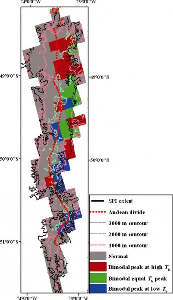
Map showing distribution of melt regimes based on histogram type across the SPI. Bimodal distributions with a peak at high T _b occur in the northeast (red). Bimodal distributions with equal peaks are in the northeast and middle sector on pixels with a mean elevation below 1500 m a.s.l. (green). Bimodal distributions with a peak at low T _b are in the middle and southern sector on pixels with mean elevations >1500 m a.s.l. (blue). The normal and asymmetrical shape is directly west of the divide and retains this shape with varying latitude and mean elevation (gray). The black line is the approximate outline of the ice edge.

The spatial distribution of seasonal variations in T _b distinguishes regions with high-contrast from those with low-contrast (typically moisture-dominated) surface characteristics. We mapped the percentage time a pixel is above the 252 K threshold per season and year as a way to discriminate high- and low-contrast regions. Low-contrast regions indicate regions of high surface moisture which results from maritime air masses, and high-contrast regions are dominated by a more continental signal (Fig. 7).

Fig. 7.

Seasonal and interannual distributions of melt throughout the SPI for hydrologic years 2002–07. The melt maps for each season are based on the percentage of time both the daily T _{b_max} and T _{b_min} are greater than the 37V T _b threshold (0% (blue) to 100% (red)) for each season within the austral hydrologic years from 2002 to 2007. The annual maps are calculated based on the percentage of time both the daily T _{b_max} and T _{b_min} are greater than the 37V T _b threshold (0% (black) to 100% (white)) for each year and thus also have a low DAV. Seasonally and annually there are pixels with a dominant signature characterizing melting (includes wetness due to rain), frozen, or melting and refreezing. Depending which is dominant, the pixel is considered low-contrast, where the T _b signal is primarily influenced by maritime air masses (T _{b_min} > 252 K 75% of the time), or high-contrast, where the T _b’s show that surface moisture is lower and the region has a more continental climate.

Results

Melt onset

Annual time series of T _b and DAV show a seasonal T _b cycle with short-term variability events occurring over the whole icefield. Later we distinguish between areas that are more dominated by low-contrast seasonal conditions from areas with high-contrast seasonal temperature fluctuations. Other regions experience sustained periods of high DAV fluctuations, especially in the high-elevation areas. We look in more detail at pairs of pixels at different mean elevations on either side of the divide, in the northern, middle and southern parts of the icefield.

Melt onset, sustained melt onset and the spring melt–refreeze duration vary for these six pixels (Table 2). Melt onset is typically in late austral winter or early spring beginning in July for pixels north of 48°50′ S, with mean elevations below 1500 m and located west of the divide. Here the spring melt–refreeze cycle lasts 57 days (except pixel 30). For pixel 30, sustained melt onset starts on 26 July. The comparable pixel east of the divide melts on 15 September with a melt–refreeze duration of 31 days. In the middle of the icefield, melt onset on the west is 7 days earlier relative to the east, whereas in the south it is 75 days earlier in the west. The last wave of melt onset occurs in November for pixels east of the divide and distant from the equator. Sustained melt onset south of 48°50′ S occurs in December and January, with melt onset occurring 25–35 days earlier for pixels west of the divide. Some pixels do not fit this model, typically those with mean elevations greater than 1500 m and located to the east of the divide. These pixels never stop the diel melt–refreeze process and express the transition period for the whole austral summer until April.

Table 2.

Pixel characteristics for selected pixels discussed in the text. See Figure 1 for the locations of these pixels. All dates listed are for the austral hydrologic year 2007/08

Melt extent

For the SPI, T _b histogram shapes fall into two main classes: those with bimodal distributions peaking at low, equal or high T _b and those skewed to the right with an asymmetrical peak 4–8 K above the 252 K T _b threshold. The characteristic bimodal shape is typical of pixels east of the Andean divide. Figure 6 shows the locations of these different types of T _b distributions on the SPI. Bimodal distributions with a peak at high T _b occur in the northeast and southeast. Bimodal distributions with a peak at low T _b are in the middle sector on pixels with mean elevations above 1500 m. Bimodal distributions with equal peaks are in the northeast on pixels with a mean elevation below 1500 m. West of the topographic divide (dotted line in Fig. 6), histograms remain asymmetrical and skewed to the right. They preserve this shape with increasing latitude and elevation.

For all pixels, distance from the coast (windward or leeward position relative to the divide) plays a critical role in 37V T _b histogram distribution shape. Latitudinal variations have no effect on the melt signature on the windward side of the SPI, from 48° S to 51° S, spanning a distance of ∼350 km. On the leeward side, the T _b histograms change with increasing latitude and elevation. For pixels with a mean elevation above 1500 m, the bimodal distribution peaks at lower T _b. The bimodal distribution peaks at higher T _b values for pixels close to the equator and it shifts to a peak at lower T _b values for those pixels that are more distant (southerly).

The percentage time above the melt threshold for each hydrologic season within each hydrologic year, and for each year, is used to determine the distribution of melt (Fig. 7). In winter the majority of pixels have daily T _b below 252 K throughout the season except in the northwest, where a few pixels spend 20–50% of the time melting. In spring, melt days increase in number on the windward side of the Andes and the leeward surface remains frozen. The majority of pixels throughout the icefield melt during summer. The distribution of melt diminishes dramatically from summer to fall. More pixels are below 252 K in fall relative to spring. These maps of total melt show very little regional seasonal or interannual variability.

The annual maps show that the windward side has a greater percentage of melt days than the leeward side. In the northern SPI, pixels 2, 3, 4, 12, 24 and 26 spend over 75% of the time above the T _b threshold. For these pixels, T _b is not driven by temperature changes and we interpret them as low-contrast pixels dominated by maritime conditions. The remaining pixels show a high-contrast T _b signal where surface moisture is lower and the region has a more continental climate. East of the divide, between −48.8° S and −50.8° S and at elevations above 1500 m, transition and non-melt days occur interspersed throughout the hydrologic year.

The variation of melt timing for the pixels least affected by maritime climate is summarized for the period of record. For pixels east of the divide, T _b histograms have a bimodal distribution, with the 252 K melt threshold constituting the low-count T _b between the two large populations of high and low T _b. For these areas, temperature is the dominant mass-balance control and they lack frequent rainfall. Figure 8a shows the mean spring melt–refreeze duration for all pixels and for pixels with bimodal distributions for hydrologic years 2002–07. For all pixels, the mean spring melt–refreeze period has changed by −10 days a⁻¹ and it is −16 days a⁻¹ for pixels with bimodal distributions. The mean spring melt–refreeze period has changed by −22, −15 and −13 days a⁻¹ for those pixels with bimodal distribution with peaks at low T _b, equal T _b and high T _b, respectively. Figure 8b shows the spring melt–refreeze duration for all pixels and years. Interannual variability exists and a decreasing duration of the spring melt–refreeze period is apparent from hydrologic years 2002–07.

Fig. 8.

(a) The mean spring melt–refreeze duration, defined as the difference between the sustained and melt onset dates for all pixels (thick black line) and for pixels with bimodal distributions (thin grey line) for hydrologic years 2002–07. Pixels that have a bimodal distribution with a peak at high T _b are in red, those with a peak at low T _b are in blue, and those with an equal bimodal distribution are in green. (b) Maps showing the spatial and temporal variation of spring melt–refreeze duration for each pixel. These maps demonstrate that the spring melt–refreeze duration (red (0 days) to cyan (150 days) to white (250 days), has shortened regionally from 2002 to 2007.

Discussion

Quantifying the annual pattern of 37V T _b observations, indicative of surface moisture, shows where T _b’s are driven by seasonal temperature changes. This facilitates spatially distributed interpretations of surface melt and melt–refreeze cycles in a region of high climatic and topographic diversity such as the SPI. The AMSR-E signal is seasonal east of the divide, which makes it possible to interpret melt timing, extent and duration. In this region, melt starts in mid-September; regions with higher mean elevations that are also farther from the equator start to melt in December. West of the divide, melt and sustained melt onset always occur significantly earlier relative to the east. In the northwest region of the icefield, melt onset occurs in July, with later melt onset dates occurring in early September. It is worth noting that the observations of melt and sustained melt onset west of the divide may be complicated by accumulation rates and rain-induced surface moisture. Pixels west of the divide all have 37V T _b histograms with asymmetrical distributions. High precipitation rates on the windward side of the SPI most likely contribute to this shape. Reference Mote and AndersonMote and Anderson (1995) simulated 37H T _b and April emissivity over the Greenland ice sheet and found higher emissions in the southeast where accumulation rates are high. Rainwater in the surface will also increase the surface emissivity and hence T _b. The stability of this asymmetrical shape with changes in latitude and elevation supports this conclusion. On the southern sector of the icefield, T _b and DAV fluctuations are of lesser magnitude, perhaps because this region has a lower mean elevation and is more homogeneous. Mapping ice- and snow-covered regions based on their histogram shape, either asymmetrical high-T _b bimodal, low-T _b bimodal or equal-T _b bimodal, is useful for accurate interpretations of melt timing and duration trends.

The melt signature can be tested for its applicability to predict melt onset and runoff timing. Reference Ramage and IsacksRamage and Isacks (2003) and Reference KopczynskiKopczynski and others (2008) showed the predictive capability of the transition end date for determining peak runoff timing in streams fed predominantly by glaciers in Alaska. During the spring transition period, daily melting and refreezing occurs and melt is retained within the glacial system. It is not until constant melting starts, as indicated by T _b > 252 K and a low DAV for a consecutive period of time, that melt permeates and runoff is detected down-glacier. A strong relationship is found in Alaska between the end of the melt–refreeze cycle and snowmelt flood timing (Reference KopczynskiKopczynski and others, 2008). If a significant relationship between the timing of AMSR-E-derived melt and rises in streamflow exists, subtracting the lag time will show the T _b signal history up to meltwater release. Ultimately, this tool will help us determine the degree to which storms and melt events influence runoff.

Surface melt extent and timing are intimately tied to internal dynamics within temperate glacial systems. Figure 8 shows the spring surface melt–refreeze cycle becoming shorter from 2002 to 2008 for regions that have temperature as their dominant control on melt. On the Greenland ice sheet, Reference Zwally, Abdalati, Herring, Larson, Saba and SteffenZwally and others (2002) found ice acceleration when the duration of surface melting increased. Changes in the spring melt–refreeze period will affect ice movement via changes in meltwater storage, and the timing and volume of runoff to streams that are predominantly fed by the SPI.

Conclusions

Daily AMSR-E brightness temperatures over the SPI show coherent T _b and DAV on an annual basis. Changes in latitude, elevation and location relative to the spine of melt on the Andes affect the timing and characteristics of melt. Melt onset is highly variable for different regions and elevations throughout the icefield. Melt onset occurs in September, with earlier onsets for pixels west of the divide. Sustained onset starts in September and October in the north and in December and January below 48°50′ S. Pixels west of the divide begin sustained melting 23–35 days earlier.

These melt characteristics can also be interpreted through T _b histogram shapes, which show distinct melt regimes on the windward and leeward side of the Andes. Pixels on the windward side of the Andes have AMSR-E 37V T _b histograms that are asymmetrical in shape, skewed to the right and peak 4–8 K above 252 K. Even with increases in latitude and elevation, the histograms retain this shape. We interpret this as sites dominated by melt- or rain-induced surface moisture and the region’s higher accumulation rate. Pixels on the leeward side have 37V T _b histograms with a bimodal distribution. The 252 K T _b threshold separates the higher cluster of T _b, indicative of wet snow, from T _b measurements with <1% liquid water content. With increasing elevation, T _b count increases at the lower T _b values. This distribution is typical of other large ice masses such as the icefields of Alaska and Greenland. On the SPI, regions with bimodal peaks at high T _b include northeast and southeast regions where mean elevations are <1500 m a.s.l.

For each hydrologic year from 2002 to 2007, the icefield surface is frozen in winter and fall and is wet and melting in summer. In spring the windward side of the Andes is wet and melting while the leeward side remains frozen. In the northwest sector of the SPI T _b’s remain above the threshold from spring to fall, and spend 50% of the time above 252 K in winter. The dominant T _b distribution over the SPI shows high-contrast characteristics, with large periods of melt, non-melt and melt–refreeze cycles within the T _b time series, except in the northwest which has a low-contrast signature, probably dominated by the maritime climate.

For all pixels, the mean spring melt–refreeze period has changed by −10 days a⁻¹,and by −16 days a⁻¹ for pixels with bimodal distributions. The mean spring melt–refreeze period is decreasing for those pixels with bimodal distribution with peaks at low T _b (−22 days a⁻¹ change). Although spatial and temporal variability exists, a decreasing duration of the spring melt–refreeze period is apparent from hydrologic years 2002–07.

Melt extent, timing, trends and their relationship to runoff timing and mass balance are significant factors to monitor as the icefields are exposed to a changing climate. Quantifying the influence of the melt on mass balance, runoff and surface–atmosphere interactions aids modeling efforts to calculate the volumetric loss rates for all large temperate glacial systems.