


1 Introduction
Multiple regression is a commonly used tool to study the linear relationship between a criterion variable and a set of predictor variables. To report the results of multiple regression, researchers always provide not only R 2 (i.e., the proportion of variance of the criterion variable explained by the set of predictor variables) but also each of the estimated regression coefficients. To test the significance of a regression coefficient, the estimated regression coefficient and the associated standard error estimate can be used to either compute the t statistic or construct the confidence interval (CI).
In social and behavioral sciences, many variables are measured on arbitrary scales (e.g., Likert scales) and thus lack substantive meanings. With the motivation to compare the relative importance of predictor variables in relation to the criterion variable, researchers often focus on the standardized regression coefficients, rather than the unstandardized regression coefficients. For example, if we want to study whether income and perceived social support have a similar impact in predicting life satisfaction, it is better to compare the magnitude of standardized regression coefficients, whereas it is not meaningful to compare the unstandardized regression coefficients because the magnitude of unstandardized regression coefficients can be arbitrarily manipulated with the scales that measure income and perceived social support, separately. Consequently, the results typically reported for regression analysis in social sciences include the point estimates of standardized regression coefficients, the associated standard error estimates, the t values, and the p-values. Nonetheless, such a reporting practice is often problematic. Specifically, several textbooks (e.g., Cohen et al., Reference Cohen, Cohen, West and Aiken2003, p. 86; Harris, Reference Harris2001, p. 80; Hays, Reference Hays1994, p. 709) show the formula (referred to as the textbook formula hereafter) that the standard error estimate for a standardized regression coefficient can be obtained by transforming the corresponding standard error estimate for the unstandardized regression coefficient using the sample standard deviations of the criterion variable and the corresponding predictor variable. Howell (Reference Howell2013) did not show the textbook formula but asserted that the same test statistic (i.e., t value) would be obtained no matter whether we test the unstandardized regression coefficient or the standardized regression coefficient (see the last sentence of the second last paragraph on page 521). Nevertheless, Yuan and Chan (Reference Yuan and Chan2011) and Jones and Waller (Reference Jones and Waller2013, Reference Jones and Waller2015) pointed out that the textbook formula (and Howell's assertion based on it) is incorrect and should not be used to compute the standard error estimates for standardized regression coefficients. In the literature, different methods have been developed to solve this problem. However, no analytic method has been proposed when interaction terms of standardized variables are involved in the regression models. As interaction terms of standardized variables are frequently examined in social and behavioral sciences (Aiken & West, Reference Aiken and West1991), it is imperative to adopt the correct method for standard error estimation for accurate statistical inferences. Therefore, the present article aims to introduce an analytic approach to regression with or without interaction terms. In the rest of this section, we first review the problem of the textbook formula as well as the methods that have been developed to solve this problem. Next, we point out the gap in the literature when the regression model is extended to involve interaction terms of standardized variables, followed by the aim and advantages of our analytic approach.
1.1 The problem of textbook formula
Let the regression model be
 $$\begin{align*}{y}_i={b}_0+{b}_1{x}_{i1}+\cdots +{b}_p{x}_{ip}+{\varepsilon}_i,\kern0.36em i=1,2,\cdots, n,\kern0.36em \mathrm{Var}\left({\varepsilon}_i\right)={\sigma}_{\varepsilon}^2,\end{align*}$$
where yi
is the unstandardized criterion variable, xij
(j = 1, …, p) is the jth unstandardized predictor variable, εi
is the error, b
0 is the intercept, and bj
is the jth unstandardized regression coefficient. Let $\mathbf{b}={\left({b}_1\kern0.5em {b}_2\kern0.5em \cdots \kern0.5em {b}_p\right)}^{\prime }$
be a column vector of unstandardized regression coefficients. The least squares estimate of b is
$\mathbf{b}={\left({b}_1\kern0.5em {b}_2\kern0.5em \cdots \kern0.5em {b}_p\right)}^{\prime }$
be a column vector of unstandardized regression coefficients. The least squares estimate of b is $\widehat{\mathbf{b}}={\left(\begin{array}{cccc}{\widehat{b}}_1& {\widehat{b}}_2& \cdots & {\widehat{b}}_p\end{array}\right)}^{\prime }={\mathbf{S}}_{xx}^{-1}{\mathbf{s}}_{xy}$
, where
$\widehat{\mathbf{b}}={\left(\begin{array}{cccc}{\widehat{b}}_1& {\widehat{b}}_2& \cdots & {\widehat{b}}_p\end{array}\right)}^{\prime }={\mathbf{S}}_{xx}^{-1}{\mathbf{s}}_{xy}$
, where ${\mathbf{S}}_{xx}=\left(\begin{array}{cccc}{s}_1^2& & & \\ {}{s}_{21}& {s}_2^2& & \\ {}\vdots & \vdots & \ddots & \\ {}{s}_{p1}& {s}_{p2}& \cdots & {s}_p^2\end{array}\right)$
is the sample covariance matrix of x
i1, …, xip
and s
xy
is a column vector of covariances between x
i1, …, xip
and yi
. Then, the estimate of the jth standardized regression coefficient, denoted by βj
, is given by
${\mathbf{S}}_{xx}=\left(\begin{array}{cccc}{s}_1^2& & & \\ {}{s}_{21}& {s}_2^2& & \\ {}\vdots & \vdots & \ddots & \\ {}{s}_{p1}& {s}_{p2}& \cdots & {s}_p^2\end{array}\right)$
is the sample covariance matrix of x
i1, …, xip
and s
xy
is a column vector of covariances between x
i1, …, xip
and yi
. Then, the estimate of the jth standardized regression coefficient, denoted by βj
, is given by
 $$\begin{align}{\widehat{\beta}}_j=\frac{s_j}{s_y}{\widehat{b}}_j,\end{align}$$
where ${s}_j=\sqrt{s_j^2}$
is the sample standard deviation of xij
, and sy
is the sample standard deviation of yi
.
${s}_j=\sqrt{s_j^2}$
is the sample standard deviation of xij
, and sy
is the sample standard deviation of yi
.
Let $\mathrm{SE}\left({\widehat{b}}_j\right)$
be the standard error estimate for
$\mathrm{SE}\left({\widehat{b}}_j\right)$
be the standard error estimate for ${\widehat{b}}_j$
. According to the textbooks mentioned before (Cohen et al., Reference Cohen, Cohen, West and Aiken2003, p. 86; Harris, Reference Harris2001, p. 80; Hays, Reference Hays1994, p. 709), the standard error estimate for
${\widehat{b}}_j$
. According to the textbooks mentioned before (Cohen et al., Reference Cohen, Cohen, West and Aiken2003, p. 86; Harris, Reference Harris2001, p. 80; Hays, Reference Hays1994, p. 709), the standard error estimate for ${\widehat{\beta}}_j$
is given by
${\widehat{\beta}}_j$
is given by
 $$\begin{align}\mathrm{SE}\left({\widehat{\beta}}_j\right)=\frac{s_j}{s_y}\mathrm{SE}\left({\widehat{b}}_j\right),\end{align}$$
where $\mathrm{SE}\left({\widehat{\beta}}_j\right)$
is the standard error estimate for
$\mathrm{SE}\left({\widehat{\beta}}_j\right)$
is the standard error estimate for ${\widehat{\beta}}_j$
. Obviously, (Equations 1) and (2) have the same form of transformation. If (Equation 2) were true, we would have
${\widehat{\beta}}_j$
. Obviously, (Equations 1) and (2) have the same form of transformation. If (Equation 2) were true, we would have $\frac{{\widehat{\beta}}_j}{\mathrm{SE}\left({\widehat{\beta}}_j\right)}=\frac{{\widehat{b}}_j}{\mathrm{SE}\left({\widehat{b}}_j\right)}$
, which would lead to the same t statistic as asserted by Howell (Reference Howell2013, p. 521). However, sy
is always subject to sampling variability in regression analysis, and sj
is also subject to sampling variability in most applications of regression analysis in social sciences (Yuan & Chan, Reference Yuan and Chan2011, p. 673). Formally, when the predictor variables are fixed, the textbook formula fails to consider the sampling variability of sy
; whereas when the predictor variables are random, the textbook formula fails to consider the sampling variability of both sy
and sj
. Simulation studies demonstrated that the textbook formula can either under- or over-estimate the standard errors for standardized regression coefficients (Yuan & Chan, Reference Yuan and Chan2011). Therefore, the significance of a standardized regression coefficient should not be assumed to be identical to that of the corresponding unstandardized regression coefficient. Furthermore, the standard error estimates, the t values, and the p-values generated from popular software packages for regression analysis (e.g., SAS PROC REG, SPSS) should not be interpreted for the standardized regression coefficients. In fact, when the input data are the standardized variables (i.e., the Z-scores of the criterion and predictor variables), the standard error estimates from software packages for regression analysis (e.g., SAS PROC REG, SPSS) are in general incorrect.Footnote 1 It is only when the input data are unstandardized variables that one can test the significance of unstandardized regression coefficients. In sum, the textbook formula is incorrect and should not be used to compute the standard error estimates for standardized regression coefficients.
$\frac{{\widehat{\beta}}_j}{\mathrm{SE}\left({\widehat{\beta}}_j\right)}=\frac{{\widehat{b}}_j}{\mathrm{SE}\left({\widehat{b}}_j\right)}$
, which would lead to the same t statistic as asserted by Howell (Reference Howell2013, p. 521). However, sy
is always subject to sampling variability in regression analysis, and sj
is also subject to sampling variability in most applications of regression analysis in social sciences (Yuan & Chan, Reference Yuan and Chan2011, p. 673). Formally, when the predictor variables are fixed, the textbook formula fails to consider the sampling variability of sy
; whereas when the predictor variables are random, the textbook formula fails to consider the sampling variability of both sy
and sj
. Simulation studies demonstrated that the textbook formula can either under- or over-estimate the standard errors for standardized regression coefficients (Yuan & Chan, Reference Yuan and Chan2011). Therefore, the significance of a standardized regression coefficient should not be assumed to be identical to that of the corresponding unstandardized regression coefficient. Furthermore, the standard error estimates, the t values, and the p-values generated from popular software packages for regression analysis (e.g., SAS PROC REG, SPSS) should not be interpreted for the standardized regression coefficients. In fact, when the input data are the standardized variables (i.e., the Z-scores of the criterion and predictor variables), the standard error estimates from software packages for regression analysis (e.g., SAS PROC REG, SPSS) are in general incorrect.Footnote 1 It is only when the input data are unstandardized variables that one can test the significance of unstandardized regression coefficients. In sum, the textbook formula is incorrect and should not be used to compute the standard error estimates for standardized regression coefficients.
1.2 Solutions to the problem of textbook formula
In the literature, several methods have been developed to compute $\mathrm{SE}\left({\widehat{\beta}}_j\right)$
, including two analytic methods and the bootstrap procedure. The two analytic methods are the delta method (Jones & Waller, Reference Jones and Waller2015; Yuan & Chan, Reference Yuan and Chan2011) and the covariance structure modeling method (Bentler & Lee, Reference Bentler and Lee1983; Cheung, Reference Cheung2009; Dudgeon, Reference Dudgeon2017; Kwan & Chan, Reference Kwan and Chan2011).
$\mathrm{SE}\left({\widehat{\beta}}_j\right)$
, including two analytic methods and the bootstrap procedure. The two analytic methods are the delta method (Jones & Waller, Reference Jones and Waller2015; Yuan & Chan, Reference Yuan and Chan2011) and the covariance structure modeling method (Bentler & Lee, Reference Bentler and Lee1983; Cheung, Reference Cheung2009; Dudgeon, Reference Dudgeon2017; Kwan & Chan, Reference Kwan and Chan2011).
The delta method is outlined as follows. Let $\boldsymbol{\unicode{x3c3}}\ =\left(\begin{array}{c}\mathrm{vech}\left({\boldsymbol{\Sigma}}_{xx}\right)\\ {}{\boldsymbol{\unicode{x3c3}}}_{xy}\\ {}{\sigma}_y^2\end{array}\right)$
be a column vector of order (p + 1) (p + 2)/2 that collects the population covariances of all unstandardized variables, where the vech(·) operator stacks the columns of the lower triangular part of a symmetric matrix. The sample counterpart of σ is
$\boldsymbol{\unicode{x3c3}}\ =\left(\begin{array}{c}\mathrm{vech}\left({\boldsymbol{\Sigma}}_{xx}\right)\\ {}{\boldsymbol{\unicode{x3c3}}}_{xy}\\ {}{\sigma}_y^2\end{array}\right)$
be a column vector of order (p + 1) (p + 2)/2 that collects the population covariances of all unstandardized variables, where the vech(·) operator stacks the columns of the lower triangular part of a symmetric matrix. The sample counterpart of σ is $\mathbf{s}=\left(\begin{array}{c}\mathrm{vech}\left({\mathbf{S}}_{xx}\right)\\ {}{\mathbf{s}}_{xy}\\ {}{s}_y^2\end{array}\right)$
. Using the delta method, Yuan and Chan (Reference Yuan and Chan2011) derived the asymptotic covariance matrix of
$\mathbf{s}=\left(\begin{array}{c}\mathrm{vech}\left({\mathbf{S}}_{xx}\right)\\ {}{\mathbf{s}}_{xy}\\ {}{s}_y^2\end{array}\right)$
. Using the delta method, Yuan and Chan (Reference Yuan and Chan2011) derived the asymptotic covariance matrix of $\sqrt{n}\widehat{\boldsymbol{\unicode{x3b2}}}$
, denoted by
$\sqrt{n}\widehat{\boldsymbol{\unicode{x3b2}}}$
, denoted by $\mathbf{h}\boldsymbol{\Gamma } {\mathbf{h}}^{\prime }$
, where
$\mathbf{h}\boldsymbol{\Gamma } {\mathbf{h}}^{\prime }$
, where $\widehat{\boldsymbol{\unicode{x3b2}}}={\left(\begin{array}{cccc}{\widehat{\beta}}_1& {\widehat{\beta}}_2& \cdots & {\widehat{\beta}}_p\end{array}\right)}^{\prime }$
, Γ is the asymptotic covariance matrix of
$\widehat{\boldsymbol{\unicode{x3b2}}}={\left(\begin{array}{cccc}{\widehat{\beta}}_1& {\widehat{\beta}}_2& \cdots & {\widehat{\beta}}_p\end{array}\right)}^{\prime }$
, Γ is the asymptotic covariance matrix of $\sqrt{n}\mathbf{s}$
and h is a p × (p + 1) (p + 2)/2 Jacobian matrix of partial derivatives of
$\sqrt{n}\mathbf{s}$
and h is a p × (p + 1) (p + 2)/2 Jacobian matrix of partial derivatives of $\boldsymbol{\unicode{x3b2}} ={\left(\begin{array}{cccc}{\beta}_1& {\beta}_2& \cdots & {\beta}_p\end{array}\right)}^{\prime }$
with respect to
$\boldsymbol{\unicode{x3b2}} ={\left(\begin{array}{cccc}{\beta}_1& {\beta}_2& \cdots & {\beta}_p\end{array}\right)}^{\prime }$
with respect to ${\boldsymbol{\unicode{x3c3}}}^{\prime }$
. The formulas of Γ and h can be found in Yuan and Chan (Reference Yuan and Chan2011, pp. 674–675). Because Yuan and Chan’s delta method is based on the asymptotic covariance matrix of covariances, it is referred to as a covariance-based delta method. Following the same idea, Jones and Waller (Reference Jones and Waller2015) extended the delta method in two directions. First, Jones and Waller (Reference Jones and Waller2015, Section 3) provided a correlation-based delta method. Second, Jones and Waller (Reference Jones and Waller2015, Section 4) modified Yuan and Chan’s covariance-based delta method by replacing Γ in
${\boldsymbol{\unicode{x3c3}}}^{\prime }$
. The formulas of Γ and h can be found in Yuan and Chan (Reference Yuan and Chan2011, pp. 674–675). Because Yuan and Chan’s delta method is based on the asymptotic covariance matrix of covariances, it is referred to as a covariance-based delta method. Following the same idea, Jones and Waller (Reference Jones and Waller2015) extended the delta method in two directions. First, Jones and Waller (Reference Jones and Waller2015, Section 3) provided a correlation-based delta method. Second, Jones and Waller (Reference Jones and Waller2015, Section 4) modified Yuan and Chan’s covariance-based delta method by replacing Γ in $\mathbf{h}\boldsymbol{\Gamma } {\mathbf{h}}^{\prime }$
with ΓADF, which is the asymptotic distribution-free (ADF; Browne, Reference Browne1984) estimator of
$\mathbf{h}\boldsymbol{\Gamma } {\mathbf{h}}^{\prime }$
with ΓADF, which is the asymptotic distribution-free (ADF; Browne, Reference Browne1984) estimator of $\mathrm{acov}\left(\sqrt{n}\mathbf{s}\right)$
. The formulas of ΓADF can be found in Jones and Waller (Reference Jones and Waller2015, p. 370). Despite the theoretical correctness, the formulas derived by Yuan and Chan (Reference Yuan and Chan2011) and Jones and Waller (Reference Jones and Waller2015) are complicated. To provide an easy implementation, Pesigan, Sun, and Cheung (Reference Pesigan, Sun and Cheung2023) recently developed the betaDelta package in R for the covariance-based delta method developed by Yuan and Chan (Reference Yuan and Chan2011) and Jones and Waller (Reference Jones and Waller2015, Section 4).
$\mathrm{acov}\left(\sqrt{n}\mathbf{s}\right)$
. The formulas of ΓADF can be found in Jones and Waller (Reference Jones and Waller2015, p. 370). Despite the theoretical correctness, the formulas derived by Yuan and Chan (Reference Yuan and Chan2011) and Jones and Waller (Reference Jones and Waller2015) are complicated. To provide an easy implementation, Pesigan, Sun, and Cheung (Reference Pesigan, Sun and Cheung2023) recently developed the betaDelta package in R for the covariance-based delta method developed by Yuan and Chan (Reference Yuan and Chan2011) and Jones and Waller (Reference Jones and Waller2015, Section 4).
As for the covariance structure modeling method, the basic idea is to subsume $\boldsymbol{\unicode{x3b2}} ={\left(\begin{array}{cccc}{\beta}_1& {\beta}_2& \cdots & {\beta}_p\end{array}\right)}^{\prime }$
as a subset of parameters so that
$\boldsymbol{\unicode{x3b2}} ={\left(\begin{array}{cccc}{\beta}_1& {\beta}_2& \cdots & {\beta}_p\end{array}\right)}^{\prime }$
as a subset of parameters so that $\mathrm{SE}\left(\widehat{\boldsymbol{\unicode{x3b2}}}\right)$
can be obtained as a byproduct of parameter estimation. Specifically, Bentler and Lee (Reference Bentler and Lee1983, Eq. (14)) specified a constrained model as
$\mathrm{SE}\left(\widehat{\boldsymbol{\unicode{x3b2}}}\right)$
can be obtained as a byproduct of parameter estimation. Specifically, Bentler and Lee (Reference Bentler and Lee1983, Eq. (14)) specified a constrained model as
 $$\begin{align}\boldsymbol{\Sigma} \left({\mathbf{D}}_0,\mathbf{R},\boldsymbol{\unicode{x3b2}}, {\sigma}_{\varepsilon}^2\right)={\mathbf{D}}_0\left(\begin{array}{cc}{\boldsymbol{\unicode{x3b2}}}^{\prime}\mathbf{R}\boldsymbol{\unicode{x3b2} } +{\sigma}_{\varepsilon}^2& \\ {}\mathbf{R}\boldsymbol{\unicode{x3b2} } & \mathbf{R}\end{array}\right){\mathbf{D}}_0,\kern0.36em \mathrm{subject}\kern0.17em \mathrm{to}\;{\boldsymbol{\unicode{x3b2}}}^{\prime}\mathbf{R}\boldsymbol{\unicode{x3b2} } +{\sigma}_{\varepsilon}^2=1,\end{align}$$
where ${\mathbf{D}}_0=\operatorname{diag}\left(\begin{array}{cccc}{d}_y& {d}_1& \cdots & {d}_p\end{array}\right)$
is a diagonal matrix of standard deviations and
${\mathbf{D}}_0=\operatorname{diag}\left(\begin{array}{cccc}{d}_y& {d}_1& \cdots & {d}_p\end{array}\right)$
is a diagonal matrix of standard deviations and $\mathbf{R}=\left(\begin{array}{cccc}1& & & \\ {}{\rho}_{21}& 1& & \\ {}\vdots & \vdots & \ddots & \\ {}{\rho}_{p1}& {\rho}_{p2}& \cdots & 1\end{array}\right)$
is a p × p correlation matrix of x
i1, …, xip
. Dudgeon (Reference Dudgeon2017, Eqs. (24) and (25)) used the same specification as Equation (3)) and adapted various heteroscedastic-consistent estimators to compute
$\mathbf{R}=\left(\begin{array}{cccc}1& & & \\ {}{\rho}_{21}& 1& & \\ {}\vdots & \vdots & \ddots & \\ {}{\rho}_{p1}& {\rho}_{p2}& \cdots & 1\end{array}\right)$
is a p × p correlation matrix of x
i1, …, xip
. Dudgeon (Reference Dudgeon2017, Eqs. (24) and (25)) used the same specification as Equation (3)) and adapted various heteroscedastic-consistent estimators to compute $\mathrm{SE}\left(\widehat{\boldsymbol{\unicode{x3b2}}}\right)$
. Alternatively, Kwan and Chan (Reference Kwan and Chan2011) specified an unconstrained model through a reparameterization approach that involves the phantom variable and image structure. Fundamentally, the unconstrained model specified by Kwan and Chan (Reference Kwan and Chan2011) is equivalent to the constrained model by Bentler and Lee (Reference Bentler and Lee1983, Eq. (14)) and Dudgeon (Reference Dudgeon2017, Eqs. (24) and (25)). Thus, no matter which model (constrained or unconstrained) is estimated, one should obtain the same
$\mathrm{SE}\left(\widehat{\boldsymbol{\unicode{x3b2}}}\right)$
. Alternatively, Kwan and Chan (Reference Kwan and Chan2011) specified an unconstrained model through a reparameterization approach that involves the phantom variable and image structure. Fundamentally, the unconstrained model specified by Kwan and Chan (Reference Kwan and Chan2011) is equivalent to the constrained model by Bentler and Lee (Reference Bentler and Lee1983, Eq. (14)) and Dudgeon (Reference Dudgeon2017, Eqs. (24) and (25)). Thus, no matter which model (constrained or unconstrained) is estimated, one should obtain the same $\mathrm{SE}\left(\widehat{\boldsymbol{\unicode{x3b2}}}\right)$
. However, the constrained model expressed in matrix form (Equation 3) must be translated to scalar functions manually, which is prone to errors and tedious, for some popular software packages (see the lavaan implementations in R for Example 1 in the Supplementary Material), while it is a laborious task to specify the unconstrained model using Kwan and Chan’s reparameterization approach. No matter whether the constrained or unconstrained model is used, it is not a convenient task for practical implementations, especially when more than a few predictor variables are involved.
$\mathrm{SE}\left(\widehat{\boldsymbol{\unicode{x3b2}}}\right)$
. However, the constrained model expressed in matrix form (Equation 3) must be translated to scalar functions manually, which is prone to errors and tedious, for some popular software packages (see the lavaan implementations in R for Example 1 in the Supplementary Material), while it is a laborious task to specify the unconstrained model using Kwan and Chan’s reparameterization approach. No matter whether the constrained or unconstrained model is used, it is not a convenient task for practical implementations, especially when more than a few predictor variables are involved.
Finally, it is well known that the bootstrap procedure is a general method for standard error estimation and can be used in almost all situations. However, the bootstrap procedure requires repeated sampling, repeated standardization, and repeated model fitting, and thus lacks computational efficiency.
1.3 Regression models with interaction terms
Mathematically, an interaction term is a product of two or more predictor variables, and the interaction terms should be included in a regression model when the effect of one predictor variable on the criterion variable varies across different levels of another predictor variable (or different combinations of the levels of other predictor variables). In short, an interaction effect (also referred to as a moderation effect) can exist between two or more predictor variables. The most commonly used interaction terms are those created with continuous predictor variables. In this article, we restrict our focus to this type of interaction term.
Depending on the interest of the researcher, there are at least two waysFootnote 2 to create the interaction terms. In the first way, the interaction terms are created with unstandardized predictor variables. In the second way, the interaction terms are created with standardized predictor variables (i.e., Z-scores of predictor variables), and such interaction terms are the products of Z-scores. To study the interaction effects in unstandardized metric, one should regress the unstandardized criterion variable on the unstandardized predictor variables and the interaction terms created with the unstandardized predictor variables, and test the significance of the unstandardized regression coefficients of the interaction terms. To study the interaction effects in standardized metric, one should regress the standardized criterion variable on the standardized predictor variables and the products of Z-scores and still test the significance of the unstandardized regression coefficients of products of Z-scores (Aiken & West, Reference Aiken and West1991, p. 44; Friedrich, Reference Friedrich1982). It should be remembered that it is the unstandardized regression coefficients of the products of Z-scores that represent the interaction effects in standardized metric because the variances of products of Z-scores are not unity. However, as discussed above, software packages for regression analysis (e.g., SAS PROC REG, SPSS) do not produce the correct standard error estimates for unstandardized regression coefficients when Z-scores are used as the input data.
To test the significance of the unstandardized regression coefficients of products of Z-scores, a nonparametric bootstrap procedure is advocated to construct the CIs based on percentiles (Cheung et al., Reference Cheung, Cheung, Lau, Hui and Vong2022). The implementation of this nonparametric bootstrap procedure is composed of the following steps. First, a random sample (referred to as the bootstrapped sample) of the same size as the original sample is drawn with replacement from the original sample. Second, the criterion and predictor variables in the bootstrapped sample are standardized.Footnote 3 Third, the product terms of Z-scores are created. Fourth, the standardized criterion variable is regressed on the standardized predictor variables and the products of Z-scores, and the unstandardized regression coefficients are recorded. Finally, repeat the above steps a large number of times (i.e., the bootstrap replications). After completing the nonparametric bootstrap procedure, one can use the percentiles to construct the percentile-based CIs for each of the unstandardized regression coefficients. Cheung et al. (Reference Cheung, Cheung, Lau, Hui and Vong2022) developed the stdmod package in R to implement this nonparametric bootstrap procedure.
1.4 Aim and advantages of our analytic approach
Despite the analytic methods developed for regression models without interaction terms (Bentler & Lee, Reference Bentler and Lee1983; Cheung, Reference Cheung2009; Dudgeon, Reference Dudgeon2017; Jones & Waller, Reference Jones and Waller2015; Kwan & Chan, Reference Kwan and Chan2011; Yuan & Chan, Reference Yuan and Chan2011), no analytic method has been developed to compute the standard error estimates for unstandardized regression coefficients of products of Z-scores. To fill this gap, we propose an analytic approach to regression that can produce the standard error estimates not only for standardized regression coefficients when interaction terms are not involved but also for unstandardized regression coefficients when interaction terms of Z-scores are involved. Technically, our analytic approach integrates the covariance structure modeling method and the delta method. That is, a simple covariance structure model is estimated in the first step to produce the point estimates and the asymptotic covariance matrix of the estimates, and then the delta method is applied in the second step to compute the standard error estimates for relevant regression coefficients.
Compared to the existing methods, our analytic approach has several advantages. Compared to the delta method (Jones & Waller, Reference Jones and Waller2015; Yuan & Chan, Reference Yuan and Chan2011), our analytic approach does not require any derivations of new formulas for the asymptotic covariance matrix of the estimates. In the literature of covariance structure analysis, relevant formulas have been derived for the asymptotic covariance matrix of the estimates, and the results can be obtained directly from most software packages designed for covariance structure analysis. In contrast, the formulas derived by Yuan and Chan (Reference Yuan and Chan2011) and Jones and Waller (Reference Jones and Waller2015) are complicated. If the same idea of the covariance-based delta method is to be followed, one has to derive more formulas that involve both Z-scores and products of Z-scores, which is a very challenging, if not impossible, task. Compared to the covariance structure modeling method (Bentler & Lee, Reference Bentler and Lee1983; Cheung, Reference Cheung2009; Dudgeon, Reference Dudgeon2017; Kwan & Chan, Reference Kwan and Chan2011), the covariance structure model specified in the first step of our analytic approach has a very simple form such that several software packages designed for covariance structure analysis (e.g., LISREL, the lavaan and OpenMx packages in R, SAS PROC CALIS) can be readily used to estimate such a model. Compared to the nonparametric bootstrap procedure, our analytic approach is computationally more efficient.Footnote 4 In addition to these three advantages, our analytic approach can easily accommodate the interaction terms created with three or more predictor variables (i.e., higher-order interaction terms). Finally, our analytic approach is flexible enough to subsume different regression models. That is, the standardized criterion variable can be regressed on either unstandardized predictor variables, standardized predictor variables, or both, as well as the interaction terms created with either unstandardized predictor variables, standardized predictor variables, or combinations of both.
1.5 The organization of the remainder sections
The organization of the remainder sections is as follows. In Section 2, we first describe our analytic approach to computing the standard error estimates for standardized regression coefficients when the interaction terms are not involved. Then, we introduce our analytic approach to computing the standard error estimates for unstandardized regression coefficients when the interaction terms are involved. In Section 3, we analyze two examples. In the first example, the criterion variable is regressed on three predictor variables without any interaction terms, and this example is used to compare our analytic approach with (1) the covariance-based delta method, (2) Bentler and Lee’s (or Dudgeon’s) constrained covariance structure modeling method, and (3) Kwan and Chan’s unconstrained covariance structure modeling method. In the second example, the standardized criterion variable is regressed on the unstandardized and standardized predictor variables, as well as one interaction term created with two standardized predictor variables, and this example is used to compare our analytic approach with the nonparametric bootstrap procedure advocated by Cheung et al. (Reference Cheung, Cheung, Lau, Hui and Vong2022). In Section 4, we conduct two simulation studies to further evaluate the performances of regular regression, our analytic approach, and the nonparametric bootstrap procedure at finite sample sizes. In the first simulation study, all variables are generated from multivariate normal distributions. In the second simulation study, all variables are generated from multivariate non-normal distributions. As Micceri (Reference Micceri1989) demonstrated, psychological data are seldom normally distributed, so assessing how the proposed method performs under non-normal data is important. Finally, we summarize the main findings from the two simulation studies and discuss the future directions in Section 5.
2 A simple analytic approach
In this section, we first describe our analytic approach to computing the standard error estimates for standardized regression coefficients when the interaction terms are not involved. Then, we introduce our analytic approach to computing the standard error estimates for unstandardized regression coefficients when the interaction terms are involved.
2.1 Standard error estimates for standardized regression coefficients of Z-scores
Let ziy be the standardized criterion variable and zij (j = 1, …, p) be the jth standardized predictor variable. To analyze the data of unstandardized variables (i.e., yi , x i1, …, xip ) or standardized variables (i.e., ziy , z i1, …, zip ), we define the first covariance structure model as
 $$\begin{align}\boldsymbol{\Sigma} \left({\mathbf{D}}_1,{\mathbf{P}}_1\right)={\mathbf{D}}_1{\mathbf{P}}_1{\mathbf{D}}_1,\end{align}$$
where ${\mathbf{D}}_1=\operatorname{diag}\left(\begin{array}{cccc}{d}_y& {d}_1& \cdots & {d}_p\end{array}\right)$
is a diagonal matrix of standard deviations,
${\mathbf{D}}_1=\operatorname{diag}\left(\begin{array}{cccc}{d}_y& {d}_1& \cdots & {d}_p\end{array}\right)$
is a diagonal matrix of standard deviations, ${\mathbf{P}}_1=\left(\begin{array}{rr}1& \\ {}\boldsymbol{\unicode{x3c1}} & \mathbf{R}\end{array}\right)$
is a symmetric matrix,
${\mathbf{P}}_1=\left(\begin{array}{rr}1& \\ {}\boldsymbol{\unicode{x3c1}} & \mathbf{R}\end{array}\right)$
is a symmetric matrix, $\boldsymbol{\unicode{x3c1}} ={\left(\begin{array}{ccc}{\rho}_{1y}& \cdots & {\rho}_{py}\end{array}\right)}^{\prime }$
is a p × 1 vector of correlations between x
i1, …, xip
and yi
or between z
i1, …, zip
and ziy
, and R is the same as that in (Equation 3). When the data of yi
, x
i1, …, xip
are analyzed, the estimates of the diagonal elements of D
1 are equal to sample standard deviations, whereas when the data of ziy
, z
i1, …, zip
are analyzed, the estimates of the diagonal elements of D
1 are equal to 1. In contrast, the estimates of the elements of ρ and those of the off-diagonal elements of R are correlations, which are invariant to the scales of the input data.
$\boldsymbol{\unicode{x3c1}} ={\left(\begin{array}{ccc}{\rho}_{1y}& \cdots & {\rho}_{py}\end{array}\right)}^{\prime }$
is a p × 1 vector of correlations between x
i1, …, xip
and yi
or between z
i1, …, zip
and ziy
, and R is the same as that in (Equation 3). When the data of yi
, x
i1, …, xip
are analyzed, the estimates of the diagonal elements of D
1 are equal to sample standard deviations, whereas when the data of ziy
, z
i1, …, zip
are analyzed, the estimates of the diagonal elements of D
1 are equal to 1. In contrast, the estimates of the elements of ρ and those of the off-diagonal elements of R are correlations, which are invariant to the scales of the input data.
In some situations, only the criterion variable and a subset of the predictor variables should be standardized. Let q be a positive integer that is smaller than p, indicating the number of predictor variables that are standardized. To analyze the data of ziy , z i1, …, ziq , x i,q+1, …, xip , we define the second covariance structure model as
 $$\begin{align}\boldsymbol{\Sigma} \left({\mathbf{D}}_2,{\mathbf{P}}_2\right)={\mathbf{D}}_2{\mathbf{P}}_2{\mathbf{D}}_2,\end{align}$$
where ${\mathbf{D}}_2=\operatorname{diag}\left(\begin{array}{rrrrrrr}{d}_y& {d}_1& \cdots & {d}_q& {1}_{q+1}& \cdots & {1}_p\end{array}\right)$
is a diagonal matrix with the first q + 1 diagonal elements being standard deviations and the last p – q elements fixed to 1,
${\mathbf{D}}_2=\operatorname{diag}\left(\begin{array}{rrrrrrr}{d}_y& {d}_1& \cdots & {d}_q& {1}_{q+1}& \cdots & {1}_p\end{array}\right)$
is a diagonal matrix with the first q + 1 diagonal elements being standard deviations and the last p – q elements fixed to 1, ${\mathbf{P}}_2=\left(\begin{array}{ccc}1& & \\ {}\boldsymbol{\unicode{x3c1}} & \mathbf{R}& \\ {}{\boldsymbol{\unicode{x3c3}}}_{xy}& {\boldsymbol{\Phi}}_{xz}& {\boldsymbol{\Phi}}_{xx}\end{array}\right)$
is a symmetric matrix,
${\mathbf{P}}_2=\left(\begin{array}{ccc}1& & \\ {}\boldsymbol{\unicode{x3c1}} & \mathbf{R}& \\ {}{\boldsymbol{\unicode{x3c3}}}_{xy}& {\boldsymbol{\Phi}}_{xz}& {\boldsymbol{\Phi}}_{xx}\end{array}\right)$
is a symmetric matrix, $\boldsymbol{\unicode{x3c1}} ={\left(\begin{array}{ccc}{\rho}_{1y}& \cdots & {\rho}_{qy}\end{array}\right)}^{\prime }$
is a q × 1 vector of correlations between z
i1, …, ziq
and ziy
,
$\boldsymbol{\unicode{x3c1}} ={\left(\begin{array}{ccc}{\rho}_{1y}& \cdots & {\rho}_{qy}\end{array}\right)}^{\prime }$
is a q × 1 vector of correlations between z
i1, …, ziq
and ziy
, $\mathbf{R}=\left(\begin{array}{cccc}1& & & \\ {}{\rho}_{21}& 1& & \\ {}\vdots & \vdots & \ddots & \\ {}{\rho}_{q1}& {\rho}_{q2}& \cdots & 1\end{array}\right)$
is a q × q correlation matrix of z
i1, …, ziq
,
$\mathbf{R}=\left(\begin{array}{cccc}1& & & \\ {}{\rho}_{21}& 1& & \\ {}\vdots & \vdots & \ddots & \\ {}{\rho}_{q1}& {\rho}_{q2}& \cdots & 1\end{array}\right)$
is a q × q correlation matrix of z
i1, …, ziq
, ${\boldsymbol{\unicode{x3c3}}}_{xy}={\left(\begin{array}{ccc}{\sigma}_{q+1,y}& \cdots & {\sigma}_{py}\end{array}\right)}^{\prime }$
is a (p – q) × 1 vector of covariances between x
i,q+1, …, xip
and ziy
, Φ
xz
is a (p – q) × q matrix of covariances between x
i,q+1, …, xip
and z
i1, …, ziq
, and Φ
xx
is a (p – q) × (p – q) covariance matrix of x
i,q+1, …, xip
. The estimates of the first q + 1 diagonal elements of D
2 should be equal to 1, because the standard deviations of Z-scores always equal to 1; the estimates of the elements of ρ and those of the off-diagonal elements of R are correlations, which are invariant to the scales of the input data; and finally, the estimates of σ
xy
, Φ
xz
, and Φ
xx
are influenced by the scales of the last p – q predictor variables.
${\boldsymbol{\unicode{x3c3}}}_{xy}={\left(\begin{array}{ccc}{\sigma}_{q+1,y}& \cdots & {\sigma}_{py}\end{array}\right)}^{\prime }$
is a (p – q) × 1 vector of covariances between x
i,q+1, …, xip
and ziy
, Φ
xz
is a (p – q) × q matrix of covariances between x
i,q+1, …, xip
and z
i1, …, ziq
, and Φ
xx
is a (p – q) × (p – q) covariance matrix of x
i,q+1, …, xip
. The estimates of the first q + 1 diagonal elements of D
2 should be equal to 1, because the standard deviations of Z-scores always equal to 1; the estimates of the elements of ρ and those of the off-diagonal elements of R are correlations, which are invariant to the scales of the input data; and finally, the estimates of σ
xy
, Φ
xz
, and Φ
xx
are influenced by the scales of the last p – q predictor variables.
In terms of the estimation method, generalized least squares (GLS) and maximum likelihood (ML) can be used with the normality assumption, while ML with the Satorra–Bentler correction (referred to as MLSB hereafter; Satorra & Bentler, Reference Satorra, Bentler, von Eye and Clogg1994), the sandwich estimator (known as MLR in the covariance structure modeling literature; Huber, Reference Huber1967; White, Reference White1982), and the ADF method can be used without the normality assumption. All these estimation methods provide not only the point estimates but also the asymptotic covariance matrix of the estimates. Because the parameters to be estimated in (Equations 4) and (5) can also be estimated without specifying any models, one can calculate the sample statistics first and use them as the starting values. As a result, the optimization algorithm can always reach convergence and avoid numerical problems. Essentially, the purpose of estimating the models in (Equations 4) and (5) is to obtain the asymptotic covariance matrix of the estimates. At the same time, there is no need to derive any new formulas.
Given the estimates from the first two models, one can compute the standardized regression coefficients. Let ${\boldsymbol{\unicode{x3b2}}}_1={\left(\begin{array}{ccc}{\beta}_1& \cdots & {\beta}_p\end{array}\right)}^{\prime }$
be a p × 1 vector of standardized regression coefficients of z
i1, …, zip
. An estimate of β
1 can be obtained from the estimates of the first model. That is,
${\boldsymbol{\unicode{x3b2}}}_1={\left(\begin{array}{ccc}{\beta}_1& \cdots & {\beta}_p\end{array}\right)}^{\prime }$
be a p × 1 vector of standardized regression coefficients of z
i1, …, zip
. An estimate of β
1 can be obtained from the estimates of the first model. That is, ${\widehat{\boldsymbol{\unicode{x3b2}}}}_1={\widehat{\mathbf{R}}}^{-1}\widehat{\boldsymbol{\unicode{x3c1}}}$
. Let
${\widehat{\boldsymbol{\unicode{x3b2}}}}_1={\widehat{\mathbf{R}}}^{-1}\widehat{\boldsymbol{\unicode{x3c1}}}$
. Let ${\boldsymbol{\unicode{x3b2}}}_2={\left(\begin{array}{cccccc}{\beta}_1& \cdots & {\beta}_q& {b}_{q+1}& \cdots & {b}_p\end{array}\right)}^{\prime }$
be a p × 1 vector of both standardized regression coefficients of z
i1, …, ziq
and unstandardized regression coefficients of x
i,q+1, …, xip
. An estimate of β
2 can be obtained from the estimates of the second model. That is,
${\boldsymbol{\unicode{x3b2}}}_2={\left(\begin{array}{cccccc}{\beta}_1& \cdots & {\beta}_q& {b}_{q+1}& \cdots & {b}_p\end{array}\right)}^{\prime }$
be a p × 1 vector of both standardized regression coefficients of z
i1, …, ziq
and unstandardized regression coefficients of x
i,q+1, …, xip
. An estimate of β
2 can be obtained from the estimates of the second model. That is, ${\widehat{\boldsymbol{\unicode{x3b2}}}}_2={\left(\begin{array}{cc}\widehat{\mathbf{R}}& \\ {}{\widehat{\boldsymbol{\Phi}}}_{xz}& {\widehat{\boldsymbol{\Phi}}}_{xx}\end{array}\right)}^{-1}\left(\begin{array}{c}\widehat{\boldsymbol{\unicode{x3c1}}}\\ {}{\widehat{\boldsymbol{\unicode{x3c3}}}}_{xy}\end{array}\right)$
.
${\widehat{\boldsymbol{\unicode{x3b2}}}}_2={\left(\begin{array}{cc}\widehat{\mathbf{R}}& \\ {}{\widehat{\boldsymbol{\Phi}}}_{xz}& {\widehat{\boldsymbol{\Phi}}}_{xx}\end{array}\right)}^{-1}\left(\begin{array}{c}\widehat{\boldsymbol{\unicode{x3c1}}}\\ {}{\widehat{\boldsymbol{\unicode{x3c3}}}}_{xy}\end{array}\right)$
.
Based on the formulas of ${\widehat{\boldsymbol{\unicode{x3b2}}}}_1$
and
${\widehat{\boldsymbol{\unicode{x3b2}}}}_1$
and ${\widehat{\boldsymbol{\unicode{x3b2}}}}_2$
, one can apply the delta method to compute
${\widehat{\boldsymbol{\unicode{x3b2}}}}_2$
, one can apply the delta method to compute $\mathrm{SE}\left({\widehat{\boldsymbol{\unicode{x3b2}}}}_1\right)$
and
$\mathrm{SE}\left({\widehat{\boldsymbol{\unicode{x3b2}}}}_1\right)$
and $\mathrm{SE}\left({\widehat{\boldsymbol{\unicode{x3b2}}}}_2\right)$
. Specifically, given the asymptotic covariance matrix of the estimates obtained from the first two models, one only needs the Jacobian matrices of partial derivatives of β
1 and β
2 with respect to the parameters of the first two models, separately. Jones and Waller (Reference Jones and Waller2015, Eqs. (25) and (26)) provided the matrix formulas of the partial derivatives of β
1 with respect to correlations. In contrast, the partial derivatives of β
2 involve both covariances and correlations, but no formula has been derived for such a problem. Following the recommendations by Lord (Reference Lord1975) and Browne and Du Toit (Reference Browne and Du Toit1992), we compute the partial derivatives numerically for the purpose of automated implementation of the delta method. Admittedly, computational efficiency can be further improved with the use of analytic derivatives, but any changes in the delta method will require extra efforts to derive analytic derivatives and correspondingly modify the software code.
$\mathrm{SE}\left({\widehat{\boldsymbol{\unicode{x3b2}}}}_2\right)$
. Specifically, given the asymptotic covariance matrix of the estimates obtained from the first two models, one only needs the Jacobian matrices of partial derivatives of β
1 and β
2 with respect to the parameters of the first two models, separately. Jones and Waller (Reference Jones and Waller2015, Eqs. (25) and (26)) provided the matrix formulas of the partial derivatives of β
1 with respect to correlations. In contrast, the partial derivatives of β
2 involve both covariances and correlations, but no formula has been derived for such a problem. Following the recommendations by Lord (Reference Lord1975) and Browne and Du Toit (Reference Browne and Du Toit1992), we compute the partial derivatives numerically for the purpose of automated implementation of the delta method. Admittedly, computational efficiency can be further improved with the use of analytic derivatives, but any changes in the delta method will require extra efforts to derive analytic derivatives and correspondingly modify the software code.
Finally, it should be noted that our approach to compute $\mathrm{SE}\left({\widehat{\boldsymbol{\unicode{x3b2}}}}_1\right)$
is essentially the same as the correlation-based delta method as Jones and Waller (Reference Jones and Waller2015, Section 3) with the advantage that the asymptotic covariance matrix of the estimated correlations (that is a subset of the estimates) can be obtained automatically as a byproduct of parameter estimation, whereas Jones and Waller (Reference Jones and Waller2015, Section 3) referred to the formulas derived elsewhere (e.g., Nel, Reference Nel1985). Additionally, if a robust method (e.g., MLSB, MLR, ADF) is used to estimate the model in (Equation 4), we can easily get the robust estimator of the asymptotic covariance matrix of the estimated correlations. In principle, given a particular estimation method, the correlation-based delta method and the covariance-based delta method should produce the same
$\mathrm{SE}\left({\widehat{\boldsymbol{\unicode{x3b2}}}}_1\right)$
is essentially the same as the correlation-based delta method as Jones and Waller (Reference Jones and Waller2015, Section 3) with the advantage that the asymptotic covariance matrix of the estimated correlations (that is a subset of the estimates) can be obtained automatically as a byproduct of parameter estimation, whereas Jones and Waller (Reference Jones and Waller2015, Section 3) referred to the formulas derived elsewhere (e.g., Nel, Reference Nel1985). Additionally, if a robust method (e.g., MLSB, MLR, ADF) is used to estimate the model in (Equation 4), we can easily get the robust estimator of the asymptotic covariance matrix of the estimated correlations. In principle, given a particular estimation method, the correlation-based delta method and the covariance-based delta method should produce the same $\mathrm{SE}\left({\widehat{\boldsymbol{\unicode{x3b2}}}}_1\right)$
.
$\mathrm{SE}\left({\widehat{\boldsymbol{\unicode{x3b2}}}}_1\right)$
.
2.2 Standard error estimates for unstandardized regression coefficients of Z-scores and products of Z-scores
In some situations, quadratic or higher-order interaction terms are involved in research questions (LeBreton et al., Reference LeBreton, Tonidandel and Krasikova2013). We show that our analytic approach can accommodate the interaction terms of any orders. With p predictor variables, one can create ${{}_2C}_p$
second-order interaction terms,
${{}_2C}_p$
second-order interaction terms, ${{}_3C}_p$
third-order interaction terms, …,
${{}_3C}_p$
third-order interaction terms, …, ${{}_{p-1}C}_p$
(p – 1)th-order interaction terms, and
${{}_{p-1}C}_p$
(p – 1)th-order interaction terms, and ${{}_pC}_p$
pth-order interaction term. In total, there are up to
${{}_pC}_p$
pth-order interaction term. In total, there are up to ${{}_2C}_p+{{}_3C}_p+\cdots +{{}_{p-1}C}_p+{{}_pC}_p$
interaction terms that can be included in the regression model. Let k be an integer between 1 and
${{}_2C}_p+{{}_3C}_p+\cdots +{{}_{p-1}C}_p+{{}_pC}_p$
interaction terms that can be included in the regression model. Let k be an integer between 1 and ${{}_2C}_p+{{}_3C}_p+\cdots +{{}_{p-1}C}_p+{{}_pC}_p$
and ω
i1, …, ωik
be the interaction terms created from the Z-scores of predictor variables. To analyze the data of ziy
, z
i1, …, zip
, ω
i1, …, ωik
, we define the third covariance structure model as
${{}_2C}_p+{{}_3C}_p+\cdots +{{}_{p-1}C}_p+{{}_pC}_p$
and ω
i1, …, ωik
be the interaction terms created from the Z-scores of predictor variables. To analyze the data of ziy
, z
i1, …, zip
, ω
i1, …, ωik
, we define the third covariance structure model as
 $$\begin{align}\boldsymbol{\Sigma} \left({\mathbf{D}}_3,{\mathbf{P}}_3\right)={\mathbf{D}}_3{\mathbf{P}}_3{\mathbf{D}}_3,\end{align}$$
where ${\mathbf{D}}_3=\operatorname{diag}\left(\begin{array}{rrrrrrr}{d}_y& {d}_1& \cdots & {d}_p& {1}_1& \cdots & {1}_k\end{array}\right)$
is a diagonal matrix with the first p + 1 diagonal elements being standard deviations and the last k elements fixed to 1,
${\mathbf{D}}_3=\operatorname{diag}\left(\begin{array}{rrrrrrr}{d}_y& {d}_1& \cdots & {d}_p& {1}_1& \cdots & {1}_k\end{array}\right)$
is a diagonal matrix with the first p + 1 diagonal elements being standard deviations and the last k elements fixed to 1, ${\mathbf{P}}_3=\left(\begin{array}{ccc}1& & \\ {}\boldsymbol{\unicode{x3c1}} & \mathbf{R}& \\ {}{\boldsymbol{\unicode{x3c3}}}_{\omega y}& {\boldsymbol{\Phi}}_{\omega z}& {\boldsymbol{\Phi}}_{\omega \omega}\end{array}\right)$
is a symmetric matrix,
${\mathbf{P}}_3=\left(\begin{array}{ccc}1& & \\ {}\boldsymbol{\unicode{x3c1}} & \mathbf{R}& \\ {}{\boldsymbol{\unicode{x3c3}}}_{\omega y}& {\boldsymbol{\Phi}}_{\omega z}& {\boldsymbol{\Phi}}_{\omega \omega}\end{array}\right)$
is a symmetric matrix, $\boldsymbol{\unicode{x3c1}} ={\left(\begin{array}{ccc}{\rho}_{1y}& \cdots & {\rho}_{py}\end{array}\right)}^{\prime }$
is a p × 1 vector of correlations between z
i1, …, zip
and ziy
,
$\boldsymbol{\unicode{x3c1}} ={\left(\begin{array}{ccc}{\rho}_{1y}& \cdots & {\rho}_{py}\end{array}\right)}^{\prime }$
is a p × 1 vector of correlations between z
i1, …, zip
and ziy
, $\mathbf{R}=\left(\begin{array}{cccc}1& & & \\ {}{\rho}_{21}& 1& & \\ {}\vdots & \vdots & \ddots & \\ {}{\rho}_{p1}& {\rho}_{p2}& \cdots & 1\end{array}\right)$
is a p × p correlation matrix of z
i1, …, zip
,
$\mathbf{R}=\left(\begin{array}{cccc}1& & & \\ {}{\rho}_{21}& 1& & \\ {}\vdots & \vdots & \ddots & \\ {}{\rho}_{p1}& {\rho}_{p2}& \cdots & 1\end{array}\right)$
is a p × p correlation matrix of z
i1, …, zip
, ${\boldsymbol{\unicode{x3c3}}}_{\omega y}={\left(\begin{array}{ccc}{\sigma}_{\omega_1,y}& \cdots & {\sigma}_{\omega_k,y}\end{array}\right)}^{\prime }$
is a k × 1 vector of covariances between ω
i1, …, ωik
and ziy
, Φ
ωz
is a k × p matrix of covariances between ω
i1, …, ωik
and z
i1, …, zip
, and Φ
ωω
is a k × k covariance matrix of ω
i1, …, ωik
.
${\boldsymbol{\unicode{x3c3}}}_{\omega y}={\left(\begin{array}{ccc}{\sigma}_{\omega_1,y}& \cdots & {\sigma}_{\omega_k,y}\end{array}\right)}^{\prime }$
is a k × 1 vector of covariances between ω
i1, …, ωik
and ziy
, Φ
ωz
is a k × p matrix of covariances between ω
i1, …, ωik
and z
i1, …, zip
, and Φ
ωω
is a k × k covariance matrix of ω
i1, …, ωik
.
When only q (< p) predictor variables are standardized and p – q predictor variables remain unstandardized, one can create ${{}_2C}_q+{{}_3C}_q+\cdots +{{}_{q-1}C}_q+{{}_qC}_q$
interaction terms with the Z-scores of predictor variables,
${{}_2C}_q+{{}_3C}_q+\cdots +{{}_{q-1}C}_q+{{}_qC}_q$
interaction terms with the Z-scores of predictor variables, ${{}_2C}_{p-q}+{{}_3C}_{p-q}+\cdots +{{}_{p-q-1}C}_{p-q}+{{}_{p-q}C}_{p-q}$
interaction terms with the unstandardized predictor variables, and
${{}_2C}_{p-q}+{{}_3C}_{p-q}+\cdots +{{}_{p-q-1}C}_{p-q}+{{}_{p-q}C}_{p-q}$
interaction terms with the unstandardized predictor variables, and $\left({{}_2C}_p+{{}_3C}_p+\cdots +{{}_{p-1}C}_p+{{}_pC}_p\right)$
-
$\left({{}_2C}_p+{{}_3C}_p+\cdots +{{}_{p-1}C}_p+{{}_pC}_p\right)$
- $\left({{}_2C}_q+{{}_3C}_q+\cdots +{{}_{q-1}C}_q+{{}_qC}_q\right)$
-
$\left({{}_2C}_q+{{}_3C}_q+\cdots +{{}_{q-1}C}_q+{{}_qC}_q\right)$
- $\left({{}_2C}_{p-q}+{{}_3C}_{p-q}+\cdots +{{}_{p-q-1}C}_{p-q}+{{}_{p-q}C}_{p-q}\right)$
interaction terms with the combinations of unstandardized and standardized predictor variables. No matter how the interaction terms are created, we still use ω
i1, …, ωik
to denote the interaction terms. To analyze the data of ziy
, z
i1, …, ziq
, x
i,q+1, …, xip
, ω
i1, …, ωik
, we define the fourth covariance structure model as
$\left({{}_2C}_{p-q}+{{}_3C}_{p-q}+\cdots +{{}_{p-q-1}C}_{p-q}+{{}_{p-q}C}_{p-q}\right)$
interaction terms with the combinations of unstandardized and standardized predictor variables. No matter how the interaction terms are created, we still use ω
i1, …, ωik
to denote the interaction terms. To analyze the data of ziy
, z
i1, …, ziq
, x
i,q+1, …, xip
, ω
i1, …, ωik
, we define the fourth covariance structure model as
 $$\begin{align}\boldsymbol{\Sigma} \left({\mathbf{D}}_4,{\mathbf{P}}_4\right)={\mathbf{D}}_4{\mathbf{P}}_4{\mathbf{D}}_4,\end{align}$$
where ${\mathbf{D}}_4=\operatorname{diag}\left(\begin{array}{cccccccccc}{d}_y& {d}_1& \cdots & {d}_q& {1}_{q+1}& \cdots & {1}_p& {1}_1& \cdots & {1}_k\end{array}\right)$
is a diagonal matrix with the first q + 1 diagonal elements being standard deviations and the last p – q + k elements fixed to 1,
${\mathbf{D}}_4=\operatorname{diag}\left(\begin{array}{cccccccccc}{d}_y& {d}_1& \cdots & {d}_q& {1}_{q+1}& \cdots & {1}_p& {1}_1& \cdots & {1}_k\end{array}\right)$
is a diagonal matrix with the first q + 1 diagonal elements being standard deviations and the last p – q + k elements fixed to 1, ${\mathbf{P}}_4=\left(\begin{array}{ccc}1& & \\ {}\boldsymbol{\unicode{x3c1}} & \mathbf{R}& \\ {}{\boldsymbol{\unicode{x3c3}}}_{\left(\begin{array}{cc}x& \omega \end{array}\right),y}& {\boldsymbol{\Phi}}_{\left(\begin{array}{cc}x& \omega \end{array}\right),z}& {\boldsymbol{\Phi}}_{\left(\begin{array}{cc}x& \omega \end{array}\right),\left(\begin{array}{cc}x& \omega \end{array}\right)}\end{array}\right)$
is a symmetric matrix,
${\mathbf{P}}_4=\left(\begin{array}{ccc}1& & \\ {}\boldsymbol{\unicode{x3c1}} & \mathbf{R}& \\ {}{\boldsymbol{\unicode{x3c3}}}_{\left(\begin{array}{cc}x& \omega \end{array}\right),y}& {\boldsymbol{\Phi}}_{\left(\begin{array}{cc}x& \omega \end{array}\right),z}& {\boldsymbol{\Phi}}_{\left(\begin{array}{cc}x& \omega \end{array}\right),\left(\begin{array}{cc}x& \omega \end{array}\right)}\end{array}\right)$
is a symmetric matrix, $\boldsymbol{\unicode{x3c1}} ={\left(\begin{array}{ccc}{\rho}_{1y}& \cdots & {\rho}_{qy}\end{array}\right)}^{\prime }$
is a q × 1 vector of correlations between z
i1, …, ziq
and ziy
,
$\boldsymbol{\unicode{x3c1}} ={\left(\begin{array}{ccc}{\rho}_{1y}& \cdots & {\rho}_{qy}\end{array}\right)}^{\prime }$
is a q × 1 vector of correlations between z
i1, …, ziq
and ziy
, $\mathbf{R}=\left(\begin{array}{cccc}1& & & \\ {}{\rho}_{21}& 1& & \\ {}\vdots & \vdots & \ddots & \\ {}{\rho}_{q1}& {\rho}_{q2}& \cdots & 1\end{array}\right)$
is a q × q correlation matrix of z
i1, …, ziq
,
$\mathbf{R}=\left(\begin{array}{cccc}1& & & \\ {}{\rho}_{21}& 1& & \\ {}\vdots & \vdots & \ddots & \\ {}{\rho}_{q1}& {\rho}_{q2}& \cdots & 1\end{array}\right)$
is a q × q correlation matrix of z
i1, …, ziq
, ${\boldsymbol{\unicode{x3c3}}}_{\left(\begin{array}{cc}x& \omega \end{array}\right),y}={\left(\begin{array}{cccccc}{\sigma}_{q+1,y}& \cdots & {\sigma}_{py}& {\sigma}_{\omega_1,y}& \cdots & {\sigma}_{\omega_k,y}\end{array}\right)}^{\prime }$
is a (p – q + k) × 1 vector of covariances between x
i,q+1, …, xip
, ω
i1, …, ωik
and ziy
, Φ
(x ω),z
is a (p – q + k) × q matrix of covariances between x
i,q+1, …, xip
, ω
i1, …, ωik
and z
i1, …, ziq
, and Φ
(x ω),(x ω) is a (p – q + k) × (p – q + k) covariance matrix of x
i,q+1, …, xip
, ω
i1, …, ωik
.
${\boldsymbol{\unicode{x3c3}}}_{\left(\begin{array}{cc}x& \omega \end{array}\right),y}={\left(\begin{array}{cccccc}{\sigma}_{q+1,y}& \cdots & {\sigma}_{py}& {\sigma}_{\omega_1,y}& \cdots & {\sigma}_{\omega_k,y}\end{array}\right)}^{\prime }$
is a (p – q + k) × 1 vector of covariances between x
i,q+1, …, xip
, ω
i1, …, ωik
and ziy
, Φ
(x ω),z
is a (p – q + k) × q matrix of covariances between x
i,q+1, …, xip
, ω
i1, …, ωik
and z
i1, …, ziq
, and Φ
(x ω),(x ω) is a (p – q + k) × (p – q + k) covariance matrix of x
i,q+1, …, xip
, ω
i1, …, ωik
.
To estimate the third and fourth models, one should always use the robust methods (e.g., MLSB, MLR, and ADF), because the interaction terms are not normally distributed regardless of the distributions of the predictor variables. With an appropriate estimation method, the asymptotic covariance matrix of the estimates can be easily obtained from the software packages. Because the point estimates of the third and fourth models can also be obtained from the corresponding sample statistics, these point estimates can be used as the starting values to facilitate the optimization algorithm to reach convergence immediately. Essentially, the purpose of estimating the models in (Equations 6) and (7) is to obtain the asymptotic covariance matrix of the estimates. Again, there is no need to derive any new formulas.
Given the estimates from the third and fourth models, one can compute the relevant regression coefficients. Let ${\boldsymbol{\unicode{x3b2}}}_3={\left(\begin{array}{cccccc}{\beta}_1& \cdots & {\beta}_p& {b}_1& \cdots & {b}_k\end{array}\right)}^{\prime }$
be a (p + k) × 1 vector of regression coefficients of z
i1, …, zip
, ω
i1, …, ωik
. An estimate of β
3 can be computed from the estimates of the third model. That is,
${\boldsymbol{\unicode{x3b2}}}_3={\left(\begin{array}{cccccc}{\beta}_1& \cdots & {\beta}_p& {b}_1& \cdots & {b}_k\end{array}\right)}^{\prime }$
be a (p + k) × 1 vector of regression coefficients of z
i1, …, zip
, ω
i1, …, ωik
. An estimate of β
3 can be computed from the estimates of the third model. That is, ${\widehat{\boldsymbol{\unicode{x3b2}}}}_3={\left(\begin{array}{cc}\widehat{\mathbf{R}}& \\ {}{\widehat{\boldsymbol{\Phi}}}_{\omega, z}& {\widehat{\boldsymbol{\Phi}}}_{\omega, \omega}\end{array}\right)}^{-1}\left(\begin{array}{c}\widehat{\boldsymbol{\unicode{x3c1}}}\\ {}{\widehat{\boldsymbol{\unicode{x3c3}}}}_{\omega, y}\end{array}\right)$
. Let
${\widehat{\boldsymbol{\unicode{x3b2}}}}_3={\left(\begin{array}{cc}\widehat{\mathbf{R}}& \\ {}{\widehat{\boldsymbol{\Phi}}}_{\omega, z}& {\widehat{\boldsymbol{\Phi}}}_{\omega, \omega}\end{array}\right)}^{-1}\left(\begin{array}{c}\widehat{\boldsymbol{\unicode{x3c1}}}\\ {}{\widehat{\boldsymbol{\unicode{x3c3}}}}_{\omega, y}\end{array}\right)$
. Let ${\boldsymbol{\unicode{x3b2}}}_4={\left(\begin{array}{ccccccccc}{\beta}_1& \cdots & {\beta}_q& {b}_{q+1}& \cdots & {b}_p& {b}_{p+1}& \cdots & {b}_{p+k}\end{array}\right)}^{\prime }$
be a vector of regression coefficients of z
i1, …, ziq
, x
i,q+1, …, xip
, ω
i1, …, ωik
. An estimate of β
4 can be computed from the estimates of the fourth model. That is,
${\boldsymbol{\unicode{x3b2}}}_4={\left(\begin{array}{ccccccccc}{\beta}_1& \cdots & {\beta}_q& {b}_{q+1}& \cdots & {b}_p& {b}_{p+1}& \cdots & {b}_{p+k}\end{array}\right)}^{\prime }$
be a vector of regression coefficients of z
i1, …, ziq
, x
i,q+1, …, xip
, ω
i1, …, ωik
. An estimate of β
4 can be computed from the estimates of the fourth model. That is, ${\widehat{\boldsymbol{\unicode{x3b2}}}}_4={\left(\begin{array}{cc}\widehat{\mathbf{R}}& \\ {}{\widehat{\boldsymbol{\Phi}}}_{\left(\begin{array}{cc}x& \omega \end{array}\right),z}& {\widehat{\boldsymbol{\Phi}}}_{\left(\begin{array}{cc}x& \omega \end{array}\right),\left(\begin{array}{cc}x& \omega \end{array}\right)}\end{array}\right)}^{-1}\left(\begin{array}{c}\widehat{\boldsymbol{\unicode{x3c1}}}\\ {}{\widehat{\boldsymbol{\unicode{x3c3}}}}_{\left(\begin{array}{cc}x& \omega \end{array}\right),y}\end{array}\right)$
.
${\widehat{\boldsymbol{\unicode{x3b2}}}}_4={\left(\begin{array}{cc}\widehat{\mathbf{R}}& \\ {}{\widehat{\boldsymbol{\Phi}}}_{\left(\begin{array}{cc}x& \omega \end{array}\right),z}& {\widehat{\boldsymbol{\Phi}}}_{\left(\begin{array}{cc}x& \omega \end{array}\right),\left(\begin{array}{cc}x& \omega \end{array}\right)}\end{array}\right)}^{-1}\left(\begin{array}{c}\widehat{\boldsymbol{\unicode{x3c1}}}\\ {}{\widehat{\boldsymbol{\unicode{x3c3}}}}_{\left(\begin{array}{cc}x& \omega \end{array}\right),y}\end{array}\right)$
.
Based on the formulas of ${\widehat{\boldsymbol{\unicode{x3b2}}}}_3$
and
${\widehat{\boldsymbol{\unicode{x3b2}}}}_3$
and ${\widehat{\boldsymbol{\unicode{x3b2}}}}_4$
, one can apply the delta method to compute
${\widehat{\boldsymbol{\unicode{x3b2}}}}_4$
, one can apply the delta method to compute $\mathrm{SE}\left({\widehat{\boldsymbol{\unicode{x3b2}}}}_3\right)$
and
$\mathrm{SE}\left({\widehat{\boldsymbol{\unicode{x3b2}}}}_3\right)$
and $\mathrm{SE}\left({\widehat{\boldsymbol{\unicode{x3b2}}}}_4\right)$
. Specifically, given the asymptotic covariance matrix of the estimates obtained from the third and fourth models, one only needs the Jacobian matrices of partial derivatives of β
3 and β
4 with respect to the parameters of the third and fourth models, separately. For automated implementation of the delta method, we compute the partial derivatives numerically.
$\mathrm{SE}\left({\widehat{\boldsymbol{\unicode{x3b2}}}}_4\right)$
. Specifically, given the asymptotic covariance matrix of the estimates obtained from the third and fourth models, one only needs the Jacobian matrices of partial derivatives of β
3 and β
4 with respect to the parameters of the third and fourth models, separately. For automated implementation of the delta method, we compute the partial derivatives numerically.
3 Two numeric examples
In this section, two examples are analyzed. In the first example, the criterion variable is regressed on three predictor variables without any interaction terms, and we use this example to compare our analytic approach with (1) the covariance-based delta method, (2) Bentler and Lee’s constrained covariance structure modeling method, and (3) Kwan and Chan’s unconstrained covariance structure modeling method. In the second example, the standardized criterion variable is regressed on two standardized predictor variables, one unstandardized predictor variable, and one interaction term created with the two standardized predictor variables, and we use this example to compare our analytic approach with the nonparametric bootstrap procedure advocated by Cheung et al. (Reference Cheung, Cheung, Lau, Hui and Vong2022). Additionally, as requested by one of the reviewers, the standard error estimates from regular regression are also added to both examples.
3.1 Software implementations
To implement our analytic approach, the first step is to estimate one of the covariance structure models defined in this article, and the second step is to apply the delta method. In the first step, we use the lavaan (Rosseel, Reference Rosseel2012) and OpenMx (Neale et al., Reference Neale, Hunter, Pritikin, Zahery, Brick, Kirkpatrick, Estabrook, Bates, Maes and Boker2016) packages in R and SAS PROC CALIS to estimate the covariance structure models. The model specifications in the OpenMx package and SAS PROC CALIS are easy and straightforward, because the OpenMx package and SAS PROC CALIS allow the user to define and specify matrices directly. In contrast, the model specifications in the lavaan package rely on the use of latent variables, each latent variable corresponding to a manifest variable, so that the standard deviations and correlations can be estimated properly. Additionally, all the predictor variables are modeled (rather than treated as fixed variables) in the first step. Because no interaction term is involved in the first example, we can use five estimation methods: ML, GLS, MLSB, MLR, and ADF. In contrast, we can only use MLSB, MLR, and ADF due to the interaction term in the second example. Among the software packages, the lavaan package provides all five estimation methods, SAS PROC CALIS provides ML, GLS, MLSB, and ADF, and the OpenMx package only provides ML and ADF. In the second step, it is much more convenient to use the OpenMx package than the lavaan package to implement the delta method, because the OpenMx package allows users to define additional parameters with matrix formulas, whereas matrix formulas must be translated to scalar functions for the lavaan package. For the second example, the lavaan package is only used in the first step of our analytic approach due to the inconvenience of working out the scalar functions.
To implement the existing methods, we also use several software packages. Specifically, we use the lavaan package to estimate Bentler and Lee’s constrained model, the betaDelta package to implement the covariance-based delta method, and the stdmod package (Cheung, Reference Cheung2024) to construct the percentile-based CIs. Additionally, we take the bootstrap results generated from the stdmod package to calculate the bootstrap standard errors, which are the standard deviations across bootstrap replications. All the programs used in this section can be found in the Supplementary Material of this article.
Point estimates of D 1 and P 1 and associated standard error estimates from the first step of our analytic approach in Example 1

Note: * indicates a fixed value.
Standardized regression coefficients and associated standard error estimates from the second step of our analytic approach, two existing methods, and regular regression in Example 1

3.2 Example 1
The data of the first example were retrieved from the electronic supplementary material of Kwan and Chan (Reference Kwan and Chan2011). In this example, the criterion variable is child’s reading ability (yi ), and the predictor variables are parental occupational status (x i1), parental educational level (x i2), and child’s home possession (x i3). The sample size is 200.
To compute the standard error estimates for the three standardized regression coefficients, we estimate the covariance structure model defined in (Equation 4) and apply the correlation-based delta method. Table 1 shows the point estimates of D 1 and P 1 and the associated standard error estimates from the first step of our analytic approach, and Table 2 shows the standard error estimates for the three standardized regression coefficients from the second step of our analytic approach, two existing methods,Footnote 5 and regular regression. Several observations can be made. First, the standard error estimates for the estimates of D 1 and P 1 in Table 1 are the same between GLS and ML, and this is also the case between MLSB, MLR, and ADF. Second, given the first observation, our analytic approach produces the same standard error estimates for the three standardized regression coefficients in Table 2 between GLS and ML and between MLSB, MLR, and ADF. Third, given a particular estimation method, our analytic approach produces the same standard error estimates as those from the existing methods: (1) the covariance-based delta method, (2) Bentler and Lee’s constrained covariance structure modeling method, and (3) Kwan and Chan’s unconstrained covariance structure modeling method (using ML only; see Kwan & Chan, Reference Kwan and Chan2011, Table 3). Fourth, the standard error estimates produced by our analytic approach using MLSB, MLR, and ADF are very close to the bootstrap standard errors based on 5,000 bootstrap replications. Note that the bootstrap standard errors obtained from the stdmod package are also close to the bootstrap standard errors obtained from EQS based on 1,000 bootstrap replications (see Kwan & Chan, Reference Kwan and Chan2011, Table 3). Finally, the standard error estimates from regular regression are inflated. For parental occupational status (x i1), the standard error estimate from regular regression is larger than the corresponding bootstrap standard error and the one from our analytic approach using MLSB, MLR, and ADF by more than 10%. For parental educational level (x i2), the standard error estimate from regular regression is larger than the corresponding bootstrap standard error and the one from our analytic approach using MLSB, MLR, and ADF by more than 5%.
3.3 Example 2
The data of the second example were retrieved from the stdmod package in R (Cheung et al., Reference Cheung, Cheung, Lau, Hui and Vong2022). In this example, the criterion variable is sleep duration (yi ), and the predictor variables are emotional stability (x i1), conscientiousness (x i2), age (x i3), and gender (x i4, coded as female and male). The sample size is 500.
To study the interaction effect of emotional stability and conscientiousness in standardized metric, Cheung et al. (Reference Cheung, Cheung, Lau, Hui and Vong2022) standardized all the variables to Z-scores, except the categorical variable gender (x i4), and used the standardized emotional stability (z i1) and the standardized conscientiousness (z i2) to create the interaction term (ω i1). To match the results produced by the stdmod package, we re-code gender as 0 (for female) and 1 (for male). Given these settings, we analyze the data of ziy , z i1, z i2, z i3, x i4, ω i1.
To compute the standard error estimates for the five unstandardized regression coefficients, we estimate the covariance structure model defined in (Equation 7) and apply the delta method. Table 3 shows the point estimates of D 4 and P 4 and the associated standard error estimates from the first step of our analytic approach, and Table 4 shows the standard error estimates for the five unstandardized regression coefficients and the symmetric 95% CIs from the second step of our analytic approach, the bootstrap standard errors and percentile-based CIs obtained from the stdmod package based on 5,000 bootstrap replications, and the standard error estimates from regular regression. Several observations can be made. First, MLSB, MLR, and ADF produce the same standard error estimates for the estimates of D 4 and P 4 in Table 3, and this is also the case for the five unstandardized regression coefficients in Table 4. Second, the delta method produces the standard error estimates that are close to the bootstrap standard errors. Third, the symmetric 95% CIs from our analytic approach are similar to the percentile-based 95% CIs from the nonparametric bootstrap procedure. Finally, the standard error estimate for standardized age (z i3) from regular regression is larger than the corresponding bootstrap standard error by 24% and the one from our analytic approach by 28%, whereas the standard error estimates for standardized conscientiousness (z i2), gender (x i4), and the interaction term (ω i1) from regular regression are smaller than the corresponding bootstrap standard errors and those from our analytic approach by 9%–12%.
Point estimates of D 4 and P 4 and associated standard error estimates from the first step of our analytic approach in Example 2

Note: * indicates a fixed value.
Unstandardized regression coefficients, standard error estimates and symmetric confidence intervals from the second step of our analytic approach, standard error estimates and percentile-based confidence intervals from the nonparametric bootstrap procedure, and standard error estimates from regular regression in Example 2

Note: Symmetric 95% CI = point estimate ± t*×SE, where t* = 1.9648 with df = 494.
4 Simulations
In this section, we conduct two simulation studies to further evaluate the performances of regular regression, our analytic approach, and the nonparametric bootstrap procedure at finite sample sizes. In the first simulation study, all variables are generated from multivariate normal distributions. In the second simulation study, all variables are generated from multivariate non-normal distributions.
4.1 First simulation study: Data generation, analysis, and evaluation criteria
In the first simulation study, we generate random data from multivariate normal distributions to mimic the second example in the previous section. First, a random dataset of size n is generated from MVN(0
5, Σ) for x
i1, x
i2, x
i3, x
i4, and εi
, where Σ = HKH, $\mathbf{H}=\left(\begin{array}{@{\!}rrrrr@{\!}} {\sigma}_x& & & & \\ {}0& {\sigma}_x& & & \\ {}0& 0& \sqrt{2}& & \\ {}0& 0& 0& \sqrt{2}& \\ {}0& 0& 0& 0& {\sigma}_{\varepsilon}\end{array}\right)$
,
$\mathbf{H}=\left(\begin{array}{@{\!}rrrrr@{\!}} {\sigma}_x& & & & \\ {}0& {\sigma}_x& & & \\ {}0& 0& \sqrt{2}& & \\ {}0& 0& 0& \sqrt{2}& \\ {}0& 0& 0& 0& {\sigma}_{\varepsilon}\end{array}\right)$
, $\mathbf{K}=\left(\begin{array}{@{\!}cc@{\!}}\mathbf{R}& \\ {}{\mathbf{0}}_4^{\prime }& 1\end{array}\right)=\left(\begin{array}{@{\!}rrrrr@{\!}}1& & & & \\ {}r& 1& & & \\ {}.3& .5& 1& & \\ {}.6& .4& .2& 1& \\ {}0& 0& 0& 0& 1\end{array}\right)$
, r is the correlation between x
i1 and x
i2,
$\mathbf{K}=\left(\begin{array}{@{\!}cc@{\!}}\mathbf{R}& \\ {}{\mathbf{0}}_4^{\prime }& 1\end{array}\right)=\left(\begin{array}{@{\!}rrrrr@{\!}}1& & & & \\ {}r& 1& & & \\ {}.3& .5& 1& & \\ {}.6& .4& .2& 1& \\ {}0& 0& 0& 0& 1\end{array}\right)$
, r is the correlation between x
i1 and x
i2, ${\sigma}_x^2$
is the variance of x
i1 and x
i2, and
${\sigma}_x^2$
is the variance of x
i1 and x
i2, and ${\sigma}_{\varepsilon}^2$
is the variance of εi
. Four factors are manipulated: (1) n, (2)
${\sigma}_{\varepsilon}^2$
is the variance of εi
. Four factors are manipulated: (1) n, (2) ${\sigma}_x^2$
, (3) r, and (4)
${\sigma}_x^2$
, (3) r, and (4) ${\sigma}_{\varepsilon}^2$
. The levels of these four factors are as follows: n = 100, 200, 300;
${\sigma}_{\varepsilon}^2$
. The levels of these four factors are as follows: n = 100, 200, 300; ${\sigma}_x^2$
= 1, 6, 12; r = .2, .4, .8; and
${\sigma}_x^2$
= 1, 6, 12; r = .2, .4, .8; and ${\sigma}_{\varepsilon}^2$
= 10, 20, 40. Second, we create the criterion variable from
${\sigma}_{\varepsilon}^2$
= 10, 20, 40. Second, we create the criterion variable from ${y}_i={x}_{i1}+{x}_{i2}+0.7{x}_{i3}+0.5{x}_{i4}+0.3{x}_{i1}{x}_{i2}+{\varepsilon}_i$
, where i = 1, …, n, and gather the data of yi
, x
i1, x
i2, x
i3, and x
i4. Third, we standardize yi
, x
i1, x
i2, and x
i3 to ziy
, z
i1, z
i2, and z
i3 while leaving x
i4 unstandardized. Finally, we create a new variable ω
i1 = z
i1
z
i2 and gather the data of ziy
, z
i1, z
i2, z
i3, x
i4, and ω
i1. We repeat the above steps 1,000 times at each combination of n,
${y}_i={x}_{i1}+{x}_{i2}+0.7{x}_{i3}+0.5{x}_{i4}+0.3{x}_{i1}{x}_{i2}+{\varepsilon}_i$
, where i = 1, …, n, and gather the data of yi
, x
i1, x
i2, x
i3, and x
i4. Third, we standardize yi
, x
i1, x
i2, and x
i3 to ziy
, z
i1, z
i2, and z
i3 while leaving x
i4 unstandardized. Finally, we create a new variable ω
i1 = z
i1
z
i2 and gather the data of ziy
, z
i1, z
i2, z
i3, x
i4, and ω
i1. We repeat the above steps 1,000 times at each combination of n, ${\sigma}_x^2$
, r, and
${\sigma}_x^2$
, r, and ${\sigma}_{\varepsilon}^2$
. Thus, a total of 81,000 (= 3 × 3 × 3 × 3 × 1,000) random datasets are generated.
${\sigma}_{\varepsilon}^2$
. Thus, a total of 81,000 (= 3 × 3 × 3 × 3 × 1,000) random datasets are generated.
For data analysis, we use regular regression and our analytic approach to analyze each random data of ziy , z i1, z i2, z i3, x i4, and ω i1, while the stdmod package in R can take the data of either yi , x i1, x i2, x i3, x i4 or ziy , z i1, z i2, z i3, x i4 as the input dataset to implement the nonparametric bootstrap procedure. The bootstrap replications are set to 5,000 in our simulations.
Upon completion of data analysis, we have 1,000 point estimates, from which we calculate the mean and standard deviation, for each unstandardized regression coefficient at each combination of n, ${\sigma}_x^2$
, r, and
${\sigma}_x^2$
, r, and ${\sigma}_{\varepsilon}^2$
. To evaluate the point estimate of each unstandardized regression coefficient, we calculate the relative bias of mean (relative to the true value in the population, which will be discussed in the next paragraph). As for the standard deviation, it will be used as the true standard error to calculate the relative bias of the standard error estimate. In addition, we have 1,000 standard error estimates from regular regression and our analytic approach and 1,000 bootstrap standard errors for each unstandardized regression coefficient at each combination of n,
${\sigma}_{\varepsilon}^2$
. To evaluate the point estimate of each unstandardized regression coefficient, we calculate the relative bias of mean (relative to the true value in the population, which will be discussed in the next paragraph). As for the standard deviation, it will be used as the true standard error to calculate the relative bias of the standard error estimate. In addition, we have 1,000 standard error estimates from regular regression and our analytic approach and 1,000 bootstrap standard errors for each unstandardized regression coefficient at each combination of n, ${\sigma}_x^2$
, r, and
${\sigma}_x^2$
, r, and ${\sigma}_{\varepsilon}^2$
, from which we calculate the average standard error estimate from regular regression and our analytic approach and the average bootstrap standard error. Finally, we calculate the relative bias of the average standard error estimate from regular regression and our analytic approach, as well as the relative bias of average bootstrap standard error. The general formula of relative bias is
${\sigma}_{\varepsilon}^2$
, from which we calculate the average standard error estimate from regular regression and our analytic approach and the average bootstrap standard error. Finally, we calculate the relative bias of the average standard error estimate from regular regression and our analytic approach, as well as the relative bias of average bootstrap standard error. The general formula of relative bias is
 $$\begin{align*}\mathrm{relative}\kern0.17em \mathrm{bias}=\frac{\overline{\theta}-{\theta}_0}{\theta_0},\end{align*}$$
where $\overline{\theta}$
is the mean of an unstandardized regression coefficient or the average standard error estimate across replications, and θ
0 is the corresponding true value of the unstandardized regression coefficient or the true standard error.
$\overline{\theta}$
is the mean of an unstandardized regression coefficient or the average standard error estimate across replications, and θ
0 is the corresponding true value of the unstandardized regression coefficient or the true standard error.
One challenge in our simulations is to figure out the true values of the unstandardized regression coefficients of z
i1, z
i2, z
i3, x
i4, and ω
i1. Even though the regression model is not too complicated, it is still difficult to obtain the true values, because the moments of Z-scores and products of Z-scores must be derived analytically. As an alternative, we approximate the true values by analyzing the simulated data of huge sample sizes. That is, at each combination of ${\sigma}_x^2$
, r, and
${\sigma}_x^2$
, r, and ${\sigma}_{\varepsilon}^2$
, we generate a random dataset of size 1,000,000 and regress ziy
on z
i1, z
i2, z
i3, x
i4, and ω
i1. The unstandardized regression coefficients of z
i1, z
i2, z
i3, x
i4, and ω
i1 obtained at huge sample sizes are used to approximate the true values. Additionally, we record the associated R 2. Table 5 shows the approximate true values of regression coefficients and R 2 at each combination of
${\sigma}_{\varepsilon}^2$
, we generate a random dataset of size 1,000,000 and regress ziy
on z
i1, z
i2, z
i3, x
i4, and ω
i1. The unstandardized regression coefficients of z
i1, z
i2, z
i3, x
i4, and ω
i1 obtained at huge sample sizes are used to approximate the true values. Additionally, we record the associated R 2. Table 5 shows the approximate true values of regression coefficients and R 2 at each combination of ${\sigma}_x^2$
, r, and
${\sigma}_x^2$
, r, and ${\sigma}_{\varepsilon}^2$
. The values of R 2 range from .1530 to .8848, covering a wide range of scenarios in social and behavioral research.
${\sigma}_{\varepsilon}^2$
. The values of R 2 range from .1530 to .8848, covering a wide range of scenarios in social and behavioral research.
Approximate true values of the unstandardized regression coefficients and R 2 at each combination of ${\sigma}_x^2$
, r and
${\sigma}_x^2$
, r and ${\sigma}_{\varepsilon}^2$
in the first simulation study
${\sigma}_{\varepsilon}^2$
in the first simulation study

4.2 First simulation study: Results
In the first simulation study, even though the data of x
i1, x
i2, x
i3, x
i4, and εi
are generated from multivariate normal distributions, the interaction term (i.e., ω
i1 = z
i1
z
i2, the product of Z-scores) is, in general, not normally distributed. According to the reporting practice recommended by Cain, Zhang, and Yuan (Reference Cain, Zhang and Yuan2017), we first report a variety of percentiles of the sample univariate skewness and the sample univariate kurtosis of ω
i1 at each combination of n, ${\sigma}_x^2$
, r, and
${\sigma}_x^2$
, r, and ${\sigma}_{\varepsilon}^2$
(see Univariate_skew_kurt_MVN.docx in the Supplementary Material). These percentiles cover a wide range of values that are commonly encountered in practical data analysis (see Cain et al., Reference Cain, Zhang and Yuan2017, Table 1).
${\sigma}_{\varepsilon}^2$
(see Univariate_skew_kurt_MVN.docx in the Supplementary Material). These percentiles cover a wide range of values that are commonly encountered in practical data analysis (see Cain et al., Reference Cain, Zhang and Yuan2017, Table 1).
Means and standard deviations of the unstandardized regression coefficients in the first simulation study

The relative bias of the mean is included in Relative_bias_of_mean_MVN.docx in the Supplementary Material, and the main results of the first simulation study are included in Tables 6–9. Specifically, Table 6 shows the means and standard deviations of the unstandardized regression coefficients; Table 7 shows the average standard error estimate from regular regression, and the associated relative bias; Table 8 shows the average standard error estimate from our analytic approach and the associated relative bias; and Table 9 shows the average bootstrap standard error and the associated relative bias.
The average standard error estimate from regular regression and its relative bias in the first simulation study

The average standard error estimate from our analytic approach and its relative bias in the first simulation study

The average bootstrap standard error and its relative bias in the first simulation study

Regarding the relative bias of mean, 16 of a total of 405 (= 5 × 3 × 3 × 3 × 3) absolute values are larger than .05, of which eight absolute values are associated with the unstandardized regression coefficient of ω
i1. Regarding the relative bias of average standard error estimate, drastically different performances are observed among regular regression, our analytic approach, and the nonparametric bootstrap procedure. Based on the pattern in Table 7, we observe that the relative bias of average standard error estimate from regular regression is mainly determined by ${\sigma}_x^2$
. More specifically, 4 absolute values of relative bias of average standard error estimate are larger than .1 at
${\sigma}_x^2$
. More specifically, 4 absolute values of relative bias of average standard error estimate are larger than .1 at ${\sigma}_x^2$
= 6 (particularly, 1 within n = 100, 2 within n = 200, and 1 within n = 300; see the last column of Table 7), and 45 absolute values of relative bias of average standard error estimate are larger than .1 at
${\sigma}_x^2$
= 6 (particularly, 1 within n = 100, 2 within n = 200, and 1 within n = 300; see the last column of Table 7), and 45 absolute values of relative bias of average standard error estimate are larger than .1 at ${\sigma}_x^2$
= 12 (particularly, 15 within each level of n; see the last column of Table 7). Based on the pattern in Table 8, we observe that the relative bias of average standard error estimate from our analytic approach is mainly determined by n, and most values of relative bias are negative.Footnote 6 More specifically, 24 absolute values of relative bias of average standard error estimate are larger than .1 at n = 100 (particularly, 6 within
${\sigma}_x^2$
= 12 (particularly, 15 within each level of n; see the last column of Table 7). Based on the pattern in Table 8, we observe that the relative bias of average standard error estimate from our analytic approach is mainly determined by n, and most values of relative bias are negative.Footnote 6 More specifically, 24 absolute values of relative bias of average standard error estimate are larger than .1 at n = 100 (particularly, 6 within ${\sigma}_x^2$
= 1, 8 within
${\sigma}_x^2$
= 1, 8 within ${\sigma}_x^2$
= 6, and 10 within
${\sigma}_x^2$
= 6, and 10 within ${\sigma}_x^2$
= 12; see the last column of Table 8), 7 absolute values of relative bias of average standard error estimate are larger than .1 at n = 200 (particularly, 1 within
${\sigma}_x^2$
= 12; see the last column of Table 8), 7 absolute values of relative bias of average standard error estimate are larger than .1 at n = 200 (particularly, 1 within ${\sigma}_x^2$
= 1, 3 within
${\sigma}_x^2$
= 1, 3 within ${\sigma}_x^2$
= 10 and 20, separately; see the last column of Table 8), and 4 absolute values of relative bias of average standard error estimate are larger than .1 at n = 300 (particularly, 4 within
${\sigma}_x^2$
= 10 and 20, separately; see the last column of Table 8), and 4 absolute values of relative bias of average standard error estimate are larger than .1 at n = 300 (particularly, 4 within ${\sigma}_x^2$
= 12; see the last column of Table 8). Finally, from the nonparametric bootstrap procedure, all absolute values of relative bias of average standard error estimate in Table 9 are smaller than .1. To better demonstrate the different performances of the three methods, the values of relative bias of average standard error estimate for the unstandardized regression coefficient of ω
i1 in Tables 7–9 are plotted in Figure 1.
${\sigma}_x^2$
= 12; see the last column of Table 8). Finally, from the nonparametric bootstrap procedure, all absolute values of relative bias of average standard error estimate in Table 9 are smaller than .1. To better demonstrate the different performances of the three methods, the values of relative bias of average standard error estimate for the unstandardized regression coefficient of ω
i1 in Tables 7–9 are plotted in Figure 1.
Relative bias in the first simulation study.

According to Hoogland and Boomsma (Reference Hoogland and Boomsma1998), the point estimates are acceptable when the relative biases of mean are less than .05 in absolute value, whereas the standard error estimates are acceptable when the relative biases of average standard error estimates are less than .1 in absolute value. Therefore, we can reach the following conclusions. First, more than 95% of the point estimates of unstandardized regression coefficients are acceptable (because 16/405 = 3.95% are unacceptable). Second, all standard error estimates from regular regression are acceptable at ${\sigma}_x^2$
= 1, more than 95% from regular regression are acceptable at
${\sigma}_x^2$
= 1, more than 95% from regular regression are acceptable at ${\sigma}_x^2$
= 6 [because 4/(5 × 3 × 3 × 3) = 2.96% are unacceptable], and between 65% and 70% from regular regression are acceptable at
${\sigma}_x^2$
= 6 [because 4/(5 × 3 × 3 × 3) = 2.96% are unacceptable], and between 65% and 70% from regular regression are acceptable at ${\sigma}_x^2$
= 12 [because 45/(5 × 3 × 3 × 3) = 33.33% are unacceptable]. Third, between 80% and 85% of the standard error estimates from our analytic approach are acceptable at n = 100 [because 24/(5 × 3 × 3 × 3) = 17.78% are unacceptable], about 95% from our analytic approach are acceptable at n = 200 [because 7/(5 × 3 × 3 × 3) = 5.19% are unacceptable], and more than 95% from our analytic approach are acceptable at n = 300 [because 4/(5 × 3 × 3 × 3) = 2.96% are unacceptable]. Finally, all bootstrap standard errors are acceptable in all conditions. Remember that all these conclusions are drawn from the specific regression model, the multivariate normal distributions of x
i1, x
i2, x
i3, x
i4, and εi
, and the particular levels of n,
${\sigma}_x^2$
= 12 [because 45/(5 × 3 × 3 × 3) = 33.33% are unacceptable]. Third, between 80% and 85% of the standard error estimates from our analytic approach are acceptable at n = 100 [because 24/(5 × 3 × 3 × 3) = 17.78% are unacceptable], about 95% from our analytic approach are acceptable at n = 200 [because 7/(5 × 3 × 3 × 3) = 5.19% are unacceptable], and more than 95% from our analytic approach are acceptable at n = 300 [because 4/(5 × 3 × 3 × 3) = 2.96% are unacceptable]. Finally, all bootstrap standard errors are acceptable in all conditions. Remember that all these conclusions are drawn from the specific regression model, the multivariate normal distributions of x
i1, x
i2, x
i3, x
i4, and εi
, and the particular levels of n, ${\sigma}_x^2$
, r, and
${\sigma}_x^2$
, r, and ${\sigma}_{\varepsilon}^2$
used in this first simulation study.
${\sigma}_{\varepsilon}^2$
used in this first simulation study.
4.3 Second simulation study: Data generation, analysis, and evaluation criteria
In the second simulation study, we use the procedure developed by Qu et al. (Reference Qu, Liu and Zhang2020) to generate the data of x
i1, x
i2, x
i3, x
i4, and εi
from multivariate non-normal distributions. This procedure is implemented by the mnonr package (Qu & Zhang, Reference Qu and Zhang2020) in R, which requires the user to specify the covariance matrix of the variables and the population values of multivariate skewness and multivariate kurtosis. The covariance matrix Σ of x
i1, x
i2, x
i3, x
i4, and εi
used in the second simulation study is the same as the one used in the first simulation study, and the factors manipulated are also the same (i.e., n = 100, 200, 300; ${\sigma}_x^2$
= 1, 6, 12; r = .2, .4, .8; and
${\sigma}_x^2$
= 1, 6, 12; r = .2, .4, .8; and ${\sigma}_{\varepsilon}^2$
= 10, 20, 40). The population values of multivariate skewness and multivariate kurtosis are 3 and 35, respectively. For each dataset generated from the mnonr package in R, we follow the same steps as in the first simulation study to prepare the dataset for analysis.
${\sigma}_{\varepsilon}^2$
= 10, 20, 40). The population values of multivariate skewness and multivariate kurtosis are 3 and 35, respectively. For each dataset generated from the mnonr package in R, we follow the same steps as in the first simulation study to prepare the dataset for analysis.
Approximate true values of the unstandardized regression coefficients and R 2 at each combination of ${\sigma}_x^2$
, r and
${\sigma}_x^2$
, r and ${\sigma}_{\varepsilon}^2$
in the second simulation study
${\sigma}_{\varepsilon}^2$
in the second simulation study

To approximate the true values of the unstandardized regression coefficients of z
i1, z
i2, z
i3, x
i4, and ω
i1 at each combination of ${\sigma}_x^2$
, r, and
${\sigma}_x^2$
, r, and ${\sigma}_{\varepsilon}^2$
, we generate a random dataset of size 1,000,000 and regress ziy
on z
i1, z
i2, z
i3, x
i4, and ω
i1. Table 10 shows the approximate true values of regression coefficients and R 2 at each combination of
${\sigma}_{\varepsilon}^2$
, we generate a random dataset of size 1,000,000 and regress ziy
on z
i1, z
i2, z
i3, x
i4, and ω
i1. Table 10 shows the approximate true values of regression coefficients and R 2 at each combination of ${\sigma}_x^2$
, r, and
${\sigma}_x^2$
, r, and ${\sigma}_{\varepsilon}^2$
. The values of R 2 range from .1570 to .9150, covering a wide range of scenarios in real applications.
${\sigma}_{\varepsilon}^2$
. The values of R 2 range from .1570 to .9150, covering a wide range of scenarios in real applications.
4.4 Second simulation study: Results
In the second simulation study, the data of x
i1, x
i2, x
i3, x
i4, and εi
are generated from multivariate non-normal distributions. Thus, at each combination of n, ${\sigma}_x^2$
, r, and
${\sigma}_x^2$
, r, and ${\sigma}_{\varepsilon}^2$
, we first report the percentiles of the sample multivariate skewness and the sample multivariate kurtosis of x
i1, x
i2, x
i3, x
i4, and εi
(see Multivariate_skew_kurt_ms3mk35.docx in the Supplementary Material), followed by the percentiles of the sample univariate skewness and the sample univariate kurtosis of ω
i1 (see Univariate_skew_kurt_ms3mk35.docx in the Supplementary Material). The reported percentiles cover a wide range of values that are commonly encountered in practical data analysis (see Cain et al., Reference Cain, Zhang and Yuan2017, Tables 1 and 2). Additionally, the percentiles of the sample univariate skewness and the sample univariate kurtosis in Univariate_skew_kurt_ms3mk35.docx are larger than those in Univariate_skew_kurt_MVN.docx, indicating more severe nonnormality of ω
i1 in the second simulation study.
${\sigma}_{\varepsilon}^2$
, we first report the percentiles of the sample multivariate skewness and the sample multivariate kurtosis of x
i1, x
i2, x
i3, x
i4, and εi
(see Multivariate_skew_kurt_ms3mk35.docx in the Supplementary Material), followed by the percentiles of the sample univariate skewness and the sample univariate kurtosis of ω
i1 (see Univariate_skew_kurt_ms3mk35.docx in the Supplementary Material). The reported percentiles cover a wide range of values that are commonly encountered in practical data analysis (see Cain et al., Reference Cain, Zhang and Yuan2017, Tables 1 and 2). Additionally, the percentiles of the sample univariate skewness and the sample univariate kurtosis in Univariate_skew_kurt_ms3mk35.docx are larger than those in Univariate_skew_kurt_MVN.docx, indicating more severe nonnormality of ω
i1 in the second simulation study.
The relative bias of mean is included in Relative_bias_of_mean_ms3mk35.docx in the Supplementary Material, and the main results of the second simulation study are included in Tables 11–14. Specifically, Table 11 shows the mean and standard deviation of the unstandardized regression coefficients; Table 12 shows the average standard error estimate from regular regression, and the associated relative bias; Table 13 shows the average standard error estimate from our analytic approach and the associated relative bias; and Table 14 shows the average bootstrap standard error and the associated relative bias.
Regarding the relative bias of mean, 18 of a total of 405 absolute values of the relative bias of mean are larger than .05, of which 5 absolute values are associated with the unstandardized regression coefficient of ω
i1. Regarding the relative bias of average standard error estimate, dramatically different performances are observed among regular regression, our analytic approach, and the nonparametric bootstrap procedure. Based on the pattern in Table 12, we observe that the relative bias of average standard error estimate from regular regression is again mainly determined by ${\sigma}_x^2$
. More specifically, there are 43 absolute values of relative bias of average standard error estimate larger than .1 at
${\sigma}_x^2$
. More specifically, there are 43 absolute values of relative bias of average standard error estimate larger than .1 at ${\sigma}_x^2$
= 12 (particularly, 12 within n = 100, 16 within n = 200, and 15 within n = 300; see the last column of Table 12). Based on the pattern in Table 13, we observe that the relative bias of average standard error estimate from our analytic approach is again mainly determined by n, and most values of relative bias are negative. More specifically, 15 absolute values of relative bias of average standard error estimate are larger than .1 at n = 100 (particularly, 4 within
${\sigma}_x^2$
= 12 (particularly, 12 within n = 100, 16 within n = 200, and 15 within n = 300; see the last column of Table 12). Based on the pattern in Table 13, we observe that the relative bias of average standard error estimate from our analytic approach is again mainly determined by n, and most values of relative bias are negative. More specifically, 15 absolute values of relative bias of average standard error estimate are larger than .1 at n = 100 (particularly, 4 within ${\sigma}_x^2$
= 1, 2 within
${\sigma}_x^2$
= 1, 2 within ${\sigma}_x^2$
= 6, and 9 within
${\sigma}_x^2$
= 6, and 9 within ${\sigma}_x^2$
= 12; see the last column of Table 13), 9 absolute values of relative bias of average standard error estimate are larger than .1 at n = 200 (particularly, 9 within
${\sigma}_x^2$
= 12; see the last column of Table 13), 9 absolute values of relative bias of average standard error estimate are larger than .1 at n = 200 (particularly, 9 within ${\sigma}_x^2$
= 12; see the last column of Table 13), and 7 absolute values of relative bias of average standard error estimate are larger than .1 at n = 300 (particularly, 7 within
${\sigma}_x^2$
= 12; see the last column of Table 13), and 7 absolute values of relative bias of average standard error estimate are larger than .1 at n = 300 (particularly, 7 within ${\sigma}_x^2$
= 12; see the last column of Table 13). Finally, 3 absolute values of the relative bias of average bootstrap standard error are larger than .1 (particularly, 1 at the combination of n = 200 and
${\sigma}_x^2$
= 12; see the last column of Table 13). Finally, 3 absolute values of the relative bias of average bootstrap standard error are larger than .1 (particularly, 1 at the combination of n = 200 and ${\sigma}_x^2$
= 12 and 2 at the combination of n = 300 and
${\sigma}_x^2$
= 12 and 2 at the combination of n = 300 and ${\sigma}_x^2$
= 12; see the last column of Table 14). To better demonstrate the different performances of the three methods, the values of relative bias of average standard error estimate for the unstandardized regression coefficient of ω
i1 in Tables 12–14 are plotted in Figure 2.
${\sigma}_x^2$
= 12; see the last column of Table 14). To better demonstrate the different performances of the three methods, the values of relative bias of average standard error estimate for the unstandardized regression coefficient of ω
i1 in Tables 12–14 are plotted in Figure 2.
Given these observations, we have the following conclusions. First, more than 95% of the point estimates of unstandardized regression coefficients are acceptable [because 18/405 = 4.44% are unacceptable]. Second, all standard error estimates from regular regression are acceptable at ${\sigma}_x^2$
= 1 and 6, and between 65% and 70% from regular regression are acceptable at
${\sigma}_x^2$
= 1 and 6, and between 65% and 70% from regular regression are acceptable at ${\sigma}_x^2$
= 12 [because 43/(5 × 3 × 3 × 3) = 31.85% are unacceptable]. Third, between 85% and 90% of the standard error estimates from our analytic approach are acceptable at n = 100 [because 15/(5 × 3 × 3 × 3) = 11.11% are unacceptable], between 90% and 95% from our analytic approach are acceptable at n = 200 [because 9/(5 × 3 × 3 × 3) = 6.67% are unacceptable], and about 95% from our analytic approach are acceptable at n = 300 [because 7/(5 × 3 × 3 × 3) = 5.19% are unacceptable]. Finally, more than 99% bootstrap standard errors are acceptable [because 3/405 = .74% are unacceptable]. Remember that all these conclusions are drawn from the specific regression model, the particular non-normal distributions of x
i1, x
i2, x
i3, x
i4, and εi
, and the particular levels of n,
${\sigma}_x^2$
= 12 [because 43/(5 × 3 × 3 × 3) = 31.85% are unacceptable]. Third, between 85% and 90% of the standard error estimates from our analytic approach are acceptable at n = 100 [because 15/(5 × 3 × 3 × 3) = 11.11% are unacceptable], between 90% and 95% from our analytic approach are acceptable at n = 200 [because 9/(5 × 3 × 3 × 3) = 6.67% are unacceptable], and about 95% from our analytic approach are acceptable at n = 300 [because 7/(5 × 3 × 3 × 3) = 5.19% are unacceptable]. Finally, more than 99% bootstrap standard errors are acceptable [because 3/405 = .74% are unacceptable]. Remember that all these conclusions are drawn from the specific regression model, the particular non-normal distributions of x
i1, x
i2, x
i3, x
i4, and εi
, and the particular levels of n, ${\sigma}_x^2$
, r, and
${\sigma}_x^2$
, r, and ${\sigma}_{\varepsilon}^2$
used in the second simulation study.
${\sigma}_{\varepsilon}^2$
used in the second simulation study.
Means and standard deviations of the unstandardized regression coefficients of the second simulation study

Relative bias in the second simulation study.

The average standard error estimate from regular regression and its relative bias in the second simulation study

The average standard error estimate from our analytic approach and its relative bias in the second simulation study

The average bootstrap standard error and its relative bias in the second simulation study

5 Discussions
In this article, we propose a simple analytic approach to regression that can produce the standard error estimates not only for standardized regression coefficients when the interaction terms are not involved but also for unstandardized regression coefficients when the interaction terms are involved. Our analytic approach integrates the covariance structure modeling method and the delta method, and several software packages designed for covariance structure analysis can be used to estimate the simple models defined in our analytic approach. Two numeric examples are used to compare our analytic approach with the existing methods. In the first example, our analytic approach produces the same standard error estimates as the existing methods. In the second example, our analytic approach produces the standard error estimates that are similar to the bootstrap standard errors. Finally, we conduct two simulation studies to further evaluate the performances of regular regression, our analytic approach, and the nonparametric bootstrap procedure at finite sample sizes. Under both normality and nonnormality, the performance of regular regression is good only at ${\sigma}_x^2$
= 1 but gets worse at larger values of
${\sigma}_x^2$
= 1 but gets worse at larger values of ${\sigma}_x^2$
; the performance of our analytic approach is mostly acceptable at n = 100 and gets better at larger sample sizes; and finally, the bootstrap standard errors are (almost) perfect in all conditions. Nevertheless, the implementation of the nonparametric bootstrap procedure is rather time-consuming, especially in simulation studies. For the two simulation studies in this article, it took about 16 seconds for the stdmod package to complete 1 replication across all 81 combinations n,
${\sigma}_x^2$
; the performance of our analytic approach is mostly acceptable at n = 100 and gets better at larger sample sizes; and finally, the bootstrap standard errors are (almost) perfect in all conditions. Nevertheless, the implementation of the nonparametric bootstrap procedure is rather time-consuming, especially in simulation studies. For the two simulation studies in this article, it took about 16 seconds for the stdmod package to complete 1 replication across all 81 combinations n, ${\sigma}_x^2$
, r, and
${\sigma}_x^2$
, r, and ${\sigma}_{\varepsilon}^2$
(equivalently, about 373.3 hours or 15.5 days to complete 1,000 replications across all 81 combinations). In contrast, our analytic approach only needed less than 2 seconds to complete 1 replication across all 81 combinations n,
${\sigma}_{\varepsilon}^2$
(equivalently, about 373.3 hours or 15.5 days to complete 1,000 replications across all 81 combinations). In contrast, our analytic approach only needed less than 2 seconds to complete 1 replication across all 81 combinations n, ${\sigma}_x^2$
, r, and
${\sigma}_x^2$
, r, and ${\sigma}_{\varepsilon}^2$
(roughly 1 day or 2 to complete 1,000 replications across all 81 combinations). For methodological researchers, the computational efficiency of our analytic approach is valuable when it is necessary to evaluate a newly developed method or to compare several competing methods.
${\sigma}_{\varepsilon}^2$
(roughly 1 day or 2 to complete 1,000 replications across all 81 combinations). For methodological researchers, the computational efficiency of our analytic approach is valuable when it is necessary to evaluate a newly developed method or to compare several competing methods.
Our analytic approach can be further extended in multiple ways. First, we can investigate how it performs under different scaling factors. For instance, Gelman (Reference Gelman2008) suggested standardizing the variables by dividing by two standard deviations instead of one. He argued that this would make the standardized variables more comparable to the untransformed binary predictors. The proposed approach can be easily adapted to accommodate different scaling factors for standardization. Another avenue for exploration is to assess how the proposed approach performs in summarizing interactions across studies. Hagger et al. (Reference Hagger, Cheung, Ajzen and Hamilton2022) used a similar approach to the one introduced in the present study to meta-analyze interactions. However, they still need to provide empirical evidence on the effectiveness of their approach. Future studies could evaluate how these approaches perform under various simulated conditions. Finally, if the covariance structure model specified in the first step of our approach is re-parameterized purposefully, our analytic approach could be applied to the framework of multivariate component-based regression (Burnham et al., Reference Burnham, Viveros and MacGregor1996), where multiple criterion variables are regressed on the components that are linear combinations of predictor variables. For example, if P 1 in Equation (4) is re-parameterized by some patterned matrices to conform with canonical correlation analysis (Gu et al., Reference Gu, Yung and Cheung2019), the standard error estimates for the unstandardized regression coefficients of canonical correlation regression (CCR) could be obtained from the delta method in the second step. Alternatively, if P 1 in Equation (4) is re-parameterized by some patterned matrices to conform with redundancy analysis (Gu et al., Reference Gu, Yung, Cheung, Joo and Nimon2023), the standard error estimates for the unstandardized regression coefficients of redundancy analysis regression (RAR) can be obtained from the delta method in the second step. More efforts are needed to demonstrate these extensions to CCR and RAR. However, for problems without closed-form solutions in terms of the parameters in the first step, our analytic approach cannot be applied.
In conclusion, our simple analytic approach that integrates the covariance structure modeling method and the delta method can be readily applied to obtain accurate standard error estimates not only for standardized regression coefficients when the interaction terms are not included but also for unstandardized regression coefficients when the interaction terms are included. Both numeric examples and simulation findings demonstrate the superiority of our analytic approach over regular regression, especially in scenarios commonly encountered in realistic settings. Typically, researchers in social and behavioral sciences frequently encounter variables whose variance is (much) larger than 1, and for those exploring interaction terms, their sample size typically exceeds 200 in order to achieve more robust estimates. Therefore, our analytic approach possesses wide applicability in realistic settings. We encourage the wide adoption of this simple and computationally efficient analytic approach in applied research for making accurate statistical inferences.
Supplementary material
To view supplementary material for this article, please visit http://doi.org/10.1017/psy.2026.10107.
Open practices statement
The datasets of all illustrated examples are available from the Supplementary Material.
Data availability statement
The numeric examples used in the manuscript and the computer programs used for the numeric examples are available in the Supplementary Material.
Funding statement
F.G. was supported by an internal grant from the Faculty of Psychology, Chulalongkorn University. M.S. was supported by the Faculty of Business Administration, Rajamangala University of Technology Rattanakosin. M.C. was supported by the Singapore Ministry of Education Academic Research Fund Tier 1 (FY2021-FRC1-008). Y.Z. was supported by the Natural Sciences and Engineering Research Council of Canada (Grants RGPIN-2020-04458 and DGECR-2020-00077).
Competing interests
F.G., S.S., and S.P. are employed at Chulalongkorn University. P.P. is employed at Thammasat University. M.S. is employed at Rajamangala University of Technology Rattanakosin. M.C. is employed at the National University of Singapore. Y.Z. is employed at the University of Alberta.
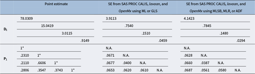
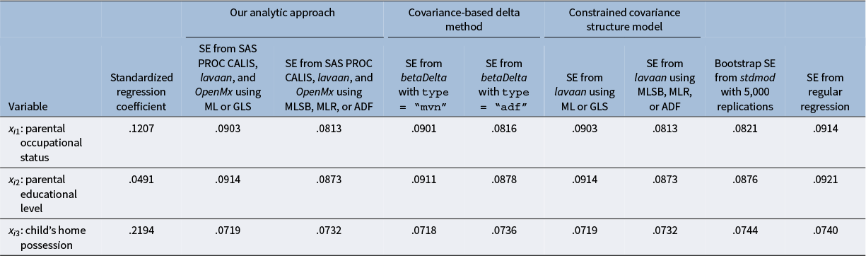
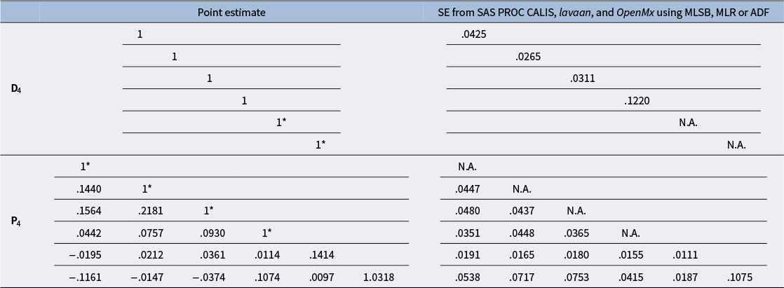
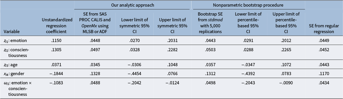
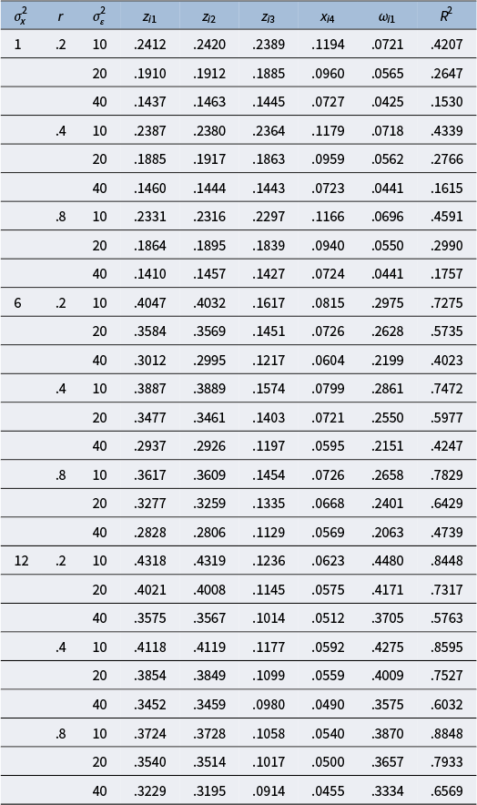


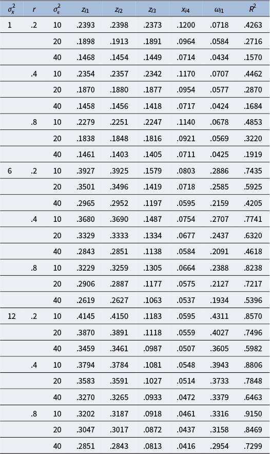


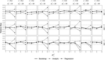


 Open access