


1. Introduction
The advancement and retreat of Antarctic sea ice is the largest annually recurring event on Earth (Massom and Stammerjohn, Reference Massom and Stammerjohn2010), and a significant portion of its natural variability appears to be associated with synoptic variability (Uotila and others, Reference Uotila2011; Vichi and others, Reference Vichi2019). However, our current understanding of these interactions is still incomplete, especially the effects of passing cyclones on the marginal ice zone (MIZ; Vichi and others, Reference Vichi2019). The MIZ is a highly dynamic and complex region of the (partially) ice-covered ocean, where the interactions between the ocean and atmosphere are stronger and more variable, and where weather conditions such as polar cyclones produce the most rapid and often extreme changes of these interactions (Andreas and others, Reference Andreas2010; Zhang and others, Reference Zhang, Schweiger, Steele and Stern2015; Vichi and others, Reference Vichi2019; Alberello and others, Reference Alberello2019). The evolution of the Antarctic MIZ, and also the emerging Arctic MIZ (Wadhams and others, Reference Wadhams, Aulicino, Parmiggiani, Persson and Holt2018), is characterised and governed by the dynamics and thermodynamics of frazil and pancake ice (Doble and others, Reference Doble, Coon and Wadhams2003; Doble and Wadhams, Reference Doble and Wadhams2006) – small, circular and mobile ice floes that form during turbulent ocean conditions at the outer regions of the ice cover. This outer region is conventionally between 5 and 100 km wide (Feltham, Reference Feltham2005; Heorton and others, Reference Heorton, Feltham and Hunt2014), and is usually defined as the area of the ocean covered by 15–80% sea-ice concentration (SIC; Strong and others, Reference Strong, Foster, Cherkaev, Eisenman and Golden2017; Rolph and others, Reference Rolph, Feltham and Schröder2020). The use of the concentration-based definition is a conventional operational choice derived from Arctic consideration, which may be less suitable in the Antarctic (Vichi, Reference Vichi2021, and references therein). Its application to the Antarctic MIZ is subject to the limited validation of remote-sensing products by in situ observations. Very little field data of metocean (meteorological and oceanographic) conditions are available in the Southern Ocean and even less in the MIZ (Derkani and others, Reference Derkani2020). Therefore, although the operational definition is applicable in the Arctic, where there is a good agreement between the ice type and ice cover, it is less reliable in the Southern Ocean, where the ice type is less related to the concentration value (Vichi, Reference Vichi2021). This study is therefore not based on a fixed definition of the MIZ, as constrained by concentration thresholds, but it rather considers the Antarctic MIZ extent based on the region of young and/or fractured sea ice that is continuously affected by atmosphere–ocean interactions, in the form of heat and momentum exchanges, wind and ocean current drag, and wave–ice interactions (Kohout and others, Reference Kohout, Williams, Dean and Meylan2014; Zhang and others, Reference Zhang, Schweiger, Steele and Stern2015; Vichi, Reference Vichi2021).
Sea ice moves as a consequence of external forces – atmospheric and oceanic forcing – and internal ice stresses but the principal factor being the wind forcing (Vihma and others, Reference Vihma, Launiainen and Uotila1996). Storm-induced waves are generated close to the ice edge, and can propagate hundreds of kilometres into the ice cover, leaving behind a wake of less consolidated freezing floes (Squire, Reference Squire2007; Kohout and others, Reference Kohout, Williams, Dean and Meylan2014). This has been suggested to delay the consolidation of the ice cover and maintain the mixed frazil-pancake field (Vichi and others, Reference Vichi2019), causing the ice cover to become more susceptible to winds and underlying currents (Dumont and others, Reference Dumont, Kohout and Bertino2011; Kohout and others, Reference Kohout, Williams, Dean and Meylan2014). Winds transfer momentum to the ice cover, and under free-drift conditions, i.e. the absence of internal stresses, the sea ice changes from moving to the left of isobars (Southern Hemisphere) to moving almost parallel to the isobars, with a linear relationship to the surface wind velocities (Wassermann and others, Reference Wassermann, Schmitt, Kottmeier and Simmonds2006). This ratio between the ice drift speed and wind speed is known as the wind factor and is a key determinant for the dynamics of sea ice (Nakayama and others, Reference Nakayama, Ohshima and Fukamachi2012), with the angle between the drift vectors being the turning angle (Doble and Wadhams, Reference Doble and Wadhams2006). The general rule-of-thumb states that the wind factor is 2% for pack ice (Leppäranta, Reference Leppäranta2011), however higher values have been reported for pancake ice conditions, both in the Arctic (Lund and others, Reference Lund2018) and the Antarctic (Doble and Wadhams, Reference Doble and Wadhams2006).
Sea ice, simultaneously with the ocean, responds to the atmospheric forcing at both the synoptic (multi-day) and inertial (sub-daily) frequencies (Heil and others, Reference Heil, Massom, Allison, Worby and Lytle2009). Wind forcing events such as the passing of polar cyclones may resonantly force inertial oscillations of sea ice on the left (Southern Hemisphere) of their track (Lammert and others, Reference Lammert, Brümmer and Kaleschke2009). Therefore, drift trajectories often include circular or elliptical loops – the inertial oscillations – superimposed on an approximately steady translation (McPhee, Reference McPhee1988). This inertial response of sea ice has been reported for both the Arctic (Lammert and others, Reference Lammert, Brümmer and Kaleschke2009; Gimbert and others, Reference Gimbert, Marsan, Weiss, Jourdain and Barnier2012) and the Antarctic (Doble and Wadhams, Reference Doble and Wadhams2006; Heil and others, Reference Heil, Massom, Allison, Worby and Lytle2009; Alberello and others, Reference Alberello2020). In free-drift conditions or when sea ice is broken, the ice floe is expected to oscillate as an oceanic fluid parcel. However, the friction between the bottom of the ice and the ocean surface or internal stresses caused by mechanical interactions within the sea-ice cover may cause the inertial oscillations to dampen within a few days (Gimbert and others, Reference Gimbert, Marsan, Weiss, Jourdain and Barnier2012).
In this paper, we showcase one of the longest ice buoy trajectories that never left the Antarctic MIZ, as it drifted for 4 months from the South Atlantic sector to the Indian Ocean sector of the Southern Ocean, under the influence of several synoptic cyclones. We correlate the in situ drift measurements with atmospheric and oceanic reanalysis data, and quantify the impact of wind forcing on ice drift, through the direct transfer of momentum and initiation of inertial oscillations of the sea ice. This analysis highlights the effects that polar cyclones have on ice drift and the wider Antarctic MIZ.
2. Methods
2.1 Field measurements and post processing
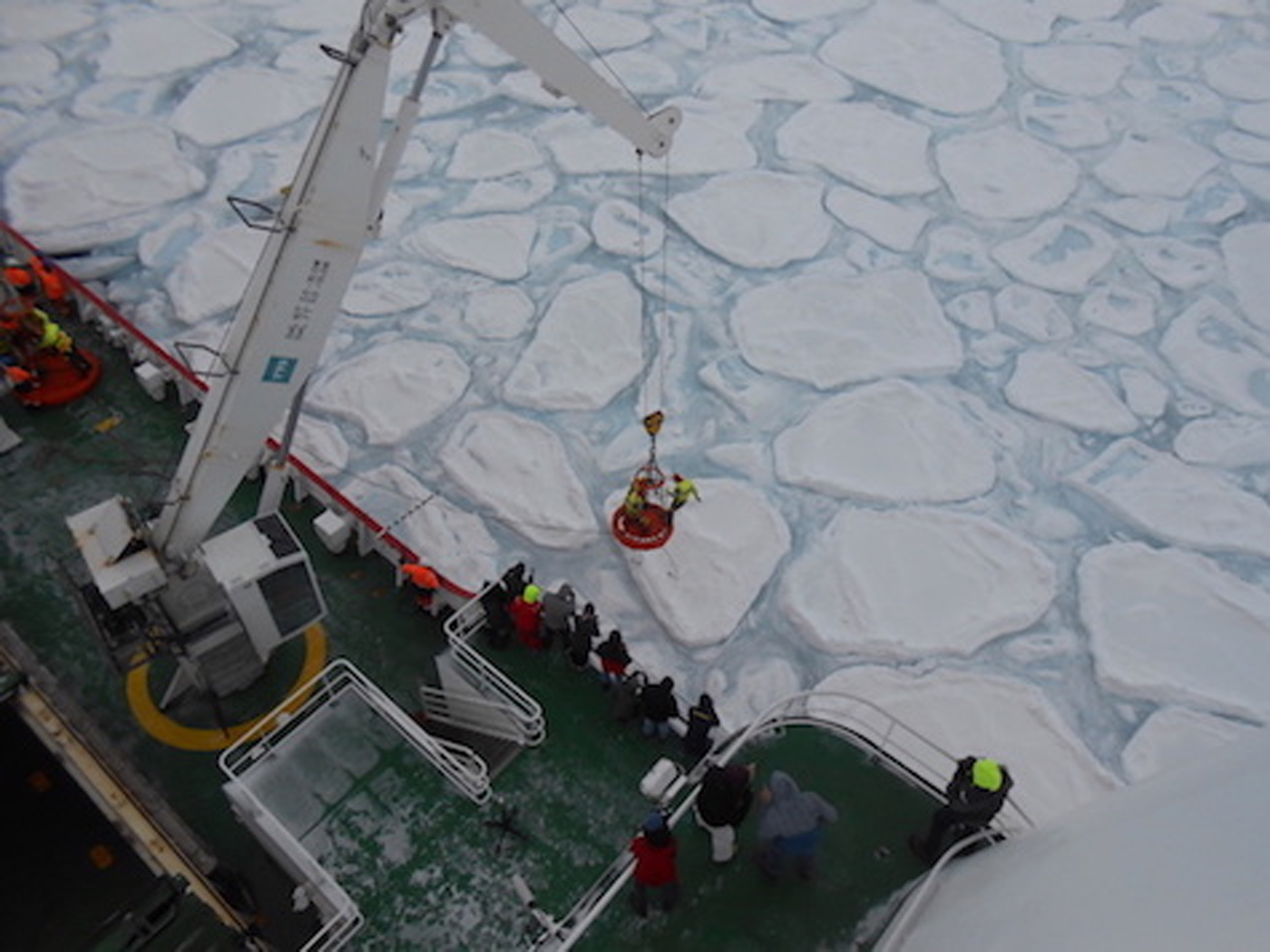
On 5 July 2017, a Trident Sensors Helix Beacon was deployed on a pancake ice floe ≈3 m in diameter (Fig. 1) at 62.8°S and 30.2°E from the SA Agulhas II as one of five buoys deployed within the MIZ (Machutchon and others, Reference Machutchon2019; Eayrs and others, Reference Eayrs2019b), ≈100 km from the northward ice edge. The buoy was a non-floating device which transmitted its GPS position data at a sampling frequency of 4 h through the Iridium system until its signal was lost on 1 December 2017 at 61.5°S and 55.0°E, due to ice melting. The other four buoys only transmitted information until around 20 July 2017, and have been previously analysed by Vichi and others (Reference Vichi2019) and Alberello and others (Reference Alberello2020), over this shorter timeframe.
The ice conditions and deployment of the buoy on a pancake floe using the ship crane. The diameter of the basket is 1.5 m.
The buoy's longitude and latitude positions were used to derive its zonal and meridional velocity components using the linear approximation:


where Δx and Δy are the zonal and meridional geodesic distances travelled between consecutive points along the buoy's trajectory, and Δt is the time interval (4 h). The error estimation of the ice-drift velocity can be attributed to two sources, the first being the tracking error between two consecutive GPS points. However, when displacements (Δx and Δy) are retrieved from drifting buoys, the tracking error (${\rm \sigma }_{{\rm tr}}^2$ ) is 0, since buoys remain fixed relative to the ice floe of deployment (Dierking and others, Reference Dierking, Stern and Hutchings2020). Secondly, there may be errors in the GPS location of the buoy – the geolocation error (Lindsay and Stern, Reference Lindsay and Stern2003). The calculation of the displacements is prone to the errors of the coordinate readings, making its uncertainty ${\rm \sigma }_{\rm d}^2 = 2{\rm \sigma }_{{\rm coord}}^2$
 (Dierking and others, Reference Dierking, Stern and Hutchings2020). However, as seen in Figure 2, the buoy drifted with minimal latitudinal change (<2°) and therefore we may assume identical geolocation errors, which would cancel out when calculating the drift velocity. The major uncertainty of the buoy's velocity would be rather due to the timing of the GPS locations; however, Hutchings and Hibler (Reference Hutchings and Hibler2008) found that velocity errors are <10% for sampling intervals >1 h.
The full trajectory of the buoy (time gradient trajectory from light blue to dark blue) from 5 July to 1 December 2017. The shadings show the AMSR2 SIC with values between 0 and 100% on 1 December. The green circle denotes the end of the ice extent advance season on 30 September. The red circle denotes the beginning of the melt season on 1 November. The green line indicates the ice edge at 0% ice concentration for 30 September, the maximum northward extent of sea ice. The three red boxes indicate the three loops within the buoy's trajectory.

The meander coefficient acts as a primary quantitative measure for the kinematics of sea-ice drift (Vihma and others, Reference Vihma, Launiainen and Uotila1996). As ice drifts under the influence of erratic winds, ice floes change direction and deflect from their primary drift direction. This results in their drift trajectories exceeding the geodesic distance between two points. The ratio between these two distances is called the meander coefficient and is calculated as:

where ΔD is the geodesic displacement between the start and end points of the experiment and I is the total cumulative trajectory length, determined by the four-hourly positions of the buoy, for the 4-month period. We computed this as a time series for each four-hourly position of the buoy, showing the progressive meander coefficient as the time window increased. We then additionally computed two discrete meander coefficients over constant intervals of 1 and 5 d for the full trajectory of the buoy in order to analyse how the passing cyclones affected its drift and its seasonal variation. A greater meander coefficient signifies a more erratic trajectory, whereas a value of M = 1 indicates that the buoy travelled in a straight line. It must be noted that although the meander coefficient is a ratio between two distances, it is also a function of time, as it is dependent on the sampling intervals of the buoy's positions and its deployment duration (Heil and others, Reference Heil, Massom, Allison, Worby and Lytle2009), as it will be presented in Section. 3.3.
Additionally, the framework developed by Lukovich and others (Reference Lukovich, Geiger and Barber2017) is used to assess the directional changes of the buoy's drift path in response to the atmospheric forcing, estimated by ERA5 reanalyses. The framework is based on Lagrangian statistical analyses using particle dispersion theory which shows us whether ice drift is in a sub-diffusive, diffusive, ballistic or super-diffusive dynamical regime using single-particle (absolute) dispersion statistics (Lukovich and other, Reference Lukovich, Geiger and Barber2017). A number of prior studies exist using Lagrangian dispersion and ice-buoy trajectories to quantify sea-ice drift and deformation in the Arctic (e.g. Rampal and others, Reference Rampal, Weiss, Marsan, Lindsay and Stern2008, Reference Rampal, Weiss and Marsan2009); however, it has not been considered to our knowledge in the Antarctic.
Single-particle (absolute) dispersion provides a signature of circulation and organised structure in the flow field, and also shows the linear time dependence in fluctuating velocity variance characteristic of turbulent diffusion theory (Taylor, Reference Taylor1922; Rampal and others, Reference Rampal, Weiss and Marsan2009). It is defined as (Taylor, Reference Taylor1922):

where x i is the zonal and meridional position of the ith particle in the ensemble as a function of the passed time, t, and where the angular brackets denote the ensemble mean. However, as this analysis is based on only one buoy, the ensemble mean could not be computed as multiple buoys would be needed. Therefore, the ergodic assumption was applied, which allowed us to calculate the absolute dispersion of the buoy in time instead of space.
Drift dynamics are characterised by the scaling exponent β (the slope between the single-particle dispersion of sea-ice drift and the elapsed time) according to the relation:

where β > 1 relates to a super-diffusive dynamic regime, β = 1 to a diffusive regime and β < 1 to a sub-diffusive or ‘trapping’ regime (Lukovich and others, Reference Lukovich, Geiger and Barber2017). A super-diffusive regime captures long-range correlations and organised structure in the sea-ice drift field that is unrestricted by diffusive energy losses, for example, through ice mechanics (Lukovich and others, Reference Lukovich, Geiger and Barber2017). A diffusive regime describes the behaviour of buoys/ice floes that follow independent random walks, while a sub-diffusive regime denotes the trapping that would occur with dominating contributions from ice–ice interactions (Lukovich and others, Reference Lukovich, Geiger and Barber2017). In this study, we compare the scaling exponent of the total absolute dispersion during the periods of high meandering to the overall scaling exponent to identify transitions between the dynamical regimes and the effect that atmospheric forcing has on ice drift.
2.2 Environmental conditions
Environmental conditions were obtained from satellite data and reanalysis products for the full duration of the buoy's drift. The daily SIC as well as sea-ice extent (SIE) were obtained from remote sensing, acquired from the passive microwave Advanced Microwave Scanning Radiometer 2 (AMSR2) sensor at a 3.125 km horizontal spatial resolution and a daily frequency (Spreen and others, Reference Spreen, Kaleschke and Heygster2008). This was complemented by the lower resolution Special Sensor Microwave Imager/Sounder (SSMIS) product, which produces SIC with a spatial resolution of 25 km. SIC isolines are used in this analysis as subjective reference values to be considered in relation to the buoy location and drift conditions. Given that there are known differences between the products of the order of 10% during winter and spring (Beitsch and others, Reference Beitsch, Kern and Kaleschke2015) and the known limitations of using a fixed threshold (Kern and others, Reference Kern2019), we consider SIC reference values from >0 to 80%. We will refer to the 0% isoline as the ice edge, although this region is acknowledged to be heterogeneous and fragmented. Results are only marginally affected by considering the standard 15% value, with a maximum deviation of ~50 km, which is still in the range of differences between satellite products. We also note that using the 15% SIC contour would lead to an early melt that was not recorded by the Trident buoy, which is a non-floating device.
The most southerly >0% ice concentrations were determined for each longitude within the defined sample region and calculated for each day within the 4-month drift. The distance between the buoy and the sea-ice edge was thereafter calculated as the meridional geodesic distance between the two latitudes, along the same longitude, for each day of the buoy's drift. Following this, the meridional drift velocity of the ice edge was additionally computed as the change in the daily ice edge latitudinal positions for the same longitude as the buoy. This was calculated using the following equation:

where V w is the average daily meridional change of the ice edge in m s−1, n is the time index of the discretized series of the ice edge latitudes, Δy is the length of one degree latitude in m and Δt is the time interval in seconds.
ERA5 reanalysis was used to obtain synoptic scale meteorological and oceanic conditions – the surface wind velocities (at 10 m), the mean sea level pressure, the air temperature (at 2 m) and the significant wave height (up to 15% ice concentration) – given at an hourly frequency and with a 0.25 × 0.25 degrees horizontal spatial resolution. The validation of the reanalysed atmospheric variables in the Southern Ocean against the ones measured along the cruise track for the duration of the expedition is available in Vichi and others (Reference Vichi2019).
2.2.1 Synoptic cyclones identification
The South Atlantic sector of the Southern Ocean, and particularly the eastern Weddell Sea, is a region of net cyclolysis for cyclones developing near South America and other regions of open ocean genesis (Hoskins and Hodges, Reference Hoskins and Hodges2005; Yuan and others, Reference Yuan, Patoux and Li2009; Vichi and others, Reference Vichi2019). Majority of severe cyclones occur in winter in the Atlantic at ~0°, 30° and 90°E, with good agreement among several storm tracking methods (Grieger and others, Reference Grieger, Leckebusch, Raible, Rudeva and Simmonds2018). These cyclones, with diameters ranging between 500 and 2000 km (Hoskins and Hodges, Reference Hoskins and Hodges2005; Uotila and others, Reference Uotila2011), are associated with strong winds, and are vehicles of moisture and heat to the high latitudes (Woods and Caballero, Reference Woods and Caballero2016; Messori and others, Reference Messori, Woods and Caballero2017), which in turn greatly affect the thermodynamics and dynamics of sea ice in this region.
The buoy exhibited many loops and meanders (Fig. 3) as it drifted under the influence of winds during cyclone activity. As polar cyclones have a typical frequency of one occurrence every 5–7 d (Hoskins and Hodges, Reference Hoskins and Hodges2005; Vichi and others, Reference Vichi2019; references cited in the manuscript), and because of the relatively short period and confined trajectory of the buoy, they can be tracked without the need of automatic tracking algorithms. Therefore, to investigate the impacts that the cyclones have on ice drift, we applied a visual inspection method of the ERA5 mslp and 2 m temperature fields at four-hourly intervals, for the 4-month drift of the buoy. Wei and others (Reference Wei and Qin2016) reported that the average intensity for cyclones in the Southern Ocean, between 1979 and 2013, was 968.4 hPa in spring, 972.4 hPa in summer, 968.7 hPa in autumn and 967.4 hPa in winter. Therefore, for this study, we only considered cyclones with core pressures <970 hPa, as the buoy did not drift during austral summer. Ten cyclones were therefore identified by low-pressure troughs <1000 km from the buoy, and by an increase in air temperature to near melting point close to the ice edge, on the eastern flank of the cyclone (Vichi and others, Reference Vichi2019). Once the cyclones were identified, the dates when the cyclones were closest to the buoy were calculated using a nearest neighbour method and then related to the loops and meanders in the buoy's trajectory. A time series of the mslp in the vicinity of the buoy, as well as maps of the mslp and 2 m temperature fields for when these cyclones were closest to the buoy, overlaid with trajectories of the cyclones from 12 h before to 12 h after each cyclone was closest to the buoy, can be found in Appendix A Figures 14 and 15, respectively. This analysis, however, does not include the analysis of the first 20 d of data which has been analysed by Vichi and others (Reference Vichi2019) and Alberello and others (Reference Alberello2020).
Three case studies of large loops in the drift trajectory of the buoy for (a, b) 9–20 August; (c, d) 26 September–12 October; (e, f) 21–31 October. The gradient blue lines in the left column are colour correlated to the time gradient colour in Figure 2, and denote the buoy's trajectory, moving from left to right. The shadings show the AMSR2 sea-ice concentration between 0 and 100% on the last day for each corresponding meander. The dark-blue points in the right column panels denote the position of the buoy at 12:00 h every day, for ~10 d; the light-blue points show when each cyclone was closest to the buoy using the labels from Table 1.

2.2.2 Estimated significant wave height
The buoy did not measure ocean waves, but waves-in-ice are available for the first 16 d of the deployment through other instruments. As it will be demonstrated in the Results section, the buoy never left the MIZ and free-drift conditions. Therefore, we assume that there were no major changes in ice conditions from the observed conditions during deployment, and hence waves-in-ice conditions measured during this initial period can be considered representative of the MIZ. In order to estimate the significant wave height (H S) at the buoy's location, the coefficient of wave attenuation was first estimated, using the modelled ERA5 wave fields at the sea-ice edge and a 16 d time series of H S measured by the Waves In Ice Observation System (WIIOS; Eayrs and others, Reference Eayrs2019b). This WIIOS, analysed by Alberello and others (Reference Alberello2020) (buoy B2), was deployed ≈12 h prior to the Trident Sensors Helix Beacon's deployment in the MIZ and followed a very similar drift path, which can be seen in the Appendix B Figure 16. This allowed for the assumption that the waves-in-ice activity was the same for both buoys during the first 16 d of deployment.
In this simple approximation, the modelled ERA5 wave energy in the ocean at the sea-ice edge is assumed to decay exponentially to the location of the WIIOS (Kohout and others, Reference Kohout2020), and to travel meridionally south along the same longitude. A time series of the wave attenuation was calculated using the following equation:

where DY is the geodesic latitudinal distance in metres, H Sw is the ERA5 modelled H S at the 0% SIC sea-ice edge for the same longitude as the WIIOS, and H Si is the H S measured by the WIIOS. As explained in Section 2.2, our results are only marginally affected by the SIC threshold used in this study and therefore there is little sensitivity to this choice of the >0% sea-ice edge in the incident wave field. The resulting coefficient and its distribution are shown in Figure 4. The median of this time series was then determined to be α = 5.17 × 10⁻⁶ m−1, with an error (shaded region in Fig. 4a) calculated through the error propagation formula:

where stdDY is the std dev. of the latitudinal distance in meters. However, as the median was biased towards the initial period of high waves affected by the extremes (Vichi and others, Reference Vichi2019) we removed the first 25th percentile of the time series and once again calculated the median, which was then determined to be α = 6.12 × 10⁻⁶ m−1 (also shown in Fig. 4b). For comparison, Kohout and others (Reference Kohout2020) reported attenuation coefficient ranges of α = 1.6–5.0 × 10⁻⁶ m−1 in low SIC (≤80%) and α = 26.5–32.7 × 10⁻⁶ m−1 in high SICs (>80%), in the Ross Sea. The higher estimated attenuation coefficient was then used to compute the H S time series (H Si) in sea ice at the buoy's location for its full 4-month drift. This was calculated using the following equation:

where H Sw is the re-analysed ERA5 H S in the ocean at the sea-ice edge for the same longitude as the buoy.
(a) The time series of the attenuation distance and its error propagation shaded in blue for the WIIOS from 4–19 July 2017 and (b) its corresponding distribution (blue) and the distribution when the 25th percentile is removed (orange). Both corresponding medians are denoted.

We acknowledge the limitations of calculating the wave attenuation and the significant wave height within the sea-ice cover using this approach, as one needs to consider the temporal and spatial variability of direction, ice conditions, ice extent, wave event duration and wave speed (Kohout and others, Reference Kohout2020). This estimate is therefore an approximated method to consider the role of waves throughout the buoy's drift, and the possible relationship between waves, ice and passing cyclones.
2.2.3 Correlation between buoy drift and wind forcing
The wind factor F and turning angle θ were estimated using the least squares regression method from Kimura and Wakatsuchi (Reference Kimura and Wakatsuchi2000). This calculation used the time series of wind and sea-ice drift, neglecting the temporal variation of the ocean current beneath the ice cover, due to the lack of ocean current observations (Nakayama and others, Reference Nakayama, Ohshima and Fukamachi2012). In this case, the wind factor and turning angle subsequently absorb the influence of the ocean current.
The variables U w, V w, and u i, v i denote the zonal and meridional components of wind and ice, respectively. The index of the discretised series of wind and ice drift is denoted by k, with n being the upper bound of the summation. These equations can be written as:


where


From here, the vector coefficient of determination $R_{\rm v}^2$ can be calculated using the following equation adopted from Kimura and Wakatsuchi (Reference Kimura and Wakatsuchi2000):

In addition, the Pearson coefficient of determination $R_{{\rm w}, {\rm i}}^2$ was also calculated to determine the linear relationship between the modulus of ice drift and wind:

where ${\mathop{\rm cov}}$ is the covariance, σw is the std dev. of the wind speed and σi is the std dev. of the ice drift.
3 Results: drift measurements and analysis
3.1 The impact of cyclones on sea-ice drift
Over the 4-month drift, the buoy travelled a net transition displacement of ≈1336 km within the Indian Ocean sector of the Southern Ocean, with minimal latitudinal change (<2°) (Fig. 2). During this eastward drift, the buoy's trajectory was characterised by sharp turns and loops, in response to ten cyclones (Table 1) which passed over/near the buoy. These cyclones, although not part of the top 1% of winter cyclones (Wei and Qin, Reference Wei and Qin2016), had minimum pressures within the range of 940–960 hPa and maximum wind speeds between 10 and 21 m s−1, which greatly impacted the buoy's drift (Fig. 3).
Features of the cyclones which occurred during the loops as simulated by ERA5

The left-hand-side of Figure 3 highlights these three large loops superimposed on the AMSR2 SIC for the last day of each corresponding loop, when the buoy was dynamic and mobile at high ice concentrations (>80%). The right-hand-side shows the buoy's trajectory with its daily position at 12.00 h, and its position when each cyclone was closest to it.
The first large cyclonic loop, occurring between 9 and 20 August, was a result of the three polar cyclones A1–A3 (Table 1). The buoy initially travelled south-east during the passage of cyclone A1. Cyclone A2 then caused the buoy to drift north-west before switching north-easterly under the influence of cyclone A3. The second loop along the buoy's trajectory occurred between 26 September and 12 October at ~10° eastward of the previous loop. This tighter loop was a result of the four cyclones B1–B4, which travelled eastwards impacting the sea-ice cover. Cyclone B1 initially caused the buoy to travel in a south-eastwards direction before switching to a north-eastwards direction. The second cyclone (B2) resulted in several changes in the buoy's drift direction; a southerly, westerly and then a north-easterly drift. During the last two cyclones (B3 and B4), the buoy travelled in two small anti-clockwise loops before finally drifting in a south-easterly direction. The final large loop, occurring between 21 and 31 October, was much more elongated. Cyclone C1 caused the buoy to drift in a south-westerly direction, before shifting to a southerly direction. The second cyclone (C2) caused the buoy to drift north-westerly, before switching to a north-easterly direction under the influence of cyclone C3.
3.2 Distance from ice edge
Figure 5 shows the latitudinal extent of the buoy's trajectory and the sea-ice edge from the AMSR2 and the SSMIS sensors, as well as the locations of the 80% isolines which mark the putative extent of the MIZ. The SSMIS ice edge was generally situated further north than the AMSR2 ice edge, except between mid- to late-September when the AMSR2 ice edge peaked at ≈58°S, while the SSMIS ice edge shifted south to ≈59°S. Additionally, the AMSR2 ice edge and 80% isoline is more variable than the one of the SSMIS sensor. The biases between the AMSR2 and SSMIS sensors can be due to the differences in algorithm sensitivity to ice edge conditions and due to the different spatial resolution of the sensors (Kern and others, Reference Kern2019; Meier and Stewart, Reference Meier and Stewart2019).
Latitudinal location of the buoy (green line) and the ice edge, defined as the >0% sea-ice concentration contour, along the same longitude, for each day of the buoy's trajectory. The dark blue and light blue lines denote the latitude of the AMSR2 ice edge and 80% contour, respectively. The red and pink lines are from the SSMIS sea-ice product. The red star symbols indicate the time when the storm cores were closest to the buoy's location, clustered in the three sets listed in Table 1. The green box denotes the five storms previously examined by Vichi and others (Reference Vichi2019) and Alberello and others (Reference Alberello2020). The right axis is scaled to show the relative distance of each line from the initial point of deployment.

Despite the difference in the sensors, the buoy was always south of the 80% ice concentrations, only drifting into lower SICs in mid-November after the melt season began. However, according to the AMSR2 sensor, the buoy left the ice cover on 29 November – 2 d before the buoy stopped transmitting. This discrepancy is likely due to an underestimation of the low ice concentrations by the satellite product. This can be attributed to the limited capability of the AMSR2 sensor in detecting thin ice near the ice edge, particularly during the melt season (Liu and others, Reference Liu, Helfrich, Meier and Dworak2020). This caused the sea ice to be interpreted by the high-resolution ASI algorithm as ocean. There are inherent uncertainties with ice concentrations lower than 15% as brash ice, small ice floes or flooding by wave action may cause the ice to be interpreted as open ocean (Meier and others, Reference Meier, Fetterer, Stewart and Helfrich2015; Liu and others, Reference Liu, Helfrich, Meier and Dworak2020).
As the transmission period of the buoy started at the beginning of July, the full asymmetrical seasonal cycle of the Antarctic sea-ice cover is less visible. The ice edge was already quite north in July, therefore only half of the sea-ice advance season is shown. However, the rapid retreat from the beginning of November until the end of the transmission period is more prominent. The buoy's location slowly shifted northward until mid-October. Afterwards, while the ice edge was rapidly retreating for both sensors, the buoy was pushed further northwards (the maximum northward location from the point of deployment was attained in mid-November, see Fig. 5 right axes).
Figure 5 additionally shows the relative distance from the point of deployment (left axis, assuming a geodesic distance along the meridian). This confirms that the buoy was generally over 200 km south of the ice edge, while additionally reaching distances of ≈350 km between September and October, independently of the ice-edge location uncertainty. There was an initial 200 km advance of the ice in less than a month, which was likely due to thermodynamic growth (Doble and Wadhams, Reference Doble and Wadhams2006), causing the freezing front to moving northwards, however the extent of this northwards movement was not followed by the buoy.
3.3 Metocean drivers
Figure 6 compares the meridional velocity components of the sea-ice edge estimated from the AMSR2 SIC and the buoy meridional drift. The ice edge is displaced meridionally during the passage of cyclones (Vichi and others, Reference Vichi2019), which is partly visible in the buoy displacement.
The meridional velocity component of the estimated sea-ice edge (orange) and the buoy (blue). This does not include the last few days when the ice edge started melting (from ≈15 November). The grey horizontal line indicates 0 m s−1. The other graphical elements are as described in Figure 5.

Although the buoy spent most of its drift over 200 km from the ice edge (Fig. 5), where the mobility of ice is assumed to decrease due to consolidation, Figure 6 indicates that the buoy drifted similarly to the ice edge, although with a dampened signal. Figure 7 further shows that the zonal and meridional velocities of the buoy motion varied according to wind forcing. During the periods of frequent cyclone activity, indicated by the four rectangular boxes, the sea-ice velocity notably increased with the wind velocity, while additionally following the direction of the wind's velocity components. The overall drift velocity of the buoy does indicate a high correlation to wind forcing, suggesting minimal if not absent internal stresses of the ice, indicative of ice dynamics being in consistent free drift conditions throughout the trajectory. However, there are a few increases in both the wind and ice drift speeds that do not correspond to the passage of a cyclonic event. Therefore, it is important to quantify the drift response objectively through the analysis of the wind factor and turning angle, which will be done later in this section.
Velocity components of the buoy (on the left axis) and 10 m wind from the ERA5 reanalyses (on the right): (a) zonal component and (b) meridional component. The other graphical elements are as described in Figure 5.

The response of the buoy to the passage of the cyclonic systems is further examined by analysing its meander coefficient (Fig. 8) and absolute dispersion (Fig. 9) as described in Section 2.1. The buoy travelled a total trajectory distance of ≈3322 km with a net transition distance of ≈1336 km resulting in a final meander coefficient of 2.49 at the end of the buoy's 4-month drift (Fig. 8). This conformity of the eastwards drift of the buoy is also highlighted in Figure 9 where the total absolute dispersion is governed by the zonal dispersion. This can be a result of the steering influence of the Antarctic Circumpolar Current (ACC). Similarly, Heil and others (Reference Heil, Massom, Allison, Worby and Lytle2009), using a 37 d buoy array with a half-hourly frequency, reported low meander coefficients (1.3–2.7) near the coast within East Antarctica, and attributed this relatively straight-line ice drift to be governed by the Antarctic Coastal Current (ACoC). In comparison, Heil and others (Reference Heil2008) reported that hourly meander coefficients, derived for the western Weddell Sea over a 26 d interval, were considerably larger and varied from 4.4 over the continental shelf break to 9.7 on the shallow continental shelf. We recognize that the computation of the meander coefficient is affected by the period over which it is computed. We have therefore compared the cumulative meandering coefficient with the daily and 5-daily periods. The latter is consistent with the periodicity of storms in this region (Hoskins and Hodges, Reference Hoskins and Hodges2005). We are therefore mostly interested in the relative changes rather than in the absolute values.
Time series of the meander coefficient (shown only from 5 August just before the first large loop until 1 December which was the last day of transmission). The dark-blue line denotes the progressive meander coefficient, the light-blue line denotes the daily meander coefficient, and the green line denotes the 5 d meander coefficient. The markers are indicative of the time interval. The horizontal grey line at M = 1 denotes straight-line drift. The red star symbols indicate the time when the storm cores were closest to the buoy location. The three red rectangular boxes denote the three sets of cyclones indicated in Table 1.

The absolute (single-particle) dispersion statistics for the buoy, from 5 August just before the first large loop until 1 December which was the last day of transmission, depicting the zonal (orange line), meridional (red line) and total (blue line) dispersion. The three red rectangular boxes denote the three sets of cyclones indicated in Table 1.

The daily meander coefficient increased with the passage of each cyclone, particularly before the fourth (B1) and just after the sixth (B3) cyclones. In comparison, the meander coefficient computed over a 5 d time window rather captured the combined effect of the three groups of cyclones, indicated by the rectangular boxes. These increases in the meander coefficients would be due to the strong winds associated with the cyclones (see Table 1). The rises in the daily meander coefficient contributed to the cumulative meander coefficient, which increased to ⩾3 during the periods of the frequent cyclone activity and caused the three large loops (Fig. 3). However, similar to the velocity of the buoy (Fig. 7), there were days when the daily meander coefficient notably increased during the periods of reduced cyclonic activity. This can be seen by smaller turns and deflections in the buoy's trajectory (Fig. 2), and is consistent with the indication of free drift conditions and a high correlation to wind forcing as explained above. Towards the end of the trajectory as it started nearing the melt season, the daily and 5 d meander coefficients were close to 1, when ACC would have likely become a more dominant steering influence.
These meandering events greatly affected the meridional dispersion (Fig. 9) causing it to notably decrease, when the buoy would have been pushed southwards by winds on the eastern flank of the cyclones. However, the zonal dispersion was not as affected, although there were small decreases during the periods of frequent cyclone activity but it shows an overall gradual increase as the buoy drifted eastwards. Recalling that the scaling exponent β describes sea-ice dynamical regimes, β = 2.77 for the total absolute dispersion of the full drift period, however the total dispersion is only shown from 5 August, before the first large loop, to 1 December. This indicates that, while drifting within >80% SIC, the buoy was characterised predominantly by a super-diffusive regime, denoting organised structure in the flow field. However, during the three groups of cyclones, sea-ice dispersion was rather characterised by a sub-diffusive regime β < 1, which captures interruptions in organised flow due to ice–ice interactions (Lukovich and others, Reference Lukovich, Geiger and Barber2017, Reference Lukovich2021). These interruptions or ‘trapping’ events would have resulted in the three large loops as the ice cover was compressed by the meridional winds and the displacement of the buoy was limited. The increase in the meander coefficient during cyclone activity, along with the transitions between these dynamical regimes indicate an erratic nature of ice drift, suggesting that the drift patterns (in Fig. 3) are significantly related to atmospheric forcing.
To further investigate the physical control of wind forcing on the buoy's drift, the observed drift speed and direction was compared with ERA5 wind vectors, using the least squares regression method detailed in Section 2.2.3. The wind factor for the buoy showcased a range of 1–6% with an overall mean wind factor of 2.73%, and although it is higher than the rule-of-thumb value of 2%, it is lower than the range of 3–3.5% reported by Doble and Wadhams (Reference Doble and Wadhams2006) for pancake ice in the Weddell Sea. This would be due to the steering influence of the ACC on the buoy. The turning angle was small with a mean value of −19.83° and generally large variations between −50° and +50°, which are consistent with Uotila and others (Reference Uotila, Vihma and Launiainen2000) who reported values from −20° to +60° in the Weddell Sea, using buoy positions that were interpolated at three-hourly intervals. These quantitative measures indicate a high wind response of the buoy throughout its 4-month drift.
The relationship between the buoy and the wind vectors is shown in Figure 10 (left), based on the indicators shown in Eqns (10) and (11). The ice drift speeds have been multiplied by 33 so that the 1:1 line represents an ice drift of 3% of the wind speed. The measured drift speeds are dispersed relatively evenly around the 1:1 line, with a Pearson coefficient of determination (Eqn (17)) of $R_{{\rm w}, {\rm i}}^2 = 0.60$ . In comparison, Alberello and others (Reference Alberello2020) and Doble and Wadhams (Reference Doble and Wadhams2006) reported similar but slightly lower values of R 2 = 0.56 and R 2 = 0.5, respectively, for pancake ice conditions in the Antarctic. They, however, did not report the relationship between ice drift and wind direction, shown in Figure 10 (right). Here the majority of the points are closer to the 1:1 line, with the bulk of them sitting just below it, at the lower portion of the −19.83° turning angle line. However, during periods of quiescence when the wind stresses are smaller, larger turning angles may exist, which could have resulted in a decreased Pearson coefficient of determination to $R_{{\rm w}, {\rm i}}^2 = 0.40$
 .
.
Scatterplots (left) of ice drift speed as a function of wind speed and (right) of ice drift direction as a function of wind direction. The black line is the 1:1 line. The green line is the turning angle at −19.83°.

The vector correlation, expressed by the coefficient of determination in Eqn (16), is high with a value of $R_{\rm v}^2 = 0.76$ . This is higher than the Pearson $R_{{\rm w}, {\rm i}}^2$
 for both the speed and direction, and although they cannot be fully compared, it does indicate that the relationship between ice drift and wind vector is significant. This suggests that the wind not only impacted the buoy's speed, through the transfer of momentum, but it additionally impacted the path of the buoy. Both methods confirm the good correlation between ice drift and wind forcing, suggesting that the winds are the primary contributor towards the observed drift of the buoy, even in regions where the eastwards-flowing ACC is expected to have a greater control.
Intense polar cyclones have been linked to wave propagation through the ice-covered ocean (Vichi and others, Reference Vichi2019). Since the drifting regime of the buoy was highly correlated to atmospheric variability and did not show major seasonal changes during the trajectory, we have used the methods described in Section 2.2.2 to estimate H S at the buoy location assuming a constant ice type over the period. Figure 11 illustrates the timing of the storm-generated waves in the open ocean from the ERA5 reanalyses and the estimates of in-ice waves at the buoy location using the mean attenuation coefficient derived from ice conditions at the time of deployment. The reconstructed attenuation coefficient during the measured period (green box) leads to wave heights that are comparable with the observed peak intensity, but overestimates the background value, which is indicative of changes in the ice conditions between the storms. It is therefore likely that the estimated H S at the buoy location is also overestimated in terms of the background. For reference, we also show the attenuation rates from Kohout and others (Reference Kohout2020) for ⩽80 and >80% SIC (see Section 2.2.2). The buoy drifted mostly in >80% SIC, while the estimated H S (blue line) appears to be more similar to the H S range for ⩽80% SIC, rather than the >80% SIC range where the H S dissipates completely also during the wave observation period in the green box. We thus infer that during storm periods, when the buoy drift was not dissimilar from the one measured during the wave observation period, it is possible that some wave energy may have penetrated at distances ≈350 km from the ice edge.
Time series of (a) the modelled H S at the ice edge from ERA5 (orange line) and (b) the estimated H S at the buoy's position for the 4-month drift period (blue line). The measured H S of the WIIOS for the first 16 d of the buoy's drift is denoted by the green line. The blue and orange shaded areas denote the H S of the buoy calculated using the attenuation coefficient ranges from Kohout and others (Reference Kohout2020) for ice concentrations ⩽80% and >80%, respectively. All the other graphical elements are as in Figure 5.

3.4 Spectral analysis
A power spectral analysis was computed for the velocity components of the buoy to further examine how sea ice responds to wind forcing at both the multi-day and sub-daily (inertial) frequencies. Figure 12 shows the power spectral density (PSD) for the 4-month drift of the buoy and the ERA5 wind velocity components. The wind velocity shows a classical, continuous energy cascade from the lower (multi-day) frequencies to the higher (sub-daily) frequencies. The ice drift velocity is also subject to a similar energy cascade. However, it indicates a clear energy peak at a frequency just below 2 cycles d−1, at 13.47 h, as determined by Alberello and others (Reference Alberello2020) for the first 2 weeks of deployment. The period of these oscillations falls within the theoretical inertial range of 13.47–13.72 h between 61°S and 62°S. As the buoy was deployed and operated in the deep Southern Ocean away from the continental shelf, we did not include the role of tidal forcing that is known to be negligible in off-shelf buoy deployments (Heil and others, Reference Heil, Massom, Allison, Worby and Lytle2009; Lei and others, Reference Lei2021). Tides are effective drivers of sea-ice dynamics in coastal polynyas and close to ice shelves, where they may affect the melting rates (e.g. Hausmann and others, Reference Hausmann2020). In addition, the buoy trajectory was close to an amphidromic point (Kamphuis, Reference Kamphuis2020: Fig. 7.5), where the tidal fluctuation is notably small (between 20 and 60 cm at most).
Power spectral density corresponding to the (left) zonal component of ice drift and the (right) meridional component of ice drift of the buoy for 4 months. The blue line indicates the buoy, and the orange line indicates the ERA5 winds. The light-blue and light-orange shading indicates the 95% confidence intervals for the buoy and ERA5 winds, respectively. The vertical red line indicates the peak associated with inertial oscillations (13.47 h).

A wavelet analysis was additionally performed to yield information about the time series and the frequencies together. To properly isolate the mechanisms that excite inertial oscillations of sea ice in relation to the storm passage, a high-pass Butterworth filter was applied to the buoy's velocity time series in order to filter out the lower frequencies longer than the day. Figure 13 shows the filtered wavelet power spectrum (left) and the filtered wavelet spectrum (right) of both the zonal and meridional velocity components of the buoy. Both components have statistically significant power throughout the time series (being inside the cone of influence), at both the lower and near-inertial, sub-daily frequencies. However, the majority of this power still lies within the lower frequencies despite the use of the high-pass filter. There are three large power intensifications within the lower frequencies (≈128, ≈320 and ≈512 h, corresponding to 5, 13 and 21 d, respectively) for the zonal component, with a weaker and lagged response for the meridional component. These three power maxima occurred between ≈5–20 July (the period analysed by Vichi and others (Reference Vichi2019) and Alberello and others (Reference Alberello2020)), ≈6–26 August and ≈30 September–10 November. The latter two correspond with the dates of the three large loops in Figure 3. This is due to the direct transfer of momentum from the wind forcing, which can be seen in Figure 12 where the sea ice, although with less power, follows the energy cascade of the wind within the lower frequencies.
The wavelet power spectrum (left) and the wavelet spectrum (right) of the filtered spectrum of the buoy for its 4-month drift. The red line indicates the cone of influence, the black contours (left two) and orange dashed line (right two) indicate the 95% significance level. All the other graphical elements are as in Figure 5.

In addition to the synoptic response of the sea ice, the momentum transfer from the winds at the lower frequencies initiated an inertial response, which appears to occupy a well-defined frequency band (see Fig. 13). This is because synchronous with the ocean, sea ice provides a medium that effectively allows the transfer of energy from the lower frequencies (wind forcing) to the semi-diurnal frequencies (Heil and others, Reference Heil, Massom, Allison, Worby and Lytle2009). Therefore, a continuous energy cascade from the lower frequencies of wind velocity is needed to produce both the synoptic and inertial frequency responses in ice drift. A closer visual inspection of Figure 13 suggests that the dates of the strongest inertial oscillations coincided with the dates of the lower-frequency power maxima. More notably, these inertial power maxima additionally coincided with the dates of the three large loops (in Fig. 3); when (1) the ice drift of the buoy changed to be dominated by high-frequency oscillations (Lammert and others, Reference Lammert, Brümmer and Kaleschke2009), and when (2) the rotation velocity was likely greater than the advection velocity (Gimbert and others, Reference Gimbert, Marsan, Weiss, Jourdain and Barnier2012), during ‘trapping’ events captured by the sub-diffusive dynamical regimes (Fig. 9), resulting in the increased meander coefficient (Fig. 8).
Inertial oscillations, although occurring more regularly than the synoptic events at the lower frequencies, are shorter lived and dissipate within a few days (see Fig. 13). This dissipation is expected to be due to kinetic energy dissipation within the Ekman layer, friction occurring between ice floes and the surface ocean (Gimbert and others, Reference Gimbert, Marsan, Weiss, Jourdain and Barnier2012), as well as internal stresses of the ice floes. By means of the outcome of the meandering coefficient (Fig. 8) and the total absolute dispersion (Fig. 9), it is speculated that these forces dampen the rotation, which resulted in a more straight-line trajectory of the buoy, before new oscillations were excited.
4. Discussion and conclusions
The 4-month trajectory from the South Atlantic sector to the Indian Ocean sector of the Southern Ocean was continuously impacted by polar cyclones. Ten of these cyclones were found visually, using methods described in Section 2.2.1, to determine the coupling between the sea ice and atmospheric forcing occurring when polar cyclones pass over the ice edge. The average daily meridional change of the ice edge estimated from the AMSR2 satellite showed large fluctuations (Fig. 6) as it was forced by the passing cyclones as reported previously by Vichi and others (Reference Vichi2019). This indicates that surface winds, particularly the meridional winds associated with polar cyclones, played an important role in reshaping the ice edge (Kwok and others, Reference Kwok, Pang and Kacimi2017; Vichi and others, Reference Vichi2019; Eayrs and others, Reference Eayrs2019a).
While the buoy spent most of its drift over 200 km from the ice edge (Fig. 5), where the mobility of ice is assumed to decrease due to consolidation, the buoy's trajectory showed large meandering and a dynamic response to wind forcing, as it displayed sharp turns and loops while drifting under the influence of the winds (Fig. 3). The final meander coefficient was 2.49, indicating a more straight-line trajectory for the buoy's overall drift. However, during periods when the ten cyclones passed near/over the buoy, all methods describing the meander coefficient increased (Fig. 8). Additionally, while the overall scaling exponent (β = 2.77) of the total absolute dispersion showed a super-diffusive regime; during cyclone activity there was a transition to a sub-diffusive (β < 1) regime, characterised by trapping, resulting in the three large loops (Fig. 3). Together, the meander coefficient and the total absolute dispersion indicate a more erratic nature of ice drift during these periods, suggesting that the drift of the buoy was significantly related to wind forcing during the passage of the cyclones. The ice drift speed also notably increased during the passage of the cyclones (see Fig. 7). This strong relationship was confirmed by the high mean wind factor of 2.73%, the small mean turning angle of −19.83° and good linear correlations of 0.60 and 0.40 for the speed and direction, respectively, and 0.76 for the vector correlation. Together, these all indicate that wind forcing had a dominant physical control on the ice floe trajectory throughout the 4 months, from winter to spring. Additionally, along with the high mobility of the buoy, this high wind response suggests that free-drift conditions likely persisted throughout the buoy's drift.
Although the buoy (and the underlying ice movement) revealed a high wind response, it drifted mostly at distances >200 km from the ice edge, while also reaching distances of ≈350 km, between August and September. Additionally, according to both the SSMIS and AMSR2 sensors, the buoy remained in >80% ice concentrations, only drifting into lower concentrations in mid-November after the melt season began (Eayrs and others, Reference Eayrs2019a). During this retreat of the SIE, the buoy was pushed further northwards to its maximum northward location from its point of deployment. This can be attributed to the increased mobility of sea ice during the melt season, where decreases in ice strength and internal stresses lead to more ice deformation, fracturing and increased drift speeds (Tandon and others, Reference Tandon, Kushner, Docquier, Wettstein and Li2018). At the end of the transmission period there was however a discrepancy between the buoy and the AMSR2 sensor, as the satellite product indicated the buoy was outside the ice cover 2 d before the buoy was lost (presumably due to ice melt and hence sinking of the buoy). This has been attributed to the limited capability of the AMSR2 sensor in detecting thin ice near the ice edge during the melt season (Liu and others, Reference Liu, Helfrich, Meier and Dworak2020). In the overall 4 months, the SSMIS and AMSR2 sensors often differed from each other (Fig. 5). This can be due to the algorithms used by the products and/or their different spatial resolutions. Further analyses will therefore need to be done to better assess the ice extent to determine their accuracy, particularly during the melting period when their error grows. Beitsch and others (Reference Beitsch, Kern and Kaleschke2015) determined that the overall best agreement with ship-based observations and satellite-derived ice concentrations was found using the Bootstrap algorithm, which is in agreement with our finding that SSMIS is a better estimator of the ice edge location in spring.
We speculate that the high mobility of the buoy may have been maintained by heterogeneous ice conditions like the ones observed at deployment. The buoy did not measure waves along its trajectory, and by estimating a constant attenuation coefficient obtained from the first 16 d of deployment, we can speculate that wave energy from the edge may have penetrated in regions of apparent full ice coverage from space. This is a coarse approximation, since it assumes that wave direction, ice conditions, ice extent, wave event duration and wave speed are represented by the conditions observed during the period of direct observations in early July. However, this simple parameterization of wave attenuation suggests that with the high wind response observed, sea-ice conditions during peaks of wave energy in the open ocean may have mechanical properties similar to the pancake-frazil conditions observed during the buoy's deployment, even when the satellite products indicated >80% ice concentrations.
A spectral analysis was done to further elucidate the influence of wind forcing on ice drift. Our results demonstrate that the PSD of both the wind and the ice drift velocity components exhibited a continuous energy cascade (Fig. 12), with majority of their power found within the lower frequencies and a clear energy peak in the inertial range. As the intense polar cyclones passed over/near the buoy, their strong winds excited inertial oscillations of the ice, since ice is embedded within the surface of the ocean (Heil and others, Reference Heil, Massom, Allison, Worby and Lytle2009). The use of a filtered wavelet power spectrum highlighted the response of the buoy to atmospheric forcing at both the lower (synoptic) and inertial frequencies (Fig. 13). It showed three large power intensifications at the synoptic scales of 5, 13 and 21 d for the zonal component, with a lagged response in the meridional component. These power maxima coincided with the three groups of cyclones detected in the atmospheric reanalyses (Table 1). This suggests that there was a direct transfer of momentum from the winds to the sea ice at these scales, although further analysis involving ad hoc numerical models will be required in the future.
The analysis revealed that in addition to the synoptic response of the buoy, there is a plausible correlation between the onset of inertial oscillations and the presence of polar cyclones. The most intense inertial responses occurred during the periods of frequent cyclone activity. This relationship cannot be fully demonstrated because sometimes the power at the inertial frequency was found outside of the dates of higher cyclone activity. Additionally, these power intensifications were often excited before the increase in power at the lower frequencies. The propagation of waves into the ice cover can affect the local drift of ice floes and how they respond to wind and ocean forcing. Therefore, we propose that the penetration of storm-generated waves may be able to help initiate the inertial oscillations observed in the sea-ice drift, allowing the power at the inertial frequency to increase before the power at the lower frequencies. Additionally, as waves helped to maintain the pancake-frazil ice conditions, we speculate that this allows the geostrophic current to keep the weaker inertial oscillations during periods of storm quiescence. Alberello and others (Reference Alberello2020) attributed the strong inertial signature at ≈13 h to the geostrophic current and to full free-drift conditions. It is however unclear how these periods of synoptic events (5–20 d) may drive the initiation of inertial oscillations, as for instance by breaking the consolidated ice into smaller floes (e.g. Gimbert and others, Reference Gimbert, Marsan, Weiss, Jourdain and Barnier2012), or by maintaining a more fluid sea-ice type throughout the extended Antarctic MIZ. The strong influence at the lower (synoptic) frequencies has however been identified as the primary effect of atmospheric forcing and the initiation of inertial oscillations of sea ice has been identified as the secondary effect. The secondary effect greatly influences ice drift at shorter timescales and causes deviations of the ice drift from a straight-line path.
This analysis confirms that the buoy did not leave the Antarctic MIZ throughout its 4-month drift. It also suggests that instead of a local transition from smaller pancake ice floes into a consolidated frozen pack ice (Doble and Wadhams, Reference Doble and Wadhams2006), there is instead a northward push of a frontal band of unconsolidated sea ice. The exact extent of this frontal band and the features of the ice type left behind cannot be inferred from the satellite available data and would require further observational studies.
Based on these observations, the MIZ in this Antarctic sector is much wider than previously thought (see Section 1), even throughout the peak period of the winter sea-ice expansion. The buoy drifted within regions of 80–100% ice concentrations, but the ice was not consolidated as suggested by the high mobility of the buoy. This implies that the concentration-based MIZ definition (see Section 1), where the ice concentration lies between 15 and 80% is inadequate to describe the sea-ice type in the Antarctic MIZ. This is because the highly dynamic nature of the MIZ is maintained despite the high SICs observed from space, due to the complex interactions between sea ice, polar cyclones and storm-generated waves.
Supplementary material
The supplementary material for this article can be found at https://doi.org/10.1017/jog.2022.14.
Acknowledgements
The expedition was funded by the South African National Antarctic Programme (SANAP) through the National Research Foundation (NRF). We thank the captain and the crew of the SA Agulhas II for assistance during the deployment. A.A. and A.T. were funded by the ACE Foundation and Ferring Pharmaceuticals and the Australian Antarctic Science Program (project 4434). A.A. acknowledges support from the Japanese Society for the Promotion of Science (PE19055). A.T. acknowledges support from the Australia Research Council (DP200102828). We thank A. Babanin and Keith MacHutchon for facilitating the purchase and delivery of the Trident Sensors Helix Beacon through the DISI Australia–China Centre Grant ACSRF48199. A.W. thanks J. Rogerson for support with the data processing. We thank L. Fascette for technical support during the cruise.


 Open access