Constraints on mineral formulae used in the calculation of end-members

Given that we have chosen the constituents (i.e. elements) which we will use in the chemical description of a specific mineral grain, there are some very important constraints required by the types of calculations that are described here.

[1] The mineral formulae must be electroneutral.

[2] The sites in the structure of the mineral must be completely occupied by ions and vacancies that are stoichiometrically part of the formula of the mineral.

[3] There must be no excess ions in the formula that cannot be accommodated at the sites in the structure. Thus, for forsterite, (Mg,Fe²⁺)₂SiO₄, Si cannot exceed 1.00 apfu (atoms per formula unit). If a formula has Si = 1.03 apfu, there is nowhere in the crystal structure to put 0.03 apfu Si and hence the chemical formula is physically impossible. An oft-cited example of the effects of non-stoichiometric formulae on calculations involving end-members is given by Rickwood (Reference Rickwood1968), who purportedly showed that calculation of the amounts of end-members for many chemical analyses of garnets is dependent on the sequence in which the simultaneous equations are solved. Hawthorne (Reference Hawthorne2021b) showed that this result was due to the use of chemical formulae that contain the physical errors noted above; in particular, excess amounts of ions which could not be accommodated at the sites in the garnet structure. This situation was noted by Rickwood (Reference Rickwood1968) but overlooked by others citing his paper. An example was given by Deer et al. (Reference Deer, Howie and Zussman1992) and Hawthorne (Reference Hawthorne2021b): a garnet formula of the correct stoichiometry and choice of end-members as components which gives a unique solution for the amounts of component end-members (i.e. the end-members that are linearly independent).

[4] One issue that has not been mentioned in the ongoing debate about end-members is the effect of minor and trace elements. When we consider chemical formulae and the assignment of mineral names, we focus on major and some minor elements and ignore trace elements and minor elements at or below whatever the threshold of detectability of our analytical technique(s), commonly electron microprobe analysis. Some of these trace elements will enter stoichiometrically into the crystal structure of the mineral; others will be adsorbed onto cleavage surfaces and cracks in the mineral; and some will both enter stoichiometrically into the structure and also be partly adsorbed onto cleavage surfaces and cracks. Hence the true number and amounts of these constituents in the mineral will be unknown and too large to be considered rigorously by the methods described here. Thus my attempt at rigour in points (1) to (3) above is doomed to failure: Homo proponit, sed Deus disponit (Thomas à Kempis, 1380–1471). However, if our intent is solely to identify the dominant end-member for a specific analysed mineral, trace elements are present in amounts too low to affect the identity and calculation of the dominant end-member and the issue now comes down to finding the best way to deal with minor elements as comprehensively as possible.

Definitions

Phase: A phase is a chemically homogeneous substance. Most minerals are not chemically homogeneous: they exhibit local differences in occupancy of Wyckoff-equivalent sites that give rise to short-range order (e.g. Hawthorne et al., Reference Hawthorne, Della Ventura and Robert1996, Reference Hawthorne, Della Ventura, Oberti, Robert and Iezzi2005, Reference Hawthorne, Oberti and Martin2006; Hawthorne and Della Ventura, Reference Hawthorne and Della Ventura2007). In order to deal with this issue, I will add the additional requirement that a crystalline phase is chemically homogeneous on a long-range scale. Although this definition exposes our ignorance of where and over what distance ‘short range’ changes to ‘long range’, this ignorance does not materially affect the arguments developed here.

System: A system is a set of entities, in the present case, the set(s) of phases that we will consider. The thermodynamic characteristics possible for a system (isolated, closed, etc.) do not concern us here.

Components: Components are chemically independent constituents of a system (Spear, Reference Spear1993; Anderson, Reference Anderson2005). There are two types of components that depend on the system being considered: system components are needed to describe the total possible chemical variation in that system, and phase components are needed to describe the chemical variability of a specific phase. Here, I will focus on phase components, and let it be understood that when I use the word ‘component’, I will be referring to a phase component unless otherwise stated.

End-member: An end-member is an abstract concept used to identify minerals and a particular mineral species (Hawthorne et al., Reference Hawthorne, Mills, Hatert and Rumsey2021); it is not a mineral [see Nickel (Reference Nickel1995) for the definition of a mineral]. Hawthorne (Reference Hawthorne2002, Reference Hawthorne2021a) has discussed the properties of an end-member: (1) an end-member formula must be irreducible (fixed) within the system considered [i.e. it should not be capable of being factored into components that have the same bond topology (atomic arrangement) as that of the original composition]; (2) it must be compatible with the crystal structure of the associated mineral species, both with regard to stoichiometry and stability of atomic arrangement; (3) it must be electroneutral (i.e. not carry an electric charge). I have heard several comments at scientific meetings that it is not always possible to write a dominant end-member formula for a mineral. This is not so: Hawthorne (Reference Hawthorne2021a) provided a proof that it is always possible to write a dominant end-member formula for a mineral.

One may calculate the proportions of the end-members of a mineral provided that those end-members are linearly independent; i.e. they are phase components of the mineral. If the set of end-members used for such a calculation contains linearly dependent end-members, the linearly dependent end-members are not all phase components and the calculation fails. Removal of the linear dependence converts the set of remaining end-members into phase components of the mineral, irrespective of which linearly dependent end-member is removed. I will refer to such linearly independent end-members as component end-members.

Formula: I refer to Ca₃(Al_1.00Fe³⁺_0.60Cr³⁺_0.40)Si₃O₁₂ as a chemical formula or formula, and (Gr_0.50An_0.30Uv_0.20) as the corresponding end-member proportions.

Aggregate charge of a group: the aggregate charge of the ions in a particular cation group; e.g. for ^X[Ca_2.10Mg_0.80Na_0.10], the aggregate charge of the X-group is 2⁺ × 2.10 + 2⁺ × 0.80 + 1⁺ × 0.10 = 5.9⁺.

Aggregate charges of the groups in a mineral formula: the aggregate charges of the ions in each cation group in a mineral formula; e.g. for ^X[Ca_2.10Mg_0.80Na_0.10] ^Y[Al_1.10Fe³⁺_0.70Ti⁴⁺_0.20] ^Z[Si⁴⁺_2.90Al_0.10]O₁₂, the aggregate charges of the X-, Y- and Z-groups are 5.9⁺ 6.2⁺ 11.9⁺.

Constituent-cation charges of a group: the charges of the individual ions in a particular cation group, e.g. for ^X[Ca_2.10Mg_0.80Na_0.10], the constituent-cation charges of the X-group are ^X[M³⁺₀M²⁺_2.90M¹⁺_0.10].

Constituent-cation charges of the groups in a mineral formula: the charges of the individual ions in each cation group of a mineral formula; e.g. for ^X[Ca_2.10Mg_0.80Na_0.10] ^Y[Al_1.10Fe³⁺_0.70Ti⁴⁺_0.20] ^Z[Si⁴⁺_2.90Al_0.10]O₁₂, the constituent-cation charges of the X-, Y- and Z-groups are ^X[M³⁺_0.00M²⁺_2.90M¹⁺_0.10] ^Y[M²⁺_0.00M³⁺_1.80M⁴⁺_0.20] ^Z[Si⁴⁺_2.90M³⁺_0.10]. I find it more intuitive to use Si⁴⁺ rather than M⁴⁺ for the tetravalent Z-group ions and do so for garnets throughout this paper.

The relationship between chemical formulae, components and end-members

A set S of vectors V is designated a basis (a set of basis vectors) if every element of V may be uniquely written as a finite linear combination of elements of S. The coefficients of this linear combination are components of the vector with respect to S. Thus, we may write the chemical formula of a mineral in terms of its basis vectors and solve the resulting set of simultaneous equations to give the amounts of the components represented by that mineral composition. The solution of such systems of simultaneous equations is governed by the Rouché-Capelli theorem (Shafarevich and Remizov, Reference Shafarevich and Remizov2013; page 58): A system of linear equations with n variables has a solution if and only if the rank of its coefficient matrix A is equal to the rank of its augmented matrix [A|b] where, for the applications described here, [b] is the column matrix involving the stoichiometric amounts of the ions in the mineral formula.

It is straightforward to calculate all the end-members possible for a particular bond topology (crystal-structure arrangement) (Hawthorne, Reference Hawthorne2002, Reference Hawthorne2021a; Gagné and Hawthorne, Reference Gagné and Hawthorne2016). However, the representation of a particular mineral formula in terms of end-members is more complicated. This is shown most effectively using specific mineral examples. Here, I will focus on silicate minerals of the garnet supergroup.

General attributes of the silicate-garnet structure

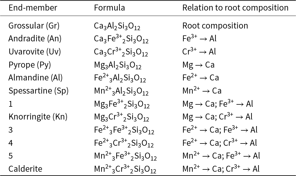
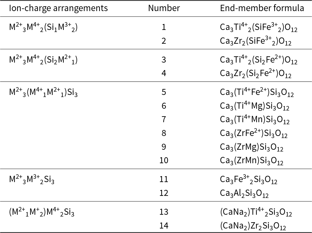
The classification and nomenclature of the garnet-supergroup minerals are described by Grew et al. (Reference Grew, Locock, Mills, Galuskina, Galuskin and Hålenius2013). The general chemical formula of a garnet is generally written as X₃Y₂Z₃O₁₂ where X cations occupy the [8]-coordinated X site, Y cations occupy the [6]-coordinated Y site, and Z cations occupy the [4]-coordinated Z site. Here I will focus initially on garnets of the general formula ^X(Ca,Mg,Fe²⁺,Mn²⁺)₃^Y(Al,Fe³⁺,Cr³⁺)₂^ZSi₃O₁₂. In this system, there is only one arrangement of constituent-cation charges of the groups in the formula (Hawthorne, Reference Hawthorne2002, Reference Hawthorne2021b): ^X2⁺₃ ^Y3⁺₂ ^Z4⁺₃ ^O2^–₁₂. Thus all possible end-member formulae of garnets in this system may be derived by permuting the cations present over the X and Y sites of the structure, and they are listed in Table 1. I will examine whether it is possible to write any garnet formula of the type ^X(Ca,Mg,Fe²⁺,Mn²⁺)₃^Y(Al,Fe³⁺,Cr³⁺)₂^ZSi₃O₁₂ in terms of end-members belonging to the set listed in Table 1, i.e. can we use end-member chemical formulae as components of any garnet formula related to ^X(Ca,Mg,Fe²⁺,Mn²⁺)₃^Y(Al,Fe³⁺,Cr³⁺)₂^ZSi₃O₁₂?

Table 1.

Possible end-member compositions for the general garnet formula (Ca,Mg,Fe²⁺,Mn²⁺)(Al,Fe³⁺,Cr³⁺)Si₃O₁₂

The system grossular–andradite–uvarovite

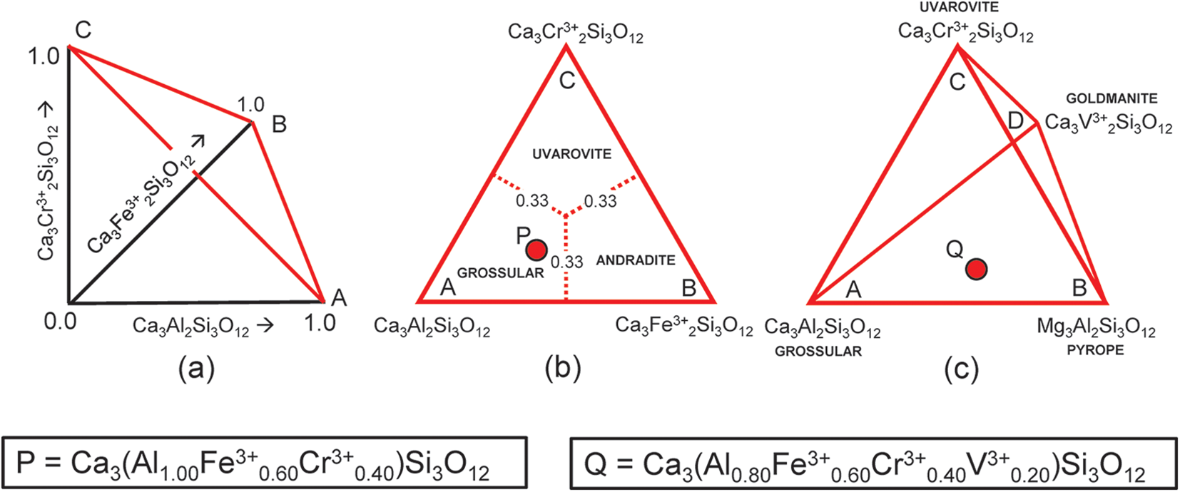
Let us first consider the garnets grossular, andradite and uvarovite. Figure 1a shows variations in amounts of these end-members from 0 to 1 indicated by the arrows, and any garnet composition within this system lies on the red triangle in Fig. 1a, the apices of which are labelled A, B and C. Figure 1b shows the red triangle in the plane of the page with the compositional ranges of each garnet indicated. The end-member Ca₃Al₂Si₃O₁₂ is (arbitrarily) chosen as the origin of the compositional space in Fig. 1b and I will designate it as the origin formula for this representation. Note that the basis vectors of Fig. 1a are linearly independent. However, this is not the case for the end-members of Fig. 1b: if a, b and c denote the amounts of each end-member, respectively, a + b + c = 1. Hence a, b and c are not all components of Fig. 1b; only two of the end-members are components and the amount of the third end-member is given by the requirement that the amounts of the end-members sum to unity, i.e. it is a linear combination of the other two vectors.

Figure 1.

(a,b) Compositional variation in the system Ca₃Al₂Si₃O₁₂–Ca₃Fe³⁺₂Si₃O₁₂–Ca₃Cr³⁺₂Si₃O₁₂; (a) variation in each constituent from 0 to 1; the red triangle denotes the plane in which the three constituents sum to 1; note that the black axes labelled Ca₃Al₂Si₃O₁₂, Ca₃Fe³⁺₂Si₃O₁₂ and Ca₃Cr³⁺₂Si₃O₁₂ in (a) are orthogonal; (b) the red triangle in (a) orientated in the plane of the page; the dotted red lines denote the boundaries between the compositional fields of grossular, andradite and uvarovite; the red circle P marks the formula Ca₃(Al_1.00Fe³⁺_0.60Cr³⁺_0.40)Si₃O₁₂; (c) compositional variation in the system Ca₃Al₂Si₃O₁₂–Ca₃Fe³⁺₂Si₃O₁₂–Ca₃Cr³⁺₂Si₃O₁₂–Ca₃Cr³⁺₂Si₃O₁₂; the red circle Q marks the formula Ca₃(Al_0.80Fe³⁺_0.60Cr³⁺_0.40V³⁺_0.20)Si₃O₁₂.

What happens if we change the origin of composition space to another end-member of the system considered? Nothing changes regarding the end-member proportions as the system is symmetric with regard to the end-members.

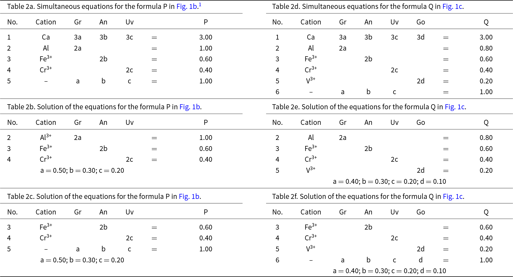
Let P represent the garnet formula Ca₃(Al_1.00Fe³⁺_0.60Cr³⁺_0.40)Si₃O₁₂ in Fig. 1b and let us write the composition P in terms of the end-members and the equation a + b + c = 1 as shown in Table 2a. However, before we try to solve the set of simultaneous equations of Table 2a for the amounts of the component end-members, we must select any set of non-identical equations for which the number of unknowns (3) is equal to the number of equations and solve for the amounts of the component end-members. In Table 2a, equations 1 and 5 are identical and equation 5 is linearly dependent on equations 2, 3 and 4. Two examples are shown in Tables 2b and 2c. Composition P corresponds to Gr_0.50An_0.30Uv_0.20 and is shown as a red circle in Fig. 1b. Is this calculation influenced by the choice of origin formula? No; all choices of an origin in this system are symmetry equivalent and hence the solution is the same, irrespective of the choice of origin.

Table 2.

Simultaneous equations for using the formula in Fig. 1 on the basis of various values of P, Q, a, b, c and d

¹ In each table (here and elsewhere), addition signs are implicit across rows as each row is an equation in a set of simultaneous equations.

The system grossular–andradite–uvarovite–goldmanite

Let us add an additional ion, ^YV³⁺, to the next garnet composition to be considered: Q = Ca₃(Al_0.80Fe³⁺_0.60Cr³⁺_0.40V³⁺_0.20)Si₃O₁₂, shown as the red circle in Fig. 1c. The only possible end-member to represent ^YV³⁺ for formula Q is goldmanite: Ca₃V³⁺₂Si₃O₁₂. As d, the amount of Ca₃V³⁺₂Si₃O₁₂, is linearly independent of a, b and c (except for the constraint a + b + c + d = 1), the end-members occupy the vertices of a tetrahedron in garnet compositional space (Fig. 1c). Table 2d shows the simultaneous equations for composition Q. However, equations 1 and 6 in Table 2d are identical (and hence not linearly independent), and equation 6 is linearly dependent on equations 2 to 5. Any four linearly independent equations can be used to solve for the amounts of the component end-members; two examples are shown in Tables 2e and 2f.

The system grossular–pyrope–uvarovite

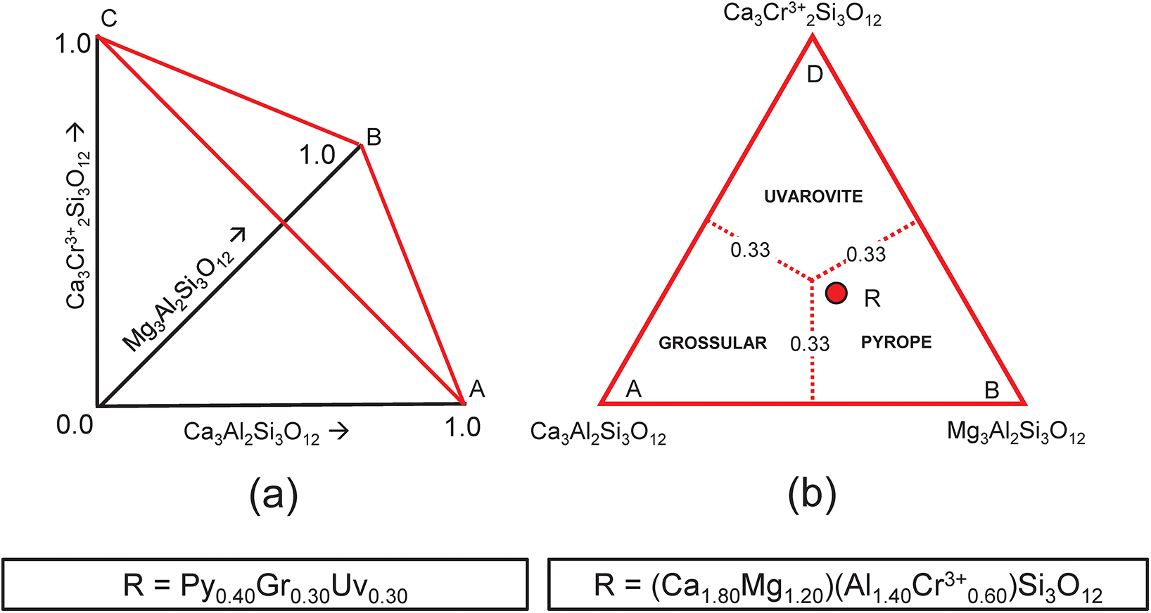
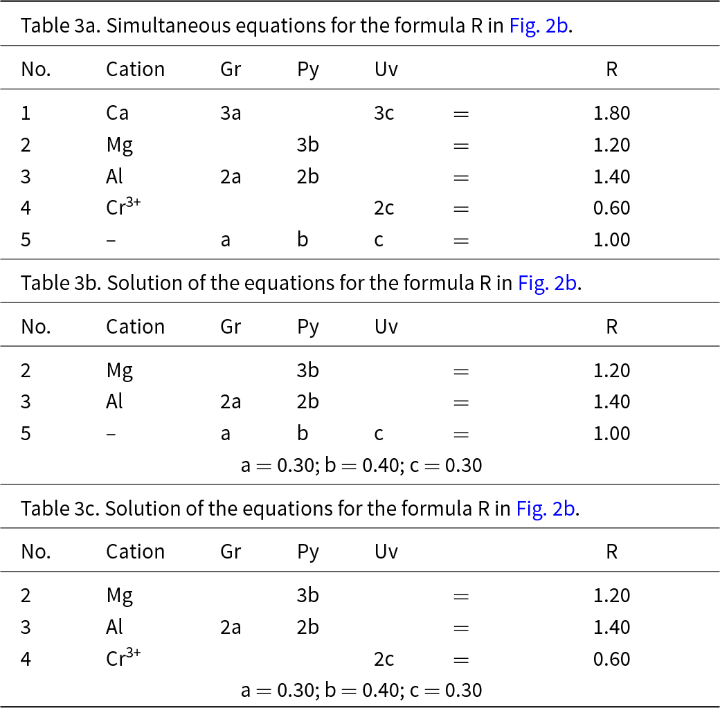
This system is slightly more complicated than the system grossular–andradite–uvarovite (Fig. 1) in which all ions in variable amounts occur at the Y-group and the X-group contains only Ca. In the system grossular–pyrope–uvarovite, variable amounts of ions occur at both the X-group (Ca and Mg) and the Y-group (Al and Cr³⁺) (Fig. 2a). Let R represent the garnet formula ^X(Ca_1.80Mg_1.20)^Y(Al_1.40Cr_0.60)^ZSi₃O₁₂, shown as the red circle in Fig. 2b. As above, we may write the simultaneous equations to express the formula in terms of its component end-members (Table 3a). There are five equations, but equations 1 and 2 are linearly related to equation 5, and equations 3 and 4 are linearly related to equation 5, and we may solve any linearly independent triplet of equations to get the amounts of component end-members as in Tables 3b and 3c.

Figure 2.

Compositional variation in the system Ca₃Al₂Si₃O₁₂–Mg₃Al₂Si₃O₁₂–Ca₃Cr³⁺₂Si₃O₁₂; (a) variation in each constituent from 0 to 1; the red triangle denotes the plane in which the three constituents sum to 1; note that the black axes labelled Ca₃Al₂Si₃O₁₂, Mg₃Al₂Si₃O₁₂ and Ca₃Cr³⁺₂Si₃O₁₂ in (a) are orthogonal; (b) the red triangle in (a) orientated in the plane of the page; the dotted red lines denote the boundaries between the compositional fields of grossular, pyrope and uvarovite; the red circle (labelled R) marks the formula (Ca_1.80Mg_1.20)(Al_1.40Cr³⁺_0.60)Si₃O₁₂.

Table 3.

Simultaneous equations for the formula R in Fig. 2

The system grossular–pyrope–knorringite–uvarovite

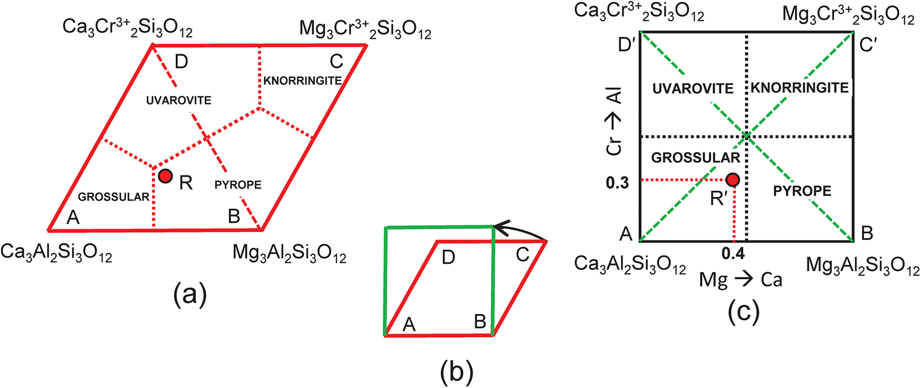
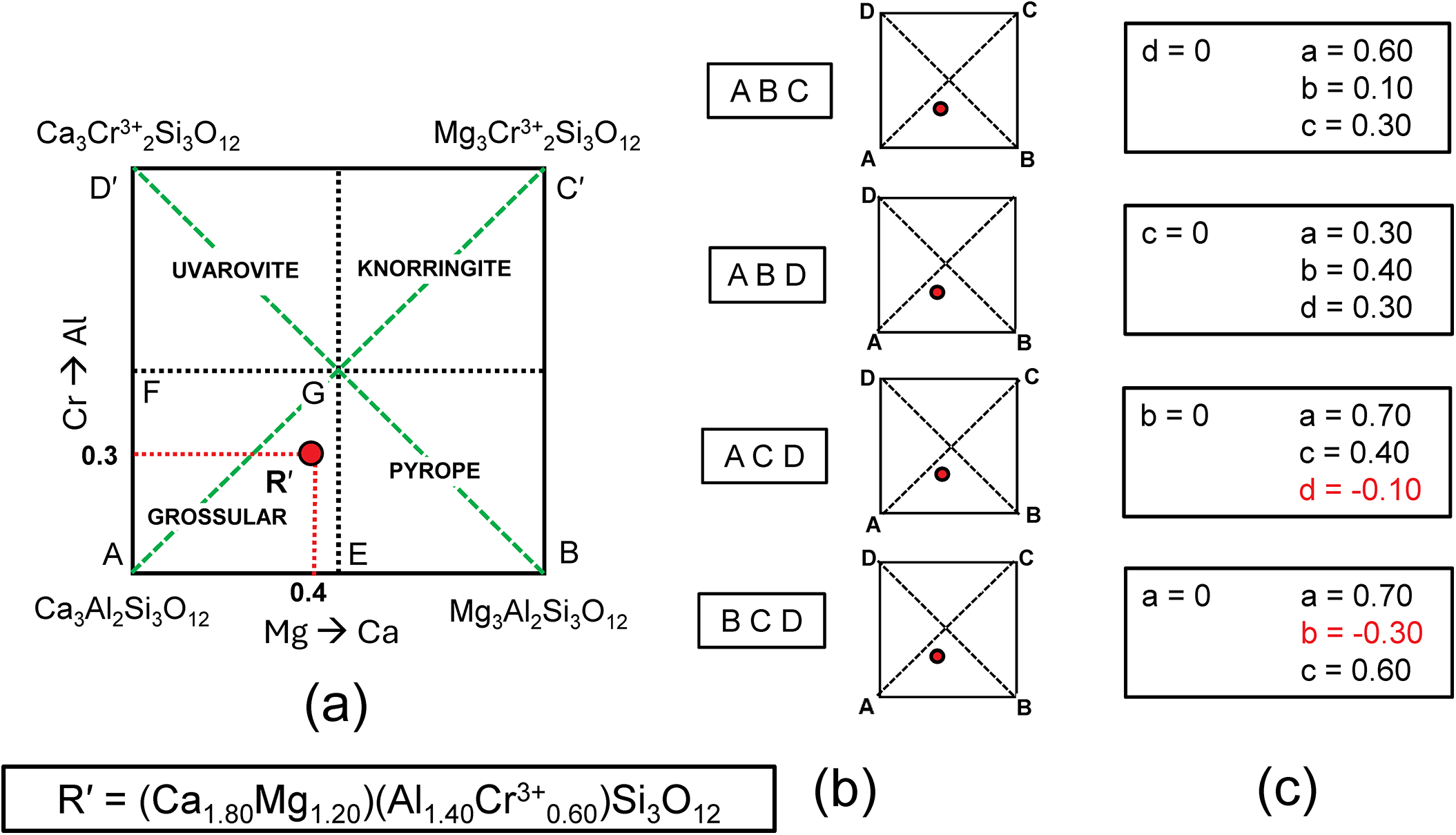
The end-member knorringite (Table 1), Mg₃Cr³⁺₂Si₃O₁₂, is also compatible with the garnet formula R = ^X(Ca_1.8Mg_1.2)^Y(Al_1.4Cr_0.60)Si₃O₁₂, so let us add it to the system: grossular–pyrope–knorringite–uvarovite. The end-member formula of knorringite is planar with Fig. 2b as shown in Fig. 3a, and the compositional ranges of each distinct mineral are shown with their boundaries as dotted red lines. We may produce a more convenient representation by rotating the edges AD and BC 30° anticlockwise (Fig. 3b) to produce a square diagram (Fig. 3c) of the type that is commonly used in Mineralogy. This rotation shifts point R from the compositional field of pyrope (Fig. 3a) to the compositional field of grossular (Fig. 3c) to point R′ as shown in Figs 3c and 4a, and as shown in Fig. 2b, point R′ (≡ R) corresponds to the composition (Ca_1.80Mg_1.20)(Al_1.40Cr³⁺_0.60)Si₃O₁₂. The diagonal dashed green lines in Fig. 3c correspond to the lines AC and BD in Fig. 3a.

Figure 3.

Compositional variation in the system Ca₃Al₂Si₃O₁₂–Mg₃Al₂Si₃O₁₂–Mg₃Cr³⁺₂Si₃O₁₂–Ca₃Cr³⁺₂Si₃O₁₂; (a) expressed as Fig. 2b with addition of an extra vertex C = Mg₃Cr³⁺₂Si₃O₁₂ and the compositional field of knorringite; the formula (Ca_1.80Mg_1.20)(Al_1.40Fe³⁺_0.60)Si₃O₁₂ is marked by the red circle R and occurs in the compositional field of pyrope; (b) vertices C and D of (a) are rotated 30° anticlockwise to produce a square outline to the diagram; (c) the internal contents of (a) are relocated accordingly; the red circle Rʹ now occurs within the compositional field of grossular.

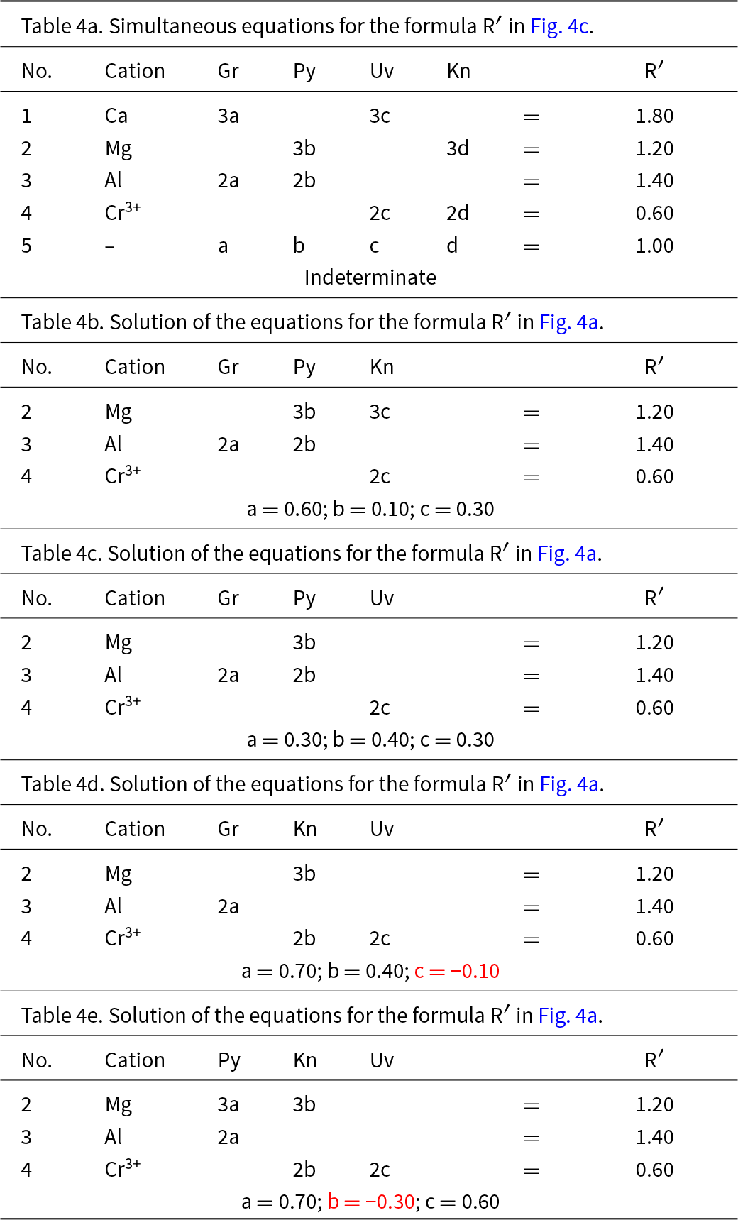
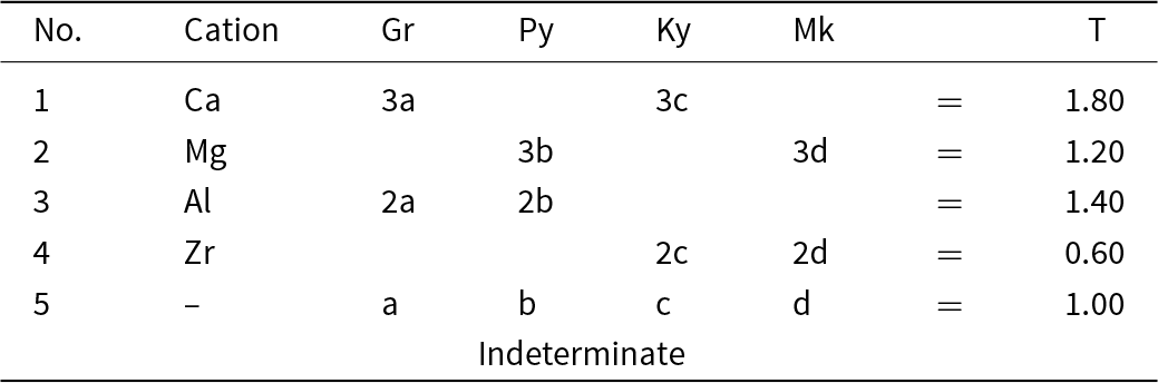
We may attempt to write the composition R′ in terms of the four end-members grossular, pyrope, knorringite and uvarovite, and the resulting set of equations is shown in Table 4a. As the substitution producing one of the end-members is linearly dependent on the other substitutions, the solution of these equations is indeterminate. This may be seen by assigning two arbitrary numbers to one variable and solving for the remaining variables. For example, let a = 0.4, from which b = 0.3, c = 0.2 and d = 0.10; let a = 0.5, from which b = 0.2, c = 0.1 and d = 0.20. Both these sets of numbers satisfy the equations of Table 4 and hence the system is indeterminate; unique solutions occur only where the end-members are linearly independent components.

Table 4.

Simultaneous equations for the formula R′ in Fig. 4

In Fig. 3c, there are diagonal (green dashed) lines, producing four triangles: in each of these triangles (ABC, ABD, ACD and BCD), the triplet end-members are linearly independent and should give solutions to the simultaneous equations describing the formula of R′. The relation of Fig. 4a and the formula R′ to the sets of component end-members is shown in Fig. 4b, and the solutions to the different sets of simultaneous equations are shown in Tables 4b–e and Fig. 4c. Of course, the solutions differ for different sets of end-members. Note also that where the formula R′ lies outside the triplet of components, one of the values of a, b, c and d is negative; the corresponding sets of values are algebraically correct although obviously not physically valid. So which of the solutions to the triplets ABC and ABD are correct for R′? They are both correct, and the issue comes down to which set of components one wishes to use. At this stage, which set to use is not apparent.

Figure 4.

(a) Compositional variation in the system Ca₃Al₂Si₃O₁₂–Mg₃Al₂Si₃O₁₂–Mg₃Cr³⁺₂Si₃O₁₂– Ca₃Cr³⁺₂Si₃O₁₂ as in Fig. 3c; (b) the four different triplets of component end-members ABCD and graphical representations of their relation to the complete system; (c) the resulting end-member proportions corresponding to the four triplets of component end-members found by solving the relevant simultaneous equations (with negative values shown in red).

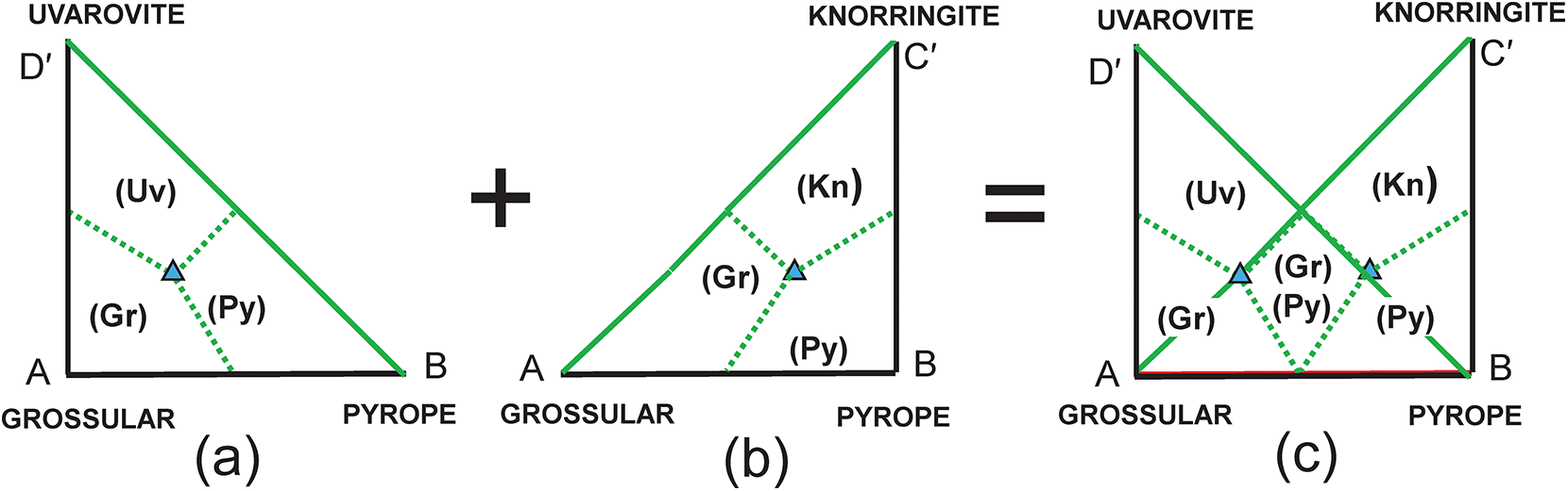
The composition R′ in Fig. 3c lies within two triplets of end-members: grossular–pyrope–uvarovite [Gr–Py–Uv] and grossular–pyrope–knorringite [Gr–Py–Kn]. Figures 5a,b show these two triangles extracted from Fig. 3c together with their compositional boundaries. If we superimpose these two triplets as in Fig. 5c, we produce the partial diagram in which there are five distinct compositional areas; there are four quadrilaterals in each of which a single end-member is dominant, and one quadrilateral in which one of two end-members is dominant depending on the triplet of component end-members used in the calculation. These results suggest that the name grossular cannot be assigned to compositions that lie within the square AEGF in Fig. 4a as use of the triplet of end-members grossular, pyrope and knorringite result in pyrope being the dominant end-member in some of these compositions.

Figure 5.

(a,b) The constituent triangles ABD′ and ABC′ from Fig. 3c; (c) the triangles ABD′ and ABC′ and their contents overlapped as in Fig. 3c. Note the central kite in which two dominant end-members are noted, marked by (Gr,Py).

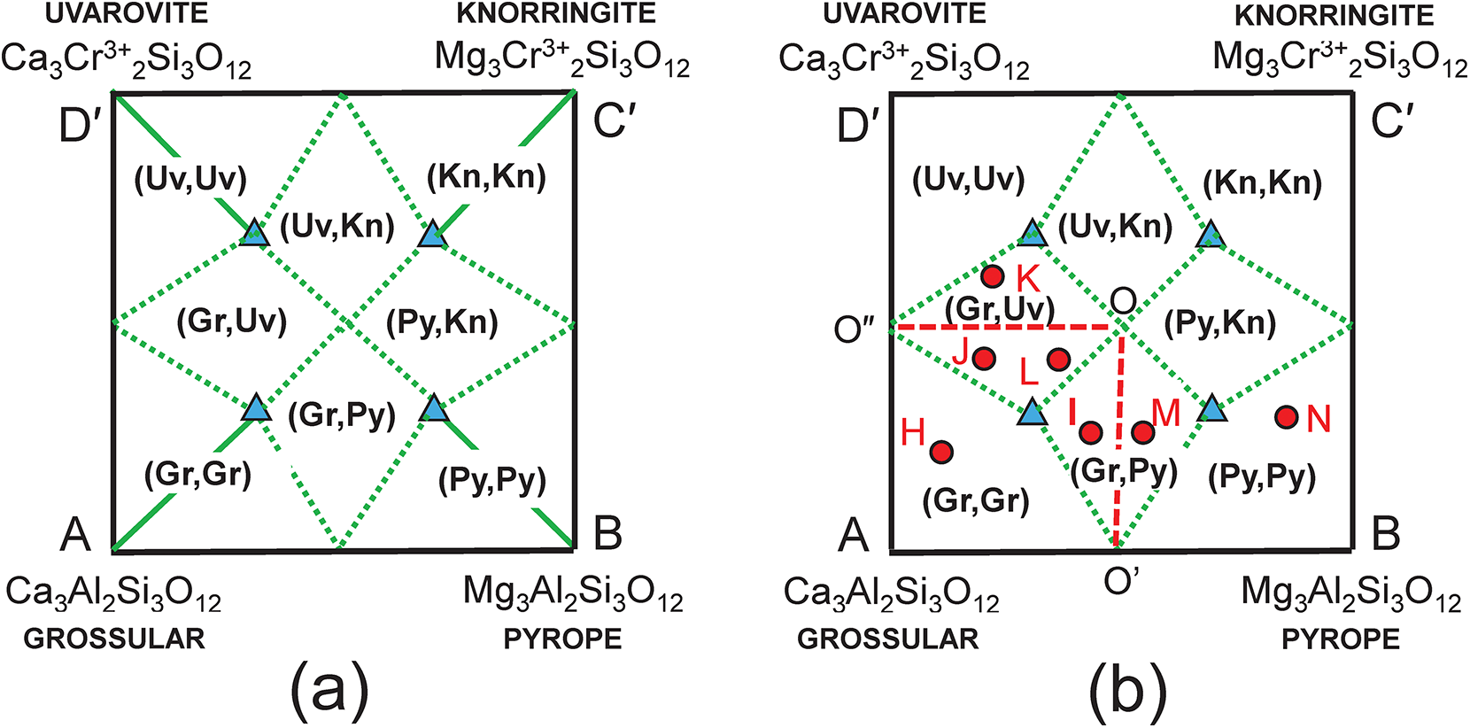
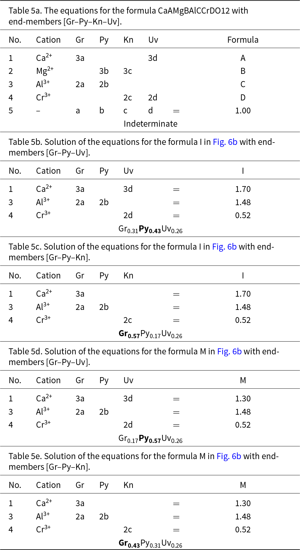
We may check the validity of the graphical construction in Fig. 5. Figure 6a shows the complete quadrilateral generated by the symmetry operations inherent in Figs 3c and 5c. There is a large central region of Fig. 6a in which there is ambiguity regarding the dominant end-member calculated with different triplets of component end-members. I examined this issue further by calculating the amounts of component end-members for numerous chemical compositions that fall within Fig. 6; a selection of these points is shown on Fig. 6b and examples of the calculations of their end-member proportions are shown in Table 5. Table 5a shows the relations between the formula of the garnet ^X(Ca_AMg_B)^Y(Al_CCr_D)Si₃O₁₂ and all the end-members: Gr, Py, Kn and Uv. As there is linear dependence between the four end-members, we must remove each one of them in turn and remove two other equations to get a solution. As was the case in Fig. 4, half of the solutions have negative amounts of component end-members and are omitted here. The physically valid solutions for compositions I and M in Fig. 6 are shown in Tables 5b–e. Let us examine the end-member proportions for points I (Tables 5b,c) and M (Tables 5d,e) for both triplets of component end-members, [Gr–Py–Uv] and [Gr–Py–Kn], respectively. For formula I, the dominant end-member is different for the two triplets, but collectively, Gr_0.57 (Table 5c) is dominant over Py_0.43 (Table 5b) and hence grossular is the collective dominant end-member. For point M, M = (Gr_0.17Py_0.57Uv_0.26) (Table 5d) and (Gr_0.43Py_0.31Kn_0.26) (Table 5e) and Py_0.57 is collectively dominant over Gr_0.43. Repeating these calculations for other formulae within the kite enclosing formulae I and M gives the same result. In Fig. 6b, all points to the left of the line OO′ have grossular (Gr) as the dominant end-member whereas all points to the right of the line OO′ have Py as the dominant end-member (when considering triplets of end-members that give solutions with only positive values of each end-member). The symmetry of Fig. 6b indicates that this pattern of end-member dominance will be maintained in the various central sectors of the figure. Points J, K and L show a similar pattern of end-member dominance: J = (Gr_0.37Py_0.21Uv_0.42) and (Gr_0.58Kn_0.21Kn_0.21), and Gr is dominant over Uv; K = (Gr₀₁₈Py_0.22Uv_0.60) and (Gr_0.40Kn_0.22Uv_0.38), and Uv is dominant over Gr; L = (Gr_0.37Py_0.21Uv_0.42) and (Gr_0.58Kn_0.37Kn_0.05), and Gr is dominant over Uv. Calculations for many other chemical formulae confirm this pattern of end-member dominance.

Figure 6.

Compositional variation in the system Ca₃Al₂Si₃O₁₂–Mg₃Al₂Si₃O₁₂–Mg₃Cr³⁺₂Si₃O₁₂– Ca₃Cr³⁺₂Si₃O₁₂; (a) completion of the process illustrated in Fig. 5 in all constituent triangles of Fig. 3c; (b) example compositions from H to N for which the dominant end-members were calculated and expressed by paired letters, e.g. (Gr,Gr) or (Gr,Py).

Table 5.

The equations for the formula Ca_AMg_BAl_CCr_DO₁₂ with end-members [Gr–Py–Kn–Uv]

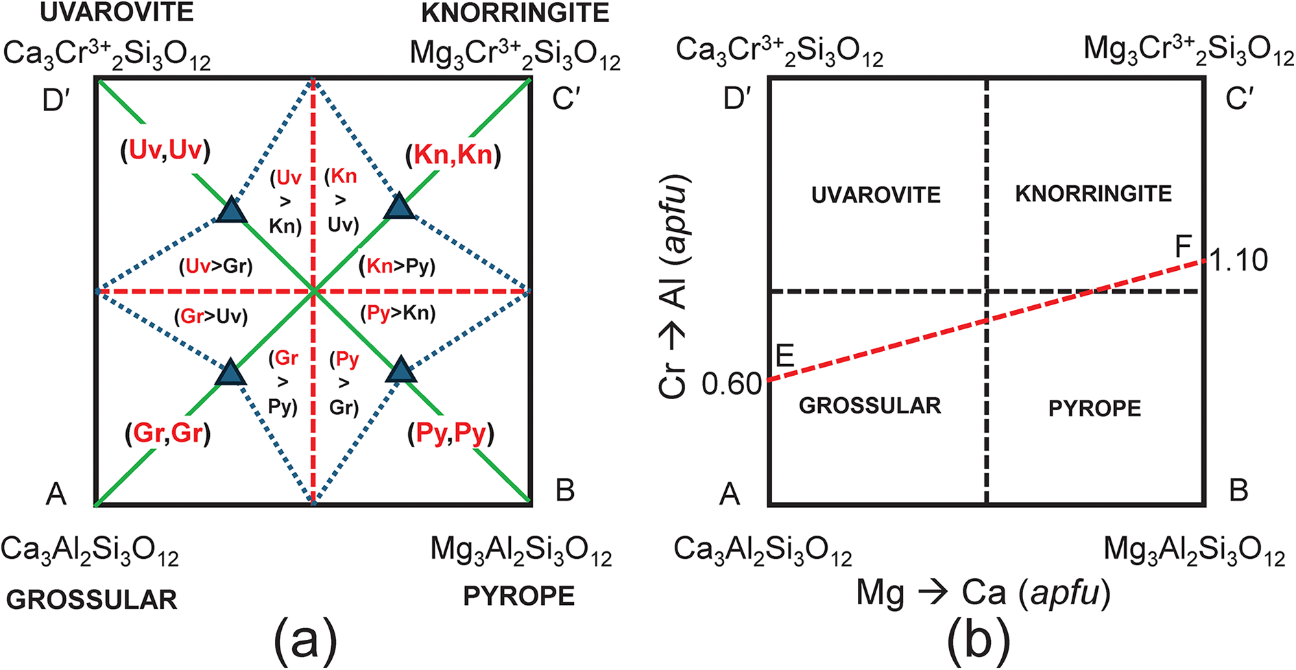
This behaviour is generalised in Fig. 7a which shows that for any chemical formula with ^XCa ≥ 1.50 apfu and ^YAl ≥ 1.00 apfu, grossular is the dominant end-member, and similar constraints define the compositional ranges for which pyrope, knorringite and uvarovite are the dominant end-members (Fig. 7b). This is an important result not just for garnets, as compositional variation in many minerals is shown graphically on diagrams resembling Fig. 7b, and mineral names are assigned to specific mineral compositions using rectangular diagrams in which linearly dependent end-member compositions are used as vertices of the diagrams.

Figure 7.

(a) Complete representation of the system Ca₃Al₂Si₃O₁₂–Mg₃Al₂Si₃O₁₂–Mg₃Cr³⁺₂Si₃O₁₂–Ca₃Cr³⁺₂Si₃O₁₂ showing the dominant end-member in every internal triangle of the diagram; (b) the system Ca₃Al₂Si₃O₁₂–Mg₃Al₂Si₃O₁₂–Mg₃Cr³⁺₂Si₃O₁₂–Ca₃Cr³⁺₂Si₃O₁₂ showing the dominant end-member in each quadrant; also shown is the join EF along which the end-member proportions are calculated.

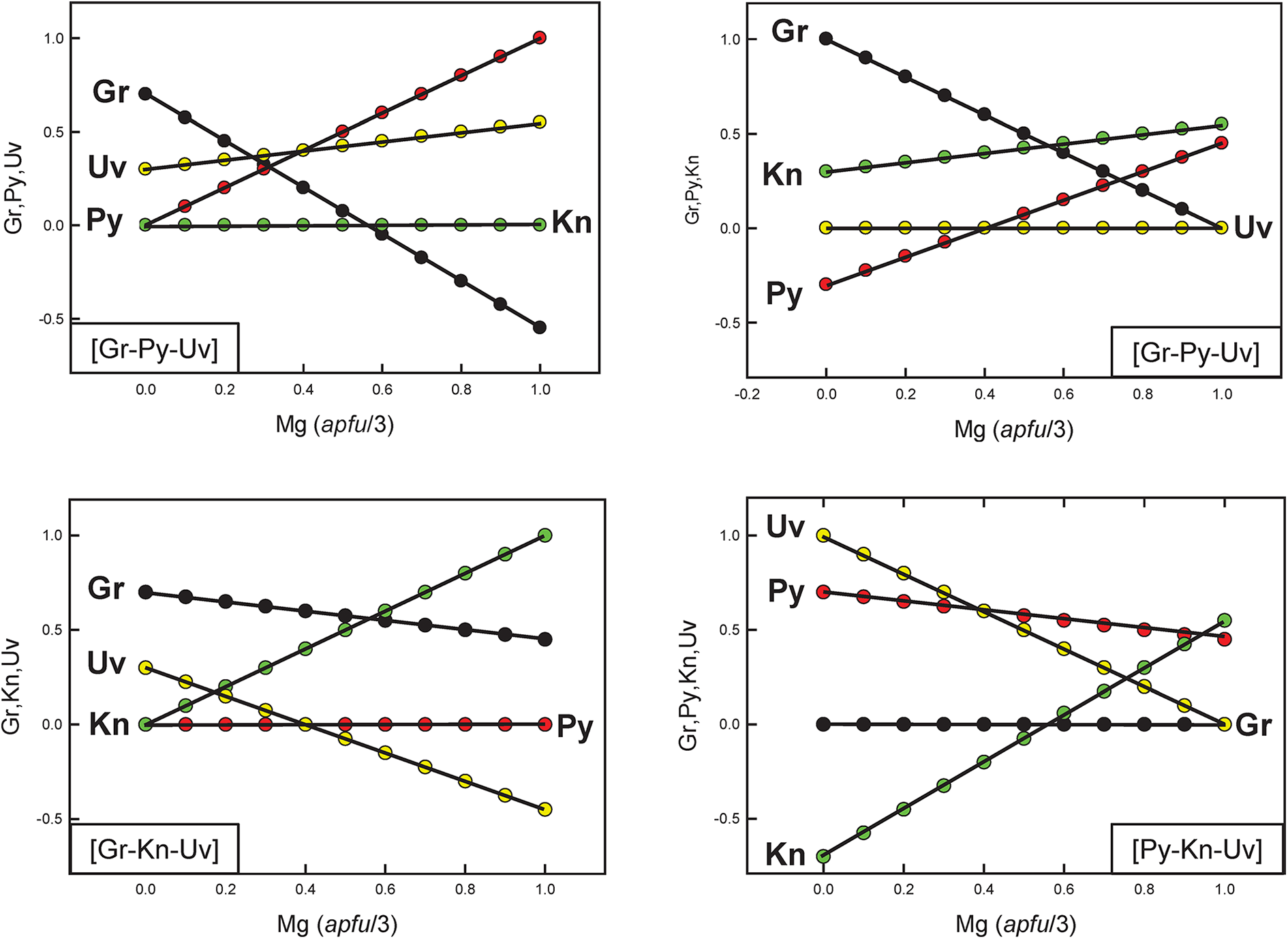
It is important to realise that although chemical formulae are correctly represented in Fig. 7b, the corresponding end-member proportions are not, except for the identity of the dominant end-member. For example, consider compositions lying along the line EF in Fig. 7b. The variation in end-member proportions as a function of chemical composition for each triplet of independent end-members is shown in Fig. 8. Along the join EF, for each triplet, the proportions of each end-member have the following features: (1) the end-member that is missing from the triplet of components is, of course, zero along the entire length of the join; (2) one end-member is negative along part of the join; (3) one end-member varies from 0 to 1. However, it is apparent that there are no useful regularities of end-member composition along the joint EF, or by implication, within the quadruplet [Gr–Py–Kn–Uv], apart from identification of the dominant end-member as indicated in Fig. 7b.

Figure 8.

The variation in end-member proportions along the join EF in Fig. 7, calculated using the end-member triplets indicated in the bottom left or bottom right of each diagram.

All origin formulae in the pyralspite–ugrandite system

Deer et al. (Reference Deer, Howie and Zussman1992) and Hawthorne (Reference Hawthorne2021b) showed that one specific garnet formula containing all possible cations in the pyralspite–ugrandite system, (Mg_1.82Fe²⁺_0.79Mn_0.02Ca_0.37) (Al_1.92Fe³⁺_0.06Cr_0.02)Si₃O₁₂, can be assigned end-member proportions involving the six end-members PyAlSpUvGrAn. On the other hand, the composition Ca₃Al₂Si₃O₁₂ is uniquely described by one end-member formula. This raises the question of how many subsystems there are within the system of twelve end-members listed in Table 1 that may describe all possible garnet formulae within the pyralspite–ugrandite system involving only linearly independent end-members. Inspection of Table 1 shows that there are four X cations and three Y cations associated with all possible chemical formulae within this system, in accord with the number of possible cation arrangements in the pyralspite–ugrandite garnets: ^X4 × ^Y3 = 12. The maximum possible number of cations in a specific garnet composition of this type is ^X4 + ^Y3 = 7 and the sum of these cations is fixed at 5 apfu (the sum of the X- and Y-groups). Hence there is a maximum of six unknowns required in the pyralspite–ugrandite system to describe all possible compositions. Such compositions may be quantitatively expressed in terms of six (or less) end-members, providing that these end-members are linearly independent, as is the case for grossular, andradite, uvarovite, pyrope, almandine and spessartine (Table 1). By sequentially selecting each end-member composition in Table 1 as the origin formula, all linearly independent tupletFootnote ¹ subsystems within these twelve end-members may be derived if needed.

Calculation of the dominant end-member formulae in pyralspite–ugrandite garnets

Although the above discussion of calculation of end-member proportions may seem complicated, the identification of the dominant end-member formulae in pyralspite–ugrandite garnets is no more complicated than the calculation of a mineral formula. Using a spreadsheet program (e.g. Excel^©) or mathematics software (e.g. MATLAB^©), large numbers of analyses can be processed to derive the dominant end-member name and formula.

Addition of heterovalent compositional variations

The above systems involve only homovalent substitutions and hence apply only to one constituent-cation charge arrangement (Hawthorne, Reference Hawthorne2002, Reference Hawthorne2021a). The situation becomes more complicated where heterovalent substitutions are involved because electroneutrality must be maintained.

The system grossular–pyrope–kimzeyite

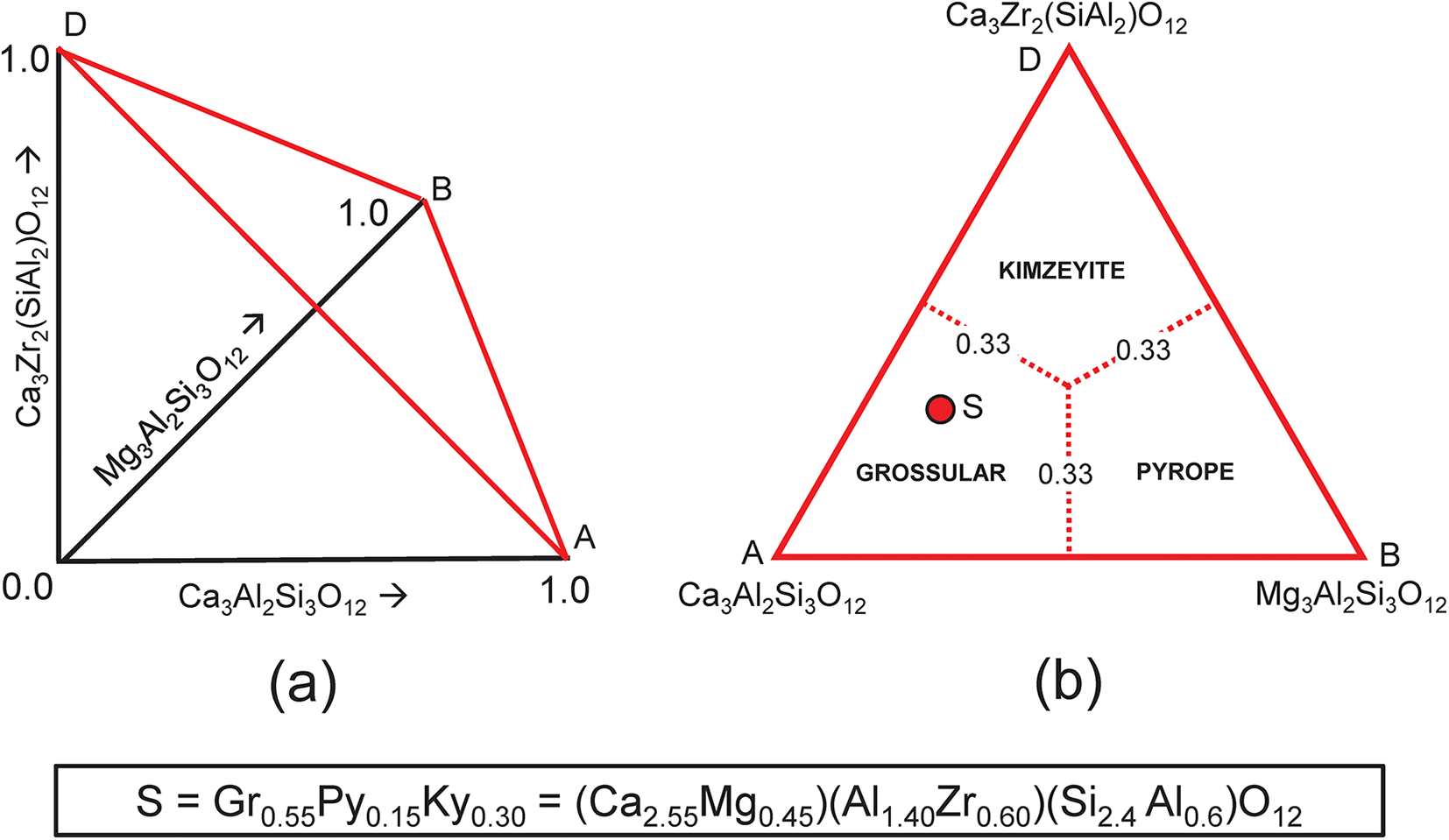
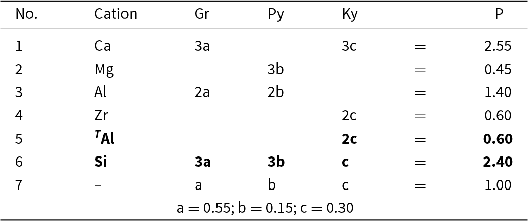
Consider the system grossular–pyrope–kimzeyite (Ca₃Zr₂(SiAl₂)O₁₂) (Fig. 9a,b) in which is plotted the composition S = (Ca_2.55Mg_0.45)(Al_1.40Zr_0.60)(Si_2.4 Al_0.6)O₁₂. We may write the set of simultaneous equations describing its chemical formula in terms of end-members as shown in Table 6. We have added an additional two compositional variables: ^ZAl and Si, which gives us five equations and only three unknowns. However, these two additional equations for ^ZAl and Si (Table 6, bold) are linear combinations of other equations in the set: that for ^ZAl is identical to that for Zr, and that for Si is identical to those for Ca, Mg and Al: Si = 3a + 3b + c = Ca + Mg – Zr. Thus, we may delete these two equations from the set and we get the unique solution shown in Table 6.

Figure 9.

(a,b) Compositional variation in the system Ca₃Al₂Si₃O₁₂–Mg₃Al₂Si₃O₁₂–Ca₃Zr₂(SiAl₂)O₁₂; (a) variation in each constituent from 0 to 1; the red triangle denotes the plane in which the three constituents sum to 1; note that the black axes labelled Ca₃Al₂Si₃O₁₂, Mg₃Al₂Si₃O₁₂ and Ca₃Zr₂(SiAl₂)O₁₂ in (a) are orthogonal; (b) the red triangle in (a) orientated in the plane of the page; the dotted red lines denote the boundaries between the compositional fields of grossular, andradite and uvarovite; the red circle S marks the formula (Ca_2.55Mg_0.45)(Al_1.40Zr_0.60)(Si_2.40Al_0.60)O₁₂.

Table 6.

Simultaneous equations for the formula P in Fig. 9

The system grossular–pyrope–Mg₃Zr₂(SiAl₂)O₁₂–kimzeyite

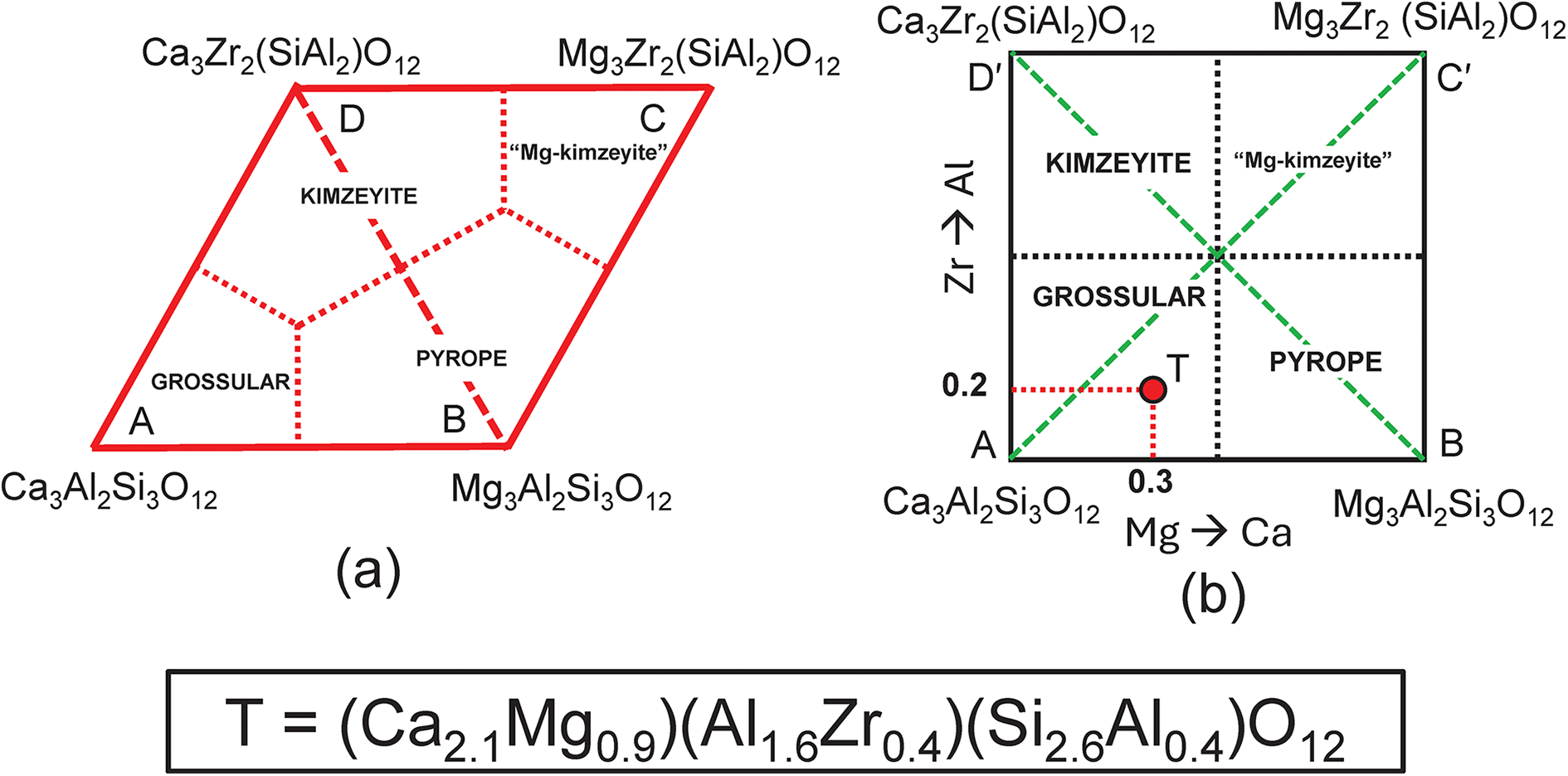
Next, we need to add a new end-member to the system grossular–pyrope–kimzeyite with a formula that is a linear combination of these end-members. There is no suitable garnet mineral but the formula Mg₃Zr₂(SiAl₂)O₁₂ will suffice (this is the Mg-analogue of kimzeyite). This system is shown in Fig. 10a,b on which is plotted the composition T = (Ca_2.1Mg_0.9)(Al_1.6Zr_0.4)(Si_2.6Al_0.4)O₁₂. The corresponding matrix of simultaneous equations is given in Table 7; the system is indeterminate. We may remove equations that are linearly related to other equations and solve for the end-member proportions for each distinct set of component end-members as was done for the system grossular–pyrope–knorringite–uvarovite (see above, Table 4 and Fig. 4). The dominant end-member formula for garnet T is grossular, in accord with the fact that formula T lies within the compositional field of grossular in Fig. 10b.

Figure 10.

Compositional variation in the system Ca₃Al₂Si₃O₁₂–Mg₃Al₂Si₃O₁₂–Mg₃Zr₂(SiAl₂)O₁₂– Ca₃Zr₂(SiAl₂)O₁₂; (a) expressed as Fig. 9b with addition of an extra vertex C = Mg₃Zr₂(SiAl₂)O₁₂ and the compositional field of ‘Mg-kimzeyite’; (b) expressed in orthogonal axes; the formula (Ca_2.10Mg_0.90)(Al_1.60Zr_0.40)(Si_2.60Al_0.40)O₁₂ is marked by the red circle T and occurs in the compositional field of grossular.

Table 7.

Simultaneous equations for the formula T in Fig. 10b

Calculation of the dominant end-member formula for a complex garnet

The above examples were developed by defining a set of end-member formulae, selecting a formula that lay within this system, and examining the issues associated with defining the dominant end-member formula. When dealing with the empirical chemical formula of a mineral grain, one is faced with the inverse problem of defining a set of end-member formulae that contain the formula of the mineral of interest rather than defining a mineral formula that fits a predetermined set of component end-members.

Calculation of end-member constituent-cation charges

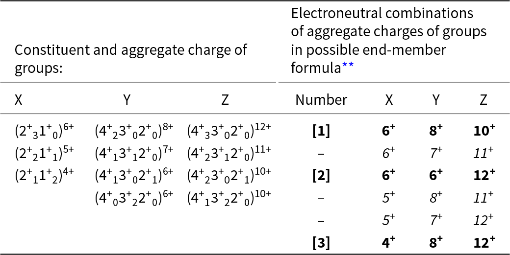
An end-member constituent-cation charge arrangement is a distinct arrangement of aggregate charges of the cation groups. In garnet, this involves arrangements of constituent-cation charges over the X-, Y- and Z-groups of cations. Inspection of the chemical formula of the Ice River garnet shows that the ranges of charge of the cations in each group are as follows: X: 2⁺, 1⁺; Y: 4⁺, 3⁺, 2⁺; Z: 4⁺, 3⁺, 2⁺. However, not all combinations of these charges are possible because of the constraint of electroneutrality. For example, the possible combinations of cations in the X-group are (2⁺₃1⁺₀), (2⁺₂1⁺₁), (2⁺₁1⁺₂), (2⁺₀1⁺₃) for aggregate charges of 6⁺, 5⁺, 4⁺, 3⁺; all the arithmetically possible combinations for the Y- and Z-groups give the possible aggregate charges: Y: 8⁺, 7⁺, 6⁺, 5⁺, 4⁺; Z: 12⁺, 11⁺, 10⁺, 9⁺, 8⁺, 7⁺, 6⁺. Consider the X-group aggregate charge of 3⁺: the maximum aggregate charges of the Y- and Z-group cations are 8⁺ and 12⁺, and the electroneutrality requirement of 24⁺ cannot be satisfied by an X-group aggregate charge of 3⁺ and thus an X-group aggregate charge of 3⁺ cannot occur. The electroneutrality constraint restricts the aggregate charges of the X-, Y- and Z-group cations to the values given in Table 8. The sets of aggregate charges at the X-, Y- and Z-groups of cations must contain either none or one aggregate charge of two differently charged ions if they are to constitute a set of aggregate-charge arrangements for an end-member; the charge arrangements that do not accord with this requirement are shown in italics in Table 8. There are three distinct end-member sets of aggregate-charge arrangements and these are labelled [1], [2] and [3] in Tables 8 and 9.

Table 8.

Possible constituent and aggregate charges in each cation group*, and possible combinations of electroneutral arrangements of aggregate charges of the cation groups for possible end-members for a garnet from Ice River. ^X[Ca_2.86Mg_0.10Na_0.04]_Σ3^Y[Ti_1.06Fe³⁺_0.65Al_0.14Fe²⁺_0.04Zr_0.04Mg_0.04Mn_0.03]_Σ2^Z[Si_2.35Fe³⁺_0.35Fe²⁺_0.30]_Σ3

* Aggregate charges for each cation group are shown as superscripts to the combinations of constituent-cation charges in each group;

** Those combinations in italics cannot represent end-members as they involve more than one charge species at more than one site.

Calculation of constituent-cation charge of each cation group

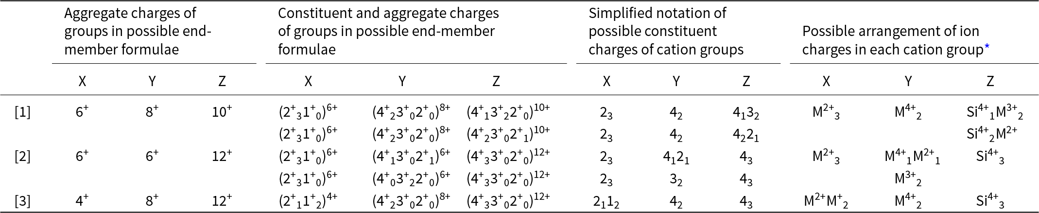
For each distinct aggregate-charge arrangement for end-members (Table 9, column 1), we may calculate the combinations of possible integral charges from the set of cations in each cation group (X, Y or Z) for the Ice River garnet. This is done in the second set of columns in Table 9 and a simplified version is given in the third set of columns in the same table. The last set of columns interprets these charges in terms of cations of different charge in the Ice River garnet: M⁺ = Na⁺; M²⁺ = Ca²⁺, Mg²⁺, Fe²⁺ and Mn²⁺; M³⁺ = Al³⁺, Fe³⁺; M⁴⁺ = Ti⁴⁺, Zr⁴⁺; plus Si⁴⁺.

Table 9.

Possible arrangements of constituent-cation charges in each cation group of Ice River garnet

* ^XM²⁺ = Ca²⁺ and Mg^{2+; X}M⁺ = Na^{+; Y}M²⁺ = Fe²⁺, Mg²⁺ and Mn^{2+; Y}M³⁺ = Fe³⁺ and Al^{3+; Y}M⁴⁺ = Ti⁴⁺ and Zr^{4+; Z}M²⁺ = Fe^{2+; Z}M³⁺ = Fe³⁺ and Al³⁺.

Calculation of all relevant end-member formulae

We may derive the component end-member formulae by incorporating the relevant ions from the chemical formula of Ice River garnet (see above) into the garnet structure such that they are conformable with the possible end-member constituent-cation charge arrangements (Table 8). This procedure results in 28 distinct end-member formulae, a considerable number. The complexity (sensu lato) of the formula of Ice River garnet raises a significant issue that has been mentioned in point [4] above. When we consider the chemical formula of a mineral, we generally restrict ourselves to the major and perhaps some minor elements and ignore trace elements. Obviously, this approach is not completely rigorous, but the intent of the present work is to derive the dominant end-member formula for a specific garnet chemical formula and a minor ion will generally not be of sufficient amount to form the dominant component end-member. For example, the X group contains 0.10 Mg apfu with a site occupancy of 0.10/3 = 0.033 ions per site. Half of the 28 end-member formulae contain Mg₃; thus even if all Mg were concentrated into one end-member, the fraction of that end-member in the Ice River garnet would only be 0.033, which obviously cannot be the dominant component end-member. Thus we ignore ^XMg in the formula of Table 8, including it with ^XCa; of course, this will increase the fraction of end-members containing ^XCa by 0.033, but as this amount is partitioned over up to 12 end-member formulae, it is extremely unlikely to materially affect the relative amounts of the end-member formulae containing ^XCa. Consequently, we may discard the 12 end-member formulae containing ^XMg, and the remaining end-member formulae are listed in Table 10 where they are each identified by a number.

Table 10.

End-member constituents for Ice River garnet

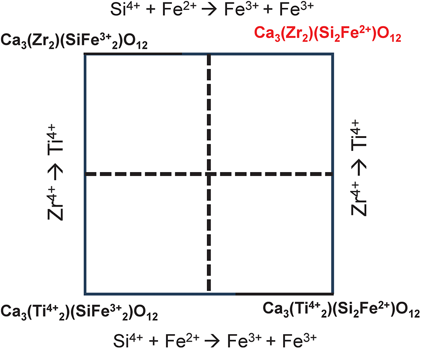
We may write a set of simultaneous equations relating the amounts of the end-members to the chemical formula of the Ice River garnet with the amounts of the end-members as unknowns in the set of equations. However, before solving this set of equations, we need to identify those end-member formulae of Table 10 that are not linearly independent of the other end-member formulae. For example, Fig. 11 shows that end-member 4, Ca₃Zr₂(Si₂Fe²⁺)O₁₂ (Table 10), is linearly dependent on end-members 1, 2 and 3. Thus end-member 4 must be omitted from the set of simultaneous equations relating the amounts of the end-members to the chemical formula of Ice River garnet. Identification of the other linearly dependent end-members is left as an exercise for the reader. The system of equations is still overdetermined and hence one additional end-member is removed from the set of equations; which end-member is removed is more-or-less arbitrary as the stoichiometry of the garnet determines the amount of this omitted end-member (cf. Tables 2 and 3).

Figure 11.

The compositional diagram Ca₃(Ti⁴⁺₂)(SiFe³⁺₂)O₁₂–Ca₃(Ti⁴⁺₂)(Si₂Fe²⁺)O₁₂–Ca₃(Zr₂)(Si₂Fe²⁺)O₁₂–Ca₃(Zr₂)(SiFe³⁺₂)O₁₂. The end-members are linearly dependent; Ca₃(Zr₂)(Si₂Fe²⁺)O₁₂ (in red) was omitted from the initial calculation of the end-member proportions (Tables 10 and 11).

Calculation of the amounts of the component end-members

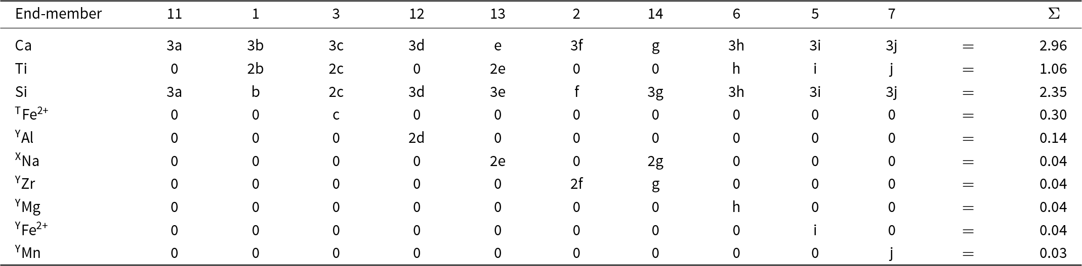
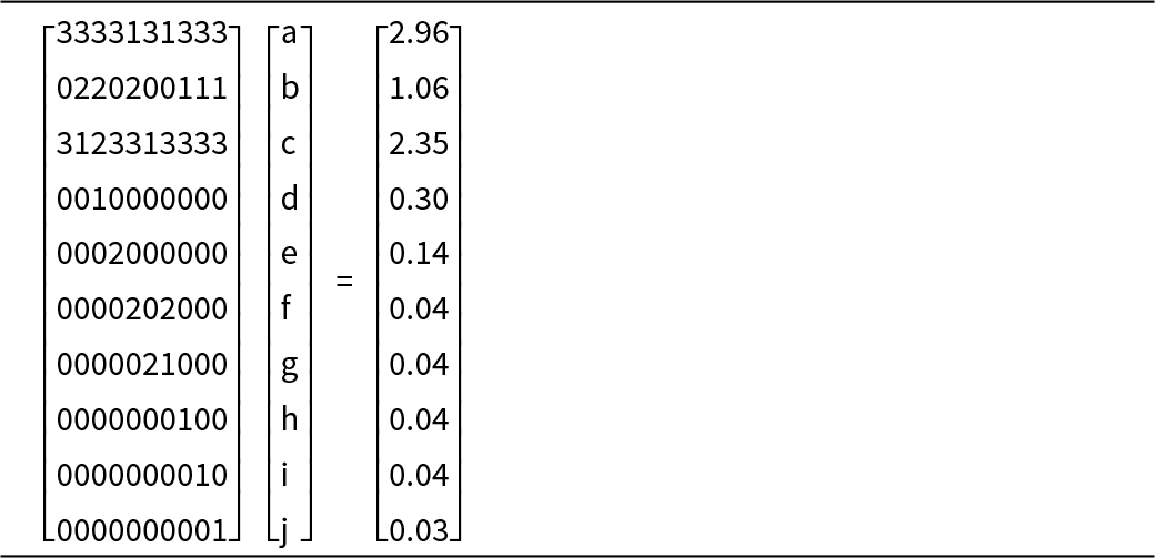
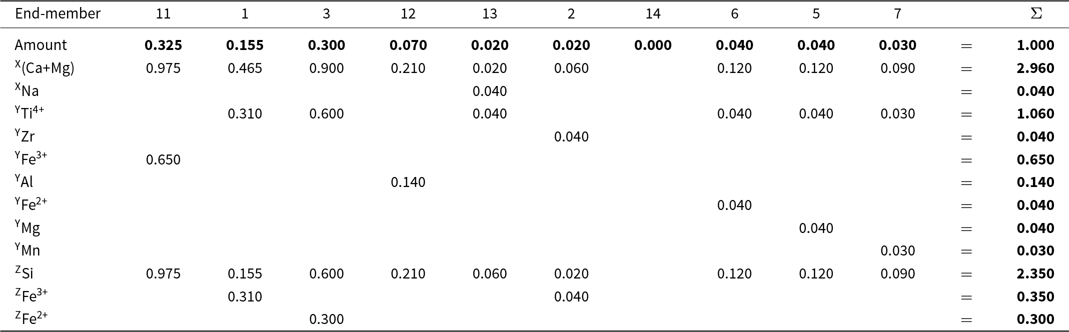
The final set of equations is given in Table 11. The equations in Table 11 are too complicated to be solved easily by hand. Table 12 expresses them in matrix form; they may be solved by Gaussian elimination using MATLAB^©. The solution is given in bold font in row 2 of Table 13. Table 13 also shows calculation of the chemical formula of the Ice River garnet from the calculated amounts of the component end-members; the solution is given in bold font in the last column on the right and it agrees with the experimental chemical formula listed at the bottom of the table.

Table 11.

Simultaneous equations relating the amount of each end-member to the chemical formula of Ice River garnet

Table 12.

Matrix equation for the amounts of component end-members in Ice River garnet

Table 13.

Calculation of Ice River garnet formula* from amounts of end-members

* Ice River garnet formula (see text): ^X[Ca_2.86Mg_0.10Na_0.04] ^Y[Ti_1.06Fe³⁺_0.65Al_0.14Fe²⁺_0.04Zr_0.04Mg_0.04Mn_0.03] ^Z[Si_2.35Fe³⁺_0.35Fe²⁺_0.30] O₁₂.

Other solutions

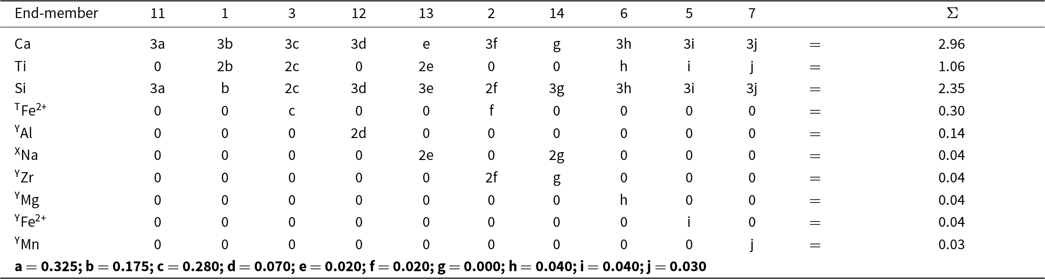
Where there are linearly dependent end-members in the original system of equations, it is arbitrary which dependent end-members are excluded as their inclusion will cause the composition matrix to be indeterminate (see for example Fig. 4). Thus we must repeat the calculation for Ice River garnet with all of the possible linearly dependent end-members excluded. Figure 11 shows that end-members 1, 2, 3 and 4 are not linearly independent and we excluded end-member 4, Ca₃Zr₂(Si₂Fe²⁺)O₁₂ (shown in red in Fig. 11), for the calculation of Table 11. However, the choice of which of the end-members 1, 2, 3 and 4 to exclude was arbitrary as any one of the formulae can be expressed in terms of the remaining three formulae. Thus we need to repeat the calculation for all possible triplets of 1, 2, 3, 4. When we do this, two of the four solutions give negative values for the amounts of some end-members; these solutions are algebraically correct but physically not possible (as shown for a garnet composition in Fig. 4) and the workings for these solutions are omitted. Table 14 shows the matrix of simultaneous equations for the other triplet that gives a physically realistic solution (shown in the last row of Table 14). Although the solutions to the sets of equations in Tables 11 and 14 are different (as is the case for the physically realistic solutions of a simpler garnet composition shown in Fig. 4), the dominant end-member is the same in each case: end-member 11. As the ^YZr content of the Ice River garnet is 0.04 apfu, the maximum difference in the amounts of the end-members is 0.020 (for end-members 2 and 3, cf. Tables 13 and 14).

Table 14.

Alternative set of simultaneous equations relating the amount of each end-member to the chemical formula of Ice River garnet

The end-members 5 to 10 (Table 10) also have linearly dependent relations between them and the calculations can be repeated for all of these possibilities. However, the calculation of Tables 11 and 14 indicate that we do not need to do this. The maximum amounts of the constituents ^YZr (0.04 apfu), ^YMg (0.04 apfu), ^YFe²⁺ (0.04 apfu) and ^YMn (0.03 apfu) indicate that the physically possible solutions cannot differ by more than 0.020 [the amount of the constituent in the empirical formula divided by the rank of the B-group (2) to which they belong]. Changes of this magnitude cannot alter the dominant end-member and hence we conclude that the Ice River garnet is 11: andradite (not schorlomite).

Without recalculating all chemical analyses of garnet identified as schorlomite (end-member formula Ca₃Ti⁴⁺₂(SiFe³⁺₂)O₁₂, Grew et al., Reference Grew, Locock, Mills, Galuskina, Galuskin and Hålenius2013), I cannot comment on the status of schorlomite as a valid species. However, the situation with regard to Ti⁴⁺-rich garnets has become more complicated as calculation of the end-member components for the Ice River garnet also suggests that Ca₃Ti⁴⁺₂(Si₂Fe²⁺)O₁₂ is a potential dominant end-member for Ti-rich garnets in addition to schorlomite (Ca₃Ti⁴⁺₂(SiFe³⁺₂)O₁₂).

The significance of the above results to defining and determining mineral species

Hawthorne (Reference Hawthorne2023a, Reference Hawthorne2023b) considered the rules of the IMA–CNMNC for defining distinct mineral species and showed that there are significant problems with the approach based on the rule of the dominant constituent (Hatert and Burke, Reference Hatert and Burke2008) and its ensuing modifications. The alternative approach is the dominant-end-member method (Bulakh, Reference Bulakh2010; Dolivo-Dobrovol’sky, Reference Dolivo-Dobrovol’sky2010) in which all minerals of a species have the end-member formula of that mineral as their dominant end-member. However, as noted by Hawthorne (Reference Hawthorne2023a), there are currently unresolved issues associated with this dominant-end-member approach. These ‘unresolved issues’ involve (1) the use of end-member formulae as phase components, and (2) the use of mineral formulae that violate the laws of Physics.

Coda

(1) For end-member formulae to be phase components of a mineral formula, the end-member formulae must be linearly independent.

(2) In order to do end-member calculations, (i) the associated mineral formula must be electroneutral; (ii) the crystallographic sites must be completely occupied by ions and vacancies that are stoichiometrically part of the formula of the mineral; and (iii) there can be no cations in excess of what can be accommodated by the crystallographic sites of the structure.

(3) If the end-member formulae used are phase components of the mineral, the proportions of end-members may be calculated exactly by solving the set of simultaneous equations that relate the amount of each end-member to the formula of the mineral.

(4) If one attempts to use (as phase components) one or more end-members that are linear combinations of other end-members, the system of equations is indeterminate.

(5) In a system that contains an end-member that is a linear combination of other end-members, one may remove that end-member from the system to produce a set of equations that may be solved exactly. However, there will be several sets of end-members that may be used as phase components, and each set will give a different solution for the end-member proportions of the mineral. If the mineral formula lies within the bounds of the end-members, the calculated end-member proportions are all positive; if the mineral formula lies outside the bounds of the end-members, one or more of the calculated end-member proportions are negative.

(6) For those solutions involving end-member proportions in which every term is positive, the dominant end-member may differ for the different sets of component end-members. However, inspection of composition space shows that the solution with the highest value of its dominant end-member is consistent with the name of the mineral indicated by its chemical composition. Only the dominant end-member is so indicated; the end-member proportions obtained are not valid.

(7) Thus the chemical composition of the mineral indicates its dominant component end-member, and hence the mineral can be defined as a particular species by its dominant component end-member.