


Introduction
High-resolution records of the isotopic composition of polar ice cores provide a detailed picture of past climate spanning hundreds of thousands of years (Johnsen and others, Reference Johnsen2001; EPICA Community Members, Reference EPICA Community Members2004, Reference EPICA Community Members2006; NEEM Community Members, Reference NEEM Community Members2013; WAIS Divide Project Members, Reference WAIS Divide Project Members2015). These records carry palaeoclimatic information that can be used in order to estimate past temperatures and accumulation rates. Analytical techniques based on high throughput mass spectrometry systems, as well as laser Cavity Ring Down Spectrometry coupled to continuous melting devices (Gkinis and others, Reference Gkinis2011; Emanuelsson and others, Reference Emanuelsson, Baisden, Bertler, Keller and Gkinis2015; Jones and others, Reference Jones2017b), have yielded isotopic records of very high resolution in the order of centimetres or below. In addition to their obvious potential to resolve climate signals at shorter time scales, these records open new possibilities for studies targeting the information stored in the spectral domain of the isotopic time series (Gkinis and others, Reference Gkinis, Simonsen, Buchardt, White and Vinther2014; Jones and others, Reference Jones2018).
A well-documented example, where knowledge of the spectral signature of the isotopic time series is useful, is the characterisation of the post-depositional diffusive process that attenuates the initial isotopic signal of the precipitation, affecting particularly its high frequency bands. This diffusive process can also alter the signal to noise ratio on certain frequency bands of the δ18O signal, thereby inducing a seemingly multi-decadal variability commonly measured at low accumulation Antarctic sites (Laepple and others, Reference Laepple2018). Isotopic diffusion takes place first in the gas phase, within the porous medium of polar firn as it densifies and later in the ice lattice of the solid phase. The process, which has been described in theoretical as well as experimental studies (Johnsen, Reference Johnsen1977; Cuffey and Steig, Reference Cuffey and Steig1998; Jean-Baptiste and others, Reference Jean-Baptiste, Jouzel, Stievenard and Ciais1998; Johnsen and others, Reference Johnsen2000; EPICA Community Members, Reference EPICA Community Members2006; Van der Wel and others, Reference Van der Wel, Gkinis, Pohjola and Meijer2011; Gkinis and others, Reference Gkinis, Simonsen, Buchardt, White and Vinther2014), although seemingly detrimental to the understanding of the original isotopic signal of the deposited precipitation, can be corrected for using signal reconstruction techniques (Vinther and others, Reference Vinther2006, Reference Vinther2010; Masson-Delmotte and others, Reference Masson-Delmotte2015; Holme and others, Reference Holme2019). Moreover, due to its temperature sensitivity, the combined effect of densification and diffusion can be used in order to reconstruct past firn temperatures from polar ice cores (Gkinis and others, Reference Gkinis, Simonsen, Buchardt, White and Vinther2014; Holme and others, Reference Holme, Gkinis and Vinther2018).
Previous studies have focused on the problem of estimating the diffusion length quantity σ, a parameter that is equal to the mean vertical displacement of a water molecule due to diffusion. It is thus related to the amount of smoothing the isotopic signal has undergone in the firn and can be estimated from the power spectral density of high-resolution isotopic records (Gkinis and others, Reference Gkinis, Simonsen, Buchardt, White and Vinther2014; Jones and others, Reference Jones2017a; Holme and others, Reference Holme, Gkinis and Vinther2018; Kahle and others, Reference Kahle, Holme, Jones, Gkinis and Steig2018). Holme and others (Reference Holme, Gkinis and Vinther2018) have shown how to utilise the (obtained) diffusion length signal in order to estimate past firn temperatures using various techniques and compared their estimates to modern day temperatures for several deep ice core sites.
These comparisons indicate that the diffusion technique can yield reliable estimates of past temperatures. Such reconstructions are useful for the study of the temperature evolution in Greenland during the deglaciation and the Holocene epoch (Buizert and others, Reference Buizert2014; Gkinis and others, Reference Gkinis, Simonsen, Buchardt, White and Vinther2014) as well as for the study of the response of the Greenland ice sheet to the Holocene optimum signal (Nielsen and others, Reference Nielsen, Adalgeirsdóttir, Gkinis, Nuterman and Hvidberg2018). In the aforementioned studies, a simple, steady-state Herron and Langway (Reference Herron and Langway1980) firn-densification model is used in combination with the analytical solution of the diffusion length σ (for a complete list of the symbols used throughout the manuscript the reader is referred to Table 6).
The densification of polar firn into ice plays an important role in the process of water-isotope diffusion in firn. The porous medium of the firn provides the space wherein water vapour molecular transport takes place. The rate at which firn densifies into ice is temperature and accumulation dependent, whereas the upper and lower boundaries of the diffusion process are determined by the surface snow density at the top and the depth at which the firn is dense enough so that the diffusive fluxes cease.
In this study, we use the Community Firn Model (CFM) (Stevens, Reference Stevens2018), which comprises various densification models and additional tools for modelling the firn diffusion of atmospheric gases. We built a fork of the CFM called Iso-CFM that contains modules for the calculation of the diffusion length as a function of depth for the full firn column. Using two main input variables, surface temperature and accumulation, Iso-CFM calculates the diffusion length profiles of the HD16O, ${\rm H}_2{}^{18}{\rm O}$ and ${\rm H}_2{}^{17}{\rm O}$
 isotopologues, while it offers the possibility to modify several other physical parameters related to the densification and diffusion processes. We note that the calculated diffusion lengths are not dependent on the isotopic composition of ice itself, hence Iso-CFM does not require any input information on the δ18O signal.
We test the Iso-CFM for a range of conditions under steady-state and transient scenarios using temperature and accumulation forcing parameters close to those met at ice core drilling sites in Greenland and Antarctica. The Iso-CFM module includes a root-finding inversion tool that allows for the calculation of past surface temperatures given a value for the diffusion length and the accumulation rate. Depending on the study case, other inversion techniques can be applied using more complex approaches such as least-squares, Bayesian or Monte-Carlo methods. Using our simple inversion routine we provide uncertainty estimates for temperature estimations based on the results of different densification models and diffusion length data from three ice core sites. We focus our study on four densification models that have been used in the past for ice core studies. These are the following:
(1) The dynamic version of the Herron and Langway model in its two different parameterisations (Herron and Langway, Reference Herron and Langway1980), noted as HLD and HLS.
(2) Barnola densification model (Barnola and others, Reference Barnola, Pimienta, Raynaud and Korotkevich1991), noted as BAR.
(3) Goujon densification model (Goujon and others, Reference Goujon, Barnola and Ritz2003), noted as GOU.
Methods
Vapour diffusion of water isotopes in polar firn
Diffusive exchange of water isotopes in firn is a process that takes place from the time of deposition until pore close-off and can be described by Fick's second law. For present conditions and typical deep ice core sites in Greenland and Antarctica this range spans approximately the top 50–80 m of firn. The bottom layer of this column has an age of ≈200–300 years for the case of the Greenlandic sites and can be as old as 2500–3000 years in the case of low accumulation, cold sites in East Antarctica (Buizert and others, Reference Buizert, Elias and Mock2013). Accounting for the vertical strain rate, the differential equation describing the process is (Johnsen and others, Reference Johnsen2000; Gkinis and others, Reference Gkinis, Simonsen, Buchardt, White and Vinther2014; Holme and others, Reference Holme, Gkinis and Vinther2018):

The δ(z, t) notation (isotopic abundances are reported as deviations of a sample's isotopic ratio relative to that of a reference water (e.g. VSMOW) expressed in per mil as: δi = (iR sample/iR SMOW − 1) × 1000 where 2R = 2H/1H and 18R = 18O/16O) refers to the isotopic composition of the polar firn as a function of time t and the vertical coordinate z. Here, D(t) is the diffusivity coefficient (variables dependent on z are also dependent on t. However, in some equations we omit one of the two dependent variables for more clarity). For our application, D(t) does not account only for molecular Fickian diffusive transport in the porous firn medium. It also incorporates the phase transitions as well as the isotopic fractionation effects involved in the process (for more details, the reader is referred to Section ‘Implementation of the firn diffusivity’). Our treatment of diffusion here, does not take into account possible mixing due to convective fluxes at the top of the firn column. $\dot {\varepsilon }_z\lpar t\rpar$ is the vertical strain rate due to firn densification. A solution to Eqn (1) can be given by the convolution of the initial isotopic profile δ0 with a Gaussian filter ${\cal G}$
 (Johnsen, Reference Johnsen1977; Kreyszig, Reference Kreyszig2006):

where ${\cal G}$ is the Gaussian filter with SD σ equal to:

and ${\cal S}$ is the total thinning of the layer at depth z equal to:

Equation (4) applies for any depth between the surface and the bottom of the ice core and ${\cal S}$ refers to total thinning due to ice compaction and firn densification. In the case of Iso-CFM our main interest is the firn column where ice compaction can be considered negligible, hence ${\cal S}$
 refers only to thinning due to firn densification. Omitting the ice flow thinning, the convolution operation in Eqn (2) yields a quantitative description of the amplitude decay of a harmonic with wavelength λ and initial amplitude Γ0 as (Gkinis and others, Reference Gkinis, Simonsen, Buchardt, White and Vinther2014; Kahle and others, Reference Kahle, Holme, Jones, Gkinis and Steig2018):

The key parameter in our description is the SD term σ, a measure of the amount of diffusive smoothing a layer undergoes. Also referred to as the diffusion length, σ depends on the diffusivity coefficient and the vertical strain rate (Johnsen, Reference Johnsen1977; Gkinis and others, Reference Gkinis, Simonsen, Buchardt, White and Vinther2014):

For the case of firn and assuming a site with modest ice flow, we can approximate the vertical strain rate with the firn densification rate as:

where ρ is the firn density (the expression in Eqn (7) can be obtained by making the assumption that an annual layer of firn sinks vertically a distance equal to its own thickness and combining it with a mass balance equation). Combining Eqns (6) and (7) we obtain a differential equation for the diffusion length σ that depends on firn density and the diffusivity coefficient:

From Eqn (8) we see that the calculation of the diffusion length σ depends primarily on the accuracy of the firn densification and diffusivity parameterisations. Another notable point is that the calculation does not take into account any information on the mean value, nor on the variability of the δ18O signal in the firn/ice. Therefore, estimating the diffusive effects on the isotopic signal for an ice core site does not require any prior measurements of δ18O. Combined with an already diffused δ18O time series, Iso-CFM can be used as a tool to reconstruct the pre-diffusion signal.
The Community Firn Model
The CFM is an open-source firn-model framework. It is coded in Python and available on GitHub (Stevens and others, Reference Stevens2020). The CFM is designed to be modular, meaning (1) the user can easily control which physical processes (or modules) are included in a model run and (2) additional modules can be easily integrated. The CFM's core modules simulate the evolution of firn density and temperature on a Lagrangian (parcel-following) grid (Fig. 1). During each time step in the model, the densification rate is provided by any one of a number of previously published firn-densification models, and the firn density is updated explicitly at each time step. Then, heat diffusion is calculated using a fully-implicit, finite-volume method (Patankar, Reference Patankar1980). A new layer with properties provided by the model input (temperature, density, and mass) is added to at the top of the grid and the bottom layer is removed. The model's vertical domain is typically kept at 200–300 m depth and the influence of the warmer temperatures close to the bedrock is omitted as negligible. A comprehensive description of the model can be found in Stevens (Reference Stevens2018) and Stevens and others (Reference Stevens2020).
Computation flow diagram of the Iso-CFM model.

Implementation of the firn diffusivity
Within Iso-CFM, we provide a specific module for the calculation of the diffusivity D(ρ) (see computation flow diagram in Fig. 1). It contains several methods for the calculation of the various parameters involved in the diffusivity coefficient. For some of these parameters, options for various parameterisations are also available. The diffusivity parameterisation follows the formulation from Johnsen and others (Reference Johnsen2000)

The terms used in Eqn (9) and their parameterisations are outlined in Table 6 and described in detail below:
m: molecular weight (kg)
p: saturation vapour pressure over ice (Pa)
There are two different options for the calculation of p based on Murphy and Koop (Reference Murphy and Koop2005) as:


The difference between Eqns (10) and (11) is that the latter takes into account the temperature dependence of the latent heat of sublimation of ice when integrating the Clausius–Clapeyron equation. A third expression for p is given by (Johnsen and others, Reference Johnsen2000):

We use Eqn (12) for our calculations hereafter. Based on tests we have performed, the three different parameterisations of p yield very similar results for the range of temperatures we work with.
D a: Diffusivity of water vapour in air (m2 s−1)
We use (Hall and Pruppacher, Reference Hall and Pruppacher1976):

with P o = 1 Atm, T o = 273.15 K and P, T the ambient pressure (Atm) and temperature (K). Additionally from Merlivat (Reference Merlivat1978) $D_{{\rm a}^2{\rm H}} = {D_{\rm a}}/{1.0251}$ and $D_{{\rm a}^{18}{\rm O}} = {D_{\rm a}}/{1.0285}$
 .
.
R: Molar gas constant R = 8.314478 (m3 Pa K−1 mol−1)
T: Ambient temperature (K)
$\alpha _{\rm s/v}^i$ : Solid–vapour fractionation factor.
For $\alpha _{\rm s/v}^{18}$ there is an option to choose between the fractionation factor parameterisation from Majoube (Reference Majoube1971) or from Ellehøj and others (Reference Ellehøj, Steen-Larsen, Johnsen and Madsen2013) respectively, given by:

and

For the case of $\alpha _{\rm s/v}^{2}$ the parameterisation from Merlivat and Nief (Reference Merlivat and Nief1967), Ellehøj and others (Reference Ellehøj, Steen-Larsen, Johnsen and Madsen2013) or Lamb and others (Reference Lamb2017) can be chosen as:

or

or

respectively. For $\alpha _{\rm s/v}^{17}$ we use $\alpha _{\rm s/v}^{17} = 0.529\, \alpha _{\rm s/v}^{18}$
 based on Barkan and Luz (Reference Barkan and Luz2005). In Section ‘The influence of the fractionation factor parameterisation’ we present a comparison of the different parameterisations. Majoube (Reference Majoube1971) and Merlivat and Nief (Reference Merlivat and Nief1967) are the default choices and are also used throughout the rest of the paper.
τ: Firn tortuosity
We use (Johnsen and others, Reference Johnsen2000):

where $b_\tau = 1.3$ and ρice = 917 kg m−3 implying a close-off density of ρ co = 804.3 kg m−3 for 1/τ = 0. Equation (19) is based on the diffusivity laboratory experiments by Schwander and others (Reference Schwander, Stauffer and Sigg1988) that are also supported by results from the experimental study by Jean-Baptiste and others (Reference Jean-Baptiste, Jouzel, Stievenard and Ciais1998). The value of the close-off density that we use here, refers to the depth at which the diffusive fluxes stop and the ratio between the diffusivity in air and the effective diffusivity D a/D eff → ∞.
Another expression for the tortuosity implemented in Iso-CFM that yields very similar results with Eqn (19) is from Schwander (Reference Schwander1989):

where s is the total porosity ( = 1 − ρ/ρ ice) and s cl the closed porosity which in Schwander (Reference Schwander1989) follows an empirical relationship as:

Ice core diffusion length profiles
Numerical and analytical solutions for σ
In Iso-CFM, we follow the original time-stepping scheme of the CFM (Fig. 1). For each iteration j, using the output of CFM for dρ/dt, ρ and T we calculate the quantity dσ2/dt as:

In Figure 2, we plot the three terms of Eqn (22) as well as the diffusion length value that is the result of the numerical integration of Eqn (22). The forcing we use is T = 242 K and $A = 0.131 \, {\rm m\, a^{-1}}$ ice eq. and we implement the HLD model. As seen in Figure 2, the diffusion length signal is a result of two opposing processes, on one hand the positive contribution of the isotope firn diffusivity (2D(t), dot line in Fig. 2) and on the other hand the negative contribution of the densification process (term ${-2\sigma ^2\over \rho }{{\rm d}\rho \over {\rm d}t}$
 , dot-dash line in Fig. 2). The diffusivity term 2D(t) is positive at all times and decreases from the surface and until the close-off depth where it is equal to zero. Note how at depths below ≈ 30 m in our calculation the densification term dominates over the diffusion term and thus dσ2/dt is negative and the value of the diffusion length is decreasing. Note also the discontinuities on both rate terms at ≈ 15 m. These are due to the transition zone of the HLD model at the critical density of 550 kg m−3 described by the two activation energies in Eqns (26) and (27).
Contribution of the diffusion and densification terms (Eqn 22) on the evolution of the diffusion length signal as a function of depth.

For the initial iteration of the model, we calculate the diffusion length profile using analytical equations derived from Eqn (8). Calculations based on these analytical equations have previously been shown in Johnsen and others (Reference Johnsen2000); Gkinis and others (Reference Gkinis, Simonsen, Buchardt, White and Vinther2014) and Holme and others (Reference Holme, Gkinis and Vinther2018). However, to our knowledge the equations themselves have not been published. Therefore, we present them here with a short description of their derivation. Rearrangement and substitution of variables in Eqn (8) results in:

The latter can be converted into the integral form:

We use the densification rate parameterisation from Herron and Langway (Reference Herron and Langway1980):

where k(T) is a temperature-dependent Arrhenius-type densification rate coefficient described by:

and

Using the diffusivity coefficient from Johnsen and others (Reference Johnsen2000) (the quantities involved in the calculation of the diffusivity coefficient are described in detail in Section ‘Implementation of the firn diffusivity’) and substituting the fraction term in front of the parentheses with ${\rm \Xi}$

we finally obtain the analytical equations for the diffusion length σ for the sections above and below the critical density ρc = 550 kg m−3:


Iso-CFM calculates both the analytical solution of the diffusion length, as well as the time derivative dσ2/dt from Eqn (22).
Contour of analytical solutions for the diffusion length at the close-off density
Based on Eqn (30) we calculate the diffusion length value at the close-off density for ${\rm H}_2{}^{18}{\rm O}$ using a broad range of temperature-accumulation rate combinations. Hereafter we use the prime notation σ′18 to denote the diffusion length value at the close-off depth. The calculation results in a contour plot (Fig. 3) that (a) allows the estimation of the expected diffusion length value for a number of ice coring sites and (b) provides an overview of the uncertainties expected in reconstructing temperatures based on a diffusion length value. It is apparent that an uncertainty of 1 cm for the diffusion length value σ′18 results in different uncertainties in temperature. As seen in the contour plot, at the accumulation level of 0.1 $\hbox{m}\, \hbox{a}^{-1}$
 ice eq. a σ′18 uncertainty of 1 cm results in a temperature uncertainty of ≈ 5 K for temperatures around 220 K and of ≈ 2 K for temperatures around 240 K. This is an auxiliary plot to some of the diffusion length uncertainty calculations following in the paper.
Contour map of analytical solutions for σ′18 expressed in cm of firn eq. at the density of ρ co. For all the calculations P = 0.7 Atm, ρo = 350 kg m−3, ρ co = 804.3 kg m−3. The dash straight line represents the temperature–accumulation forcing of the steady-state experiments as described by Eqn (31).

Steady-state experiments
Steady-state climate forcing
We run two experiments using steady-state climate forcing. For both experiments, the model is spun up for 1000 years, and the main model run lasts 400 years. The model domain is set to 300 m and heat diffusion is enabled. The first experiment (A), consists of 30 model runs, each with a unique temperature and accumulation rate pairing. Following previous studies (Johnsen and others, Reference Johnsen, Dahl Jensen, Dansgaard and Gundestrup1995; Dahl Jensen and others, Reference Dahl Jensen1998), we assume a logarithmic relationship between the forcing temperature and accumulation. The temperatures range linearly in the range 213–250 K, and the accumulation rates follow a natural logarithm relationship described as:

Equation (31) describes a temperature–accumulation relationship that should be seen as qualitative only and not necessarily as representative of actual ice sheet conditions.
The temperature–accumulation forcing is shown in Figure 4. For experiment A we use annual time steps. Experiment B consists of seven runs for which we force the model using monthly time steps with a seasonal temperature cycle (Thompson, Reference Thompson1969; Lundin and others, Reference Lundin2017):

where T amp = 10 K. Note that no seasonality is assumed for the accumulation, which remains constant at its mean annual value. The accumulation–rate temperature pairs for experiment B are shown as pink diamonds in Figure 4.
Steady-state T and A forcing for experiments A and B. The pink markers indicate the mean forcing for experiment B for which temperature a seasonal cycle with an amplitude of 10 K is enabled.

For every run, diffusion length profiles for δ17O, δ18O and δD are calculated. In Figure 5 we present the diffusion length value for each isotopologue at the close-off depth (ρ co = 804.3 kg m−3) expressed in m of firn (vertical distance) and symbolised with the primed notation as σ′D, σ′18 and σ′17. We also include the calculations for the close-off depth. For the specific temperature–accumulation relationship we use here (Eqn 4), it is clearly seen that the effect of the increasing temperature is dominating by increasing the diffusion length value and shifting the close-off depth further up. For the first effect, the driving mechanism is the firn and air diffusivity as described in Eqns (9) and (13). The higher densification rates resulting in a shallower close-off depth can be explained by the temperature dependence of the densification rates which in the case of the HLD and HLS are given in Eqns (26) and (27). The BAR and GOU models use similar relationships although with different activation energies. The increase in accumulation rate results in a more effective ‘sealing’ between the layers thus reducing the isotopic gradients and hence hindering diffusion. Additionally, higher accumulation values result in a deeper close-off depth and as a result allow for a diffusion process that lasts longer in time. These two effects of the accumulation increase are not visible in this experiment due to the temperature dominating the process. For a better insight in the separate effects of temperature and accumulation on the value of the diffusion length, we refer the reader to Sections ‘Ramp experiments’, ‘Warming pulse experiments’ and Figures 12, 20 and 21.
Results of model runs using steady-state forcing with and without temperature seasonal cycle enabled. Solid lines (markers) represent runs with the temperature seasonal cycle disabled (enabled). The prime notation for the diffusion length σ′ represents the value of the diffusion length at the close-off depth (ρ = 804.3 kg m−3) and expressed in m of firn.

Overall, the results of experiment A indicate a very good agreement between the HLD, HLS and BAR model whereas the GOU model deviates from the rest of the models in the range of higher forcing temperatures/accumulations. Specifically, as the temperature reaches values close to 250 K, the discrepancy is in the order of ≈ 1 cm for σ′18 (similar for σ′17 and σ′D). As far as the seasonal temperature signal is concerned, we observe a minimal influence of the annual cycle on the results with an effect that is more profound for the case of the GOU model. In Figure 22 in the Appendix, we give a more detailed view of the temperature and diffusion length signals with and without seasonality.
The influence of the fractionation factor parameterisation
We investigate the influence of the parameterisation used for the fractionation factor $\alpha _{\rm s/v}^{i}$ . by performing a test identical to experiment A and by using the various expressions presented here for $\alpha _{\rm s/v}^{i}$
 (Eqns 14–18). As seen from Figure 6, the calculated discrepancies are minimal. A notable exception is that of the Ellehøj and others (Reference Ellehøj, Steen-Larsen, Johnsen and Madsen2013) parameterisation for deuterium that seems to yield a higher (although still not significant) deviation from the results obtained using the Merlivat and Nief (Reference Merlivat and Nief1967) and Lamb and others (Reference Lamb2017) relations. Based on the good agreement between the experiments of the two latter studies, we choose to use the Merlivat and Nief (Reference Merlivat and Nief1967) and Majoube (Reference Majoube1971) parameterisations throughout the paper.
Estimation of the diffusion length value σ′ at the close-off depth (dash lines) and the firn diffusivity for the density of ρ c = 550 kg m−3 (solid lines) with various parameterisations of the fractionation factor $\alpha _{\rm s/v}^{i}$ . For the plots where there appears only one curve per parameter, the lines are visually indistinguishable from each other.

Diffusion length profiles
We present (Fig. 7) density and diffusion length profiles for the last time step of the model (year 400) for two sets of climate forcing regimes. The first one (type 1) is roughly representative of conditions of the East Antarctic Plateau (T 1 = 222.66 K, $A_1 = 0.031 \, \hbox{m}\,\hbox{a}^{-1} \hbox{ice} \;\hbox{eq.}$ ) and the second (type 2) is more representative of conditions of ice coring sites on the Greenland ice sheet ($T_2 = 242 \, {\rm K}\comma\; \, A_2 = 0.131 \, \hbox {m\, a}^{-1} \hbox { ice\; eq.}$
 ) (Table 1).
Firn density and diffusion length profiles for type 1 (dash lines) and type 2 (solid lines) steady-state climate forcing. In (c) we also plot the annual layer thickness λA deduced from the density profile using the HLD model.

Type 1 and type 2 climate forcing regimes

First, we note the good agreement between the H–L type models. The two dynamic implementations (HLD and HLS) and the analytical H–L model yield very similar results for all the diffusion length and density calculations. This is not a surprising result, considering that all three implementations are variations of the same model. However, as we show later, the dynamic response of these three implementations can be rather different. Second, there is a significant discrepancy between the GOU and the rest of the models for the type 2 regime (warmer conditions). This discrepancy is in line with the results of Section ‘Steady-state climate forcing’.
The lower diffusion length values of the GOU implementation for the type 2 forcing can be explained by the higher densification rates predicted by this model for the full span of the firn column. Similarly, the BAR model densifies faster than the HLS and HLD models for the upper part of the firn. However, for densities in the range ≈ 600–800 kg m−3, the H–L-type models predict higher densification rates. The net effect is that the three models yield very similar values for the diffusion length at the close-off depth. This indicates that both the upper ( < 550 kg m−3) and the lower stages ( > 550 kg m−3) of the densification play an important role in the diffusion process.
As seen in Figure 7, for type 1 conditions the diffusion length is higher than the annual layer thickness throughout the whole firn column, thus obliterating the annual cycle. For the higher accumulation rates of the type 2 climate forcing we should expect a better ‘sealing’ of the adjacent firn isotopic layers, effectively hindering diffusive transport. However, it is apparent that the temperature of the firn column plays a dominant role in the formation of the σ18 signal resulting in higher diffusion length values.
Close-off density and the tortuosity factor
The value of the close-off density ρco signifies the point at which 1/τ → 0 and thus D = 0 (Eqn 9). At this point the diffusive fluxes seize and the process of vapour diffusion terminates. Commonly, in gas-diffusion firn studies the term ‘full close-off depth’ refers to the depth at which the open porosity of the firn reaches the value of zero and hence the bubbles are occluded (Martinerie and others, Reference Martinerie, Raynaud, Etheridge, Barnola and Mazaudier1992). Typical values for the full close-off density are ≈ 830 kg m−3. Despite the risk of confusing these two different terms we will use the term ‘close-off depth’ and ‘close-off density’ in order to be compatible with previous studies on water isotope firn diffusion.
The empirical form for 1/τ (Eqn 19) is based on laboratory measurements of the diffusivity. The majority of the measurements are performed for the CO2 and O2 gases using real firn core sections (Schwander and others, Reference Schwander, Stauffer and Sigg1988). In the study of Jean-Baptiste and others (Reference Jean-Baptiste, Jouzel, Stievenard and Ciais1998), diffusivity coefficients were estimated by measuring the concentration changes along HDO gradients in artificial ice in the range of densities ≈ 580–800 kg m−3. The measurements presented in that study are consistent with a close-off density for the diffusive fluxes equal to ≈ 800–805 kg m−3. However due to the lack of data covering the range of the lower densities we perform here a sensitivity test investigating the influence of the tortuosity uncertainty on the diffusion length value for type 1 and type 2 climate forcing regimes.
In the Iso-CFM it is possible to adjust the value of ρco. This in turn results in modifying the value of the scaling parameter b τ in Eqn (19) such that 1 − b τ(ρco/ρice) = 0. We perform 2000 repetitions of a steady-state run using the HLD model where the ρco value is drawn from a normal distribution with a mean of 804.3 kg m−3 and a SD of 15 kg m−3. We ran the experiment for the type 1 and type 2 climate forcing regimes. The resulting diffusion length distributions (σ′18) are presented in m of ice eq. (Fig. 8). Based on the results of the calculation the uncertainty (1-SD) on the diffusion length is ≈ ±0.0025 m for type 1 and ± 0.0034 m for the type 2 climate forcing (Fig. 8). Moreover, the influence of the varying close-off density and thus the tortuosity profile is increasingly more important with increasing depth. Based on the contour plot of Figure 3 the resulting uncertainty with respect to temperature is also similar for both climate forcing regimes and equal to ≈ 1 K. The test indicates the importance of the tortuosity profile and its impact on the diffusivity coefficient and diffusion length profiles.
(a) Type 1 climate forcing. (b) Type 2 climate forcing. Close-off density/tortuosity sensitivity test. 2000 repetitions with ρco = 804.3 ± 15kg m−3. The HLD densification model is used for the test. The 1-standard deviation intervals of inverse tortuosity, the diffusivity and the diffusion length are represented by the black lines while the red lines represent the mean profiles of these quantities. The values of σ′18 are given in m ice eq. and ‘b coefficient’ refers to the tortuosity scaling factor $b_\tau$ as given in Eqn (19) and Table 6.

Influence of the amplitude of the temperature seasonal cycle
To investigate the influence of the amplitude of the temperature seasonal cycle, we perform an experiment where we run all four implementations of the model for type 1 and type 2 conditions, for a range of values of the T amp parameter in Eqn (32). We vary T amp in the range [0, 14] K with a step of 1 K. For the case of type 1 conditions, we perform a spin-up run of 1000 years and a main run of 2000 years, while for the type 2 regime the spin-up and main runs are 500 years long each.
As seen in Figure 9, the influence of the T amp parameter on the value of σ′D, σ′18 and σ′17 is apparent, although minimal, while the value of the diffusion length increases with T amp due to the nonlinear dependence of the diffusivity coefficient to temperature. The difference between diffusion lengths in the T amp = 0 K and T amp = 14 K runs is on the order of 5 × 10⁻⁴ m for all models and all diffusion lengths, translating to a temperature difference in the order of mK. Additionally, all four models behave similarly for both type 1 and type 2 conditions. For the GOU model we note that for the type 2 (higher temperature and accumulation) conditions, its deviation is higher than the other three models, a finding that is in line with the previous Sections ‘Steady-state climate forcing’ and ‘Diffusion length profiles’.
Seasonal cycle amplitude test for type 1 (subplots a, b, c) and type 2 (subplots d, e, f) conditions. The Δσ′ notation represents the difference $\sigma '\left(T_{{\rm amp}} = T_{{\rm amp}}^k\right)- \sigma '\left(T_{{\rm amp}} = 0 \right)$ with k ∈ [0, 14 K] and T amp the amplitude of the seasonal temperature signal.

It should be mentioned that the densification models tested here, even though typically used for ice core studies may not be the best choices for investigating the influence of the seasonal cycle of temperature. Preliminary results from densification studies using firn compaction data from South Pole and the EastGRIP sites, indicate that the four models tested in this study tend to underestimate the influence of the seasonal signal on the densification process. Further tests including other densification modelling approaches – some of them already present in Iso-CFM – can provide better answers.
Transient simulations
Ramp experiments
We test the performance of the diffusion models for the case of a transient simulation where the climate forcing ramps from low to high temperature–accumulation conditions. The total time of the simulation is 10 000 years and it consists of 4000 years of steady-state conditions with T = 233.15 K and $A = 0.1 \,{\rm m\, a}^{-1}$ ice eq., a linear climatic transition to T = 248.15 K and $A = 0.2 \, {\rm m\, a}^{-1}$
 ice eq. spanning 2000 years and steady-state conditions thereafter. The heat diffusion module of the model is enabled. The forcing of the experiment is illustrated in Figure 10a. In Figure 10b we present the close-off depth (ρco = 804.3 kg m−3) for all four models at every time step of the simulation and the results for σ′D, σ′18 and σ′17 are given in Figure 11. In addition to the four model implementations, the analytical solution using the Herron and Langway steady-state implementation for σ′17, σ′18 and σ′D is evaluated for the climate forcing of the experiment and illustrated as well.
(a) Temperature and accumulation forcing for the transient simulation. (b) The close-off depth for the transient simulation and the age at the close-off depth modelled with the BAR model.

Transient simulation results for the diffusion length at the close-off depth expressed in m of firn at the close-off density: (a) σ′D, (b) σ′18, (c) σ′17. The black line represents the diffusion length value as calculated using the steady-state analytical expressions from Eqns (29) and (30).

As in the results of Section ‘Steady-state climate forcing’, the first 4000 years of the simulation $\lpar t_{\rm model} \in \lsqb -10\, 000\comma\; -6000\, {\rm years}\rsqb \rpar$ under steady-state climate, reveal the differences between the densification rate sensitivities of the different models to temperature and accumulation. An interesting aspect of the ramp experiment is the observation of the response time of the models. As the warming signal diffuses into the firn, one should expect a delay at the onset of the temperature and accumulation rise between the forcing and the σ′ signals. A difference of ≈ 400 years is observed between the onset of the forcing transition and the first upward change in the value of σ′18. The magnitude of the delay does not vary between the different diffusion length signals (σ′D, σ′18 and σ′17) with the delay itself being slightly shorter than the age of the close-off depth (≈500 years – Fig. 10b), pointing to the combined effect of the advection and diffusion acting more effectively in transmitting the warming signal in the firn column. As the climate forcing reaches steady-state conditions at t model = −4000 years the response of the diffusion length signal is delayed by only ≈ 175 years, a number that reflects the shallower close-off depth for the higher temperature–accumulation conditions. A closer look into the firn temperature profile signal reveals a temperature gradient that persists for more than 2000 years after $t_{\rm model} = -4000 \, {\rm years}$
 . This diminishing temperature gradient results in a very slowly changing value of σ′18 through this time interval, which does not settle until the end of the simulation time (t = 0). For a visualisation of this effect the reader is referred to the animation HLdynamic_ramp.mp4 included in the SOM.
Additionally, we present the effects of the temperature and accumulation rate change separately on both the diffusion length and the close-off depth. In Figure 12, the solid lines show the effect of temperature in increasing the diffusion length and shallowing the close-off depth as the accumulation is kept constant and the temperature increases. Similarly, the dash lines represent the experiments for which we isolate the impact of the accumulation rate change while the temperature is kept constant. It is apparent that the temperature change of 15 K has a greater impact on the value of the diffusion length compared to that of the doubling of the accumulation rate. We also observe that when the accumulation is doubled while the temperature is kept constant, the differences between the four models are far greater for the close-off values whereas the diffusion length results are comparable for the four model implementations.
Individual effect of the temperature and the accumulation forcing on the diffusion length (a) and the close-off depth (b). Solid (dash) lines represent the experiments for which the accumulation (temperature) has been kept constant.

Warming pulse experiments
We investigate the models’ response to a warming pulse with a forcing that consists of an initial steady-state period, followed by a rapid warming and cooling phase. The pulse lasts 2000 years, has a temperature magnitude of 10 K (223.15 − 233.15 K) and an accumulation magnitude of $0.05 \, {\rm m\, a}^{-1}$ ice eq. $\lpar 0.05 - 0.1 \, {\rm m\, a}^{-1}\rpar$
 . In order to assess the evolution of σ′18 under various warming and cooling rates, we introduce a characteristic time ψ that controls the rate of change for the temperature and accumulation forcing signals at the onset and end of the pulse. The forcing signal can be described as (Eqns 33 and 34):

and

We implement five forcing scenarios with ψ = 50, 75, 100, 200, 300, years. For all scenarios, $t_{{\rm on}} = 0 \, {\rm year}$ , $t_{{\rm off}} = 2000 \, {\rm years}$
 , and T off and A off are determined by the value of T forcing and A forcing at $t_{{\rm model}} = 2000 \, {\rm years}$
 . The spin-up run is 4000 years long (−5000 < t model < −1000, not shown in Figure 13) and the thickness of the firn column under consideration is 200 m. We use a time step of 1 year, ρ0 = 350 kg m−3 and P = 0.7 Atm. We present the results of the warming pulse experiment in Figures 13a–d, and in the animation HLdynamic_RC_tau_100.mp4 in the SOM. Based on the outcome of the simulations, the following observations can be made.
Results of pulse test for BAR, GOU, HLD and HLS models (subplots a–d), for $\psi = 50\comma\; \, 75\comma\; \, 100\comma\; \, 200\comma\; \, 300 \, {\rm years}$ . The solid lines represent the temperature forcing while lines with bullet markers represent the diffusion length signal.

For all the simulations there is a time delay between the onsets of the warming signal and the diffusion length signal σ′18. The delay is similar between all the models considered and approximately equal to the age of the close-off depth which for the warm phase climate conditions of the simulation is ≈400 years. We also observe that longer characteristic times ψ, result in an increasingly longer delay, reflecting the combined effect of the slower shallowing of the firn column as well as the slower penetration of heat in the firn due to the less steep temperature and accumulation gradients.
The test reveals the differences between the models’ dynamic behaviour under changing climate forcing at various rates. Overall, the models show a comparable behaviour across all the rates of change scenarios, although a notable difference can be observed in the initial fast decrease of the diffusion length value at the onset of the warming for the GOU and BAR models, in the order of 10−3 m. Similarly, the same models overshoot at the beginning of the cooling phase of the pulse, a behaviour that is followed within 100–200 years by the expected behaviour of a decreasing diffusion length during the cooling phase of the pulse.
This seemingly counter-intuitive result depends on the time constant ψ and is more profound for pulses of higher rapidity (low ψ values). Simulations where we have separated the temperature and accumulation effects on the diffusion length signal show that the BAR and particularly the GOU model result in a more rapid decrease in the σ′18 signal when we only change the accumulation and keep the temperature constant. On the other hand, when we introduce pulses of temperature keeping the accumulation constant, the rate of change of the σ′18 signal is very similar for all four models (see Figs 20 and 21 in the Appendix) This initial, accumulation-induced, rapid decrease in the σ′18 signal overcomes the effect of temperature especially for the GOU model although its duration is short-lived and is followed by an increase in the σ′18 signal, concomitant to the temperature increase.
A closer look at the warming phase of the experiment reveals that the σ′18 value does not reach steady-state for any of the models and characteristic times considered. Later, as the temperature and the accumulation decreases at $t_{{\rm model}} = 2000\, {\rm years}$ , the value of σ′18 decreases with a long decay time. This decay is due to the residual heat in the firn column, which results in a temperature gradient that persists for $\approx \!6000\, {\rm years}$
 . This effect can be of importance for the study of the σ′18 signal at millennial time scales and for the purpose of reconstructing past temperatures. The use of an analytical model approach based on the inversion of Eqns (29) and (30) for temperature and assuming steady-state will result in a less accurate temperature estimation over strong and abrupt climatic transitions.
Annual signal attenuation – Site-A
Using the diffusion length calculation, one can estimate the attenuation of the isotopic signal as a function of wavelength for different depths. The transfer function of the diffusion process is equal to

where λ is the wavelength of the isotopic signal. As a result isotopic cycles with an initial magnitude equal to Γ0 will be attenuated to (Gkinis and others, Reference Gkinis, Simonsen, Buchardt, White and Vinther2014; Kahle and others, Reference Kahle, Holme, Jones, Gkinis and Steig2018)

Here, σ is the diffusion length parameter equivalent to the SD of the Gaussian filter in Eqns (2) and (3).
We consider here the shallow core from Site-A, drilled in central Greenland in 1985 (Clausen and Hammer, Reference Clausen and Hammer1988; Vinther and others, Reference Vinther2010) at 70.63°N, 35.82°W and an elevation of 3092 m. The mean annual temperature at Site-A is − 29.4°C and the annual accumulation is 0.29 m ice eq. A high-resolution δ18O record exists from this core (Fig. 14). The core was sampled at a variable sampling resolution with the aim of resolving the annual δ18O signal. In addition, the sampling resolution is 0.08 m and gradually increases to the value of 0.035 m at the bottom of the core. In Figure 14 we present the number of data points per year as deduced by manually counting the δ18O annual cycles from summer to summer. The annual component of the δ18O signal survives the effect of diffusion throughout the firn column, a result of the rather special combination of the low temperature and the relatively high accumulation rate. In the study of Clausen and Hammer (Reference Clausen and Hammer1988), δ18O is used for the counted chronology of the core. Here, we use the counted chronology in order to infer the annual layer thickness λA as a function of depth. We use a third order smoothing spline through the counted chronology-based annual layer thickness (Fig. 16).
High-resolution δ18O record from the Site-A shallow core. The number of data points per year is given in the top curve.

Estimating signal attenuation from the δ18O record
In order to estimate the annual signal attenuation based on the high-resolution δ18O record, we make use of the analytical integration technique for spectral peaks described in Johnsen and Andersen (Reference Johnsen and Andersen1978). We calculate the power spectral density of 5 m sections of the δ18O signal using the maximum entropy method (MEM hereafter) (Burg, Reference Burg1975). For every 5 m section we interpolate the δ18O time series on the mean resolution of the section. Subsequently, using the autoregressive coefficients of the MEM prediction filter, we perform an analytical calculation of the position (in the frequency space) and the total area of the annual spectral peak. This in turn yields an estimate of the annual layer thickness λA (in other words the wavelength of the δ18O annual signal) and the mean magnitude of the annual component (hereafter ΓA) in the δ18O signal for every 5 m depth interval. The value of ΓA for the top depth interval is equal to $\Gamma _{{\rm A0}} = 2.5\hbox {\textperthousand } \permil$ and is used to obtain a data-based estimate of the signal attenuation as a function of depth.
We perform a steady-state 1000 years run in the Iso-CFM for every of the four model implementations considered here. Estimates of the density profiles are compared to the measured densities from the site (Fig. 15). The comparison reveals a profound mismatch between the GOU model and the measured density profile, with the model predicting faster densification rates throughout the full firn column. The HLD and HLS implementations show the best agreement whereas the BAR model deviates from the data for densities above 800 kg m−3. Using the modelled σ18 signal we calculate the decay of the magnitude of the annual signal $\Gamma _{{\rm A}}/\Gamma _{{\rm A0}} = \exp \left(-2\pi ^2{\sigma ^2_{18}}/\lambda ^2_{\hbox{A}} \right)$ where λA is the spline-smoothed annual layer thickness based on the counted chronology.
Measured density profile for the Site-A shallow core and CFM modelled profiles.

The results of the model and data-based spectral estimation of the annual signal magnitude decay are shown in Figure 16. We see that the HLD and HLS type models are the most accurate in predicting the attenuation of the annual signal. The observed and modelled annual signal magnitudes, decay exponentially with depth until the close-off depth after which they reach a constant value. The faster densification rates predicted by the GOU model yield a lower value for the diffusion length σ18. As a result the GOU-inferred magnitude of the annual signal is higher than all the other models as well as the data-based magnitude. The slight discrepancy between the BAR model and the measured density at the bottom of the core results in a mismatch between the BAR-modelled and the data-based annual signal magnitude. This result shows how the densification of firn can have an effect on the diffusion length signal even past the close-off depth (≈ 70.9 m) and thus in parts of the firn where the diffusion process has ceased.
Annual signal magnitude decay and annual layer thickness λA for the Site-A shallow core. We estimate independently the annual layer thickness λA from (1) the counted annual layers fitted with a smoothing spline and (2) by means of the spectral peak detection/integration technique in the MEM power spectrum (Johnsen and Andersen, Reference Johnsen and Andersen1978) at 5 m resolution sections. The black solid line in the bottom plot represents the magnitude of the annual signal as estimated using the spectral peak analytical integration method whereas the coloured lines are calculated using the Iso-CFM σ18 profiles in combination with spline smoothed annual layer thickness λA profile based on the counted chronology.

Data-based temperature estimates
We present here a test of the temperature reconstruction method using ice core diffusion length data from the study of Holme and others (Reference Holme, Gkinis and Vinther2018).
Description of the ice core datasets
The ice core sites considered are Dome F, the Dome C and the EDML. For site characteristics and data references see Table 2. All the sections considered here contain data from depths below the close-off, though still relatively shallow compared to the full length of the cores. This has a threefold advantage: (a) the effect of solid ice diffusion is negligible, (b) the ice flow thinning is minimal and accurately constrained and (c) the accumulation rate for all three sites shows very small deviations compared to present for the time windows considered (Veres and others, Reference Veres2013).
Ice core data sections and the corresponding drill site characteristics

A summary of the datasets can also be found in Holme and others (Reference Holme, Gkinis and Vinther2018).
Source of data: Svensson and others (Reference Svensson2015)a, Gkinis (Reference Gkinis2011)b, Oerter and others (Reference Oerter, Graf, Meyer and Wilhelms2004)c.
The three datasets have each been measured with a different analytical technique. For the EDML and Dome C sections, two different Isotope Ratio Mass Spectrometry techniques were used (Oerter and others, Reference Oerter, Graf, Meyer and Wilhelms2004; Gkinis, Reference Gkinis2011). The Dome F section has been analysed with Cavity Ring Down Spectrometry using a continuous flow analysis approach (Gkinis and others, Reference Gkinis2011; Svensson and others, Reference Svensson2015). For all sections, δ18O and δD data are available, thus allowing for a comparison between the reconstructions of the two diffusion length signals. Moreover, two published temperature reconstruction studies (Stenni and others, Reference Stenni2010; Uemura and others, Reference Uemura2012) based on the isotope mixed cloud model (hereafter IMCM) (Ciais and Jouzel, Reference Ciais and Jouzel1994) are available, allowing for a comparison of our results with the more traditional water isotope thermometer method using the combined δD, Dexcess signal to infer site–source temperature variations.
The two East Antarctic sites included in this test (Dome F and Dome C) are particularly interesting as they are characterised by a very similar annual accumulation signal while there is a difference of ~4 K in the present temperature signal. A strong accumulation intermittency is also observable with only a few events comprising the total annual accumulation. Although the prevalent conditions at the site are cold and dry, with typical occurrence of clear sky precipitation, a significant part of the snowfall takes place under rare episodes of warmer conditions (Fujita and Abe, Reference Fujita and Abe2006). These features can possibly pose a challenge to the classical isotope palaeothermometer (Fujita and Abe, Reference Fujita and Abe2006; Schlosser and others, Reference Schlosser2017) by introducing biases due to (a) the non-representative temperatures under which precipitation is formed (b) the occurrence of kinetic effects observed under such cold and dry conditions. On the other hand, the diffusion process that we consider here is not affected by such effects, as the diffusion length for a certain temperature is independent of the initial isotopic signal at the surface. Although the traditional isotopic thermometer ‘samples’ individual precipitation events, diffusion is continuously affected by the temperature and the accumulation signal at the surface and the firn column.
Methodology and results of the experiment
The diffusion length estimates used for the three sections considered are presented in Table 4 of Holme and others (Reference Holme, Gkinis and Vinther2018). These values are given in m of ice equivalent and have been corrected for the effects of ice diffusion and sampling mixing as well as for the ice flow thinning. For a detailed description on the diffusion length estimation from high-resolution isotope data and the necessary corrections involved, the reader is referred to the methods sections in Gkinis and others (Reference Gkinis, Simonsen, Buchardt, White and Vinther2014) and Holme and others (Reference Holme, Gkinis and Vinther2018).
We convert the ice equivalent diffusion length values from Table 4 in Holme and others (Reference Holme, Gkinis and Vinther2018) to m of firn equivalent at the depth of the close-off density ρ co = 804.3 kg m−3 by scaling with the factor ρ ice/ρ co. This scaling yields the data-based estimate of the diffusion length $\hat {\sigma }'$ . Subsequently, we estimate the root of the equation $\sigma '\lpar T\comma\; \, \rho = \rho _{{\rm co}}\rpar - \hat {\sigma }' = 0$
 from which an absolute temperature estimate in K is obtained. For the root finding step we use Brent's algorithm (Brent, Reference Brent1973; Press and others, Reference Press, Teukolsky, Vetterling and Flannery2007) and require a tolerance for the estimated root equal to 0.01 K. Every calculation of σ′(T, ρ = ρ co) is based on a 2500 years run of the model. We use the uncertainties of the diffusion length estimation from Table 4 in Holme and others (Reference Holme, Gkinis and Vinther2018) and generate normal distributions for the value of $\hat {\sigma }'$
 , which in turn yield a distribution of temperatures for each ice core site. The size of the distributions is equal to 500. For all our calculations the fractionation factors from Majoube (Reference Majoube1971) and Merlivat and Nief (Reference Merlivat and Nief1967) are used.
The mean and SDs of $\hat {\sigma }'$ and the estimated temperatures for all sites and all models are shown in Tables 3 and 4 and their relative distributions are presented in Figure 17. Overall, the results of the experiment indicate that the combined uncertainty of the four models is in the order of 0.5 K for all sites considered. The two isotopes yield very similar results (within 1-SD) for the Dome C and EDML sites, whereas the Dome F reconstruction indicates a slightly larger discrepancy between the $\hat {\sigma }'_{{\rm D}}$
 and the $\hat {\sigma }'_{{\rm 18}}$
 based temperature estimates (marginally over 2-SDs).
Results of the temperature estimation test for three Antarctic sites. For every core and every isotopologue we present the starting distribution for the diffusion length signal as found in Holme and others (Reference Holme, Gkinis and Vinther2018) and scaled to its close-off density value σ′18 (m of firn eq.) as well as the resulting temperature distributions for all four models. Dot-dash lines represent the temperature estimate based on the IMCM and dot lines represent the mean temperature estimate based on both the $\hat {\sigma }'_{{\rm D}}$ and the $\hat {\sigma }'_{{\rm 18}}$
 reconstructions.

Results of the ice core data experiments for δD – $\hat {\sigma }_{{\rm D}}$

Results of the ice core data experiments for δ18O – $\hat {\sigma }_{{\rm 18}}$

In Table 5 we present the comparison of our results with the present temperature as well as the temperature estimates for the time windows under consideration based on the IMCM. The youngest age of the Dome F and Dome C temperature reconstructions is 100 years B.P. (Stenni and others, Reference Stenni2010; Uemura and others, Reference Uemura2012) and is used as equivalent to present conditions for our comparison. The EDML reconstruction on the other hand has a youngest age of 1300 years B.P. (Stenni and others, Reference Stenni2010), so in order to compare to present, we use the regional reconstruction from PAGES 2k Consortium (2013) and account for a mean temperature anomaly of 0.43 K between present and the reference period 1.2–2 ka B.P. in Stenni and others (Reference Stenni2010). The comparison is presented in Figure 17 where the dot and dot-dash vertical lines represent the diffusion and the IMCM temperature estimates respectively. The two techniques agree within 1-SD (we refer to the SD of the diffusion reconstruction. The IMCM estimates do not have an adjoint uncertainty interval) for the Dome F and Dome C sites. On the other hand, the EDML reconstructions differ by 1.1 K, a result that lies outside of the 3-SD interval of the diffusion estimate and which we comment further on, in Section ‘Antarctic sites temperature reconstruction – comparison with the isotope mixed cloud model’.
Comparison between the diffusion and the IMCM temperature reconstructions

For Dome F the IMCM temperature reconstruction is from Uemura and others (Reference Uemura2012)a, for Dome C we have used Stenni and others (Reference Stenni2010)b and for EDML we combined the reconstruction from Stenni and others (Reference Stenni2010)b and the PAGES 2k regional reconstruction (PAGES 2k Consortium, 2013). The column T diffusion–all contains the combined T D–all, T 18–all diffusion-based temperature estimates.
Diffusion length histories over millennial time scales – the WAIS-D example
We demonstrate here the calculation of diffusion length histories over millennial time scales using the WAIS-D (79.5° S, 112.1° W) ice core as an example. As climate forcing, we use the temperature reconstruction from Cuffey and others (Reference Cuffey2016) and the accumulation reconstruction from Fudge and others (Reference Fudge2016), both smoothed with a 2-order low-pass Butterworth digital filter using a critical period of $10^{3}\; {\rm years}$ . Heat diffusion is enabled for all runs. We run two simulations, one with annual resolution and one with monthly resolution with an annual temperature amplitude of 10 K. The simulations are initiated with a 5000 years spin-up run. Based on measured firn density profiles from WAIS-D, we use ρ0 = 420 kg m−3.
The simulation shows sizeable signals throughout the whole WAIS-D record due to the combined fluctuations in temperature and accumulation (Fig. 18). The glacial–interglacial transition spanning ~10 000 years yields a σ′18 signal increase of almost 2 cm, while the increase in the accumulation forcing during the period −10 000 to −2000 years yields a σ′18 signal of <1 cm. The discrepancies between the models are of the order of almost 1 cm and we observe that the GOU and BAR models predict higher values for σ′18 when compared to HLD and HLS. This is not in agreement with the results of the previous sections and in particular Section ‘Steady-state climate forcing’ where similar temperature and accumulation conditions result in the GOU model yielding σ′18 values that are lower than those calculated with the HLD and HLS models.
WAIS-D diffusion length history for δ18O. With σ′18 we symbolise the value of the diffusion length at the close-off depth (ρ co = 804.3 kg m−3) in m of firn equivalent. The BAR, GOU, HLD and HLS model implementations are used with and without a seasonal cycle in temperature (runs with seasonality are visually indistinguishable from those without, therefore they are removed from the figure for clarity). The temperature and accumulation forcing signals (top subplot) are smoothed with a 1000-year low pass Butterworth filter. All simulations use a surface density ρ0 = 420 kg m−3.

This is due to the different response of the models to changes in the surface density ρ0. A higher surface density value results in an overall denser firn column with a lower open porosity available for diffusive mixing. Second, initiating the densification process at a higher density results in an overall shallower firn column with lower values for both the close-off depth as well as the close-off age. As a result, the increase of the surface density shortens the time available for diffusive mixing thus reducing the diffusion length value.
Model runs implementing ρ 0 = 420 kg m−3 and ρ 0 = 350 kg m−3 (Fig. 19) indicate that the GOU model shows a minimal response to the change of the surface density. HLD and HLS react stronger to the changes in surface density with a difference of ~0.5 cm in terms of σ′18 signal, while the BAR implementation lies in between. In the animation file wais_GOUvsHLS.mp4 in the SOM, we focus on the comparison between the GOU and HLS models for the two surface density scenarios. The animation allows for an inspection of the density and diffusion length vertical profiles for every time step of the model runs. A comparison between the GOU runs for ρ0 = 350 kg m−3 and ρ0 = 420 kg m−3 reveals that the density profiles differ only from the surface and until the depth of the critical density which for the case of the GOU model is 600 kg m−3. The higher surface density scenario (ρ0 = 420 kg m−3) densifies slower in this upper stage of densification. Below the critical density depth, the two profiles are identical thus the diffusion length profiles and eventually the σ′18 values show marginal differences. On the contrary, the HLS model presents a consistent difference between the two density profiles with the ρ 0 = 420 kg m−3 profile being denser from the surface and until the firn–ice transition where the two profiles progressively converge.
WAIS-D diffusion length history for δ18O. With σ′18 we symbolise the value of the diffusion length at the close-off depth (ρ co = 804.3 kg m−3) in m of firn equivalent. The BAR, GOU, HLD and HLS model implementations are used and a comparison between two model arrangements using different surface densities (ρ 0 = 350 kg m−3 – dash lines and ρ 0 = 420 kg m−3 – solid lines). The temperature and accumulation forcing signals (top subplot) are smoothed with a 1000-year low-pass Butterworth filter.

Changes in the climate forcing can result in changes in the surface density over centennial and especially millennial scales. Based on the study from Kaspers and others (Reference Kaspers2004) the surface density can be linked to temperature T (K), accumulation A (${\rm m\, a}^{-1}$ ice eq.) and wind velocity W (m s−1) using the empirical form:

The coefficients in Eqn (37) are estimated using present day data from 40 individual measurements from various Antarctic sites. Based on the present T and A conditions at WAIS-D and a surface density of ρ 0 = 420 kg m−3 we deduce W = 16 m s−1. Extrapolating Eqn (37) in time and assuming the same wind conditions, a reduction of temperature by 15 K and of accumulation by 50% would yield a surface density of ρ0 = 400 kg m−3. Although still a sizeable change, it is not expected to affect our calculations significantly. The implementation of Eqn (37) in the Iso-CFM can be a further step to include the dependence of the surface density on the climate conditions of the site considered.
Including temperature seasonality in our calculations for WAIS-D does not have any significant effect for any of the densification models used (Fig. 18). It is worth mentioning that the increase of time resolution from annual to monthly iterations imposes a twofold burden on the computational load. The first, which is expected to be roughly linear, relates to the increase in the total number of model iterations. The second concerns the total number of grid points in the depth domain, which increases proportionally with the number of time steps per model-year. The matrix operations occurring in the Iso-CFM, particularly those involved in the calculations of the heat diffusion can be heavily affected by a significant increase in the number of grid points. Therefore, performance tests where these parameters are assessed are recommended depending on the application.
Discussion
The behaviour of the four models under steady-state and dynamic conditions
Our results indicate that there are differences between the four different densification models, both with respect to the steady state as well as the dynamic behaviour. For the first case, we see that differences in the densification rates under steady-state conditions result in discrepancies in the diffusion length profiles and consequently in the values of the diffusion lengths at close-off. We find that despite the fact that all four models follow an Arrhenius formulation for the activation energy, the GOU model tends to densify faster in the higher temperature–higher accumulation range. This result is isotope independent and therefore the discrepancies are apparent for all three isotopes (σ′D, σ′18, σ′17). Tests on the dynamic behaviour of the models show that the GOU model is more sensitive to accumulation changes resulting in a denser upper firn faster and as a consequence in a more rapid decrease of the σ′18 signal. We find that this discrepancy depends on the rapidity of the accumulation rate change with more rapid changes resulting to poorer agreement between the models – in particular the GOU model. On the other hand, the dynamic response of all four models to temperature-only changes is much more similar, owing most likely to the Arrhenius type temperature dependence.
Results from Site-A and the temperature regime above 235 K
Based on the data-model comparison for Greenland Site-A in section ‘Annual signal attenuation – Site-A’, we see that the HLD and HLS models are the most adequate in describing the densification and the isotopic signal attenuation processes. The GOU model predicts densification rates that are higher than what the data indicate and as a result yields lower diffusion rates. The origin of this result can be traced back to the temperature sensitivity of the GOU model that yields lower diffusion length values compared to the other three models for temperatures higher that 235 K, (Fig. 5). This result suggests that the GOU model should be used with caution for site temperatures above 235 K, a range that corresponds to typical conditions for many Greenland ice core sites.
Antarctic sites temperature reconstruction – comparison with the IMCM
When considering the temperature reconstructions for the Antarctic sites in section ‘Data-based temperature estimates’, we observe a good agreement between all four models especially for the cases of Dome C and EDML sites. These two sites lie in a temperature range where the temperature sensitivities of the densification models do not show any noticeable differences (Fig. 5). For the colder Dome F site, the GOU model predicts higher diffusion rates (Fig. 5) and as a result the model infers a colder temperature. The comparison of the diffusion-derived temperature reconstructions to published temperature estimates using the traditional IMCM reveals a good agreement between the two methods for the Dome F and Dome C sites. The discrepancy between the two estimates is in the order of 0.2 K, which is within 1-SD of the diffusion-based estimate. On the other hand, the comparison of the two techniques for the EDML site reveals a larger discrepancy that lies out of the 3-SD interval and is equal to 1.1 K. Part of this discrepancy could be due to the fact that for this comparison we have used the generic, regional Antarctic temperature anomaly estimate from PAGES 2k Consortium (2013) in order to extend the IMCM reconstruction by Stenni and others (Reference Stenni2010) to present conditions. Additionally, a proper comparison between the two techniques should take into account the uncertainty intervals of both methods, however none of the IMCM temperature reconstructions for the sites considered here comes with an uncertainty estimate. One important aspect of the diffusion-based temperature reconstruction method is that it yields absolute temperatures. Therefore, tuning of the model to the present isotopic composition of the precipitation, a step necessary for the IMCM, is not a requirement for the diffusion thermometer. Absolute temperature estimates also have the advantage that they do not depend on a reference period. It is typical for IMCM reconstruction to report temperature deviations from the mean level of a period that can be as long as 2000 years (as is the case for Dome F), a complexity that is not apparent in the case of the diffusion-based temperature reconstruction.
The influence of the seasonal cycle
An interesting result of our calculations is that the influence of the temperature seasonal cycle on the diffusion length calculation is minimal. This result applies to both of the steady-state climate regimes (low temperature/low accumulation, high temperature/high accumulation) as well as to the calculation of the WAIS-D diffusion length history. This conclusion has some significance for the computational load of modelling runs. For cases where the study of the seasonal cycle is not the primary focus, disabling seasonality can present important improvements in performance without compromising the results of the computation. This result also contradicts previously published results by Simonsen and others (Reference Simonsen2011). In that study, which used a steady-state analytical diffusion model, the annual temperature signal resulted in slightly higher diffusion length values. A main difference between the two studies is that the amplitude of the annual signal in Simonsen and others (Reference Simonsen2011) is very high and the temperature reaches values up to 263 K where the non-linearity of the saturation pressure over ice results in excessively high values for the firn diffusivity. For the WAIS-D run with temperature seasonality enabled, the differences in the diffusion length value were in the order of 10−3 cm, practically negligible for the purpose of temperature reconstructions. It is worth noting that the simulations with the seasonality enabled required ~10–15 times more computing time. As mentioned earlier, the densification models considered in this study may not be the best choices if the seasonal cycle and its influence is the main focus. Further modelling efforts considering densification models tailored for this type of studies and currently available in Iso-CFM (Li and others, Reference Li, Wang and Zwally2002; Ligtenberg and others, Reference Ligtenberg, Helsen and van den Broeke2011) can be very useful in the future.
Conclusions – outlook
We have developed a firn-diffusion model for water isotopes and coupled it to the CFM. The model utilises the diffusivity parameterisation by Johnsen and others (Reference Johnsen2000) with various options for the calculation of the fractionation factor, the saturation vapour pressure and the firn tortuosity and it calculates diffusion length profiles for the three isotope ratios δ17O, δ18O, δD. The main inputs of the model are temperature and accumulation, whereas parameters related to the densification and diffusion processes can be altered from the model's configuration file. The model offers the possibility to model the temperature of the firn column, which is also used for the isotope diffusion calculations. An important note about the model is that it does not require any information about the isotopic signal of the precipitation. The mean level as well as the variability of the δ18O signal are irrelevant to the calculation of the diffusion length. As a result, our computational scheme is also not affected by effects that can bias the δ18O signal due to for example kinetic effects, atmospheric inversions, or the intermittency of the precipitation.
We have tested the model using four densification models, commonly used in ice core studies; two variations (HLD and HLS) of the Herron and Langway model (Herron and Langway, Reference Herron and Langway1980), the Barnola and Pimienta model (Barnola and others, Reference Barnola, Pimienta, Raynaud and Korotkevich1991) (BAR) and the Goujon model (Goujon and others, Reference Goujon, Barnola and Ritz2003) (GOU). We described the numerical scheme used for the calculation of the diffusion length and we included the analytical solutions for the case of steady-state conditions that have previously been used in other studies but not presented. Model runs with two types of transient forcing shapes (ramp and pulse) showed that the response of the diffusion length signal at the close-off depth presents a time lag that is roughly equal to the age of the close-off depth for each model, a feature that is common for all four models. An interesting aspect of these results is that models with very similar behaviour for steady-state conditions, can behave differently for dynamic climate forcing scenarios. A seasonal temperature cycle with a constant amplitude has been included in some of the simulations. Enabling this feature in the model can increase the computation load considerably, both with respect to time as well as computing resources. For most of the simulations we ran, the result with the seasonal signal enabled differed marginally from the results of the simulations where the seasonal signal was not enabled. Despite this minimal influence we conclude that for increasingly high seasonality amplitudes (>10 K) the annual temperature cycle can be a parameter that needs to be considered.
A model-data comparison for Site-A, Greenland indicates that the HLD and HLS models are the best in describing both the densification and the diffusion processes whereas the GOU model shows a bias towards faster densification rates and slower diffusion due to its higher temperature sensitivity for temperatures above ≈235 K. Based on this result we concluded that the GOU model may be inadequate for the study of ice core sites with these temperature characteristics.
We also demonstrated a simple method for the inversion of the model and for the purpose of temperature reconstructions. We focused on three Holocene high-resolution sections from the Dome F, Dome C and EDML ice core sites already presented in the study Holme and others (Reference Holme, Gkinis and Vinther2018). Using the data-based diffusion lengths as estimated in Holme and others (Reference Holme, Gkinis and Vinther2018) and the present day accumulation rates we inverted the model and calculated the temperature for each site. Results indicate a combined uncertainty (considering all four models) of ≈ 0.5 K. A comparison with published temperature reconstructions using the traditional δD–Dexcess IMCM model (Ciais and Jouzel, Reference Ciais and Jouzel1994) reveals a good agreement between the two techniques with a difference of 0.1, 0.2 and 1.1 K for Dome F, Dome C and EDML sites respectively. A notable advantage of the diffusion-based method is the fact that it yields absolute temperatures instead of anomalies from a reference period as is the case for the IMCM.
Finally, we have demonstrated the use of the model for the calculation of diffusion length histories for deep ice cores. Using the WAIS-D ice core site we showed how the combined changes in temperature and accumulation result in diffusion length signals with an amplitude of ≈1–1.5 cm. Such calculations can be used in an inverse way in order to infer temperature or accumulation histories. The relatively recent advances in measurement techniques have over the last few years made it possible to obtain high-resolution δ17O, δ18O and δD profiles from ice cores in much shorter analysis times with very high precision and accuracy. These datasets can provide accurate estimates of the diffusion length signal as described in previous studies (Gkinis and others, Reference Gkinis, Simonsen, Buchardt, White and Vinther2014; Jones and others, Reference Jones2017a; Holme and others, Reference Holme, Gkinis and Vinther2018). A combination of these datasets with the Iso-CFM can yield a powerful computation scheme for temperature and accumulation reconstructions based on Monte-Carlo and/or Bayesian inversion techniques. The very characteristics of such reconstructions are dependent on the quality of the data, the site under consideration and the desired accuracy and resolution of the reconstructed signal.
Future efforts using diffusion length signals for the purpose of temperature reconstructions will have to take into account other sources of possible uncertainty that are mainly related to the estimation of the σ′18 signal itself (Gkinis and others, Reference Gkinis, Simonsen, Buchardt, White and Vinther2014; Holme and others, Reference Holme, Gkinis and Vinther2018; Kahle and others, Reference Kahle, Holme, Jones, Gkinis and Steig2018). Estimates of the σ′18 signal require isotopic datasets at sufficiently high resolution, typically in the order of 10 cm or higher. The required resolution is site-specific and it also depends on the depth interval under consideration. Additionally, measurements with sufficiently high signal to noise ratio are pivotal for this application as they allow for a more robust spectral estimation for σ′18. On the other hand, measurement accuracy is not an important parameter for this application as the mean level of the time series under consideration is always subtracted prior to the spectral estimation step. Additional corrections related to the ice flow thinning and ice diffusion need to be applied. These are also site specific and are currently not included in Iso-CFM. Ice core sections from higher depths will be more prone to uncertainties related to ice flow and in the same time will be more affected by the ice diffusion processes that are progressively stronger as one approaches the bedrock.
Supplementary material
The supplementary material for this article can be found at https://doi.org/10.1017/jog.2021.1.
Data
The code for Iso-CFM can be downloaded at https://github.com/vgkinis/iso_cfm.git.
Acknowledgements
We acknowledge funding from the European Research Council under the European Community's Seventh Framework Programme (FP7/2007-2013)/ERC grant agreement No. 610055 (Ice2Ice project) and the Villum Foundation under the Villum Experiment programme (Project No. 00022995). Support for development of the CFM was provided by National Science Foundation Partnerships in International Research and Education (PIRE) grant 0968391. We thank A. Bourantas, T. Laepple, T. Münch and E. Waddington for insightful discussions.
Appendix A: Additional plots and tables
See Figs 20–22 and Table 6.
Model comparison for the warming pulse experiments for $\psi = 100\, {\rm years}$ with constant accumulation. The vertical profiles (temperature, density and diffusion length) refer to $t = 10\, 000\, {\rm years}$
 .
.
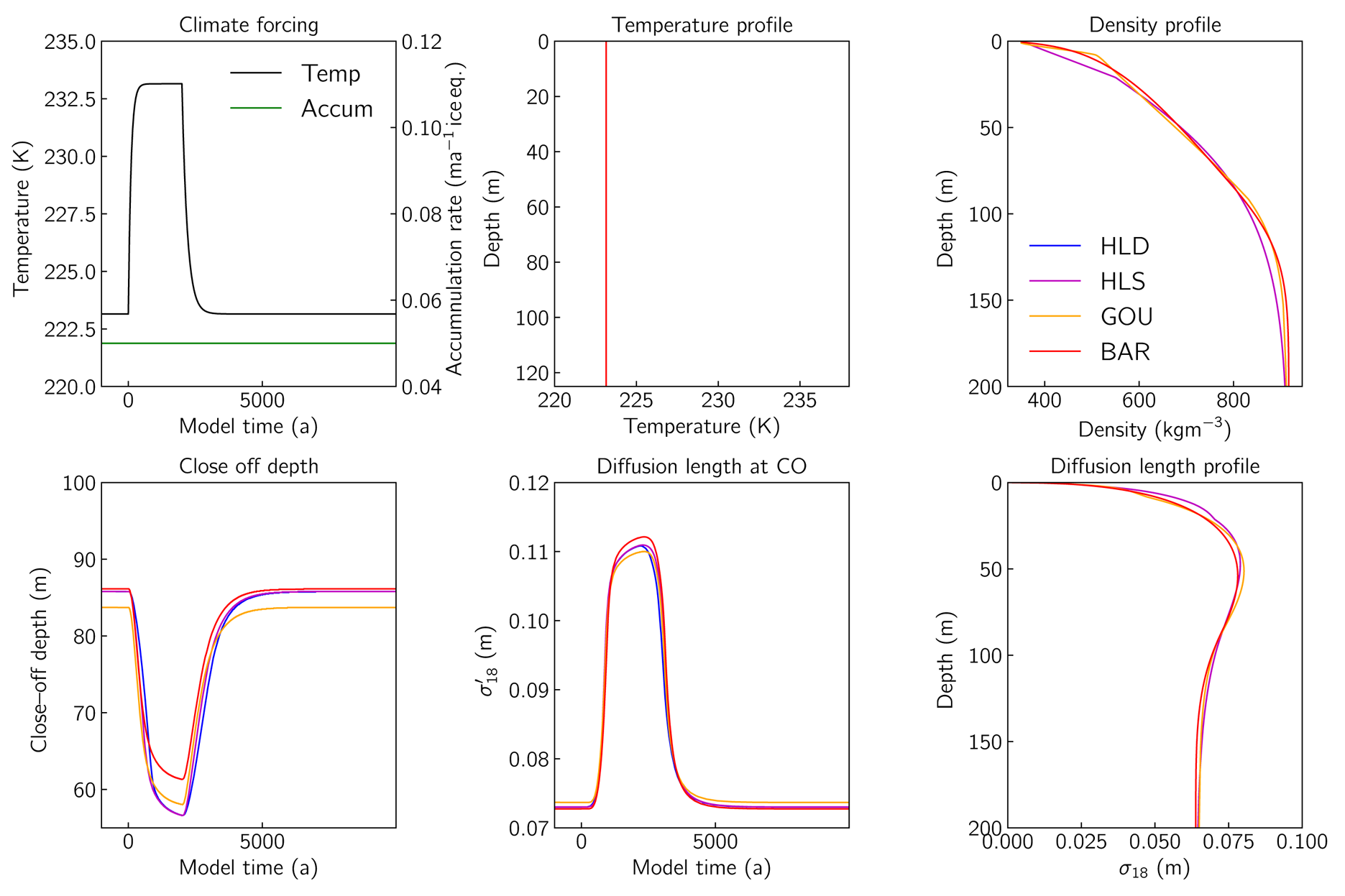
Model comparison for the warming pulse experiments for $\psi = 100\, {\rm years}$ with constant temperature. The vertical profiles (temperature, density and diffusion length) refer to $t = 10\, 000\, {\rm years}$
 .
.

Steady-state type 2 forcing model run with seasonality ON and OFF. The seasonality amplitude is 10 K. (a) Temperature forcing for type 2 steady-state conditions. We plot the last 2 years of the simulation. Each year has a 24 steps resolution. (b) Temperature profile of the firn column with seasonality OFF (red curve) and ON (grey/black lines). We plot the last 24 time steps of the simulation equivalent of 1 year model time. (c) The diffusion length profile comparison.

List of used symbols
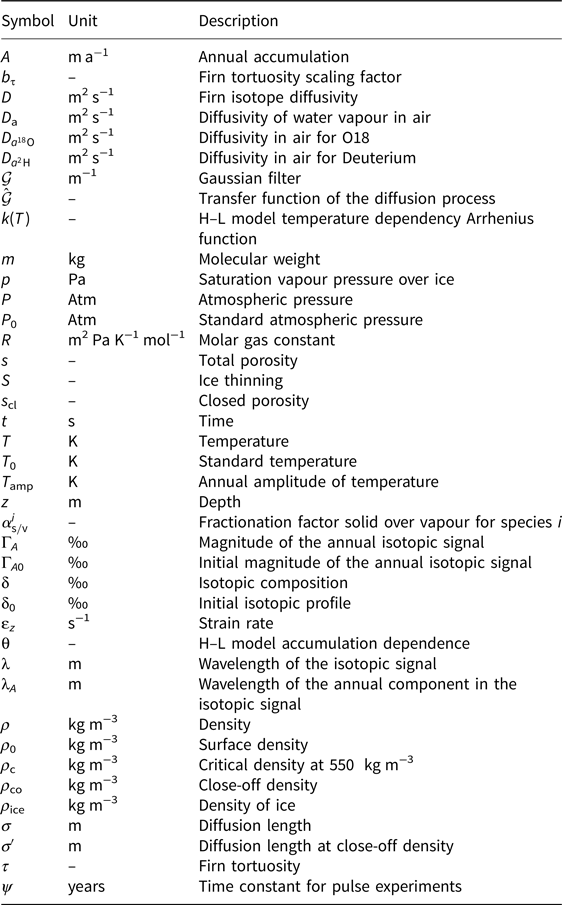


 Open access