

A common and subjective task is classifying objects or subjects, hereafter called items, into predefined, mutually exclusive categories. Examples include content analysis that classifies subjective communications into content categories, meta-analysis that groups empirical studies based on underlying study settings, and medicine that requires appropriate diagnoses of patients. As subsequent analyses and conclusions critically depend on the obtained categorical data, validation is needed. It is, therefore, good practice to assign multiple independent raters and compute the percentage of cases in which these raters chose the same category and thus agreed, where a low percent agreement suggests discarding the data and improving the process. However, researchers also recognized early that this percent agreement is often substantially inflated: It counts not only genuine agreements but also chance agreements in which at least one rater was unsure and coincidently guessed the same category as some other rater, which may happen due to limited choice options. These notions have resulted in chance-corrected agreement coefficients. We provide a review with novel interpretations and connections for so-called quadratic weights.
1 Chance-corrected agreement coefficients
Cohen’s kappa and Scott’s pi are two classic agreement coefficients for two raters (Cohen, Reference Cohen1960; Scott, Reference Scott1955). The chance correction in Cohen’s kappa assumes that raters use their own category proportions (computed from the data) when guessing an item’s category. In contrast, Scott’s pi assumes that the guessing probabilities are the same for both raters by averaging the rater-specific category proportions over the two raters. When extending beyond two raters (i.e., moving to multirater coefficients), Cohen’s kappa generalizes into Conger’s kappa (Conger, Reference Conger1980), and Scott’s pi generalizes into Fleiss’ kappa (Fleiss, Reference Fleiss1971). Both multirater coefficients base the percentage of observed agreement on all items and different rater pairs. However, whereas Conger’s kappa computes the probability of chance agreement by averaging this probability across all rater pairs using rater-specific category proportions, Fleiss’ kappa uses the same (averaged) category proportions for all raters.
Conceptually, the main difference between Scott’s pi and Fleiss’ kappa, on the one hand, and Cohen’s and Conger’s kappas, on the other hand, is that the former two coefficients consider raters to be interchangeable (by averaging the raters’ category proportions), whereas the latter two coefficients do not (Banerjee et al., Reference Banerjee, Capozzoli, McSweeney and Sinha1999; Krippendorff, Reference Krippendorff2004). In addition to Scott’s pi and Fleiss’ kappa, coefficients with interchangeable raters include Krippendorff’s alpha (Krippendorff, Reference Krippendorff2018) and the recently introduced uniform prior coefficient (Van Oest, Reference Van Oest2019; Van Oest & Girard, Reference Van Oest and Girard2022). The latter two coefficients involve traditional versus Bayesian small-sample corrections and converge to Fleiss’ kappa. In the alternative class of noninterchangeable raters, Light’s and Hubert’s kappas complement those of Cohen and Conger (Hubert, Reference Hubert1977; Light, Reference Light1971). Light’s version is the average Cohen’s kappa across all rater pairs (Conger, Reference Conger1980). In contrast, Hubert’s version considers simultaneous agreement among all raters without breaking them up into pairs. It coincides with Conger’s kappa if we measure the degree of simultaneous agreement by the fraction of rater pairs that result in agreement. More generally, the weighted counterparts of these two coefficients coincide if the weight for simultaneous agreement becomes the corresponding average weight across all rater pairs, which is a well-known choice (Mielke et al., Reference Mielke, Berry and Johnston2007, Reference Mielke, Berry and Johnston2009; Schuster & Smith, Reference Schuster and Smith2005; Warrens, Reference Warrens2012a).
Noninterchangeable raters are suitable when all raters classify all items and particularly natural when these raters are fixed (i.e., deliberately selected), such as specific experts, devices, or coding models that constitute the population of interest. In contrast, coefficients with interchangeable raters are needed when raters vary across items (Fleiss, Reference Fleiss1971; Janson & Olsson, Reference Janson and Olsson2004; Landis & Koch, Reference Landis and Koch1977a; Vanbelle, Reference Vanbelle2019). However, the preferred option is less clear-cut when all raters classify all items while being randomly selected to represent a larger population. Zwick (Reference Zwick1988) proposed empirically investigating whether raters vary in category proportions beyond random noise to decide whether raters are interchangeable. A well-known “paradox” of Cohen’s kappa, representing noninterchangeable raters, is that, given the percentage of observed agreement, this kappa increases as raters deviate more in their category proportions, suggesting that rater bias gets rewarded (Feinstein & Cicchetti, Reference Feinstein and Cicchetti1990). However, a counterargument is that the involved ceteris paribus assumption is unrealistic: A change in classification outcomes that triggers additional rater bias typically also decreases the percentage of observed agreement and ultimately Cohen’s kappa, mitigating or even resolving the issue (Hoehler, Reference Hoehler2000).
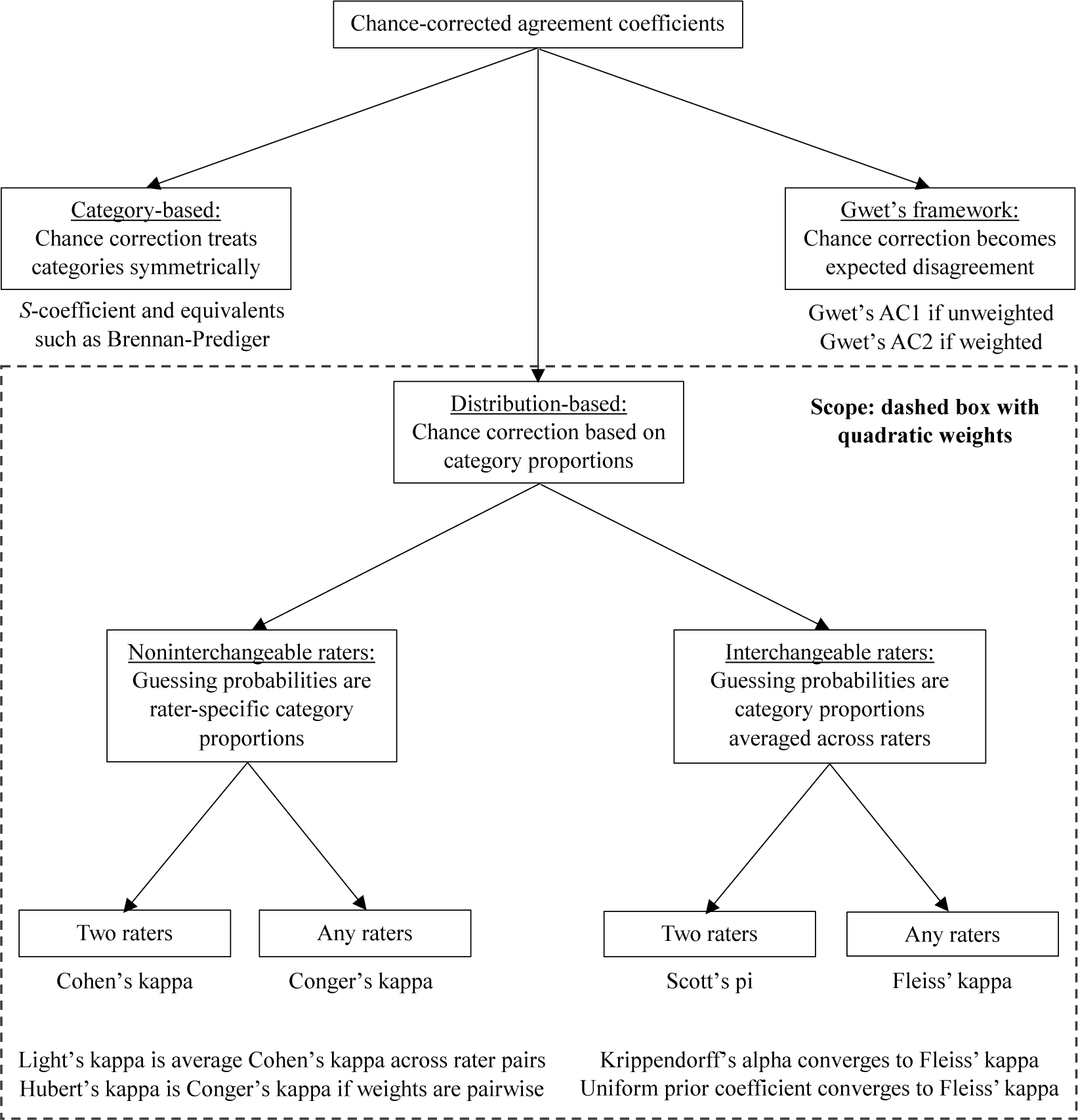
All so-far discussed agreement coefficients are distribution-based, where the chance correction uses raters’ category proportions. An influential alternative class consists of category-based coefficients, where the chance correction uses only information on how many categories and assumes equal category probabilities when raters guess an item’s category. The S-coefficient represents this second class (Bennett et al., Reference Bennett, Alpert and Goldstein1954). Other researchers rediscovered this coefficient via alternative but ultimately equivalent approaches (Brennan & Prediger, Reference Brennan and Prediger1981; Byrt et al., Reference Byrt, Bishop and Carlin1993; Holley & Guilford, Reference Holley and Guilford1964; Janson & Vegelius, Reference Janson and Vegelius1979; Maxwell, Reference Maxwell1977). A third class that has become important is Gwet’s framework, yielding the AC1 and AC2 coefficients (Gwet, Reference Gwet2008, Reference Gwet2014). Figure 1 summarizes all coefficients to guide stakeholders, such as applied researchers, psychometricians, statisticians, and other professionals. The scope of the present study is the distribution-based class, including Cohen’s and Fleiss’ kappas, the most frequently used and cited two-rater and multirater coefficients (e.g., Andres & Hernandez, Reference Andres and Hernandez2020; Vanbelle, Reference Vanbelle2019).
Overview of chance-corrected agreement coefficients plus the scope of the present study.

Figure 1 Long description
A flowchart begins at a top central box labeled Chance-corrected agreement coefficients. Three arrows branch downward from this root.
1. The left branch leads to Category-based: Chance correction treats categories symmetrically. Below this is S-coefficient and equivalents such as Brennan-Prediger.
2. The right branch leads to Gwet's framework: Chance correction becomes expected disagreement. Below this is Gwet's A C 1 if unweighted and Gwet's A C 2 if weighted.
3. The center branch leads into a large dashed box labeled Scope: dashed box with quadratic weights. This branch points to Distribution-based: Chance correction based on category proportions. This node further splits into two sub-branches.
- The left sub-branch is Noninterchangeable raters: Guessing probabilities are rater-specific category proportions. This splits into Two raters leading to Cohen's kappa and Any raters leading to Conger's kappa. Footnotes below state Light's kappa is average Cohen's kappa across rater pairs and Hubert's kappa is Conger's kappa if weights are pairwise.
- The right sub-branch is Interchangeable raters: Guessing probabilities are category proportions averaged across raters. This splits into Two raters leading to Scott's pi and Any raters leading to Fleiss’ kappa. Footnotes below state Krippendorff's alpha converges to Fleiss’ kappa and Uniform prior coefficient converges to Fleiss’ kappa.
A second well-known “paradox” of Cohen’s kappa (i.e., distribution-based coefficients) is that a high observed agreement among raters may still result in a low coefficient value if the categories have substantially unequal proportions (Feinstein & Cicchetti, Reference Feinstein and Cicchetti1990). However, others argued that Cohen’s kappa does what it is supposed to do (Vach, Reference Vach2005; Zwick, Reference Zwick1988). Typically, researchers want raters to agree not only on highly prevalent categories (e.g., not having a disease) but particularly on rare categories (e.g., having that disease). A situation in which raters usually agree on highly prevalent categories but never on rare categories may have serious consequences. However, the percent observed agreement, S-coefficient, and Gwet’s coefficient would take high values. The S-coefficient linearly transforms the observed agreement using only the number of categories without other information (Zwick, Reference Zwick1988); Gwet’s coefficient compares the observed agreement with the corresponding expected disagreement, resulting in higher values as the category proportions become more unequal (Vach & Gerke, Reference Vach and Gerke2023).
2 Incorporating weights for partial disagreements
All coefficients allow for generalization to ordinal (ordered) categories (Cohen, Reference Cohen1968; Gwet, Reference Gwet2014). For example, content analysis may require communication ratings on a five-point scale from very negative (1) to very positive (5). In such situations, some rater disagreements are worse than others, requiring a weighting scheme to describe the amount of penalization for each possible rater disagreement. Typically, exact agreement (i.e., both raters choose the same category) receives a disagreement weight of zero, and the maximum possible disagreement corresponds to a weight of one. All other disagreements receive either the maximum weight of one (reducing to the unweighted case of nominal categories) or a lower distance-based weight, reflecting partial disagreement. Two common weighting schemes are linear and quadratic (Cicchetti & Allison, Reference Cicchetti and Allison1971; Fleiss & Cohen, Reference Fleiss and Cohen1973). The former penalizes rater disagreements in proportion to the distance between the chosen categories; the latter penalizes based on the squared distance. A third, less common, weighting scheme uses radical weights, the distance’s square root (Gwet, Reference Gwet2014). Thus, linear, quadratic, and radical weights penalize disagreements by taking the involved distance (expressed as a fraction of the maximum distance) to the power 1, 2, or 0.5. Quadratic weights are most lenient to partial disagreements and usually yield the highest coefficient values (Van Oest, Reference Van Oest2023; Warrens, Reference Warrens2012b, Reference Warrens2013), potentially explaining their popularity in empirical studies (Vanbelle, Reference Vanbelle2016). However, quadratic weights also offer valuable interpretations as correlation coefficients. All three weighting schemes assume equidistant ordinal categories, where adjacent categories are always the same one point apart. Our results require this well-accepted assumption to hold.
Before turning to quadratic weights, we briefly review existing results for linear weights. First, Cohen’s linearly weighted kappa is a weighted average of kappas computed for all possible reductions of the considered ordinal scale (e.g., five-point) into binary scales by merging adjacent categories (Vanbelle & Albert, Reference Vanbelle and Albert2009; Warrens, Reference Warrens2011). Second, Cohen’s linearly weighted kappa is a weighted average of all linearly weighted kappas computed after merging any two adjacent categories in the ordinal scale, effectively reducing the number of categories by one (Warrens, Reference Warrens2012c). Third, these results generalize to any partition of the ordinal scale by merging adjacent categories: Cohen’s linearly weighted kappa is a weighted average of linearly weighted kappas computed for all possible scale partitions given the chosen number of categories. Furthermore, invariance to the number of categories immediately extends this result to the weighted average across all non-trivial partitions (excluding only the original scale and its reduction to one single category); the weights always correspond to the denominator of the involved kappa elements (Warrens, Reference Warrens2012c). Fourth, Kvålseth (Reference Kvålseth2018) showed that Cohen’s linearly weighted kappa equals the corresponding unweighted kappa if cumulative probabilities replace the original probabilities when computing the latter. Fifth, Cohen’s linearly weighted kappa captures the first moment of the distribution of rating distances generated by the two raters: One minus kappa equals the expected observed rating distance, using the bivariate distribution of ratings, expressed as a fraction of the rating distance that would be expected by chance, under independence (Vanbelle, Reference Vanbelle2016). These results for Cohen’s kappa with linear weights yield elegant decompositions and interpretations, but they do not lead to correlation coefficients.
In contrast, Cohen’s quadratically weighted kappa converges to two-factor intraclass correlation coefficients with random and fixed raters (i.e., the so-called ICC(2,1) and ICC(3,1) coefficients), where the items and raters are the two factors (Carrasco, Reference Carrasco2010; Fleiss & Cohen, Reference Fleiss and Cohen1973; Janson & Olsson, Reference Janson and Olsson2001; Schuster, Reference Schuster2004; Schuster & Smith, Reference Schuster and Smith2005; Shrout & Fleiss, Reference Shrout and Fleiss1979; Warrens, Reference Warrens2014). Furthermore, this kappa coefficient equals Lin’s concordance correlation coefficient (Andres & Hernandez, Reference Andres and Hernandez2020; Carrasco, Reference Carrasco2010; King & Chinchilli, Reference King and Chinchilli2001; Kvålseth, Reference Kvålseth2018; Schuster, Reference Schuster2004). Lin’s concordance correlation possesses several attractive properties and measures agreement (not mere association) between two raters when the ratings are on a continuous scale (Barnhart et al., Reference Barnhart, Haber and Song2002; Lin, Reference Lin1989). In addition, Cohen’s quadratically weighted kappa reduces to the Pearson product–moment correlation if the two raters produced ordinal ratings with the same mean and variance (Brusco et al., Reference Brusco, Stahl and Steinley2008; Cohen, Reference Cohen1968; Schuster, Reference Schuster2004). For Conger’s kappa, the multirater version of Cohen’s kappa, quadratic weights imply convergence to two-factor intraclass correlation coefficients with random and fixed raters, and equivalence to Lin’s generalized concordance correlation coefficient that allows for any number of raters (Andres & Hernandez, Reference Andres and Hernandez2020; Barnhart et al., Reference Barnhart, Haber and Song2002; Carrasco & Jover, Reference Carrasco and Jover2003; Lin, Reference Lin1989, Reference Lin2000; Schuster & Smith, Reference Schuster and Smith2005).
Despite these helpful interpretations, quadratic weights have also received criticism, such as making Cohen’s kappa sensitive to the number of included categories (Brenner & Kliebsch, Reference Brenner and Kliebsch1996), making it behave like a coefficient of association instead of agreement (Graham & Jackson, Reference Graham and Jackson1993), and making it non-responsive to changes in the observed exact agreement on the middle category in situations with an odd number of categories combined with at least one rater having a symmetric distribution of category proportions (Warrens, Reference Warrens2012d).
Although interpretations are abundant for Cohen’s and Conger’s kappas, they are scarce for Fleiss’ kappa, the most frequently used and cited multirater agreement coefficient. Gwet (Reference Gwet2014, p. 67) noted that “there is no known procedure that formally generalizes Scott’s coefficient to Fleiss’,” and Stoyan et al. (Reference Stoyan, Pommerening, Hummel and Kopp-Schneider2018, p. 381) referred to “Fleiss’
$\kappa$
 , which is known to be difficult to interpret.” Still, one existing result is that Fleiss’ kappa converges to the one-factor intraclass correlation coefficient, where the items constitute the only factor due to interchangeable raters (Banerjee et al., Reference Banerjee, Capozzoli, McSweeney and Sinha1999; Janson & Olsson, Reference Janson and Olsson2004; Landis & Koch, Reference Landis and Koch1977a; Vanbelle, Reference Vanbelle2019). Furthermore, a model-based interpretation is that Fleiss’ kappa estimates the probability that both raters in a pair assign an item to its correct category without guessing (Moss, Reference Moss2023; Van Oest, Reference Van Oest2019; Van Oest & Girard, Reference Van Oest and Girard2022). However, interpretations in terms of concordance and Pearson product–moment correlations remain absent.
The present study addresses this literature gap and provides novel interpretations of Fleiss’ quadratically weighted kappa (and its two-rater version, Scott’s pi). We write it as Lin’s generalized concordance correlation coefficient after recentering the raters’ mean vector and covariance matrix at the grand mean to reflect interchangeable raters. Furthermore, Fleiss’ quadratically weighted kappa equals the Pearson product–moment correlation and the regression slope coefficient after concatenating the ratings from all different rater pairs (including reversed rater order) into two data columns. Next, we show a linear connection between Fleiss’ and Conger’s quadratically weighted kappas, entirely determined by the raters’ means and variances, and prove that Fleiss’ quadratically weighted kappa never exceeds Conger’s. The two coefficients coincide if the raters share the same mean rating without needing the same rating proportions or variance. All results extend to Scott’s pi and Cohen’s kappa for two raters with quadratic weights. Thus, we present new interpretations and connections for distribution-based coefficients (see the dashed box in Figure 1).
3 Two noninterchangeable raters: Cohen’s quadratically weighted kappa
To establish ideas, we reproduce that Cohen’s kappa, with quadratic weights, is equivalent to Lin’s bivariate concordance correlation and reduces to the Pearson product–moment correlation if the two raters share the same mean and variance. Cohen’s weighted kappa equals one minus the ratio of observed weighted disagreement,
${d}_o$
 , and expected-by-chance weighted disagreement,
${d}_e$
, and expected-by-chance weighted disagreement,
${d}_e$
 (Cohen, Reference Cohen1968). Expressed in population parameters with
$C$
(Cohen, Reference Cohen1968). Expressed in population parameters with
$C$
 ordered categories, it is

where
$v\left(c,\tilde{c}\right)$
 denotes the disagreement weight when the first rater chooses category
$c$
denotes the disagreement weight when the first rater chooses category
$c$
 and the second rater chooses category
$\tilde{c}$
and the second rater chooses category
$\tilde{c}$
 . Furthermore,
${Y}_1$
. Furthermore,
${Y}_1$
 and
${Y}_2$
and
${Y}_2$
 denote the raters’ category choices (i.e., ratings), with means
${\mu}_1$
denote the raters’ category choices (i.e., ratings), with means
${\mu}_1$
 and
${\mu}_2$
and
${\mu}_2$
 , variances
${\sigma_1}^2$
, variances
${\sigma_1}^2$
 and
${\sigma_2}^2$
and
${\sigma_2}^2$
 , correlation
${\rho}_{1,2}$
, correlation
${\rho}_{1,2}$
 , and covariance
${\sigma}_{1,2}={\rho}_{1,2}{\sigma}_1{\sigma}_2$
, and covariance
${\sigma}_{1,2}={\rho}_{1,2}{\sigma}_1{\sigma}_2$
 . We use quadratic weights and substitute
$v\left(c,\tilde{c}\right)={\left(c-\tilde{c}\right)}^2/{\left(C-1\right)}^2$
. We use quadratic weights and substitute
$v\left(c,\tilde{c}\right)={\left(c-\tilde{c}\right)}^2/{\left(C-1\right)}^2$
 , where the denominator drops out. The numerator and denominator in (1) correspond to the expectations of the weight
$v\left({Y}_1,{Y}_2\right)$
, where the denominator drops out. The numerator and denominator in (1) correspond to the expectations of the weight
$v\left({Y}_1,{Y}_2\right)$
 when considering the joint distribution of
${Y}_1$
when considering the joint distribution of
${Y}_1$
 and
${Y}_2$
and
${Y}_2$
 versus independence:

Using the definition of variance as the second central moment and writing it in terms of the uncentered moments, we can work out (2) as

showing that Cohen’s quadratically weighted kappa coincides with Lin’s bivariate concordance correlation coefficient (Lin, Reference Lin1989). Furthermore, (3) implies that Cohen’s quadratically weighted kappa reduces to the Pearson product–moment correlation
${\rho}_{1,2}$
 if we impose equal means and variances, that is,
${\mu}_1={\mu}_2$
if we impose equal means and variances, that is,
${\mu}_1={\mu}_2$
 and
${\sigma_1}^2={\sigma_2}^2$
and
${\sigma_1}^2={\sigma_2}^2$
 (Cohen, Reference Cohen1968).
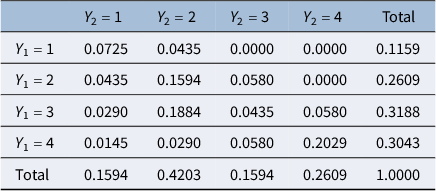
As an illustration, we consider the second contingency table in Table 1 of Landis and Koch (Reference Landis and Koch1977b, p. 161), which compared the multiple sclerosis diagnoses of 69 patients by two neurologists based on four likelihood categories, where “1” is highest and “4” is lowest. Table 1 shows the corresponding joint and marginal distributions.
Joint and marginal distributions of ratings in Landis and Koch’s multiple sclerosis example with two raters

Table 1 Long description
The table consists of 5 rows and 6 columns.
Column Headers:
* The first column is blank.
* Columns 2 through 5 are labeled Y sub 2 = 1, Y sub 2 = 2, Y sub 2 = 3, and Y sub 2 = 4.
* Column 6 is labeled Total.
Row 1 (Y sub 1 = 1):
* Y sub 2 = 1: 0.0725
* Y sub 2 = 2: 0.0435
* Y sub 2 = 3: 0.0000
* Y sub 2 = 4: 0.0000
* Total: 0.1159
Row 2 (Y sub 1 = 2):
* Y sub 2 = 1: 0.0435
* Y sub 2 = 2: 0.1594
* Y sub 2 = 3: 0.0580
* Y sub 2 = 4: 0.0000
* Total: 0.2609
Row 3 (Y sub 1 = 3):
* Y sub 2 = 1: 0.0290
* Y sub 2 = 2: 0.1884
* Y sub 2 = 3: 0.0435
* Y sub 2 = 4: 0.0580
* Total: 0.3188
Row 4 (Y sub 1 = 4):
* Y sub 2 = 1: 0.0145
* Y sub 2 = 2: 0.0290
* Y sub 2 = 3: 0.0580
* Y sub 2 = 4: 0.2029
* Total: 0.3043
Row 5 (Total):
* Y sub 2 = 1: 0.1594
* Y sub 2 = 2: 0.4203
* Y sub 2 = 3: 0.1594
* Y sub 2 = 4: 0.2609
* Total: 1.0000
Cohen’s quadratically weighted kappa equals 0.6256. Furthermore, the raters’ means, variances, and covariance become


and
${\sigma}_{1,2}=0.6780$
 , where we omit the tedious details of the covariance calculation that uses the joint distribution. Lin’s bivariate concordance correlation coefficient is

the same value as Cohen’s quadratically weighted kappa.
4 Two interchangeable raters: Scott’s quadratically weighted pi
We continue with Scott’s pi in the two-rater setting to show how the previous logic for Cohen’s quadratically weighted kappa extends to agreement coefficients with interchangeable raters. Later, we extend to Fleiss’ kappa with any number of interchangeable raters.
4.1 Bivariate concordance correlation after recentering at the raters’ grand mean
Expressed in population parameters with
$C$
 ordered categories, Scott’s pi is

where averaging the marginal category proportions over the two interchangeable raters implies the denominator in (4). Next, incorporating quadratic weights by substituting
$v\left(c,\tilde{c}\right)={\left(c-\tilde{c}\right)}^2$
 , recognizing the numerator in (4) as the expectation of the weight
$v\left({Y}_1,{Y}_2\right)$
, recognizing the numerator in (4) as the expectation of the weight
$v\left({Y}_1,{Y}_2\right)$
 when considering the joint distribution of
${Y}_1$
when considering the joint distribution of
${Y}_1$
 and
${Y}_2$
and
${Y}_2$
 , and recognizing independence in the denominator yields

where

with
${\tilde{Y}}_1$
 and
${\tilde{Y}}_2$
and
${\tilde{Y}}_2$
 originating from the same distributions as
${Y}_1$
originating from the same distributions as
${Y}_1$
 and
${Y}_2$
and
${Y}_2$
 , respectively. Substituting (6) into (5) yields a new expression for Scott’s pi in terms of the first and second moments:

Furthermore, (7) implies that Scott’s pi with quadratic weights reduces to the Pearson product–moment correlation
${\rho}_{1,2}$
 if we impose equal means and variances, that is,
${\mu}_1={\mu}_2$
if we impose equal means and variances, that is,
${\mu}_1={\mu}_2$
 and
${\sigma_1}^2={\sigma_2}^2$
and
${\sigma_1}^2={\sigma_2}^2$
 .
.
Comparing expressions (3) and (7) for Cohen’s quadratically weighted kappa and the corresponding Scott’s pi shows that these coefficients coincide if the two raters share the same mean,
${\mu}_1={\mu}_2$
 . This requirement of equal rater means is substantially more relaxed than the typical requirement of raters having the same category proportions for the unweighted kappa and pi coefficients. For example, Banerjee et al. (Reference Banerjee, Capozzoli, McSweeney and Sinha1999, p. 5) noted for nominal categories that “if the two raters are interchangeable, in the sense that the marginal distributions are identical, then Cohen’s and Scott’s measures are equivalent.” In contrast, when the weights are quadratic, having the same mean is already sufficient for interchangeability, making these coefficients equivalent.
Next, we rewrite Scott’s pi in (7) as

where
${\tilde{\sigma}}_{1,2}={\sigma}_{1,2}+{\mu}_1{\mu}_2-{\overline{\mu}}^2$
 is the covariance after recentering the rater means,
${\mu}_1$
is the covariance after recentering the rater means,
${\mu}_1$
 and
${\mu}_2$
and
${\mu}_2$
 , at the grand mean,
$\overline{\mu}=\left({\mu}_1+{\mu}_2\right)/2$
, at the grand mean,
$\overline{\mu}=\left({\mu}_1+{\mu}_2\right)/2$
 , and
${{\tilde{\sigma}}_1}^2$
, and
${{\tilde{\sigma}}_1}^2$
 and
${{\tilde{\sigma}}_2}^2$
and
${{\tilde{\sigma}}_2}^2$
 are the corresponding recentered variances. Thus, we may interpret Cohen’s quadratically weighted kappa in (3) and Scott’s quadratically weighted pi in (7) as concordance correlation coefficients, where the interchangeable raters in Scott’s pi imply recentering the rater means and (co)variances at the grand mean.
4.2 Pearson correlation and regression slope after concatenating the ratings
Another interpretation of Scott’s quadratically weighted pi is that it equals the Pearson product–moment correlation when the order of the two raters is random, with each of the two possible rater pairs, (1,2) and (2,1), occurring with 50% probability. Since the rater order is random, the two raters in the pair become random and effectively interchangeable with the same mean and variance. Following earlier logic, using equal means and variances, and denoting the two random raters as
${J}_1$
 and
${J}_2$
and
${J}_2$
 , we indeed obtain that Scott’s pi is the corresponding Pearson correlation:

In practice, researchers can compute Scott’s quadratically weighted pi by computing the Pearson correlation after concatenating the data, that is, combining the ratings from the two possible rater pairs, (1,2) and (2,1), in one extended data set with twice as many ratings. This procedure starts from the original contingency table, containing the rating frequencies of the two raters, and adds the transpose of this contingency table, making the combined contingency table symmetric. As the raters always become interchangeable after combining the two possible rater orders, it does not matter whether the same two raters rated all items or raters varied across items. However, the variance (and standard error) of this Pearson correlation is invalid because the ratings of the flipped rater pair are a direct consequence of the original ratings, violating the requirement of being drawn independently from the same data-generating process. Gwet (Reference Gwet2014, p. 141) and Andres and Hernandez (Reference Andres and Hernandez2025) provided formulas to compute the correct variance of Scott’s pi for fixed raters. Furthermore, Gwet (Reference Gwet2014) proposed an additive jackknife variance component if the raters are random (i.e., the participating raters are not of central interest and instead drawn from a larger population they are supposed to represent).
Next, we note that (9) implies
$\pi =\beta$
 , where
$\beta$
, where
$\beta$
 is the slope in
${Y}_{J_2}=\alpha +\beta {Y}_{J_1}+\varepsilon$
is the slope in
${Y}_{J_2}=\alpha +\beta {Y}_{J_1}+\varepsilon$
 . The reason is that the slope coefficient in a simple linear regression equals the covariance between the independent variable and the dependent variable divided by the variance of the independent variable, that is,
$\beta =\mathrm{Cov}\left[{Y}_{J_1},{Y}_{J_2}\right]/\mathrm{Var}\left[{Y}_{J_1}\right]$
. The reason is that the slope coefficient in a simple linear regression equals the covariance between the independent variable and the dependent variable divided by the variance of the independent variable, that is,
$\beta =\mathrm{Cov}\left[{Y}_{J_1},{Y}_{J_2}\right]/\mathrm{Var}\left[{Y}_{J_1}\right]$
 (e.g., Wooldridge, Reference Wooldridge2012, p. 29). Thus, analogous to before, researchers can compute Scott’s quadratically weighted pi by estimating the slope coefficient in a simple linear regression for the concatenated ratings of rater pairs (1,2) and (2,1). However, standard regression theory no longer helps obtain the corresponding variance.
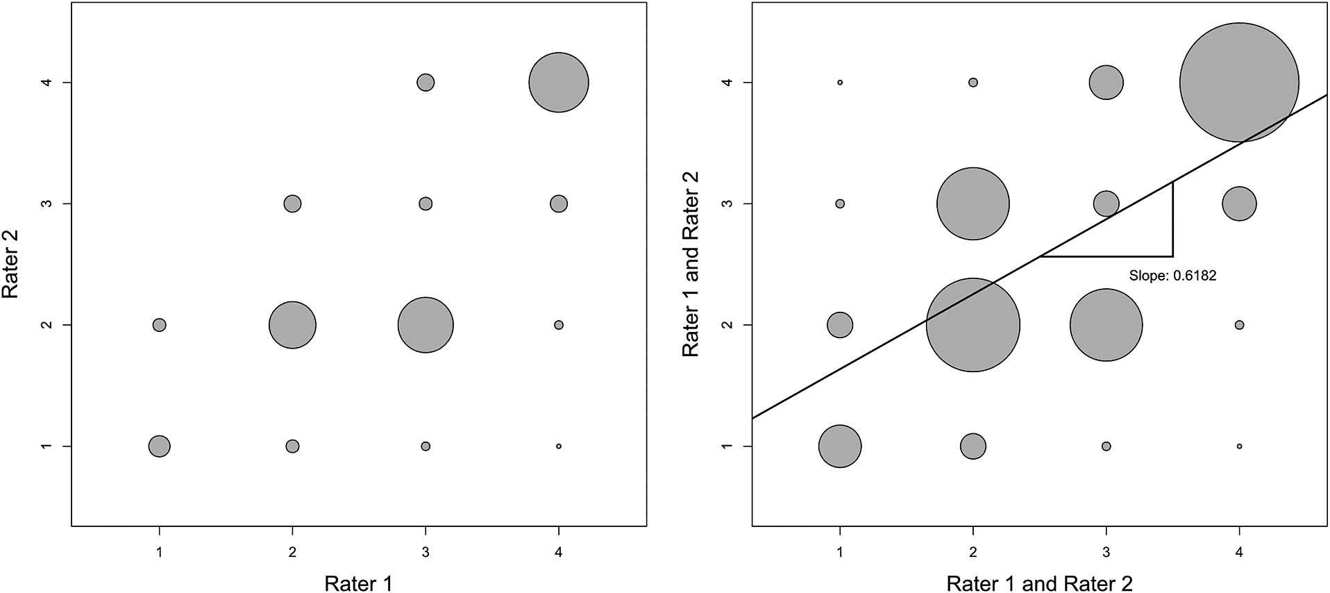
Moving from the left to the right panel in Figure 2 shows how the concatenation works in the multiple sclerosis example of Landis and Koch (Reference Landis and Koch1977b). For each cell, we sum the original rating frequency of the rater pair (1,2) and the diagonal-mirrored frequency of the flipped rater pair (2,1). Fleiss’ kappa equals the Pearson correlation and regression slope in the figure’s right panel.
After concatenation, Scott’s quadratically weighted pi equals the Pearson correlation and regression slope of 0.6182 in Landis and Koch’s two-rater multiple sclerosis example. Scatter plot of original frequencies (left) and combined frequencies with regression line (right).

Figure 2 Long description
Two panels show bubble scatter plots where the size of each circle represents frequency.
* Left Panel: The x axis is labeled Rater 1 and the y axis is labeled Rater 2, both with scales from 1 to 4. Bubbles are distributed across the grid. The largest bubble is at the coordinate (4, 4). Medium-sized bubbles are located at (2, 2) and (3, 2). Smaller bubbles are scattered at other integer intersections.
* Right Panel: Both axes are labeled Rater 1 and Rater 2. This panel shows combined frequencies. A solid black regression line rises diagonally from left to right. A right-angle triangle is drawn under the line to indicate the slope, with the text Slope: 0.6182. The largest bubbles are concentrated along the diagonal at (4, 4), (2, 3), (2, 2), and (3, 2). Smaller bubbles appear at off-diagonal positions such as (1, 1), (1, 2), (3, 3), and (4, 3).
4.3 Linear function of Cohen’s quadratically weighted kappa
We write Scott’s quadratically weighted pi in (7) as a linear function of Cohen’s quadratically weighted kappa in (3), conditional on the rater means and variances (Appendix A):

where

is the squared difference in rater means divided by the corresponding variance under independence. Its sample counterpart is related to the Wald (or squared t) statistic to test for equal means while allowing for unequal variances. Equation (10) shows that Scott’s pi cannot exceed Cohen’s kappa, so the latter coefficient provides an upper bound for the former. Whereas Warrens (Reference Warrens2010a) proved this result for nominal weights, we demonstrate it for quadratic weights.
Although Scott’s quadratically weighted pi is a linear function of Cohen’s quadratically weighted kappa conditional on the rater means and variances, the relationship between the variance estimators of these coefficients remains complex. The reason is that both the coefficients and rater moments are functions of the data and interact nonlinearly in (10) and (11).
4.4 Numerical example
Continuing with the multiple sclerosis example of Landis and Koch (Reference Landis and Koch1977b, p. 161), we use (7) to compute Scott’s quadratically weighted pi as

Next, we use (8) to compute Scott’s pi as Lin’s concordance correlation coefficient after recentering at the raters’ grand mean, which is
$\overline{\mu}=\left(2.8116+2.5217\right)/2=2.6667$
 :
:

yielding the same coefficient value.
We proceed by computing Scott’s quadratically weighted pi as the Pearson product–moment correlation and the regression slope after concatenating the ratings of the original rater pair (1,2) and flipped rater pair (2,1), that is, adding the transposed contingency table to the original one. The correlation and slope coefficients become the covariance divided by the variance (where the two data columns share the same mean and variance after concatenation). The R-code below starts from Landis and Koch’s
$4\times 4$
 contingency table and avoids translating this contingency table into item-by-rater tables of ratings. It again yields a value of 0.6182:
y <- matrix(c(5,3,2,1,3,11,13,2,0,4,3,4,0,0,4,14),nrow=4)
y <- (y+t(y))/(2*sum(y))
mean <- sum(1:nrow(y)*rowSums(y))
var <- sum((1:nrow(y))^2*rowSums(y))-mean^2
cov <- sum(outer(1:nrow(y),1:nrow(y))*y)-mean^2
cov/var
[1] 0.6181818
Furthermore, Scott’s quadratically weighted pi is a linear function of Cohen’s quadratically weighted kappa (and vice versa), with the intercept and slope solely depending on the squared difference in means divided by the corresponding variance under independence:

Substituting into (10) yields

5 Any noninterchangeable raters: Conger’s quadratically weighted kappa
To explain how the previous ideas extend to multirater coefficients with more than two raters, we show that Conger’s quadratically weighted kappa equals Lin’s generalized concordance correlation coefficient and reduces to the average Pearson product–moment correlation across all rater pairs if raters share the same mean and variance. This proof is shorter and less complex than found elsewhere in the literature (Andres & Hernandez, Reference Andres and Hernandez2020; Schuster & Smith, Reference Schuster and Smith2005; Warrens, Reference Warrens2012a); the result for the average Pearson correlation is new. Later, we extend to the more complex analysis of Fleiss’ quadratically weighted kappa with interchangeable raters.
We denote Conger’s quadratically weighted kappa for
$R$
 raters as
${\kappa}_C$
raters as
${\kappa}_C$
 to distinguish it from Cohen’s
$\kappa$
to distinguish it from Cohen’s
$\kappa$
 for two raters. In Conger’s kappa, both the observed disagreement,
${d}_o$
for two raters. In Conger’s kappa, both the observed disagreement,
${d}_o$
 , and expected disagreement,
${d}_e$
, and expected disagreement,
${d}_e$
 , are averages (or equivalently, sums) across all pairs of different raters
$\left(r,\tilde{r}\right)$
, are averages (or equivalently, sums) across all pairs of different raters
$\left(r,\tilde{r}\right)$
 with
$\tilde{r}>r$
with
$\tilde{r}>r$
 (Conger, Reference Conger1980):

Recognizing the expectations in square brackets, with independence in the denominator, yields

Next, we use that
${\sum}_{r=1}^{R-1}{\sum}_{\tilde{r}>r}\left({\sigma_r}^2+{\sigma_{\tilde{r}}}^2\right)=\left(R-1\right){\sum}_{r=1}^R{\sigma_r}^2$
 and simplify (14) to obtain Lin’s generalized concordance correlation coefficient, suitable for any number of raters (Andres & Hernandez, Reference Andres and Hernandez2020; Barnhart et al., Reference Barnhart, Haber and Song2002; Carrasco & Jover, Reference Carrasco and Jover2003; Lin, Reference Lin1989, Reference Lin2000):

We note that (15) reduces to Cohen’s quadratically weighted kappa and the bivariate concordance correlation coefficient in (3) if there are only two raters, with
$R=2$
 .
.
Conger’s kappa in (15) becomes the average Pearson product–moment correlation across all rater pairs if raters share the same mean and the same variance,
${\sigma}^2$
 :
:

Finally, we express (15) in matrix and vector notation for convenient coding in matrix programming languages:

where
$^{\prime }$
 denotes the transpose,
$\iota$
denotes the transpose,
$\iota$
 is the R-dimensional vector of ones,
$\Sigma =\left({\sigma}_{r,\tilde{r}}\right)$
is the R-dimensional vector of ones,
$\Sigma =\left({\sigma}_{r,\tilde{r}}\right)$
 is the covariance matrix, “tr” is the trace (i.e., sum of diagonal elements),
$\overline{\mu}={\iota}^{\prime}\mu /R$
is the covariance matrix, “tr” is the trace (i.e., sum of diagonal elements),
$\overline{\mu}={\iota}^{\prime}\mu /R$
 , and
$\overline{\mu^2}=\iota^{\prime }{\mu}^2/R$
, and
$\overline{\mu^2}=\iota^{\prime }{\mu}^2/R$
 , with
$\mu$
, with
$\mu$
 and
${\mu}^2$
and
${\mu}^2$
 being R-dimensional vectors containing the rater means and squared rater means. Comparing (17) with the matrix expressions in Almehrizi and Emam (Reference Almehrizi and Emam2023) reveals identical numerators and related denominators. Their two-factor intraclass correlation coefficient for absolute agreement (labeled
${\rho}_{\left(A,1\right)}$
being R-dimensional vectors containing the rater means and squared rater means. Comparing (17) with the matrix expressions in Almehrizi and Emam (Reference Almehrizi and Emam2023) reveals identical numerators and related denominators. Their two-factor intraclass correlation coefficient for absolute agreement (labeled
${\rho}_{\left(A,1\right)}$
 ) converges to Conger’s quadratically weighted kappa in (17), as their only deviating term converges to
$\left(R-1\right)\mathrm{tr}\left(\Sigma \right)$
) converges to Conger’s quadratically weighted kappa in (17), as their only deviating term converges to
$\left(R-1\right)\mathrm{tr}\left(\Sigma \right)$
 . Furthermore, the term
${R}^2\left(\overline{\mu^2}-{\left(\overline{\mu}\right)}^2\right)$
. Furthermore, the term
${R}^2\left(\overline{\mu^2}-{\left(\overline{\mu}\right)}^2\right)$
 is absent in their two-factor intraclass correlation coefficient for relative consistency (labeled
${\rho}_{\left(C,1\right)}$
is absent in their two-factor intraclass correlation coefficient for relative consistency (labeled
${\rho}_{\left(C,1\right)}$
 ). Hence, this coefficient coincides with Conger’s kappa in (17) if all raters share the same mean.
As an illustration, we consider Table A.3 of Gwet (Reference Gwet2014, p. 371), showing the five-point color intensity ratings of 29 stickleback fishes by four experienced raters. Based on maximum likelihood estimation, these raters have the following mean vector and covariance matrix:

implying that
${\iota}^{\prime}\Sigma \iota =30.5470$
 ,
$\mathrm{tr}\left(\Sigma \right)=9.5125$
,
$\mathrm{tr}\left(\Sigma \right)=9.5125$
 ,
$\overline{\mu}=2.7672$
,
$\overline{\mu}=2.7672$
 , and
$\overline{\mu^2}=7.6650$
, and
$\overline{\mu^2}=7.6650$
 . Plugging these numbers into (17) yields the value of Conger’s quadratically weighted kappa and the generalized concordance correlation coefficient, which is also the value reported in Gwet (Reference Gwet2014, p. 158):

Letting y denote the 29 × 4 item-by-rater data matrix from Gwet (Reference Gwet2014, p. 371), then coding up (17) in R is straightforward and yields the same coefficient value:
R <- ncol(y)
mu <- colMeans(y)
Sigma <- cov(y)*((nrow(y)-1)/nrow(y)) # ML estimation
num <- sum(Sigma)-sum(diag(Sigma))
den <- (R-1)*sum(diag(Sigma))+(R^2)*(mean(mu^2)-(mean(mu))^2)
num/den
[1] 0.7340554
In all remaining programming codes, we will refer to the data matrix as y and skip the calculations of
$R$
 (i.e., number of raters),
$\unicode{x3bc}$
(i.e., number of raters),
$\unicode{x3bc}$
 , and
$\Sigma$
, and
$\Sigma$
 because these calculations remain identical.
6 Any interchangeable raters: Fleiss’ quadratically weighted kappa
We turn to the coefficient of primary interest, Fleiss’ quadratically weighted kappa with any number of interchangeable raters, denoted as
${\kappa}_F$
 . These results are new.
6.1 Generalized concordance correlation after recentering at the raters’ grand mean
Fleiss’ kappa computes the observed disagreement,
${d}_o$
 , in the same way as Conger’s: It takes the corresponding average over all pairs of different raters. However, unlike Conger’s kappa, Fleiss’ chance correction aggregates the category proportions across raters and uses these average proportions to compute its expected disagreement,
${d}_e$
, in the same way as Conger’s: It takes the corresponding average over all pairs of different raters. However, unlike Conger’s kappa, Fleiss’ chance correction aggregates the category proportions across raters and uses these average proportions to compute its expected disagreement,
${d}_e$
 (Fleiss, Reference Fleiss1971):

Using that
${R}^2/\left(\begin{array}{c}R\\ {}2\end{array}\right)=2R/\left(R-1\right)$
 and recognizing the expectations, we can write (18) as

Next, we break up the summations in the denominator into
$r=\tilde{r}$
 ,
$r<\tilde{r}$
,
$r<\tilde{r}$
 , and symmetric
$r>\tilde{r}$
, and symmetric
$r>\tilde{r}$
 :
:

Finally, we divide the numerator and denominator by two, use that
${\sum}_{r=1}^{R-1}{\sum}_{\tilde{r}>r}\left({\sigma_r}^2+{\sigma_{\tilde{r}}}^2\right)=\left(R-1\right){\sum}_{r=1}^R{\sigma_r}^2$
 , and simplify to obtain

Using the same matrix and vector notation as before, this expression for Fleiss’ quadratically weighted kappa becomes

We note that (21) reduces to Scott’s quadratically weighted pi in (7) if there are only two raters, with
$R=2$
 . Furthermore, it becomes the average Pearson product–moment correlation across all rater pairs if raters share the same mean and the same variance,
${\sigma}^2$
. Furthermore, it becomes the average Pearson product–moment correlation across all rater pairs if raters share the same mean and the same variance,
${\sigma}^2$
 :
:

Comparing expressions (15) and (21) for Conger’s and Fleiss’ quadratically weighted kappas shows that these coefficients coincide if all raters share the same mean, which is a much less stringent condition than all raters having identical category proportions (i.e., the same marginal distributions).
Next, we show that Fleiss’ quadratically weighted kappa in (21) equals Lin’s generalized concordance correlation coefficient after recentering the rater means and covariance matrix at the raters’ grand mean (Appendix B):

where
${\tilde{\sigma}}_{r,\tilde{r}}={\sigma}_{r,\tilde{r}}+{\mu}_r{\mu}_{\tilde{r}}-{\overline{\mu}}^2$
 denotes the covariances after recentering at
$\overline{\mu}={\sum}_{r=1}^R{\mu}_r/R$
denotes the covariances after recentering at
$\overline{\mu}={\sum}_{r=1}^R{\mu}_r/R$
 and
${{\tilde{\sigma}}_r}^2={\sigma_r}^2+{\mu_r}^2-{\overline{\mu}}^2$
and
${{\tilde{\sigma}}_r}^2={\sigma_r}^2+{\mu_r}^2-{\overline{\mu}}^2$
 denotes the recentered variances. Using the same matrix and vector notation as before, the recentered covariance matrix becomes
$\tilde{\Sigma}=\Sigma +\mu {\mu}^{\prime }-{\overline{\mu}}^2$
denotes the recentered variances. Using the same matrix and vector notation as before, the recentered covariance matrix becomes
$\tilde{\Sigma}=\Sigma +\mu {\mu}^{\prime }-{\overline{\mu}}^2$
 . This result generalizes an earlier result, obtained in (8) for Scott’s pi with two raters, to any number of raters.
6.2 Pearson correlation and regression slope after concatenating the ratings
Fleiss’ quadratically weighted kappa is the multirater generalization of the corresponding Scott’s pi. As Scott’s pi equals the Pearson product–moment correlation between the ratings from two random, different raters, Fleiss’ kappa has the same interpretation. Treating the two raters in the pair as random makes these raters interchangeable with the same mean and variance, so the same proof as in (9) applies. In practice, researchers can compute Fleiss’ kappa with quadratic weights by appropriately concatenating the data and then computing the Pearson correlation from these concatenated ratings. The concatenation procedure generalizes the approach for Scott’s pi. It combines the ratings from all possible rater pairs (including the same pair after flipping the two raters) in a new data set, where the first column captures the first rater in the pair, and the second column captures the second rater. For example, for three raters, the two data columns combine (i.e., concatenate) the ratings from the six rater pairs (1,2), (2,1), (1,3), (3,1), (2,3), and (3,2).
Furthermore, analogous to before, researchers can compute the value of Fleiss’ quadratically weighted kappa by estimating the slope coefficient in a simple linear regression, where the two data columns with concatenated ratings serve as dependent and independent variables (or vice versa). However, standard statistical theory no longer helps obtain the variances, as the concatenated ratings are no independent draws from the data-generating process. We refer to other literature sources to get the correct variance of Fleiss’ kappa (Andres & Hernandez, Reference Andres and Hernandez2025; Gwet, Reference Gwet2014; Schouten, Reference Schouten1980, Reference Schouten1982; Vanbelle, Reference Vanbelle2019). Furthermore, a high-quality R package to compute agreement coefficients and their variances is irrCAC.
6.3 Linear function of Conger’s quadratically weighted kappa
Generalizing the result in (10) for two raters to any number of raters, we write Fleiss’ quadratically weighted kappa in (21) as a linear function of Conger’s quadratically weighted kappa in (15), conditional on the rater means and variances (Appendix C):

where

is the sum of squared differences in means across all rater pairs divided by the corresponding sum of variances under independence. We recall
${\sum}_{r=1}^{R-1}{\sum}_{\tilde{r}>r}\left({\sigma_r}^2+{\sigma_{\tilde{r}}}^2\right)=\left(R-1\right){\sum}_{r=1}^R{\sigma_r}^2$
 . Equation (25) shows that Fleiss’ quadratically weighted kappa cannot exceed Conger’s, implying that the latter coefficient provides an upper bound for the former. Whereas Warrens (Reference Warrens2010b) proved this result for nominal weights, we extend it to quadratic weights. Furthermore, (25) provides an alternative proof that Conger’s and Fleiss’ quadratically weighted kappas converge to each other as the number of raters,
$R$
. Equation (25) shows that Fleiss’ quadratically weighted kappa cannot exceed Conger’s, implying that the latter coefficient provides an upper bound for the former. Whereas Warrens (Reference Warrens2010b) proved this result for nominal weights, we extend it to quadratic weights. Furthermore, (25) provides an alternative proof that Conger’s and Fleiss’ quadratically weighted kappas converge to each other as the number of raters,
$R$
 , tends to infinity (Conger, Reference Conger1980; Gwet, Reference Gwet2014).
Although Fleiss’ quadratically weighted kappa is a linear function of Conger’s quadratically weighted kappa conditional on the rater means and variances, the relationship between the variance estimators of these kappas remains complex. The reason is that both the kappas and rater moments are functions of the data and interact nonlinearly in (25) and (26).
6.4 Numerical example
Continuing with the four-rater stickleback fish color example of Gwet (Reference Gwet2014, p. 371) and using our earlier calculations of
${\iota}^{\prime}\Sigma \iota =30.5470$
 ,
$\mathrm{tr}\left(\Sigma \right)=9.5125$
,
$\mathrm{tr}\left(\Sigma \right)=9.5125$
 ,
$\overline{\mu}=2.7672$
,
$\overline{\mu}=2.7672$
 , and
$\overline{\mu^2}=7.6650$
, and
$\overline{\mu^2}=7.6650$
 , we plug these numbers into (22) to compute Fleiss’ quadratically weighted kappa as

which is also the value reported in Gwet (Reference Gwet2014, p. 158). As the four raters have almost the same mean rating (only the second rater deviates somewhat), it is unsurprising that the values of Conger’s and Fleiss’ kappas are virtually identical (0.7341 vs. 0.7338). Indeed, we identified equal rater means as a sufficient condition for these two coefficients, with quadratic weights, to coincide.
We may also compute Fleiss’ quadratically weighted kappa as Lins’ generalized concordance correlation coefficient after recentering at the raters’ grand mean, resulting in the transformed covariance matrix:

where
${\iota}^{\prime}\tilde{\Sigma}\iota =30.5470$
 and
$\mathrm{tr}\left(\tilde{\Sigma}\right)=9.5419$
and
$\mathrm{tr}\left(\tilde{\Sigma}\right)=9.5419$
 . Continuing with matrix and vector notation and substituting into (24) yields the same coefficient value as above:

Coding up Fleiss’ quadratically weighted kappa using the rater means and covariance matrix via (22) and as a generalized concordance correlation via (24) yields the same results:
num <- sum(Sigma)-sum(diag(Sigma))-R*(mean(mu^2)-(mean(mu))^2)
den <- (R-1)*sum(diag(Sigma))+R*(R-1)*(mean(mu^2)-(mean(mu))^2)
num/den
[1] 0.7337819
and
Sigma_tilde <- Sigma+outer(mu,mu)-(mean(mu))^2
num <- sum(Sigma_tilde)-sum(diag(Sigma_tilde))
den <- (R-1)*sum(diag(Sigma_tilde))
num/den
[1] 0.7337819
Furthermore, Fleiss’ quadratically weighted kappa is a linear function of Conger’s quadratically weighted kappa (and vice versa). Plugging the numbers into (26) yields

and substituting into (25) yields


Coding up this linear connection in R, starting from
${\kappa}_C=0.7340554$
 , yields the correct
${\kappa}_F$
, yields the correct
${\kappa}_F$
 :
:
kappa_C <- 0.7340554
W <- (R^2)*(mean(mu^2)-(mean(mu))^2)/((R-1)*sum(diag(Sigma)))
kappa_C-(W/(R+(R-1)*W))*(1-kappa_C)
[1] 0.733782
Finally, we show how researchers can compute Fleiss’ quadratically weighted kappa as either the Pearson product–moment correlation or the regression slope after appropriately concatenating the ratings into two columns. Since we have four raters, we combine the ratings from 12 rater pairs: (1,2), (1,3), (1,4), (2,3), (2,4), (3,4), (2,1), (3,1), (4,1), (3,2), (4,2), and (4,3), where we may list these pairs in any possible order. The R code for the Pearson correlation of the concatenated ratings is as follows:
y1 <- c(y[,1],y[,1],y[,1],y[,2],y[,2],y[,3])
y2 <- c(y[,2],y[,3],y[,4],y[,3],y[,4],y[,4])
cor(c(y1,y2),c(y2,y1))
[1] 0.7337819
We can also run the corresponding simple linear regression and inspect the slope:
unname(coef(lm(c(y1,y2)~c(y2,y1)))[2])
[1] 0.7337819
7 Discussion
We provided a review of distribution-based agreement coefficients with quadratic weights. This extensive class includes the most frequently used and cited coefficients in the literature: Cohen’s kappa for two raters and Fleiss’ kappa for more than two raters. Furthermore, quadratic weights are the most common in empirical studies (Vanbelle, Reference Vanbelle2016; Warrens, Reference Warrens2014). These weights possess the attractive property that many distribution-based coefficients become correlation coefficients, facilitating interpretation. Figure 3 provides an overview. In addition to four classic agreement coefficients (i.e., Scott’s pi, Cohen’s, Conger’s, and Fleiss’ kappas), the correlation interpretations extend to other multirater coefficients. Light’s kappa is the average of all pairwise Cohen’s kappas. Hubert’s kappa defines rater (dis)agreements by the joint outcome of all
$R$
 raters; it becomes Conger’s kappa if the
$R$
raters; it becomes Conger’s kappa if the
$R$
 -rater weight is the corresponding average weight across all rater pairs, which is a well-documented choice (Andres & Hernandez, Reference Andres and Hernandez2020; Mielke et al., Reference Mielke, Berry and Johnston2007, Reference Mielke, Berry and Johnston2009; Schuster & Smith, Reference Schuster and Smith2005; Warrens, Reference Warrens2012a). Krippendorff’s alpha and the recently introduced uniform prior coefficient involve traditional versus Bayesian small-sample corrections and converge to Fleiss’ kappa. The interpretations for interchangeable raters in the right half of Figure 3 are new. Some of these results extend existing interpretations to interchangeable raters. Other results are unique, such as the Pearson correlation and regression slope after concatenating all rater pairs (including reversed rater order). Most interpretations for noninterchangeable raters in the left half of Figure 3 already exist in the literature.
Correlation interpretations of distribution-based agreement coefficients with quadratic weights.

Figure 3 Long description
A flowchart begins at a top central box titled Distribution-based agreement coefficients with quadratic weights. Two arrows point downward to two distinct categories.
Left branch: Noninterchangeable raters. This column lists four primary coefficients with their interpretations:
1. Cohen's kappa (two raters): Includes Intraclass correlation if many items, Bivariate concordance correlation, and Pearson correlation if equal rater means and variances.
2. Conger's kappa (any raters): Includes Intraclass correlation if many items, Generalized concordance correlation, and Average Pearson correlation across all rater pairs if equal rater means and variances.
3. Light's kappa (any raters): Includes Average intraclass correlation across all rater pairs if many items, Average bivariate concordance correlation across all rater pairs, and Average Pearson correlation across all rater pairs if equal rater means and variances.
4. Hubert's kappa with pairwise weights (any raters): Includes Intraclass correlation if many items, Generalized concordance correlation, and Average Pearson correlation across all rater pairs if equal rater means and variances.
Right branch: Interchangeable raters. This column lists four primary coefficients with their interpretations:
1. Scott's pi (two raters): Includes Bivariate concordance correlation after recentering rater means and covariance matrix at grand mean, Pearson correlation if equal rater means and variances, Pearson correlation for concatenated ratings of rater pair and flipped rater pair, and Regression slope for concatenated ratings of rater pair and flipped rater pair.
2. Fleiss’ kappa (any raters): Includes Generalized concordance correlation after recentering rater means and covariance matrix at grand mean, Average Pearson correlation across all rater pairs if equal rater means and variances, Pearson correlation for concatenated ratings of all rater pairs including flipped rater order, and Regression slope for concatenated ratings of all rater pairs including flipped rater order.
3. Krippendorff's alpha with many items (any raters): Lists the same four interpretations as Fleiss’ kappa.
4. Uniform prior coefficient with many items (any raters): Lists the same four interpretations as Fleiss’ kappa.
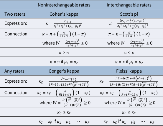
Table 2 shows the connections between quadratically weighted agreement coefficients that assume noninterchangeable raters (Cohen’s and Conger’s kappas) versus interchangeable raters (Scott’s pi and Fleiss’ kappa). Interchangeability implies that raters are treated identically in the coefficient’s chance agreement and is needed when raters vary across items. In contrast, noninterchangeability implies that the chance agreement uses rater-specific category probabilities, suitable when the same raters rated all items, and especially appropriate for intentionally assigned raters. However, less consensus may exist when the same but randomly selected raters (drawn from a larger population they are supposed to represent) classify all items, as the raters’ identities are known but without being of interest. It is noteworthy that the most common coefficient for two raters (i.e., Cohen’s kappa) assumes noninterchangeable raters, while the most common multirater coefficient (i.e., Fleiss’ kappa) assumes interchangeable raters. Unless multirater settings differ substantially from two-rater settings (e.g., in terms of the same versus different raters across items), such a situation does not seem conceptually justified.
Expressions and connections of distribution-based agreement coefficients with quadratic weights

Table 2 Long description
The table is divided into two primary horizontal sections based on the number of raters.
1. Two raters section:
- Noninterchangeable raters (Cohen’s kappa): Expression is kappa equals 2 sigma sub 1,2 all over sigma sub 1 squared plus sigma sub 2 squared plus open parenthesis mu sub 1 minus mu sub 2 close parenthesis squared. Connection is kappa equals pi plus open parenthesis W all over 2 plus 2 W close parenthesis open parenthesis 1 minus pi close parenthesis, where W equals open parenthesis mu sub 1 minus mu sub 2 close parenthesis squared all over sigma sub 1 squared plus sigma sub 2 squared, which is greater than or equal to 0. It is noted that kappa is greater than or equal to pi, and kappa equals pi if mu sub 1 equals mu sub 2.
- Interchangeable raters (Scott’s pi): Expression is pi equals numerator 2 sigma sub 1,2 minus 1 half open parenthesis mu sub 1 minus mu sub 2 close parenthesis squared all over denominator sigma sub 1 squared plus sigma sub 2 squared plus 1 half open parenthesis mu sub 1 minus mu sub 2 close parenthesis squared. Connection is pi equals kappa minus open parenthesis W all over 2 plus W close parenthesis open parenthesis 1 minus kappa close parenthesis. It is noted that pi is less than or equal to kappa, and pi equals kappa if mu sub 1 equals mu sub 2.
2. Any raters section:
- Noninterchangeable raters (Conger’s kappa): Expression is kappa sub C equals numerator iota prime Sigma iota minus tr open parenthesis Sigma close parenthesis all over denominator open parenthesis R minus 1 close parenthesis tr open parenthesis Sigma close parenthesis plus R squared open parenthesis mu squared bar minus mu bar squared close parenthesis. Connection is kappa sub C equals kappa sub F plus open parenthesis W all over R open parenthesis 1 plus W close parenthesis close parenthesis open parenthesis 1 minus kappa sub F close parenthesis, where W equals R squared open parenthesis mu squared bar minus mu bar squared close parenthesis all over open parenthesis R minus 1 close parenthesis tr open parenthesis Sigma close parenthesis, which is greater than or equal to 0. It is noted that kappa sub C is greater than or equal to kappa sub F, and kappa sub C equals kappa sub F if mu sub 1 equals mu sub 2 equals dots equals mu sub R.
- Interchangeable raters (Fleiss’ kappa): Expression is kappa sub F equals numerator iota prime Sigma iota minus tr open parenthesis Sigma close parenthesis minus R open parenthesis mu squared bar minus mu bar squared close parenthesis all over denominator open parenthesis R minus 1 close parenthesis tr open parenthesis Sigma close parenthesis plus R open parenthesis R minus 1 close parenthesis open parenthesis mu squared bar minus mu bar squared close parenthesis. Connection is kappa sub F equals kappa sub C minus open parenthesis W all over R plus open parenthesis R minus 1 close parenthesis W close parenthesis open parenthesis 1 minus kappa sub C close parenthesis. It is noted that kappa sub F is less than or equal to kappa sub C, and kappa sub F equals kappa sub C if mu sub 1 equals mu sub 2 equals dots equals mu sub R.
Note. Noninterchangeable raters imply that the chance correction uses rater-specific category probabilities, whereas interchangeable raters imply rater-invariant category probabilities. Both types may be suitable when the same raters rated all items. However, the latter type is needed otherwise. We have proved all results for interchangeable raters in the right column. Furthermore, we have proved the expressions for noninterchangeable raters in the left column, where the associated connections follow either trivially from the right column or via similar steps as those in Appendices A and C. We report all results to achieve a symmetric reference table.
A crucial finding for quadratic weights is that the conceptual distinction between interchangeable and noninterchangeable raters becomes empirically irrelevant if the raters arrive at (approximately) the same mean rating, which one can assess quickly. Raters do not need (almost) identical distributions of their category proportions to become empirically interchangeable; being similar in only their mean ratings is sufficient. Especially in multirater settings (where the data no longer fit in a two-dimensional contingency table and often remain unreported), we recommend reporting the rater means and variances as parsimonious summary statistics of the data. These statistics facilitate diagnostics, such as whether the conceptual distinction between interchangeable and noninterchangeable raters matters (implying different agreement coefficients) and whether the agreement coefficients may behave like (average) Pearson product–moment correlations that measure association (if the raters have approximately the same means and variances). Furthermore, the reported means and variances allow external researchers to compute the values of unreported coefficients (i) without access to the underlying data set and (ii) without having coded up any agreement coefficients. For example, given the reported coefficient value of either Conger’s or Fleiss’ kappa, external researchers (unsatisfied with that choice) can immediately compute the value of the other agreement coefficient.
Both conceptually and mathematically, Conger’s and Fleiss’ quadratically weighted kappas (and their two-rater versions: Cohen’s kappa and Scott’s pi) look quite different. However, we demonstrated that they are linear transformations of each other, conditional on the (squared) pairwise rater differences in mean ratings and corresponding variances. Furthermore, this linear connection shows that quadratically weighted agreement coefficients with interchangeable raters (represented by Scott’s pi and Fleiss’ kappa) imply lower coefficient values than those with noninterchangeable raters (represented by Cohen’s and Conger’s kappas).
Since noninterchangeable raters are applicable only when the same raters rated the items, all results involving noninterchangeable raters (including comparison with interchangeable raters) require such settings. In contrast, our interpretations of coefficients with interchangeable raters (e.g., Fleiss’ kappa) are relevant in both situations involving the same raters and situations with different raters across items. Although our population-level result that Fleiss’ kappa equals the Pearson correlation and regression slope for two randomly selected raters holds generally, the corresponding sample-level result of concatenation requires the same number of raters per item. Furthermore, our empirical illustrations considered only such complete data. Future research may consider inference in situations with incomplete data.
Funding statement
This research received no specific grant from any funding agency in the public, commercial, or not-for-profit sectors .
Competing interests
The authors declare none.
Appendix A
We write Scott’s quadratically weighted pi in (7) as a linear function of Cohen’s quadratically weighted kappa in (3):

This derivation is straightforward:

Dividing all numerators and denominators by
${\sigma_1}^2+{\sigma_2}^2$
 and substituting

yields the desired result:

Appendix B
We show that Fleiss’ quadratically weighted kappa in (21) equals Lin’s generalized concordance correlation coefficient after recentering the rater means and covariance matrix at the raters’ grand mean. This kappa coefficient is

We can write the numerator in
${\kappa}_F$
 as
as

where, in the last step, we used that
$\overline{\mu}=\sum \limits_{r=1}^R{\mu}_r/R$
 , and
$R\left(R-1\right)/2$
, and
$R\left(R-1\right)/2$
 is the number of elements in the double summation.
Similarly, we can write the denominator in
${\kappa}_F$
 as
as

Substituting these new expressions for the numerator and denominator into
${\kappa}_F$
 yields

where
${\tilde{\sigma}}_{r,\tilde{r}}={\sigma}_{r,\tilde{r}}+{\mu}_r{\mu}_{\tilde{r}}-{\overline{\mu}}^2$
 and
${{\tilde{\sigma}}_r}^2={\sigma_r}^2+{\mu_r}^2-{\overline{\mu}}^2$
and
${{\tilde{\sigma}}_r}^2={\sigma_r}^2+{\mu_r}^2-{\overline{\mu}}^2$
 are the recentered covariances and variances, respectively.
Appendix C
We write Fleiss’ quadratically weighted kappa in (21) as a linear function of Conger’s quadratically weighted kappa in (15):

We proceed as follows:

Dividing all numerators and denominators by
$\left(R-1\right){\sum}_{r=1}^R{\sigma_r}^2$
 and substituting

yields the desired result:

or equivalently,


 Open access