Introduction
Discharge from the West Antarctic ice sheet (WAIS) is dominated by the flow of fast ice streams and outlet glaciers. The ice streams of the Shirase, Siple and Gould coasts (the “Ross ice streams”) are responsible for approximately 40% of this drainage (personal communication from M. Giovinetto, 2000). Research over the past 20 years has led to considerable insight into the balance state of these ice streams (Reference Shabtaie and BentleyShabtaie and Bentley, 1987; Reference Whillans and BindschadlerWhillans and Bindschadler, 1988; Reference Hamilton, Whillans and MorganHamilton and others, 1998; Reference JoughinJoughin and others, 1999), the controls on their fast speeds (Reference Alley, Blankenship, Rooney and BentleyAlley and others, 1987; Reference KambKamb, 1991; Reference Whillans and van der VeenWhillans and Van der Veen, 1997; Reference Tulaczyk, Kamb and EngelhardtTualczyk and others, 2000) and the changes they have undergone in the past (Reference Retzlaff and BentleyRetzlaff and Bentley, 1993; Reference Jacobel, Scambos, Raymond and GadesJacobel and others, 1996; Reference Clarke, Chen, Lord and BentleyClarke and others, 2000) and continue to undergo at present (Reference Bindschadler and VornbergerBindschadler and Vornberger, 1998; Reference Harrison, Echelmeyer and LarsenHarrison and others, 1998).
Recent research has focused on the ice-stream “onsets”. In their recent review, Reference Bindschadler, Bamber, Anandakrishnan, Alley and BindschadlerBindschalder and others (2001) defined an onset as the point at which ice flow switches from inland-style flow, dominated by internal deformation with the flow resistance focused primarily at the bed, to streaming-style flow, dominated by basal motion with flow resistance focused primarily at the glacier sides. Some authors have suggested that the ice-stream onsets may be prone to inland migration (Reference BindschadlerBindschadler, 1997) or that they may be currently migrating inland (Reference Price and WhillansPrice and Whillans, 2001), implying ice-stream lengthening and a consequent increase in discharge from the ice-sheet interior. The behavior of the ice-stream onsets is thus of fundamental importance to the long-term balance state of the ice sheet and therefore also relevant to global sea level. Obtaining an understanding of the physics involved in the inland-to-ice-stream-flow transition is a necessary first step in understanding the range of behaviors onsets might exhibit, the cause for these behaviors, and their ultimate effect on ice-sheet mass discharge.
Of related interest are the recent observations of Reference JoughinJoughin and others (1999), who identify “tributaries”, hundreds of km long, that link the ice-stream onset regions to the most inland reaches of the WAIS. Ice speed within these tributaries is intermediate between that of inland and streaming flow, suggesting that the transition from inland flow to ice-stream flow occurs over an extended distance rather than at a discrete location.
The conditions necessary for the rapid basal motion associated with streaming flow, a thawed ice–bed interface, the presence of subglacial water, the existence of sediments with small (water-saturated) shear strength, all involve processes at or near the ice–bed interface (Reference Bindschadler, Bamber, Anandakrishnan, Alley and BindschadlerBindschadler and others, 2001). One indirect way of investigating the ice–bed interface, and, by inference, the processes responsible for the initiation of streaming flow, is through the force-balance technique (Reference Van der Veen and WhillansVan der Veen and Whillans, 1989a). Using the constitutive relation for ice, surface-horizontal velocity gradients are inverted to obtain their causative stresses. Gradients in these stresses differentially add to or resist the driving stress and, in combination with the basal shear stress, must sum to zero by Newton’s second law. Knowledge of the driving and resistive stresses allows for the calculation of the basal shear stress, which, along with other standard glaciological parameters, may be used to investigate the nature of the link between the ice and the bed.
In the present work, we apply the force-balance technique to a suite of measurements obtained near and upstream from the onset to Ice Stream D (ISD). Our broad objective is to link the results from observational-based studies of ice-stream onset regions (e.g. Reference Anandakrishnan, Blankenship, Alley and StoffaAnandakrishnan and others, 1998; Reference BellBell and others, 1998; Reference JoughinJoughin and others, 1999; Reference Bindschadler, Chen and VornbergerBindschadler and others, 2000; Reference Price and WhillansPrice and Whillans, 2001) to studies with a theoretical or modeling-based approach (e.g. Reference Van der Veen and WhillansVan der Veen and Whillans, 1996; Reference Hulbe, Joughin, Morse and BindschadlerHulbe and others, 2000; Reference RaymondRaymond, 2000), in order to gain a better understanding of the physics and processes that control the inland-to-ice-stream flow transition. In the present work, we refer to the ISD “onset” as the specific location on tributary D1 identified by Reference Bindschadler, Chen and VornbergerBindschadler and others (2000) (discussed further below). The central, channelized, portion of flow upstream from this point is referred to as the ISD “tributary”, as discussed by Reference JoughinJoughin and others (1999) (see Figs 1 and 2).
Synthetic aperture radar (SAR) amplitude image of study area and location of features discussed in text. White dots are survey-grid pole locations. The major ice-stream tributaries in the region are outlined by the 30 m a−1 ice-speed contour (thin black line; data from Reference Joughinjoughin and others, 1999). Onset locations discussed in the text are marked with asterisks. The heavy white line is the flowline discussed in the text and in Figures 2, 3, 7 and 10.


Glaciological Setting
Previous work
The current study area (Fig. 1) was first examined by Reference Chen, Bindschadler and VornbergerChen and others (1998) and Reference Bindschadler, Chen and VornbergerBindschadler and others (2000). Reference Chen, Bindschadler and VornbergerChen and others (1998) report on the surface velocity and elevation dataset obtained along a ∼160 × 60 km, 5 km spaced grid, by repeat surveys using the global positioning system (GPS). Errors in the dataset are extremely small (Appendix and Table 1), making it ideal for application of the force-budget technique. Reference Bindschadler, Chen and VornbergerBindschadler and others (2000) used this dataset along with co-registered ice-thickness and surface elevation data from Reference Bamber and BindschadlerBamber and Bindschadler (1997) to investigate the glaciological setting of the ISD onset region. Ice in the region, much of which enters from the Bentley Subglacial Trench (BST) to the south, converges into and follows a trough at the glacier bed. Near the downstream end of the study area, the trough, and consequently the ice flow, turns sharply towards the south (glacier left). Immediately following this turn, ice flow encounters a large overdeepening in the bed. Reference Bindschadler, Chen and VornbergerBindschadler and others (2000) applied their onset definition to locate the onset of ISD, which is located approximately 10 km upstream from the downstream end of the survey grid (at x = 150 km in all subsequent figures). Continuity calculations of Reference Bindschadler, Chen and VornbergerBindschadler and others (2000) proved inconclusive, possibly as a result of the relatively low resolution of the thickness dataset (50 km spaced grid of flight-lines; data originally published in Reference DrewryDrewry, 1983).
σ uncertainties for variables used in the force-balance calculation

Since the studies of Reference Bindschadler, Chen and VornbergerBindschadler and others (2000), newer airborne radio-echo sounding has produced a much higher-resolution dataset of ice thickness in the study region. When the new thickness data are combined with the precise measurements of surface elevation obtained through the grid survey, a much more detailed picture of the bed topography beneath the study region emerges (Fig. 2). The large-scale features observed by Reference Bindschadler, Chen and VornbergerBindschadler and others (2000) are still noted in the newer map of bed topography, but small-scale bedrock bumps are better resolved.
We repeated the continuity calculations of Reference Bindschadler, Chen and VornbergerBindschadler and others (2000) using the newer ice-thickness data and accumulation rates estimated from the change in pole heights over the time period of the two surveys. The newer, higher-resolution calculation indicates that ∼93% of the variance observed in the vertical-strain-rate field is accounted for by gradients in ice thickness, while only ∼10% was accounted for by thickness gradients in the calculation based on the coarser-resolution data. Thus, most of the anomalous thickness changes predicted by the earlier continuity calculation are absent in the results of the newer calculation. The remaining areas where the calculated rate of thickness change is nonzero and outside the range of uncertainty are primarily subgrid (≤ 52 km2), suggesting that they are beyond the resolution of the calculation. We do note, however, that the mean rate of thickness change over the entire grid area is thinning at a rate of ∼0.08(0.64) m a−1. This is within the range of values calculated from ground-based measurements at the upstream and downstream ends of the survey grid: near 0 at Byrd Surface Camp (Reference Hamilton, Whillans and MorganHamilton and others, 1998) and ∼0.10 m a−1 at the downstream end of the survey grid (G. Hamilton, unpublished data).
Some general observations about the glacier geometry and the bedrock topography can be made using the newer dataset of ice thickness and surface elevations from the grid survey. Figure 3 displays surface slope, driving stress and bedrock elevation along-flow for the flowline shown in Figure 2 (slope and driving-stress calculations are discussed further below). In general, peaks in the surface slope and driving stress occur over bedrock bumps, thereby mimicking the bedrock topography. This general correlation between slope, driving stress and bed elevation is that which is expected in order for the glacier to maintain continuity, and strengthens the conclusion from continuity calculations that ice flow in the study region is in balance at the gross scale. These observations also suggest that basal drag provides the primary resistance to the driving stress for most of the study region.

Deformational and sliding speed
Measurements of the glacier geometry, together with some knowledge of the variation in ice temperature with depth, are used to calculate the ice speed resulting from internal deformation over the study region. For this calculation, we use a variation of the “shallow-ice approximation” (e.g. Reference HookeHooke, 1998, p.49). The temperature profile measured at the Byrd Station borehole (near the origin in all map-view figures) is scaled to the ice thickness at each location on the survey grid (data given in Reference Robin and RobinRobin, 1983) and is used to compute a depth-varying, flow-law rate factor (Reference HookeHooke, 1998, p. 189). The shearing rate at discrete depths within the ice column is then calculated and integrated through the thickness to obtain the surface speed. This calculation explicitly accounts for increased shearing that takes place in warmer ice at depth. Surface slopes are calculated from the elevation dataset of Reference Bamber and BindschadlerBamber and Bindschadler (1997), which is used instead of the survey-grid elevations because it extends well beyond the boundaries of the survey grid. Thus, no data are lost at the perimeter of the grid during finite differencing of surface elevations to obtain surface slopes. When averaged over 20 km (∼10 times the mean ice thickness), calculated slope directions agree with measured flow directions to within ∼9° of the mean. Most of the disagreement occurs at the upstream end of the grid (x < 60) where ice speed is slow (< 35 m a−1) and the calculated slopes are small. For the downstream portion of the grid (x > 60), where ice speed is fast (≥35 m a−1), the mean difference is only ∼5°.
Along-flow slope components and the high-resolution dataset of ice thickness are used to calculate the surface speed from internal deformation (Fig. 4a). Subtracting these values from the measured surface speeds provides an estimate for the basal sliding speed (Fig. 4b). Basal sliding is discussed further below.
(a) Calculated deformational-ice speed and (b) estimated basal sliding speed. Note that the range of the color bar in (b) is twice that in (a). The white contours are ice speed, as in Figure 2.

Subglacial water flow
The hydraulic potential, which drives subglacial water flow, is calculated according to the potential function
in which h s and h b are the ice surface and bed elevation, ρ w and ρ i are the densities of water and ice, g is the gravitational acceleration constant, τ b is the basal shear stress and K n is a non-dimensional constant of order 1 (Reference WeertmanWeertman, 1972). The first two sets of terms on the righthand side (RHS) account for the potential due to ice overburden pressure and elevation relative to sea level, respectively. The third set of terms on the RHS is often ignored for studies at the regional scale. Their influence is examined here because the basal shear stress, calculated from the force balance discussed below, is readily available. For the current study area, the sum of the first two sets of terms on the RHS is on the order of 104 kPa, while the basal shear stress is generally ≤102 kPa. Thus, with K n ≈ 1, the terms in Equation (1) related to the glacier geometry are ∼100 times more important in determining the direction of subglacial water flow than the terms related to the basal shear stress. Including the latter for K n in the range of 1–5 has little effect on the gross-scale features observed in the hydraulic-potential field calculated from only the glacier geometry. For this reason we henceforth consider the hydraulic-potential field calculated from Equation (1) with the value of K n = 0 (Fig. 5a, discussed below).
(a) Hydraulic potential (contour interval = 200 kPa) and (b) calculated frictional melting rate. The white speed contours in (b) are ice speed, as in Figure 2. The components of the melting rate, sliding speed and basal drag are shown in Figures 4b and 6d, respectively.

Bed character
Little is known about the character of the bed in the study region. To date, airborne radio-echo sounding data collected in the region contain no information about the phase of returns. Thus, the data cannot be used to characterize the bed roughness and “wetness” (e.g. Reference Bentley, Lord and LiuBentley and others, 1998). Reference Studinger, Bell, Blankenship, Finn, Arko and MorseStudinger and others (2001) suggest that marine sediments, deposited during periods of time when the region was ice-free, drape the majority of the bedrock in the study region. While no direct or indirect (i.e. geophysical) observations confirm this suggestion, seismic studies ∼150 km to the south support the existence of an unconsolidated sediment layer beneath another ice-stream onset (Reference Anandakrishnan, Blankenship, Alley and StoffaAnandakrishan and others, 1998; upper asterisk in Fig. 1).
Reference Blankenship, Alley and BindschadlerBlankenship and others (2001) and Reference Studinger, Bell, Blankenship, Finn, Arko and MorseStudinger and others (2001) find a good correlation between the location of the WAIS tributaries discussed by Reference JoughinJoughin and others (1999) and regions where the bedrock may contain a marine-sediment drape. The current study area is one such region. The importance of subglacial sediments relative to the initiation of streaming flow is discussed in detail by Reference Bindschadler, Bamber, Anandakrishnan, Alley and BindschadlerBindschadler and others (2001). Subglacial sediments may facilitate fast motion at the ice–bed interface in a number of ways:
-
(1) when water-saturated, sediments may undergo plastic failure, a process that would weaken the coupling between the ice and bed (Reference KambKamb, 1991; Reference Tulaczyk, Kamb and EngelhardtTulaczyk and others, 2000);
-
(2) sediments may make the subglacial bed more “moldable”, reducing the influence of basal-roughness elements and the variability in basal drag and basal sliding (Reference Whillans, Bentley, van der Veen, Alley and BindschadlerWhillans and others, 2001);
-
(3) through basal-shear stress at the ice–bed interface, basal sediments may undergo shear deformation and add to the overlying ice speed (Reference Alley, Blankenship, Rooney and BentleyAlley and others, 1987).
The two possibly end members (1 and 3) and the “middle ground” (2) are largely determined by the rheology of the subglacial sediments.
Force Balance
Theory
We apply the force-balance technique of Van der Veen and Whillans (Reference Van der Veen and Whillans1989a, Reference Van der Veen and Whillansb; Reference Whillans, Chen, van der Veen and HughesWhillans and others, 1989) to velocity and ice-thickness data in the region of the ISD survey grid. The goal is to identify the fraction of the gravitational-driving stress that is resisted dynamically by the glacier vs that which is taken up through friction at the glacier bed. In the along-flow direction (x), the force balance is expressed as

where the y axis is oriented across-flow and H represents the glacier thickness. The driving stress τ d is balanced by the basal drag, depth-averaged gradients in longitudinal tension and compression, and the depth-averaged lateral drag (first, second and third terms on RHS, respectively).
In practice, driving stress and longitudinal and lateral resistive terms are calculated and the basal drag is solved for as the residual value required to balance the equation. The driving stress is calculated from the glacier geometry according to
where h is the ice surface elevation. The depth-averaged, resistive-stress terms,
![]() and
and
![]() are linked to surface deformation rates and the constitutive relation for ice according to
are linked to surface deformation rates and the constitutive relation for ice according to
and
The term(s) in parentheses in Equations (4) and (5) represent deformation rates, calculated from surface velocity gradients according to

where U is the surface velocity. The remaining terms in Equations (4) and (5) are an inverse form of the flow law for glacier ice (Reference NyeNye, 1957).
![]() is the depth-averaged, temperature-dependent rate factor and n(= 3) is the power-law exponent. The effective strain rate,
is the depth-averaged, temperature-dependent rate factor and n(= 3) is the power-law exponent. The effective strain rate,
![]() , is given by
, is given by
in which the vertical shearing terms have been neglected and the vertical normal strain rate is calculated from horizontal divergence
![]() . (The depth-averaged approximation of the force balance is discussed further in the Appendix.) A similar set of equations can be derived for the across-flow direction. Here, we concentrate on the discussion of results for calculations in the along-flow direction, but note where the across-flow balance is also significant.
. (The depth-averaged approximation of the force balance is discussed further in the Appendix.) A similar set of equations can be derived for the across-flow direction. Here, we concentrate on the discussion of results for calculations in the along-flow direction, but note where the across-flow balance is also significant.
Application
The finite-difference approximation to Equations (2–7) is applied to the regularly spaced grid of velocity, ice-thickness and surface elevation measurements in the study region. Approximately 5 km-spaced velocity and surface elevation measurements of Reference Chen, Bindschadler and VornbergerChen and others (1998) and Reference Bindschadler, Chen and VornbergerBindschadler and others (2000) are interpolated to a regularly spaced 5 km grid using nearest-neighbor interpolation. The mean co-registration offset between the finite-difference grid and the field-based grid is ∼2% of the grid spacing.
Velocity and surface elevation gradients are calculated as 5 km-centered differences, as are gradients in the resistive-stress terms. A consequence of finite differencing is that the boundary of the force-balance calculation (Equation (1)) is inset 1 gridcell from the edge of the grid. The rate factor,
![]() , used to convert strain rates to stresses, is a depth-averaged value based on the temperature profile measured in the Byrd Station borehole (data given in Reference Robin and RobinRobin, 1983) and empirically determined values for the rate factor (Reference HookeHooke, 1998, p. 189). Its value is estimated to be 520 kPa a1/3. Warm, soft ice at depth contributes little to the overall strength of the ice column, and so supports only a small fraction of the horizontal stress. For this reason, the rate factor used for inversion of strain rates is a depth-averaged value, as opposed to the depth-varying value used in the calculation of the deformational velocity.
, used to convert strain rates to stresses, is a depth-averaged value based on the temperature profile measured in the Byrd Station borehole (data given in Reference Robin and RobinRobin, 1983) and empirically determined values for the rate factor (Reference HookeHooke, 1998, p. 189). Its value is estimated to be 520 kPa a1/3. Warm, soft ice at depth contributes little to the overall strength of the ice column, and so supports only a small fraction of the horizontal stress. For this reason, the rate factor used for inversion of strain rates is a depth-averaged value, as opposed to the depth-varying value used in the calculation of the deformational velocity.
Finite differencing is conducted in an arbitrary coordinate system in which the x axis is aligned approximately along-flow and the y axis is aligned approximately across-flow. Due to lateral convergence in the upstream regions of the study area and flowline turning in the downstream regions, it is more convenient to examine the results in a flow-following coordinate system. As such, all of the relevant terms in the force-balance calculation are later rotated into a flow-following coordinate system, as defined by the measured-surface velocities.
Errors
Uncertainties in the force-balance calculation derive from several sources: (1) measurement error; (2) the interpolation of data to a regularly spaced grid; (3) simplifying assumptions inherent in the derivation of the force-balance equations (errors and simplifying assumptions are discussed further in the Appendix).
An estimate for the uncertainty in the results of the force-balance calculation is made by applying the law of propagation of variances (Reference Bevington and RobinsonBevington and Robinson, 1992) to the finite-difference approximation of the force-balance equations (covariant terms neglected). These equations use the uncertainties given in Table 1. As with the force balance, errors are first propagated in the arbitrary-coordinate system, after which the resulting uncertainties are propagated through the coordinate-system transformation equations. The result is an estimate for the (along-flow) uncertainty in all terms in Equation (2).
Results
The stresses driving and resisting the ice flow in the study region are presented in map view in Figure 6 and along a flowline in Figure 7. Uncertainties in the force-balance terms are shown in Figure 7. The calculations predict several small (1 gridcell), isolated regions with “reverse” basal drag (i.e. basal ice being propelled along-flow), an unlikely situation and one that is difficult to account for physically. A similar, depth-averaged force-balance calculation on Whillans Ice Stream (formerly Ice Stream B) also found areas of reverse basal drag of much larger magnitude, which were attributed to unusual motions in deep ice (Reference Whillans and van der VeenWhillans and Van der Veen, 1993; later supported by Reference Hulbe and WhillansHulbe and Whillans, 1997). The magnitude of the reverse basal drags calculated here is very small (≤10 kPa), falling within the estimated calculation error (e.g. x ≈ 150 in Fig. 7). We therefore discount the notion that they are the expression of a real phenomenon (as was supposed by Reference Whillans and van der VeenWhillans and Van der Veen (1993) in the case of Whillans Ice Stream). Hereafter, the basal drag in these regions is assumed to be ∼0 within the range of the uncertainties.
Map view of force-balance terms in the ISD onset grid region: (a) driving stress (τ d), (b) longitudinal stress gradients (Flon), (c) lateral drag (Flat), and (d) basal drag (τ b). Where τ b < 0, we assume that τ b ≈ 0, as discussed in text. The onset is located at x = 150 km.


Discussion
We discuss details of the force-balance analysis along the flowline shown in Figure 2. This particular flowline is chosen because it traverses many of the large-scale bed features and illustrates the more important conclusions from this work. Other flowlines would illustrate similar results. Where specific local features of the analysis differ from those along this particular flowline, they are noted and discussed.
Lateral drag
Lateral drag (hereafter referred to as F lat) generally increases along-flow until it resists ≥50% of the driving stress at the ice-stream onset (onset at x = 150 in Figs 6 and 7). Along the southern boundary of the tributary, F lat increases from a relatively small value upstream to a large value near the ice-stream onset (F lat ≈ τ d). In contrast, F lat along the northern side of the tributary is relatively larger upstream and remains fairly constant with distance downstream. Basal topography and flowline turning are also more variable along the southern portion of the tributary, resulting in more variability in the lateral drag along-flow. The larger magnitude of southern-margin F lat at the onset is an expression of faster shearing along this margin. This may be due to relatively warmer, softer ice from the BST along the southern half of the tributary. If so, a slightly warmer rate factor would apply to the southern portion of the tributary, in which case F lat calculated from the shearing rate along the southern margin would be slightly less than the value given here.
Stress-concentration zones appear outboard of the tributary’s shear margins (“warm” colored zones in Fig. 6c). In these zones, resistance to the driving stress taken up by the lateral margins is transferred back to the bed, with the result that the basal drag must be larger than the driving stress (Reference RaymondRaymond, 1996; Reference Van der Veen and WhillansVan der Veen and Whillans, 1996). Reference RaymondRaymond’s (1996) modeling analysis of ice-stream margins indicates that the width of the stress concentration zone is on the order of the ice thickness. Our calculations resolve this zone in the upstream region ({x, y} = {0–40, 20–40}), where its width is 2–5 times the ice thickness.
One of the only locations where across-flow stress gradients are significant to the balance of forces is ∼30 km upstream from the onset, at {x, y} = {125, 15} in Figure 6c and x = 125 in Figure 7c. Here, the resistance to flow provided by F lat is small relative to the areas immediately up- and downstream. The cause for the decrease in resistance from F lat is a decrease in the gradient in across-flow shearing rate. This, in turn, is related to flowline turning (i.e. the along-flow gradient in the across-flow component of velocity) as the glacier follows the course of the bedrock channel (Fig. 2).
Longitudinal stress gradients
The magnitudes of longitudinal stress gradients (hereafter referred to as F lon) in the study region are significant, their mean value being ∼20% of the mean driving stress. Moreover, F lon is variable over distances of 5–10 km (Fig. 7b), with the result that it modulates the basal drag over much shorter distances than does F lat. The spatial variability in F lon is closely correlated with spatial variability in the surface slope and driving stress. Over a bedrock bump, the steep slope yields a larger driving stress relative to the region upstream and downstream from the bump (Fig. 3). This pattern results in increased stretching upstream from the bump, and a “pull” in the downstream direction (F lon >0). The slope inflection point and the peak in driving stress occur over the peak of the bedrock bump. Downstream from that point, the stretching rate begins to decrease, resulting in a “push” in the upstream direction (F lon< 0). The spatial correlation between variations in the driving stress and variations in F lon is illustrated in Figure 8. Relative to the driving stress, the effect of F lon on the basal drag is to increase (decrease) the basal drag where it would otherwise be relatively small (large). These observations support Reference BuddBudd’s (1970) hypothesis that F lon acts to smooth fluctuations in the basal drag relative to the driving stress. The overall effect of F lon is to distribute basal drag more evenly over the glacier bed, which implies that the influence of basal “sticky spots” in locally restraining the flow must be reduced.
Map view of the driving stress averaged over 5 km (color) with longitudinal stress gradients (F lon) overlain (black: F lon < 0; white: F lon > 0).

The influence F lon exerts on the basal drag decreases considerably about 30 km upstream from the onset (x = 120 in Figs 2–8). This corresponds to an increase in F lat, which begins to support a larger fraction of the driving stress. We do not know if similar wavelength and amplitude fluctuations in F lon continue downstream from the onset. Because the basal drag must decrease downstream from the onset, significant fluctuations in the driving stress must also decrease. It seems likely that the magnitude of the fluctuations in F lon decreases as well.
Basal drag
While the long-wavelength (20–40 km) fluctuations in basal drag approximately coincide with large-amplitude fluctuations in the driving stress (50–100 kPa), the magnitude of the basal drag is generally smaller than the driving stress in the study region (Figs 6d and 7d). The disparity increases near the ice-stream onset. In several locations, including the onset location identified by Reference Bindschadler, Chen and VornbergerBindschadler and others (2000), basal drag decreases to near 0. Regions with very small basal drag generally coincide with regions where F lat is large, and also with relative lows in the bedrock topography (e.g. Fig. 6; {x, y} = {20, 40}, {90, 10–30}, {125, 5–25}, {150, 15–25}).
Regions with relatively large basal drag generally coincide with bedrock bumps, where surface slope and driving stress are also large (Figs 2 and 6; {x, y} = {75, 30}, {110, 20}, {130, 15}, {140, 15}). Several sites stand out as having locally large basal drag in the downstream region, where basal drag is otherwise generally small. A broad region of large basal drag (near {x, y} = {110, 20}) coincides with a large riegel that crosses the bedrock channel and with a locally large driving stress, but also with turning of the flow towards the south. The large basal drag over this bump is somewhat related to the reduction in lateral drag that is associated with flowline turning. Farther downstream, ice coming up out of a deep low in the bed ({x, y} = {130, 15}) experiences large basal drag, as it would if it were flowing over the top of a bedrock bump. Immediately upstream from the onset ({x, y} = {140, 15}), a region of large basal drag is associated with a bedrock knob that extends partway into the tributary from the south. Basal drag at these sites is on the order of 10 times its mean value over the rest of the downstream part (x >80) of the study region.
Basal water production and storage
If basal ice is at the pressure-dependent melt temperature and the geothermal heat flux is approximately balanced by the heat flux through the ice, then frictional heat generated by sliding over the bed is used entirely for basal melting:
where U b is the basal sliding speed, ρ i is the density of ice and L is the latent heat of fusion. Temperature measurements in the Byrd Station borehole indicated that basal ice there is at the melt temperature (Reference Robin and RobinRobin, 1983). Returns from radio-echo sounding in the region of Byrd Station are bright, which may indicate the presence of water at the bed (Reference Van der Veen and WhillansVan der Veen and Whillans, 1989b). More recently, Reference Hulbe, Joughin, Morse and BindschadlerHulbe and others (2000) present the results of a thermodynamic, map-plane, ice-flow model that support the assumption of a thawed ice–bed interface in deeper portions of the study area. The vertical temperature gradient near the base of the Byrd Station borehole is 0.0325 Km−1 (Reference Ueda and GarfieldUeda and Garfield, 1970), which yields a conductive heat loss of 64 × 10−3 W m−2 (the thermal conductivity of ice at the melt temperature is ∼2.09 W m−2 K−1; Reference HookeHooke, 1998). This value is slightly less than the likely regional geothermal heat flux of ∼67 to 72 × 10−3 W m−2 (Reference Budd, Jenssen, Van der Veen and OerlemansBudd and Jenssen, 1987; personal communication from H. Engelhardt, 2002). Thus the basal melt rate estimated in Equation (8) is likely to be a slightly conservative value.
The calculated rate of basal melting is shown in Figure 5b. The mean value of
![]() over the entire survey grid is ∼0.004 m a−1. In areas with both rapid sliding and large basal drag the rate is almost an order of magnitude larger, ∼0.02–0.03 m a−1. Many of those regions coincide with bedrock bumps.
over the entire survey grid is ∼0.004 m a−1. In areas with both rapid sliding and large basal drag the rate is almost an order of magnitude larger, ∼0.02–0.03 m a−1. Many of those regions coincide with bedrock bumps.
Longitudinal stress gradients increase the area of the bed over which frictional melting occurs since F lon distributes basal drag more evenly over the bed. The effect can be quantified by comparing the spatial homogeneity of the estimated melting rate when the determination of τ b includes F lon, vs when F lon is neglected. When F lon is included, the frictional melting rate is ∼10% larger over ∼70% of the bed. Melting still occurs over the remaining 30% of the bed area, but at a reduced rate (relative to the case where F lon is neglected).
Together, maps of the hydraulic potential and the basal melting rate can be used to make a qualitative evaluation of the basal water system. The effect of the bedrock trough on the direction of subglacial water flow is profound. Upstream from ∼x = 80, two broad regions of converging water flow are observed, coincident with the two branches of the subglacial trough (Fig. 2). Farther downstream, a single, broad region of convergent water flow is coincident with the bedrock trough that continues downstream to the ice-stream onset. More importantly, several areas of possible subglacial ponding are indicated by closed contours on the hydraulic potential map. The largest of these (200 km2), centered at {x, y} = {120, 10}, is ∼30 km upstream from the ice-stream onset. A region of nearly closed contours exists at the ice-stream onset, near the southern margin of the tributary ({x, y} = {150, 20}). These possible pond sites are all located down-gradient from points where frictional melting is significant, increasing the likelihood that they are sites of water storage. The largest site is associated with a nearly flat or slightly back-sloping ice surface. It seems likely that this region in particular is a site of significant subglacial water storage.
Synthesis
Significant frictional melting occurs near to, and hundreds of km upstream from, the ISD onset. This finding supports the theoretical arguments of Reference RaymondRaymond (2000) and Reference Whillans, Bentley, van der Veen, Alley and BindschadlerWhillans and others (2001), who hypothesize that the rate of frictional melting for ice streams should be largest near an ice-stream onset. Our observations and force-balance analysis also support the simple ice-stream model proposed by Reference Van der Veen and WhillansVan der Veen and Whillans (1996), in which the onset of ice-stream flow (i.e. rapid basal sliding) is linked to the rate of basal meltwater production through frictional heating. Basal meltwater may be important for establishing the fast sliding characteristic of ice streams, through a number of mechanisms. These include:
-
(1) a reduction in the effective pressure at the ice–bed interface,
-
(2) the submersion of small-scale roughness elements that would otherwise inhibit sliding,
-
(3) saturation and subsequent shear weakening of subglacial sediments,
-
(4) a general smoothing of the ice–bed interface by making subglacial sediments more “moldable”.
Reference Hulbe, Joughin, Morse and BindschadlerHulbe and others (2000) used a thermomechanical ice-sheet model to simulate the tributaries flowing into Ice Stream D (of which the current study area is the largest). The goal of the study was to determine if the intermediate speeds observed within the tributaries could be accounted for solely by the relatively thicker and warmer ice within the subglacial valleys that the tributaries tend to follow. Reference Hulbe, Joughin, Morse and BindschadlerHulbe and others’ (2000) calculations showed that basal sliding was locally significant, but that a simple sliding model was not appropriate to describe ice flow over the area. Additional (unpublished) calculations, in which various sliding laws were employed, suggested that the apparent spatial variation in sliding varies among tributaries. No existing sliding model (that is, without the inclusion of longitudinal stress gradients) was found to be sufficient to reproduce ice flow in the current study area.
Here, we provide a physical explanation for why longitudinal stress gradients are important to ice flow at the ice-stream onset and along the tributary upstream from the onset. Longitudinal stress gradients distribute the basal drag, and the basal lubrication generated through frictional melting, more evenly over the area of the bed. Most sliding laws scale the basal sliding speed to the basal drag, so that a more spatially constant basal drag would result in more spatially constant basal sliding. Longitudinal stress gradients aid in the transition from inland to streaming flow by reducing the variability in basal drag, increasing the area of basal lubrication and increasing the uniformity of the basal sliding speed.
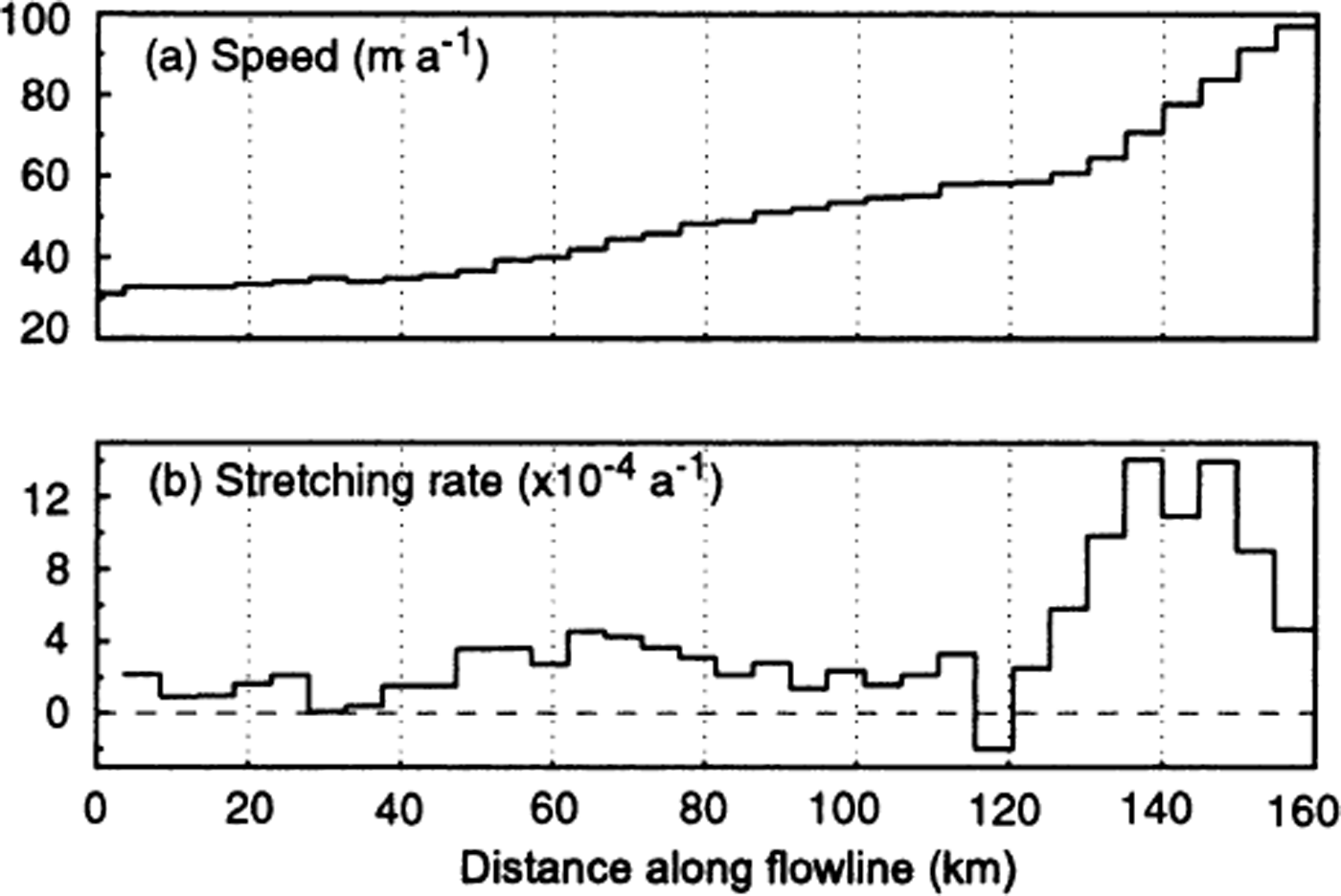
The production of meltwater upstream from, and the storage of basal water near to, the ice-stream onset are likely to be of central importance to the onset’s location. The largest site of possible subglacial ponding in the region, some tens of km upstream from the onset, is one at which important changes in the ice flow occur. Basal drag begins a steady decline shortly downstream from this location, and lateral drag begins a steady increase (Fig. 7d and c, respectively). Both are related to the dramatic increase in ice speed that occurs at this location, as indicated by an increase in the longitudinal stretching rate by a factor of ∼2–5 (Fig. 9a and b, respectively).

It is useful to examine the current study area in the context of Reference RaymondRaymond’s (2000) “stable” ice-stream states. In the meltwater “production-limited” state, basal sliding is fast but basal drag is small (e.g. Whillans Ice Stream). An increase in sliding speed does not increase the frictional melting rate, and so the basal meltwater system is buffered against the initiation of a positive feedback between frictional melting and basal sliding. In the “drainage-limited” state, basal sliding and basal drag are both large, so an increase in either quantity increases the frictional melting rate. Increased melting, however, is accommodated by the drainage or storage capacity of the basal water system. Again, the system is buffered against a positive feedback between basal melting and sliding. The stable, drainage-limited state could switch to an unstable state, however, in the event that meltwater generation exceeds the basal water system’s capacity for drainage or storage. Near to and upstream from the ISD onset, sliding speed, basal drag and frictional melting are large, as is the apparent capacity for basal water storage. These factors may promote a drainage-limited state, in which the basal water system is buffered against short-term increases. On the other hand, the system could switch to an unstable state in the event that the storage capacity was exceeded. A delicate balance between the stable and unstable states would exist in the event that the storage area became “full”. The basal water flux to downstream regions, including the onset, would then be highly sensitive to changes in the local surface slope and to any changes in the basal water flux from upstream.
Our observations and force-balance analysis suggest that the tributary regions upstream from the ice-stream onset may be as important to the initiation of ice-stream flow as are conditions at the onset itself. The tributaries are extended regions over which basal drag, basal sliding and basal lubrication become progressively more uniform along-flow. The integrated response, evident at the onset, is a weakened connection between the ice and bed and a shift from flow resistance at the bed to flow resistance at the margins. This characterization of the downstream initiation of an ice stream differs from some previous hypotheses, which attribute the onset of streaming flow to basal characteristics alone (e.g. Reference Anandakrishnan, Blankenship, Alley and StoffaAnandakrishnan and others, 1998; Reference BellBell and others, 1998). Here, the onset arises as a result of dynamic interaction between the ice flow and bed over the full length of the tributary upstream. An important implication of this is that temporal changes in flow along and upstream from the tributary may propagate downstream and affect the onset; changes upstream from an onset may result in changes at the onset. This characterization provides a physical basis for understanding current observations of non-steady behavior in other ice-stream onset regions (e.g. Reference Price and WhillansPrice and Whillans, 2001).
Conclusions
All terms in the force balance are important to ice flow in the ISD tributary and onset region. Driving stress is supported largely by basal drag, but with significant modifications by both non-local stress gradient terms. Near the ice-stream onset, basal drag decreases to ≤50% of the driving stress. Lateral drag supports an increasing fraction of the driving stress with distance downstream, up to ∼50–100% at the onset. The mean magnitude of longitudinal stress gradients in the study region is ∼20% of the mean driving stress, indicating that they too are significant to the balance of forces. Their effect is to decrease the variability in the basal drag imposed by large local fluctuations in the driving-stress field.
Frictional energy dissipation at the bed generates basal meltwater at a mean rate of ∼0.004 m a over the majority of the tributary. Locally, rates of basal melting may exceed 0.02 m a−1. The hydraulic potential gradient indicates that basal meltwater storage may coincide with areas of small basal drag. One site of possible water storage, ∼30 km upstream from the onset, extends across nearly the full width of the tributary. Basal drag decreases along-flow at this site, while ice speed, longitudinal stretching and lateral drag increase. Meltwater storage here may be crucial to the loss of mechanical control at the bed that becomes evident at the ice-stream onset.
Longitudinal stress gradients may be of particular importance to the flow transition that takes place along the ISD tributary. They result in a more spatially constant distribution of basal drag, frictional meltwater generation and basal sliding. The increased extent of basal lubrication and basal sliding provided by longitudinal coupling likely results in a weakened connection between the glacier and the bed, with the consequence that flow resistance switches from the bed to the margins. This switch is a key indication that the change from inland to streaming-style flow has been achieved.
The redistribution of energy dissipation at the bed provided by lateral stress gradients has been shown to be important in determining stable or non-stable states of basal lubrication (and thus sliding) at the bed of a mature ice stream (Reference RaymondRaymond, 2000). The current study indicates that longitudinal stress gradients may have similar importance to basal energy dissipation along upstream tributaries and near ice-stream onsets. Because sliding speed and basal drag are both relatively large in these regions, the possibility for feedbacks between frictional melting and basal sliding exists. The initiation of such a feedback would likely affect the spatial stability of the onset region over time.
Acknowledgements
The authors thank J. Fastook, T. Scambos and an anonymous reviewer for helpful comments. Informal discussions with C. Raymond stimulated overall improvement of this work. The SAR amplitude image used in Figure 1 is courtesy of The Byrd Polar Research Center (RADARSAT-1 Antarctic Mapping Project) at The Ohio State University. This work was supported by U.S. National Science Foundation grant OPP-9616394.
Appendix
Errors and Simplifying Assumptions
Uncertainties in the force-balance calculation derive from several sources: (1) measurement error; (2) the interpolation of data to a regularly spaced grid; (3) simplifying assumptions in the derivation of the force-balance equations.
Measurement uncertainties are the smallest source of error in the force-balance calculation. Table 1 shows 1σ uncertainty estimates for measured quantities and for the variables derived from them. Uncertainties in the measured velocities (0.12 m a−1) result in uncertainties in the calculated strain rates of ∼3.4 × 10⁻⁵ a−1. The signal-to-noise ratio for both velocity and strain rates is ≥100 (Reference Chen, Bindschadler and VornbergerChen and others, 1998). Uncertainties in the ice thickness are ∼50 m (assuming similar errors to those quoted in Reference Blankenship, Alley and BindschadlerBlankenship and others, 2001).
Two small error sources in the force-balance calculation arise from interpolation. First, shifting data from the survey grid to a regularly spaced calculation grid may introduce error. The offset between survey grid locations and the calculation grid is small, about 0.1 km, and errors here should be minor. Second, the finite-difference calculation method itself introduces uncertainty into the driving-stress field. Terms on the RHS of Equation (2) apply at gridcell corners, while surface slope (and hence the driving stress) calculated from field data applies to gridcell centers. To rectify this, surface elevations are interpolated to gridcell centers using a cubic convolution algorithm (other algorithms were tested with no significant difference in the resulting elevation field). Surface slope (and driving stress) at gridcell corners are in turn calculated from interpolated elevations at gridcell centers. While the uncertainties in the measured surface elevations are very small (∼0.015 m), surface elevations may vary considerably over the distance between gridcell corners and gridcell centers. We estimate the error due to the required interpolation by calculating the variance in surface elevation relative to a linear surface over the distance between cell corners and centers, using an airborne later altimetry dataset. The 90 km long, along-flow flight-line originates near the ISD onset, and the measurement interval is ∼9 m (unpublished data, collected for R. Bindschadler by The Support Office for Aerogeophysical Research). The standard deviation in elevation along this flight-line, computed for 2.5 km segments, is ∼1.5 m. We adopt this value as the uncertainty in surface elevation at gridcell centers (Table 1). While this uncertainty is large compared to the elevation measurement uncertainty, its contribution to the overall error budget is relatively minor; the uncertainty in the driving stress is generally ≤10 kPa.
The largest uncertainties in the force-balance calculations may be introduced through the simplifying assumptions in the derivation and application of Equations (2–7). We discuss the various assumptions and their estimated effect on the calculation results individually below.
In the strictest sense, Equation (2) is valid only if surface velocities apply throughout the full thickness of the glacier. For ice that is frozen to the bed and moving only by internal deformation, the ratio of depth-averaged velocity to surface velocity is ∼0.8. Basal sliding is a large fraction (∼2/3) of the measured velocity throughout the study area (Fig. 4b). This suggests that the ratio of depth-averaged to surface velocity is > 0.8 and that
![]() . Furthermore, the upper two-thirds of the ice column is cold and stiff relative to the lower third, and so serves as a “stress guide” (Reference Van der Veen and WhillansVan der Veen and Whillans, 1989b;Reference Whillans and van der VeenWhillans and Van der Veen, 1993). Surface strain rates are then representative of the stresses supported by the strong, uppermost “lid” of the glacier. Near Byrd Station, where velocities are small and the depth-independent velocity assumption would result in the largest magnitude errors, Reference Van der Veen and WhillansVan der Veen and Whillans (1989b) found little difference between force-balance calculations using the full-thickness approximation (used here) and calculations that took into account the depth variation in velocity and strain rate. Thus, we also assume that horizontal strain rates dominate the effective strain rate in Equation (7), allowing for the omission of vertical-shearing terms.
. Furthermore, the upper two-thirds of the ice column is cold and stiff relative to the lower third, and so serves as a “stress guide” (Reference Van der Veen and WhillansVan der Veen and Whillans, 1989b;Reference Whillans and van der VeenWhillans and Van der Veen, 1993). Surface strain rates are then representative of the stresses supported by the strong, uppermost “lid” of the glacier. Near Byrd Station, where velocities are small and the depth-independent velocity assumption would result in the largest magnitude errors, Reference Van der Veen and WhillansVan der Veen and Whillans (1989b) found little difference between force-balance calculations using the full-thickness approximation (used here) and calculations that took into account the depth variation in velocity and strain rate. Thus, we also assume that horizontal strain rates dominate the effective strain rate in Equation (7), allowing for the omission of vertical-shearing terms.
Converting deformation rates to stresses requires an estimate for the temperature-dependent rate factor, B (Equations (4) and (5)). Here, we use a rate factor based on a depth-averaged temperature from the profile measured in the Byrd Station borehole, located in the upstream, northern part of the study area (Fig. 1). Some uncertainty may be introduced into the force-balance calculation by assuming that this temperature profile, normalized by the ice thickness, applies over the entire study area. This uncertainty is likely largest for ice entering the study area from the south, from the BST. The thick ice in this region (∼3500 m) is likely warmer and softer at depth, relative to the ice entering the study area from near Byrd Station. Instead of trying to estimate a spatially variable rate factor, we assume that the uncertainty in the rate factor is large, about 1/3, or ∼170 kPa a1/3.
Strain-induced softening of the margins in the study region is likely to be insignificant, unlike the situation on the ice-stream trunks (e.g.Reference Whillans and van der VeenWhillans and Van der Veen, 1997). The largest shear-strain rates along the lateral margins of the ISD survey grid are an order of magnitude less than those along the margins of the mature ice-stream trunks (Reference Bindschadler, Vornberger, Blankenship, Scambos and JacobelBindschadler and others, 1996; Reference Whillans and van der VeenWhillans and Van der Veen, 1997). Thus, strain softening at the margins is not accounted for in the present calculation. We do note, however, that ice along the southern part of the study area may be relatively warm. Some fraction of the large shear-strain rates along this margin may then be due to softer, weaker ice there. In that case, the calculated lateral drag along the southern margin may be overestimated.
The driving stress used in Equation (2) derives from slopes differenced over 5 km, which is ∼2.5 times the mean ice thickness. This is slightly less than the (3–4) × H slope-averaging distance suggested in previous studies as necessary to avoid accounting for “bridging effects” (Reference Van der Veen and WhillansVan der Veen and Whillans, 1989a) or Budd’s (1970) “T” term. Bridging effects arise when a part of the bed supports relatively more or less than the local ice-overburden pressure. For ice flow near Byrd Station, Reference Van der Veen and WhillansVan der Veen and Whillans (1989b) found that including the bridging-effects term in the force-balance calculation altered the value of the calculated basal drag by ≤4 kPa. This is less than our estimate for the uncertainty in the driving stress, and ∼5% of the mean value for the calculated basal drag. It seems reasonable to conclude that omission of the bridging-effects term in the current study results in negligible errors.