Scholars, practitioners, and policymakers have all begun to recognize the importance of crime hot spots for doing something about the crime problem. However, this recognition of the potential for effective place-based interventions at crime hot spots has not led to broad investigation of the social structure and social context of these places. One reason for this is the dominance in the early interests of scholars of micro geographic hot spots in opportunities for crime and routine activities. Opportunity theories provided strong justification for investigating the micro geographic places where crimes occur. Indeed, such theories were tied to much of the early investigation of crime hot spots.

At the same time, scholars have for most part ignored the social structure and social context of crime hot spots, arguing that it is not important for untangling the relationship between crime and place (Braga and Clarke, Reference Braga and Clarke2014; also see Sherman et al., Reference Sherman, Gartin and Buerger1989). Our approach, as we explained in Chapter 1, is quite different from this. People who live on and visit a street segment get to know one another and become familiar with each other’s routines (Wicker, Reference Wicker, D. Stokols and I. Altman1987). Residents develop certain roles they play in the life of the street segment (e.g., the busybody and the organizer). Norms about acceptable behavior develop and are generally shared. Blocks have “standing patterns of behavior” (Barker Reference Barker1968, p. 18); for example, people whose routines are regular, like the mail carrier or the shop owner. Street segments in this context are perhaps the first building blocks of community. They are micro-communities, and in this sense, social structure and social context, not simply opportunities for crime, are important to examine (Sampson, Reference Sampson2003; Weisburd et al., Reference Weisburd, Groff and Yang2012).

In this chapter, we want to bring social structure and social context into the story of crime hot spots. We begin by examining why criminologists had for the most part ignored micro geographic study of crime until the late twentieth century. This was, in part, the result of not having data available at the micro geographic level, but also related to the overriding interests of sociologists concerned with meso-geographic units, such as neighborhoods and communities, in the study of spatial criminology. We then turn to the importance of new theoretical innovations that focused on hot spots of crime but led criminologists to mostly ignore the social structure and social context of these places. Having placed the study of crime hot spots in historical perspective, we bring social structure and social context into the study of crime and place by examining variability of measures of social disadvantage and social disorganization across hot spot and non–hot spot streets in our study. We pay particular attention to informal social control, which is generally measured in terms of what sociologists have called collective efficacy (Sampson et al., Reference Sampson, Raudenbush and Earls1997). We also examine characteristics of hot spots that are often seen as tightly linked to crime, such as social and physical disorder and fear of crime.

2.1 Ignoring the Micro geographic Environment

When criminologists first began to consider hot spots of crime in the late 1980s, they were confronted with a landscape that had little interest in micro geographic places as a unit of analysis. Most of criminology was focused on offenders and trying to understand why they became involved in crime (Weisburd, Reference Weisburd2015; Weisburd and Piquero, Reference Weisburd and Piquero2008). The distancing of criminology from micro geographic places came early and is well expressed by Edwin Sutherland (Reference Sutherland1947) in his groundbreaking textbook on criminology. Sutherland recognized the importance of place in the crime equation even as he presented his theory of differential social learning among individuals. He noted that “a thief may steal from a fruit stand when the owner is not in sight but refrain when the owner is in sight; a bank burglar may attack a bank which is poorly protected but refrain from attacking a bank protected by watchmen and burglar alarms” (Reference Sutherland1947, p. 5). Nonetheless, like other early criminologists (e.g., Hirschi, Reference Hirschi1969; Merton, Reference Merton1938; Sykes and Matza, Reference Sykes and Matza1957), Sutherland did not see such places as a relevant focus of criminological study. This was the case, in part, because crime opportunities provided by places were assumed to be so numerous as to make crime prevention strategies targeting specific places of little utility for theory or policy. In turn, criminologists traditionally assumed that situational factors played a relatively minor role in explaining crime as compared with the “driving force of criminal dispositions” (Clarke and Felson, Reference Clarke and Felson1993; Trasler, Reference Trasler, Clarke and Felson1993).

Similarly, early criminologists who did look at geography, gave little attention to the micro geographic environments in which crime occurred. These scholars generally had access to crime at the level of large administrative areas which allowed them to observe the spatial patterns of crime at a macro-geographic level, and to link demographic characteristics such as education or poverty with crime levels (e.g., see Guerry, Reference Guerry1833; Ducpétiaux, Reference Ducpétiaux1827; Quetelet, Reference Quetelet1831). Such data was beginning to be collected routinely by European governments, and provided an opportunity for cartographers, statisticians, and geographers to examine the crime problem in new and insightful ways (e.g., see also Glyde, Reference Glyde1856; Quetlet, Reference Quetelet1842).

The nineteenth century criminologists in Europe did not examine micro geographic trends in good part because such data were unavailable. The management information systems that now provide police data at the addresses where crimes occur were not to come into existence until the second half of the twentieth century (Weisburd and McEwen, Reference Weisburd, McEwen, Weisburd and McEwen1997). Regardless, the study of crime at the macro-geographic level in the nineteenth century was a major advance in studying spatial criminology, but the governmental data sources available did not bring crime down to the micro geographic level.

At the same time, a few nineteenth-century European criminologists began to challenge drawing strong conclusions about crime when looking at macro-geographies. John Glyde (Reference Glyde1856) from England, for example, questioned the validity of research findings when large areas were chosen as units of analysis in geographic criminology. In his paper “Localities of crime in Suffolk,” he showed very clearly that larger units of analysis hide underlying variations in crime. When considering units smaller than districts, significant differences in crime rates across smaller areas appeared. Similarly, Henry Mayhew (Reference Mayhew and Quennell1851) tried to uncover patterns in the distribution of crime in the city of London by combining ethnographic methods with statistical data. He interviewed prostitutes, criminals, and other citizens about alcoholism, poverty, housing conditions, and economic uncertainty. He was the first scholar who focused on small areas such as squares, streets, and buildings as units of analysis in criminological research, predating modern interests in the criminology of place by over a century. European criminologists, however, did not follow up on these insights, likely because such data were so difficult to collect.

After the turn of the twentieth century, the locus of geographic research on crime moved to the United States (Beirne and Messerschmidt, Reference Beirne and Messersmidt1991; Bulmer, Reference Bulmer1984; Faris, Reference Faris1967; Harvey, Reference Harvey1987). University of Chicago sociologists such as Robert Park, William Thomas, Louis Wirth, Ernest Burgess, Clifford Shaw, and Henry McKay took a leadership role in advancing a theory of social disorganization that focused on neighborhoods or communities. The unit of analysis of geography was generally defined in smaller units than the administrative areas of European criminology in the nineteenth century, but was still much removed from the micro geographic studies of crime and place that have recently focused criminologists’ attention on hot spots of crime. The concern of this new school of criminology can be seen as focusing on meso-geographic areas, which they defined as neighborhoods. A distinct problem of this approach was that administrative data available in Chicago, where most empirical studies were carried out, were generally not defined in this way, which made the development of research in this tradition very difficult. It was not until the 1970s that the census provided detailed social information at the level of census block groups, which have become an important source for study of crime by community criminologists, such as the Project on Human Development in Chicago Neighborhoods (PHDCN) (e.g., Sampson, Reference Sampson2012; Sampson et al., Reference Sampson, Raudenbush and Earls1997).

2.2 Social Disorganization and Crime in Communities

The theoretical idea that lay behind the study of communities and crime by the Chicago School of criminologists was introduced by William Thomas, who noted that the concept of social disorganization, could be defined as “a decrease of the influence of existing social rules of behavior upon individual members of the group” (see Thomas and Znaiecki, Reference Thomas and Znaniecki1918, p. 1128). Robert Park, who was recruited by Thomas, was the initiator of urban social research on communities and crime, shifting the unit of analyses from countries and large areas to cities and their neighborhoods (Park, Reference Park and Burgess1925 [1967]). The city, in his opinion was more than:

Park argued that urban life must be studied in this context in terms of “its physical organization, its occupations, and its culture” and especially the changes therein (Park, Reference Park and Burgess1925 [1967], p. 3). Neighborhoods in his view were the elementary form of cohesion in urban life.

His younger colleague, Ernest Burgess, drawing from an inventory of price changes in housing values in Chicago areas, developed a concentric zone model of the distribution of social problems and crime for cities (especially for Chicago) (Burgess, Reference Burgess, Park and Burgess1925 [1967]).Footnote ¹ Burgess suggested that Chicago included five concentricFootnote ² zones, each containing various neighborhoods, four of them situated around ‘The Loop’ (the business center of the city): “the typical processes of the expansion of the city can best be illustrated, perhaps, by a series of concentric circles, which may be numbered to designate both the successive zones of urban extension and the types of areas differentiated in the process of expansion” (Burgess, Reference Burgess, Park and Burgess1925 [1967], p. 50). Burgess’ unit of analyses was a series of neighborhoods within cities that share similar characteristics. He assumed that depending on the distances to the center and the structural features of these zones, the levels of crime would vary.

Clifford Shaw was one of the first Chicago sociologists to carry out extensive empirical research on the geographical distribution of crime based on Burgess’ zone model (Shaw, Reference Shaw1929). In 1942, Shaw and Henry McKay published their magnum opus Juvenile Delinquency and Urban Areas in which they not only presented their geographical and etiological analyses of crime rates in the city of Chicago, but also those of other cities: Philadelphia, Boston, Cincinnati, Cleveland, and Richmond (Shaw and McKay, 1942 [Reference Shaw and McKay1969]). In all the cities studied, they found similar patterns in the geographical distribution of crime. However, the units of analysis differed a good deal between the various cities. These differences were due to the lack of detailed official crime data in cities other than Chicago. The rapid changes in the city of Chicago over a long period of time enabled them to also study the effects of the city dynamics on crime and other phenomena. One of their findings was that “(t)he data on trends also demonstrate with equal sharpness the rapid rise in rates of delinquents in certain areas when a population with a different history and different institutions and values takes over areas in a very short period of time” (Shaw and McKay, 1942 [Reference Shaw and McKay1969], p. 382). They identified “delinquency areas” and identified structural features of these areas that were related to crime, such as high infant mortality, overpopulation, poverty, and high rates of mobility.

While the Chicago School researchers focused on neighborhoods, Shaw (Reference Shaw1929) began his efforts to identify delinquency areas with a micro geographic focus on data collection. He did not begin with data on large areas, but with plotting the home addresses of thousands of juvenile and adult offenders on a map of Chicago:

Shaw’s confident assertion that the “study of such a problem as juvenile delinquency necessarily begins with a study of its geographical location” was not heeded by those who followed him (Shaw, Reference Shaw1929, p. 10). We suspect that the difficulty of creating these micro geographic maps of crime discouraged other researchers from studying crime at a micro geographic level. But more generally, the theoretical focus of the Chicago School was not on micro geographies but rather on meso-geographic units such as neighborhoods or in Shaw and McKay’s (1942 [Reference Shaw and McKay1969]) case, on delinquency areas.

Structural features of neighborhoods or communities were the primary interests of these pioneering criminologists, which they saw as reflecting the degree to which informal social controls could be marshalled to prevent crime (Burgess, Reference Burgess, Park and Burgess1925 [1967]; Park and Burgess, Reference Burgess, Park and Burgess1925 [1967]; Shaw, Reference Shaw1929; Shaw and McKay, 1942 [Reference Shaw and McKay1969]). Such failures of social organization were seen to be the result of the heterogeneity of populations, residential turnover, and poverty, and related social disorganization found in specific urban neighborhoods in the city (Bellair, Reference Bellair1997; Hipp, Reference Hipp2007; Mazerolle et al., Reference Mazerolle, Wickes and McBroom2010; Sampson and Groves, Reference Sampson and Groves1989; Shaw and McKay, 1942 [Reference Shaw and McKay1969]; Silver and Miller, Reference Silver and Miller2004; Warner and Pierce, Reference Warner and Pierce1993; Warner and Rountree, Reference Warner and Rountree1997). In such areas, social ties are weak, and residents do not invest in relationships necessary for informal social control, such as supervising youth, and self-regulation through shared values, resulting in the presence of high crime rates (Kasarda and Janowitz, Reference Kasarda and Janowitz1974; Kornhauser, Reference Kornhauser1978; Bursik and Grasmick, Reference Bursik and Grasmick1993).

2.3 Bringing Hot Spots of Crime into the Crime Equation

When criminologists began to observe the concentration of crime at crime hot spots in the 1980s and 1990s (Pierce et al., Reference Pierce, Spaar and Briggs1988; Sherman and Weisburd, Reference Sherman and Weisburd1995; Sherman et al., Reference Sherman, Gartin and Buerger1989; Spelman, Reference Spelman, Eck and Weisburd1995; Weisburd and Green, Reference Weisburd and Green1995; Weisburd et al., Reference Weisburd, Maher, Sherman, Adler and Laufer1992), they found little in criminological thinking that would suggest the importance of micro geographic places in the production or prevention of crime. As we noted earlier, much of traditional criminology was focused on understanding why individuals commit crime. In turn, when criminologists in the last century were concerned with places, they focused on meso-geographic areas such as delinquency areas or communities.

In this context, criminologists who began to study hot spots of crime in the 1980s and 1990s, saw little relevance of social disorganization, which had been linked strongly to communities and neighborhoods, to micro geographic places. Sherman et al. (Reference Sherman, Gartin and Buerger1989) who first introduced the idea of a criminology of place noted: “Traditional collectivity theories [such as social disorganization theory] may be appropriate for explaining community-level variation, but they seem inappropriate for small, publicly visible places with highly transient populations” (p. 30). More recently, Braga and Clarke (Reference Braga and Clarke2014) argued that the application of social disorganization to micro geographic hot spots goes beyond the original domain of these theories (see also Schnell et al., Reference Schnell, Braga and Piza2017). Such theories are large area-level theories, and they doubt that such community level theories “can adequately explain why a particular crime spot is persistently hot over time” (Braga and Clarke, Reference Braga and Clarke2014, p. 488).

Opportunity theories, which started to gain notice in criminology in the 1970s, appeared much more relevant to the new interest in hot spots of crime since they explicitly recognized the key role that micro geographic places play in the production of crime. For example, in 1979, Lawrence Cohen and Marcus Felson, were to suggest a new way to think about the crime problem that departed radically from traditional criminology and placed micro geographic places in the center of the crime equation. They argued that a more complete understanding of crime must include a recognition that the availability of motivated offenders, suitable crime targets, and the presence or absence of capable guardians all influence crime events (Cohen and Felson, Reference Cohen and Felson1979). Importantly, these three components of a crime event must converge in time and space for a crime to occur. The “space” that Cohen and Felson were referring to was the specific micro geographic places where crimes take place. In their theory of routine activities and crime, a crime could only occur if motivated offenders and suitable targets come together at a specific place where there is the absence of capable guardianship:

The importance of micro geographic places was also to be key to the development of “situational crime prevention” (Clarke, Reference Clarke1983). Situational crime prevention moved the critical unit of analysis of crime away from the people who commit crime to the situations in which crime occurs. Situational crime prevention is concerned with the “opportunity structures” of specific contexts and places. By opportunity structure, advocates of this perspective are not referring to the broad societal structure of opportunities that underlie individual motivations for crime (e.g., see Merton, Reference Merton1938), but to the immediate situational components of the context of crime. Importantly, place at a “micro” level is key to situational crime prevention theory since it focuses on the immediate opportunities for crime, which are generally structured within very small geographic areas.

Around the same time as routine activities theory and situational crime prevention developed, Paul and Patricia Brantingham published their seminal book Patterns in Crime, which emphasized the role of place characteristics and human activity in shaping the type and frequency of human interaction (Brantingham and Brantingham, Reference Brantingham and Brantingham1984). Crime pattern theory explores the distribution and interaction of targets, offenders, and opportunities across time and space (Brantingham and Brantingham, Reference Brantingham and Brantingham1981). The importance of micro geographic places is essential to crime pattern theory. Not only are places logically required (an offender must be in a place when an offense is committed), but also the characteristics of places are seen to influence the likelihood of crime and the likelihood that specific places will become crime hot spots.

These theoretical innovations in the twentieth century provided a logic for why micro geographic places are important to understanding and preventing crime, and they naturally informed study of crime hot spots. However, we think that the predominance of these theoretical perspectives has led to a myopia in which the social structure and social context of crime hot spots has been ignored. Our work seeks to bring social structure and social context into the study of crime hot spots, because we begin with the assumption that such hot spots are not only physical environments but also social environments. They are also social settings or, following Wicker (Reference Wicker, D. Stokols and I. Altman1987, p. 614), “behaviour settings” that can be seen as “small-scale social systems” or small-scale communities (Sampson, Reference Sampson2003; Taylor, Reference Taylor1997; see also St. Jean, Reference St. Jean2007). They have many of the traits of communities that have been seen as crucial to social disorganization theory in that these physical units also function as social units with specific norms and routines. In turn, if micro geographic units such as street segments can be seen as a type of “micro-community” (Sampson, Reference Sampson2003; Weisburd et al., Reference Weisburd, Groff and Yang2012), then social structure and social context should have direct relevance to our understanding of the level of crime on street segments.

2.4 Social Disorganization and Social Structure at Street Segments

In trying to understand how social disorganization develops in communities, criminologists have focused on a series of indicators that suggest structural factors that can impede the development of social organization or informal social control. Some of these are traditional demographic measures, for example, poverty or low educational achievement (Sampson, Reference Sampson2012; Shaw and McKay, 1942 [Reference Shaw and McKay1969]). Such disadvantages are accented by racial discrimination and disparities. Together these characteristics of communities lead to what sociologists have called concentrated disadvantage (Sampson, Reference Sampson2012; Sampson et al., Reference Sampson, Morenoff and Gannon-Rowley2002), which inhibits the ability of residents to carry out collective action and subsequently leads to low community social control (Sampson et al., Reference Sampson, Raudenbush and Earls1997). There is strong evidence of the relationship between concentrated disadvantage and crime in communities (Armstrong et al., Reference Armstrong, Katz and Schnebly2015; Gerell and Kronkvist, Reference Gerell and Kronkvist2016; Mazerolle et al., Reference Mazerolle, Wickes and McBroom2010; Morenoff et al., Reference Morenoff, Sampson and Raudenbush2001; Sampson et al., Reference Sampson, Raudenbush and Earls1997; Zahnow et al., Reference Zahnow, Corcoran, Kimpton and Wickes2022). Do we similarly find a strong relationship between hot spots of crime and concentrated disadvantage in our study?

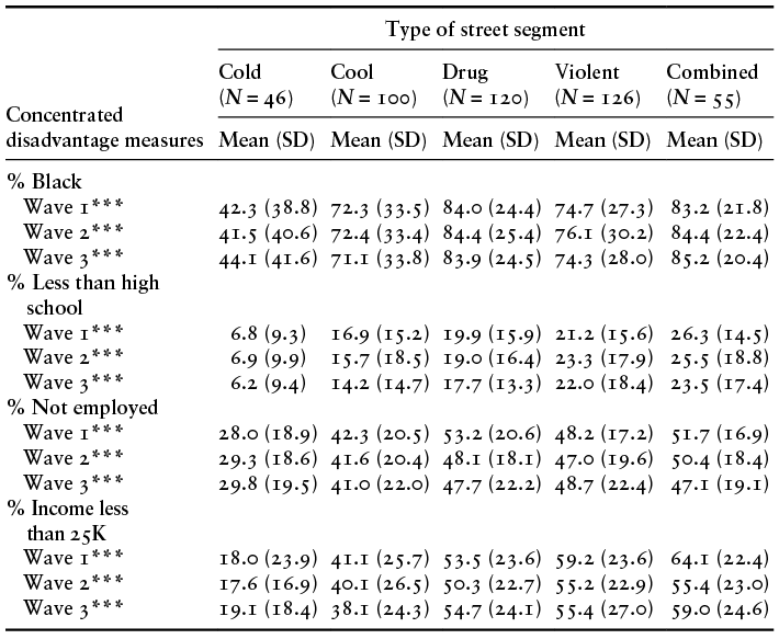
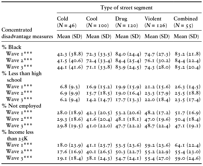
In Table 2.1, we present four indicators of social and structural disadvantage measured across the five street types we described in Chapter 1 – percent Black, percent with less than a high school diploma, percent not employed, and percent earning less than $25,000 annually. Importantly, when possible in this chapter, we provide results for each of the three waves of our study.Footnote ³ This allows us to identify the degree of stability of outcomes across the waves of data collection. In turn, samples are in the end, samples, and not populations, and our collection of multiple waves of data provides an ability to guard against drawing strong conclusions from unusual outcomes that might reflect sampling outcomes in a specific wave of data.

Table 2.1Demographics capturing concentrated disadvantage by segment type

Note:

^*** p < 0.001 from ANOVAs.

We find significant differences across street types for racial composition of the streets across three waves (Table 2.1). We also find that the samples across all three waves are very consistent. The differences observed are most apparent in comparing streets with little crime, what we term “cold spots,” with other streets in the sample. While about 40% of the samples of cold spot streets are Black, this is true for more than 70% of the other street types. It should be remembered that 64% of residents of Baltimore were defined as Black during the period of our study (US Census Bureau, 2015). Overall, hot spots of crime have higher rates than this, but so does our sample of “cool spots.” It is important to note that cool spots in our sample evidence some degree of crime, but fail to reach the 3 percent threshold for violent and drug crime that we set in our sampling approach.

Looking at the percent of residents with less than a high school education, we again find statistically significant differences, with cold streets being very different from hot spot streets. While less than 7% of the residents of cold spot streets have less than a high school education, this is true for between 17.7 and 26.3% across the three hot spot types and three waves of data collection. The cool spot streets fall somewhere in between.

Approximately half of the residents of hot spots streets are not employed, and these outcomes are consistent across the three waves. This is true for less than 30% of residents of cold spot streets, and about 40% of residents of cool spot streets. Again, the differences between the street types are statistically significant, as are differences in yearly income. Over 50% of the residents of the hot spot streets across the three waves had household incomes below $25,000. Alternatively, fewer than 19.1% of residents of cold spots and about 40% of households of cool spot streets earned less than $25,000 a year.

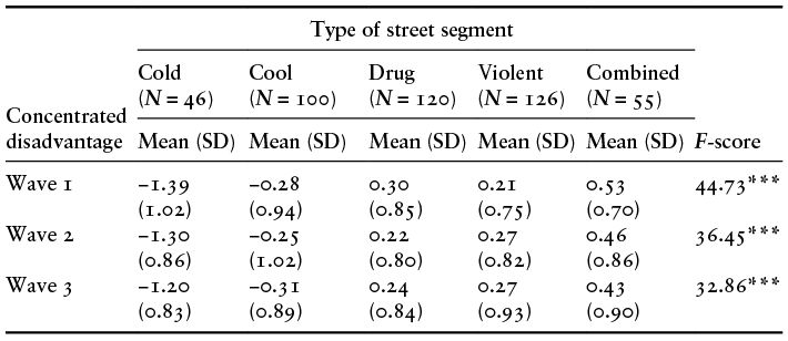
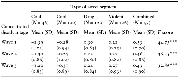
Examining a measure that combines these indicators into a single scale of concentrated disadvantage reinforces the idea that social/structural disadvantage is much greater at hot spots of crime (see Table 2.2).Footnote ⁴ The differences between the streets are statistically significant, with the largest contrasts being between the cold spot streets and the combined violent and drug crime streets. At the same time, we can see strong differences between the hot spot streets and both the cold and cool spot streets. Both cold and cool spot streets have negative values on our scale, while all of the hot spot street types have positive values.

Table 2.2Concentrated disadvantage factor score by segment type

Note:

^*** p < 0.001; Overall mean for waves 1, 2, and 3 is 0.

Residential tenure and home ownership are two other key social structural measures of communities which are seen to “promote collective efforts to maintain social control” (Sampson et al., Reference Sampson, Raudenbush and Earls1997, p. 919). The movement of populations in and out of communities was a key feature of early theories of social disorganization (Sampson Reference Sampson2012; also see Shaw and McKay, 1942 [Reference Shaw and McKay1969]), reflecting the breakdown of social controls when residents become isolated and unfamiliar with each other. Residential tenure and home ownership reflect stability of populations in many studies (Sampson Reference Sampson2012; Sampson et al., Reference Sampson, Raudenbush and Earls1997).

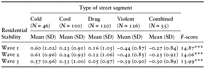
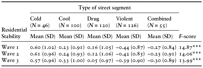
We created a factor score for residential stability, which combined measures of residential tenure and home ownership.Footnote ⁵ Overall, we find statistically significant differences between the streets across the three waves of data collection (see Table 2.3). And as in our earlier analyses, the cold spot streets have much higher levels of residential stability than combined hot spots. In this case, it appears that violence has a particularly important relationship to residential instability, as drug hot spots are closer in scores to cool spots than to the violent crime and combined violent and drug crime hot spots.

Table 2.3Residential stability factor score by segment type

Note:

^* p < 0.001; Overall mean for waves 1, 2, and 3 is 0.

2.5 Social Ties and Social Networks

Social ties and social networks have also been linked to social disorganization and community social controls (e.g., see Bellair, Reference Bellair1997; Bursik and Grasmick, Reference Bursik and Grasmick1993; Warner and Rountree, Reference Warner and Rountree1997; Wickes et al., Reference Wickes, Hipp, Sargeant and Mazerolle2017). It is assumed that when social ties and social networks are stronger, communities will be able to more effectively marshal informal social control (Hipp, Reference Hipp2022; Wickes and Lanfear, Reference Wickes, Lanfear, Oberwittler and Wickes2025; Sampson, Reference Sampson, Cullen, Wright and Blevins2006, Reference Sampson2012).

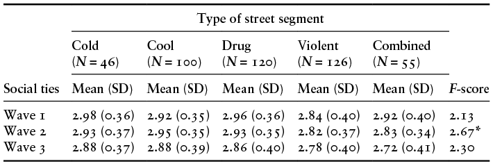
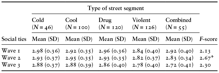
We measured social ties based on three questions from the survey that asked how often residents (1) “chat with neighbors,” (2) “visit with neighbors,” and (3) “help each other out.” Response options included “never (1),” “rarely (2),” “sometimes (3),” and “often (4).”Footnote ⁶ In this case, we find relatively smaller differences between the residents of the different types of streets (see Table 2.4). The differences here are not meaningful and are not statistically significant in the first and third waves of the study. Even in the second wave the differences between the streets are not large, and do not follow a clear pattern.

Table 2.4Social ties by segment type

Note:

^* p < 0.05; Overall mean for wave 1 = 2.91, overall mean for wave 2 = 2.89, and overall mean for wave = 2.83.

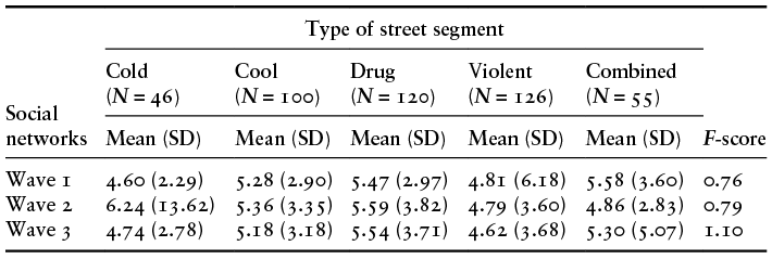
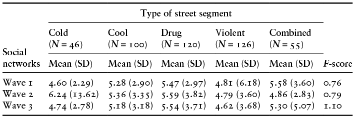
When it comes to the size of residents’ social networks – measured by asking residents how many of their neighbors on the street they consider to be friends – we again find similar results across hot spots, cool spots, and cold spots. Across all three waves, there were no significant differences in resident’s number of neighborly friends between the different types of streets (see Table 2.5).

Table 2.5Social networks by segment type

Note: Overall mean for wave 1 = 5.16, overall mean for wave 2 = 5.29, and overall mean for wave = 5.09.

These results may seem surprising at first glance. But our qualitative data provide a view of crime hot spots that in many ways is contradictory to the stereotypes held by laypeople and scholars alike. Our review of social structural features of hot spot streets shows that they are generally disadvantaged, especially as contrasted with streets with little or no crime. At the same time, it would be wrong to suggest that these streets are places where people have few ties to their neighbors. In our qualitative research, we heard numerous accounts of residents knowing their neighbors and spending time with them. A male in his fifties, who lived on a violent street for over twenty years, talked positively of the relationships between neighbors, even with changes in the area. He said, “I’ve known my neighbors for years and have no issues with them.” At the same time, he also acknowledged how people’s interactions have changed over time – “in the past we would be gathering outside our homes, sing, and play music etc., but now we tend to make those gathering inside our houses … people are less open than before – they shy out easily and prefer to stay behind the walls.”

Sometimes our qualitative field researchers would talk to someone who worked on the street or was visiting family on the street. One woman who regularly visited her sister, who lived on a violent street segment, mentioned that she “felt comfortable that her kids and family lived on that street,” and she “didn’t mind coming to visit … people are friendly enough, me and my family know a good amount of the neighbors and people get along all right.”

Just as residents of hot spot streets had stronger social ties than might have been assumed by levels of crime and structural disadvantage, it was not always the case that residents of non–hot spots had strong ties with their neighbors. We heard a few stories from residents who lived on cold and cool streets and indicated that while neighbors may know one another, people also kept to themselves. For example, a young female who lived on a cold street said that “the neighborhood mostly got along and it was quiet …. people don’t really do anything together but keep to themselves … people don’t really come out of their house to hang out or talk to one another.”

At the outset we want to distinguish between informal social control and nongovernmental efforts to reduce crime based on opportunity reduction approaches. John Eck and his colleagues have long argued that private guardianship (e.g., place managers) is an essential way in which crime can be reduced (Eck and Madensen-Herold, Reference Eck, Madensen-Herold, Nagin, Cullen and Jonson2018; Linning and Eck, Reference Linning and Eck2021). We saw evidence of such approaches in our qualitative data, where specific business owners or treatment facilities, located on crime hot spots, increased security measures. For example, a drug rehabilitation clinic was located on one of the drug hot spots and we spoke with the security officer – he noted his role in keeping “order” on the street and that “nuisance crimes are what escalate and when unchecked lead up to more violent crime and drug crime in the city.” On another violent hot spot, a business owner talked about how his “business hires private security to provide protection, they share the cost with a couple of other stores too.” Of course, there is a direct relationship between informal social control and such efforts. When levels of informal social control on a street are higher, people who live there are more likely to encourage and evidence guardianship whether by neighbors or more formal agents such as doormen or women, or other proprietary agents who control properties on the street, such as landlords.

2.6 Informal Social Control and Collective Efficacy

Despite the key importance of informal social control to social disorganization theory, most scholars until the late 1990s measured informal or community social control in relationship only to the social structural indicators we examined earlier (Bursik and Grasmick, Reference Bursik and Grasmick1993; Shaw and McKay, 1942 [Reference Shaw and McKay1969]). But by the 1970s, theorists began to emphasize the importance of directly assessing social control in the community. Kornhauser (Reference Kornhauser1978) made the case that social disorganization leads to crime because residents are unable to realize common values or solve shared problems within the community. Bursik and Grasmick (Reference Bursik and Grasmick1993) noted that informal social control is “the effort of the community to regulate itself and the behavior of residents and visitors to the neighborhood” (p. 15).

Sampson et al. (Reference Sampson, Raudenbush and Earls1997) proposed a direct measure of informal social control for communities. This measure extended the concept of social control to emphasize the capacity of a community to realize common values and regulate behavior through cohesive relationships and mutual trust among residents (see also Sampson, Reference Sampson, Cullen, Wright and Blevins2006, Reference Sampson2012). They termed this measure “collective efficacy” which was conceptualized as the willingness of neighborhood residents to take action and intervene, which relied on mutual trust among residents (Sampson et al., Reference Sampson, Raudenbush and Earls1997, Reference Sampson, Morenoff and Gannon-Rowley2002; Kubrin and Weitzer, Reference Kubrin and Weitzer2003). Collective efficacy measured informal community social control by combining two scales, one of willingness to intervene (also termed “shared expectations for informal social control”) and the other of social cohesion and trust. We follow Sampson et al.’s (Reference Sampson, Raudenbush and Earls1997) approach in assessing levels of informal social control on street segments (also see Sampson, Reference Sampson2012).Footnote ⁷

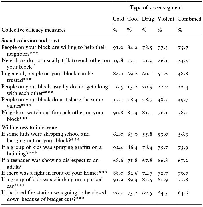
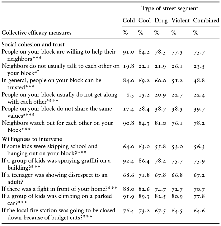
Before examining the overall scale results, we think it important to examine the specific items of the scale and their relationship to the street types in our study. Table 2.6 provides the average responses for wave 1 data for the distinct items in the two scales that make up the collective efficacy measure. The relationships observed are similar for waves 2 and 3.

Table 2.6Individual measures of collective efficacy by segment type (wave 1)

Note:

^* p < 0.05, ^***p < 0.001; % = Participants who responded “agree” or “strongly agree;”

Ns are at the individual level and vary between 3,727 and 3,737 for the individual items; ^a = item was reversed coded for creating the mean scale.

Looking at social cohesion and trust, we see that each item is statistically significant. As in earlier analyses, the largest differences are found between the combined violent and drug spots and the cold spots. The largest difference found is perhaps the most direct measure of trust: “in general people on your block can be trusted.” Here 84 percent of respondents on cold streets agreed or strongly agreed that people on their block could be trusted. In contrast, only 49 percent of respondents on combined streets agreed. On other social cohesion items, there are also large differences. For example, about 40 percent of residents of hot spots say people on their street do not share the same values, but this was true for only 17 percent of residents on cold spots. For this measure, violent crime hot spots are very similar to the combined violent and drug crime hot spots. Residents of drug hot spots report more positive levels on each of the social cohesion measures as compared with the other hot spots, and cool spot residents generally report more positive levels than drug hot spot residents.

While hot spots have much lower levels of social cohesion and trust, we think it would be a mistake to assume that levels of social cohesion at hot spots are negligible. Hot spots have significantly lower levels of social cohesion as measured by these individual items; yet we see here that social cohesion is far from absent on these streets. Even on the combined hot spot streets, more than three-quarters of residents say they are willing to help their neighbors. We think these findings emphasize that such streets are not places without social cohesion and trust, but rather where social cohesion and trust are less evident than on streets with little or no crime.

Measures of willingness to intervene show a similar set of relationships. The combined hot spots and violent crime hot spots have the lowest levels of willingness to intervene, and the cold spots have the highest levels. Drug hot spots and cool spots fall in between, with the drug hot spots evidencing generally less willingness to intervene. The differences are significant across the street types in every case, except for the measure of intervening in the case where a “teenager was showing disrespect to an adult.” Here about 70 percent of respondents on all streets answered agree or strongly agree. Again, it is important to note that the levels of willingness to agree are relatively high even for the combined drug and violent crime hot spots. More than six out of ten residents agree or strongly agree with almost every item.

These findings are also reflected in our qualitative interviews. For example, a woman who lived on a violent hot spot discussed how “there are drugs and crime nearby, but the street is quiet. At one point people tried to bring drugs and crime into the housing, but the neighbors got together to make sure that didn’t happen and pushed them out.” She continued, “the area is friendly, and people take care of each other, watch out for each other and each other’s kids.” On a drug spot, where a female in her twenties described concerns about safety for her children on the street, she still emphasized that “the neighbors generally look out for each other, and we are a close and a strong community.” She said, “a lot of people have lived in the area a long time and I feel like people are looking out for me.” She also highlighted that “people take care of each other more because they know what it’s like to be hungry and to struggle so they want to do what they can to keep someone else from having to go through that … people help each other because they know what it’s like.”

A resident of a drug hot spot said that the neighbors were friendly, and he and “a woman down the street got together and organized neighborhood meetings, and then coordinated residents to do trash pick up to make sure the neighborhood stayed clean and they didn’t have rats or other problems due to trash in the street.” He said, “people were good about following up on it and picked up the trash when they were supposed to.” When asked whether he would do more organizing in the community, he said “yes, but we’re just focused on the trash pick-up for now.”

One element of informal social control on the hot spot streets was the involvement of religious communities. Multiple streets where the qualitative data was collected had residents describe the role of the Muslim community on the street. On a violent hot spot, one resident noted that the Muslim community members “look out for each other and all of the kids in the neighborhood, and they keep the park near their mosque clean and the place around their community safe. They pick up trash and have their kids playing around on the playground, and it is better when people are outside.”

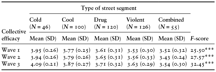
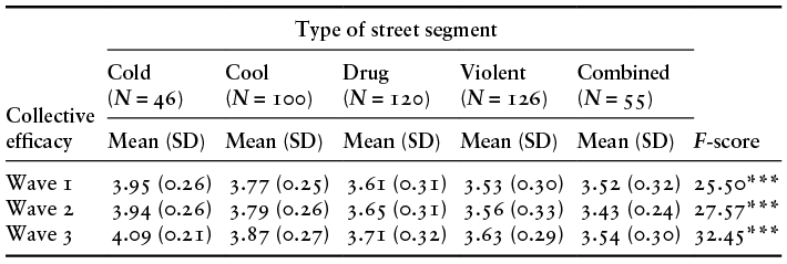
Even though both social cohesion and willingness to intervene are at higher levels than we might have expected absent empirical data on hot spot streets, we still find strong and significant differences in overall collective efficacy across the street types we examine (see Table 2.7).

Table 2.7Collective efficacy mean scores by segment type

Note:

^*** p < 0.001; Overall mean for wave 1 = 3.65, overall mean for wave 2 = 3.66, and overall mean for wave = 3.74.

In each wave we observe a consistent relationship between street type and collective efficacy. The combined violent and drug crime streets evidence the lowest levels of collective efficacy, followed by the violent crime hot spots, then the drug crime hot spot. Cool spots have higher collective efficacy than hot spots, and cold spots have the highest levels overall. This follows what social disorganization theorists predict, though we will more carefully examine the relationship between collective efficacy and crime using multiple waves of survey data while controlling for potentially confounding influences in Chapter 4.

The relationships we observe here are very consistent with the social structural variables we identified earlier in the chapter, but not similar to the measures of social ties and social networks, where we found little difference between hot spots and cool and cold spots. Shouldn’t social ties and social networks enable informal social controls? Robert Sampson and colleagues suggested one explanation for this incongruity in our data. They argue that social structural features of communities may inhibit the ability of residents to exercise informal social control. In this context, concentrated disadvantage can be seen as operating as a “centrifugal force that stymies collective efficacy” (Sampson et al., Reference Sampson, Raudenbush and Earls1997, p. 919; see also Gerstner et al., Reference Gerstner, Wickes and Oberwittler2019). They note that “even if personal ties are strong in areas of concentrated disadvantage, they may be weakly tethered to collective actions” (Sampson et al., Reference Sampson, Raudenbush and Earls1997, p. 919; Wickes and Lanfear, Reference Wickes, Lanfear, Oberwittler and Wickes2025).

2.7 “It Is Not as Bad as People Think It Is”: Rethinking Our Preconceptions about Hot Spot Streets

Our findings regarding social structure and social context on hot spot streets confirm the importance of our efforts to bring social disorganization and collective efficacy into the interests of the criminology of place. Hot spots of crime, as contrasted with non–hot spots, are places with high levels of concentrated disadvantage and relatively low levels of informal social control. In this sense our findings reinforce those of community-level studies that emphasize the importance of social disorganization in understanding crime, though we find this at the level of crime hot spots. At the same time, we think that our findings bring an important correction to the images of high-crime streets in academic and popular literature that we noted in Chapter 1. Despite starkly higher levels of crime, as described in Chapter 1, residents of hot spot streets have similar levels of social ties and social networks as residents of non–hot spot streets. Residents of hot spot streets also evidence lower levels of informal social control than streets with little crime, but just because there is not as much informal social control does not mean that there is none. These are not places of chaos and hopelessness; they possess meaningful levels of informal social control and guardianship (Weisburd, Uding, et al., Reference Uding, Porter, Dong and Moon2024; see also Weisburd, Kuen, et al., Reference Kuen, Appleton, Weisburd and Uding2025).

Many residents of hot spot streets are optimistic about the possibilities for their communities in the future. One resident told us that he was aware of the perception that most people had about neighborhoods like his but that “it’s not as bad as people think the place is.” It is not that residents of high-crime streets do not recognize the problems on their street; the point is that despite these problems, residents cared for their community and held out hope that things could get better. For example, one resident of a violent segment talked openly about weekly occurrences of violence and murders nearby but said that he “still loves [the street], – with concerns.” He talked about the sense of neighborhood and cooperation among the homeowners and about how he is coordinating a community organization to try to do the work that the city is not doing, such as cleaning and community policing. He was carrying papers on which he had written his observations about the area that he planned to discuss with neighbors next month, at their first meeting. He said, “I don’t know how successful the effort will be, but I’m crossing my fingers.”

2.8 Social and Physical Disorder and Fear of Crime

In Chapter 1, we described the crime levels of the streets, and how these were used to distinguish between the five street types. Before concluding our descriptive review of the social structure and social context of hot spot streets, we want to consider features of the streets often related to crime by scholars. Broken Windows theory, for example, links disorder and crime in a development sequence in which the inability of a community to control disorder leads to more serious crimes (Wilson and Kelling, Reference Wilson and Kelling1982). Sampson (Reference Sampson2012) and Sampson and Raudenbush (Reference Sampson and Raudenbush1999) have argued that social disorder is strongly related to crime (while highlighting that both are related to low levels of collective efficacy), and for that reason the two can often be conflated (see also Gau and Pratt, Reference Gau and Pratt2008). Given the importance of disorder in discussions of crime, we review measures of disorder below. We would expect a strong relationship between disorder and our street segment types given prior research in this area (Lane et al., Reference Lane, Rader, Henson, Fisher and May2014; Yang, Reference Yang2010). One consequence of crime and disorder is fear of crime (Brunton-Smith and Sturgis, Reference Brunton‐Smith and Sturgis2011; Kuen et al., Reference Kuen, Weisburd, White and Hinkle2022; Zhao et al., Reference Zhao, Lawton and Longmire2015). Again, scholars have generally seen fear as a consequence of crime and disorder, though there are many studies that show that this relationship is not necessarily objective and is often conditioned on the backgrounds of those surveyed (Carvalho and Lewis, Reference Carvalho and Lewis2003; Schafer et al., Reference Schafer, Huebner and Bynum2006; see also O’Brien et al., Reference O’Brien2019).

2.8.1 Social and Physical Disorder

2.8.1.1 Observed Disorder Measures

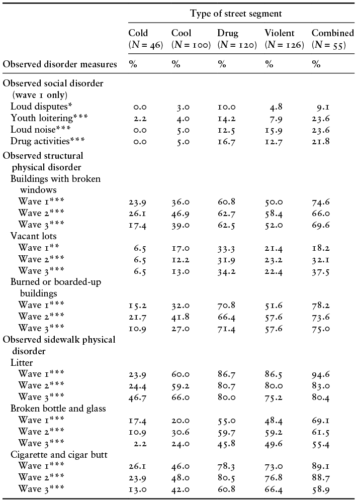
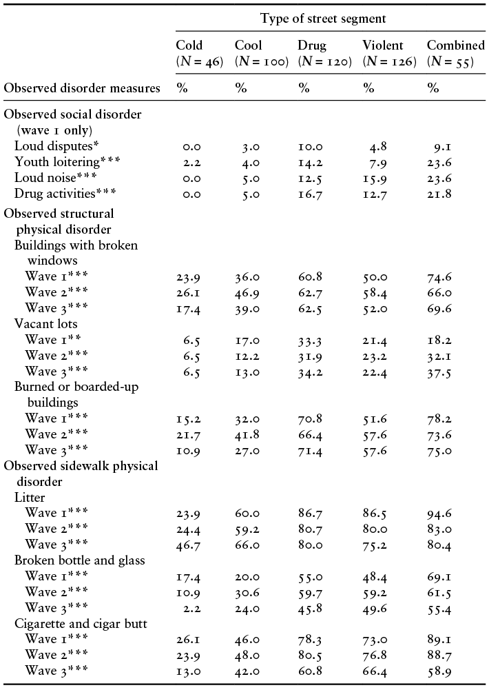
Applying the systematic social observation (SSO) method described in Chapter 1, we measured social disorder in wave 1. Drawing upon the physical observation (PO) data collection (see Chapter 1), we observed physical disorder on streets during each wave of the survey. Our findings provided in Table 2.8 suggest that it is not only crime, but also disorder more generally that is found on hot spot streets compared to cool or cold spots.

Table 2.8Individual measures of observed social and physical disorder by segment type

Note:

^* p ≤ 0.05, ^**p < 0.01, ^***p < 0.001; Outcomes represent the percentage of observers who reported presence of indicator at least once.

All four of our observational measures of social disorder show significant variability across the street types we studied. And in all cases the hot spot streets are much more likely to evidence social disorder than cool or cold spots and the differences are often large. For example, in more than 20 percent of the three twenty-minute observations we conducted on combined drug and violence hot spots in wave 1 of our study, our researchers identified loud noise, youth loitering, or drug activities. This was true for 5 percent or fewer of the cool spot streets, and in the case of loud noise or drug activities, there were no such events recorded by our observers on cold spot streets with little or no crime.

Overall, the drug hot spots and violent hot spots evidenced less social disorder than the combined drug/crime hot spots, but still much more social disorder than found in the cold and cool crime streets. In fact, in the qualitative visits to the streets, the field researchers often noted the lack of people outside on the cold and cool streets, whereas they experienced more foot traffic and street activity on the hot spots. This ranged from more prosocial behaviors such as neighbors sitting on porches visiting and kids playing basketball, to disorderly behavior indicators, such as young men standing around on corners or drug dealing. On one violent hot spot the field researchers noted that “there were a lot of people walking around, walking by, and on their porches and most of them said hello to us and asked how we were doing.” Alternatively, on a drug spot, the field researchers described apparent drug dealing activities –

a few people passed by – a man with scars on his neck who was on his phone, a couple of individuals with bags and money in their hand who did not make eye contact and did not seem to be fully aware of us when they passed by. Another three men came and walked by us, walking quickly, and counting a large amount of money openly.

The differences between hot spots and non–hot spots are even more pronounced for observed physical disorder. Across the three waves of our study, we examined structural physical disorder, such as broken windows, abandoned buildings, and burned or boarded-up buildings. We also had measures of sidewalk physical disorder, such as litter, broken bottles and glass, and cigarette or cigar butts on the street. All of these measures showed significant differences in all three waves of the study across the street types (see Table 2.8). And these differences are often dramatic. For instance, between 50% and 75% of the hot spot streets had buildings with broken windows, compared to only 17–26% of the cold spot streets and 36–47% of the cool spots. More than 50% of the hot spot streets had burned or abandoned buildings, whereas this was true for less than 22% of the cold spot streets and between 27 and 42% of the cool spots. Litter on the street was also observed on more than 75% of the hot spot streets, but only between 24% and 47% of the cold spots. Broken bottles or broken glass was observed on more than 45% of hot spot streets but on less than one-fifth of the cold spot streets, and most of the combined hot spots had visible cigarette/cigar butts, compared to 26% or fewer of cold spots.

Table 2.9Observed social and physical disorder factor scores by segment type

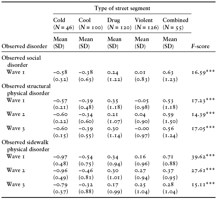
Note:

^*** p < 0.001; For all measures, means for wave 1, wave 2, and wave 3 = 0.

Our qualitative field researchers also observed notable differences in physical disorder across the different segment types, and it was expressed by residents in the qualitative interviews as well. The cold and cool spots were often described as having “little to no trash and the homes and yards being well cared for and maintained,” whereas on the hot spots the field researchers noted traditional indictors of disorder like lots of trash, broken glass, and boarded-up homes. One cold street was noted by one of the field researchers as having

flowers everywhere, decorated front lawns and stoops. It was the thing I noticed most about the street, the various colors of flowers and the plants growing in the front yards that seemed to have very specific designs and arrangements in each yard. There were steppingstones leading up to front doors, stones leading to backyards with statues, fountains, potted plants, and other decorations that all seemed to match some theme for each particular house.

Alternatively, a field researcher described a drug hot spot – “A few empty beer bottles were thrown on the walk side. Walk sides also contained untrimmed bushes. At least three empty lots were observed where no buildings are built, yet stairways are still there that link these empty lots to the main road. Trash was thrown in a couple of spots in the street.” On another drug hot spot, the field researchers wrote,

we noticed as soon as we stepped out of the car how dirty the neighborhood was. Trash was basically everywhere, broken furniture is thrown out at the corner of the street, as well as lots of beer bottles were thrown on both sides of the street. Although buildings are painted in different bright colors, they are damaged and neglected. Sewage water runs on the side of the street like a main water stream, leaving a bad smell for residents and passersby.

On a violent hot spot, researchers noted that “there are iron bars protecting the windows of the ground floor in all residential and commercial buildings. Dirt, trash, and food boxes were thrown on both sidewalks and in the middle of the street.” These passages highlight some of the more extreme cases, but demonstrate the wide variability in physical disorder across street types, and the often-stark differences between hot spot and cold spot streets.

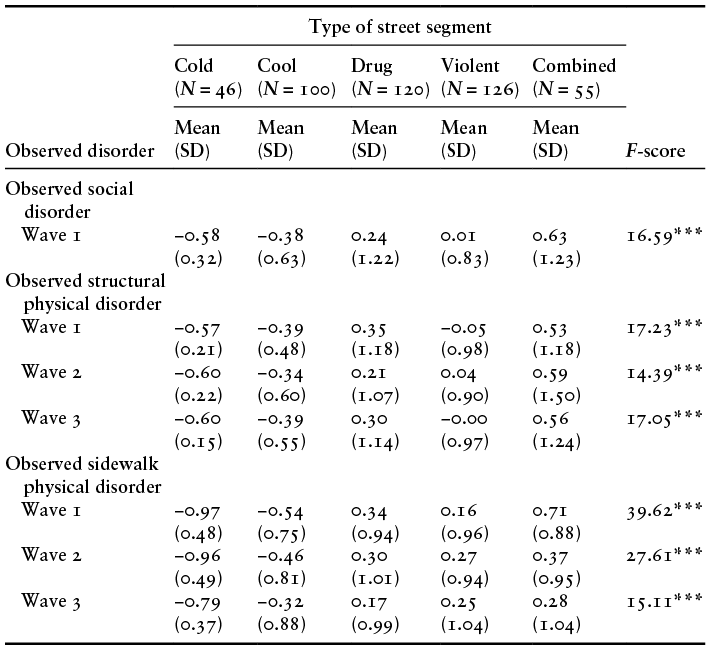
The clear patterns in individual measures are reaffirmed in three factor scores that consolidate these indicators into meaningful scales: observed social disorder, observed structural physical disorder, and observed sidewalk physical disorder.Footnote ⁸ As shown in Table 2.9, field researchers observed higher levels of social disorder, structural physical disorder, and sidewalk physical disorder on crime hot spots than cool and cold spots.

2.8.1.2 Perceived Disorder Measures

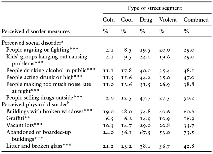
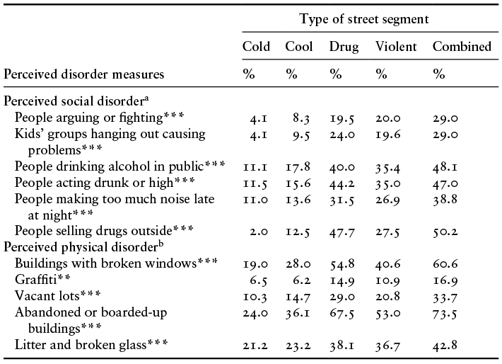
The patterns identified in observed disorder measures are also reflected in perceived disorder measures from the residential survey.Footnote ⁹ Table 2.10 demonstrates how residents perceive social and physical disorder on the streets by street segment type.Footnote ¹⁰ For all six types of social incivilities, residents’ perceptions vary significantly by street type. While fewer than 5% and 10% of residents in cold spots and cool spots, respectively, reported observing people arguing or fighting or groups of kids hanging out and causing problems a few times a week or every day, this figure rises to approximately 20 percent or more among residents of crime hot spots. Regarding measures such as people drinking alcohol in public, acting drunk or high, or making excessive noise late at night, residents in crime hot spots are at least twice as likely to report these types of disorder compared to those in cold and cool spots. Furthermore, observing people selling drugs on the streets is relatively common in hot spots, with 48% of residents in drug hot spots, 28% in violent hot spots, and 50% in combined hot spots reporting such activity a few times a week or every day, whereas such observations are rare in cold spots (2%) and less frequent in cool spots (13%).

Table 2.10Individual perceived social and physical disorder measures by segment type (wave 1)

Note:

^** p < 0.01, ^***p < 0.001;

^a = percent of residents who reported “a few times a week” or “everyday”;

^b = percent of residents who reported “one or two” or “many;” Ns are at the individual level and vary between 3,475 and 3,717 for the individual items.

Table 2.10 also highlights residents’ perceptions of physical disorder on the streets, which also vary significantly by street segment type. In cold and cool spots, respectively, fewer than 20% and 30% of residents reported observing buildings with broken windows, whereas this figure rises sharply to 55% in drug hot spots, 41% in violent hot spots, and 61% in combined hot spots. Similarly, reports of abandoned or boarded-up buildings are much higher in crime hot spots, with 68% in drug hot spots, 53% in violent hot spots, and 74% in combined hot spots noting their presence, compared to just 24% in cold spots and 36% in cool spots. Perceptions of residents regarding the presence of vacant lots also vary considerably, with only 10% of residents in cold spots and 15% in cool spots reporting them, compared to 29% in drug hot spots, 21% in violent hot spots, and 34% in combined hot spots. Graffiti, while less commonly observed by respondents overall, is more frequently reported in combined hot spots (17%) than in cold spots (7%) or cool spots (6%). Finally, reports of litter and broken glass are most likely to be observed by residents in combined hot spots (43%), followed by drug hot spots (38%) and violent hot spots (37%), while such issues are far less commonly observed in cold spots (21%) and cool spots (23%).

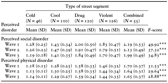
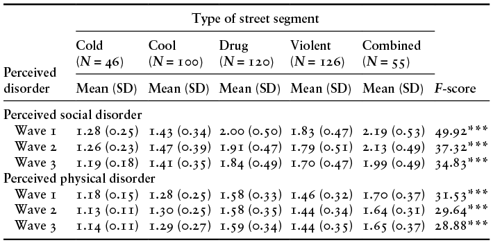
Regarding the mean scores for perceptions of social disorder, again, residents of crime hot spots report much higher levels of social disorder than those in non–hot spots (see Table 2.11). Among crime hot spots, the levels of disorder perceived by residents are the highest in combined hot spots, followed by drug hot spots and violent hot spots across all three waves.

Table 2.11Perceived social and physical disorder mean scores by segment type

Note:

^*** p < 0.001; For perceived social disorder, overall mean for wave 1, wave 2, and wave 3 are 1.77, 1.74, and 1.66, respectively; For perceived physical disorder, overall mean for wave 1, wave 2, and wave 3 are 1.45, 1.44, and 1.44, respectively.

Perceived physical disorder exhibits very similar patterns as those for perceived social disorder (see Table 2.11). Residents living in crime hot spots report much higher levels of physical disorder than those living in non–hot spots. Among different types of hot spots, residents of combined hot spots report the highest levels of disorder, followed by drug hot spots and violent hot spots. In the qualitative interviews, some residents’ accounts of the hot spots highlight the high levels of physical disorder that they perceive on these streets. One resident of a drug spot described the street as follows: “…when I first came to the area, it was so clean that you could even eat off the street, but now, look at the corners and see the trash…. Rats and insects are everywhere … people come from different areas to dump their trash and old furniture in our street” while pointing at an unattended broken sofa that was left at the corner of the street.

2.8.2 Fear of Crime

Perhaps the most direct consequence one might expect from living on streets with a great deal of crime would be fear of crime. Simply stated, when there are very high crime levels on a street, individuals would be expected to be more fearful about crime victimization (Brunton-Smith and Sturgis, Reference Brunton‐Smith and Sturgis2011; Kuen et al., Reference Kuen, Weisburd, White and Hinkle2022; Zhao et al., Reference Zhao, Lawton and Longmire2015). Fear, in itself, is a social ill, which has been linked to mental and physical health problems (Morrall et al., Reference Morrall, Marshall, Pattison and Macdonald2010; Stafford et al., Reference Stafford, Chandola and Marmot2007) and avoidance behaviors (Lane et al., Reference Lane, Rader, Henson, Fisher and May2014). Additionally, studies have demonstrated that fear of crime can weaken social integration among neighbors (Hinkle, Reference Hinkle2013) and lead to residents’ withdrawing from the streets they live on, which, in turn, results in more serious crime and disorder at those places (Skogan, Reference Skogan1990; Wilson and Kelling, Reference Wilson and Kelling1982).

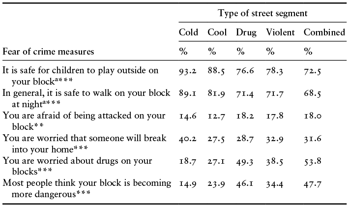
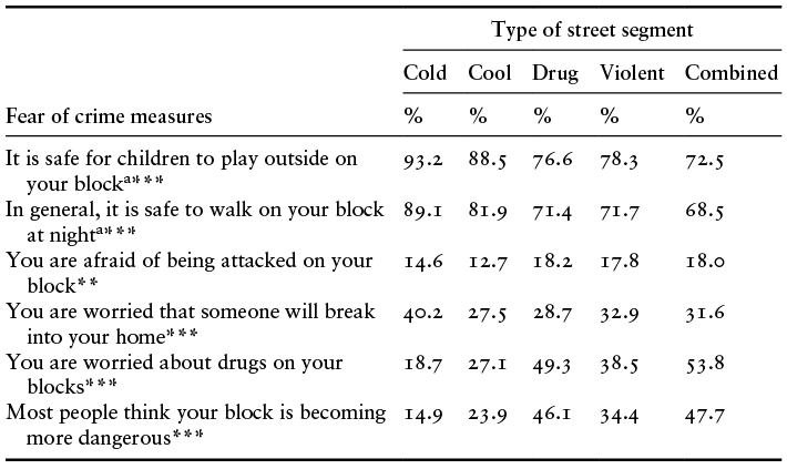
We measure fear of crime using six items that capture both cognitive and affective aspects of fear (Kuen et al., Reference Kuen, Weisburd, White and Hinkle2022; see also Markowitz et al., Reference Markowitz, Bellair, Liska and Liu2001).Footnote ¹¹ Similar to our approach with collective efficacy and disorder, we first assessed residents’ level of fear of crime for individual measures by street segment type in wave 1 (see Table 2.12).Footnote ¹² Overall, significant differences are evident across fear of crime measures, with residents of low-crime streets generally experiencing less fear than those on high-crime streets. An interesting exception is that residents of cold streets are more likely than those in hot spot streets to worry about someone breaking into their home. Perhaps this is the case because of the relatively advantaged economic situation on these streets, and the sense of residents that there is more to steal in their houses.

Table 2.12Individual fear of crime measures by segment type (wave 1)

Note:

^** p < 0.01, ^***p < 0.001; % = percentage of residents who reported “agree” or “strongly agree;” Ns are at the individual level and vary between 3,520 and 3,691 for the individual items; ^a = item was reversed coded for creating the mean scale.

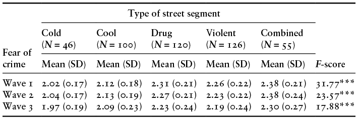
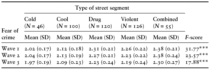
When examining the mean scale of fear of crime, we again find that fear of crime varies significantly across the streets, with residents of the hot spot streets having the highest levels of fear of crime (Table 2.13). There are relatively low levels of fear in the cold spots and cool spots in this case. As expected, hot spots of all types have higher levels of fear of crime than non–hot spots, though the differences among the types of hot spots are not very large and vary across the three waves of the study.

Table 2.13Fear of crime mean scores by segment type

Note:

^*** p < 0.001; Overall mean for wave 1 = 2.24, overall mean for wave 2 = 2.22, and overall mean for wave = 2.17.

In the qualitative interviews, residents of certain hot spots would speak of safety concerns and being fearful of crime, particularly for children or after dark. One female who lived on a drug spot said, “I am afraid, and I can’t allow my kids to be out after 8 pm, it’s too dangerous. Shootings and killings are happening continuously.” Another young woman living on a violent hot spot expressed, “my school friends won’t come to visit me at my house because they are afraid, and the area has a very bad reputation.” A woman who was visiting her sister on a violent hot spot also emphasized that she only visits her sister when it is daylight, “before 6 or 7pm at most.” A resident of a violent hot spot talked about wanting to move because of the crime and violence that took place. These concerns were not mentioned among the residents of the cold and cool spots.

2.9 Conclusions

In this chapter we have explored the social structure and social context of hot spot streets, and how they compare to non–hot spot streets. We have seen that hot spots of crime are not only hot spots of crime, but also hot spots of concentrated disadvantage, of low residential stability, of low informal social control, hot spots of social and physical disorder, and places of high levels of fear of crime. Our analyses in this chapter have not looked to establish causality among the characteristics we have examined, an issue we will address in later chapters. Rather, our purpose has been to provide a broader view of what hot spots are like and the kinds of social problems that are faced in these places. Understanding the social structure and social context of crime hot spots can help in understanding the broader problems faced by these places and how such problems can be overcome, an issue we return to throughout our book, and especially in our conclusions.

Our data also upend a common perception of hot spots of crime as uniformly chaotic and with little potential to exercise informal social control. Having detailed the tremendous challenges faced by people who live in crime hot spots, this should not lead us to believe that there is little to draw on in developing prevention and improvement schemes, an issue we will return to in the conclusions of our book. Despite high levels of concentrated social disadvantages on these streets, and relatively low levels of informal social control as compared with non–hot spots, we still observe meaningful levels of informal social control on hot spot streets. People who live on these streets are often willing to intervene in the life of the street, and they are often connected strongly to their neighbors. Indeed, we found little difference between the social networks and social ties reported on hot spot and non–hot spot streets. And in our qualitative interviews, people who lived on hot spot streets often talked with hope about their streets getting better in the future. These findings, in our view are as important as those that emphasize the distinctions between hot spot and non–hot spot streets, because they suggest a road map for how crime prevention can be achieved on hot spot streets, and the key importance of residents of those streets in that process. We return to this in detail when we discuss policy implications of our work in Chapter 8.