





1. Introduction
Glaciers are often noisy seismic environments, with a plethora of dynamic processes releasing seismic energy. Many of these source processes are of glaciological interest, so detection and subsequent interpretation of seismic recordings offer a valuable analysis toolbox. Such analysis is particularly pertinent for transient or subsurface processes, which often elude remote sensing techniques. Given the diversity of glaciated environments, relevant seismological methods differ according to the nature of the glacier or ice stream, and practicalities such as the size of the deployed seismic network relative to the glaciated area under investigation. Mountain glaciers provide a frequent focus of cryoseismic studies, due both to accessibility for methodology development (e.g. Walter and others, Reference Walter, Clinton, Deichmann, Dreger, Minson and Funk2009; Nanni and others, Reference Nanni, Roux and Gimbert2024), and for the livelihood and safety of surrounding communities (e.g. Eibl and others, Reference Eibl, Bean, Einarsson, Pàlsson and Vogfjörd2020). Using the suite of techniques developed across all glaciated environments, further reconnaissance is necessary for polar glaciers, particularly in the East Antarctic Ice Sheet (EAIS), where uncertainty remains on key glaciological processes (Noble and others, Reference Noble2020). In an EAIS context, apertures of arrays are often such that station separation is small compared to the source distance with large zones of seismicity, as opposed to mountain glacier studies (e.g. Nanni and others, Reference Nanni, Roux, Gimbert and Lecointre2022, Reference Nanni, Roux and Gimbert2024), and adaptations to methods must therefore be made.
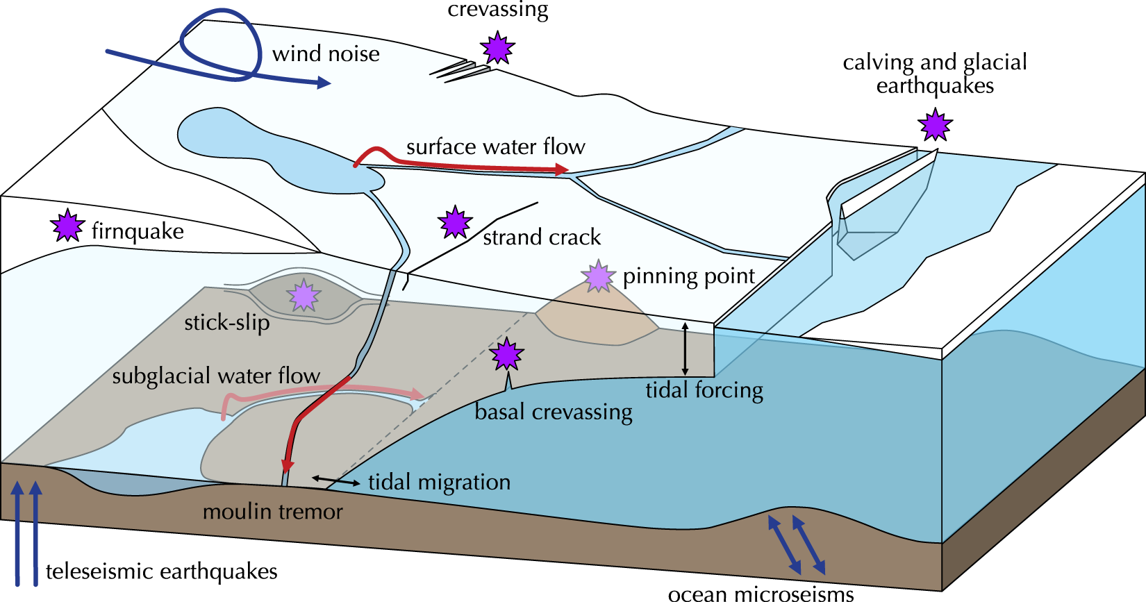
Cryoseismic events operate over a broad range of magnitudes, frequencies and durations (Podolskiy and Walter, Reference Podolskiy and Walter2016). For local observations of a single glacier or region therein, seismic recordings are typically dominated by small, high frequency ( $ \gt 1\,\mathrm{Hz}$) events from nearby sources, sometimes termed as glacier microseismicity (West and others Reference West, Larsen, Truffer, O’Neel and LeBlanc2010; Fig. 1). These sources are diverse and include fracture and fault-like mechanisms, sometimes referred to as ‘icequakes’ (purple stars in Fig. 1), as well as longer duration tremor sources (red arrows in Fig. 1). These signals from nearby glacier processes are superposed on other noise sources and distant events (blue arrows in Fig. 1).
Example seismic source mechanisms in an outlet glacier. Fracture and faulting mechanisms are denoted with purple stars. Tremor sources from flowing water are denoted with red arrows. Other external sources are indicated by blue arrows.

The earliest observations of icequakes were low magnitude events from surface crevassing (Neave and Savage, Reference Neave and Savage1970), in keeping with historical sensory observations that fracturing caused a sound and noticeable vibration in the ice. Surface crevassing has continued to be a focus of many cryoseismic studies, with mapping of crevasse fields (Roux and others, Reference Roux, Marsan, Métaxian, O’Brien and Moreau2008, Reference Roux, Walter, Riesen, Sugiyama and Funk2010), variations in surface conditions (Köhler and others, Reference Köhler, Maupin, Nuth and van Pelt2019; MacAyeal and others, Reference MacAyeal2019) and fundamental mechanistic understanding (Walter and others, Reference Walter, Clinton, Deichmann, Dreger, Minson and Funk2009; Hudson and others, Reference Hudson, Brisbourne, White, Kendall, Arthern and Smith2020) major points of interest.
Surface sources often have environmental drivers that influence the spatial and temporal distribution of events. The expansion and contraction of the surface ice with temperature fluctuations can induce thermal fracturing (Lombardi and others, Reference Lombardi, Gorodetskaya, Barruol and Camelbeeck2019; MacAyeal and others, Reference MacAyeal2019), and the pooling of surface water can leave the underlying ice vulnerable to hydrofracture (van der Veen, Reference van der Veen2007; Hudson and others, Reference Hudson, Brisbourne, White, Kendall, Arthern and Smith2020). Due to the proximity of the source to the surface, these events are typically characterised by dominant Rayleigh surface wave arrivals, which can be used to estimate the epicentral direction (Cooley and others, Reference Cooley, Winberry, Koutnik and Conway2019; Köhler and others, Reference Köhler, Maupin, Nuth and van Pelt2019), and characterise the shallow subsurface (Lindner and others, Reference Lindner, Laske, Walter and Doran2019).
Englacial and subglacial sources propagate seismic body waves through the interior of the glacier to the surface, and do not excite surface waves at the higher frequencies targeted in local studies due to the source depth. This distinction in seismic phase has been used to distinguish surface sources from those at depth (Deichmann and others, Reference Deichmann, Ansorge, Scherbaum, Aschwanden, Bernard and Gudmundsson2000; West and others, Reference West, Larsen, Truffer, O’Neel and LeBlanc2010; Hudson and others, Reference Hudson, Smith, Brisbourne and White2019). Englacial and subglacial sources are isolated from surface environmental forcing in the absence of an englacial hydrological system, but tidal stresses act throughout the interior of the glacier near the grounding line causing fracturing at the bed and surface alike with a tidal periodicity (Cooley and others, Reference Cooley, Winberry, Koutnik and Conway2019; Minowa and others, Reference Minowa, Podolskiy and Sugiyama2019; Olinger and others, Reference Olinger2019). Stick-slip events over subglacial asperities can also produce seismic signals from the glacier bed with tidal modulation (Zoet and others, Reference Zoet, Anandakrishnan, Alley, Nyblade and Wiens2012).
Glacier microseismicity can contain a long-duration tremor component. Perhaps the most widely studied of these is the tremor produced by the movement of meltwater, with this collection of sources sometimes referred to as glaciohydraulic tremor. The major components of this tremor are turbulence (Bartholomaus and others, Reference Bartholomaus, Amundson, Walter, O’Neel, West and Larsen2015), impacts of entrained sediments (Tsai and others, Reference Tsai, Minchew, Lamb and Ampuero2012), and resonance of the coupled fluid-solid system in moulins, fluid-filled cracks and pressurised cavities (St. Lawrence and Qamar, Reference St Lawrence and Qamar1979; Winberry and others, Reference Winberry, Anandakrishnan and Alley2009; Roeoesli and others, Reference Roeoesli, Walter, Ampuero and Kissling2016).
In addition to glacier microseismicity, large calving events can produce long-period ( $ \gt 30\,\mathrm{s}$) signals with durations on the scale of minutes, and can be recorded at regional and even global scales (Ekström and others, Reference Ekström, Nettles and Abers2003; Tsai and Ekström, Reference Tsai and Ekström2007; Nettles and Ekström, Reference Nettles and Ekström2010). Similarly, large stick-slip motions at Whillans Ice Stream produce long-period signals that can be detected at distances of over 1000 km (Winberry and others, Reference Winberry, Anandakrishnan, Wiens, Alley and Christianson2011). While these long-period events are present in the wavefield, they are vastly outnumbered by microseismic sources for the small-aperture installations used for local studies. As such, event catalogues are generally of high volume, with up to thousands of microseismic events occurring each day (Walter and others, Reference Walter, Roux, Roeoesli, Lecointre, Kilb and Roux2015; Köhler and others, Reference Köhler, Maupin, Nuth and van Pelt2019; Sergeant and others, Reference Sergeant2020).
In light of such large event counts, analysis techniques have been proposed that contrast with those used for small and well defined catalogues. Rather than a detailed treatment of individual events, a more statistical perspective of extracting trends in event rates, locations, and mechanisms has proved a more tractable approach. Some event types, such as stick-slip motion, have a consistent waveform expression that can be harnessed for detection and classification via cross-correlation template matching (Zoet and others, Reference Zoet, Anandakrishnan, Alley, Nyblade and Wiens2012; Köhler and others, Reference Köhler, Maupin, Nuth and van Pelt2019). For other event types where the seismic expression is less consistent due to variations in source mechanism or path effects, classification through clustering has proven fruitful (Jenkins II and others, Reference Jenkins, Gerstoft, Bianco and Bromirski2021; Hu and others, Reference Hu, Li, Fu and Liu2024; Latto and others, Reference Latto, Turner, Reading, Cook, Kulessa and Winberry2024a). Due to this complexity, developments for handling and extracting information from cryoseismic event catalogues, particularly for locating and classifying events, are crucial for advancing understanding of processes at polar outlet glaciers.
2. Data
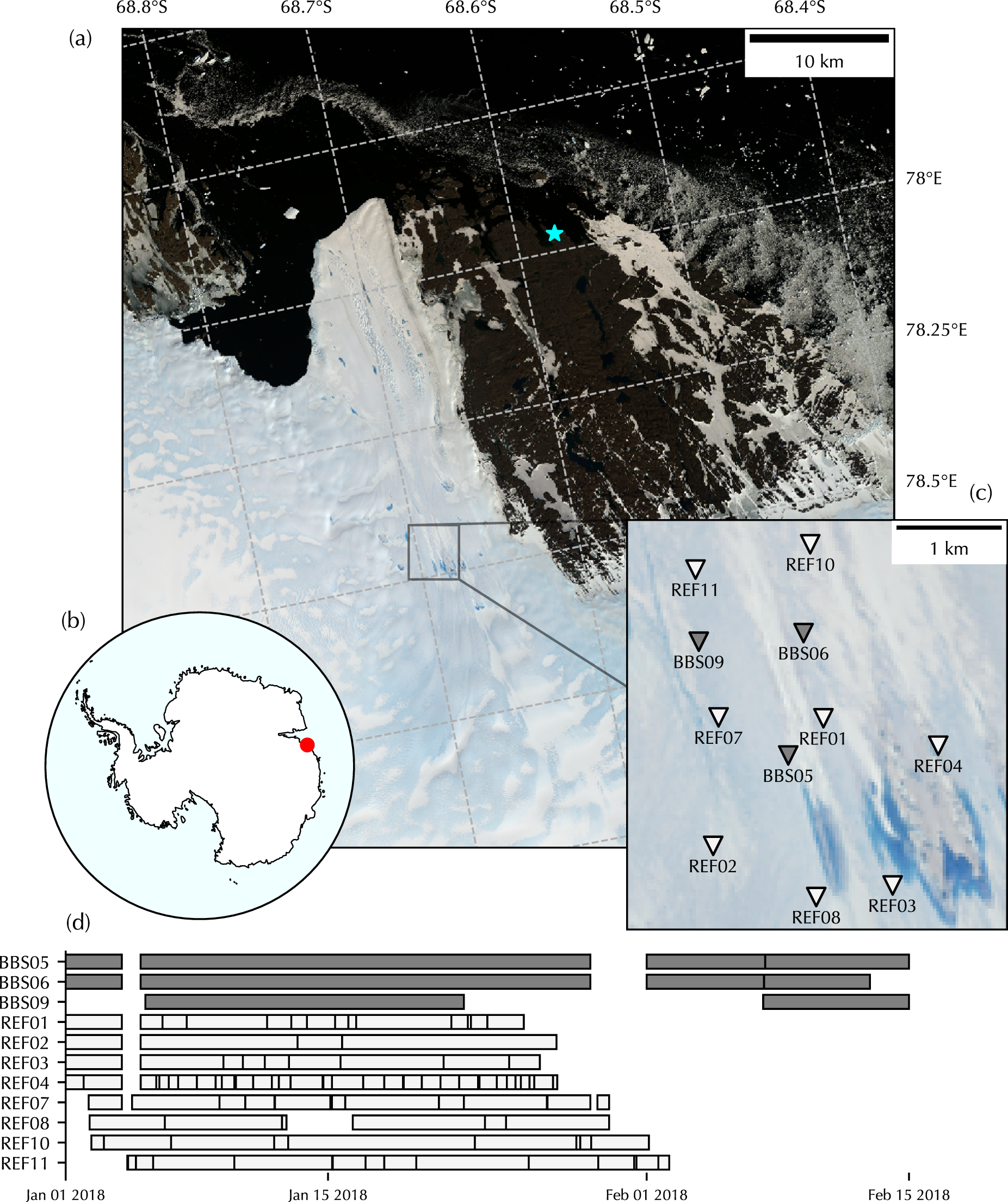
In this work, our focus is on characterising the seismicity of Sørsdal Glacier, East Antarctica from a deployment in the 2017–18 austral summer (Fig. 2). Located in Princess Elizabeth Land, Sørsdal Glacier is situated next to the Vestfold Hills and flows approximately westward to deposit ice from its calving front into Prydz Bay and, by extension, the Southern Ocean. A previous reflection seismic study near the site indicates an ice thickness of approximately 1400 m (Schaap and others, Reference Schaap, Roach, Peters, Cook, Kulessa and Schoof2020), and a grounding line position likely slightly downstream from the seismic array to give a floating ice shelf approximately 20 km long, and 8 km across at the widest points (Gwyther and others, Reference Gwyther2020).
(a) Map of Sørsdal Glacier study site with Davis Station marked (blue star). (b) Position of site (red circle) in Antarctic continent. (c) Seismic array comprising broadband seismometers (dark triangles) and short-period seismometers (light triangles). Satellite imagery of site on 25 January 2018 from Landsat 8. (d) Data availability for each of the seismic stations, with vertical lines indicating dropouts.

Sørsdal Glacier has a dynamic surface environment with supraglacial lakes and channels, crevassing and calving events at the terminus. Schaap and others (Reference Schaap, Roach, Peters, Cook, Kulessa and Schoof2020) identified englacial hydrological features that indicate movement of water between the surface and shallow subsurface, giving the possibility of glaciohydraulic tremor and signals associated with surface freeze-thaw cycles and hydrofracture. Sørsdal Glacier therefore provides an opportunity to investigate outlet glacier processes whilst testing a suite of seismological techniques in an EAIS setting.
The seismic installation consists of three broadband seismometers and eight short-period instruments, with positions indicated by the dark and light triangles, respectively, in Fig. 2, along with the data availability. The broadband instruments were Güralp CMG-40T seismometers with a natural frequency of 1 Hz and approximately flat response from 30 seconds, sampling at 100 Hz. The short-period instruments were OYO Geospace GS-11D geophones with a natural frequency of 4.5 Hz, connected to RefTek 130-01 data loggers sampling at 1000 Hz. Due to dynamic surface conditions, ground coupling was variable through the season, and data quality degraded later in the deployment.
To supplement the seismic data and identify environmental drivers for seismicity, surface temperature and tidal data are incorporated into this analysis. No in situ weather data were collected, so we instead use the automatic weather station (AWS) situated at the nearby Davis Station (blue star in Fig. 2). Tidal height is modelled using the CATS2008 model (Sutterley and others, Reference Sutterley2024), which is consistent with nearby tide gauges. All seismic results are reported in Coordinated Universal Time (UTC). Local time for Davis Station is UTC+07:00 for logistic convenience, but the longitude of the site gives a local solar time of UTC+05:12, which we use as a preferred reference for the AWS data.
3. Methods
We use the following workflow to extract information on cryoseismic event mechanisms. The methods used, summarised in the following steps, are outlined in the sections that follow.
(1) Produce a master event catalogue with the multi-STA/LTA algorithm of Turner and others (Reference Turner, Latto and Reading2021).
(2) Carry out spectral and temporal analysis of continuous seismic data and event occurrence.
(3) For each event in the master catalogue, calculate the backazimuth using matched field processing and polarisation analysis.
(4) Manually classify sections of data to form event groups, and select template events from each group.
(5) Use template matching to form secondary classified event catalogues.
(6) Calculate backazimuth and other seismic attributes (e.g. central frequency) for these classified catalogues to deduce potential source mechanisms and identify path effects.
Two catalogue types are therefore produced through this methodology: the initial master catalogue for understanding the overall seismicity of the glacier, and the classified catalogues from template matching for understanding trends in particular event types.
3.1. Event detection
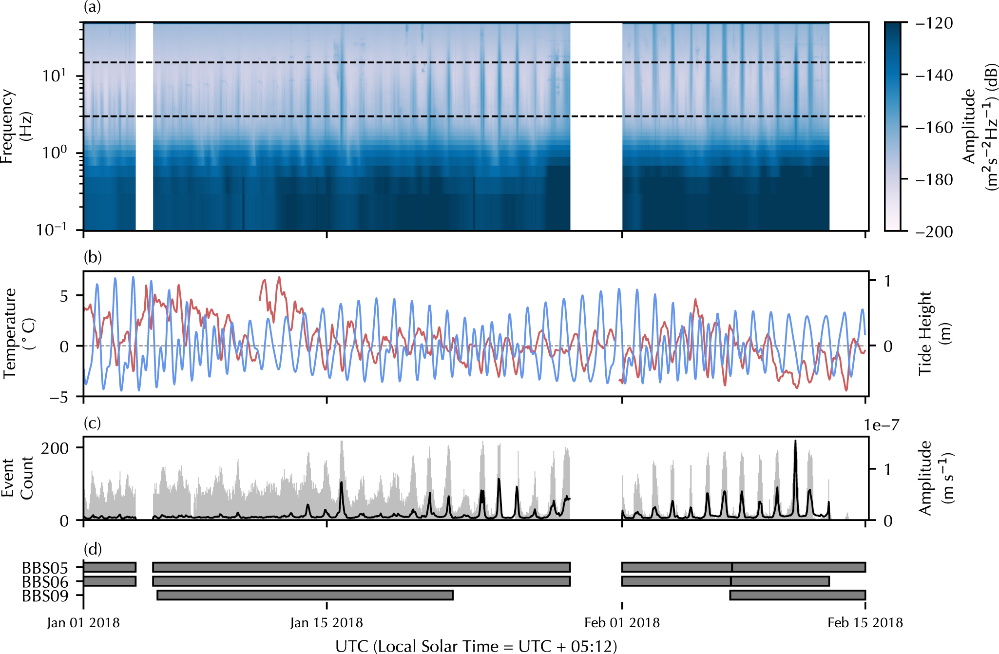
To characterise the seismic source mechanisms at Sørsdal Glacier, we first produce an initial master event catalogue. This is designed to capture the broad diversity of event mechanisms with correspondingly diverse waveforms. It can be used to discern trends in the overall seismicity of the glacier (Fig. 3), but remains agnostic to trends in source type and location; factors that are further considered in the following sections.
(a) Median spectrogram for the vertical component of BBS06, with dashed lines marking 3–15 Hz frequency band. (b) Modelled tides at Sørsdal ice shelf (blue) and air temperature (red) at Davis Station. (c) Number of events detected in each window (grey histogram) and median seismic amplitude (black solid line) for BBS06 vertical component in 3–15 Hz frequency band. (d) Data availability at each of the broadband stations.

A short-term-average/long-term-average (STA/LTA) triggering algorithm is used to detect seismic events. The optimal choices of sliding window lengths for the short- and long-term averages in traditional STA/LTA triggering are dependent on the duration and dominant period of the events of interest. We use the multi-STA/LTA variant of Turner and others (Reference Turner, Latto and Reading2021) to relax this prior knowledge constraint and allow multiple window lengths to be used and capture events with durations and frequencies across multiple orders of magnitude.
For consistency in instrument type, only the three broadband seismometers are used for the event detection step. A bandpass filter with cosine corner frequencies of 1, 2, 45 and 50 Hz is applied to remove ocean microseism energy and isolate the band where microseismicity dominates (Podolskiy and Walter, Reference Podolskiy and Walter2016). The Euclidean norm of the three components of motion is taken at each station to give the absolute amplitude, and the trigger detection is applied to this combined component so that events dominated by either horizontal or vertical motion can be detected. This absolute amplitude is only used for event detection, with the original three-component data used for subsequent event analysis.
The minimum window lengths for the short- and long-term averages are 0.2 and 2 seconds, respectively. The longer window pairs are multiplicative steps of 2 from these lengths that are capped at maximum lengths of 10 and 100 seconds. Triggers are then assigned based on when any of these STA/LTA ratios exceed a threshold of 4, and detriggers when the ratio drops back below 3. These trigger threshold values and window lengths were manually tuned for the dataset to minimise false detections and ensure that events were cropped at an appropriate duration.
To further minimise false detections and only include events captured across the array, at least two of the three broadband stations must have triggered within the time that the slowest seismic wave was expected to travel across the network, and selected to be a conservative Rayleigh wave velocity of 1.5 km s $^{-1}$. This simple association algorithm was suitable for the small aperture installation as the instruments were sufficiently close together to limit overlapping of events with different sources and thus incorrect association of triggers.
For each event, a duration, amplitude and central frequency are computed. The duration is defined as the time between the trigger-on and trigger-off of the multi-STA/LTA algorithm. The amplitude is the maximum absolute three-component amplitude recorded across broadband stations for the event. The central frequency is the mean value of the power spectrum for the vertical component at the station with the maximum amplitude. These three attributes give a brief summary of the waveform properties of an event.
3.2. Spectral and temporal analysis
To aid in the interpretation of the event catalogue and identify continuous tremor sources, median spectrograms are computed to further characterise the seismicity (Bartholomaus and others, Reference Bartholomaus, Amundson, Walter, O’Neel, West and Larsen2015). Power spectral densities (PSDs) are computed at each station for 5 second sliding windows with 50% overlap and a Blackman taper. The median of these 5 second PSD samples is then taken at each frequency within hourly bins to yield a single PSD for each hour of the deployment at each station. To assess any continuous glaciohydraulic tremor, we integrate the median spectrogram over the 3–15 Hz frequency band with this or a similar band often used as a proxy for subglacial water discharge (Bartholomaus and others, Reference Bartholomaus, Amundson, Walter, O’Neel, West and Larsen2015; Gimbert and others, Reference Gimbert, Tsai, Amundson, Bartholomaus and Walter2016; Lindner and others, Reference Lindner, Walter, Laske and Gimbert2020).
We consider two candidate environmental drivers for seismic activity: surface air temperature, which can alter the surface seismicity through meltwater availability and thermal stresses; and tidal height, which can influence the internal stresses through the rise and fall of the ice shelf. To elucidate the effects of these cyclic drivers on seismic recordings, periodic wrapping methods are used.
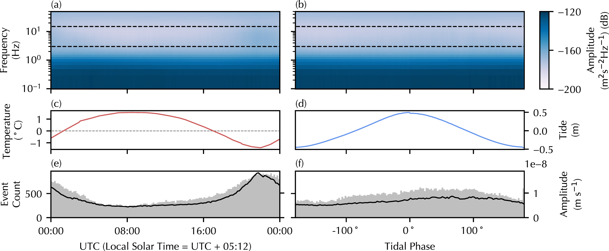
To identify diurnal patterns, a median spectrogram is produced by binning over time-of-day. The 5 second PSDs used to construct the full spectrogram (Fig. 3) are assigned to 10 minute bins based on time since 00:00:00 UTC, with the median again taken within each bin (Fig. 4). This is similar to the method of McNamara and Buland (Reference McNamara and Buland2004), but taking the median at each frequency rather than the mode. A tidal spectra is constructed using a similar method. The tidal phase is estimated for each of the 5 second PSDs by assigning  $\pm 180^\circ$ to low tide and $0^\circ$ to high tide, and linearly interpolating between these phases. The PSDs are then binned according to tidal phase into $2.5^\circ$ bins, and the median is taken at each frequency (Fig. 4). Each event in the catalogue is also assigned a time-of-day and tidal phase using the same method, and the event counts are binned into diurnal and tidal cycles to identify trends in impulsive event rates with respect to the environmental drivers.
(a and b) Median spectrograms with diurnal (a) and tidal (b) wrappings. (c) Mean surface temperature at Davis Station wrapped diurnally. (d) Mean tide height from CATS2008 with tidal wrapping. (e and f) Event count (grey histogram) and median velocity in 3–15 Hz band with diurnal (e) and tidal (f) wrapping.

3.3. Backazimuth estimation
Along with event timing, source locations can be used to aid in the assignment of potential mechanisms. Constraining epicentral distance is a challenging task for seismic installations such as this, where most events occur outside of the network. We can, however, provide some estimates of event backazimuth relative to the network centre as an indication of event location. Two methods are applied: matched field processing (MFP) and a form of polarisation analysis; the second of which is novel for multiple stations in the glacier setting.
3.3.1. Matched field processing
We could not identify any events in this catalogue that were dominated by clear body wave arrivals, so travel time inversion was not attempted. We elected to use array processing, which is a popular choice when working with signals without clear phase arrivals and when source locations are outside of the installation. Beamforming is one such processing method that has been successfully used in cryoseismic studies (e.g. Winberry and others, Reference Winberry, Anandakrishnan and Alley2009; Cooley and others, Reference Cooley, Winberry, Koutnik and Conway2019; Lindner and others, Reference Lindner, Laske, Walter and Doran2019). However, the aperture of the array used here is sufficiently large that many events violate the underlying planar wavefront assumption. We therefore use MFP, which propagates curved wavefronts, and therefore produces more accurate results for sources within or near the array, whilst the method converges to the planar beamforming case in the far-field. MFP is a task of maximising seismic signal coherence across the stations over candidate source locations. The method was originally developed for locating noise sources in ocean acoustics (Bucker, Reference Bucker1976), but now also widely used in array seismology (Gal and others, Reference Gal, Reading, Rawlinson and Schulte-Pelkum2018), and increasingly in cryoseismology (Walter and others, Reference Walter, Roux, Roeoesli, Lecointre, Kilb and Roux2015; Lindner and others, Reference Lindner, Walter, Laske and Gimbert2020; Sergeant and others, Reference Sergeant2020; Köhler and others, Reference Kohler, Myklebust and Mæland2022; Nanni and others, Reference Nanni, Roux, Gimbert and Lecointre2022).
A six-second window commencing two seconds before the first station trigger time is taken for analysis of each event, with this window length representative of a typical event duration. For this window, the frequency spectrum  $\mathbf{X}(f)$ is found for the vertical component of each of the short-period stations (light triangles in Fig. 2), which are exclusively used in this step due to their greater number compared to the broadband instruments. This spectrum is then trimmed to the 3–10 Hz frequency band where a majority of the Rayleigh wave energy is concentrated, and the instrument response is removed. While there are events in the catalogue with energy at higher frequencies, these frequencies lack the necessary coherence across the array due to attenuation, and most events detected still contain some energy within the 3–10 Hz band, even if it is not the spectral peak. Furthermore, a low-frequency band is more computationally efficient for MFP as the inclusion of shorter wavelengths would require a much denser grid spacing for resolving constructive and destructive interference.
For a given frequency bin of the spectra, the cross-spectral density matrix  $\mathbf{K}(f)$ is defined by
 \begin{equation}
\mathbf{K}(f) = \mathbf{X}(f)^\dagger \mathbf{X}(f),
\end{equation}
\begin{equation}
\mathbf{K}(f) = \mathbf{X}(f)^\dagger \mathbf{X}(f),
\end{equation}where  $\mathbf{X}(f)^\dagger$ represents the conjugate transpose of the spectrum. For $N$ stations, (1) is an $N \times N$ matrix for each discrete frequency, and only needs to be computed once for each event. For a homogeneous, non-dispersive medium, the steering vector, $\mathbf{d}(f)$, is given by
 \begin{equation}
\mathbf{d}(f) = \exp\left(-2\pi i f \mathbf{r} s\right),
\end{equation}
\begin{equation}
\mathbf{d}(f) = \exp\left(-2\pi i f \mathbf{r} s\right),
\end{equation}where  $\mathbf{r}$ is an $N$ element column vector that is the horizontal distance from the source to each of the stations, and $s$ is the horizontal slowness. The steering vector encapsulates the geometry of the array by applying the phase shift associated with the travel time between a proposed source location and each of the stations. The coherence at frequency $f$ across the array for a particular grid-point can be measured using the Bartlett processor:
 \begin{equation}
B(f) = \left|\mathbf{d}(f)^\dagger \mathbf{K}(f) \mathbf{d}(f)\right|.
\end{equation}
\begin{equation}
B(f) = \left|\mathbf{d}(f)^\dagger \mathbf{K}(f) \mathbf{d}(f)\right|.
\end{equation}This is averaged across the 3–10 Hz frequency band to give a coherence value for the proposed source location and slowness value.
For each event, a grid search is performed over backazimuth, epicentral distance and horizontal slowness. The backazimuth grid consists of 50 linearly spaced points through all angular directions. The radial grid is 50 log-2 spaced points from  $2^{-5}$ km ( $\sim 0.03$ km) to $2^{4}$ km ( $16$ km), giving a similar spatial grid geometry to Almendros and others (Reference Almendros, Ibáñez, Alguacil and Del Pezzo1999). As we are targeting surface Rayleigh waves, the horizontal slowness is the reciprocal of the wave velocity. To capture this range of Rayleigh wave velocities in glacial ice, a linearly spaced grid of 50 points between 1.4 km s $^{-1}$ and 2.3 km s $^{-1}$ is used. We then use the Nelder–Mead simplex algorithm for further refinement with initialisation at the optimal grid search solution; however, in most cases, the refinement only slightly changes the estimate.
3.3.2. Polarisation analysis
To supplement the MFP result, we also use polarisation analysis to give an additional backazimuth estimate. Polarisation methods are frequently used when there is a limited number of sensors as a single three-component record is sufficient to estimate event backazimuth if a seismic phase can be isolated. Many such methods use an eigenvector decomposition to derive planes of motion from the three-component recordings (Jurkevics, Reference Jurkevics1988). However, at this site, the signals are dominated by Rayleigh waves, particularly in the 3–10 Hz frequency band analysed for MFP. At the surface, Rayleigh waves produce retrograde elliptical particle motion in the vertical source-receiver plane. As a result, the radial component of motion is correlated with the vertical component with a  $\pi/2$ phase shift applied, termed the Hilbert transform. Baker and Stevens (Reference Baker and Stevens2004) harnessed this to show that backazimuth relative to a single station can be estimated by rotating the horizontal components through a range of backazimuth values to maximally correlate the radial motion with the phase-shifted vertical motion. That is, we seek the backazimuth that maximises
 \begin{equation}
\rho_j = \frac{\sum_{i=1}^T \left(v_R^{(j)}(t_i)\right)\left( \mathcal{H}[v_Z^{(j)}](t_i)\right)}{\sqrt{\left(\sum_{i=1}^T v_R^{(j)}(t_i)^2\right)\left(\sum_{i=1}^T \mathcal{H}[v_Z^{(j)}](t_i)^2\right)}},
\end{equation}
\begin{equation}
\rho_j = \frac{\sum_{i=1}^T \left(v_R^{(j)}(t_i)\right)\left( \mathcal{H}[v_Z^{(j)}](t_i)\right)}{\sqrt{\left(\sum_{i=1}^T v_R^{(j)}(t_i)^2\right)\left(\sum_{i=1}^T \mathcal{H}[v_Z^{(j)}](t_i)^2\right)}},
\end{equation}where  $v_R^{(j)}$ and $v_Z^{(j)}$ are the radial and vertical velocity components, respectively, at the $j$-th seismometer, $\mathcal{H}$ represents the Hilbert operator and $t_i$ for $i=1,2,...,T$ are the time samples within the window.
To make use of all three broadband stations (see dark triangles in Fig. 2) in a combined estimate, we aim to find a source location that simultaneously maximises the correlation across all stations. This requires a search over a 2D spatial grid, with a prospective source location yielding a different backazimuth for each station. For consistency in the ensuing comparison, we use the radial grid defined for MFP and the 3–10 Hz frequency band for a six-second window commencing two seconds before the trigger time.
One method for computing the combined correlation would be to sum the correlation contribution (4) from each of the broadband stations. However, these individual correlations are normalised to lie in the range -1 to 1, regardless of the energy of the signal. To prioritise the stations recording higher energy signals, we instead consider the combined correlation
 \begin{equation}
\rho = \frac{\sum_{j=1}^N\sum_{i=1}^T \left(v_R^{(j)}(t_i)\right) \left(\mathcal{H}[v_Z^{(j)}](t_i)\right)}{\sqrt{\left(\sum_{j=1}^N\sum_{i=1}^T v_R^{(j)}(t_i)^2\right)\left(\sum_{j=1}^N\sum_{i=1}^T \mathcal{H}[v_Z^{(j)}](t_i)^2\right)}},
\end{equation}
\begin{equation}
\rho = \frac{\sum_{j=1}^N\sum_{i=1}^T \left(v_R^{(j)}(t_i)\right) \left(\mathcal{H}[v_Z^{(j)}](t_i)\right)}{\sqrt{\left(\sum_{j=1}^N\sum_{i=1}^T v_R^{(j)}(t_i)^2\right)\left(\sum_{j=1}^N\sum_{i=1}^T \mathcal{H}[v_Z^{(j)}](t_i)^2\right)}},
\end{equation}which amounts to concatenating the radial and Hilbert transformed vertical components from each station into single vectors prior to computation of the correlation coefficient. As with MFP, the maximised grid point is used as an initial point for local optimisation with the Nelder–Mead algorithm.
3.4. Event classification
Due to the range of seismogenic mechanisms in a glacier, the events within the catalogue must be separated into groups of similar appearance to better identify potential mechanisms. We first manually analyse small sections of the catalogue to characterise dominant event types, and then extend this analysis to the full dataset using templates selected from the analysed segments.
3.4.1. Manual analysis
Three time windows, each 8 hours long, are manually analysed to identify some of the commonly recurring seismic event types operating at this site. To cover different periods in the season and times of day, these windows were selected to be January 8 (00:00-08:00 UTC), January 14 (16:00-00:00 UTC) and January 20 (08:00–16:00 UTC). Data quality for the broadband instruments was seen to degrade throughout February with increasing noise levels, so manual analysis was not attempted for a later time window. We therefore do not expect the selected templates from January to be fully applicable later in the season.
To provide an initial basis for classification, eight groups are formed by visual inspection and assignment. False detections are left unassigned, as are events that do not fit well with any of the group descriptions. As event templates are formed from these groups, many events are left unclassified to ensure that all events within these classified groups have an appropriate level of self-similarity and an adequate signal-to-noise ratio to be effective templates.
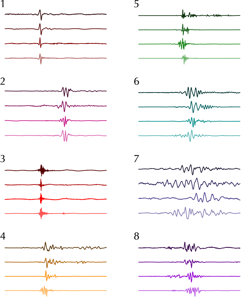
Four events from each of the eight groups are then selected to act as template events (Fig. 6). To make sure these templates are well-representative of the group, cross-correlation hierarchical clustering is applied within each group and templates selected from events that are central to the dominant clusters.
3.4.2. Expansion of classification
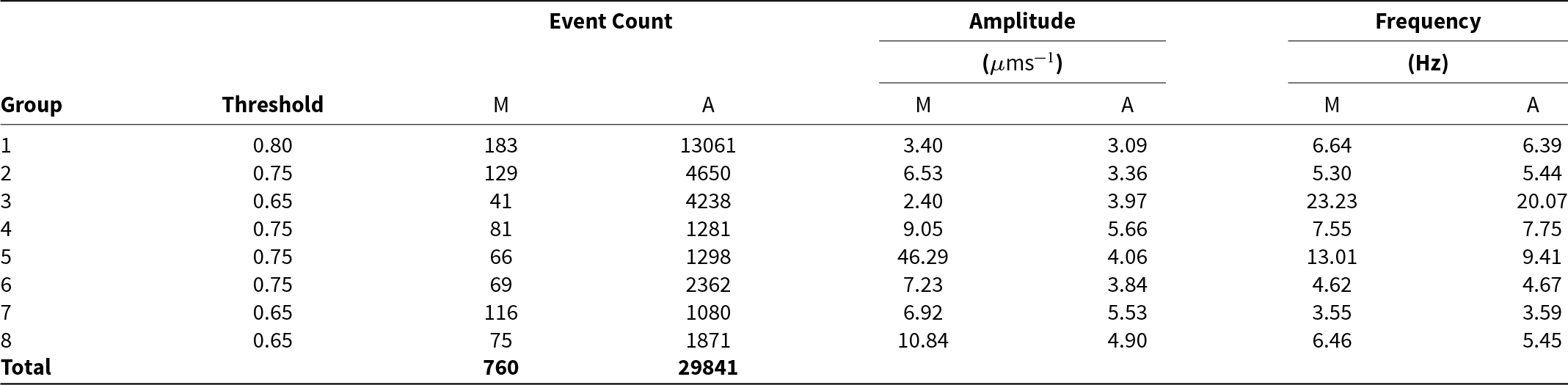
A template matching method is used to form secondary event catalogues corresponding to each group, which can be used to extract temporal and spatial trends. The cross-correlation is computed between the template waveforms and the continuous data belonging to the same station. That is, we do not compute correlations between the template at one station with the data at another. Peaks in cross-correlation correspond to lag times that align the template with other times of similar ground motion, and when the cross-correlation exceeds a given threshold for the template (Table 1), a detection is assigned based on this lag time with a minimum of 10 seconds between detections. As this detection is associated with the template used, the event is added to the corresponding secondary catalogue, and thus the method simultaneously detects and classifies events.
Tabulation of manual and automated classification groups. Group numbers correspond to template groups visualised in Fig. 6. The median of the amplitude and frequency for each group is shown. Columns labelled M and A refer to the manual and automated groups, respectively.

4. Results
4.1. Seismicity of Sørsdal Glacier
The 69,158 events included in the master catalogue (Section 3.1) are displayed in Fig. 3, along with the median spectrogram (Section 3.2), and potential environmental drivers of air temperature and tidal height. The event rate is variable across the duration of the deployment, and has a notably strong cyclic nature. To determine the nature of this periodicity, wrapped spectrograms and event rates with respect to time-of-day and tidal phase (Section 3.2) are displayed in Fig. 4.
Similar to MacAyeal and others (Reference MacAyeal2019), diurnal and tidal cycles are difficult to disentangle across the short duration of this study, as the period of each cycle is similar, so not all combinations of time-of-day and tidal phase were observed or equally sampled. However, the spectra in Fig. 4 suggest that a diurnal cycle more strongly influenced the event occurrence and seismic energy for this time period.
4.2. Spatial distribution
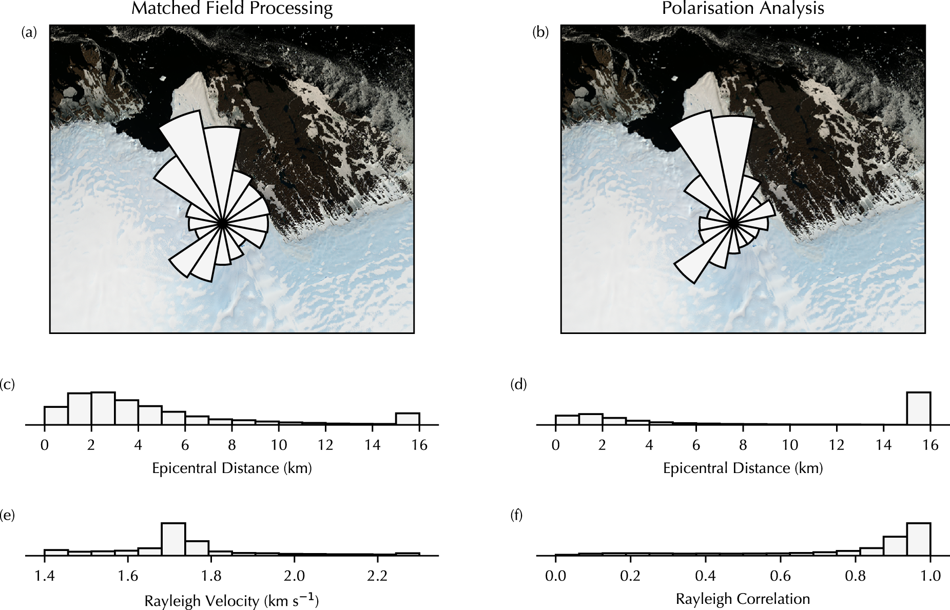
The MFP method is applied to all events in the catalogue where short-period data are available, and the polarisation analysis to all events with broadband data to produce the backazimuth estimates, along with corresponding epicentral distances, Rayleigh wave velocities, and correlation coefficients in Fig. 5. Due to the positioning of most events outside of the array, the epicentral distances, particularly from polarisation, are subject to too much error for any definitive interpretation.
(a and b) Backazimuth distribution for (a) matched field processing and (b) polarisation analysis. (c and d) Epicentral distance estimate for (c) matched field processing and (d) polarisation analysis. (e) Optimised Rayleigh wave velocity distribution from matched field processing. (f) Optimised Rayleigh coefficient (5) for polarisation analysis.

The Rayleigh wave velocities are consistent with those expected in ice for this frequency range (Lindner and others, Reference Lindner, Laske, Walter and Doran2019), and the correlation coefficients are generally high. The Rayleigh wave assumptions and selected frequency band, therefore, appear justified for these analyses, and further confirm that near-surface sources are the major component of seismicity at this site.
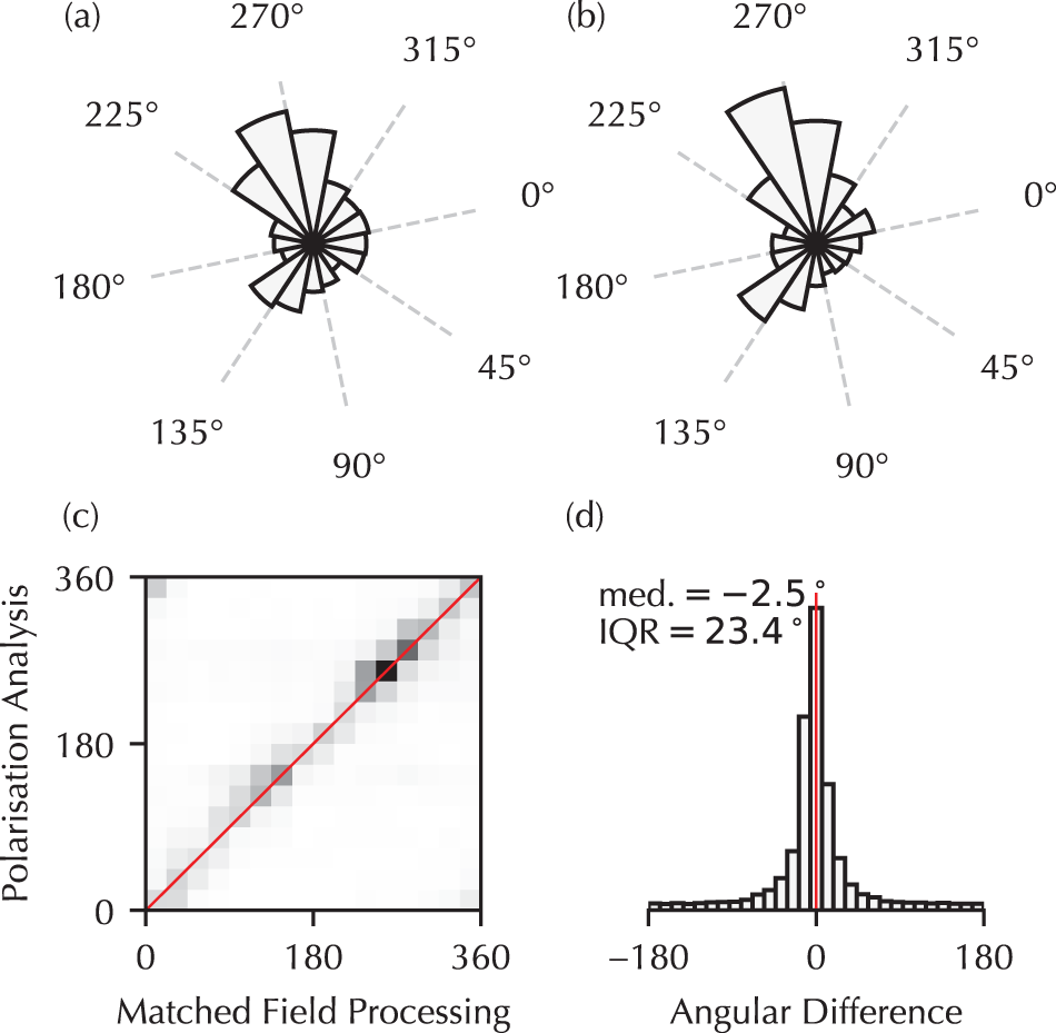
Both methods are in general agreement that most events are located downstream of the deployment, with an additional lateral peak in the South-East direction. There is no clear systematic bias, with a roughly symmetrical angular difference distribution in Fig. 7 and median value of  $-2.5^\circ$. However, the interquartile range of $23.4^\circ$ indicates there is still disagreement on many individual events. This exemplifies the difficulty in producing accurate, or even consistent estimates of event location for a deployment of this type. We are therefore mainly seeking qualitative information from these computations rather than exact locations. As such, both methods are sufficient, and in agreement, on qualitative backazimuth information, such as whether an event originates from upstream, downstream, or lateral to the ice flow.
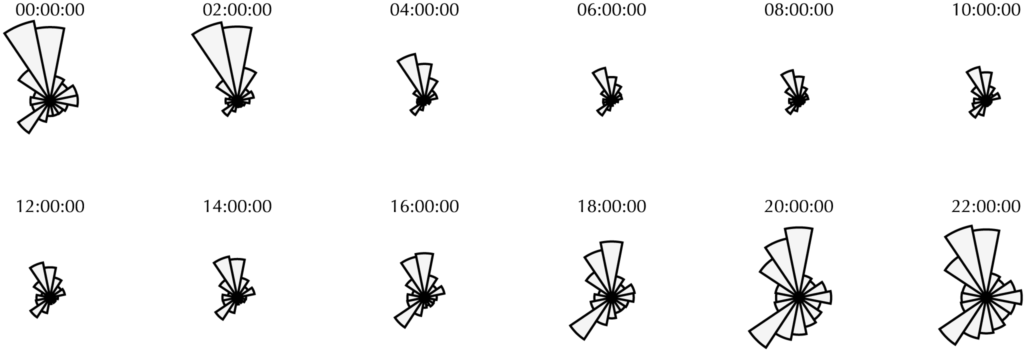
The event timings and backazimuth estimates can be combined to provide insights on the spatio-temporal distribution of events. Figure 8 shows the polarisation backazimuth distribution split into two hour bins according to time-of-day. It can be seen that the downstream lobe operates in near-isolation from 00:00:00 to 04:00:00 UTC while it and the lateral peak are of a similar size for 18:00:00 to 00:00:00 UTC.
4.3. Template matching
For the manual classification described in Section 3.4.1, 666 events were analysed for January 8 00:00-08:00 UTC (false detection rate of 9%), 999 events for January 14 16:00-00:00 UTC (false detection rate of 22%) and 342 events for January 20 08:00–16:00 UTC (false detection rate of 23%). The false detection rate, therefore, rose throughout the manual analysis due to degradation in data quality, but we note that these rates are higher than the true false detection rate, as events where stations had poor data quality or a lack of coherence between stations are included, even if it were a potential event.
The 32 templates representing the eight event groups selected from the manual analysis outlined in Section 3.4.1 are shown in Fig. 6, and provide an indication of the waveform characteristics used to define each group. Note that only the vertical component from the station with the greatest amplitude is shown, but the vertical components from all broadband stations are used for the template matching.
Vertical component event templates for each manually assigned group. All displayed traces are 6 seconds in length.

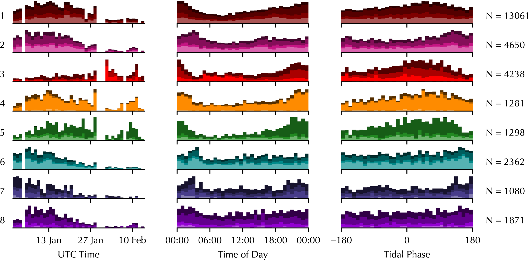
A total of 29,841 events are detected and thus classified into the eight event groups using the correlation detector. A summary of these groups and the typical amplitude and frequency are shown in Table 1. The cross-correlation threshold for each group is also given, with this tuned according to the expected similarity of waveforms within each group.
The central frequency of the automatically and manually classified events is similar, as frequency is a key factor influencing the ‘shape’ of the waveform. However, we see that the amplitude of the automatically classified events often differs from the manual groups. There are two factors at play here. Firstly, the cross-correlation is independent of amplitude, so manual groups such as Group 5 that are classified largely on amplitude are not expected to be matched well with this method. Secondly, the manual groups are formed using only events with high signal-to-noise ratios to ensure they can be strong candidate templates, and consequently often have a higher amplitude than the overall population of events.
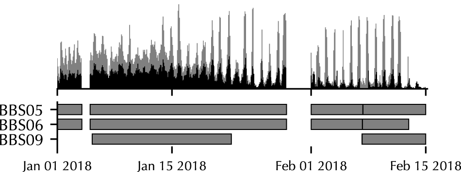
The multi-STA/LTA catalogue contained more events than the secondary classified catalogues, owing to the greater diversity of event types allowed with an amplitude-based trigger, with Fig. 9 overlaying the event distributions of the two catalogues. We also see that fewer events were detected later in the season with the template matching method. Recall that the template events were only drawn from earlier in the season due to lower data quality through February, so the combination of evolving event types and high noise levels lessens the effectiveness of the template matching. Aside from this lowered detection rate later in the deployment, the trends in seismicity are consistent between the two catalogues, and we can be confident that the two algorithms are triggering on approximately the same events. The distribution of events within each of the template groups is shown in Fig. 10, with absolute time, time-of-day and tidal phase distributions shown.
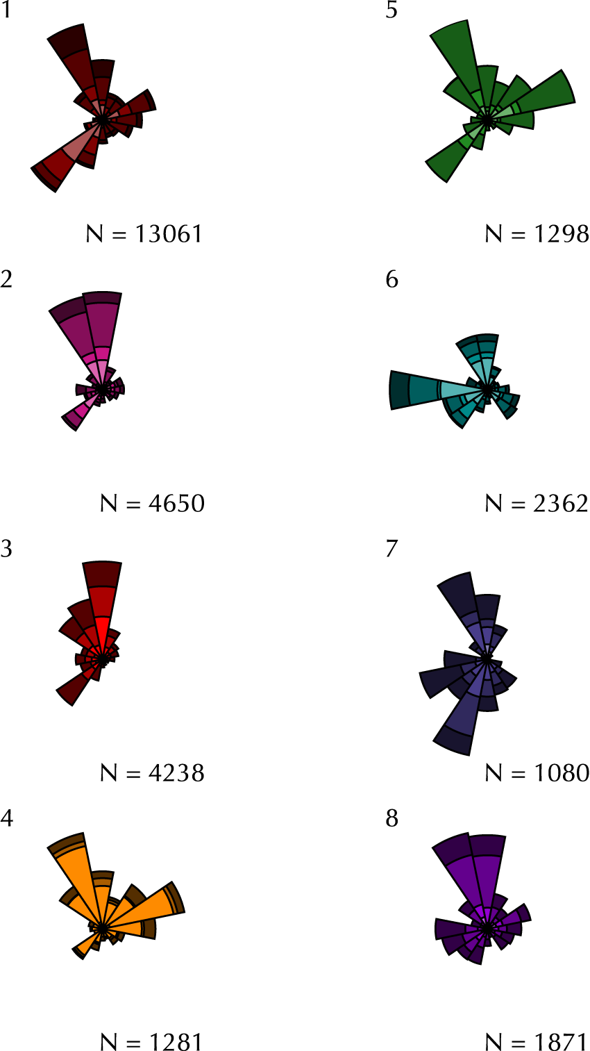
The backazimuth is again estimated for the events in this classified catalogue, with both the polarisation and MFP methods applied. The polarisation backazimuth estimates for each of the groups are visualised in Fig. 11. MFP produced similar spatial patterns, as was seen in Figs. 5 and 7. We therefore include only the polarisation result here due to the broadband data having greater availability, and thus giving results for the entire classified catalogue.
(a and b) Backazimuth estimates for (a) matched field processing and (b) polarisation analysis, for events where both estimates are available. (c) Bivariate distribution of the matched field processing and polarisation backazimuth estimates with perfect agreement indicated (red line). (d) Distribution of the difference between backazimuth estimates (MFP minus polarisation), with perfect agreement indicated (red line).

5. Discussion
There are two main facets for discussion of the results: the glaciological implications of the seismicity at this site, and observations of the seismological techniques that extend more generally to cryoseismic methodology in a polar outlet glacier setting.
5.1. Glaciological implications
The results show that there is structure to the temporal and spatial distribution of events. This suggests that there are some glaciological controls on the event occurrence, offering a window into analysing underlying processes. We now analyse the event catalogues and attributes of the events in a glaciological context, and aim to draw insights into the behaviour of Sørsdal Glacier from the seismicity.
5.1.1. Periodicity of glacier seismicity
An immediate feature of the event catalogue in Fig. 3 is the periodic peaks in event occurrence. Two candidate drivers of glacier seismic processes are surface temperature varying on a diurnal cycle, and tidal forcing. These catalogues were therefore wrapped into these two cycles in Fig. 4, which indicated that the stronger driver is the diurnal cycle.
High event rates correspond to low temperatures, which suggests a thermal stress source mechanism; an occurrence that has been observed on ice shelves (MacAyeal and others, Reference MacAyeal2019; Olinger and others, Reference Olinger2019), ice sheet interiors (Lombardi and others, Reference Lombardi, Gorodetskaya, Barruol and Camelbeeck2019), and in alpine settings (Podolskiy and others, Reference Podolskiy, Fujita, Sunako, Tsushima and Kayastha2018). While precise mechanisms differ in each case, the contraction of the cooling ice induces sufficient stress to exceed the fracture toughness and allow crevassing. Other work (e.g. Köhler and others, Reference Köhler, Maupin, Nuth and van Pelt2019) has also found diurnal cycles in seismicity, but in phase with meltwater availability with hydrofracture as the dominant mechanism in these cases. We do not believe this is the case here due to the close alignment between low temperature and high event rates.
Thermal crevassing as the dominant mechanism may also offer an explanation for the varying strength of the periodicity seen in Fig. 3. On ice shelves, MacAyeal and others (Reference MacAyeal2019) found that thermally-induced crevassing occurs when a frozen ice lid forms over a partially melted ‘slush’ layer, and the thermal bending moment in the lid with cooling temperatures produces a characteristic Rayleigh wave upon fracture (Evans and Untersteiner, Reference Evans and Untersteiner1971; Bazant, Reference Bazant1992). Importantly, MacAyeal and others (Reference MacAyeal2019) noted that this would not occur when temperatures were too low and the shelf is frozen through, or when too high and the ice lid does not form. This is consistent with the air temperature at Davis Station, where the seismicity cycle strengthens when the temperatures begin to drop on approximately January 13. This observation should, however, be tempered by noting that the events in this study are of lower frequency and thus deeper or slower crevassing than seen in MacAyeal and others (Reference MacAyeal2019), so may not be a perfect analogue. We do, however, propose that thermal regime shifts across the season and thus alterations in the surface layer could explain the varying strength of the periodicity by priming the surface for crevassing.
Within the periodicity, Fig. 8 indicates that there was also a spatial pattern in this cycle. The downstream event cluster was clearly the dominant event direction from 00:00 to 04:00 UTC (recalling a local time of UTC+07:00 and solar time of UTC+05:12). With the expected grounding line location being downstream of the array, this cluster could be located on the floating ice shelf, just upstream of the grounding line, or some combination of both. Indeed, variability in waveforms could be due to different fracturing mechanisms on the ice shelf and grounded ice. The lateral peak operated a few hours before this, with significant event density for 18:00 to 00:00 UTC. If taking the thermal driver hypothesis, this indicates that the crevassing zone lateral to flow from the seismometers dropped below the critical temperature for fracture prior to the downstream region.
Backazimuth estimates from polarisation analysis split into two hour bins according to UTC time-of-day. Plots are rotated into the same orientation as Fig. 5 for easy comparison. Times above each plot indicate the start time of two hour bin.

Diurnal and tidal cycles are difficult to separate in a recording period as short as this due to the similar period. Olinger and others (Reference Olinger2019) have shown that a combination of temperature and tidal effects can constructively affect event rate, but not all combinations of time-of-day and tidal phase were observed here to give any robust result on this. Indeed, it can be seen that there is a slight peak in seismicity for the falling tide in Fig. 4 (consistent with Cooley and others, Reference Cooley, Winberry, Koutnik and Conway2019; Latto and others, Reference Latto, Turner, Reading and Winberry2024b), but this could be the diurnal results appearing in the tidal cycle through an oversampling of this time-tide combination.
5.1.2. Temporal distributions of glacier processes
To further dissect the temporal distributions, we can examine the occurrence of the individual event groups from the template matching analysis. When considering the diurnal and tidal wrappings of individual event groups, environmental drivers for particular source mechanisms may become apparent that are not visible in the overall catalogue.
Figure 10 shows the distribution of events within each of the eight groups according to the temporal parameters. As seen before in Fig. 9, there is a drop in classified events through February, with those that are classified mostly belonging to the higher frequency Groups 3, 4 and 5. However, whether these are the same source mechanism as earlier in the season is uncertain due to this change in seismicity.
Temporal event distribution from the multi-STA/LTA algorithm (grey histogram) and template matching algorithm (superposed black histogram).

(Left column) stacked histogram of events by group according to absolute time. (Middle column) stacked histogram of events by group according to time-of-day. (Right column) stacked histogram of events by group according to tidal phase. Colours match with templates in Fig. 6.

None of the groups has a binary ‘on’ or ‘off’ state, with each group containing events at all times of day. We see in Fig. 10 that the diurnal cycle is only strongly present in Groups 1, 3, 4 and 5, while the other groups display a weaker or absent periodicity. These Group 1, 3, 4 and 5 events all contain impulsive waveforms dominated by Rayleigh waves. We should note that the events assigned to Group 5 are of different character to the selected templates due to the amplitude difference, but the members of this group will still consist of impulsive waveforms of a similar shape. We associate these event groups with different mechanisms of surface crevassing that are encouraged by thermal stresses. The waveform differences between groups are therefore most likely associated with depth and mode of fracture, proximity and orientation relative to the array, and intervening path effects between the source and receiver. The clear dominance of surface waves over body waves is notable, and may relate to a combination of the attenuation of higher frequency body waves for the epicentral distances observed, and shallow fracture depths (Hudson and others, Reference Hudson, Brisbourne, White, Kendall, Arthern and Smith2020).
Group 1 events have a simple waveform shape that is characteristic of crevasse opening (Walter and others, Reference Walter, Clinton, Deichmann, Dreger, Minson and Funk2009; Roux and others, Reference Roux, Walter, Riesen, Sugiyama and Funk2010). It notably lacks higher frequency content, which may be due to attenuation and the shorter wavelengths being lost when passing through crevasse fields, or a longer duration source-time function (i.e. slower opening) than seen in alpine settings (e.g. Roux and others, Reference Roux, Walter, Riesen, Sugiyama and Funk2010).
Conversely, Group 3 events are high frequency but still of low amplitude (Table 1), so they must originate from near the array to retain the high frequencies, and represent small surface fractures that cannot be detected at larger epicentral distances. These Group 3 events have a strong diurnal cycle, and may be similar in mechanism to the thermal fractures hypothesised in MacAyeal and others (Reference MacAyeal2019).
While still containing a slight diurnal modulation, Groups 2, 6, 7 and 8 are notable for a relatively constant event rate relative to time-of-day and tidal phase. The extended lower frequency Group 7 signals do not contain obvious Rayleigh wave dispersion, and mostly lack high frequency energy. As such, they could be produced by a source of intermediate depth to excite the lower frequency Rayleigh waves, and have a waveform appearance with some similar features to hypothesised ‘firnquakes’ in Köhler and others (Reference Köhler, Maupin, Nuth and van Pelt2019), which were interpreted to be a small-scale version of the mechanism described in Lough and others (Reference Lough, Barcheck, Wiens, Nyblade and Anandakrishnan2015). Details of the precise firnquake mechanisms are uncertain, but could relate to settling (Johnson and others, Reference Johnson, Jamieson and Stewart2004; Heierli, Reference Heierli2005) and internal fracturing (Lough and others, Reference Lough, Barcheck, Wiens, Nyblade and Anandakrishnan2015) processes. The higher frequency content ( $ \gt 1\,\mathrm{Hz}$) makes englacial fracturing a more plausible mechanism than more gradual settling. These events occur mainly early in the season, with a rapid decline through January, with very few detected in February. This could represent a thermal component to this seismicity, but occurring at a depth where diurnal fluctuations are less important than the overall temperature trend due to the insulation of the overlying material. We should also note that Schaap and others (Reference Schaap, Roach, Peters, Cook, Kulessa and Schoof2020) identified a near-surface hydrological system and firn aquifer at this site, so the movement of water in the shallow subsurface could induce such subsurface settling or fracturing events.
A similar pattern is seen with the Group 6 events, with less apparent diurnal or tidal modulation. These also mainly occur earlier in the season when temperatures are warmer, so could be related to shallow subsurface temperature as hypothesised for Group 7, or meltwater availability. This second possibility is of note due to the emergent harmonic arrivals that were used for the manual classification of this group. Similar signals have been associated with water resonance in cracks and fractures (West and others, Reference West, Larsen, Truffer, O’Neel and LeBlanc2010; Röösli and others, Reference Röösli2014; Hammer and others, Reference Hammer, Ohrnberger and Schlindwein2015). Hydrofracture has been observed to produce a ‘hybrid’ event where an initial impulsive signal from the fracture is followed by a monochromatic coda from water filling the crack. These signals are not accompanied by an impulsive onset, so are more likely to be this latter mechanism in isolation with water filling and resonating within existing cracks or cavities. Path effects adding complexity to the seismic waveforms (further discussed in Section 5.2.2) cannot be dismissed either due to Group 6 having a unique directional cluster, so scattering within a crevasse field in this direction is possible for yielding the observed monochromatic waveforms.
5.1.3. Spatial clustering of glacier processes
Spatial clustering of surface crevassing is a common occurrence, with the formation of crevasse fields in regions of high stress gradient. These are generally associated with locations of flow acceleration for transverse crevasse opening, deceleration for closing, and shear margins for rifting fractures (Colgan and others, Reference Colgan2016). While the stress field associated with glacier motion may play a role here, particularly for the downstream cluster, the thermal fracturing hypothesis adds an additional source of surface stresses.
Figure 11 shows the estimated backazimuth for the events in each group derived from the template matching catalogue. Group 1 events, which are most numerous in the catalogue, are populous in both the downstream and lateral clusters. This indicates crevasse fields in each direction, giving the characteristic backazimuth peaks. Group 2 crevassing is largely in this downstream direction, with very few events from the lateral crevassing zone. Due to the hypothesised locality of Group 3 events relative to the array centre with many events within the array aperture, the directional distribution is less meaningful in terms of qualitative interpretations (e.g. downstream, rock margin). Group 4 events occur in the downstream direction, while also having, along with Group 5, a characteristic lobe towards the rock glacier margin. This could therefore indicate a rifting, or shearing, style of crevasse formation as the source of the waveform difference between Groups 1 and 2.
Backazimuth distribution from polarisation analysis for each group. Shade of segments corresponds to the template used to match the event according to Fig. 6.

Group 5 was not well suited for template matching, and the source localisation of the manually classified events suggested that these originated from downstream towards the grounding line and were of very high amplitude. Such amplitudes would seem unlikely from the stress drop in shallow thermal fracturing, so larger stress releases from tidal flexure in the ice shelf or glacier motion could be a candidate source. Fractures with a large slip displacement would be expected to produce a lower frequency signal, so having high frequency surface waves, and high amplitude suggests that these signals may be from long, shallow fractures forming with the complex waveform shape due to this extended source. The opening and closing of strand cracks are therefore a potential mechanism for the manually classified and template events, but not representative of the matched events in Fig. 11, which are of a lower magnitude.
Group 6 is of particular interest as the events have a backazimuth distinct from other groups. As discussed above, this could either represent a type of path effect with crevassing signals scattering in crevasse fields, or fluid-filled fractures in this direction resonating to give a periodic source-time function.
While having two dominant lobes, Group 7 events have a large cluster in a lateral direction pointed towards a slower moving snow covered region (see bright regions in satellite imagery in Fig. 11). This could support a firnquake hypothesis with settling layers of firn undergoing internal fracturing with thermal regime shifts. Much of the region is characterised by blue ice, so these signals could alternatively represent other internal fracturing processes in the absence of firn.
Group 8 mechanisms are difficult to determine from these results, and spatially cluster similarly to Group 2 in the downstream direction. They do, however, lack the diurnal signature and are more similar in appearance to Groups 4 and 5, so could represent a rifting style of crevassing from stress in glacier motion.
5.2. Seismological observations
Along with the specific glaciological observations from this site, we can also draw insights into cryoseismic methods more generally and how they apply to glacier microseismicity studies in polar regions.
5.2.1. Event detection methods
Both small-aperture and single-station deployments can provide a catalogue of glacier microseismicity, with the catalogue in this study bearing some resemblance to single-station cases such as Köhler and others (Reference Köhler, Maupin, Nuth and van Pelt2019). However, having an array proved useful, despite the similarity to single station catalogues, as event association between the broadband seismometers comparatively reduced false detections, and the short-period instruments provided useful constraints on the event direction.
We found that ocean microseism energy was too invasive on the local seismicity to use the raw data, and applied a filter prior to event detection and template matching. This also meant that large distant events operating at lower frequencies were not included in the event catalogue, despite the broadband seismometers having the capability to detect them. Indeed, the broadband data were checked for timing errors using teleseismic earthquakes, which showed the capacity of this instrumentation for long-period events. A separate catalogue would thus be required for inclusion of large stick-slip events from distant glaciers, such as those detected by Winberry and others (Reference Winberry, Anandakrishnan, Wiens, Alley and Christianson2011). As this study is designed to be a catalogue of microseismicity, this is not a major issue, but local signals with a long-period source function (e.g. fluid in cracks or cavities of low resonant frequency) may also be filtered out.
There was a notable lack of basal events in this event catalogue. These are characterised by high-frequency body wave arrivals with little to no surface wave energy. When filtering the event catalogue produced here for these characteristics, no compelling candidate events for basal icequakes were found. If any were present at this site, the short-period instruments may be able to more robustly detect them than the broadband sensors, and a frequency filter used to separate these events from the surface sources (West and others, Reference West, Larsen, Truffer, O’Neel and LeBlanc2010). However, it would be expected that these events would still contain sufficient energy in the 1-50 Hz frequency band considered for event detection, so the absence in the catalogue may indicate the lack of ‘sticky spots’ large enough to produce events of great enough magnitude for detection across the array.
For the template matching catalogues, due to only the vertical component being included and the inherent normalisation in cross-correlation, the templates were sensitive to waveform shape, but not to amplitude scaling or polarisation. Other classification methods that are sensitive to such attributes are a direction of future work (Latto and others, Reference Latto, Turner, Reading, Cook, Kulessa and Winberry2024a). This alternative type of classification would be important for manually classified Group 5, where a defining factor was the high-amplitude recordings. However, using such unsupervised classification methods has the drawback of lacking control on the ‘types’ of groups of interest as was enforced through the manual classification, and being less sensitive to waveform shape as we have focused upon in this work.
5.2.2. Path effects
As discussed when considering candidate source mechanisms and distinctions between event groups, separating source mechanism and path effects from the expressed waveform is a difficult task in cryoseismology. In general, if different waveforms are originating from the same direction (e.g. the downstream lobe of Groups 1 and 4) and are composed largely of surface waves, the differences are more likely due to source mechanism as much of the same path was traversed. However, if an event group clusters in a unique direction (e.g. Group 6), such separation of source and path is more tenuous. For this reason, we are tentative to assign a resonance or periodic source-time function to these Group 6 waveforms as there are few other events from this direction to separate source and path effects and discount scattering as the origin of the waveform complexity (Hudson and others, Reference Hudson, Noe, Walter, Lipovsky, Kendall and Fichtner2025).
5.2.3. Event location estimation
Assigning event source locations provided insights on the regions where surface crevassing was most plentiful, and also clues about potential firnquakes and fluid resonance. However, we saw that there was some uncertainty in these location estimates through the use of both matched field processing and polarisation methods. Figure 7 showed that while there was a general agreement between the methods in the approximate backazimuth, there is still a large degree of uncertainty. The events of large disagreement often correspond to those with high noise levels, multiple sources within the window, or incorrect trigger timings. Due to MFP being a method based on the timing of energy arrival, and polarisation being a method based on distribution of energy between components at each station, they respond differently to errors of these types. As such, this type of instrumentation arrangement for a polar outlet glacier does not have the capacity for mapping crevasse fields in the same manner as some alpine deployments have allowed (Roux and others, Reference Roux, Marsan, Métaxian, O’Brien and Moreau2008, Reference Roux, Walter, Riesen, Sugiyama and Funk2010). When considering other sites, the most relevant method will depend both on the array, and the types of events recorded. The polarisation method can be applied to a single three-component station, so used in a wide range of deployments. However, it is structured around Rayleigh waves being the dominant form of seismicity. While this is appropriate when locating surface sources, at other sites with events of different dominant phases, the matched field processing result would be more widely applicable.
While backazimuth estimates could be provided, the epicentral distance estimates were subject to large errors and not analysed in this study due to most of the events occurring outside of the array. Polarisation analysis places many events at a distance outside the grid, seen as a peak in the largest distance bin (Fig. 5). Rather than being an indication of large epicentral distances, this appears to be an artefact of the method, where diverging backazimuth estimates between stations are best optimised with a distant source. While large uncertainties apply to individual events, the statistical distribution of the epicentral distances from MFP is a better indication of the approximate range of events observed (0-5 km).
Amplitude decay between instruments has been used as a more robust method for estimating epicentral distances for cryoseismic events (Jones and others, Reference Jones, Kulessa, Doyle, Dow and Hubbard2013), but the variable ground coupling throughout the season at individual instruments, as well as between the instruments due to alterations in surface properties makes amplitude-based analysis difficult. There are also uncertainties for this site in the attenuation of seismic energy which is an important factor for these amplitude-based methods.
5.2.4. Glaciohydraulic tremor analysis
The spectrogram in Figs. 3 and 4 show that the peaks in event rate were also generally accompanied by a peak in the median ground velocity in the 3–15 Hz frequency band, particularly later in the season. We therefore note that using this median amplitude as a proxy for subglacial discharge is not applicable in this particular setting, as these frequencies strongly overlap with the typical band for local impulsive events. Thus, any glaciohydraulic tremor component is hidden and difficult to separate from the icequake activity. This is contrary to the usage of this metric in many other studies (e.g. Bartholomaus and others, Reference Bartholomaus, Amundson, Walter, O’Neel, West and Larsen2015; Vore and others, Reference Vore, Bartholomaus, Winberry, Walter and Amundson2019; Labedz and others, Reference Labedz2022), where icequake activity is low enough, or glaciohydraulic tremor great enough, that this signal can be isolated. Based on the results of this study, we therefore recommend exercising some caution when using such amplitude metrics, as they do not always distinguish between increased tremor amplitude and increased impulsive event rates if such rates are great enough and producing signals in the same frequency band.
6. Conclusion
In this work, we have analysed the seismicity of Sørsdal Glacier, East Antarctica. Using the multi-STA/LTA algorithm, a master event catalogue was generated, which revealed a diurnal pattern in the seismicity. This is likely due to increased seismic activity during low temperatures from thermal stresses in the surface ice. High volume event catalogues such as this require automated processes for detecting, locating and classifying events. We tested two methods for estimating event backazimuth: matched field processing and polarisation analysis. Matched field processing appears to be a suitable method for estimating event source direction if events are sufficiently coherent across the array and contain significant energy at the lower frequencies, although still having high uncertainty on epicentral distances. Making use of the polarisation information from the broadband data, we find that nearly all events are predominantly composed of Rayleigh surface waves and use this to yield a simple computational method for backazimuth estimation derived from the retrograde particle motion.
Investigation of the derived source directions showed that there were spatial clusters in the seismicity, relating to regions of elevated crevassing where the surface was primed for thermally enhanced fracturing. These spatial clusters developed at different times of day relating to the surface conditions at each location. Other forms of surface processes were found to cluster in different locations, with template matching used to separate these distinct groups.
Beyond crevassing events, forms of rifting, internal firn processes and hydraulic resonance can be hypothesised to play a part in the diversity of seismic waveforms observed. However, path effects remain a possible explanation for the waveform complexity.
In an Antarctic context, such observations of the cryoseismic methodology from smaller and more contained glaciers such as Sørsdal are valuable when transferring the methods to the more complex wavefields at the major outlet glaciers. This is particularly pertinent for the EAIS, where the challenge of detecting transient and hidden glaciological processes, important indicators of potential ice sheet change, remains and should be monitored more widely in the near future.
Data availability
Seismic data used in this study are openly accessible from the NSF SAGE data archive operated by EarthScope Consortium (https://www.iris.edu). Code for reproducing all presented analyses is accessible at https://github.com/JMagyar15/sorsdal-analysis, which is built upon continuously developed source code at https://github.com/JMagyar15/cryoquake.
Acknowledgements
This work was supported by the Australian Research Council through DP210100834. Additional support was provided by the Australian Centre for Excellence in Antarctic Science (SR200100008) and the Australian Antarctic Program Partnership. We thank the Australian Antarctic Program and all those involved in field data collection. JCM acknowledges a Tasmania Graduate Research Scholarship. IDK acknowledges Tasmania Graduate Research and Research Training Program Scholarships.

 Open access

