

1 Introduction
The problem of deciding when two algebraic structures are isomorphic is fundamental to algebra and computer science. It encompasses issues of decidability and complexity, and it tests the limits of our theories and algorithms. An initial tactic in deciding isomorphism is to identify substructures that are invariant under isomorphisms because doing so reduces the search space. We first discuss groups, where the literature is most developed (see, e.g., [Reference Eick, Leedham-Green and O’Brien7, Reference Brooksbank, O’Brien and Wilson9, Reference Maglione21, Reference Wilson35]), but our results apply to monoids, loops, rings, and nonassociative algebras.
A subgroup H of a group G is characteristic if $\varphi (H)=H$
for every automorphism
$\varphi (H)=H$
for every automorphism $\varphi :G\to G$
; it is fully invariant if
$\varphi :G\to G$
; it is fully invariant if $\psi (H)\leqslant H$
for every homomorphism
$\psi (H)\leqslant H$
for every homomorphism $\psi :G\to G$
. We use the language of categories, following [Reference Riehl28], and a type of natural transformation to describe our main results (details are given in Section 5.1).
$\psi :G\to G$
. We use the language of categories, following [Reference Riehl28], and a type of natural transformation to describe our main results (details are given in Section 5.1).
Definition 1.1. Let $\mathsf {A}$
be a category, and let
$\mathsf {A}$
be a category, and let $\mathsf {B}$
be a subcategory with inclusion functor
$\mathsf {B}$
be a subcategory with inclusion functor $\mathcal {I}:\mathsf {B}\to \mathsf {A}$
. A counital is a natural transformation
$\mathcal {I}:\mathsf {B}\to \mathsf {A}$
. A counital is a natural transformation $\iota :\mathcal {C}\Rightarrow \mathcal {I}$
for some functor
$\iota :\mathcal {C}\Rightarrow \mathcal {I}$
for some functor $\mathcal {C}:\mathsf {B}\to \mathsf {A}$
. The class of all such counitals is denoted
$\mathcal {C}:\mathsf {B}\to \mathsf {A}$
. The class of all such counitals is denoted $\text {Counital}(\mathsf {B},\mathsf {A})$
. For an object X of
$\text {Counital}(\mathsf {B},\mathsf {A})$
. For an object X of $\mathsf {B}$
, the X-component of
$\mathsf {B}$
, the X-component of $\iota $
is the morphism
$\iota $
is the morphism $\iota _X: \mathcal {C}(X) \to \mathcal {I}(X)$
in
$\iota _X: \mathcal {C}(X) \to \mathcal {I}(X)$
in $\mathsf {A}$
.
$\mathsf {A}$
.
A special case of our results, for the category of groups, can be stated as follows.
Theorem 1. For the category $\mathsf {Grp}$
of groups and subcategory
$\mathsf {Grp}$
of groups and subcategory ![]() of groups and their isomorphisms, the following equalities of sets hold:
of groups and their isomorphisms, the following equalities of sets hold:

Theorem 1 contrasts a “recognizable” description of characteristic (fully invariant) subgroups with a “constructive” one. For a fixed group G, the sets on the left are of the form $\{H\mid P(G,H)\}$
, where P is the appropriate logical predicate that allows us to recognize when a subgroup H belongs to the set; those on the right are of the form
$\{H\mid P(G,H)\}$
, where P is the appropriate logical predicate that allows us to recognize when a subgroup H belongs to the set; those on the right are of the form $\{f(\iota ) \mid \iota \in \text {Counital} (\ldots , \mathsf {Grp})\}$
, where
$\{f(\iota ) \mid \iota \in \text {Counital} (\ldots , \mathsf {Grp})\}$
, where $f(\iota )=\mathrm {Im}(\iota _G)$
allows us to construct members of the subset by applying a function. Also, the descriptions on the left are “local” since they reference just a single parent group, whereas those on the right are “global” since they apply to the ambient categories.
$f(\iota )=\mathrm {Im}(\iota _G)$
allows us to construct members of the subset by applying a function. Also, the descriptions on the left are “local” since they reference just a single parent group, whereas those on the right are “global” since they apply to the ambient categories.
The characterization of characteristic subgroups by natural transformations allows one to recast the lattice theory of characteristic subgroups into the globular compositions of natural transformations as explored in [Reference Baez4, Reference Power27]. We now explore other implications of Theorem 1.
1.1 Constraining isomorphism by characteristic subgroups
Characteristic subgroups constrain isomorphisms in the following sense:
Fact 1.2. Let G be a group with characteristic subgroup $H\leqslant G$
. If
$H\leqslant G$
. If $\alpha ,\beta :G\to \tilde {G}$
are isomorphisms, then
$\alpha ,\beta :G\to \tilde {G}$
are isomorphisms, then $\alpha (H)=\beta (H)$
.
$\alpha (H)=\beta (H)$
.
It is therefore useful for an isomorphism test to locate characteristic subgroups of a group G: every hypothetical isomorphism from G to $\tilde {G}$
must then assign such a subgroup H to a unique corresponding subgroup
$\tilde {G}$
must then assign such a subgroup H to a unique corresponding subgroup $\tilde {H}$
of
$\tilde {H}$
of $\tilde {G}$
. This raises at least two issues. First, if the task is to construct isomorphisms, then we should assume that
$\tilde {G}$
. This raises at least two issues. First, if the task is to construct isomorphisms, then we should assume that $\operatorname {\mathrm {Aut}}(G)$
is not yet known. How then do we verify that H is characteristic? Is there an alternative definition of the characteristic property that does not directly reference
$\operatorname {\mathrm {Aut}}(G)$
is not yet known. How then do we verify that H is characteristic? Is there an alternative definition of the characteristic property that does not directly reference $\operatorname {\mathrm {Aut}}(G)$
? A second issue is how to determine the possible
$\operatorname {\mathrm {Aut}}(G)$
? A second issue is how to determine the possible $\tilde {H}\leqslant \tilde {G}$
when we know only that H is characteristic in G. For familiar characteristic subgroups such as the center
$\tilde {H}\leqslant \tilde {G}$
when we know only that H is characteristic in G. For familiar characteristic subgroups such as the center $\zeta (G)$
this is possible because the definition is already global to all groups. Hence, a hypothetical isomorphism
$\zeta (G)$
this is possible because the definition is already global to all groups. Hence, a hypothetical isomorphism $\alpha :G\to \tilde {G}$
must satisfy
$\alpha :G\to \tilde {G}$
must satisfy $\alpha (\zeta (G))=\zeta (\tilde {G})$
, and typically
$\alpha (\zeta (G))=\zeta (\tilde {G})$
, and typically $\zeta (G)$
and
$\zeta (G)$
and $\zeta (\tilde {G})$
can be constructed without explicit knowledge of
$\zeta (\tilde {G})$
can be constructed without explicit knowledge of $\operatorname {\mathrm {Aut}}(G)$
or
$\operatorname {\mathrm {Aut}}(G)$
or $\operatorname {\mathrm {Aut}}(\tilde {G})$
. However, the following family of examples, first explored by Rottlaender [Reference Rottlaender29], exhibits groups whose characteristic subgroups have no known global definition, so it is difficult to utilize Fact 1.2.
$\operatorname {\mathrm {Aut}}(\tilde {G})$
. However, the following family of examples, first explored by Rottlaender [Reference Rottlaender29], exhibits groups whose characteristic subgroups have no known global definition, so it is difficult to utilize Fact 1.2.
Example 1.3. Let p be a prime and $m<p$
a positive integer. Let
$m<p$
a positive integer. Let $q\equiv 1\bmod {p}$
be a prime and denote by
$q\equiv 1\bmod {p}$
be a prime and denote by $\mathbb {F}_q$
the field with q elements. Let
$\mathbb {F}_q$
the field with q elements. Let $\theta \in \operatorname {\mathrm {GL}}_m(\mathbb {F}_q)$
, with
$\theta \in \operatorname {\mathrm {GL}}_m(\mathbb {F}_q)$
, with $\theta ^p=1$
, be diagonalizable with m eigenvalues
$\theta ^p=1$
, be diagonalizable with m eigenvalues $a_1,\ldots ,a_m$
, each different from
$a_1,\ldots ,a_m$
, each different from $1$
, satisfying the following property: if there exists
$1$
, satisfying the following property: if there exists $u\in \{1,\dots , p-1\}$
with
$u\in \{1,\dots , p-1\}$
with $a_i^u=a_j$
for all
$a_i^u=a_j$
for all $i\neq j$
, then
$i\neq j$
, then $p\nmid (u^k-1)$
for
$p\nmid (u^k-1)$
for $k\in \{1,\dots , m\}$
. For
$k\in \{1,\dots , m\}$
. For $m=2$
, this requires
$m=2$
, this requires $a_1\ne a_2^{\pm 1}$
.
$a_1\ne a_2^{\pm 1}$
.
The cyclic group $C_p$
of order p acts on the vector space
$C_p$
of order p acts on the vector space $V=\mathbb {F}_q^m$
via
$V=\mathbb {F}_q^m$
via $\theta $
. The condition on
$\theta $
. The condition on $\theta $
means that each eigenspace in V is a characteristic subgroup of the semidirect product
$\theta $
means that each eigenspace in V is a characteristic subgroup of the semidirect product $G_\theta =C_p\ltimes _\theta V$
determined by
$G_\theta =C_p\ltimes _\theta V$
determined by $\theta $
, and exactly m of the
$\theta $
, and exactly m of the $1+q+q^2+\cdots +q^{m-1}$
order q subgroups of
$1+q+q^2+\cdots +q^{m-1}$
order q subgroups of $G_\theta $
are characteristic. Two such groups
$G_\theta $
are characteristic. Two such groups $G_\theta $
and
$G_\theta $
and $G_\tau $
may be isomorphic even if the eigenvalues of
$G_\tau $
may be isomorphic even if the eigenvalues of $\theta $
and
$\theta $
and $\tau $
are different. For example, this occurs when
$\tau $
are different. For example, this occurs when $\tau =\theta ^j$
for some j coprime to p. Thus, the correspondence between characteristic subgroups of
$\tau =\theta ^j$
for some j coprime to p. Thus, the correspondence between characteristic subgroups of $G_\theta $
and
$G_\theta $
and $G_\tau $
is not a priori clear.
$G_\tau $
is not a priori clear.
One of the goals of this work is to reinterpret the definition of a characteristic subgroup in a way that is independent of automorphisms and which is unambiguously defined for all groups. We do this by formulating the characteristic condition on the entire category of groups, thereby providing a categorification of the property of being characteristic. Moreover, our formulation pairs well with – and indeed is motivated by – the necessities of computation (see Section 1.3). To address this, we employ methods from theorem checking, specifically type-theoretic techniques [Reference Hindley and Seldin18, Reference Pierce26, 34]; these have recently become accessible through systems such as Agda [2], Coq [11], and Lean [Reference de Moura and Ullrich23].
1.2 A local-to-global problem
Our approach is to transform the local characteristic property of subgroups into an equivalent global property of the category of all groups and their isomorphisms. Calculations now take place within the category instead of within individual groups, which opens up new ways to search for characteristic subgroups. Our approach also facilitates an a priori verification of the global characteristic property, rather than the usual a posteriori check that requires knowledge of automorphisms. The process is analogous to proving that $\zeta (G)$
is characteristic without employing specific properties of G. Our methods extend to every characteristic subgroup, even those discovered via bespoke calculations.
$\zeta (G)$
is characteristic without employing specific properties of G. Our methods extend to every characteristic subgroup, even those discovered via bespoke calculations.
The traditional model of a category $\mathsf {A}$
involves both objects and morphisms. By sometimes focusing only on morphisms, we work with categories as an algebraic structure with a partial binary associative product on
$\mathsf {A}$
involves both objects and morphisms. By sometimes focusing only on morphisms, we work with categories as an algebraic structure with a partial binary associative product on $\mathsf {A}$
– given by composition of its morphisms – and with identities
$\mathsf {A}$
– given by composition of its morphisms – and with identities ![]() an object in
an object in $\mathsf {A}\}$
. It is partial because not every pair of morphisms is composable, in which case the product is undefined. This perspective yields an algebraic framework for our computations.
$\mathsf {A}\}$
. It is partial because not every pair of morphisms is composable, in which case the product is undefined. This perspective yields an algebraic framework for our computations.
The morphisms of a category can act on the morphisms of another category either on the left or the right. Although several interpretations of “category action” appear in the literature [Reference Bergner and Hackney5, §2], [25], [Reference Freyd and Scedrov14, 1.271–274], there is no single established meaning. Our formulation uses partial functions that are purposefully undefined for some inputs; see Section 2.5 for a precise definition. Let $\mathsf {A}$
,
$\mathsf {A}$
, $\mathsf {B}$
, and
$\mathsf {B}$
, and $\mathsf {X}$
be categories. A left
$\mathsf {X}$
be categories. A left $\mathsf {A}$
-action on
$\mathsf {A}$
-action on $\mathsf {X}$
is a partial function, where
$\mathsf {X}$
is a partial function, where $a\cdot x$
is defined for some morphisms a of
$a\cdot x$
is defined for some morphisms a of $\mathsf {A}$
and x of
$\mathsf {A}$
and x of $\mathsf {X}$
, that satisfies two conditions inspired by group actions. The first is that
$\mathsf {X}$
, that satisfies two conditions inspired by group actions. The first is that $(a\acute {a})\cdot x=a\cdot (\acute {a}\cdot x)$
, whenever defined, for all morphisms
$(a\acute {a})\cdot x=a\cdot (\acute {a}\cdot x)$
, whenever defined, for all morphisms $a,\acute {a}$
of
$a,\acute {a}$
of $\mathsf {A}$
and x of
$\mathsf {A}$
and x of $\mathsf {X}$
. The second is that
$\mathsf {X}$
. The second is that ![]() ; to simplify notation we write
; to simplify notation we write ![]() . As in the theory of bimodules of rings, an
. As in the theory of bimodules of rings, an $(\mathsf {A},\mathsf {B})$
-biaction on
$(\mathsf {A},\mathsf {B})$
-biaction on $\mathsf {X}$
is a left
$\mathsf {X}$
is a left $\mathsf {A}$
-action and a right
$\mathsf {A}$
-action and a right $\mathsf {B}$
-action on
$\mathsf {B}$
-action on $\mathsf {X}$
such that for every morphism a in
$\mathsf {X}$
such that for every morphism a in $\mathsf {A}$
, b in
$\mathsf {A}$
, b in $\mathsf {B}$
, and x in
$\mathsf {B}$
, and x in $\mathsf {X}$
,
$\mathsf {X}$
,
 $$\begin{align*}a\cdot (x \cdot b) = (a \cdot x) \cdot b \end{align*}$$
whenever both sides of the equation are defined. For $(\mathsf {A},\mathsf {B})$
-biactions on categories
$(\mathsf {A},\mathsf {B})$
-biactions on categories $\mathsf {X}$
and
$\mathsf {X}$
and $\mathsf {Y}$
, an
$\mathsf {Y}$
, an $(\mathsf {A},\mathsf {B})$
-morphism is a partial function
$(\mathsf {A},\mathsf {B})$
-morphism is a partial function $\mathcal {M}:{\mathsf {Y}}\to \mathsf {X}$
such that
$\mathcal {M}:{\mathsf {Y}}\to \mathsf {X}$
such that
 $$\begin{align*}\mathcal{M}(a\cdot y\cdot b)=a\cdot \mathcal{M}(y)\cdot b \end{align*}$$
whenever $a\cdot y\cdot b$
is defined for morphisms a in
$a\cdot y\cdot b$
is defined for morphisms a in $\mathsf {A}$
, b in
$\mathsf {A}$
, b in $\mathsf {B}$
, and y in
$\mathsf {B}$
, and y in $\mathsf {Y}$
.
$\mathsf {Y}$
.
We write $\mathsf {A}\leqslant \mathsf {B}$
to indicate that
$\mathsf {A}\leqslant \mathsf {B}$
to indicate that $\mathsf {A}$
is a subcategory of
$\mathsf {A}$
is a subcategory of $\mathsf {B}$
, and denote the identity functor of
$\mathsf {B}$
, and denote the identity functor of $\mathsf {A}$
by
$\mathsf {A}$
by $\operatorname {\mathrm {id}}_{\mathsf {A}} : \mathsf {A} \to \mathsf {A}$
. A counit is a counital of the form
$\operatorname {\mathrm {id}}_{\mathsf {A}} : \mathsf {A} \to \mathsf {A}$
. A counit is a counital of the form $\eta : \mathcal {C}\Rightarrow \operatorname {\mathrm {id}}_{\mathsf {A}}$
. The following specialization of one of our principal results to groups describes how characteristic subgroups relate to counits and morphisms of category biactions.
$\eta : \mathcal {C}\Rightarrow \operatorname {\mathrm {id}}_{\mathsf {A}}$
. The following specialization of one of our principal results to groups describes how characteristic subgroups relate to counits and morphisms of category biactions.
Theorem 2. Let G be a group and $H\leqslant G$
with inclusion
$H\leqslant G$
with inclusion $\iota _G:H\hookrightarrow G$
. There exist categories
$\iota _G:H\hookrightarrow G$
. There exist categories $\mathsf {A}$
and
$\mathsf {A}$
and $\mathsf {B}$
, where
$\mathsf {B}$
, where ![]() , such that the following are equivalent.
, such that the following are equivalent.
-
(1) H is characteristic in G.
-
(2) There is a functor $\mathcal {C} : \mathsf {A} \to \mathsf {A}$
and a counit
$\eta :\mathcal {C}\Rightarrow \operatorname {\mathrm {id}}_{\mathsf {A}}$
such that
$H = \operatorname {\mathrm {Im}}(\eta _G)$
.
$\mathcal {C} : \mathsf {A} \to \mathsf {A}$
and a counit
$\eta :\mathcal {C}\Rightarrow \operatorname {\mathrm {id}}_{\mathsf {A}}$
such that
$H = \operatorname {\mathrm {Im}}(\eta _G)$
. -
(3) There is an
$(\mathsf {A},\mathsf {B})$
-morphism
$\mathcal {M}:\mathsf {B}\to \mathsf {A}$
such that .


We emphasize that the category $\mathsf {B}$
in Theorem 2 need not be a subcategory of
$\mathsf {B}$
in Theorem 2 need not be a subcategory of $\mathsf {Grp}$
; see Section 8 for an example. Moreover, our results apply to characteristic substructures of varieties of algebraic structures, which include monoids, loops, rings, and nonassociative algebras. This generalization (Theorem 2-cat) and its dual version (Theorem 2-dual) are proved in Section 6. We now illustrate how natural transformations arise from characteristic substructures.
$\mathsf {Grp}$
; see Section 8 for an example. Moreover, our results apply to characteristic substructures of varieties of algebraic structures, which include monoids, loops, rings, and nonassociative algebras. This generalization (Theorem 2-cat) and its dual version (Theorem 2-dual) are proved in Section 6. We now illustrate how natural transformations arise from characteristic substructures.
Example 1.4. The derived subgroup $\gamma _2(G)$
of a group G determines the inclusion homomorphism
$\gamma _2(G)$
of a group G determines the inclusion homomorphism $\lambda _G:\gamma _2(G)\hookrightarrow G$
and a functor
$\lambda _G:\gamma _2(G)\hookrightarrow G$
and a functor $\mathcal {D} : \mathsf {Grp} \to \mathsf {Grp}$
mapping groups to their derived subgroup and mapping homomorphisms to their restriction onto the derived subgroups. For every group homomorphism
$\mathcal {D} : \mathsf {Grp} \to \mathsf {Grp}$
mapping groups to their derived subgroup and mapping homomorphisms to their restriction onto the derived subgroups. For every group homomorphism $\varphi : G \to H$
, observe that
$\varphi : G \to H$
, observe that $\lambda _H\mathcal {D}(\varphi ) = \operatorname {\mathrm {id}}_{\mathsf {Grp}}(\varphi )\lambda _G$
, so
$\lambda _H\mathcal {D}(\varphi ) = \operatorname {\mathrm {id}}_{\mathsf {Grp}}(\varphi )\lambda _G$
, so $\lambda : \mathcal {D} \Rightarrow \operatorname {\mathrm {id}}_{\mathsf {Grp}}$
is a natural transformation.
$\lambda : \mathcal {D} \Rightarrow \operatorname {\mathrm {id}}_{\mathsf {Grp}}$
is a natural transformation.
The center $\zeta (G)$
of G yields the inclusion homomorphism
$\zeta (G)$
of G yields the inclusion homomorphism $\rho _G:\zeta (G)\hookrightarrow G$
. To define a functor with object map
$\rho _G:\zeta (G)\hookrightarrow G$
. To define a functor with object map $G\mapsto \zeta (G)$
, we must restrict the type of homomorphisms between groups since homomorphisms need not map centers to centers. (Consider, e.g., an embedding
$G\mapsto \zeta (G)$
, we must restrict the type of homomorphisms between groups since homomorphisms need not map centers to centers. (Consider, e.g., an embedding $\mathbb {Z}/2\hookrightarrow \text {Sym}(3)$
.) Since every isomorphism maps center to center, we restrict to
$\mathbb {Z}/2\hookrightarrow \text {Sym}(3)$
.) Since every isomorphism maps center to center, we restrict to ![]() , defining a functor
, defining a functor ![]() mapping
mapping $G\mapsto \zeta (G)$
and mapping each homomorphism to its restriction. If
$G\mapsto \zeta (G)$
and mapping each homomorphism to its restriction. If ![]() is the inclusion functor, then
is the inclusion functor, then $\rho : \mathcal {I}\mathcal {Z}\Rightarrow \mathcal {I}$
is a natural transformation.
$\rho : \mathcal {I}\mathcal {Z}\Rightarrow \mathcal {I}$
is a natural transformation.
1.3 Applications to computation
Part of the motivation for our work comes from computational challenges that arise in contemporary isomorphism tests in algebra. One of these is to develop new ways to discover characteristic subgroups. Standard constructions – such as the commutator subgroup, the center, and the Fitting subgroup – can be applied to any group. However, these subgroups often contribute little to resolving isomorphism. Many ideas have been introduced to search for new structures; see, for example, [Reference Eick, Leedham-Green and O’Brien7, Reference Brooksbank, O’Brien and Wilson9, Reference Maglione21]. Often these involve detailed computations with individual groups, and their application is ad hoc. Indeed, a primary motivation for this study is to systematize the disparate techniques currently used to search for characteristic subgroups.
Theorem 2 provides the framework for a systematic search for characteristic subgroups. An $(\mathsf {A},\mathsf {B})$
-morphism generalizes the familiar and much studied category theory notion of adjoint functor pairs. We show in Section 4.6 that category actions offer a flexible way to implement the behavior of natural transformations in a computer algebra system. To exploit the full power of the categorical interpretation of characteristic subgroups, we work in a suitably general algebraic framework that allows a seamless transfer of information from one category to another. The familiar examples from Sections 7 and 8 demonstrate how to identify characteristic structure in a category and transfer it back to groups.
$(\mathsf {A},\mathsf {B})$
-morphism generalizes the familiar and much studied category theory notion of adjoint functor pairs. We show in Section 4.6 that category actions offer a flexible way to implement the behavior of natural transformations in a computer algebra system. To exploit the full power of the categorical interpretation of characteristic subgroups, we work in a suitably general algebraic framework that allows a seamless transfer of information from one category to another. The familiar examples from Sections 7 and 8 demonstrate how to identify characteristic structure in a category and transfer it back to groups.
A second challenge concerns reproducibility and comparison of characteristic subgroups. Algorithms to decide isomorphism between groups G and H often, as a first step, generate lists of characteristic subgroups for G and H, respectively. To exploit these lists, any hypothetical isomorphism $G\to H$
must map the first list to the second (Fact 1.2). We observed in Example 1.3 that it is not always possible to determine a ‘canonical ordering’ of characteristic subgroups such that this is guaranteed. In practice, some constructions employ randomization or make labeling choices that vary from one run to the next. These variations can limit the utility of characteristic subgroups in deciding isomorphism.
$G\to H$
must map the first list to the second (Fact 1.2). We observed in Example 1.3 that it is not always possible to determine a ‘canonical ordering’ of characteristic subgroups such that this is guaranteed. In practice, some constructions employ randomization or make labeling choices that vary from one run to the next. These variations can limit the utility of characteristic subgroups in deciding isomorphism.
Our proposed solution is to develop algorithms that return the natural transformation (or a morphism of biactions) from Theorem 2 instead of the characteristic subgroup itself. This will allow us, in principle, to extend the reach of a specific characteristic subgroup of a given group to an entire category, in much the same way that the commutator subgroup and center behave. The natural transformation can then be applied to a group $\tilde {G}$
to produce a characteristic subgroup
$\tilde {G}$
to produce a characteristic subgroup $\tilde {H}$
that corresponds to H in the sense of Fact 1.2: every isomorphism
$\tilde {H}$
that corresponds to H in the sense of Fact 1.2: every isomorphism $G\to \tilde {G}$
necessarily maps H to
$G\to \tilde {G}$
necessarily maps H to $\tilde {H}$
, so allowing a meaningful comparison of characteristic subgroups.
$\tilde {H}$
, so allowing a meaningful comparison of characteristic subgroups.
A third challenge is verifiability: in a computer algebra system, subgroups are often given by monomorphisms which are defined on a given generating set. The construction of such a monomorphism usually invokes computations that prove the claimed properties (such as homomorphism or characteristic image). We present our work in a framework that combines these computations, data, and proofs, by employing an intuitionistic Martin-Löf type theory; such a model also allows machine verification of proofs. In this setting, if a computer algebra system returns a counital $\iota $
, then this counital comes with a “type” that certifies that each morphism
$\iota $
, then this counital comes with a “type” that certifies that each morphism $\iota _G$
of
$\iota _G$
of $\iota $
yields a characteristic substructure.
$\iota $
yields a characteristic substructure.
1.4 Structure of this paper
In Section 2, we discuss the required background for our foundations (type theory). In Section 3, we first review varieties of algebraic structures and then show how to model categories as terms of the variety of abstract categories.
Section 4 studies category actions. In particular, we define capsules (category modules) and describe a computational model for natural transformations as category bimorphisms (Proposition 4.10). This also allows us to describe counitals (Theorem 4.11) and adjoint functor pairs (Theorem 4.13) in the language of bicapsules and bimorphisms.
In Section 5, we explain how characteristic structures can be described by counitals. The functors involved in this construction are defined on categories with one object, but Theorem 5.4 – which we call the Extension Theorem – allows us to extend these functors to larger categories. This theorem is the essential ingredient for proving our main results. We also generalize Theorem 1 to varieties of algebras (Theorem 1-cat).
In Section 6, we generalize Theorem 2 to varieties of algebras (Theorem 2-cat). We show that characteristic substructures can be described as certain counits, and as bimorphism actions on capsules. We also prove the dual version of this result for characteristic quotients (Theorem 2-dual).
In Section 7, we use our framework to provide categorical descriptions of common characteristic subgroups, including verbal and marginal subgroups.
In Section 8, we describe a cross-category translation of counitals and explain, in categorical terms, how a counital for a category of groups can be constructed from a counital for a category of algebras.
In Section 9, we report on an implementation of some of the concepts introduced in this work.
Table 1 summarizes notation used throughout the paper.
A guide to notation.

2 Type theory and certifying characteristic structure
The emergence of randomized methods in computational algebra has elevated the significance of certification. Certificates are used to upgrade Monte Carlo algorithms to Las Vegas algorithms, where every output (other than failure) is correct [Reference Holt, Eick and O’Brien12, §3.2.1]. Usually this certification occurs a posteriori, which can present an intractable obstacle. Suppose an algorithm constructs a characteristic subgroup H of a group G with inclusion $\iota \colon H\hookrightarrow G$
. To certify that H is characteristic, we must verify that
$\iota \colon H\hookrightarrow G$
. To certify that H is characteristic, we must verify that
 $$ \begin{align} \begin{array}{llll} (\forall \varphi\in \operatorname{\mathrm{Aut}}(G)) &(\forall h\in H) & (\exists k\in H)& \varphi(\iota(h))=\iota(k). \end{array} \end{align} $$
An obstacle to certification is that the algorithm may not know $\operatorname {\mathrm {Aut}}(G)$
explicitly. The very construction of
$\operatorname {\mathrm {Aut}}(G)$
explicitly. The very construction of $\operatorname {\mathrm {Aut}}(G)$
is often one of the key reasons to find characteristic subgroups in the first place. What is needed is a priori certification.
$\operatorname {\mathrm {Aut}}(G)$
is often one of the key reasons to find characteristic subgroups in the first place. What is needed is a priori certification.
Of course, certain constructions yield subgroups of G which are guaranteed to be characteristic; these include $\zeta (G)$
and
$\zeta (G)$
and $\gamma _2(G)$
. Their constructions, and the reasons they produce characteristic subgroups, apply to all groups. A careful examination of these reasons on the categorical level leads to the key insight of this paper: there is a uniform categorical description of the characteristic property. As we shall see, this insight ultimately leads to the possibility of a priori certification.
$\gamma _2(G)$
. Their constructions, and the reasons they produce characteristic subgroups, apply to all groups. A careful examination of these reasons on the categorical level leads to the key insight of this paper: there is a uniform categorical description of the characteristic property. As we shall see, this insight ultimately leads to the possibility of a priori certification.
To put this into practice, we develop a constructive version of our main results using type theory language. Specifically, we use an intuitionistic Martin-Löf type theory (MLTT), a model of computation capable of expressing aspects of proofs that can be machine verified. An advantage of this approach is that certificate data can be verified by practical type-checkers. An MLTT employs the “propositions as types” paradigm (Curry–Howard Correspondence), where types correspond to propositions and terms are programs that correspond to proofs. The remainder of this section is a concise treatment of type theory from [Reference Hindley and Seldin18, Chapters 10–13], [34, Chapter 3].
2.1 Types
Informally, types annotate data by signaling which syntax rules apply to the data. We write $a:A$
and say “a is a term of type A” or “a inhabits A”. For example,
$a:A$
and say “a is a term of type A” or “a inhabits A”. For example, $a: \mathbb {N}$
signals that a can only be used as a natural number. A type A is inhabited if there exists at least one term
$a: \mathbb {N}$
signals that a can only be used as a natural number. A type A is inhabited if there exists at least one term $a:A$
and uninhabited if no term of type A exists. The void type
$a:A$
and uninhabited if no term of type A exists. The void type $\bot $
has no inhabitants by definition. Deciding whether a type is inhabited or not is computationally undecidable [Reference Hindley and Seldin18, pp. 66–67]. Therefore, in computational settings, types are permitted to be neither inhabited nor uninhabited. Type annotations enable us to use symbols according to their logical purpose; for example,
$\bot $
has no inhabitants by definition. Deciding whether a type is inhabited or not is computationally undecidable [Reference Hindley and Seldin18, pp. 66–67]. Therefore, in computational settings, types are permitted to be neither inhabited nor uninhabited. Type annotations enable us to use symbols according to their logical purpose; for example, $a:A$
is analogous to
$a:A$
is analogous to $a\in A$
, but type theories do not have the axioms of set theory.
$a\in A$
, but type theories do not have the axioms of set theory.
Types are introduced from two sources. Some are predefined by the context: they are given a priori, such as the type of natural numbers $\mathbb {N}$
. Others are created using type-builders: these construct new types from existing ones. We use both
$\mathbb {N}$
. Others are created using type-builders: these construct new types from existing ones. We use both $A\to B$
and
$A\to B$
and $B^{A}$
to denote the type of functions, and set
$B^{A}$
to denote the type of functions, and set $\operatorname {\mathrm {Dom}} (A\to B) = A$
and
$\operatorname {\mathrm {Dom}} (A\to B) = A$
and $\operatorname {\mathrm {Codom}} (A\to B) = B$
. If n is a natural number, then an inhabitant of type
$\operatorname {\mathrm {Codom}} (A\to B) = B$
. If n is a natural number, then an inhabitant of type $A^n$
can be interpreted as an n-tuple
$A^n$
can be interpreted as an n-tuple $(a_1,\ldots ,a_n)$
with each
$(a_1,\ldots ,a_n)$
with each $a_i: A$
, or alternatively as a function
$a_i: A$
, or alternatively as a function $\{1,\ldots ,n\}\to A$
. There is a unique function
$\{1,\ldots ,n\}\to A$
. There is a unique function $\bot \to A$
(akin to the uniqueness of a function
$\bot \to A$
(akin to the uniqueness of a function $\varnothing \to A$
), so
$\varnothing \to A$
), so $A^0$
is a type with a single inhabitant – it is not void.
$A^0$
is a type with a single inhabitant – it is not void.
The notation $\prod _{i: I}A_i$
together with projection maps
$\prod _{i: I}A_i$
together with projection maps $\pi _i: \left (\prod _{i: I}A_i\right ) \to A_i$
is used for Cartesian products, and
$\pi _i: \left (\prod _{i: I}A_i\right ) \to A_i$
is used for Cartesian products, and $\bigsqcup _{i: I} A_i$
together with inclusion maps
$\bigsqcup _{i: I} A_i$
together with inclusion maps $\iota _i : A_i \to \bigsqcup _{i: I} A_i$
is used for disjoint unions. (The tradition in type theory is to use
$\iota _i : A_i \to \bigsqcup _{i: I} A_i$
is used for disjoint unions. (The tradition in type theory is to use $\sum _{i: I}A_i$
instead of
$\sum _{i: I}A_i$
instead of $\bigsqcup _{i: I} A_i$
, but this conflicts with algebraic uses of
$\bigsqcup _{i: I} A_i$
, but this conflicts with algebraic uses of $\Sigma $
.)
$\Sigma $
.)
2.2 Propositions as types
In set theory, propositions are part of the existing foundations. In type theory, propositions coevolve with the theory as special types. A proposition P in logic is associated to a type $\hat {P}:\mathrm {Type}$
. (Only in this section do we distinguish propositions P in logic from propositions as types with the notation
$\hat {P}:\mathrm {Type}$
. (Only in this section do we distinguish propositions P in logic from propositions as types with the notation $\hat {P}$
.) If the type
$\hat {P}$
.) If the type $\hat {P}$
is inhabited by data
$\hat {P}$
is inhabited by data $p:\hat {P}$
, then the term p is regarded as a proof that P is true. For example, an implication
$p:\hat {P}$
, then the term p is regarded as a proof that P is true. For example, an implication $P \Rightarrow Q$
(here
$P \Rightarrow Q$
(here $\Rightarrow $
means “implies” with weakening and contraction laws) can be proved by means of a function
$\Rightarrow $
means “implies” with weakening and contraction laws) can be proved by means of a function $f:\hat {P}\to \hat {Q}$
, where
$f:\hat {P}\to \hat {Q}$
, where $\hat {P}$
and
$\hat {P}$
and $\hat {Q}$
are the respective types associated with P and Q, because it suffices to assume P and derive a proof of Q. Likewise, if we assume that there is a term
$\hat {Q}$
are the respective types associated with P and Q, because it suffices to assume P and derive a proof of Q. Likewise, if we assume that there is a term $p:\hat {P}$
and apply the function f, then it produces a term
$p:\hat {P}$
and apply the function f, then it produces a term $f(p):\hat {Q}$
.
$f(p):\hat {Q}$
.
In classical logic, it is only the existence of a proof for a proposition that is relevant. Analogously, in type theory, $\hat {P}:\mathrm {Type}$
is a mere proposition, written
$\hat {P}:\mathrm {Type}$
is a mere proposition, written $\hat {P}:\mathrm {Prop}$
, if it has at most one inhabitant.
$\hat {P}:\mathrm {Prop}$
, if it has at most one inhabitant.
Consider the function $\hat {P}:A\to \mathrm {Prop}$
. Now
$\hat {P}:A\to \mathrm {Prop}$
. Now $(\forall a\in A)(P(a))$
and
$(\forall a\in A)(P(a))$
and $(\exists a\in A)(P(a))$
are expressed by terms of type
$(\exists a\in A)(P(a))$
are expressed by terms of type $\prod _{a:A}\hat {P}_a:\mathrm {Prop}$
and
$\prod _{a:A}\hat {P}_a:\mathrm {Prop}$
and $\|\bigsqcup _{a:A} \hat {P}_a\|:\mathrm {Prop}$
, respectively, where
$\|\bigsqcup _{a:A} \hat {P}_a\|:\mathrm {Prop}$
, respectively, where $\|A\|$
truncates a type to a single term if it has any terms [34, §3.7]. The negation of a proposition P is
$\|A\|$
truncates a type to a single term if it has any terms [34, §3.7]. The negation of a proposition P is ![]() , which accords with functions of type
, which accords with functions of type $\hat {P}\to \bot $
. For additional details, see [Reference Hindley and Seldin18, Chapters 12–13], [34, Chapter 3].
$\hat {P}\to \bot $
. For additional details, see [Reference Hindley and Seldin18, Chapters 12–13], [34, Chapter 3].
2.3 Equality
In Zermelo set theories, all data are sets and there is a single notion of equality afforded by the Axiom of extensionality: two sets are equal if, and only if, they have the same elements. In type theory, terms and types are separate entities, and this single axiom is replaced by several distinct notions of equality more representative of computational behavior. Each type theory is built on a rewriting system (such as a $\lambda $
-calculus or combinatory logic). Employing the language of [Reference Hindley and Seldin18, §1D and §2D], we judge data as equal if their normal forms in this rewriting system coincide; and
$\lambda $
-calculus or combinatory logic). Employing the language of [Reference Hindley and Seldin18, §1D and §2D], we judge data as equal if their normal forms in this rewriting system coincide; and ![]() followed by some sentences M means that “within the given scope M, the variable s should be substituted by the data t”.
followed by some sentences M means that “within the given scope M, the variable s should be substituted by the data t”.
Type theories include axioms that allow equality after taking normal forms to count as ( $definitional$
) equality–the type theory sees no difference between the data [Reference Hindley and Seldin18, p. 193]. For example, if we build the type
$definitional$
) equality–the type theory sees no difference between the data [Reference Hindley and Seldin18, p. 193]. For example, if we build the type $\mathbb {Z}/n$
which depends on a term
$\mathbb {Z}/n$
which depends on a term $n:\mathbb {N}$
, then some type systems judge that
$n:\mathbb {N}$
, then some type systems judge that $\mathbb {Z}/(m+m)$
is equal to
$\mathbb {Z}/(m+m)$
is equal to $\mathbb {Z}/2m$
because
$\mathbb {Z}/2m$
because $m+m$
and
$m+m$
and $2m$
have the same normal form. But the function
$2m$
have the same normal form. But the function $\gcd (m,2m)$
is more complicated and its normal form may differ from m. Hence, the type system does not judge
$\gcd (m,2m)$
is more complicated and its normal form may differ from m. Hence, the type system does not judge $\mathbb {Z}/\gcd (m,2m)$
as equal to
$\mathbb {Z}/\gcd (m,2m)$
as equal to $\mathbb {Z}/m$
; neither does it assert they are not equal; instead it withholds judgment.
$\mathbb {Z}/m$
; neither does it assert they are not equal; instead it withholds judgment.
To construct an equality that mimics set theory, Per Martin-Löf developed a notion of propositional equality that imitates the Leibniz Law [Reference Feldman13]:
 $$ \begin{align*} (s = t) \iff \left[(\forall P(x))\; P(s)\Longleftrightarrow P(t)\right], \end{align*} $$
where $P(x)$
runs over all predicates of a single variable x. For every type A and terms
$P(x)$
runs over all predicates of a single variable x. For every type A and terms $s,t:A$
, we define an auxiliary type
$s,t:A$
, we define an auxiliary type $s=_A t$
, where terms are proofs that s equals t, with the rule that, given a function
$s=_A t$
, where terms are proofs that s equals t, with the rule that, given a function $f:A\to B$
, there is a function
$f:A\to B$
, there is a function
 $$ \begin{align} \text{path}(f): (s =_A t)\to (f(s) =_B f(t)). \end{align} $$
For example, a proof $p: (\gcd (m,2m) =_{\mathbb {N}} m)$
can be transported along a path to
$p: (\gcd (m,2m) =_{\mathbb {N}} m)$
can be transported along a path to $q: (\mathbb {Z}/\gcd (m,2m) =_{\mathbb {Z}/m} \mathbb {Z}/m)$
allowing programs to treat these types as equal. Thus, computational evidence enhances the reach of equality, see [Reference Hindley and Seldin18, §3.5], [34].
$q: (\mathbb {Z}/\gcd (m,2m) =_{\mathbb {Z}/m} \mathbb {Z}/m)$
allowing programs to treat these types as equal. Thus, computational evidence enhances the reach of equality, see [Reference Hindley and Seldin18, §3.5], [34].
For readability we often omit the subscript A in $s=_A t$
. By slight abuse of notation, writing “
$s=_A t$
. By slight abuse of notation, writing “ $s=t$
” as a logical statement in text should be interpreted as “the type
$s=t$
” as a logical statement in text should be interpreted as “the type $s=_At$
is inhabited”.
$s=_At$
is inhabited”.
2.4 Subtypes and inclusion functions
Sets are a special case of types: we write $S:\mathrm {Set}$
for a type S if the type
$S:\mathrm {Set}$
for a type S if the type $s=_S t$
is a mere proposition for all
$s=_S t$
is a mere proposition for all $s,t:S$
. Let A be a type. If
$s,t:S$
. Let A be a type. If $P : A \to \mathrm {Prop}$
, then
$P : A \to \mathrm {Prop}$
, then
is the subtype of A defined by P. We also write this as ![]() . Terms of type B have the form
. Terms of type B have the form $\langle a, p\rangle $
for
$\langle a, p\rangle $
for $a:A$
and
$a:A$
and $p:\mathrm {Prop}$
, where p is a proof that
$p:\mathrm {Prop}$
, where p is a proof that $P(a)$
is inhabited. We sometimes use set theory notation to improve readability when describing a subtype. For more details, see [34, §3.5]. For a typed function
$P(a)$
is inhabited. We sometimes use set theory notation to improve readability when describing a subtype. For more details, see [34, §3.5]. For a typed function $f:A\to B$
, the image
$f:A\to B$
, the image $\{f(a)\mid a:A\}$
is shorthand for
$\{f(a)\mid a:A\}$
is shorthand for $\{b:B\mid (\exists a:A)(f(a)=b)\}$
.
$\{b:B\mid (\exists a:A)(f(a)=b)\}$
.
Subtypes have an associated inclusion function $\alpha :B\to A$
where
$\alpha :B\to A$
where ![]() . A subtlety is that if
. A subtlety is that if $C\subset B$
with inclusion map
$C\subset B$
with inclusion map $\beta :C\to B$
, then the composition
$\beta :C\to B$
, then the composition $\alpha \beta :C\to A$
is injective but does not show directly that
$\alpha \beta :C\to A$
is injective but does not show directly that $C\subset A$
. A term of type
$C\subset A$
. A term of type ![]() , with
, with $Q : B\to \mathrm {Prop}$
, has the form
$Q : B\to \mathrm {Prop}$
, has the form $\langle \langle a,p\rangle ,q\rangle $
, which differs from terms of type B. A small modification addresses the fact that the relation
$\langle \langle a,p\rangle ,q\rangle $
, which differs from terms of type B. A small modification addresses the fact that the relation $\subset $
is not strictly transitive. Define a subtype
$\subset $
is not strictly transitive. Define a subtype ![]() , where
, where ![]() , and inclusion
, and inclusion $\gamma : C' \to A$
. Now construct a map
$\gamma : C' \to A$
. Now construct a map $\sigma : C\to C'$
given by
$\sigma : C\to C'$
given by
 $$ \begin{align*} \langle \langle a,p\rangle,q\rangle \mapsto \langle a,\langle p,q\rangle\rangle, \end{align*} $$
where $a:A$
and
$a:A$
and $\langle p,q\rangle : R(a)$
. Thus,
$\langle p,q\rangle : R(a)$
. Thus, $\alpha \beta =\gamma \sigma $
, and the composition
$\alpha \beta =\gamma \sigma $
, and the composition $\alpha \beta $
is equivalent to
$\alpha \beta $
is equivalent to $\gamma $
. Hence,
$\gamma $
. Hence, $\subset $
is transitive up to this equivalence.
$\subset $
is transitive up to this equivalence.
2.5 Partial functions
In type theory, functions are ultimately programs so they may fail to halt. Since our concern lies with algebraic obstacles rather than decidability, we confine our model to algebras that have decidable operations, such as polynomial and integer operations, look-up tables, and strongly normalizing rewriting systems. Thus, all functions are total: given an input, they produce an output. However, it is helpful to identify inputs we regard as “undefined,” or “leading to errors.” For example, a division operator may allow $0$
as an input and return an error token as output. We call such functions partial functions and regard them as “undefined” at such inputs.
$0$
as an input and return an error token as output. We call such functions partial functions and regard them as “undefined” at such inputs.
To accommodate such partial operations, we extend types by adjoining the symbol $\bot $
(the void type) to represent “undefined”. For a type A, we define
$\bot $
(the void type) to represent “undefined”. For a type A, we define
with inclusion $\iota _A:A\hookrightarrow A^?$
. For
$\iota _A:A\hookrightarrow A^?$
. For $a:A^?$
, we write
$a:A^?$
, we write $a:A$
in this setting as shorthand for “there exists
$a:A$
in this setting as shorthand for “there exists $a':A$
such that
$a':A$
such that $a=\iota _A(a')$
.” This allows us to define an endofunctor Q on the category of types that maps a morphism
$a=\iota _A(a')$
.” This allows us to define an endofunctor Q on the category of types that maps a morphism $f:A\to B$
to
$f:A\to B$
to $f^?:A^?\to B^?$
, such that
$f^?:A^?\to B^?$
, such that $f^?(a)=f(a)$
for
$f^?(a)=f(a)$
for $a:A$
and
$a:A$
and $f^?(\bot )=\bot $
. The canonical projection
$f^?(\bot )=\bot $
. The canonical projection $\mu : QQ \Rightarrow Q$
, with components
$\mu : QQ \Rightarrow Q$
, with components $\mu _A: (A^?)^? \to A?$
, is a natural isomorphism. Hence, it suffices to work with single applications of Q, and
$\mu _A: (A^?)^? \to A?$
, is a natural isomorphism. Hence, it suffices to work with single applications of Q, and $\bot $
will serve as the designated symbol for undefined elements throughout.
$\bot $
will serve as the designated symbol for undefined elements throughout.
This discussion also motivates a notion of “directional equality” similar to that in [Reference Freyd and Scedrov14, 1.12]. For $a,b: A^?$
, define
$a,b: A^?$
, define
By slight abuse of notation, for function terms $f,g : A^?\to B^?$
we denote function extensionality also by
$f,g : A^?\to B^?$
we denote function extensionality also by $f=g$
, that is, we define
$f=g$
, that is, we define
2.6 Certifying that the trivial group is characteristic
As an illustration, we present a type verifying the characteristic property of the trivial subgroup. Let $G : \mathrm {Group}$
be a group with identity
$G : \mathrm {Group}$
be a group with identity $1:G$
. Let
$1:G$
. Let ![]() be the subtype of G representing the trivial subgroup. Recall that terms of H have the form
be the subtype of G representing the trivial subgroup. Recall that terms of H have the form $\langle x, p\rangle $
, where
$\langle x, p\rangle $
, where $x:G$
and p is a term of type
$x:G$
and p is a term of type $x=1$
, and there is a map
$x=1$
, and there is a map $\iota :H\to G$
,
$\iota :H\to G$
, $\langle x,p\rangle \mapsto x$
. If
$\langle x,p\rangle \mapsto x$
. If $h,k:H$
, then
$h,k:H$
, then $\iota (h)=\iota (k)=1$
, and, by (2.2), for every
$\iota (h)=\iota (k)=1$
, and, by (2.2), for every $\varphi :\operatorname {\mathrm {Aut}}(G)$
there is an invertible function of type
$\varphi :\operatorname {\mathrm {Aut}}(G)$
there is an invertible function of type
 $$ \begin{align} \varphi(1)=_G 1\; \longleftrightarrow\; \varphi(\iota(h))=_G \iota(k). \end{align} $$
The latter function depends on h and k, but we suppress this dependency to simplify the exposition. Let $\mathrm {idLaw}(\varphi ) : \varphi (1)=_{G} 1$
be a proof that
$\mathrm {idLaw}(\varphi ) : \varphi (1)=_{G} 1$
be a proof that $\varphi :\operatorname {\mathrm {Aut}}(G)$
fixes
$\varphi :\operatorname {\mathrm {Aut}}(G)$
fixes $1:G$
. Using (2.5), we define the term
$1:G$
. Using (2.5), we define the term
 $$\begin{align*}\mathrm{idMap}(\varphi) : \prod_{h:H}\left\|\bigsqcup_{k:H} \varphi(\iota(h)) =_G \iota(k)\right\| \end{align*}$$
that takes as input $h:H$
and produces
$h:H$
and produces $\langle 1,\mathrm {idLaw}(\varphi )\rangle : \left \|\bigsqcup _{k:H} \varphi (\iota (h))=_G \iota (k)\right \|$
. Therefore we obtain the term
$\langle 1,\mathrm {idLaw}(\varphi )\rangle : \left \|\bigsqcup _{k:H} \varphi (\iota (h))=_G \iota (k)\right \|$
. Therefore we obtain the term
 $$ \begin{align*} \mathrm{idMap} & : \prod_{\varphi:\operatorname{\mathrm{Aut}}(G)}\prod_{h:H}\left\|\bigsqcup_{k:H} \varphi(\iota(h))=_G \iota(k)\right\|, \end{align*} $$
which certifies that H is characteristic in G; compare to (2.1). Recall that in MLTT, types correspond to propositions, and terms are programs that correspond to proofs. Thus, the term $\mathrm {idMap}$
is not an exhaustive tuple listing
$\mathrm {idMap}$
is not an exhaustive tuple listing $\operatorname {\mathrm {Aut}}(G)$
, but a program (function) that takes as input
$\operatorname {\mathrm {Aut}}(G)$
, but a program (function) that takes as input $\varphi :\operatorname {\mathrm {Aut}}(G)$
and
$\varphi :\operatorname {\mathrm {Aut}}(G)$
and $h:H$
, and produces
$h:H$
, and produces $k:H$
and
$k:H$
and $p: \varphi (\iota (h)) =_G \iota (k)$
.
$p: \varphi (\iota (h)) =_G \iota (k)$
.
3 Algebraic structures and varieties
To interpret characteristic structure as computable categorical information, we treat categories as algebraic structures. (Computational categories should not be confused with categorical semantics of computation.) For our purpose, it suffices to use operations that may only be partially defined, so categories are important examples, as are monoids, groups, groupoids, rings, and nonassociative algebras. We give an abridged account and refer to [Reference Cohn10, §II.2], [Reference Adámek and Rosický1, Chapter 3] for details.
3.1 Intentional and extensional formulations of algebra
It is natural to ask if algebraic structures such as groups and rings, that are introduced in standard texts such as [Reference Hungerford19] using extensional set theory, have logically consistent intentional formulations in foundations such as MLTT. While it is not within our purview to consider alternative foundations of algebra, we briefly compare type-theoretic formulations of groups with their long-standing and rigorous treatment in computational algebra.
Although systems such as GAP [15], Macauley [Reference Grayson, Stillman and Eisenbud16], Magma [Reference Bosma, Cannon and Playoust8], and SageMath [31] are not designed to use types robustly, they nevertheless facilitate a treatment of groups that is more intentional than extensional. In these systems, groups can be represented in many different ways, but for practical reasons they are generally not treated as sets of elements. For instance, a group G may be specified by a generating set Y of permutations. Algorithms such as the product replacement [Reference Holt, Eick and O’Brien12, §3.2.2] can then be used to select “random” elements of G as words in Y. However, basic questions such as membership – does a permutation belong to G? – often require clever algorithms to answer [Reference Holt, Eick and O’Brien12, Chapter 4].
Even the question of whether two elements in a group are equal is often not immediate. (There are models, such as finitely presented groups, where this question is not decidable.) In standard models for computation with groups, effective equality testing is usually available, but it is not always done by simply asking if two pieces of data are identical. For example, do elements a and b of $G=\langle Y\rangle $
coincide in
$G=\langle Y\rangle $
coincide in $G / \zeta (G)$
? Equivalently, is
$G / \zeta (G)$
? Equivalently, is $ab^{-1} \in \zeta (G)$
? Even if we do not know generators for
$ab^{-1} \in \zeta (G)$
? Even if we do not know generators for $\zeta (G)$
, we can answer the latter question efficiently by deciding whether
$\zeta (G)$
, we can answer the latter question efficiently by deciding whether $ab^{-1}$
commutes with every element of Y. In this sense, asking whether
$ab^{-1}$
commutes with every element of Y. In this sense, asking whether $a=b$
in computational algebra (where a program settles the question) is closer to writing
$a=b$
in computational algebra (where a program settles the question) is closer to writing $a=b$
in type theory (where evidence is provided by a proof) than it is to the (trivial) question in set theory (cf. Section 2.3).
$a=b$
in type theory (where evidence is provided by a proof) than it is to the (trivial) question in set theory (cf. Section 2.3).
3.2 Operators, grammars, and signatures
Informally, a grammar is a description of rules for formulas.
Definition 3.1. An operator is a symbol with a grammar, which we describe using the Backus–Naur Form (BNF) [Reference Pierce26, p. 24]. The valence of an operator $\omega $
, written
$\omega $
, written $|\omega |$
, is the number of parameters in its grammar. A set
$|\omega |$
, is the number of parameters in its grammar. A set $\Omega $
of operators is a signature.
$\Omega $
of operators is a signature.
Example 3.2. A signature for additive formulas specifies three operators:
 $$ \begin{align*} \texttt{<Add>::= (<Add>+ <Add>)~|~0~|~(-<Add>)} \end{align*} $$
The bivalent addition $(+)$
depends on terms to the left and right; zero (
$(+)$
depends on terms to the left and right; zero ( $0$
) depends on nothing; and univalent negation (
$0$
) depends on nothing; and univalent negation ( $-$
) is followed by a term.
$-$
) is followed by a term.
It is easy to reject $+-+\,2\,3\,7$
since it is not meaningful. However, we might write
$+-+\,2\,3\,7$
since it is not meaningful. However, we might write $2+3-7$
intending
$2+3-7$
intending $(2+3)+(-7)$
; the BNF grammar <Add> accepts only the latter.
$(2+3)+(-7)$
; the BNF grammar <Add> accepts only the latter.
The purpose of the signature is to formulate important algebraic concepts such as homomorphisms. To declare that a function $f:A\to B$
is a homomorphism between additive groups, we use the signature of Example 3.2 as follows:
$f:A\to B$
is a homomorphism between additive groups, we use the signature of Example 3.2 as follows:
 $$ \begin{align*} f((x+y)) & = (f(x)+f(y)), & f(0) & =0, & f((-x)) & = (- f(x)). \end{align*} $$
3.3 Algebraic structures
An algebra is a single type with a signature [Reference Cohn10, §II.2].
Definition 3.3. An algebraic structure with signature $\Omega $
is a type A and a function
$\Omega $
is a type A and a function $\omega \mapsto \omega _A$
, where
$\omega \mapsto \omega _A$
, where $\omega :\Omega $
and
$\omega :\Omega $
and $\omega _A:A^{|\omega |}\to A$
. A homomorphism between algebraic structures A and B, each having signature
$\omega _A:A^{|\omega |}\to A$
. A homomorphism between algebraic structures A and B, each having signature $\Omega $
, is a function
$\Omega $
, is a function $f:A\to B$
such that, for every
$f:A\to B$
such that, for every $\omega :\Omega $
and
$\omega :\Omega $
and $a_1,\ldots ,a_{|\omega |}:A$
,
$a_1,\ldots ,a_{|\omega |}:A$
,
 $$ \begin{align*} f(\omega_A(a_1,\ldots, a_{|\omega|})) & = \omega_B(f(a_1),\ldots, f(a_{|\omega|})). \end{align*} $$
As in Section 2.2, we extend these propositions to types as follows:

Terms of type $\mathrm {Alge}_{\Omega }$
are
$\mathrm {Alge}_{\Omega }$
are $\Omega $
-algebras.
$\Omega $
-algebras.
For example, consider the additive group signature from Example 3.2. The underlying structure of an additive group can be described by a type (set) A together with assignments of the operators in Add such as (<Add> + <Add>) to $+_A : A\times A\to A$
. The nullary operator 0 is then identified with a term
$+_A : A\times A\to A$
. The nullary operator 0 is then identified with a term $0:A$
.
$0:A$
.
3.4 Free algebras and formulas
We now extend signatures to include variables that allow us to work with formulas.
Definition 3.4. Let $\Omega $
be a signature and let X be a type whose terms are variables. The free
$\Omega $
be a signature and let X be a type whose terms are variables. The free $\Omega $
-algebra in variables X, denoted by
$\Omega $
-algebra in variables X, denoted by $\Omega \langle X\rangle $
, is the type of every formula in X constructed using the operators in
$\Omega \langle X\rangle $
, is the type of every formula in X constructed using the operators in $\Omega $
.
$\Omega $
.
Example 3.5. To describe formulas in variables $x,y$
and z, we extend the additive signature
$x,y$
and z, we extend the additive signature $\Omega =\texttt {Add}$
of Example 3.2 as follows:
$\Omega =\texttt {Add}$
of Example 3.2 as follows:
 $$ \begin{align*}\texttt{ {<Add<X{>}>} ::= (<Add<X{>}> + <Add<X{>}> ) | 0 | (-<Add<X{>}> ) | x | y | z}. \end{align*} $$
Here, $x+y$
and
$x+y$
and $(-x)+(0+z)$
have type
$(-x)+(0+z)$
have type $\texttt {Add}\langle X\rangle $
, but
$\texttt {Add}\langle X\rangle $
, but $x-$
and
$x-$
and $x+7$
do not. The operations on the formulas
$x+7$
do not. The operations on the formulas $\Phi _1(X),\Phi _2(X):\texttt {Add}\langle X\rangle $
are:
$\Phi _1(X),\Phi _2(X):\texttt {Add}\langle X\rangle $
are:

Thus, $\texttt {Add}\langle X\rangle $
is the free additive algebra, but it lacks laws such as
$\texttt {Add}\langle X\rangle $
is the free additive algebra, but it lacks laws such as $x+y = y+x$
and
$x+y = y+x$
and $x + (-x) = 0$
. We explain how to impose these laws in Section 3.5.
$x + (-x) = 0$
. We explain how to impose these laws in Section 3.5.
Fact 3.6. Let A be an $\Omega $
-algebra and
$\Omega $
-algebra and $a:A^X$
, where X is a type whose terms are variables. There is a unique homomorphism
$a:A^X$
, where X is a type whose terms are variables. There is a unique homomorphism $\mathrm {eval}_a:\Omega \langle X\rangle \to A$
that satisfies
$\mathrm {eval}_a:\Omega \langle X\rangle \to A$
that satisfies $\mathrm {eval}_a(x) = a_x $
.
$\mathrm {eval}_a(x) = a_x $
.
Consequently, we write ![]() for formulas
for formulas $\Phi :\Omega \langle X\rangle $
and
$\Phi :\Omega \langle X\rangle $
and $a:A^X$
.
$a:A^X$
.
Remark 3.7. The construction in Fact 3.6 is categorical in nature, and we use it in Section 7 to construct characteristic subgroups. The category of $\Omega $
-algebras has objects of type
$\Omega $
-algebras has objects of type $\mathrm {Alge}_{\Omega }$
together with homomorphisms. The pair of functors (given only by their object maps)
$\mathrm {Alge}_{\Omega }$
together with homomorphisms. The pair of functors (given only by their object maps)
 $$\begin{align*}X\mapsto \Omega\langle X\rangle\quad\text{ and }\quad \langle A:\mathrm{Type},\ (\omega:\Omega)\mapsto (\omega_A:A^{|\omega|}\to A)\rangle\mapsto A \end{align*}$$
forms an adjoint functor pair between the categories of types and $\Omega $
-algebras; see Section 4.5 for related discussion.
$\Omega $
-algebras; see Section 4.5 for related discussion.
3.5 Laws and varieties
Let $\Omega $
be a signature. We now describe the variety of
$\Omega $
be a signature. We now describe the variety of $\Omega $
-algebras whose operators satisfy a list of (equational) laws such as the axioms of a group. Let X be a type for variables. A law is a term of type
$\Omega $
-algebras whose operators satisfy a list of (equational) laws such as the axioms of a group. Let X be a type for variables. A law is a term of type $\Omega \langle X\rangle ^2$
. We index laws by a type L, so they are terms
$\Omega \langle X\rangle ^2$
. We index laws by a type L, so they are terms $\mathcal {L}: L \to \Omega \langle X\rangle ^2$
and are written
$\mathcal {L}: L \to \Omega \langle X\rangle ^2$
and are written $\ell \mapsto (\Lambda _{1,\ell }, \Lambda _{2,\ell })$
.
$\ell \mapsto (\Lambda _{1,\ell }, \Lambda _{2,\ell })$
.
An $\Omega $
-algebra
$\Omega $
-algebra ${A}$
is in the variety for the laws
${A}$
is in the variety for the laws $\mathcal {L}: L \to \Omega \langle X\rangle ^2$
if
$\mathcal {L}: L \to \Omega \langle X\rangle ^2$
if
 $$ \begin{align*} \begin{array}{lll} (\forall a: {A}^X)& (\forall \ell: {L})& \Lambda_{1,\ell}(a) = \Lambda_{2,\ell}(a). \end{array} \end{align*} $$
We write $\mathrm {Alge}_{\Omega ,\mathcal {L}}$
for the type of all
$\mathrm {Alge}_{\Omega ,\mathcal {L}}$
for the type of all $\Omega $
-algebras in the variety for the laws
$\Omega $
-algebras in the variety for the laws $\mathcal {L}$
; this is a subtype of
$\mathcal {L}$
; this is a subtype of $\mathrm {Alge}_{\Omega }$
. The category of
$\mathrm {Alge}_{\Omega }$
. The category of $\Omega $
-algebras in the variety for
$\Omega $
-algebras in the variety for $\mathcal {L}$
has object type
$\mathcal {L}$
has object type $\mathrm {Alge}_{\Omega ,\mathcal {L}}$
and morphism type
$\mathrm {Alge}_{\Omega ,\mathcal {L}}$
and morphism type

with $\mathrm {Hom}_{\Omega }(A,B)$
as in Definition 3.3.
$\mathrm {Hom}_{\Omega }(A,B)$
as in Definition 3.3.
Example 3.8. The signature $\Omega $
for groups is the following:
$\Omega $
for groups is the following:
 $$ \begin{align*}{\texttt{ {<G>::= (<G>
<G>)} | 1 | (<G>)}^{-\texttt{1}}.} \end{align*} $$
$$ \begin{align*}{\texttt{ {<G>::= (<G>
<G>)} | 1 | (<G>)}^{-\texttt{1}}.} \end{align*} $$
The variety of groups uses three laws, indexed by ![]() with variables
with variables ![]() , where, for example,
, where, for example,
Thus, $\Lambda _{1,\texttt {asc}}(g,h,k)=g(hk)$
and
$\Lambda _{1,\texttt {asc}}(g,h,k)=g(hk)$
and $\Lambda _{2,\texttt {asc}}(g,h,k)=(gh)k$
, and associativity is imposed on the
$\Lambda _{2,\texttt {asc}}(g,h,k)=(gh)k$
, and associativity is imposed on the $\Omega $
-algebra G by requiring a term (“proof”) of type
$\Omega $
-algebra G by requiring a term (“proof”) of type
 $$\begin{align*}\prod_{g:G}\prod_{h:G}\prod_{k:G} g(hk)=_G (gh)k. \end{align*}$$
Encoding $1x=x$
and
$1x=x$
and $x^{-1} x=1$
as additional laws gives a complete description of the variety of groups. Laws need not be algebraically independent: for example,
$x^{-1} x=1$
as additional laws gives a complete description of the variety of groups. Laws need not be algebraically independent: for example, $x1=x$
and
$x1=x$
and $xx^{-1}=1$
are often also encoded.
$xx^{-1}=1$
are often also encoded.
For clarity, henceforth we write laws as propositions. For example, we write $g(hk)=(gh)k$
rather than terms of a mere proposition type.
$g(hk)=(gh)k$
rather than terms of a mere proposition type.
3.6 Categories as algebraic structures
We cannot always compose a pair of morphisms in a category: composition may be a partial function. Hence, the morphisms need not form an algebraic structure under composition. We address this limitation by identifying precisely when the operators yield partial functions.
Example 3.9. The type of each function is given as

Technically, to quantify over all types, we shift to a larger universe $\text {Type}_1$
; see Remark 3.17. For
$\text {Type}_1$
; see Remark 3.17. For $f:A\to B$
and
$f:A\to B$
and $g:\mathrm {Fun}$
, define
$g:\mathrm {Fun}$
, define

where $f\circ g$
is the usual composition of functions. The condition
$f\circ g$
is the usual composition of functions. The condition $f\mathbin {\blacktriangleleft }=\mathbin {\blacktriangleleft } g$
guards against composing noncomposable functions (one can think of
$f\mathbin {\blacktriangleleft }=\mathbin {\blacktriangleleft } g$
guards against composing noncomposable functions (one can think of $f\mathbin {\blacktriangleleft }=\mathbin {\blacktriangleleft } g$
as saying “what enters f must match what exits g”). Note that
$f\mathbin {\blacktriangleleft }=\mathbin {\blacktriangleleft } g$
as saying “what enters f must match what exits g”). Note that $\mathbin {\blacktriangleleft } (f\mathbin {\blacktriangleleft })=\mathbin {\blacktriangleleft } \operatorname {\mathrm {id}}_{A}=\operatorname {\mathrm {id}}_{A}=f\mathbin {\blacktriangleleft }$
, and similarly
$\mathbin {\blacktriangleleft } (f\mathbin {\blacktriangleleft })=\mathbin {\blacktriangleleft } \operatorname {\mathrm {id}}_{A}=\operatorname {\mathrm {id}}_{A}=f\mathbin {\blacktriangleleft }$
, and similarly $(\mathbin {\blacktriangleleft } f)\mathbin {\blacktriangleleft }=\mathbin {\blacktriangleleft } f$
.
$(\mathbin {\blacktriangleleft } f)\mathbin {\blacktriangleleft }=\mathbin {\blacktriangleleft } f$
.
The definitions in (3.1) motivate an algebraic structure on $\mathrm {Fun}^?$
. We define the composition signature:
$\mathrm {Fun}^?$
. We define the composition signature:
 $$ \begin{align} \texttt{<Comp>::= (<Comp>
<Comp>) | }(\mathbin{\blacktriangleleft} \texttt{<Comp>})\texttt{ | }(\texttt{<Comp>}\mathbin{\blacktriangleleft})\texttt{ | } \bot \end{align} $$
$$ \begin{align} \texttt{<Comp>::= (<Comp>
<Comp>) | }(\mathbin{\blacktriangleleft} \texttt{<Comp>})\texttt{ | }(\texttt{<Comp>}\mathbin{\blacktriangleleft})\texttt{ | } \bot \end{align} $$
Definition 3.10. Let $\Omega $
be the composition signature of (3.2). An abstract category
$\Omega $
be the composition signature of (3.2). An abstract category $\mathsf {A}$
is an
$\mathsf {A}$
is an $\Omega $
-algebra on a type C satisfying the law
$\Omega $
-algebra on a type C satisfying the law
 $$\begin{align*}f(gh) = (fg)h\end{align*}$$
in variables $f,g,h$
, together with the following source–target laws and
$f,g,h$
, together with the following source–target laws and $\bot $
-sink laws:
$\bot $
-sink laws:
 $$ \begin{align*} \mathbin{\blacktriangleleft} (f\mathbin{\blacktriangleleft}) & = f\mathbin{\blacktriangleleft} & (\mathbin{\blacktriangleleft} f) f & = f & \mathbin{\blacktriangleleft} (fg) & = \mathbin{\blacktriangleleft} (f (\mathbin{\blacktriangleleft} g))\\ (\mathbin{\blacktriangleleft} f)\mathbin{\blacktriangleleft} & = \mathbin{\blacktriangleleft} f & f (f\mathbin{\blacktriangleleft}) & = f & (fg)\mathbin{\blacktriangleleft} & = ((f\mathbin{\blacktriangleleft})g)\mathbin{\blacktriangleleft} \end{align*} $$
 $$ \begin{align*} \bot\mathbin{\blacktriangleleft} &= \bot & \mathbin{\blacktriangleleft} \bot &= \bot & f\bot &= \bot & \bot f &= \bot. \end{align*} $$
We refer to the operators $(-)\mathbin {\blacktriangleleft }$
and
$(-)\mathbin {\blacktriangleleft }$
and $\mathbin {\blacktriangleleft } (-)$
in Definition 3.10 as guards. Note that
$\mathbin {\blacktriangleleft } (-)$
in Definition 3.10 as guards. Note that $\mathbin {\blacktriangleleft } f=\bot $
or
$\mathbin {\blacktriangleleft } f=\bot $
or $f\mathbin {\blacktriangleleft }=\bot $
if, and only if,
$f\mathbin {\blacktriangleleft }=\bot $
if, and only if, $f=\bot $
; this follows from the laws
$f=\bot $
; this follows from the laws $ (\mathbin {\blacktriangleleft } f) f = f$
and
$ (\mathbin {\blacktriangleleft } f) f = f$
and $f(f\mathbin {\blacktriangleleft })=f$
.
$f(f\mathbin {\blacktriangleleft })=f$
.
Conventional categories can be treated as abstract categories. First, the morphisms of the category can be packaged as a disjoint union into a common type A, which possibly requires an enlarged universe. Then we use $A^?$
as the carrier type for the abstract category
$A^?$
as the carrier type for the abstract category $\mathsf {A}$
, where the nullary operator
$\mathsf {A}$
, where the nullary operator $\bot :\Omega $
is identified with the term
$\bot :\Omega $
is identified with the term $\bot $
in
$\bot $
in $A^?$
; see (2.3). We write
$A^?$
; see (2.3). We write $a:\mathsf {A}$
to indicate that a is a term of the carrier type
$a:\mathsf {A}$
to indicate that a is a term of the carrier type $A^?$
. Henceforth, we assume that all abstract categories have carrier types of the form
$A^?$
. Henceforth, we assume that all abstract categories have carrier types of the form $A^?$
.
$A^?$
.
A useful subtype of an abstract category $\mathsf {A}$
is the type of identities:
$\mathsf {A}$
is the type of identities:
Since $\mathbin {\blacktriangleleft } (a\mathbin {\blacktriangleleft })=a\mathbin {\blacktriangleleft }$
and
$\mathbin {\blacktriangleleft } (a\mathbin {\blacktriangleleft })=a\mathbin {\blacktriangleleft }$
and $(\mathbin {\blacktriangleleft } a)\mathbin {\blacktriangleleft }=\mathbin {\blacktriangleleft } a$
, we also have
$(\mathbin {\blacktriangleleft } a)\mathbin {\blacktriangleleft }=\mathbin {\blacktriangleleft } a$
, we also have ![]() .
.
Lemma 3.11. The following hold in every abstract category.
-
(a) The guards are idempotents, namely
$$ \begin{align*} ((-)\mathbin{\blacktriangleleft})\mathbin{\blacktriangleleft} &= (-)\mathbin{\blacktriangleleft}, & \mathbin{\blacktriangleleft} (\mathbin{\blacktriangleleft} (-)) &= \mathbin{\blacktriangleleft} (-). \end{align*} $$
-
(b) Terms f and g satisfy

Proof . For a term f in an abstract category,
 $$\begin{align*}\mathbin{\blacktriangleleft} (\mathbin{\blacktriangleleft} f)=\mathbin{\blacktriangleleft} ((\mathbin{\blacktriangleleft} f)\mathbin{\blacktriangleleft})=(\mathbin{\blacktriangleleft} f)\mathbin{\blacktriangleleft}=\mathbin{\blacktriangleleft} f. \end{align*}$$
A similar argument shows $(f\mathbin {\blacktriangleleft })\mathbin {\blacktriangleleft } =f\mathbin {\blacktriangleleft }$
, so (a) holds. For (b), it remains to consider terms
$(f\mathbin {\blacktriangleleft })\mathbin {\blacktriangleleft } =f\mathbin {\blacktriangleleft }$
, so (a) holds. For (b), it remains to consider terms $f,g$
such that
$f,g$
such that $\mathbin {\blacktriangleleft } (fg)$
is not
$\mathbin {\blacktriangleleft } (fg)$
is not $\bot $
. This means that
$\bot $
. This means that $fg$
is not
$fg$
is not $\bot $
, and hence
$\bot $
, and hence $f\mathbin {\blacktriangleleft }=\mathbin {\blacktriangleleft } g$
with both
$f\mathbin {\blacktriangleleft }=\mathbin {\blacktriangleleft } g$
with both $f\mathbin {\blacktriangleleft }$
and
$f\mathbin {\blacktriangleleft }$
and $\mathbin {\blacktriangleleft } g$
not
$\mathbin {\blacktriangleleft } g$
not $\bot $
. Now
$\bot $
. Now
 $$\begin{align*}\mathbin{\blacktriangleleft} (fg) = \mathbin{\blacktriangleleft} (f(\mathbin{\blacktriangleleft} g))=\mathbin{\blacktriangleleft} (f(f\mathbin{\blacktriangleleft}))=\mathbin{\blacktriangleleft} f,\end{align*}$$
as claimed. The other formula follows similarly.
Let $\mathsf {C}$
be a category with object type
$\mathsf {C}$
be a category with object type $\mathsf {C}_0$
. Form the type of all morphisms of
$\mathsf {C}_0$
. Form the type of all morphisms of $\mathsf {C}$
:
$\mathsf {C}$
:
For objects $U,V:\mathsf {C}_0$
, there is an inclusion map (see Section 2.1)
$U,V:\mathsf {C}_0$
, there is an inclusion map (see Section 2.1)
 $$ \begin{align*} \iota_{UV} & : \mathsf{C}_1(U,V)\hookrightarrow \mathsf{C}_1. \end{align*} $$
Thus, for each $\varphi :\mathsf {C}_1$
, there exist unique
$\varphi :\mathsf {C}_1$
, there exist unique $U,V:\mathsf {C}_0$
and
$U,V:\mathsf {C}_0$
and $f:\mathsf {C}_1(U,V)$
such that
$f:\mathsf {C}_1(U,V)$
such that $\varphi =\iota _{UV}(f)$
.
$\varphi =\iota _{UV}(f)$
.
Proposition 3.12. Let $\mathsf {C}$
be a category. The type
$\mathsf {C}$
be a category. The type $\mathsf {C}_1^?$
from (3.3) of all morphisms of
$\mathsf {C}_1^?$
from (3.3) of all morphisms of $\mathsf {C}$
with the composition signature from (3.2) forms an abstract category.
$\mathsf {C}$
with the composition signature from (3.2) forms an abstract category.
Proof . Let $f,g:\mathsf {C}_1^?$
. If
$f,g:\mathsf {C}_1^?$
. If $f=\bot $
or
$f=\bot $
or $g=\bot $
, then all the equations in Definition 3.10 become
$g=\bot $
, then all the equations in Definition 3.10 become $\bot =\bot $
. It remains to consider the case that
$\bot =\bot $
. It remains to consider the case that $f,g,h:\mathsf {C}_1$
. If
$f,g,h:\mathsf {C}_1$
. If $f:U \to V$
in
$f:U \to V$
in $\mathsf {C}$
, then ◂ (f◂) =idCodomid
U
=id
U
= f ◂. Similarly,
$\mathsf {C}$
, then ◂ (f◂) =idCodomid
U
=id
U
= f ◂. Similarly, $(\mathbin {\blacktriangleleft } f)\mathbin {\blacktriangleleft }=\mathbin {\blacktriangleleft } f$
, and
$(\mathbin {\blacktriangleleft } f)\mathbin {\blacktriangleleft }=\mathbin {\blacktriangleleft } f$
, and $\mathbin {\blacktriangleleft } (f\mathbin {\blacktriangleleft }) = f\mathbin {\blacktriangleleft }$
and
$\mathbin {\blacktriangleleft } (f\mathbin {\blacktriangleleft }) = f\mathbin {\blacktriangleleft }$
and $(\mathbin {\blacktriangleleft } f)\mathbin {\blacktriangleleft }=\mathbin {\blacktriangleleft } f$
.
$(\mathbin {\blacktriangleleft } f)\mathbin {\blacktriangleleft }=\mathbin {\blacktriangleleft } f$
.
Observe that $(\mathbin {\blacktriangleleft } f)f$
is defined and equals
$(\mathbin {\blacktriangleleft } f)f$
is defined and equals $\operatorname {\mathrm {id}}_{V}f=f$
; also
$\operatorname {\mathrm {id}}_{V}f=f$
; also $f(f\mathbin {\blacktriangleleft })$
is defined and equals
$f(f\mathbin {\blacktriangleleft })$
is defined and equals $f\operatorname {\mathrm {id}}_{U}=f$
. For
$f\operatorname {\mathrm {id}}_{U}=f$
. For $g:\mathsf {C}_1(U',V')$
, the expression
$g:\mathsf {C}_1(U',V')$
, the expression $\mathbin {\blacktriangleleft } (fg)$
is defined whenever
$\mathbin {\blacktriangleleft } (fg)$
is defined whenever $f\mathbin {\blacktriangleleft }=\mathbin {\blacktriangleleft } g$
, and
$f\mathbin {\blacktriangleleft }=\mathbin {\blacktriangleleft } g$
, and $f(\mathbin {\blacktriangleleft } g)$
is defined whenever
$f(\mathbin {\blacktriangleleft } g)$
is defined whenever $f\mathbin {\blacktriangleleft } = \mathbin {\blacktriangleleft } (\mathbin {\blacktriangleleft } g)$
. Since
$f\mathbin {\blacktriangleleft } = \mathbin {\blacktriangleleft } (\mathbin {\blacktriangleleft } g)$
. Since $\mathbin {\blacktriangleleft } (-)$
is idempotent by Lemma 3.11
(a), both
$\mathbin {\blacktriangleleft } (-)$
is idempotent by Lemma 3.11
(a), both $\mathbin {\blacktriangleleft } (fg)$
and
$\mathbin {\blacktriangleleft } (fg)$
and $f(\mathbin {\blacktriangleleft } g)$
are defined when
$f(\mathbin {\blacktriangleleft } g)$
are defined when $f\mathbin {\blacktriangleleft }=\mathbin {\blacktriangleleft } g$
. Thus,
$f\mathbin {\blacktriangleleft }=\mathbin {\blacktriangleleft } g$
. Thus, $f\mathbin {\blacktriangleleft }=\mathbin {\blacktriangleleft } g$
implies
$f\mathbin {\blacktriangleleft }=\mathbin {\blacktriangleleft } g$
implies
 $$\begin{align*}\mathbin{\blacktriangleleft} (fg) = \operatorname{\mathrm{id}}_{V} = \mathbin{\blacktriangleleft} (f(f\mathbin{\blacktriangleleft})) = \mathbin{\blacktriangleleft} (f(\mathbin{\blacktriangleleft} g)) , \end{align*}$$
so $\mathbin {\blacktriangleleft } (fg) = \mathbin {\blacktriangleleft } (f (\mathbin {\blacktriangleleft } g))$
. Similar arguments hold for
$\mathbin {\blacktriangleleft } (fg) = \mathbin {\blacktriangleleft } (f (\mathbin {\blacktriangleleft } g))$
. Similar arguments hold for $(fg)\mathbin {\blacktriangleleft } = ((f\mathbin {\blacktriangleleft })g)\mathbin {\blacktriangleleft }$
and for
$(fg)\mathbin {\blacktriangleleft } = ((f\mathbin {\blacktriangleleft })g)\mathbin {\blacktriangleleft }$
and for $f(gh) = (fg)h$
.
$f(gh) = (fg)h$
.
Example 3.13. Let $\mathsf {A}$
be an abstract category with
$\mathsf {A}$
be an abstract category with ![]() and additional morphisms
and additional morphisms $a_{12},a_{23},a_{13},\acute {a}_{13},b_{45},b_{54}$
, where
$a_{12},a_{23},a_{13},\acute {a}_{13},b_{45},b_{54}$
, where $x_{ij}\mathbin {\blacktriangleleft } = e_j$
and
$x_{ij}\mathbin {\blacktriangleleft } = e_j$
and $\mathbin {\blacktriangleleft } x_{ij}=e_i$
. Using the composition signature from (3.2),
$\mathbin {\blacktriangleleft } x_{ij}=e_i$
. Using the composition signature from (3.2), $\mathsf {A}$
is an algebraic structure with multiplication defined in Table 2, where each instance of
$\mathsf {A}$
is an algebraic structure with multiplication defined in Table 2, where each instance of $\bot $
is omitted. It is not easy to discern structure from this table, so two additional visualizations of
$\bot $
is omitted. It is not easy to discern structure from this table, so two additional visualizations of $\mathsf {A}$
are given in Figure 1, again with
$\mathsf {A}$
are given in Figure 1, again with $\bot $
omitted. The first is the Cayley graph of the multiplication with undefined products omitted. The second is the Peirce decomposition, which we now discuss.
$\bot $
omitted. The first is the Cayley graph of the multiplication with undefined products omitted. The second is the Peirce decomposition, which we now discuss.
The multiplication table for $\mathsf {A}~$
.
$\mathsf {A}~$
.

Visualizing the abstract category $\mathsf {A}$
in Example 3.13.
$\mathsf {A}$
in Example 3.13.

3.7 Peirce decomposition of abstract categories
Treating categories as algebraic structures allows us to frame aspects of category theory in algebraic terms. Our goal is an elementary representation theory of categories. In particular, we seek matrix-like structures – known as Peirce decompositions in ring theory – for abstract categories.
One can recover from an abstract category $\mathsf {A}$
notions of objects and morphisms by considering the identities
$\mathsf {A}$
notions of objects and morphisms by considering the identities ![]() . Using the laws in Definition 3.10, if
. Using the laws in Definition 3.10, if ![]() , then
, then $e=e\mathbin {\blacktriangleleft }$
and so
$e=e\mathbin {\blacktriangleleft }$
and so $ee=e(e\mathbin {\blacktriangleleft })=e$
; more generally,
$ee=e(e\mathbin {\blacktriangleleft })=e$
; more generally,

In algebraic terms, the subtype ![]() is a type of pairwise orthogonal idempotents. For subtypes X and Y of
is a type of pairwise orthogonal idempotents. For subtypes X and Y of $\mathsf {A}$
, define
$\mathsf {A}$
, define
Fact 3.14. If $a:\mathsf {A}$
, then
$a:\mathsf {A}$
, then ![]() ; we write simply
; we write simply ![]() .
.
Given ![]() , we define three subtypes:
, we define three subtypes:

These subtypes appear in Figure 2 in the left, middle, and right images, respectively. If $e\mathbin {\blacktriangleleft }=\mathbin {\blacktriangleleft } a$
for
$e\mathbin {\blacktriangleleft }=\mathbin {\blacktriangleleft } a$
for $a:\mathsf {A}$
, then
$a:\mathsf {A}$
, then $ea=(e\mathbin {\blacktriangleleft })a=(\mathbin {\blacktriangleleft } a)a=a$
.
$ea=(e\mathbin {\blacktriangleleft })a=(\mathbin {\blacktriangleleft } a)a=a$
.
Visualizing the Peirce decomposition of $\mathsf {A}$
.
$\mathsf {A}$
.

If $a: \mathsf {A}$
, then
$a: \mathsf {A}$
, then $a: \mathsf {A} (a\mathbin {\blacktriangleleft })$
, from which we deduce the following.
$a: \mathsf {A} (a\mathbin {\blacktriangleleft })$
, from which we deduce the following.
Proposition 3.15. If $\mathsf {A}$
is an abstract category, then
$\mathsf {A}$
is an abstract category, then $a\mapsto (\mathbin {\blacktriangleleft } a)a$
,
$a\mapsto (\mathbin {\blacktriangleleft } a)a$
, $a\mapsto a(a\mathbin {\blacktriangleleft })$
, and
$a\mapsto a(a\mathbin {\blacktriangleleft })$
, and $a\mapsto (\mathbin {\blacktriangleleft } a)a(a\mathbin {\blacktriangleleft })$
induce invertible functions
$a\mapsto (\mathbin {\blacktriangleleft } a)a(a\mathbin {\blacktriangleleft })$
induce invertible functions $($
denoted by “
$($
denoted by “ $\leftrightarrow $
”
$\leftrightarrow $
” $)$
of the following types:
$)$
of the following types:

Proposition 3.15, which we use to prove Theorem 5.4, allows us to draw upon intuition from matrix algebras. The morphisms of a category appear in its multiplication table, as in Table 2. Products of morphisms and slices are defined, as with matrix products, only when the inner indices agree. In this model, ![]() can be visualized as the identity matrix, where the entries on the diagonal are the individual identities
can be visualized as the identity matrix, where the entries on the diagonal are the individual identities ![]() . In Figure 1b, that product is represented in a matrix-like form respecting the conditions of the Peirce decomposition.
. In Figure 1b, that product is represented in a matrix-like form respecting the conditions of the Peirce decomposition.
Remark 3.16. While types for categories and abstract categories differ, every theorem stated in one setting translates to a corresponding theorem in the other. More precisely, the translation is a model-theoretic definable interpretation [Reference Marker24, §1.4]: there is a prescribed formula that translates every theorem and its proof between the two theories. Example 3.13 shows how the model of categories with both objects and morphisms may be interpreted as definable types in the theory of categories with only morphisms (abstract categories). Conversely, if $\mathsf {A}$
is an abstract category, then we obtain a category
$\mathsf {A}$
is an abstract category, then we obtain a category $\mathsf {C}$
with object type
$\mathsf {C}$
with object type ![]() as follows. For objects
as follows. For objects $e,f: \mathsf {C}_0$
, we define
$e,f: \mathsf {C}_0$
, we define
where the identity morphisms of $\mathsf {C}$
are
$\mathsf {C}$
are $e:\mathsf {C}_1(e,e)$
. To compose morphisms
$e:\mathsf {C}_1(e,e)$
. To compose morphisms $fae : \mathsf {C}_1(e,f)$
with
$fae : \mathsf {C}_1(e,f)$
with $gbf:\mathsf {C}_1(f,g)$
for objects
$gbf:\mathsf {C}_1(f,g)$
for objects $e,f,g:\mathsf {C}_0$
, we define
$e,f,g:\mathsf {C}_0$
, we define
Hence, we no longer distinguish between categories and abstract categories.
3.8 Varieties as categories
Proposition 3.12 shows that a category is an algebraic structure with the composition signature. Conversely, for every signature $\Omega $
, the type
$\Omega $
, the type $\mathrm {Alge}_{\Omega ,\mathcal {L}}$
of
$\mathrm {Alge}_{\Omega ,\mathcal {L}}$
of $\Omega $
-algebras in the variety for the laws
$\Omega $
-algebras in the variety for the laws $\mathcal {L}$
forms a category with morphism type
$\mathcal {L}$
forms a category with morphism type $\mathrm {Hom}_{\Omega ,\mathcal {L}}$
(Section 3.5). Indeed, as in Proposition 3.12,
$\mathrm {Hom}_{\Omega ,\mathcal {L}}$
(Section 3.5). Indeed, as in Proposition 3.12, $\mathrm {Alge}_{\Omega ,\mathcal {L}}$
is an abstract category on
$\mathrm {Alge}_{\Omega ,\mathcal {L}}$
is an abstract category on $(\mathrm {Hom}_{\Omega ,\mathcal {L}})^?$
, and is therefore an algebraic structure with the composition signature.
$(\mathrm {Hom}_{\Omega ,\mathcal {L}})^?$
, and is therefore an algebraic structure with the composition signature.
Freyd originally explored the concept of essentially algebraic structures using partial functions, but did not include $\bot $
as an operator (see [Reference Freyd and Scedrov14, §1.2]). This required dealing with implications such as “if
$\bot $
as an operator (see [Reference Freyd and Scedrov14, §1.2]). This required dealing with implications such as “if $f\mathbin {\blacktriangleleft }=\mathbin {\blacktriangleleft } g$
then
$f\mathbin {\blacktriangleleft }=\mathbin {\blacktriangleleft } g$
then $(fg)\mathbin {\blacktriangleleft }=g\mathbin {\blacktriangleleft }$
,” which in turn entails working in a quasi-variety. But a quasi-variety is not closed under homomorphic images, so no analogue of Noether’s Isomorphism Theorem (see Theorem 3.18) exists. An earlier version of this paper used this approach, but implementing our methods revealed the simpler approach of transforming categories into varieties (see Section 9).
$(fg)\mathbin {\blacktriangleleft }=g\mathbin {\blacktriangleleft }$
,” which in turn entails working in a quasi-variety. But a quasi-variety is not closed under homomorphic images, so no analogue of Noether’s Isomorphism Theorem (see Theorem 3.18) exists. An earlier version of this paper used this approach, but implementing our methods revealed the simpler approach of transforming categories into varieties (see Section 9).
We reserve $\mathsf {E}$
to denote a variety treated as category.
$\mathsf {E}$
to denote a variety treated as category.
Remark 3.17. Regarding categories as algebras could lead to a paradox of Russell type. The paradox is avoided either by limiting $\Pi $
-types to forbid some quantifications [Reference Tucker33] or by creating an increasing tower of universe types and pushing the larger categories into the next universe [34, §9.9]. Both resolutions allow us to define categories and algebras computationally.
$\Pi $
-types to forbid some quantifications [Reference Tucker33] or by creating an increasing tower of universe types and pushing the larger categories into the next universe [34, §9.9]. Both resolutions allow us to define categories and algebras computationally.
Under the correspondence of Remark 3.16, morphisms between abstract categories yield functors between categories, but the converse need not follow. A functor $\mathcal {F} : \mathsf {C}\to \mathsf {D}$
between categories retains the homomorphism properties of most of the operators:
$\mathcal {F} : \mathsf {C}\to \mathsf {D}$
between categories retains the homomorphism properties of most of the operators: $\mathcal {F}(c\mathbin {\blacktriangleleft }) = \mathcal {F}(c)\mathbin {\blacktriangleleft }$
,
$\mathcal {F}(c\mathbin {\blacktriangleleft }) = \mathcal {F}(c)\mathbin {\blacktriangleleft }$
, $\mathcal {F}(\mathbin {\blacktriangleleft } c) = \mathbin {\blacktriangleleft } \mathcal {F}(c)$
, and
$\mathcal {F}(\mathbin {\blacktriangleleft } c) = \mathbin {\blacktriangleleft } \mathcal {F}(c)$
, and $\mathcal {F}(\bot ) = \bot $
. But it relaxes composition to a directional equality:
$\mathcal {F}(\bot ) = \bot $
. But it relaxes composition to a directional equality:
This translation serves two of our goals. The first is an elementary representation theory for categories: by regarding categories as “monoids with partial operators,” we mimic monoid actions. The second is to treat a category as a single data type with operations defined on it. This is considerably easier to implement as a computer program. Both GAP and Magma are designed for such algebras. While there are advantages to the usual description of categories, the translation to abstract categories is essential for our approach to computing with and within categories.
We conclude this section with Noether’s Isomorphism Theorem, see [Reference Cohn10, Theorem II.3.7]; it guarantees that images and coimages exist in a variety.
Theorem 3.18 (Noether’s Isomorphism Theorem).
Let $\varphi : E_1 \to E_2$
be a morphism of
$\varphi : E_1 \to E_2$
be a morphism of $\Omega $
-algebras. There exists an
$\Omega $
-algebras. There exists an $\Omega $
-algebra
$\Omega $
-algebra $\mathrm {Coim}(\varphi )$
and epimorphism
$\mathrm {Coim}(\varphi )$
and epimorphism $\mathrm {coim}(\varphi ) : E_1 \twoheadrightarrow \mathrm {Coim}(\varphi )$
, an
$\mathrm {coim}(\varphi ) : E_1 \twoheadrightarrow \mathrm {Coim}(\varphi )$
, an $\Omega $
-algebra
$\Omega $
-algebra $\mathrm {Im}(\varphi )$
and monomorphism
$\mathrm {Im}(\varphi )$
and monomorphism $\mathrm {im}(\varphi ) : \mathrm {Im}(\varphi ) \hookrightarrow E_2$
, and an isomorphism
$\mathrm {im}(\varphi ) : \mathrm {Im}(\varphi ) \hookrightarrow E_2$
, and an isomorphism $\psi :\mathrm {Coim}(\varphi ) \to \mathrm {Im}(\varphi )$
such that the following diagram commutes:
$\psi :\mathrm {Coim}(\varphi ) \to \mathrm {Im}(\varphi )$
such that the following diagram commutes:

The morphism $\mathrm {im}(\varphi )$
from Theorem 3.18 is the image of
$\mathrm {im}(\varphi )$
from Theorem 3.18 is the image of $\varphi $
, and the morphism
$\varphi $
, and the morphism $\mathrm {coim}(\varphi )$
is the coimage of
$\mathrm {coim}(\varphi )$
is the coimage of $\varphi $
. These maps possess universal properties [Reference Riehl28, §E.5].
$\varphi $
. These maps possess universal properties [Reference Riehl28, §E.5].
3.9 Subobjects and images
We close with a list of facts about varieties, which we use heavily in Section 5. We first define a preorder that enables abbreviation of compositions of multiple homomorphisms. To motivate this, assume $\varphi : E_1\to E_2$
is a homomorphism of algebras. Theorem 3.18 states there exists
$\varphi : E_1\to E_2$
is a homomorphism of algebras. Theorem 3.18 states there exists $\theta : E_1 \to \mathrm {Im}(\varphi )$
such that
$\theta : E_1 \to \mathrm {Im}(\varphi )$
such that $\varphi = \mathrm {im}(\varphi ) \theta $
. We denote this by
$\varphi = \mathrm {im}(\varphi ) \theta $
. We denote this by $\varphi \ll \mathrm {im}(\varphi )$
and make the following more general definition. For morphisms
$\varphi \ll \mathrm {im}(\varphi )$
and make the following more general definition. For morphisms $a,b: \mathsf {E}$
,
$a,b: \mathsf {E}$
,
 $$ \begin{align} a &\ll b \iff \left[(\exists c:\mathsf{E})\;\; a=bc\right], \end{align} $$
 $$ \begin{align} a &\gg b \iff \left[(\exists d:\mathsf{E})\;\; a=db\right]. \end{align} $$
Two monomorphisms $a,b:\mathsf {E}$
are equivalent if
$a,b:\mathsf {E}$
are equivalent if $a\ll b$
and
$a\ll b$
and $b\ll a$
. Similarly, epimorphisms
$b\ll a$
. Similarly, epimorphisms $c,d:\mathsf {E}$
are equivalent if
$c,d:\mathsf {E}$
are equivalent if $c\gg d$
and
$c\gg d$
and $d\gg c$
.
$d\gg c$
.
Lemma 3.19. Let $\mathsf {E}$
be a variety. For morphisms
$\mathsf {E}$
be a variety. For morphisms $a,b: \mathsf {E}$
, if
$a,b: \mathsf {E}$
, if $a\mathbin {\blacktriangleleft }=\mathbin {\blacktriangleleft } b$
, then
$a\mathbin {\blacktriangleleft }=\mathbin {\blacktriangleleft } b$
, then $a\,\mathrm {im}(b) \ll \mathrm {im}(ab)$
.
$a\,\mathrm {im}(b) \ll \mathrm {im}(ab)$
.
Proof . By Theorem 3.18, there exist isomorphisms $\psi _b, \psi _{ab} : \mathsf {E}$
such that
$\psi _b, \psi _{ab} : \mathsf {E}$
such that
 $$ \begin{align*} b &= \mathrm{im}(b)\psi_b\mathrm{coim}(b), & ab &= \mathrm{im}(ab)\psi_{ab}\mathrm{coim}(ab). \end{align*} $$
By the universal property of coimages, there exists a unique morphism $\pi :\mathsf {E}$
such that
$\pi :\mathsf {E}$
such that $\mathrm {coim}(ab) = \pi \,\mathrm {coim}(b)$
. Therefore
$\mathrm {coim}(ab) = \pi \,\mathrm {coim}(b)$
. Therefore
 $$ \begin{align*} a\,\mathrm{im}(b)\psi_b\mathrm{coim}(b) = ab = \mathrm{im}(ab) \psi_{ab} \mathrm{coim}(ab) = \mathrm{im}(ab) \psi_{ab} \pi\, \mathrm{coim}(b). \end{align*} $$
Since $\mathrm {coim}(b)$
is an epimorphism,
$\mathrm {coim}(b)$
is an epimorphism, $a\,\mathrm {im}(b) = \mathrm {im}(ab) \psi _{ab} \pi \psi _b^{-1} \ll \mathrm {im}(ab)$
.
$a\,\mathrm {im}(b) = \mathrm {im}(ab) \psi _{ab} \pi \psi _b^{-1} \ll \mathrm {im}(ab)$
.
Lemma 3.20. Let $\mathsf {E}$
be a variety. For morphisms
$\mathsf {E}$
be a variety. For morphisms $a,b: \mathsf {E}$
, if
$a,b: \mathsf {E}$
, if $a\mathbin {\blacktriangleleft }=\mathbin {\blacktriangleleft } b$
, then
$a\mathbin {\blacktriangleleft }=\mathbin {\blacktriangleleft } b$
, then $\mathrm {im}(ab)\ll \mathrm {im}(a)$
. If a is also monic, then
$\mathrm {im}(ab)\ll \mathrm {im}(a)$
. If a is also monic, then $\mathrm {im}(ab) \ll a\,\mathrm {im}(b)$
.
$\mathrm {im}(ab) \ll a\,\mathrm {im}(b)$
.
Proof. The first claim follows from the universal property of images, so we assume a is monic. By Theorem 3.18, there exists an isomorphism $\psi _b : \mathsf {E}$
such that
$\psi _b : \mathsf {E}$
such that
 $$ \begin{align*} b &= \mathrm{im}(b)\psi_b\mathrm{coim}(b). \end{align*} $$
Since $a\,\mathrm {im}(b)$
is monic and
$a\,\mathrm {im}(b)$
is monic and $ab=(a\,\mathrm {im}(b))(\psi _b\mathrm {coim}(b))$
, by the universal property of images, there exists a morphism
$ab=(a\,\mathrm {im}(b))(\psi _b\mathrm {coim}(b))$
, by the universal property of images, there exists a morphism $\iota : \mathsf {E}$
such that
$\iota : \mathsf {E}$
such that $\mathrm {im}(ab) = a\,\mathrm {im}(b)\iota \ll a\,\mathrm {im}(b)$
.
$\mathrm {im}(ab) = a\,\mathrm {im}(b)\iota \ll a\,\mathrm {im}(b)$
.
Varieties have a coproduct [Reference Riehl28, p. 81] given by the free product [Reference Riehl28, p. 183]. An example concerning groups is given in [Reference Riehl28, Corollary 4.5.7]. We list some facts concerning coproducts in varieties.
Fact 3.21. Let I be a type. In a variety $\mathsf {E}$
, the following hold for all
$\mathsf {E}$
, the following hold for all ![]() and
and $a:I\to e\mathsf {E}$
.
$a:I\to e\mathsf {E}$
.
-
(a) There exists a coproduct morphism
$\coprod _{i:I}a_i$
and morphisms
$\iota :I\to \big (\coprod _{i:I}a_i\big )\mathsf {E}$
satisfying
$\big (\coprod _{i:I}a_i\big )\iota _j=a_j$
for each
$j:I$
. -
(b) If I is uninhabited, then
is the identity on the free algebra on the empty set. In particular,
$\coprod _{i:I}a_i$
is the unique morphism inhabiting
$e\mathsf {E}f$
. -
(c) If
$b: \mathsf {E}$
such that
$b\mathbin {\blacktriangleleft }=\mathbin {\blacktriangleleft } a_i$
for all
$i:I$
, then
$\coprod _{i:I}(b a_i)=b \coprod _{i:I}a_i$
. -
(d) If
$b:I\to \mathsf {E}$
with
$a_i\mathbin {\blacktriangleleft }=\mathbin {\blacktriangleleft } b_i$
for all
$i:I$
, then
$\coprod _{i:I} (a_i b_i)\ll \coprod _{i: I}a_i$
. -
(e) If
$J\subset I$
, then
$\coprod _{j:J}a_j \ll \coprod _{i:I}a_i$
.


Finally, if a is monomorphism satisfying $\mathbin {\blacktriangleleft } a=e$
, for some identity e, then
$\mathbin {\blacktriangleleft } a=e$
, for some identity e, then $a\mathbin {\blacktriangleleft }$
can be regarded as a subobject of the object associated to e. Given a collection
$a\mathbin {\blacktriangleleft }$
can be regarded as a subobject of the object associated to e. Given a collection $\{a_i\mid i:I\}$
of such monomorphisms, consider the smallest subobject containing all set-wise images of the
$\{a_i\mid i:I\}$
of such monomorphisms, consider the smallest subobject containing all set-wise images of the $a_i\mathbin {\blacktriangleleft }$
. The coproduct allows us to effectively “glue” together all of the monomorphisms, but the result is not a monomorphism. To obtain a monomorphism, we take the image of the coproduct, namely
$a_i\mathbin {\blacktriangleleft }$
. The coproduct allows us to effectively “glue” together all of the monomorphisms, but the result is not a monomorphism. To obtain a monomorphism, we take the image of the coproduct, namely
 $$ \begin{align} \text{im}\,\left( \coprod_{i:I} a_i \right). \end{align} $$
4 Category actions, capsules, and counits
Theorem 2 asserts that characteristic subgroups arise from categories acting on other categories. In this section we define category actions and introduce the notion of a capsule. We also elucidate the connection between capsules and the more familiar category notions of units, counits, and adjoint functor pairs. Recall from our discussion following Definition 3.10 that an (abstract) category $\mathsf {A}$
is on an underlying type
$\mathsf {A}$
is on an underlying type $A^?$
, hence
$A^?$
, hence $\bot :\mathsf {A}$
.
$\bot :\mathsf {A}$
.
4.1 Category actions
Our formulation of category actions generalizes the familiar notion for groups and also actions of monoids and groupoids [Reference Kilp, Knauer and Mikhalev20, §I.4]. The technical aspects of the definition concern the additional guards, denoted $\lhd $
, needed to express where products are defined. Their use is similar to the guards
$\lhd $
, needed to express where products are defined. Their use is similar to the guards $\blacktriangleleft $
introduced for abstract categories in Definition 3.10.
$\blacktriangleleft $
introduced for abstract categories in Definition 3.10.
Definition 4.1. Let $\mathsf {A}$
be an abstract category with guards
$\mathsf {A}$
be an abstract category with guards $(-)\mathbin {\blacktriangleleft }$
and
$(-)\mathbin {\blacktriangleleft }$
and $\mathbin {\blacktriangleleft } (-)$
. Let X be a type. A (
$\mathbin {\blacktriangleleft } (-)$
. Let X be a type. A ( $left$
) category action of
$left$
) category action of $\mathsf {A}$
on X consists of a type
$\mathsf {A}$
on X consists of a type ![]() , functions
, functions ![]() and
and ![]() that output
that output $\bot $
if, and only if, the input is
$\bot $
if, and only if, the input is $\bot $
, and a function
$\bot $
, and a function $\cdot : \mathsf {A}\times X^?\to X^?$
that satisfies the following rules:
$\cdot : \mathsf {A}\times X^?\to X^?$
that satisfies the following rules:

Given a left action of $\mathsf {A}$
on a type Y, a function
$\mathsf {A}$
on a type Y, a function $\mathcal {M}:X^?\to Y^?$
is an
$\mathcal {M}:X^?\to Y^?$
is an $\mathsf {A}$
-morphism if
$\mathsf {A}$
-morphism if $\mathcal {M}(a\cdot x) = a \cdot \mathcal {M}(x)$
whenever
$\mathcal {M}(a\cdot x) = a \cdot \mathcal {M}(x)$
whenever $a:\mathsf {A}$
and
$a:\mathsf {A}$
and $x:X$
with
$x:X$
with $a\lhd =\lhd x$
; that is,
$a\lhd =\lhd x$
; that is, ![]() .
.
Right category actions are similarly defined. We unpack the symbolic expressions in Definition 4.1. Condition (1) states that the functions $(-)\lhd $
and
$(-)\lhd $
and $\lhd (-)$
serve as guards for the function
$\lhd (-)$
serve as guards for the function $\cdot : \mathsf {A}\times X^?\to X^?$
: namely, (1) characterizes precisely when
$\cdot : \mathsf {A}\times X^?\to X^?$
: namely, (1) characterizes precisely when $\cdot $
is defined. The first part of condition (2) asserts that
$\cdot $
is defined. The first part of condition (2) asserts that $(-)\lhd $
respects the
$(-)\lhd $
respects the $(-)\mathbin {\blacktriangleleft }$
identity of
$(-)\mathbin {\blacktriangleleft }$
identity of $\mathsf {A}$
; the second part states that identity morphisms of
$\mathsf {A}$
; the second part states that identity morphisms of $\mathsf {A}$
act as identities. Condition (3) is the familiar group action axiom in the setting of partial functions.
$\mathsf {A}$
act as identities. Condition (3) is the familiar group action axiom in the setting of partial functions.
For subtypes $S\subset \mathsf {A}$
and
$S\subset \mathsf {A}$
and $Y\subset X$
, we write
$Y\subset X$
, we write
From Definition 4.1, an $\mathsf {A}$
-morphism
$\mathsf {A}$
-morphism $\mathcal {M}:X^?\to Y^?$
maps a term
$\mathcal {M}:X^?\to Y^?$
maps a term $b:(\mathsf {A}\cdot X)$
to a term of Y; we say that
$b:(\mathsf {A}\cdot X)$
to a term of Y; we say that $\mathcal {M}$
is defined on
$\mathcal {M}$
is defined on $\mathsf {A}\cdot X$
.
$\mathsf {A}\cdot X$
.
Definition 4.2. The category action of $\mathsf {A}$
on X is full if
$\mathsf {A}$
on X is full if $e\cdot x \mapsto \lhd (e\cdot x)$
defines a bijection from
$e\cdot x \mapsto \lhd (e\cdot x)$
defines a bijection from ![]() to
to $\mathsf {A}\lhd = \{a \lhd \mid a :\mathsf {A}\}$
. Thus, the action is full if, and only if, for every
$\mathsf {A}\lhd = \{a \lhd \mid a :\mathsf {A}\}$
. Thus, the action is full if, and only if, for every $a:\mathsf {A}$
there exists
$a:\mathsf {A}$
there exists $x:X$
such that
$x:X$
such that $a\lhd =\lhd x$
.
$a\lhd =\lhd x$
.
Recall from Remark 3.16 that we identify categories and abstract categories. We say that a category $\mathsf {C}$
acts on a type X if its morphism type
$\mathsf {C}$
acts on a type X if its morphism type $\mathsf {C}_1^?$
acts on X (cf. Proposition 3.12).
$\mathsf {C}_1^?$
acts on X (cf. Proposition 3.12).
Example 4.3. Let $\mathsf {C}$
be a category with object type
$\mathsf {C}$
be a category with object type $\mathsf {C}_0$
and morphism type
$\mathsf {C}_0$
and morphism type $\mathsf {C}_1^?$
. Set
$\mathsf {C}_1^?$
. Set ![]() . Define
. Define $(-)\lhd : \mathsf {C}_1^? \to \mathsf {C}_0^?$
via
$(-)\lhd : \mathsf {C}_1^? \to \mathsf {C}_0^?$
via ![]() and define
and define $\lhd (-) : \mathsf {C}_0^? \to \mathsf {C}_0^?$
via
$\lhd (-) : \mathsf {C}_0^? \to \mathsf {C}_0^?$
via ![]() . Let
. Let $\cdot : \mathsf {C}_1^? \times \mathsf {C}_0^?\to \mathsf {C}_0^?$
be defined by
$\cdot : \mathsf {C}_1^? \times \mathsf {C}_0^?\to \mathsf {C}_0^?$
be defined by

This defines a full left action of $\mathsf {C}$
on
$\mathsf {C}$
on $\mathsf {C}_0$
. A full right action is defined similarly.
$\mathsf {C}_0$
. A full right action is defined similarly.
Remark 4.4. Let $\mathsf {C}$
be a category and let
$\mathsf {C}$
be a category and let $X=\mathsf {C}_1$
. The definition of category action in [Reference Freyd and Scedrov14, 1.271–1.274] is similar to ours, but it requires
$X=\mathsf {C}_1$
. The definition of category action in [Reference Freyd and Scedrov14, 1.271–1.274] is similar to ours, but it requires ![]() and
and $\lhd x=\mathbin {\blacktriangleleft } x$
and
$\lhd x=\mathbin {\blacktriangleleft } x$
and $f\lhd =f\mathbin {\blacktriangleleft }$
for every
$f\lhd =f\mathbin {\blacktriangleleft }$
for every $x: X$
and
$x: X$
and $f: \mathsf {C}_1$
. Thus, for
$f: \mathsf {C}_1$
. Thus, for $f,g: \mathsf {C}_1$
and
$f,g: \mathsf {C}_1$
and $x: X$
, both
$x: X$
, both $f\cdot x$
and
$f\cdot x$
and $g\cdot x$
are defined (neither is
$g\cdot x$
are defined (neither is $\bot $
) only when
$\bot $
) only when $f\mathbin {\blacktriangleleft }=\lhd x=g\mathbin {\blacktriangleleft }$
; this is too restrictive for our purposes.
$f\mathbin {\blacktriangleleft }=\lhd x=g\mathbin {\blacktriangleleft }$
; this is too restrictive for our purposes.
4.2 Capsules
As identified in Section 1.2, we focus on the action of one category $\mathsf {A}$
on another category
$\mathsf {A}$
on another category $\mathsf {X}$
; we call these “category modules” capsules. Note the subtle change in notation from X to
$\mathsf {X}$
; we call these “category modules” capsules. Note the subtle change in notation from X to $\mathsf {X}$
to emphasize this setting. In this case,
$\mathsf {X}$
to emphasize this setting. In this case, $\mathsf {X}$
already has a candidate type for
$\mathsf {X}$
already has a candidate type for $\lhd \mathsf {X}$
, namely
$\lhd \mathsf {X}$
, namely ![]() . Since a category has its own operation of composition, the action by
. Since a category has its own operation of composition, the action by $\mathsf {A}$
respects composition. For example, given a group homomorphism
$\mathsf {A}$
respects composition. For example, given a group homomorphism $\varphi :G\to H$
, we get an action
$\varphi :G\to H$
, we get an action ![]() that satisfies
that satisfies $g\cdot (hh')=(g\cdot h)h'$
.
$g\cdot (hh')=(g\cdot h)h'$
.
Definition 4.5. A category $\mathsf {X}$
is a left
$\mathsf {X}$
is a left $\mathsf {A}$
-capsule if there is a full left
$\mathsf {A}$
-capsule if there is a full left $\mathsf {A}$
-action on
$\mathsf {A}$
-action on $\mathsf {X}$
with
$\mathsf {X}$
with ![]() such that the following hold:
such that the following hold:
A right $\mathsf {A}$
-capsule is similarly defined. We present our results below for left
$\mathsf {A}$
-capsule is similarly defined. We present our results below for left $\mathsf {A}$
-capsules, but they can be formulated for both.
$\mathsf {A}$
-capsules, but they can be formulated for both.
Much of our intuition on actions draws on familiar themes in representation theory. A reader may be assisted by translating “ $\mathsf {A}$
-capsule” to “A-module” and considering the matching statement for modules. We write
$\mathsf {A}$
-capsule” to “A-module” and considering the matching statement for modules. We write ${_{\mathsf {A}} {\mathsf {X}}}$
to indicate the presence of a left
${_{\mathsf {A}} {\mathsf {X}}}$
to indicate the presence of a left $\mathsf {A}$
-capsule action on
$\mathsf {A}$
-capsule action on $\mathsf {X}$
.
$\mathsf {X}$
.
From now on, if a category $\mathsf {A}$
acts on itself, then we assume it is by the (left) regular action, where
$\mathsf {A}$
acts on itself, then we assume it is by the (left) regular action, where $\cdot : \mathsf {A}\times \mathsf {A} \to \mathsf {A}$
is given by composition in
$\cdot : \mathsf {A}\times \mathsf {A} \to \mathsf {A}$
is given by composition in $\mathsf {A}$
. Moreover, a category action on another category is implicitly understood to be on the morphisms. We now show that capsules arise from morphisms between categories.
$\mathsf {A}$
. Moreover, a category action on another category is implicitly understood to be on the morphisms. We now show that capsules arise from morphisms between categories.
Proposition 4.6. A category $\mathsf {X}$
is a left
$\mathsf {X}$
is a left $\mathsf {A}$
-capsule of a category
$\mathsf {A}$
-capsule of a category $\mathsf {A}$
if, and only if, there is a morphism
$\mathsf {A}$
if, and only if, there is a morphism $\mathcal {F}:\mathsf {A}\to \mathsf {X}$
such that
$\mathcal {F}:\mathsf {A}\to \mathsf {X}$
such that $a\cdot x=\mathcal {F}(a)x$
for all
$a\cdot x=\mathcal {F}(a)x$
for all $a:\mathsf {A}$
and
$a:\mathsf {A}$
and $x:\mathsf {X}$
. Furthermore, the morphism
$x:\mathsf {X}$
. Furthermore, the morphism $\mathcal {F}$
is unique.
$\mathcal {F}$
is unique.
The following lemma proves one direction of Proposition 4.6.
Lemma 4.7. Every morphism $\mathcal {F}:\mathsf {A}\to \mathsf {X}$
of categories makes
$\mathcal {F}:\mathsf {A}\to \mathsf {X}$
of categories makes $\mathsf {X}$
a left
$\mathsf {X}$
a left $\mathsf {A}$
-capsule, where for each
$\mathsf {A}$
-capsule, where for each $a:\mathsf {A}$
and
$a:\mathsf {A}$
and $x:\mathsf {X}$
, the guard is defined by
$x:\mathsf {X}$
, the guard is defined by ![]() and the action is defined by
and the action is defined by ![]() .
.
Proof. Condition (1) of Definition 4.1 is satisfied by the defined action.
For the first part of condition (2), let $a:\mathsf {A}$
. Since
$a:\mathsf {A}$
. Since $\mathcal {F}$
is a morphism and
$\mathcal {F}$
is a morphism and $(-)\mathbin {\blacktriangleleft }$
is everywhere defined,
$(-)\mathbin {\blacktriangleleft }$
is everywhere defined, $\mathcal {F}(a\mathbin {\blacktriangleleft })=\mathcal {F}(a)\mathbin {\blacktriangleleft }$
. Hence, by Lemma 3.11
(a),
$\mathcal {F}(a\mathbin {\blacktriangleleft })=\mathcal {F}(a)\mathbin {\blacktriangleleft }$
. Hence, by Lemma 3.11
(a),
 $$ \begin{align*} (a\mathbin{\blacktriangleleft})\lhd & = \mathcal{F}(a\mathbin{\blacktriangleleft})\mathbin{\blacktriangleleft} = (\mathcal{F}(a)\mathbin{\blacktriangleleft})\mathbin{\blacktriangleleft} = \mathcal{F}(a)\mathbin{\blacktriangleleft} = a\!\lhd. \end{align*} $$
For the second part of condition (2), let $a:\mathsf {A}$
and
$a:\mathsf {A}$
and $x:\mathsf {X}$
with
$x:\mathsf {X}$
with $a\lhd =\lhd x$
, so
$a\lhd =\lhd x$
, so $\mathcal {F}(a)\mathbin {\blacktriangleleft } =\mathbin {\blacktriangleleft } x$
by definition. Thus,
$\mathcal {F}(a)\mathbin {\blacktriangleleft } =\mathbin {\blacktriangleleft } x$
by definition. Thus,
 $$ \begin{align*}(a\mathbin{\blacktriangleleft}) \cdot x = \mathcal{F}(a\mathbin{\blacktriangleleft})x = (\mathcal{F}(a)\mathbin{\blacktriangleleft})x = (\mathbin{\blacktriangleleft} x) x = x,\end{align*} $$
so ![]() for every
for every $a:\mathsf {A}$
and
$a:\mathsf {A}$
and $x:\mathsf {X}$
.
$x:\mathsf {X}$
.
For condition (3), let $a,b:\mathsf {A}$
and
$a,b:\mathsf {A}$
and $x:\mathsf {X}$
with
$x:\mathsf {X}$
with $a\mathbin {\blacktriangleleft } = \mathbin {\blacktriangleleft } b$
and
$a\mathbin {\blacktriangleleft } = \mathbin {\blacktriangleleft } b$
and $(ab)\lhd =\lhd x$
, so
$(ab)\lhd =\lhd x$
, so $(ab)\cdot x$
is defined and
$(ab)\cdot x$
is defined and $(ab)\mathbin {\blacktriangleleft }=b\mathbin {\blacktriangleleft }$
. We need to show that
$(ab)\mathbin {\blacktriangleleft }=b\mathbin {\blacktriangleleft }$
. We need to show that $(ab)\cdot x=a\cdot (b\cdot x)$
. Since
$(ab)\cdot x=a\cdot (b\cdot x)$
. Since $\mathcal {F}$
is a morphism,
$\mathcal {F}$
is a morphism,
 $$ \begin{align*}(ab)\lhd=(\mathcal{F}(ab))\mathbin{\blacktriangleleft}=\mathcal{F}((ab)\mathbin{\blacktriangleleft})=\mathcal{F}(b\mathbin{\blacktriangleleft})=\mathcal{F}(b)\mathbin{\blacktriangleleft}=b\lhd. \end{align*} $$
Hence, $(ab)\lhd =\lhd x$
implies
$(ab)\lhd =\lhd x$
implies $b\lhd =\lhd x$
. Thus,
$b\lhd =\lhd x$
. Thus, $\mathcal {F}(b)x$
is defined. Also,
$\mathcal {F}(b)x$
is defined. Also, $a\mathbin {\blacktriangleleft } = \mathbin {\blacktriangleleft } b$
implies
$a\mathbin {\blacktriangleleft } = \mathbin {\blacktriangleleft } b$
implies $\mathcal {F}(a)\mathbin {\blacktriangleleft } = \mathbin {\blacktriangleleft } (\mathcal {F}(b))$
, so
$\mathcal {F}(a)\mathbin {\blacktriangleleft } = \mathbin {\blacktriangleleft } (\mathcal {F}(b))$
, so
 $$\begin{align*}a \lhd = \mathcal{F}(a)\mathbin{\blacktriangleleft} = \mathbin{\blacktriangleleft} (\mathcal{F}(b)) =\mathbin{\blacktriangleleft} (\mathcal{F}(b)x)=\mathbin{\blacktriangleleft} (b\cdot x)=\lhd (b\cdot x). \end{align*}$$
It follows that $a\cdot (b\cdot x)$
is defined. Since
$a\cdot (b\cdot x)$
is defined. Since $\mathcal {F}$
is a morphism,
$\mathcal {F}$
is a morphism,
 $$ \begin{align*}a\cdot (b\cdot x) = \mathcal{F}(a)(\mathcal{F}(b)x) = \mathcal{F}(ab)x = (ab)\cdot x, \end{align*} $$
and therefore ![]() for every
for every $a,b:\mathsf {A}$
and
$a,b:\mathsf {A}$
and $x:\mathsf {X}$
.
$x:\mathsf {X}$
.
To see that the action is full, consider $a: \mathsf {A}$
and define
$a: \mathsf {A}$
and define $x=\mathcal {F}(a)\mathbin {\blacktriangleleft }$
. By the laws of an abstract category,
$x=\mathcal {F}(a)\mathbin {\blacktriangleleft }$
. By the laws of an abstract category, $a \lhd = \mathcal {F}(a)\mathbin {\blacktriangleleft } = \mathbin {\blacktriangleleft } ({\mathcal {F}(a)\mathbin {\blacktriangleleft }}) = \mathbin {\blacktriangleleft } x = \lhd x$
. Finally,
$a \lhd = \mathcal {F}(a)\mathbin {\blacktriangleleft } = \mathbin {\blacktriangleleft } ({\mathcal {F}(a)\mathbin {\blacktriangleleft }}) = \mathbin {\blacktriangleleft } x = \lhd x$
. Finally, $(a\cdot x)y=\mathcal {F}(a)xy = a\cdot (xy)$
, so
$(a\cdot x)y=\mathcal {F}(a)xy = a\cdot (xy)$
, so $\mathsf {X}$
is a left
$\mathsf {X}$
is a left $\mathsf {A}$
-capsule.
$\mathsf {A}$
-capsule.
Our proof of the reverse direction of Proposition 4.6 uses the following result.
Lemma 4.8. Let $\mathsf {X}$
be a left
$\mathsf {X}$
be a left $\mathsf {A}$
-capsule. For every
$\mathsf {A}$
-capsule. For every $a: \mathsf {A}$
, there is a unique
$a: \mathsf {A}$
, there is a unique ![]() such that
such that $a\cdot e$
is the unique term of type
$a\cdot e$
is the unique term of type ![]() .
.
Proof. Let $a:\mathsf {A}$
. If
$a:\mathsf {A}$
. If $a=\bot $
, then
$a=\bot $
, then $\bot $
is the unique
$\bot $
is the unique $x: \mathsf {X}$
with
$x: \mathsf {X}$
with $a\lhd = \bot = \lhd x$
. Now suppose a is not
$a\lhd = \bot = \lhd x$
. Now suppose a is not $\bot $
. Since the action is full, there exists
$\bot $
. Since the action is full, there exists $x:\mathsf {X}$
such that
$x:\mathsf {X}$
such that $a\lhd = \lhd x$
, so
$a\lhd = \lhd x$
, so $a\cdot x$
is defined. Since
$a\cdot x$
is defined. Since $\mathsf {X}$
is a left
$\mathsf {X}$
is a left $\mathsf {A}$
-capsule,
$\mathsf {A}$
-capsule, $a\lhd = \lhd x = \mathbin {\blacktriangleleft } x$
, so
$a\lhd = \lhd x = \mathbin {\blacktriangleleft } x$
, so
 $$\begin{align*}\lhd(\mathbin{\blacktriangleleft} x)=\mathbin{\blacktriangleleft} (\mathbin{\blacktriangleleft} x)=\mathbin{\blacktriangleleft} x. \end{align*}$$
Hence, $a\cdot (\mathbin {\blacktriangleleft } x)$
is defined and has type
$a\cdot (\mathbin {\blacktriangleleft } x)$
is defined and has type ![]() . Suppose
. Suppose ![]() and
and ![]() with
with $a\lhd = \lhd e = \lhd f$
, so that
$a\lhd = \lhd e = \lhd f$
, so that ![]() and
and ![]() . Then
. Then
 $$\begin{align*}e = \mathbin{\blacktriangleleft} e = \lhd e = \lhd f = \mathbin{\blacktriangleleft} f = f, \end{align*}$$
so $a\cdot e = a\cdot f$
, and there is exactly one term with type
$a\cdot e = a\cdot f$
, and there is exactly one term with type ![]() .
.
Under the assumptions of Lemma 4.8, we simplify notation and identify ![]() with its unique term.
with its unique term.
Proof of Proposition 4.6.
By Lemma 4.7, it remains to prove the forward direction and uniqueness. Suppose that $\mathsf {X}$
is a left
$\mathsf {X}$
is a left $\mathsf {A}$
-capsule. By Lemma 4.8, for each
$\mathsf {A}$
-capsule. By Lemma 4.8, for each $a:\mathsf {A}$
there is a unique
$a:\mathsf {A}$
there is a unique ![]() such that
such that $(a\mathbin {\blacktriangleleft })\cdot \mathcal {F}(a\mathbin {\blacktriangleleft })$
is defined. Since
$(a\mathbin {\blacktriangleleft })\cdot \mathcal {F}(a\mathbin {\blacktriangleleft })$
is defined. Since $\mathsf {X}$
is a left
$\mathsf {X}$
is a left $\mathsf {A}$
-capsule and
$\mathsf {A}$
-capsule and $\mathcal {F}(a\mathbin {\blacktriangleleft })$
is an identity,
$\mathcal {F}(a\mathbin {\blacktriangleleft })$
is an identity,
 $$\begin{align*}(a\mathbin{\blacktriangleleft})\lhd=a\lhd=\lhd\mathcal{F}(a\mathbin{\blacktriangleleft})=\mathbin{\blacktriangleleft} \mathcal{F}(a\mathbin{\blacktriangleleft})=\mathcal{F}(a\mathbin{\blacktriangleleft}). \end{align*}$$
Thus, $a\cdot \mathcal {F}(a\mathbin {\blacktriangleleft })$
is also defined. Put
$a\cdot \mathcal {F}(a\mathbin {\blacktriangleleft })$
is also defined. Put ![]() . If
. If $x:\mathsf {X}$
, then
$x:\mathsf {X}$
, then $a\cdot x$
is defined whenever
$a\cdot x$
is defined whenever
 $$\begin{align*}\mathbin{\blacktriangleleft} x=\lhd x=a\lhd=\mathcal{F}(a\mathbin{\blacktriangleleft})=\mathcal{F}(a\mathbin{\blacktriangleleft})\mathbin{\blacktriangleleft}. \end{align*}$$
Hence, $\mathcal {F}(a\mathbin {\blacktriangleleft })x$
is also defined in
$\mathcal {F}(a\mathbin {\blacktriangleleft })x$
is also defined in $\mathsf {X}$
. Because
$\mathsf {X}$
. Because $\mathcal {F}(a\mathbin {\blacktriangleleft })$
is an identity,
$\mathcal {F}(a\mathbin {\blacktriangleleft })$
is an identity, $\mathcal {F}(a\mathbin {\blacktriangleleft })x=x$
. Since
$\mathcal {F}(a\mathbin {\blacktriangleleft })x=x$
. Since $\mathsf {X}$
is a left
$\mathsf {X}$
is a left $\mathsf {A}$
-capsule,
$\mathsf {A}$
-capsule, $a\cdot x=a\cdot (\mathcal {F}(a\mathbin {\blacktriangleleft }) x)=(a\cdot \mathcal {F}(a\mathbin {\blacktriangleleft }))x=\mathcal {F}(a)x$
. Hence, it remains to prove that
$a\cdot x=a\cdot (\mathcal {F}(a\mathbin {\blacktriangleleft }) x)=(a\cdot \mathcal {F}(a\mathbin {\blacktriangleleft }))x=\mathcal {F}(a)x$
. Hence, it remains to prove that $\mathcal {F}:\mathsf {A}\to \mathsf {X}$
is a morphism of categories.
$\mathcal {F}:\mathsf {A}\to \mathsf {X}$
is a morphism of categories.
For $a,b: \mathsf {A}$
, by the action laws
$a,b: \mathsf {A}$
, by the action laws
Thus, ![]() . But
. But $\mathsf {X}$
is a left
$\mathsf {X}$
is a left $\mathsf {A}$
-capsule, so Fact 3.14 implies that
$\mathsf {A}$
-capsule, so Fact 3.14 implies that
Hence, ![]() . By Lemma 3.11
(b) and (4.1) for all
. By Lemma 3.11
(b) and (4.1) for all $a:\mathsf {A}$
,
$a:\mathsf {A}$
,
 $$\begin{align*}\mathcal{F}(a)\mathbin{\blacktriangleleft} ~=~ (a\cdot \mathcal{F}(a\mathbin{\blacktriangleleft}))\mathbin{\blacktriangleleft} ~=~ (\mathcal{F}(a) \mathcal{F}(a\mathbin{\blacktriangleleft}))\mathbin{\blacktriangleleft} ~=~ \mathcal{F}(a\mathbin{\blacktriangleleft})\mathbin{\blacktriangleleft} ~=~ \mathcal{F}(a\mathbin{\blacktriangleleft}). \end{align*}$$
Similarly, $\mathcal {F}(\mathbin {\blacktriangleleft } a) = \mathbin {\blacktriangleleft } \mathcal {F}(a)$
. Hence,
$\mathcal {F}(\mathbin {\blacktriangleleft } a) = \mathbin {\blacktriangleleft } \mathcal {F}(a)$
. Hence, $\mathcal {F}$
is a morphism.
$\mathcal {F}$
is a morphism.
Lastly, we prove uniqueness of $\mathcal {F}$
. Suppose there exists
$\mathcal {F}$
. Suppose there exists $\mathcal {G}: \mathsf {A}\to \mathsf {X}$
such that
$\mathcal {G}: \mathsf {A}\to \mathsf {X}$
such that $a\cdot x = \mathcal {G}(a)x$
for every
$a\cdot x = \mathcal {G}(a)x$
for every $a:\mathsf {A}$
and
$a:\mathsf {A}$
and $x:\mathsf {X}$
whenever
$x:\mathsf {X}$
whenever $a\lhd = \lhd x$
. Since
$a\lhd = \lhd x$
. Since $a\lhd =\mathcal {F}(a\mathbin {\blacktriangleleft })$
, it follows that
$a\lhd =\mathcal {F}(a\mathbin {\blacktriangleleft })$
, it follows that $\mathcal {G}(a)\mathbin {\blacktriangleleft }=\mathcal {F}(a\mathbin {\blacktriangleleft })$
, so
$\mathcal {G}(a)\mathbin {\blacktriangleleft }=\mathcal {F}(a\mathbin {\blacktriangleleft })$
, so $\mathcal {G}(a) = \mathcal {G}(a)\mathcal {F}(a\mathbin {\blacktriangleleft }) = a\cdot \mathcal {F}(a\mathbin {\blacktriangleleft }) = \mathcal {F}(a)$
.
$\mathcal {G}(a) = \mathcal {G}(a)\mathcal {F}(a\mathbin {\blacktriangleleft }) = a\cdot \mathcal {F}(a\mathbin {\blacktriangleleft }) = \mathcal {F}(a)$
.
If $\mathsf {B}$
is a subcategory of
$\mathsf {B}$
is a subcategory of $\mathsf {A}$
with inclusion
$\mathsf {A}$
with inclusion $\mathcal {I} : \mathsf {B}\to \mathsf {A}$
, then the (left) regular action of
$\mathcal {I} : \mathsf {B}\to \mathsf {A}$
, then the (left) regular action of $\mathsf {B}$
on
$\mathsf {B}$
on $\mathsf {A}$
is defined to be the action given by
$\mathsf {A}$
is defined to be the action given by $\mathcal {I}$
. In other words, the regular action of
$\mathcal {I}$
. In other words, the regular action of $\mathsf {B}$
on
$\mathsf {B}$
on $\mathsf {A}$
is given by
$\mathsf {A}$
is given by $b\cdot a = \mathcal {I}(b)a$
for
$b\cdot a = \mathcal {I}(b)a$
for $a:\mathsf {A}$
and
$a:\mathsf {A}$
and $b:\mathsf {B}$
. By Lemma 4.7, each regular action defines a capsule. With regular actions we sometimes omit the “
$b:\mathsf {B}$
. By Lemma 4.7, each regular action defines a capsule. With regular actions we sometimes omit the “ $\cdot $
”.
$\cdot $
”.
4.3 Category biactions and cyclic bicapsules
We now define the concepts appearing in Theorem 2(3).
Definition 4.9. Let $\mathsf {A}$
and
$\mathsf {A}$
and $\mathsf {B}$
be categories and let X and Y be types.
$\mathsf {B}$
be categories and let X and Y be types.
-
(a) An
$(\mathsf {A},\mathsf {B})$
-biaction on X is a left
$\mathsf {A}$
-action on X and a right
$\mathsf {B}$
-action on X such that
$a\cdot (x\cdot b) = (a\cdot x)\cdot b$
for every
$a:\mathsf {A}$
,
$b:\mathsf {B}$
, and
$x: X$
. Hence, writing
$a\cdot x\cdot b$
is unambiguous. If, in addition,
$\mathsf {X}$
is a left
$\mathsf {A}$
-capsule and right
$\mathsf {B}$
-capsule, then
$\mathsf {X}$
is an
$(\mathsf {A},\mathsf {B})$
-bicapsule. -
(b) Suppose there are
$(\mathsf {A},\mathsf {B})$
-biactions on X and Y. An
$(\mathsf {A},\mathsf {B})$
-morphism is a function
$\mathcal {M}:X^?\to Y^?$
such that
$\mathcal {M}(a\cdot x\cdot b) = a\cdot \mathcal {M}(x) \cdot b$
, whenever
$a:\mathsf {A}$
,
$x:X$
,
$b:\mathsf {B}$
with
$a\lhd =\lhd x$
and
$x\lhd =\lhd b$
; that is, .


We sometimes write ${_{\mathsf {A}}X_{\mathsf {B}}}$
for an
${_{\mathsf {A}}X_{\mathsf {B}}}$
for an $(\mathsf {A},\mathsf {B})$
-biaction on X for clarity. Notice that an
$(\mathsf {A},\mathsf {B})$
-biaction on X for clarity. Notice that an $(\mathsf {A},\mathsf {B})$
-morphism
$(\mathsf {A},\mathsf {B})$
-morphism $\mathcal {M}:X^?\to Y^?$
must be defined on
$\mathcal {M}:X^?\to Y^?$
must be defined on $\mathsf {A}\cdot X\cdot \mathsf {B}$
. As with capsule morphisms, we do not need to establish guards. We abbreviate
$\mathsf {A}\cdot X\cdot \mathsf {B}$
. As with capsule morphisms, we do not need to establish guards. We abbreviate $(\mathsf {A},\mathsf {A})$
-bicapsule to
$(\mathsf {A},\mathsf {A})$
-bicapsule to $\mathsf {A}$
-bicapsule,
$\mathsf {A}$
-bicapsule, $(\mathsf {A},\mathsf {A})$
-morphism to
$(\mathsf {A},\mathsf {A})$
-morphism to $\mathsf {A}$
-bimorphism, and
$\mathsf {A}$
-bimorphism, and $(\mathsf {A},\mathsf {A})$
-biaction to
$(\mathsf {A},\mathsf {A})$
-biaction to $\mathsf {A}$
-biaction. Just as ring homomorphisms are not always linear maps, morphisms of capsules need not be morphisms of categories since they need not send identities to identities.
$\mathsf {A}$
-biaction. Just as ring homomorphisms are not always linear maps, morphisms of capsules need not be morphisms of categories since they need not send identities to identities.
Motivated by Proposition 4.6, we show that bicapsules provide a computationally useful perspective to record natural transformations of functors. If $\mathcal {F},\mathcal {G}:\mathsf {A}\to \mathsf {B}$
are functors and
$\mathcal {F},\mathcal {G}:\mathsf {A}\to \mathsf {B}$
are functors and $\mu : \mathcal {G}\Rightarrow \mathcal {F}$
is a natural transformation, then, using Remark 3.16, the natural transformation property written with guards is
$\mu : \mathcal {G}\Rightarrow \mathcal {F}$
is a natural transformation, then, using Remark 3.16, the natural transformation property written with guards is
 $$\begin{align*}\mathcal{F}(a)\mu_{a\mathbin{\blacktriangleleft}} = \mu_{\mathbin{\blacktriangleleft} a}\mathcal{G}(a) \end{align*}$$
for every morphism a in $\mathsf {A}$
.
$\mathsf {A}$
.
Proposition 4.10. In the following statements, the category $\mathsf {A}$
is also regarded as an
$\mathsf {A}$
is also regarded as an $\mathsf {A}$
-bicapsule via its regular action.
$\mathsf {A}$
-bicapsule via its regular action.
-
(a) For every natural transformation
$\mu :\mathcal {G}\Rightarrow \mathcal {F}$
between functors
$\mathcal {F},\mathcal {G}:\mathsf {A}\to \mathsf {X}$
, the assignment makes
$\mathsf {X}$
into an
$\mathsf {A}$
-bicapsule, and the assignment defines an
$\mathsf {A}$
-bimorphism
$\mathcal {M}:\mathsf {A}\to \mathsf {X}$
.
-
(b) Conversely, for every category
$\mathsf {X}$
and
$\mathsf {A}$
-bimorphism
$\mathcal {M}:\mathsf {A}\to \mathsf {X}$
, the assignments define functors
$\mathcal {F},\mathcal {G} : \mathsf {A}\to \mathsf {X}$
, and the assignment defines a natural transformation
$\mu :\mathcal {G}\Rightarrow \mathcal {F}$
.


Proof.
-
(a) By Lemma 3.11 (b) for all
$a,b,c: \mathsf {A}$
, Since
$\mu $
is a natural transformation, Thus,
, so
$\mathcal {M}$
is an
$\mathsf {A}$
-bimorphism. -
(b) By Proposition 4.6, the left and right actions determine functors
$\mathcal {F},\mathcal {G}:\mathsf {A}\to \mathsf {X}$
. For , define . For
$a:\mathsf {A}$
$$ \begin{align*} \mathcal{F}(a) \mu_{a\mathbin{\blacktriangleleft}} &= \mathcal{F}(a) \mathcal{M}(a\mathbin{\blacktriangleleft}) = a\cdot \mathcal{M}(a\mathbin{\blacktriangleleft}) = \mathcal{M}(a(a\mathbin{\blacktriangleleft})) = \mathcal{M}(a)\\ &= \mathcal{M}((\mathbin{\blacktriangleleft} a)a) = \mathcal{M}(\mathbin{\blacktriangleleft} a)\cdot a = \mathcal{M}(\mathbin{\blacktriangleleft} a)\mathcal{G}(a) = \mu_{\mathbin{\blacktriangleleft} a}\mathcal{G}(a). \end{align*} $$
It follows that
$\mu $
is a natural transformation.


We summarize the conclusion in Proposition 4.10
(b), namely $\mu _e = \mathcal {M}(e)$
for every
$\mu _e = \mathcal {M}(e)$
for every ![]() , by writing
, by writing ![]() . While
. While ![]() consists of many terms, each of the types
consists of many terms, each of the types ![]() and
and ![]() is inhabited by a unique term, so
is inhabited by a unique term, so ![]() plays a role similar to multiplying by
plays a role similar to multiplying by $1$
. Since
$1$
. Since $\mathcal {M}:\mathsf {A}\to \mathsf {X}$
is an
$\mathcal {M}:\mathsf {A}\to \mathsf {X}$
is an $\mathsf {A}$
-bimorphism,
$\mathsf {A}$
-bimorphism,
 $$ \begin{align*} (\forall a:\mathsf{A}) && \mathcal{M}(a)~=~a\cdot \mathcal{M}(\mathbin{\blacktriangleleft} a)~=~\mathcal{M}(a\mathbin{\blacktriangleleft})\cdot a, \end{align*} $$
which shows that $\mathcal {M}$
is determined by
$\mathcal {M}$
is determined by ![]() . We write
. We write
The bicapsule in (4.2) is the cyclic $\mathsf {A}$
-bicapsule determined by
$\mathsf {A}$
-bicapsule determined by ![]() .
.
4.4 Units and counits
A unit in a category $\mathsf {A}$
is a natural transformation
$\mathsf {A}$
is a natural transformation $\mu :\operatorname {\mathrm {id}}_{\mathsf {A}}\Rightarrow \mathcal {H}$
, where
$\mu :\operatorname {\mathrm {id}}_{\mathsf {A}}\Rightarrow \mathcal {H}$
, where $\mathcal {H}:\mathsf {A}\to \mathsf {A}$
is a functor. Similarly, a counit is a natural transformation
$\mathcal {H}:\mathsf {A}\to \mathsf {A}$
is a functor. Similarly, a counit is a natural transformation $\nu :\mathcal {H}\Rightarrow \operatorname {\mathrm {id}}_{\mathsf {A}}$
. We will prove that units and counits are responsible for all characteristic structure. It therefore makes sense to translate these into capsule actions. We show that a unit
$\nu :\mathcal {H}\Rightarrow \operatorname {\mathrm {id}}_{\mathsf {A}}$
. We will prove that units and counits are responsible for all characteristic structure. It therefore makes sense to translate these into capsule actions. We show that a unit $\mu $
is characterized as an
$\mu $
is characterized as an $(\mathsf {A},\mathsf {B})$
-bimorphism
$(\mathsf {A},\mathsf {B})$
-bimorphism $\mathcal {M}:\mathsf {A}\to \mathsf {B}$
and a counit
$\mathcal {M}:\mathsf {A}\to \mathsf {B}$
and a counit $\nu $
by an
$\nu $
by an $(\mathsf {A},\mathsf {B})$
-morphism
$(\mathsf {A},\mathsf {B})$
-morphism $\mathcal {N}:\mathsf {B}\to \mathsf {A}$
. As the relationship is dual, and we emphasize substructures instead of quotients, we consider this relationship only for counits.
$\mathcal {N}:\mathsf {B}\to \mathsf {A}$
. As the relationship is dual, and we emphasize substructures instead of quotients, we consider this relationship only for counits.
Theorem 4.11. Let $\mathsf {A}$
and
$\mathsf {A}$
and $\mathsf {B}$
be categories.
$\mathsf {B}$
be categories.
-
(a) If both
$\mathsf {A}$
and
$\mathsf {B}$
are
$(\mathsf {A},\mathsf {B})$
-bicapsules and
$\mathcal {N}:\mathsf {B}\to \mathsf {A}$
is an
$(\mathsf {A},\mathsf {B})$
-morphism, then and define functors
$\mathcal {F} :\mathsf {B} \to \mathsf {A}$
and
$\mathcal {G} : \mathsf {A} \to \mathsf {B}$
, and is a counit
$\nu :\mathcal {F}\mathcal {G}\Rightarrow \operatorname {\mathrm {id}}_{\mathsf {A}}$
. -
(b) If
$\mathcal {F}:\mathsf {B}\to \mathsf {A}$
and
$\mathcal {G}:\mathsf {A}\to \mathsf {B}$
are functors and
$\nu :\mathcal {F}\mathcal {G}\Rightarrow \operatorname {\mathrm {id}}_{\mathsf {A}}$
is a counit, then
$\mathsf {A}$
and
$\mathsf {B}$
are
$(\mathsf {A},\mathsf {B})$
-bicapsules, where and
$a\cdot x\cdot b=\mathcal {F}\mathcal {G}(a)x\mathcal {F}\mathcal {G}\mathcal {F}(b)$
for
$a,x:\mathsf {A}$
and
$b,y:\mathsf {B}$
. Also, is an
$(\mathsf {A},\mathsf {B})$
-morphism
$\mathsf {B}\to \mathsf {A}$
such that
$\mathcal {N}'\mathcal {G}(e)=\nu _{\mathcal {F}\mathcal {G}(e)}$
for all .


Proof.
-
(a) By Proposition 4.6, the maps
$\mathcal {F}$
and
$\mathcal {G}$
define functors where
$x\cdot b= x\mathcal {F}(b)$
and
$a\cdot y= \mathcal {G}(a)y$
, for
$a,x:\mathsf {A}$
and
$b,y:\mathsf {B}$
. Put . For
$a:\mathsf {A}$
,
$$ \begin{align*} a\nu_{a\mathbin{\blacktriangleleft}} & = a\mathcal{N}\mathcal{G}(a\mathbin{\blacktriangleleft}) = a\mathcal{N}(\mathcal{G}(a)\mathbin{\blacktriangleleft}) = \mathcal{N}(a\cdot (\mathcal{G}(a))\mathbin{\blacktriangleleft}) = \mathcal{N}(\mathcal{G}(a)(\mathcal{G}(a))\mathbin{\blacktriangleleft}) = \mathcal{N}\mathcal{G}(a), \end{align*} $$
and
$$ \begin{align*} \nu_{\mathbin{\blacktriangleleft} a} \mathcal{F}\mathcal{G}(a) & = \mathcal{N}\mathcal{G}(\mathbin{\blacktriangleleft} a)\cdot\mathcal{G}(a) = \mathcal{N}(\mathbin{\blacktriangleleft} \mathcal{G}(a))\cdot \mathcal{G}(a) = \mathcal{N}((\mathbin{\blacktriangleleft} \mathcal{G}(a))\mathcal{G}(a)) = \mathcal{N}\mathcal{G}(a). \end{align*} $$
Hence,
$a\nu _{a\mathbin {\blacktriangleleft }} = \nu _{\mathbin {\blacktriangleleft } a} \mathcal {F}\mathcal {G}(a)$
for all
$a:\mathsf {A}$
, so
$\nu :\mathcal {F}\mathcal {G}\Rightarrow \operatorname {\mathrm {id}}_{\mathsf {A}}$
is a natural transformation.We show that
yields an
$(\mathsf {A},\mathsf {B})$
-morphism
$\mathcal {N}': \mathsf {B} \to \mathsf {A}$
. First, if
$a:\mathsf {A}$
and
$y:\mathsf {B}$
with
$a\lhd = \lhd y$
, then
$$ \begin{align*} \mathcal{N}'(a\cdot y) &= \mathcal{N}'(\mathcal{G}(a)y) \\ &= \mathcal{F}(\mathcal{G}(a)y) \nu_{\mathcal{F}(\mathcal{G}(a)y)\mathbin{\blacktriangleleft}} \\ &= \mathcal{F}\mathcal{G}(a)\mathcal{F}(y) \nu_{(\mathcal{F}\mathcal{G}(a)\mathcal{F}(y))\mathbin{\blacktriangleleft}} \\ &= \mathcal{F}\mathcal{G}(a) \mathcal{F}(y)\nu_{\mathcal{F}(y)\mathbin{\blacktriangleleft}} \\ &= \mathcal{F}\mathcal{G}(a) \mathcal{N}'(y) \\ &= a\cdot \mathcal{N}'(y). \end{align*} $$
Next, if
$b:\mathsf {B}$
such that
$y\lhd = \lhd b$
, then
$$ \begin{align*} \mathcal{N}'(yb) &= \mathcal{F}(yb)\nu_{\mathcal{F}(yb)\mathbin{\blacktriangleleft}} \\ &= \nu_{\mathbin{\blacktriangleleft} \mathcal{F}(yb)}\mathcal{F}\mathcal{G}\mathcal{F}(yb) \\ &= \nu_{\mathbin{\blacktriangleleft} (\mathcal{F}(y)\mathcal{F}(b))}\mathcal{F}\mathcal{G}\mathcal{F}(y)\mathcal{F}\mathcal{G}\mathcal{F}(b) \\ &= \nu_{\mathbin{\blacktriangleleft} \mathcal{F}(y)}\mathcal{F}\mathcal{G}\mathcal{F}(y)\mathcal{F}\mathcal{G}\mathcal{F}(b) \\ &= \mathcal{F}(y)\nu_{\mathcal{F}(y)\mathbin{\blacktriangleleft}}\mathcal{F}\mathcal{G}\mathcal{F}(b) \\ &= \mathcal{N}'(y)\mathcal{F}\mathcal{G}\mathcal{F}(b) \\ &= \mathcal{N}'(y) \cdot b. \end{align*} $$
Finally, consider
. Since functors map identities to identities, we deduce that
$$ \begin{align*} \mathcal{N}'(\mathcal{G}(e)) &= \mathcal{F}\mathcal{G}(e) \nu_{\mathcal{F}\mathcal{G}(e)\mathbin{\blacktriangleleft}} = \nu_{\mathcal{F}\mathcal{G}(e)}. \end{align*} $$


4.5 Adjoint functor pairs
Adjoint functor pairs are an important special case of natural transformations. We give one of many equivalent definitions [Reference Riehl28, §4.1].
Definition 4.12. Let $\mathsf {A}$
and
$\mathsf {A}$
and $\mathsf {B}$
be categories. An adjoint functor pair is a pair of functors
$\mathsf {B}$
be categories. An adjoint functor pair is a pair of functors $\mathcal {F}:\mathsf {B}\to \mathsf {A}$
and
$\mathcal {F}:\mathsf {B}\to \mathsf {A}$
and $\mathcal {G} : \mathsf {A} \to \mathsf {B}$
with the following property. For every object U in
$\mathcal {G} : \mathsf {A} \to \mathsf {B}$
with the following property. For every object U in $\mathsf {B}$
and V in
$\mathsf {B}$
and V in $\mathsf {A}$
, there is an invertible function
$\mathsf {A}$
, there is an invertible function
 $$\begin{align*}\Psi_{UV} : \mathsf{A}_1(\mathcal{F}(U),V) \to \mathsf{B}_1(U, \mathcal{G}(V)) \end{align*}$$
that is natural in the following sense: if $b:\mathsf {B}_1(X,U)$
and
$b:\mathsf {B}_1(X,U)$
and $a: \mathsf {A}_1(V,Y)$
for objects X in
$a: \mathsf {A}_1(V,Y)$
for objects X in $\mathsf {B}$
and Y in
$\mathsf {B}$
and Y in $\mathsf {B}$
then, for
$\mathsf {B}$
then, for $x : \mathsf {A}_1(\mathcal {F}(U),V)$
,
$x : \mathsf {A}_1(\mathcal {F}(U),V)$
,
 $$ \begin{align} \Psi_{XY}(a x \mathcal{F}(b)) = \mathcal{G}(a)\Psi_{UV}(x)b. \end{align} $$
We say $\mathcal {F}$
is left-adjoint to
$\mathcal {F}$
is left-adjoint to $\mathcal {G}$
and
$\mathcal {G}$
and $\mathcal {G}$
is right-adjoint to
$\mathcal {G}$
is right-adjoint to $\mathcal {F}$
and write
$\mathcal {F}$
and write $\mathcal {F} : \mathsf {B} \dashv _{\Psi } \mathsf {A} : \mathcal {G}$
.
$\mathcal {F} : \mathsf {B} \dashv _{\Psi } \mathsf {A} : \mathcal {G}$
.
We now characterize adjoint functor pairs in terms of bicapsules. A reader may find it useful to review the translation between categories and abstract categories in Remark 3.16. The invertibility of $\Psi _{UV}$
in Definition 4.12 is equivalent to a pseudo-inverse property of morphisms of bicapsules.
$\Psi _{UV}$
in Definition 4.12 is equivalent to a pseudo-inverse property of morphisms of bicapsules.
For types X and Y, functions $\mathcal {M} : X^?\to Y^?$
and
$\mathcal {M} : X^?\to Y^?$
and $\mathcal {N} : Y^?\to X^?$
are pseudo-inverses if, for
$\mathcal {N} : Y^?\to X^?$
are pseudo-inverses if, for $x:X^?$
and
$x:X^?$
and $y:Y^?$
,
$y:Y^?$
, $\mathcal {M}\mathcal {N}\mathcal {M}(x)= \mathcal {M}(x)$
and
$\mathcal {M}\mathcal {N}\mathcal {M}(x)= \mathcal {M}(x)$
and $\mathcal {N}\mathcal {M}\mathcal {N}(y)= \mathcal {N}(y)$
.
$\mathcal {N}\mathcal {M}\mathcal {N}(y)= \mathcal {N}(y)$
.
Theorem 4.13. Let $\mathsf {A}$
and
$\mathsf {A}$
and $\mathsf {B}$
be categories.
$\mathsf {B}$
be categories.
-
(a) If
$\mathsf {A}$
and
$\mathsf {B}$
are
$(\mathsf {A},\mathsf {B})$
-bicapsules and
$\mathcal {M} : \mathsf {A}\to \mathsf {B}$
and
$\mathcal {N}:\mathsf {B}\to \mathsf {A}$
are
$(\mathsf {A},\mathsf {B})$
-morphisms that are pseudo-inverses, then
$\mathcal {F}:\mathsf {B}\dashv _{\Psi } \mathsf {A}:\mathcal {G}$
where and for
$x:\mathsf {A}_1(\mathcal {F}(U),V)$
and
$y:\mathsf {B}_1(U,\mathcal {G}(V))$
the bijections
$\Psi _{UV}$
and
$\Psi _{UV}^{-1}$
are given by -
(b) If
$\mathcal {F}:\mathsf {B} \dashv _{\Psi } \mathsf {A}:\mathsf {G}$
is an adjoint functor pair, then
$\mathsf {A}$
and
$\mathsf {B}$
are
$(\mathsf {A},\mathsf {B})$
-bicapsules with actions defined by for
$a,x: \mathsf {A}$
and
$b,y:\mathsf {B}$
. Furthermore,
$\Psi $
yields a pair of
$(\mathsf {A},\mathsf {B})$
-morphisms
$\mathcal {M}:\mathsf {A}\to \mathsf {B}$
and
$\mathcal {N}:\mathsf {B}\to \mathsf {A}$
that are pseudo-inverses, where


Proof.
-
(a) Since
$\mathsf {A}$
and
$\mathsf {B}$
are
$(\mathsf {A},\mathsf {B})$
-bicapsules, by Proposition 4.6 there are functors
$\mathcal {F}:\mathsf {B}\to \mathsf {A}$
and
$\mathcal {G}:\mathsf {A}\to \mathsf {B}$
defining the right
$\mathsf {B}$
-capsule
$\mathsf {A}_{\mathsf {B}}$
and the left
$\mathsf {A}$
-capsule
${_{\mathsf {A}} \mathsf {B}}$
respectively. Since
$\mathcal {M}$
and
$\mathcal {N}$
are pseudo-inverses and capsule actions are full,
$\mathcal {M}$
inverts
$\mathcal {N}$
on and
$\mathcal {N}$
inverts
$\mathcal {M}$
on . For objects U of
$\mathsf {B}$
and V of
$\mathsf {A}$
, let
$e=\operatorname {\mathrm {id}}_U$
and
$f=\operatorname {\mathrm {id}}_V$
, so that
$\mathsf {A}_1(\mathcal {F}(U),V)=f\mathsf {A}\cdot e$
and
$\mathsf {B}_1(U,\mathcal {G}(V))=f\cdot \mathsf {B} e$
. Define for
$x:\mathsf {A}_1(\mathcal {F}(U),V)$
. For
$y:\mathsf {B}_1(U,\mathcal {G}(V))$
, the map
$y\mapsto \mathcal {N}(y)$
inverts
$\Psi _{UV}$
, so the result follows. -
(b) By Proposition 4.6, we can exchange functors for capsules, so
$\mathcal {F}:\mathsf {B}\to \mathsf {A}$
affords a right
$\mathsf {B}$
-capsule
$\mathsf {A}_{\mathsf {B}}$
. We enrich this action by adding the left regular action by
$\mathsf {A}$
to produce an
$(\mathsf {A},\mathsf {B})$
-bicapsule
$_{\mathsf {A}}\mathsf {A}_{\mathsf {B}}$
. We do likewise with
$\mathcal {G}:\mathsf {A}\to \mathsf {B}$
producing a second
$(\mathsf {A},\mathsf {B})$
-capsule
$_{\mathsf {A}}\mathsf {B}_{\mathsf {B}}$
.To encode
$\Psi $
, we define an
$(\mathsf {A},\mathsf {B})$
-bimorphism
$\mathcal {M}:\mathsf {A}\to \mathsf {B}$
by for
$x:A_1(\mathcal {F}(U),V)$
. This defines
$\mathcal {M}$
on For all other values,
$\mathcal {M}$
is undefined. Now (4.3) shows that on with
$a:\mathsf {A}_1(V,Y)$
,
$b:\mathsf {B}_1(X,U)$
, and
$x : \mathsf {A}_1(\mathcal {F}(U),V)$
, so
$$ \begin{align*} \mathcal{M}(ax\cdot b) & = \Psi_{UV}(ax\mathcal{F}(b)) = \mathcal{G}(a)\Psi_{XY}(x)b=a\cdot \mathcal{M}(x)b, \end{align*} $$
$\mathcal {M}$
is an
$(\mathsf {A},\mathsf {B})$
-bimorphism. We define
$\mathcal {N}:\mathsf {B}\to \mathsf {A}$
analogously: if , then (for suitable subscripts of
$\Psi $
), and otherwise
$\mathcal {N}(y)$
is undefined. Therefore, for and ,
$$ \begin{align*} (\mathcal{M}\mathcal{N}\mathcal{M})(x) & = \Psi(\Psi^{-1}(\Psi(x)))=\Psi(x)=\mathcal{M}(x)\\ (\mathcal{N}\mathcal{M}\mathcal{N})(y) & = \Psi^{-1}(\Psi(\Psi^{-1}(y)))=\Psi^{-1}(y)=\mathcal{N}(y). \end{align*} $$


4.6 A computational model for natural transformations
We use the algebraic perspective of Section 3.6 to discuss briefly a model for computing with natural transformations. The next definition formalizes how to treat morphisms of a category as functors between two other categories.
Definition 4.14. Let $\mathsf {N}$
,
$\mathsf {N}$
, $\mathsf {A}$
and
$\mathsf {A}$
and $\mathsf {B}$
be abstract categories. A natural map of
$\mathsf {B}$
be abstract categories. A natural map of $\mathsf {N}$
from
$\mathsf {N}$
from $\mathsf {A}$
to
$\mathsf {A}$
to $\mathsf {B}$
consists of functions
$\mathsf {B}$
consists of functions ![]() and
and ![]() that satisfy the following properties:
that satisfy the following properties:

The use of ![]() in (1) and (4) depends only on
in (1) and (4) depends only on $xy$
and
$xy$
and $st$
, respectively, being defined. For the composition signature
$st$
, respectively, being defined. For the composition signature $\Omega $
from (3.2), conditions (1) and (2) imply that there is a function
$\Omega $
from (3.2), conditions (1) and (2) imply that there is a function ![]() given by
given by $e\mapsto (x\mapsto e\cdot x)$
where
$e\mapsto (x\mapsto e\cdot x)$
where $\mathrm {Hom}_{\Omega }(\mathsf {A}, \mathsf {B})$
is the type of morphisms between abstract categories; see also Definition 3.10. This function
$\mathrm {Hom}_{\Omega }(\mathsf {A}, \mathsf {B})$
is the type of morphisms between abstract categories; see also Definition 3.10. This function ![]() enables us to treat the objects of
enables us to treat the objects of $\mathsf {N}$
as functors from
$\mathsf {N}$
as functors from $\mathsf {A}$
to
$\mathsf {A}$
to $\mathsf {B}$
. As illustrated in Example 4.15, conditions (3) and (4) are equivalent to the commutative diagrams in Figure 3 in the shaded
$\mathsf {B}$
. As illustrated in Example 4.15, conditions (3) and (4) are equivalent to the commutative diagrams in Figure 3 in the shaded $(2,2)$
and
$(2,2)$
and $(3,1)$
entries, respectively.
$(3,1)$
entries, respectively.
Example 4.15. We illustrate how the four conditions of Definition 4.14 translate to categories with objects and morphisms. Let $\mathsf {A}$
and
$\mathsf {A}$
and $\mathsf {B}$
be two such categories, and let
$\mathsf {B}$
be two such categories, and let $\Omega $
be the composition signature from (3.2). Then
$\Omega $
be the composition signature from (3.2). Then $\mathrm {Hom}_{\Omega }(\mathsf {A},\mathsf {B})$
is the type of functors from
$\mathrm {Hom}_{\Omega }(\mathsf {A},\mathsf {B})$
is the type of functors from $\mathsf {A}$
to
$\mathsf {A}$
to $\mathsf {B}$
. Let
$\mathsf {B}$
. Let $\mathsf {N}$
be the category whose objects are the functors in
$\mathsf {N}$
be the category whose objects are the functors in $\mathrm {Hom}_{\Omega }(\mathsf {A},\mathsf {B})$
and whose morphisms are natural transformations. Let
$\mathrm {Hom}_{\Omega }(\mathsf {A},\mathsf {B})$
and whose morphisms are natural transformations. Let $\eta : \mathcal {F} \Rightarrow \mathcal {G}$
be a natural transformation between
$\eta : \mathcal {F} \Rightarrow \mathcal {G}$
be a natural transformation between $\mathcal {F},\mathcal {G}: \mathrm {Hom}_{\Omega }(\mathsf {A},\mathsf {B})$
. Treating
$\mathcal {F},\mathcal {G}: \mathrm {Hom}_{\Omega }(\mathsf {A},\mathsf {B})$
. Treating $\mathsf {N}$
as an abstract category, the guards are defined as follows:
$\mathsf {N}$
as an abstract category, the guards are defined as follows: ![]() and
and ![]() . Define
. Define ![]() by
by $(\operatorname {\mathrm {id}}_{\mathcal {F}}, \varphi ) \longmapsto \mathcal {F}(\varphi )$
, and
$(\operatorname {\mathrm {id}}_{\mathcal {F}}, \varphi ) \longmapsto \mathcal {F}(\varphi )$
, and ![]() by
by $(\eta , \operatorname {\mathrm {id}}_X) \longmapsto \eta _X$
. Now the conditions of Definition 4.14 become:
$(\eta , \operatorname {\mathrm {id}}_X) \longmapsto \eta _X$
. Now the conditions of Definition 4.14 become:

A natural map of $\mathsf {N}$
(displayed in the left dotted column) from
$\mathsf {N}$
(displayed in the left dotted column) from $\mathsf {A}$
(displayed in top row) to
$\mathsf {A}$
(displayed in top row) to $\mathsf {B}$
(shaded gray).
$\mathsf {B}$
(shaded gray).

The theory of functors and natural transformations is equivalent to that of natural maps on abstract categories, but the latter allows us to use multiple encodings of functors and natural transformations such as those available in computer algebra systems. If, for example, we compute the derived subgroup $\gamma _2(G)$
of a group G in Magma, then the system may use an encoding for
$\gamma _2(G)$
of a group G in Magma, then the system may use an encoding for $\gamma _2(G)$
that differs from that supplied for G. In such cases, Magma also returns an inclusion homomorphism
$\gamma _2(G)$
that differs from that supplied for G. In such cases, Magma also returns an inclusion homomorphism $\lambda _G : \gamma _2(G)\hookrightarrow G$
.
$\lambda _G : \gamma _2(G)\hookrightarrow G$
.
5 The Extension Theorem
One of our goals is a categorification of characteristic subgroups and their analogues in varieties of algebraic structures. We start by translating the characteristic condition into the language of natural transformations.
5.1 Natural transformations express characteristic subgroups
Suppose that H is a characteristic subgroup of a group G. Hence, every automorphism $\varphi :G\to G$
restricts to an automorphism
$\varphi :G\to G$
restricts to an automorphism $\varphi |_H:H\to H$
of H. In categorical terms, we now treat
$\varphi |_H:H\to H$
of H. In categorical terms, we now treat ![]() as the subcategory of
as the subcategory of $\mathsf {Grp}$
consisting of a single object G and all isomorphisms
$\mathsf {Grp}$
consisting of a single object G and all isomorphisms $G\to G$
. Likewise, we treat
$G\to G$
. Likewise, we treat ![]() as a subcategory of
as a subcategory of $\mathsf {Grp}$
. The restriction defines a functor
$\mathsf {Grp}$
. The restriction defines a functor $\mathcal {C}:\mathsf {A}\to \mathsf {B}$
. Of course,
$\mathcal {C}:\mathsf {A}\to \mathsf {B}$
. Of course, $\mathsf {Aut}(G)$
and
$\mathsf {Aut}(G)$
and $\mathsf {Aut}(H)$
are also groups and
$\mathsf {Aut}(H)$
are also groups and $\mathcal {C}$
is a group homomorphism, but the discussion below justifies the functor language.
$\mathcal {C}$
is a group homomorphism, but the discussion below justifies the functor language.
Now we use the fact that H is a subgroup of G (by using the inclusion map $\rho _G:H\hookrightarrow G$
). That
$\rho _G:H\hookrightarrow G$
). That $\varphi (H)$
is a subgroup of H can be expressed as φρ
G
= ρ
G
φ|
H
= ρ
G
C(φ). Recognizing the different categories, we use the inclusion functors
$\varphi (H)$
is a subgroup of H can be expressed as φρ
G
= ρ
G
φ|
H
= ρ
G
C(φ). Recognizing the different categories, we use the inclusion functors $\mathcal {I}:\mathsf {A}\to \mathsf {Grp}$
and
$\mathcal {I}:\mathsf {A}\to \mathsf {Grp}$
and $\mathcal {J}:\mathsf {B}\to \mathsf {Grp}$
to deduce the following:
$\mathcal {J}:\mathsf {B}\to \mathsf {Grp}$
to deduce the following:
 $$ \begin{align*} \mathcal{I}(\varphi)\rho_G=\rho_G\mathcal{J}\mathcal{C}(\varphi). \end{align*} $$
Thus, a characteristic subgroup determines a natural transformation
 $$\begin{align*}\rho:\mathcal{J}\mathcal{C}\Rightarrow \mathcal{I}. \end{align*}$$
The next definition generalizes Definition 1.1.
Definition 5.1. Fix a variety $\mathsf {E}$
with subcategories
$\mathsf {E}$
with subcategories $\mathsf {A}$
and
$\mathsf {A}$
and $\mathsf {B}$
and inclusion functors
$\mathsf {B}$
and inclusion functors $\mathcal {I} : \mathsf {A} \to \mathsf {E}$
and
$\mathcal {I} : \mathsf {A} \to \mathsf {E}$
and $\mathcal {J} : \mathsf {B} \to \mathsf {E}$
. A counital is a natural transformation
$\mathcal {J} : \mathsf {B} \to \mathsf {E}$
. A counital is a natural transformation $\rho : \mathcal {JC}\Rightarrow \mathcal {I}$
for some functor
$\rho : \mathcal {JC}\Rightarrow \mathcal {I}$
for some functor $\mathcal {C}:\mathsf {A}\to \mathsf {B}$
. The counital
$\mathcal {C}:\mathsf {A}\to \mathsf {B}$
. The counital $\rho : \mathcal {JC}\Rightarrow \mathcal {I}$
is monic if
$\rho : \mathcal {JC}\Rightarrow \mathcal {I}$
is monic if $\rho _X$
is a monomorphism for all objects X in
$\rho _X$
is a monomorphism for all objects X in $\mathsf {A}$
.
$\mathsf {A}$
.
A common way to illustrate categories, functors, and natural transformations uses a 2-dimensional diagram where categories are vertices, functors are directed edges, and natural transformations are oriented 2-cells. The next diagram illustrates the counital discussed above.

We now generalize the notion of a characteristic subgroup to an arbitrary algebra in a variety.
Definition 5.2. Let $\mathsf {E}$
be a variety and
$\mathsf {E}$
be a variety and $G,H:\mathsf {E}$
. Let
$G,H:\mathsf {E}$
. Let $\mathsf {A}$
be a subcategory of
$\mathsf {A}$
be a subcategory of $\mathsf {E}$
whose objects are those of
$\mathsf {E}$
whose objects are those of $\mathsf {E}$
. We denote by
$\mathsf {E}$
. We denote by $\mathsf {A}(G)$
the full subcategory of
$\mathsf {A}(G)$
the full subcategory of $\mathsf {A}$
with a single object G. Let
$\mathsf {A}$
with a single object G. Let $\mathcal {I}: \mathsf {A}(G) \to \mathsf {A}$
and
$\mathcal {I}: \mathsf {A}(G) \to \mathsf {A}$
and $\mathcal {J} : \mathsf {A}(H) \to \mathsf {A}$
be inclusions. A monomorphism
$\mathcal {J} : \mathsf {A}(H) \to \mathsf {A}$
be inclusions. A monomorphism $\iota : H\hookrightarrow G$
is
$\iota : H\hookrightarrow G$
is $\mathsf {A}$
-invariant if there is a functor
$\mathsf {A}$
-invariant if there is a functor $\mathcal {C}: \mathsf {A}(G) \to \mathsf {A}(H)$
and a monic counital
$\mathcal {C}: \mathsf {A}(G) \to \mathsf {A}(H)$
and a monic counital $\eta : \mathcal {JC} \Rightarrow \mathcal {I}$
such that
$\eta : \mathcal {JC} \Rightarrow \mathcal {I}$
such that $\eta _G$
is equivalent to
$\eta _G$
is equivalent to $\iota $
(see Section 3.9 for the definition of equivalence).
$\iota $
(see Section 3.9 for the definition of equivalence).
Using the language of Definition 5.2, a characteristic subgroup H of a group G determines and is determined by a ![]() -invariant monomorphism
-invariant monomorphism $H\hookrightarrow G$
. For fully invariant subgroups, the corresponding monomorphism is
$H\hookrightarrow G$
. For fully invariant subgroups, the corresponding monomorphism is $\mathsf {Grp}$
-invariant.
$\mathsf {Grp}$
-invariant.
5.2 The extension problem and representation theory
In Section 5.1, we observed that a characteristic subgroup H of G determines a functor $\mathcal {C} : \mathsf {A} \to \mathsf {B}$
and a natural transformation
$\mathcal {C} : \mathsf {A} \to \mathsf {B}$
and a natural transformation $\rho : \mathcal {JC}\Rightarrow \mathcal {I}$
, where
$\rho : \mathcal {JC}\Rightarrow \mathcal {I}$
, where $\mathsf {A}$
and
$\mathsf {A}$
and $\mathsf {B}$
are categories with one object, namely G and H respectively. If a group
$\mathsf {B}$
are categories with one object, namely G and H respectively. If a group $\hat {G}$
is isomorphic to G, then, by Fact 1.2,
$\hat {G}$
is isomorphic to G, then, by Fact 1.2, $\hat {G}$
has a characteristic subgroup corresponding to H. It seems plausible that we may be able to extend the functor
$\hat {G}$
has a characteristic subgroup corresponding to H. It seems plausible that we may be able to extend the functor $\mathcal {C}$
to more groups and, hence, to larger categories. We now make this notion of extension precise and generalize it to the setting of varieties of algebras.
$\mathcal {C}$
to more groups and, hence, to larger categories. We now make this notion of extension precise and generalize it to the setting of varieties of algebras.
Fix a variety $\mathsf {E}$
. Let
$\mathsf {E}$
. Let $\mathsf {A}$
,
$\mathsf {A}$
, $\mathsf {B}$
, and
$\mathsf {B}$
, and $\mathsf {C}$
be subcategories of
$\mathsf {C}$
be subcategories of $\mathsf {E}$
where
$\mathsf {E}$
where $\mathsf {A} \leqslant \mathsf {C}$
. We have inclusion functors
$\mathsf {A} \leqslant \mathsf {C}$
. We have inclusion functors $\mathcal {I}:\mathsf {A}\to \mathsf {E}$
,
$\mathcal {I}:\mathsf {A}\to \mathsf {E}$
, $\mathcal {J}:\mathsf {B}\to \mathsf {E}$
,
$\mathcal {J}:\mathsf {B}\to \mathsf {E}$
, $\mathcal {K}:\mathsf {C}\to \mathsf {E}$
and
$\mathcal {K}:\mathsf {C}\to \mathsf {E}$
and $\mathcal {L}:\mathsf {A}\to \mathsf {C}$
such that
$\mathcal {L}:\mathsf {A}\to \mathsf {C}$
such that $\mathcal {I}=\mathcal {K}\mathcal {L}$
. Suppose that
$\mathcal {I}=\mathcal {K}\mathcal {L}$
. Suppose that $\rho :\mathcal {J}\mathcal {C}\Rightarrow \mathcal {I}$
is a monic counital as depicted in Figure 4(a). The extension problem asks whether there is a functor
$\rho :\mathcal {J}\mathcal {C}\Rightarrow \mathcal {I}$
is a monic counital as depicted in Figure 4(a). The extension problem asks whether there is a functor $\mathcal {D}:\mathsf {C}\to \mathsf {E}$
and a natural transformation
$\mathcal {D}:\mathsf {C}\to \mathsf {E}$
and a natural transformation $\sigma :\mathcal {D}\Rightarrow \mathcal {K}$
such that
$\sigma :\mathcal {D}\Rightarrow \mathcal {K}$
such that
 $$ \begin{align} \rho_X = \sigma_{\mathcal{L}(X)}\tau_X \end{align} $$
for some invertible morphism $\tau _X : \mathcal {JC}(X) \to \mathcal {DL}(X)$
for all objects X of
$\tau _X : \mathcal {JC}(X) \to \mathcal {DL}(X)$
for all objects X of $\mathsf {A}$
. This is depicted in Figure 4(b).
$\mathsf {A}$
. This is depicted in Figure 4(b).
Extending a counital.

For now, we are concerned only with the existence and construction of such extensions. For use within an isomorphism test, it will be necessary to develop tools to compute efficiently with categories; the data types of Section 4.6 are designed for that purpose.
In light of Proposition 4.10, we can explore the natural transformations from Figure 4 through the lens of actions. Recall that concatenation always denotes regular actions. The natural transformation $\rho $
defined above is encoded as an
$\rho $
defined above is encoded as an $\mathsf {A}$
-bimorphism
$\mathsf {A}$
-bimorphism $\mathcal {R}:\mathsf {A}\to \mathsf {E}$
, where
$\mathcal {R}:\mathsf {A}\to \mathsf {E}$
, where ![]() , and this bimorphism defines a cyclic
, and this bimorphism defines a cyclic $\mathsf {A}$
-bicapsule
$\mathsf {A}$
-bicapsule ![]() via (4.2), which we fix throughout.
via (4.2), which we fix throughout.
Our goal in part is to extend the cyclic $\mathsf {A}$
-bicapsule
$\mathsf {A}$
-bicapsule $\Delta $
to a cyclic
$\Delta $
to a cyclic $\mathsf {C}$
-bicapsule
$\mathsf {C}$
-bicapsule $\Sigma $
. Specifically, we will define
$\Sigma $
. Specifically, we will define ![]() , where
, where $\sigma : \mathcal {D} \Rightarrow \mathcal {K}$
is depicted in Figure 4(b). This is the content of Theorem 5.4, but given in the general setting of algebras in a variety. By construction (Proposition 4.10), the left actions on
$\sigma : \mathcal {D} \Rightarrow \mathcal {K}$
is depicted in Figure 4(b). This is the content of Theorem 5.4, but given in the general setting of algebras in a variety. By construction (Proposition 4.10), the left actions on $\Delta $
and
$\Delta $
and $\Sigma $
are regular; hence, we focus on right actions.
$\Sigma $
are regular; hence, we focus on right actions.
Example 5.3. For the purposes of illustration, we consider a familiar construction that is similar to our context, namely Frobenius reciprocity and Morita condensation [Reference Rowen30, Theorem 25A.19]. Here E is a ring, and A and C are subrings. Considering a Peirce decomposition of E, let ![]() and
and ![]() be idempotents in E such that
be idempotents in E such that ![]() . Then
. Then ![]() is a (nonunital) subring of E, and
is a (nonunital) subring of E, and ![]() is a subring of both C and E. Furthermore,
is a subring of both C and E. Furthermore, ![]() is an
is an $(A,C)$
-bimodule and
$(A,C)$
-bimodule and ![]() is a
is a $(C,A)$
-bimodule. Suppose
$(C,A)$
-bimodule. Suppose $\Delta $
is a right A-module and
$\Delta $
is a right A-module and $\Sigma $
a right C-module. The theory of induction and restriction provides us, respectively, with a right C-module and a right A-module: namely,
$\Sigma $
a right C-module. The theory of induction and restriction provides us, respectively, with a right C-module and a right A-module: namely,
Thus, ![]() yields a map
yields a map $\Delta \cong \Delta \otimes _A A\to \mathrm {Res}_A^C(\mathrm {Ind}_A^C(\Delta ))$
. If, for example,
$\Delta \cong \Delta \otimes _A A\to \mathrm {Res}_A^C(\mathrm {Ind}_A^C(\Delta ))$
. If, for example, ![]() , then
, then $\Delta \cong \mathrm {Res}_A^C(\mathrm {Ind}_A^C(\Delta ))$
.
$\Delta \cong \mathrm {Res}_A^C(\mathrm {Ind}_A^C(\Delta ))$
.
Guided by the Peirce decomposition from Example 5.3, we seek similar constructions for categories and capsules. Recall that $\mathsf {E}$
contains a subcategory
$\mathsf {E}$
contains a subcategory $\mathsf {C}$
that contains a subcategory
$\mathsf {C}$
that contains a subcategory $\mathsf {A}$
. This containment implies that
$\mathsf {A}$
. This containment implies that ![]() is contained in (or rather embeds under the inclusion functors into)
is contained in (or rather embeds under the inclusion functors into) ![]() . The bicapsule action of
. The bicapsule action of $\mathsf {A}$
on
$\mathsf {A}$
on $\Delta $
induces a
$\Delta $
induces a $\mathsf {C}$
-bicapsule, denoted
$\mathsf {C}$
-bicapsule, denoted $\mathrm {Ind}_{\mathsf {A}}^{\mathsf {C}}(\Delta )$
. By mimicking modules, we can consider a formal extension process. We form the type
$\mathrm {Ind}_{\mathsf {A}}^{\mathsf {C}}(\Delta )$
. By mimicking modules, we can consider a formal extension process. We form the type $\Delta \otimes _{\mathsf {A}}\mathsf {C}$
whose terms are pairs, denoted
$\Delta \otimes _{\mathsf {A}}\mathsf {C}$
whose terms are pairs, denoted $\delta \otimes c$
for
$\delta \otimes c$
for $\delta :\Delta $
and
$\delta :\Delta $
and $c:\mathsf {C}$
, subject to the equivalence relation
$c:\mathsf {C}$
, subject to the equivalence relation $(\delta \cdot a)\otimes c=\delta \otimes (ac)$
. Then we equip this type with the right
$(\delta \cdot a)\otimes c=\delta \otimes (ac)$
. Then we equip this type with the right $\mathsf {C}$
-action
$\mathsf {C}$
-action $(\delta \otimes c)\cdot c'=\delta \otimes (cc')$
. Defining
$(\delta \otimes c)\cdot c'=\delta \otimes (cc')$
. Defining ![]() , we write
, we write
We return to this construction in Section 8. Finally, since $\Delta = \mathsf {A}\rho \cdot \mathsf {A}$
and
$\Delta = \mathsf {A}\rho \cdot \mathsf {A}$
and $\mathsf {C}$
are both subtypes of
$\mathsf {C}$
are both subtypes of $\mathsf {E}$
, the product in
$\mathsf {E}$
, the product in $\mathsf {E}$
defines a map
$\mathsf {E}$
defines a map $\Delta \times \mathsf {C}\to \mathsf {E}$
that factors through
$\Delta \times \mathsf {C}\to \mathsf {E}$
that factors through $\Delta \otimes _{\mathsf {A}}\mathsf {C}$
. The image of the map is a cyclic
$\Delta \otimes _{\mathsf {A}}\mathsf {C}$
. The image of the map is a cyclic $\mathsf {C}$
-bicapsule
$\mathsf {C}$
-bicapsule $\Sigma $
embedded in
$\Sigma $
embedded in $\mathsf {E}$
, with corresponding
$\mathsf {E}$
, with corresponding $\mathsf {C}$
-bimorphism
$\mathsf {C}$
-bimorphism $\mathcal {S}:\mathsf {C}\to \mathsf {E}$
. The following theorem states that this is always possible if
$\mathcal {S}:\mathsf {C}\to \mathsf {E}$
. The following theorem states that this is always possible if $\mathsf {A}$
is full in
$\mathsf {A}$
is full in $\mathsf {C}$
. Table 3 summarizes some of the notation fixed throughout this section.
$\mathsf {C}$
. Table 3 summarizes some of the notation fixed throughout this section.
Data for the proof of Theorem 5.4.

Theorem 5.4 (Extension).
Let $\mathsf {E},\mathsf {C},\mathsf {A},\Delta $
be as in Table 3. If
$\mathsf {E},\mathsf {C},\mathsf {A},\Delta $
be as in Table 3. If $\mathsf {A}$
is full in
$\mathsf {A}$
is full in $\mathsf {C}$
, then there is a cyclic
$\mathsf {C}$
, then there is a cyclic $\mathsf {C}$
-bicapsule
$\mathsf {C}$
-bicapsule $ {\Sigma }$
on
$ {\Sigma }$
on $\mathsf {E}$
and unique cyclic
$\mathsf {E}$
and unique cyclic $\mathsf {A}$
-bicapsules
$\mathsf {A}$
-bicapsules $ \mathsf{Y}$
,
$ \mathsf{Y}$
, $ {\Lambda }$
on
$ {\Lambda }$
on $\mathsf {E}$
such that
$\mathsf {E}$
such that
 $$\begin{align*}\Delta = \mathrm{Res}_{\mathsf{A}}^{\mathsf{C}}(\Sigma)\otimes_{\mathsf{A}}\Upsilon\quad\text{and}\quad \mathrm{Res}_{\mathsf{A}}^{\mathsf{C}}(\Sigma) = \Delta \otimes_{\mathsf{A}} \Lambda. \end{align*}$$
We briefly describe the idea of the proof. We start with a cyclic $\mathsf {A}$
-bicapsule
$\mathsf {A}$
-bicapsule $\Delta $
with associated
$\Delta $
with associated $\mathsf {A}$
-bimorphism
$\mathsf {A}$
-bimorphism $\mathcal {R}:\mathsf {A}\to \mathsf {E}$
. We seek an extension of
$\mathcal {R}:\mathsf {A}\to \mathsf {E}$
. We seek an extension of $\mathcal {R}$
to a
$\mathcal {R}$
to a $\mathsf {C}$
-bimorphism
$\mathsf {C}$
-bimorphism $\mathcal {S}\colon \mathsf {C}\to \mathsf {E}$
that satisfies
$\mathcal {S}\colon \mathsf {C}\to \mathsf {E}$
that satisfies $\mathcal {S}\mathcal {L}=\mathcal {R}$
, where
$\mathcal {S}\mathcal {L}=\mathcal {R}$
, where $\mathcal {L}\colon \mathsf {A}\to \mathsf {C}$
is the inclusion functor. If this holds, then, for every
$\mathcal {L}\colon \mathsf {A}\to \mathsf {C}$
is the inclusion functor. If this holds, then, for every ![]() and every
and every $c:\mathsf {C}$
with
$c:\mathsf {C}$
with $c\mathbin {\blacktriangleleft }=\mathbin {\blacktriangleleft } \mathcal {R}(e)$
,
$c\mathbin {\blacktriangleleft }=\mathbin {\blacktriangleleft } \mathcal {R}(e)$
,
 $$\begin{align*}c\cdot\mathcal{R}(e)= c\cdot \mathcal{S}\mathcal{L}(e)=\mathcal{S}(c\cdot e)=\mathcal{S}(c)=\mathcal{S}(\mathbin{\blacktriangleleft} c)\cdot c.\end{align*}$$
We now derive some necessary conditions for a putative $\mathcal {S}$
of this type. Recall from (3.4) that the notation
$\mathcal {S}$
of this type. Recall from (3.4) that the notation $\alpha \ll \beta $
for morphisms
$\alpha \ll \beta $
for morphisms $\alpha $
and
$\alpha $
and $\beta $
implies that there is a morphism
$\beta $
implies that there is a morphism $\gamma $
such that
$\gamma $
such that $\alpha =\beta \gamma $
. Applying Lemma 3.20 to
$\alpha =\beta \gamma $
. Applying Lemma 3.20 to $c\cdot \mathcal {R}(e)=\mathcal {S}(c\mathbin {\blacktriangleleft })\cdot c$
yields
$c\cdot \mathcal {R}(e)=\mathcal {S}(c\mathbin {\blacktriangleleft })\cdot c$
yields $\mathrm {im}(c\cdot \mathcal {R}(e))\ll \mathrm {im}(\mathcal {S}(\mathbin {\blacktriangleleft } c))$
. For
$\mathrm {im}(c\cdot \mathcal {R}(e))\ll \mathrm {im}(\mathcal {S}(\mathbin {\blacktriangleleft } c))$
. For ![]() define
define
The left $\mathsf {A}$
-actions on
$\mathsf {A}$
-actions on $\mathsf {C}$
and
$\mathsf {C}$
and $\mathsf {E}$
are regular, as is the left
$\mathsf {E}$
are regular, as is the left $\mathsf {C}$
-action on
$\mathsf {C}$
-action on $\mathsf {E}$
. Hence, for
$\mathsf {E}$
. Hence, for $\langle e,c\rangle :\mathbb {U}_{\mathsf {C}}(f)$
,
$\langle e,c\rangle :\mathbb {U}_{\mathsf {C}}(f)$
,
Therefore ![]() , so
, so $c\cdot \mathcal {R}(e)$
is defined. Since
$c\cdot \mathcal {R}(e)$
is defined. Since $\mathrm {im}(c\cdot \mathcal {R}(e))\ll \mathrm {im}(\mathcal {S}(f))$
holds for every
$\mathrm {im}(c\cdot \mathcal {R}(e))\ll \mathrm {im}(\mathcal {S}(f))$
holds for every $\langle e,c\rangle :\mathbb {U}_{\mathsf {C}}(f)$
, we can make a single inclusion (see (3.6)):
$\langle e,c\rangle :\mathbb {U}_{\mathsf {C}}(f)$
, we can make a single inclusion (see (3.6)):
 $$ \begin{align} \mathrm{im}\, \left(\coprod_{{\langle e,c\rangle \in \mathbb{U}_{\mathsf{C}}(f)}} \mathrm{im}(c\cdot \mathcal{R}(e))\right) \ll \mathrm{im}(\mathcal{S}(f)). \end{align} $$
Observe that (5.2) also holds if, instead of $\mathcal {R}=\mathcal {SL}$
, we assume that there exists
$\mathcal {R}=\mathcal {SL}$
, we assume that there exists $\mathcal {T}:\mathsf {A}\to \mathsf {E}$
such that
$\mathcal {T}:\mathsf {A}\to \mathsf {E}$
such that $\mathcal {R}(a)=\mathrm {Res}_{\mathsf {A}}^{\mathsf {C}}(\mathcal {S})(a)\mathcal {T}(a\mathbin {\blacktriangleleft })$
for all
$\mathcal {R}(a)=\mathrm {Res}_{\mathsf {A}}^{\mathsf {C}}(\mathcal {S})(a)\mathcal {T}(a\mathbin {\blacktriangleleft })$
for all $a:\mathsf {A}$
; here
$a:\mathsf {A}$
; here ![]() denotes the restriction of
denotes the restriction of $\mathcal {S}$
to
$\mathcal {S}$
to $\mathsf {A}$
. This motivates us to choose
$\mathsf {A}$
. This motivates us to choose $\mathcal {S}$
such that
$\mathcal {S}$
such that $\mathcal {S}(c)$
is defined as the left hand side of (5.2), and then solve for a suitable
$\mathcal {S}(c)$
is defined as the left hand side of (5.2), and then solve for a suitable $\mathcal {T}$
.
$\mathcal {T}$
.
In the language of bimorphisms, Theorem 5.4 asserts that there exists an $\mathsf {A}$
-bimorphism
$\mathsf {A}$
-bimorphism $\mathcal {T}\colon \mathsf {A}\to \mathsf {E}$
such that, for
$\mathcal {T}\colon \mathsf {A}\to \mathsf {E}$
such that, for $a:\mathsf {A}$
,
$a:\mathsf {A}$
,
where $\mathcal {S}$
is the
$\mathcal {S}$
is the $\mathsf {C}$
-bimorphism corresponding to
$\mathsf {C}$
-bimorphism corresponding to $\Sigma $
; we use this language in its proof. The second equality in (5.3) reflects the tensor product over
$\Sigma $
; we use this language in its proof. The second equality in (5.3) reflects the tensor product over $\mathsf {A}$
shown in Theorem 5.4.
$\mathsf {A}$
shown in Theorem 5.4.
5.3 Building blocks
We prove Theorem 5.4 in Section 5.4 using the three intermediate results presented in this section.
Lemma 5.5. Let $\mathsf {C}$
and
$\mathsf {C}$
and $\mathsf {E}$
be as in Table 3. For
$\mathsf {E}$
be as in Table 3. For ![]() , the following are equivalent.
, the following are equivalent.
-
(1) There is a
$\mathsf {C}$
-bicapsule
$\Sigma $
on
$\mathsf {E}$
such that the function
$\mathcal {S} : \mathsf {C} \to \Sigma $
given by S(c) = = c ⋅ σ
c◂ is a
$\mathsf {C}$
-bimorphism. -
(2) For all
$c:\mathsf {C}$
,
$c\cdot \sigma _{c\mathbin {\blacktriangleleft }} \ll \sigma _{\mathbin {\blacktriangleleft } c}$
.


Proof. We assume (1) holds and prove (2). By Proposition 4.10
(b), there exists a unique functor $\mathcal {G} : \mathsf {C}\to \mathsf {E}$
that induces the action of
$\mathcal {G} : \mathsf {C}\to \mathsf {E}$
that induces the action of $\mathsf {C}$
on the right of
$\mathsf {C}$
on the right of $\mathsf {E}$
. Since
$\mathsf {E}$
. Since $\mathcal {S}$
is a function and a
$\mathcal {S}$
is a function and a $\mathsf {C}$
-bimorphism by assumption,
$\mathsf {C}$
-bimorphism by assumption, $c\lhd = \lhd \sigma _{c\mathbin {\blacktriangleleft }}$
for all
$c\lhd = \lhd \sigma _{c\mathbin {\blacktriangleleft }}$
for all $c:\mathsf {C}$
, and
$c:\mathsf {C}$
, and
 $$ \begin{align*} c\cdot \sigma_{c\mathbin{\blacktriangleleft}} & = \mathcal{S}(c) =\mathcal{S}((\mathbin{\blacktriangleleft} c)\cdot c)= \mathcal{S}(\mathbin{\blacktriangleleft} c)\cdot c = ((\mathbin{\blacktriangleleft} c) \cdot \sigma_{(\mathbin{\blacktriangleleft} c)\mathbin{\blacktriangleleft}}) \cdot c =\sigma_{\mathbin{\blacktriangleleft} c}\mathcal{G}(c). \end{align*} $$
Thus, (2) holds.
We now assume (2) holds and prove (1). First, we show that $x:\mathsf {E}$
satisfying
$x:\mathsf {E}$
satisfying $c\cdot \sigma _{c\mathbin {\blacktriangleleft }} = \sigma _{\mathbin {\blacktriangleleft } c}x$
is unique. Suppose
$c\cdot \sigma _{c\mathbin {\blacktriangleleft }} = \sigma _{\mathbin {\blacktriangleleft } c}x$
is unique. Suppose $y:\mathsf {E}$
satisfies
$y:\mathsf {E}$
satisfies $c\cdot \sigma _{c\mathbin {\blacktriangleleft }} = \sigma _{\mathbin {\blacktriangleleft } c}y$
, so
$c\cdot \sigma _{c\mathbin {\blacktriangleleft }} = \sigma _{\mathbin {\blacktriangleleft } c}y$
, so $\sigma _{\mathbin {\blacktriangleleft } c}x = \sigma _{\mathbin {\blacktriangleleft } c}y$
. Since
$\sigma _{\mathbin {\blacktriangleleft } c}x = \sigma _{\mathbin {\blacktriangleleft } c}y$
. Since $\sigma _{\mathbin {\blacktriangleleft } c}$
is a monomorphism,
$\sigma _{\mathbin {\blacktriangleleft } c}$
is a monomorphism, $x=y$
. We denote this unique morphism by
$x=y$
. We denote this unique morphism by $u_c:\mathsf {E}$
. Since
$u_c:\mathsf {E}$
. Since $\sigma _{\mathbin {\blacktriangleleft } c}u_c$
is defined for all
$\sigma _{\mathbin {\blacktriangleleft } c}u_c$
is defined for all $c:\mathsf {C}$
,
$c:\mathsf {C}$
,
 $$ \begin{align*} \mathbin{\blacktriangleleft} u_{\mathbin{\blacktriangleleft} c} = (\sigma_{\mathbin{\blacktriangleleft} (\mathbin{\blacktriangleleft} c)})\mathbin{\blacktriangleleft} = (\sigma_{\mathbin{\blacktriangleleft} c})\mathbin{\blacktriangleleft} = \mathbin{\blacktriangleleft} u_c. \end{align*} $$
Next, we define a right $\mathsf {C}$
-capsule structure on
$\mathsf {C}$
-capsule structure on $\mathsf {E}$
as follows. Let
$\mathsf {E}$
as follows. Let ![]() be given by
be given by ![]() , and let
, and let ![]() be given by
be given by ![]() . For all
. For all $c:\mathsf {C}$
and
$c:\mathsf {C}$
and $x:\mathsf {E}$
, let
$x:\mathsf {E}$
, let ![]() , which is defined if, and only if,
, which is defined if, and only if, $x\mathbin {\blacktriangleleft } = \mathbin {\blacktriangleleft } u_c$
. Condition (2) of Definition 4.1 follows from
$x\mathbin {\blacktriangleleft } = \mathbin {\blacktriangleleft } u_c$
. Condition (2) of Definition 4.1 follows from $\lhd (\mathbin {\blacktriangleleft } c) = \mathbin {\blacktriangleleft } u_{\mathbin {\blacktriangleleft } c} = \mathbin {\blacktriangleleft } u_c = \lhd c$
and
$\lhd (\mathbin {\blacktriangleleft } c) = \mathbin {\blacktriangleleft } u_{\mathbin {\blacktriangleleft } c} = \mathbin {\blacktriangleleft } u_c = \lhd c$
and ![]() for all
for all ![]() since
since $\sigma _e$
is monic. Lastly, let
$\sigma _e$
is monic. Lastly, let $c,d:\mathsf {C}$
with
$c,d:\mathsf {C}$
with $c\mathbin {\blacktriangleleft }=\mathbin {\blacktriangleleft } d$
. Now
$c\mathbin {\blacktriangleleft }=\mathbin {\blacktriangleleft } d$
. Now $(cd) \cdot \sigma _{(cd)\mathbin {\blacktriangleleft }} = \sigma _{\mathbin {\blacktriangleleft } (cd)}u_{cd} = \sigma _{\mathbin {\blacktriangleleft } c}u_{cd}$
and, since we have a regular left action,
$(cd) \cdot \sigma _{(cd)\mathbin {\blacktriangleleft }} = \sigma _{\mathbin {\blacktriangleleft } (cd)}u_{cd} = \sigma _{\mathbin {\blacktriangleleft } c}u_{cd}$
and, since we have a regular left action,
 $$ \begin{align*} (cd) \cdot \sigma_{(cd)\mathbin{\blacktriangleleft}} = c \cdot (d \cdot \sigma_{(cd)\mathbin{\blacktriangleleft}}) = c\cdot (d\cdot \sigma_{d\mathbin{\blacktriangleleft}}) = c\cdot \sigma_{\mathbin{\blacktriangleleft} d} u_d = \sigma_{\mathbin{\blacktriangleleft} c}u_cu_d. \end{align*} $$
Since $\sigma _{\mathbin {\blacktriangleleft } c}$
is a monomorphism,
$\sigma _{\mathbin {\blacktriangleleft } c}$
is a monomorphism, $u_{cd}=u_cu_d$
. Hence, this defines a right
$u_{cd}=u_cu_d$
. Hence, this defines a right $\mathsf {C}$
-capsule on
$\mathsf {C}$
-capsule on $\mathsf {E}$
since
$\mathsf {E}$
since ![]() for all
for all $c:\mathsf {C}$
. Since
$c:\mathsf {C}$
. Since $\mathsf {C}$
acts regularly on
$\mathsf {C}$
acts regularly on $\mathsf {E}$
on the left, there exists a
$\mathsf {E}$
on the left, there exists a $\mathsf {C}$
-bicapsule
$\mathsf {C}$
-bicapsule $\Sigma $
on
$\Sigma $
on $\mathsf {E}$
by Proposition 4.6, with the regular left and right actions just defined. Finally, we prove that
$\mathsf {E}$
by Proposition 4.6, with the regular left and right actions just defined. Finally, we prove that $\mathcal {S}$
is a
$\mathcal {S}$
is a $\mathsf {C}$
-bimorphism. For all
$\mathsf {C}$
-bimorphism. For all $c,x,y:\mathsf {C}$
,
$c,x,y:\mathsf {C}$
,
 $$ \begin{align*} \mathcal{S}(cx) &= (cx)\cdot \sigma_{(cx)\mathbin{\blacktriangleleft}} = (cx)\cdot \sigma_{x\mathbin{\blacktriangleleft}} = c\cdot (x\cdot \sigma_{x\mathbin{\blacktriangleleft}}) = c\cdot \mathcal{S}(x), \end{align*} $$
provided $c\mathbin {\blacktriangleleft }=\mathbin {\blacktriangleleft } x$
. If
$c\mathbin {\blacktriangleleft }=\mathbin {\blacktriangleleft } x$
. If $y\mathbin {\blacktriangleleft } = \mathbin {\blacktriangleleft } c$
, then
$y\mathbin {\blacktriangleleft } = \mathbin {\blacktriangleleft } c$
, then
 $$ \begin{align*} \mathcal{S}(yc) &= (yc)\cdot \sigma_{(yc)\mathbin{\blacktriangleleft}} = (yc)\cdot \sigma_{c\mathbin{\blacktriangleleft}} = y\cdot (c\cdot \sigma_{c\mathbin{\blacktriangleleft}}) = y\cdot (\sigma_{\mathbin{\blacktriangleleft} c}u_c) = (y\cdot \sigma_{y\mathbin{\blacktriangleleft}})u_c \\ &= \mathcal{S}(y)\cdot c. \end{align*} $$
Lemma 5.6. For $\mathsf {E},\mathsf {C},\mathcal {R}$
as in Table 3, define
$\mathsf {E},\mathsf {C},\mathcal {R}$
as in Table 3, define ![]() via
via

For each $c:\mathsf {C}$
, there is a unique
$c:\mathsf {C}$
, there is a unique $y:\mathsf {E}$
satisfying
$y:\mathsf {E}$
satisfying $c\cdot \sigma _{c\mathbin {\blacktriangleleft }}=\sigma _{\mathbin {\blacktriangleleft } c}y$
.
$c\cdot \sigma _{c\mathbin {\blacktriangleleft }}=\sigma _{\mathbin {\blacktriangleleft } c}y$
.
Proof. Let $c:\mathsf {C}$
, so
$c:\mathsf {C}$
, so $c \lhd = c\mathbin {\blacktriangleleft }$
, and
$c \lhd = c\mathbin {\blacktriangleleft }$
, and $c\mathbin {\blacktriangleleft } = \lhd \sigma _{c\mathbin {\blacktriangleleft }}$
by definition of
$c\mathbin {\blacktriangleleft } = \lhd \sigma _{c\mathbin {\blacktriangleleft }}$
by definition of $\sigma $
. We show that
$\sigma $
. We show that $c\cdot \sigma _{c\mathbin {\blacktriangleleft }} \ll \sigma _{\mathbin {\blacktriangleleft } c}$
. By Lemma 3.19,
$c\cdot \sigma _{c\mathbin {\blacktriangleleft }} \ll \sigma _{\mathbin {\blacktriangleleft } c}$
. By Lemma 3.19,
 $$ \begin{align*} &(\forall \langle e,x\rangle:\mathbb{U}_{\mathsf{C}}(f))& c\cdot \mathrm{im}(x\cdot \mathcal{R}(e))& \ll\mathrm{im}(c\cdot (x\cdot \mathcal{R}(e))) = \mathrm{im}((cx)\cdot \mathcal{R}(e)). \end{align*} $$
 $$ \begin{align} \coprod_{\langle e,x\rangle:\mathbb{U}_{\mathsf{C}}(f)} \left(c\cdot \mathrm{im}(x\cdot \mathcal{R}(e))\right) &\ll \coprod_{\langle e,x\rangle:\mathbb{U}_{\mathsf{C}}(f)} \mathrm{im}((cx)\cdot \mathcal{R}(e)). \end{align} $$
Therefore, using (3.6),
 $$ \begin{align*} c\cdot \mathrm{im}\left( \coprod_{\langle e,x\rangle} \mathrm{im}(x\cdot \mathcal{R}(e)) \right) & \ll \mathrm{im}\,\left( c\cdot \coprod_{\langle e,x\rangle} \mathrm{im}(x\cdot \mathcal{R}(e)) \right) & & (\text{Lemma}~{3.19}) \\ & = \mathrm{im}\,\left( \coprod_{\langle e,x\rangle} (c\cdot \mathrm{im}(x\cdot \mathcal{R}(e))) \right) & & (\text{Fact}~{3.21}{(c)}) \\ & \ll \mathrm{im}\,\left( \coprod_{\langle e,x\rangle} \mathrm{im}((cx)\cdot \mathcal{R}(e)) \right) & & (\text{Equation}\ ({5.4})) \end{align*} $$
where all of the coproducts are over $\langle e,x\rangle :\mathbb {U}_{\mathsf {C}}(c\mathbin {\blacktriangleleft })$
. By Fact 3.21
(e),
$\langle e,x\rangle :\mathbb {U}_{\mathsf {C}}(c\mathbin {\blacktriangleleft })$
. By Fact 3.21
(e),
 $$\begin{align*}\mathrm{im}\,\left( \coprod_{\langle e,x\rangle:\mathbb{U}_{\mathsf{C}}(c\mathbin{\blacktriangleleft})} \mathrm{im}((cx)\cdot \mathcal{R}(e)) \right) \ll \mathrm{im}\,\left( \coprod_{\langle e,z\rangle:\mathbb{U}_{\mathsf{C}}(\mathbin{\blacktriangleleft} c)} \mathrm{im}(z\cdot \mathcal{R}(e)) \right). \end{align*}$$
Putting this together, we deduce that
 $$ \begin{align*} c\cdot \sigma_{c\mathbin{\blacktriangleleft}} &= c\cdot \mathrm{im}\,\left( \coprod_{\langle e,x\rangle:\mathbb{U}_{\mathsf{C}}(c\mathbin{\blacktriangleleft})} \mathrm{im}(x\cdot \mathcal{R}(e)) \right) \ll \mathrm{im}\,\left( \coprod_{\langle e,z\rangle:\mathbb{U}_{\mathsf{C}}(\mathbin{\blacktriangleleft} c)} \mathrm{im}(z\cdot \mathcal{R}(e)) \right) = \sigma_{\mathbin{\blacktriangleleft} c}, \end{align*} $$
so $c\cdot \sigma _{c\mathbin {\blacktriangleleft }}=\sigma _{c\mathbin {\blacktriangleleft }}y$
for some
$c\cdot \sigma _{c\mathbin {\blacktriangleleft }}=\sigma _{c\mathbin {\blacktriangleleft }}y$
for some $y:\mathsf {E}$
. Since
$y:\mathsf {E}$
. Since $\sigma _{\mathbin {\blacktriangleleft } c}$
is monic, y is unique.
$\sigma _{\mathbin {\blacktriangleleft } c}$
is monic, y is unique.
Proposition 5.7. Let $\mathsf {E},\mathsf {C},\mathsf {A},\mathcal {R}$
be as in Table 3. If
$\mathsf {E},\mathsf {C},\mathsf {A},\mathcal {R}$
be as in Table 3. If $\mathsf {A}$
is full in
$\mathsf {A}$
is full in $\mathsf {C}$
, then
$\mathsf {C}$
, then $\mathcal {S}: \mathsf {C}\to \mathsf {E}$
defined by
$\mathcal {S}: \mathsf {C}\to \mathsf {E}$
defined by

is a $\mathsf {C}$
-bimorphism, and there exists a unique
$\mathsf {C}$
-bimorphism, and there exists a unique ![]() such that for all
such that for all $a:\mathsf {A}$
,
$a:\mathsf {A}$
,
Proof. Take ![]() , and recall that
, and recall that $\mathsf {A}$
acts regularly on both the left and right of
$\mathsf {A}$
acts regularly on both the left and right of $\mathsf {C}$
. Since
$\mathsf {C}$
. Since $\mathsf {A}$
is full in
$\mathsf {A}$
is full in $\mathsf {C}$
, these actions are full, so
$\mathsf {C}$
, these actions are full, so
Since the left actions of $\mathsf {A}$
on
$\mathsf {A}$
on $\mathsf {C}$
and on
$\mathsf {C}$
and on $\mathsf {E}$
and the left action of
$\mathsf {E}$
and the left action of $\mathsf {C}$
on
$\mathsf {C}$
on $\mathsf {E}$
are regular, for each
$\mathsf {E}$
are regular, for each $a:\mathsf {A}$
and
$a:\mathsf {A}$
and $x:\mathsf {E}$
with
$x:\mathsf {E}$
with $a\lhd = \lhd x$
,
$a\lhd = \lhd x$
,
Fix $a:\mathsf {A}$
. Set
$a:\mathsf {A}$
. Set ![]() , so
, so $(c\mathbin {\blacktriangleleft })\mathsf {C} = (a\mathbin {\blacktriangleleft })\cdot \mathsf {C}$
. Thus, since the
$(c\mathbin {\blacktriangleleft })\mathsf {C} = (a\mathbin {\blacktriangleleft })\cdot \mathsf {C}$
. Thus, since the $\mathsf {A}$
-action on
$\mathsf {A}$
-action on $\mathsf {C}$
is full,
$\mathsf {C}$
is full,
where $(a\mathbin {\blacktriangleleft })\mathsf {A}$
acts on
$(a\mathbin {\blacktriangleleft })\mathsf {A}$
acts on ![]() in the final expression. Therefore
in the final expression. Therefore

For the application of Lemma 3.20 in the last step, recall that $\mathcal {R}(e)$
is monic for
$\mathcal {R}(e)$
is monic for $e:\mathsf {A}$
by our assumption (Table 3).
$e:\mathsf {A}$
by our assumption (Table 3).
We establish the other direction as follows:
 $$ \begin{align*} \mathcal{R}(a\mathbin{\blacktriangleleft}) &\ll \mathrm{im}(\mathcal{R}(a\mathbin{\blacktriangleleft})) = \mathrm{im}((a\mathbin{\blacktriangleleft})\cdot \mathcal{R}(a\mathbin{\blacktriangleleft})) & & (\text{Theorem}~{3.18}) \\[-2pt] &\ll \coprod_{a':(a\mathbin{\blacktriangleleft})\mathsf{A}} \mathrm{im}(a' \cdot \mathcal{R}(a'\mathbin{\blacktriangleleft})) & & (\text{Fact}~{3.21}{(e)}) \\[-2pt] &\ll \mathrm{im}\,\left(\coprod_{a':(a\mathbin{\blacktriangleleft})\mathsf{A}} \mathrm{im}(a' \cdot \mathcal{R}(a'\mathbin{\blacktriangleleft}))\right). & & (\text{Theorem}~{3.18}) \end{align*} $$
Acting with $a:\mathsf {A}$
from the left, we obtain
$a:\mathsf {A}$
from the left, we obtain ![]() .
.
From both computations, there exist ![]() such that
such that
It remains to show that $\mu _{a\mathbin {\blacktriangleleft }} = \lambda _{a\mathbin {\blacktriangleleft }}^{-1}$
for all
$\mu _{a\mathbin {\blacktriangleleft }} = \lambda _{a\mathbin {\blacktriangleleft }}^{-1}$
for all $a:\mathsf {A}$
and
$a:\mathsf {A}$
and $\lambda $
is unique. For all
$\lambda $
is unique. For all ![]() ,
, $\mathcal {R}(e)$
is monic by the assumptions in Theorem 5.4, and
$\mathcal {R}(e)$
is monic by the assumptions in Theorem 5.4, and ![]() is also monic by the definition of
is also monic by the definition of $\mathcal {S}$
. Since
$\mathcal {S}$
. Since $\mathcal {R}(e)$
is monic,
$\mathcal {R}(e)$
is monic,
implies ![]() . Similarly,
. Similarly, ![]() because
because ![]() is monic and
is monic and
The uniqueness of $\lambda $
follows since
$\lambda $
follows since $\mathcal {R}(e)$
is monic.
$\mathcal {R}(e)$
is monic.
5.4 Proof of Theorem 5.4
Let $\mathcal {S} : \mathsf {C} \to \mathsf {E}$
be the
$\mathcal {S} : \mathsf {C} \to \mathsf {E}$
be the $\mathsf {C}$
-bimorphism in Proposition 5.7. This proposition shows that there exists a unique
$\mathsf {C}$
-bimorphism in Proposition 5.7. This proposition shows that there exists a unique ![]() such that for all
such that for all $a:\mathsf {A}$
,
$a:\mathsf {A}$
,
Since $\mathcal {R}$
is an
$\mathcal {R}$
is an $\mathsf {A}$
-bimorphism,
$\mathsf {A}$
-bimorphism,
Let $\Sigma $
be the
$\Sigma $
be the $\mathsf {C}$
-bicapsule on
$\mathsf {C}$
-bicapsule on $\mathsf {E}$
defined by the
$\mathsf {E}$
defined by the $\mathsf {C}$
-bimorphism
$\mathsf {C}$
-bimorphism $\mathcal {S}$
. Both
$\mathcal {S}$
. Both $\Delta $
and
$\Delta $
and $\Sigma $
are bicapsules, so applying (5.7) to (5.8) yields
$\Sigma $
are bicapsules, so applying (5.7) to (5.8) yields
Since the left $\mathsf {C}$
-action on
$\mathsf {C}$
-action on $\mathsf {E}$
and the left
$\mathsf {E}$
and the left $\mathsf {A}$
-action on
$\mathsf {A}$
-action on $\mathsf {C}$
are regular,
$\mathsf {C}$
are regular, ![]() . Thus,
. Thus, ![]() . Applying this to (5.9) and using the monic property of
. Applying this to (5.9) and using the monic property of ![]() , we deduce that
, we deduce that
Since the actions are capsules, $\lambda $
defines a natural transformation. By Proposition 4.10
(a), the function
$\lambda $
defines a natural transformation. By Proposition 4.10
(a), the function ![]() defines an
defines an $\mathsf {A}$
-bimorphism
$\mathsf {A}$
-bimorphism $\mathcal {T} : \mathsf {A}\to \mathsf {E}$
. Thus,
$\mathcal {T} : \mathsf {A}\to \mathsf {E}$
. Thus, ![]() , and therefore
, and therefore
The uniqueness of $\mathcal {T}$
follows from Proposition 4.10
(b) and the uniqueness of
$\mathcal {T}$
follows from Proposition 4.10
(b) and the uniqueness of $\lambda $
.
$\lambda $
.
5.5 Proof of Theorem 1 for varieties
Recall that $\text {Counital}(\mathsf {B},\mathsf {E})$
denotes the type of all counitals
$\text {Counital}(\mathsf {B},\mathsf {E})$
denotes the type of all counitals $\iota :\mathcal {K}\mathcal {C}\Rightarrow \mathcal {I}$
, where
$\iota :\mathcal {K}\mathcal {C}\Rightarrow \mathcal {I}$
, where $\mathsf {B}\leqslant \mathsf {E}$
and
$\mathsf {B}\leqslant \mathsf {E}$
and $\mathsf {C}$
are categories,
$\mathsf {C}$
are categories, $\mathcal {C}: \mathsf {B}\to \mathsf {C}$
is a functor, and
$\mathcal {C}: \mathsf {B}\to \mathsf {C}$
is a functor, and $\mathcal {I}:\mathsf {B}\to \mathsf {E}$
and
$\mathcal {I}:\mathsf {B}\to \mathsf {E}$
and $\mathcal {K}:\mathsf {C}\to \mathsf {E}$
are inclusion functors. Let
$\mathcal {K}:\mathsf {C}\to \mathsf {E}$
are inclusion functors. Let $\text {Unital}(\mathsf {B},\mathsf {E})$
be the type of all unitals
$\text {Unital}(\mathsf {B},\mathsf {E})$
be the type of all unitals $\pi :\mathcal {I}\Rightarrow \mathcal {K}\mathcal {C}$
; these are the duals of counitals. Recall from Theorem 3.18 that
$\pi :\mathcal {I}\Rightarrow \mathcal {K}\mathcal {C}$
; these are the duals of counitals. Recall from Theorem 3.18 that $\mathrm {im}$
and
$\mathrm {im}$
and $\mathrm {coim}$
produce categorical morphisms, and from Section 3.9 the equivalence relations on monomorphisms and epimorphisms. Invariance of monomorphisms is defined in Definition 5.2.
$\mathrm {coim}$
produce categorical morphisms, and from Section 3.9 the equivalence relations on monomorphisms and epimorphisms. Invariance of monomorphisms is defined in Definition 5.2.
Our use of set theory notation in the following generalization of Theorem 1 is justified because we compare subsets of a fixed algebra.
Theorem 1-cat. Let $\mathsf {E}$
be a variety. For every
$\mathsf {E}$
be a variety. For every $G:\mathsf {E}$
, the following equalities of sets hold up to equivalence:
$G:\mathsf {E}$
, the following equalities of sets hold up to equivalence:
 $$ \begin{align} \{\iota:H\hookrightarrow G \mid \iota\text{ is }\mathsf{E}\text{-invariant} \} & = \left\{ \mathrm{im}(\eta_G) \mid \eta: \mathrm{Counital}(\mathsf{E},\mathsf{E}) \right\}; \end{align} $$
 $$ \begin{align} \{\pi:G\twoheadrightarrow Q \mid \pi\text{ is }\mathsf{E}\text{-invariant} \} & = \left\{ \mathrm{coim}(\tau_G) \mid \tau: \mathrm{Unital}(\mathsf{E},\mathsf{E}) \right\}. \end{align} $$
Proof. We prove (1) in detail; the proof of (3) is analogous but requires replacing ![]() with
with $\mathsf {E}$
. The proofs of (2) and (4) are dual to the proofs of (1) and (3), respectively. Recall that the single-object category
$\mathsf {E}$
. The proofs of (2) and (4) are dual to the proofs of (1) and (3), respectively. Recall that the single-object category $\mathsf {Aut}(G)$
consists of G and all its automorphisms. It is a subcategory of
$\mathsf {Aut}(G)$
consists of G and all its automorphisms. It is a subcategory of $\mathsf {E}$
and a full subcategory of
$\mathsf {E}$
and a full subcategory of ![]() . Let
. Let $\mathcal {I}:\mathsf {Aut}(G)\to \mathsf {E}$
,
$\mathcal {I}:\mathsf {Aut}(G)\to \mathsf {E}$
, ![]() , and
, and ![]() be the inclusion functors with
be the inclusion functors with $\mathcal {K}\mathcal {L}=\mathcal {I}$
.
$\mathcal {K}\mathcal {L}=\mathcal {I}$
.
Let $\iota : H\hookrightarrow G$
be an
$\iota : H\hookrightarrow G$
be an ![]() -invariant morphism in
-invariant morphism in $\mathsf {E}$
. Consider the single-object category
$\mathsf {E}$
. Consider the single-object category $\mathsf {Aut}(H)$
with inclusion functor
$\mathsf {Aut}(H)$
with inclusion functor $\mathcal {J}:\mathsf {Aut}(H)\to \mathsf {E}$
. As in Section 5.1, we obtain a natural transformation
$\mathcal {J}:\mathsf {Aut}(H)\to \mathsf {E}$
. As in Section 5.1, we obtain a natural transformation $\rho :\mathcal {J}\mathcal {C}\Rightarrow \mathcal {I}$
with (restriction) functor
$\rho :\mathcal {J}\mathcal {C}\Rightarrow \mathcal {I}$
with (restriction) functor $\mathcal {C}:\mathsf {Aut}(G)\to \mathsf {Aut}(H)$
, so
$\mathcal {C}:\mathsf {Aut}(G)\to \mathsf {Aut}(H)$
, so $\rho : \text {Counital}(\mathsf {Aut}(G),\mathsf {E})$
is a monic counital.
$\rho : \text {Counital}(\mathsf {Aut}(G),\mathsf {E})$
is a monic counital.
We now use Proposition 4.10 to pass to the associated cyclic $\mathsf {Aut}(G)$
-bicapsule
$\mathsf {Aut}(G)$
-bicapsule ![]() . Recall that the left action is defined by
. Recall that the left action is defined by $\mathcal {I}$
, hence it is regular, and the right action is defined by
$\mathcal {I}$
, hence it is regular, and the right action is defined by $\mathcal {JC}$
. By construction,
$\mathcal {JC}$
. By construction, $\Delta $
satisfies the conditions of Theorem 5.4 since
$\Delta $
satisfies the conditions of Theorem 5.4 since $\mathsf {Aut}(G)$
is full in
$\mathsf {Aut}(G)$
is full in ![]() . We extend
. We extend $\Delta $
to a cyclic
$\Delta $
to a cyclic ![]() -bicapsule
-bicapsule ![]() where
where $\sigma :\mathcal {K}\mathcal {D}\Rightarrow \mathcal {K}$
is a monic counital extending
$\sigma :\mathcal {K}\mathcal {D}\Rightarrow \mathcal {K}$
is a monic counital extending $\rho $
. Thus, there exists an isomorphism
$\rho $
. Thus, there exists an isomorphism $\tau _G : \mathcal {JC}(G) \to \mathcal {DL}(G)$
such that
$\tau _G : \mathcal {JC}(G) \to \mathcal {DL}(G)$
such that $\iota = \rho _G=\sigma _{\mathcal {L}(G)}\tau _G$
; see (5.1). Since
$\iota = \rho _G=\sigma _{\mathcal {L}(G)}\tau _G$
; see (5.1). Since $\mathcal {L}$
is the inclusion functor, there exists an isomorphism
$\mathcal {L}$
is the inclusion functor, there exists an isomorphism $\tau ':\mathsf {E}$
such that
$\tau ':\mathsf {E}$
such that $\iota = \sigma _G\tau '$
, so
$\iota = \sigma _G\tau '$
, so $\iota $
and
$\iota $
and $\sigma _G$
are equivalent. Hence,
$\sigma _G$
are equivalent. Hence, $\iota $
and
$\iota $
and $\mathrm {im}(\sigma _G)$
are equivalent. Since
$\mathrm {im}(\sigma _G)$
are equivalent. Since ![]() , this proves the “
, this proves the “ $\subseteq $
” part of (1).
$\subseteq $
” part of (1).
For the converse, consider ![]() , say
, say $\eta : \mathcal {HD}\Rightarrow \mathcal {K}$
for some functor
$\eta : \mathcal {HD}\Rightarrow \mathcal {K}$
for some functor ![]() , subcategory
, subcategory $\mathsf {C}\leqslant \mathsf {E}$
, and inclusion
$\mathsf {C}\leqslant \mathsf {E}$
, and inclusion $\mathcal {H}:\mathsf {C}\to \mathsf {E}$
. If
$\mathcal {H}:\mathsf {C}\to \mathsf {E}$
. If $\varphi :\mathsf {Aut}(G)$
, then
$\varphi :\mathsf {Aut}(G)$
, then ![]() , and so
, and so $\mathcal {K}\mathcal {L}(\varphi ) \eta _G =\eta _G \mathcal {H}\mathcal {D}\mathcal {L}(\varphi )$
. Since
$\mathcal {K}\mathcal {L}(\varphi ) \eta _G =\eta _G \mathcal {H}\mathcal {D}\mathcal {L}(\varphi )$
. Since $G=\mathcal {L}(G)=\mathcal {K}(G)$
, the morphism
$G=\mathcal {L}(G)=\mathcal {K}(G)$
, the morphism $\eta _G: \mathcal {HD}(G)\to G$
is characteristic, and therefore so is its monic image
$\eta _G: \mathcal {HD}(G)\to G$
is characteristic, and therefore so is its monic image $\mathrm {im}(\eta _G)$
. This proves the “
$\mathrm {im}(\eta _G)$
. This proves the “ $\supseteq $
” part of (1).
$\supseteq $
” part of (1).
6 Categorification of characteristic substructure
The final step in our work is to describe the source of all characteristic subgroups, and more generally of characteristic substructures in algebras in fixed varieties. In Section 5, we showed that characteristic structure arises naturally from counitals. Now we demonstrate that all counitals are derived from counits. In particular, in Section 6.3, we prove the following generalization of Theorem 2 to varieties of algebras.
Theorem 2-cat. Fix a variety $\mathsf {E}$
. Let G be an object in
$\mathsf {E}$
. Let G be an object in $\mathsf {E}$
with subobject H and inclusion
$\mathsf {E}$
with subobject H and inclusion $\iota :H\hookrightarrow G$
. There exist categories
$\iota :H\hookrightarrow G$
. There exist categories $\mathsf {A}$
and
$\mathsf {A}$
and $\mathsf {B}$
, where
$\mathsf {B}$
, where ![]() , such that the following are equivalent.
, such that the following are equivalent.
-
(1) H is characteristic in G.
-
(2) There is a functor
$\mathcal {C} : \mathsf {A} \to \mathsf {A}$
and a counit
$\eta :\mathcal {C}\Rightarrow \operatorname {\mathrm {id}}_{\mathsf {A}}$
such that
$H = \operatorname {\mathrm {Im}}(\eta _G)$
. -
(3) There is an
$(\mathsf {A},\mathsf {B})$
-morphism
$\mathcal {M}:\mathsf {B}\to \mathsf {A}$
such that .


Our proof relies on the Extension Theorem 5.4 and additional consideration of counitals.
Definition 6.1. Fix a category $\mathsf {E}$
with subcategories
$\mathsf {E}$
with subcategories $\mathsf {A}$
and
$\mathsf {A}$
and $\mathsf {B}$
and inclusion functors
$\mathsf {B}$
and inclusion functors $\mathcal {I} : \mathsf {A} \to \mathsf {E}$
and
$\mathcal {I} : \mathsf {A} \to \mathsf {E}$
and $\mathcal {J} : \mathsf {B} \to \mathsf {E}$
. A counital
$\mathcal {J} : \mathsf {B} \to \mathsf {E}$
. A counital $\eta : \mathcal {JC}\Rightarrow \mathcal {I}$
is isosceles if
$\eta : \mathcal {JC}\Rightarrow \mathcal {I}$
is isosceles if $\mathsf {A}=\mathsf {B}$
and
$\mathsf {A}=\mathsf {B}$
and $\mathcal {I}=\mathcal {J}$
, and flat if, in addition,
$\mathcal {I}=\mathcal {J}$
, and flat if, in addition, $\mathsf {A}=\mathsf {B}=\mathsf {E}$
and
$\mathsf {A}=\mathsf {B}=\mathsf {E}$
and $\mathcal {I}=\mathcal {J}=\operatorname {\mathrm {id}}_{\mathsf {E}}$
. Otherwise, it is scalene.
$\mathcal {I}=\mathcal {J}=\operatorname {\mathrm {id}}_{\mathsf {E}}$
. Otherwise, it is scalene.
Example 6.2. We mention three examples in $\mathsf {Grp}$
and illustrate their natural transformations in Figure 5. The first two are the derived subgroup and the center of a group G, as considered in Example 1.4. For the third example, we consider an arbitrary characteristic subgroup H of G. As discussed in Section 5.2, define
$\mathsf {Grp}$
and illustrate their natural transformations in Figure 5. The first two are the derived subgroup and the center of a group G, as considered in Example 1.4. For the third example, we consider an arbitrary characteristic subgroup H of G. As discussed in Section 5.2, define $\mathsf {Aut}(G)$
to be the category with one object G and its morphisms are the automorphisms of G. Hence,
$\mathsf {Aut}(G)$
to be the category with one object G and its morphisms are the automorphisms of G. Hence, $\mathsf {Aut}(G)$
and
$\mathsf {Aut}(G)$
and $\mathsf {Aut}(H)$
are subcategories of
$\mathsf {Aut}(H)$
are subcategories of $\mathsf {Grp}$
with inclusion functors
$\mathsf {Grp}$
with inclusion functors $\mathcal {J}$
and
$\mathcal {J}$
and $\mathcal {K}$
, respectively. We define a functor
$\mathcal {K}$
, respectively. We define a functor $\mathcal {C} : \mathsf {Aut}(G) \to \mathsf {Aut}(H)$
by mapping G to H and automorphisms of G to their restriction to H, and so obtain a natural transformation
$\mathcal {C} : \mathsf {Aut}(G) \to \mathsf {Aut}(H)$
by mapping G to H and automorphisms of G to their restriction to H, and so obtain a natural transformation $\iota : \mathcal {K}\mathcal {C} \Rightarrow \mathcal {J}$
.
$\iota : \mathcal {K}\mathcal {C} \Rightarrow \mathcal {J}$
.
Natural transformations from Example 6.2.

In our study of characteristic structure we use induced actions from Theorem 6.5 to pass from a scalene counital to one that is isosceles. We then work with isosceles counitals to determine an intermediate class of isosceles counitals known as internal counitals. Finally, we show that an internal counital is completely determined by a morphism of bicapsules.
Counits are common in many categorical contexts; for example, they occur for every adjoint functor pair. The case of flat counitals coincides precisely with the stricter class of fully invariant substructures.
6.1 Composing counitals
In this section, we describe two ways to construct new counitals from given counitals by composing natural transformations and functors in different ways. These are two instances of a much larger theory; see [Reference Baez4, Reference Power27]. Figure 4 illustrates the usual composition of natural transformations. We now describe how to compose a functor with a natural transformation. Consider functors $\mathcal {F},\mathcal {G}:\mathsf {B}\to \mathsf {A}$
,
$\mathcal {F},\mathcal {G}:\mathsf {B}\to \mathsf {A}$
, $\mathcal {H}:\mathsf {C}\to \mathsf {B}$
, and
$\mathcal {H}:\mathsf {C}\to \mathsf {B}$
, and $\mathcal {K}:\mathsf {A}\to \mathsf {D}$
for categories
$\mathcal {K}:\mathsf {A}\to \mathsf {D}$
for categories $\mathsf {A}$
,
$\mathsf {A}$
, $\mathsf {B}$
,
$\mathsf {B}$
, $\mathsf {C}$
, and
$\mathsf {C}$
, and $\mathsf {D}$
, and a natural transformation
$\mathsf {D}$
, and a natural transformation $\eta : \mathcal {F} \Rightarrow \mathcal {G}$
. Define
$\eta : \mathcal {F} \Rightarrow \mathcal {G}$
. Define $\eta \mathcal {H}:\mathcal {F}\mathcal {H}\Rightarrow \mathcal {G}\mathcal {H}$
by setting
$\eta \mathcal {H}:\mathcal {F}\mathcal {H}\Rightarrow \mathcal {G}\mathcal {H}$
by setting ![]() for each object X in
for each object X in $\mathsf {C}$
. Similarly, define
$\mathsf {C}$
. Similarly, define $\mathcal {K}\eta :\mathcal {K}\mathcal {F}\Rightarrow \mathcal {K}\mathcal {G}$
by setting
$\mathcal {K}\eta :\mathcal {K}\mathcal {F}\Rightarrow \mathcal {K}\mathcal {G}$
by setting ![]() for each Y in
for each Y in $\mathsf {B}$
. The effects of
$\mathsf {B}$
. The effects of $\eta \mathcal {H}$
and
$\eta \mathcal {H}$
and $\mathcal {K}\eta $
are displayed in Figure 6.
$\mathcal {K}\eta $
are displayed in Figure 6.
Composing natural transformations with functors.

The composition we describe next is specific to natural transformations of a particular form, which include counitals. It composes two natural transformations that share a functor and reflects our expectation that the characteristic relation is transitive. In $\mathsf {Grp}$
, for example, given a counital describing a characteristic subgroup H of G, and a counital describing a characteristic subgroup K of H, we expect to have a counital that prescribes how K is characteristic in G.
$\mathsf {Grp}$
, for example, given a counital describing a characteristic subgroup H of G, and a counital describing a characteristic subgroup K of H, we expect to have a counital that prescribes how K is characteristic in G.
To that end, suppose $\mathsf {E}$
is a variety with subcategories
$\mathsf {E}$
is a variety with subcategories $\mathsf {A}$
,
$\mathsf {A}$
, $\mathsf {B}$
, and
$\mathsf {B}$
, and $\mathsf {C}$
, and respective inclusions
$\mathsf {C}$
, and respective inclusions $\mathcal {I}$
,
$\mathcal {I}$
, $\mathcal {J}$
, and
$\mathcal {J}$
, and $\mathcal {K}$
. Suppose
$\mathcal {K}$
. Suppose $\eta :\mathcal {J}\mathcal {C}\Rightarrow \mathcal {I}$
and
$\eta :\mathcal {J}\mathcal {C}\Rightarrow \mathcal {I}$
and $\mu :\mathcal {K}\mathcal {D} \Rightarrow \mathcal {J}$
are natural transformations. Define
$\mu :\mathcal {K}\mathcal {D} \Rightarrow \mathcal {J}$
are natural transformations. Define $\mu \triangledown \eta : \mathcal {KDC} \Rightarrow \mathcal {I}$
by
$\mu \triangledown \eta : \mathcal {KDC} \Rightarrow \mathcal {I}$
by
for all objects X in $\mathsf {A}$
, see Figure 7. This construction reflects the fact that being a characteristic substructure is a transitive property.
$\mathsf {A}$
, see Figure 7. This construction reflects the fact that being a characteristic substructure is a transitive property.
The $\triangledown $
-composition of counitals explains transitivity.
$\triangledown $
-composition of counitals explains transitivity.

6.2 Categorifying isosceles counitals
All extensions used in our proof of Theorem 1-cat lead to isosceles counitals. Counits – namely, counitals $\mathcal {J}\mathcal {C}\Rightarrow \mathcal {I}$
in which
$\mathcal {J}\mathcal {C}\Rightarrow \mathcal {I}$
in which $\mathcal {J}=\mathcal {I}$
is the identity functor – are one source of isosceles counitals. This hints at a way to characterize characteristic subgroups.
$\mathcal {J}=\mathcal {I}$
is the identity functor – are one source of isosceles counitals. This hints at a way to characterize characteristic subgroups.
We now prove that all counitals arising from characteristic subgroups extend to isosceles counitals, thereby proving Theorem 2-cat. The most direct proof might utilize Kan lifts, the dual of the better known Kan extensions [Reference Riehl28, Chapter 6], but we give a self-contained proof.
Definition 6.3. Let $\mathcal {I}:\mathsf {A}\to \mathsf {C}$
be an inclusion functor of categories, let
$\mathcal {I}:\mathsf {A}\to \mathsf {C}$
be an inclusion functor of categories, let $\mathcal {C}:\mathsf {A}\to \mathsf {C}$
be a functor, and let
$\mathcal {C}:\mathsf {A}\to \mathsf {C}$
be a functor, and let $\iota : \mathcal {C} \Rightarrow \mathcal {I}$
be a natural transformation. If, for every object X in
$\iota : \mathcal {C} \Rightarrow \mathcal {I}$
be a natural transformation. If, for every object X in $\mathsf {A}$
, the morphism
$\mathsf {A}$
, the morphism $\iota _X : \mathcal {C}(X) \to \mathcal {I}(X)$
in
$\iota _X : \mathcal {C}(X) \to \mathcal {I}(X)$
in $\mathsf {C}$
is a morphism in
$\mathsf {C}$
is a morphism in $\mathsf {A}$
(more precisely, the image of a morphism in
$\mathsf {A}$
(more precisely, the image of a morphism in $\mathsf {A}$
under
$\mathsf {A}$
under $\mathcal {I}$
), then
$\mathcal {I}$
), then $\iota $
is internal.
$\iota $
is internal.
The property of being internal is strong. Take, for example, ![]() , so the morphisms are exclusively isomorphisms. If
, so the morphisms are exclusively isomorphisms. If $\iota $
is internal, then
$\iota $
is internal, then $\iota _X : \mathcal {C}(X) \to X$
is an isomorphism. Such an
$\iota _X : \mathcal {C}(X) \to X$
is an isomorphism. Such an $\iota $
does not identify a new substructure. In other words,
$\iota $
does not identify a new substructure. In other words, $\mathsf {A}$
has too few morphisms for our purposes. By extending the types of morphisms, we prove in Proposition 6.4 that every monic isosceles counital lifts to an internal one; see Figure 8 for an illustration.
$\mathsf {A}$
has too few morphisms for our purposes. By extending the types of morphisms, we prove in Proposition 6.4 that every monic isosceles counital lifts to an internal one; see Figure 8 for an illustration.
Extending an isosceles counital to an internal one.

Proposition 6.4. Let $\mathsf {E}$
be a category with subcategory
$\mathsf {E}$
be a category with subcategory $\mathsf {B}$
and inclusion
$\mathsf {B}$
and inclusion $\mathcal {I}$
. Suppose every object in
$\mathcal {I}$
. Suppose every object in $\mathsf {E}$
is also an object in
$\mathsf {E}$
is also an object in $\mathsf {B}$
. Let
$\mathsf {B}$
. Let $\eta : \mathcal {I}\mathcal {E} \Rightarrow \mathcal {I}$
be a monic isosceles counital with
$\eta : \mathcal {I}\mathcal {E} \Rightarrow \mathcal {I}$
be a monic isosceles counital with $\mathcal {E} : \mathsf {B} \to \mathsf {B}$
. There exists a category
$\mathcal {E} : \mathsf {B} \to \mathsf {B}$
. There exists a category $\mathsf {A}$
with inclusions
$\mathsf {A}$
with inclusions $\mathcal {J} : \mathsf {B}\to \mathsf {A}$
and
$\mathcal {J} : \mathsf {B}\to \mathsf {A}$
and $\mathcal {K}:\mathsf {A}\to \mathsf {E}$
, a functor
$\mathcal {K}:\mathsf {A}\to \mathsf {E}$
, a functor $\mathcal {D} : \mathsf {A}\to \mathsf {A}$
, and an internal monic isosceles counital
$\mathcal {D} : \mathsf {A}\to \mathsf {A}$
, and an internal monic isosceles counital $\hat {\eta } : \mathcal {K}\mathcal {D} \Rightarrow \mathcal {K}$
such that
$\hat {\eta } : \mathcal {K}\mathcal {D} \Rightarrow \mathcal {K}$
such that $\mathcal {JE}=\mathcal {DJ}$
,
$\mathcal {JE}=\mathcal {DJ}$
, $\mathcal {I}=\mathcal {KJ}$
, and
$\mathcal {I}=\mathcal {KJ}$
, and $\hat {\eta }\mathcal {J} = \eta $
.
$\hat {\eta }\mathcal {J} = \eta $
.
Proof. We define a subcategory $\mathsf {A}$
of
$\mathsf {A}$
of $\mathsf {E}$
as follows: its objects are the objects of
$\mathsf {E}$
as follows: its objects are the objects of $\mathsf {E}$
; its morphisms are given as finite compositions of morphisms
$\mathsf {E}$
; its morphisms are given as finite compositions of morphisms $\mathcal {I}(\varphi ):\mathsf {E}$
, where
$\mathcal {I}(\varphi ):\mathsf {E}$
, where $\varphi $
is a morphism in
$\varphi $
is a morphism in $\mathsf {B}$
, and morphisms
$\mathsf {B}$
, and morphisms $\eta _X:\mathsf {E}$
, where X is an object in
$\eta _X:\mathsf {E}$
, where X is an object in $\mathsf {B}$
. Hence, we have inclusions
$\mathsf {B}$
. Hence, we have inclusions $\mathcal {J} : \mathsf {B} \to \mathsf {A}$
and
$\mathcal {J} : \mathsf {B} \to \mathsf {A}$
and $\mathcal {K} : \mathsf {A} \to \mathsf {E}$
such that
$\mathcal {K} : \mathsf {A} \to \mathsf {E}$
such that $\mathcal {I} = \mathcal {KJ}$
. Since both
$\mathcal {I} = \mathcal {KJ}$
. Since both $\mathsf {A}$
and
$\mathsf {A}$
and $\mathsf {B}$
have the same objects as
$\mathsf {B}$
have the same objects as $\mathsf {E}$
, it follows that
$\mathsf {E}$
, it follows that $\mathcal {I}$
,
$\mathcal {I}$
, $\mathcal {J}$
, and
$\mathcal {J}$
, and $\mathcal {K}$
are the identities on objects. Moreover,
$\mathcal {K}$
are the identities on objects. Moreover, $\mathcal {K}$
is the identity on morphisms.
$\mathcal {K}$
is the identity on morphisms.
We now construct a functor $\mathcal {D}:\mathsf {A}\to \mathsf {A}$
such that
$\mathcal {D}:\mathsf {A}\to \mathsf {A}$
such that $\mathcal {J} \mathcal {E}= \mathcal {D} \mathcal {J}$
. It suffices to define
$\mathcal {J} \mathcal {E}= \mathcal {D} \mathcal {J}$
. It suffices to define $\mathcal {D}$
on morphisms and then verify that
$\mathcal {D}$
on morphisms and then verify that $\mathcal {D}$
is a functor. Set
$\mathcal {D}$
is a functor. Set

If $\mathcal {D}$
is well defined, then
$\mathcal {D}$
is well defined, then $\mathcal {D}(\varphi )$
is a morphism in
$\mathcal {D}(\varphi )$
is a morphism in $\mathsf {A}$
, and
$\mathsf {A}$
, and $\mathcal {J} \mathcal {E}=\mathcal {D} \mathcal {J}$
by construction. To verify that
$\mathcal {J} \mathcal {E}=\mathcal {D} \mathcal {J}$
by construction. To verify that $\mathcal {D}$
is well defined, it suffices to consider the case where
$\mathcal {D}$
is well defined, it suffices to consider the case where $\eta _X$
(with X an object in
$\eta _X$
(with X an object in $\mathsf {B}$
) is also a morphism in
$\mathsf {B}$
) is also a morphism in $\mathsf {B}$
: specifically, there is a morphism
$\mathsf {B}$
: specifically, there is a morphism $\beta :\mathsf {B}$
such that
$\beta :\mathsf {B}$
such that $\eta _X = \mathcal {I}(\beta )$
. Since
$\eta _X = \mathcal {I}(\beta )$
. Since $\mathcal {I}$
is the identity on objects,
$\mathcal {I}$
is the identity on objects, $\beta : \mathcal {E}(X) \to X$
. We will show that
$\beta : \mathcal {E}(X) \to X$
. We will show that $\eta _{\mathcal {E}(X)}=\mathcal {K}\mathcal {D}(\eta _X)=\mathcal {IE}(\beta )$
. To see this, we apply
$\eta _{\mathcal {E}(X)}=\mathcal {K}\mathcal {D}(\eta _X)=\mathcal {IE}(\beta )$
. To see this, we apply $\eta $
to the morphism
$\eta $
to the morphism $\beta :\mathcal {E}(X)\to X$
and obtain the following diagram (see shaded entry
$\beta :\mathcal {E}(X)\to X$
and obtain the following diagram (see shaded entry $(2,2)$
of Figure 3).
$(2,2)$
of Figure 3).

Since $\eta _X = \mathcal {I}(\beta )$
, the diagram implies that
$\eta _X = \mathcal {I}(\beta )$
, the diagram implies that $\eta _X \eta _{\mathcal {E}(X)}=\eta _X \mathcal {IE}(\beta )$
. Since
$\eta _X \eta _{\mathcal {E}(X)}=\eta _X \mathcal {IE}(\beta )$
. Since $\eta _X$
is monic by assumption,
$\eta _X$
is monic by assumption, $\mathcal {IE}(\beta )=\eta _{\mathcal {E}(X)}$
. This proves that
$\mathcal {IE}(\beta )=\eta _{\mathcal {E}(X)}$
. This proves that $\mathcal {D}$
is well defined.
$\mathcal {D}$
is well defined.
We claim that there exists a natural transformation $\hat {\eta }:\mathcal {K}\mathcal {D}\Rightarrow \mathcal {K}$
such that
$\hat {\eta }:\mathcal {K}\mathcal {D}\Rightarrow \mathcal {K}$
such that $\hat {\eta }\mathcal {J} = \eta $
. Since the objects of
$\hat {\eta }\mathcal {J} = \eta $
. Since the objects of $\mathsf {A}$
are those of
$\mathsf {A}$
are those of $\mathsf {B}$
, we define
$\mathsf {B}$
, we define $\hat {\eta }_X$
to be
$\hat {\eta }_X$
to be $\eta _X$
and show that this yields the required counital. First, we consider the case that
$\eta _X$
and show that this yields the required counital. First, we consider the case that $\varphi : X\to Y$
is a morphism in
$\varphi : X\to Y$
is a morphism in $\mathsf {B}$
. Then
$\mathsf {B}$
. Then $\mathcal {K} \mathcal {D} \mathcal {J}(\varphi )=\mathcal {K} \mathcal {J} \mathcal {E}(\varphi )=\mathcal {I} \mathcal {E}(\varphi )$
, so
$\mathcal {K} \mathcal {D} \mathcal {J}(\varphi )=\mathcal {K} \mathcal {J} \mathcal {E}(\varphi )=\mathcal {I} \mathcal {E}(\varphi )$
, so
 $$ \begin{align*} \hat{\eta}_Y \mathcal{K} \mathcal{D}(\mathcal{J}(\varphi)) & = \eta_Y \mathcal{I} \mathcal{E}(\varphi) = \mathcal{I}(\varphi)\eta_X = \mathcal{K}(\mathcal{J}(\varphi))\hat{\eta}_X. \end{align*} $$
Now we assume $\varphi = \eta _X: \mathcal {IE}(X)\to \mathcal {I}(X)$
for some object X in
$\varphi = \eta _X: \mathcal {IE}(X)\to \mathcal {I}(X)$
for some object X in $\mathsf {B}$
. Since
$\mathsf {B}$
. Since $\mathcal {I}$
is the identity on objects and
$\mathcal {I}$
is the identity on objects and $\mathcal {K}$
is the identity on morphisms,
$\mathcal {K}$
is the identity on morphisms,
 $$ \begin{align*} \hat{\eta}_{\mathcal{I}(X)} \mathcal{K} \mathcal{D}(\eta_X) & = \hat{\eta}_X\mathcal{KD}(\eta_X) = \eta_{X} \mathcal{K}(\eta_{ \mathcal{E}(X)}) = \eta_{X} \eta_{ \mathcal{E}(X)} = \mathcal{K}(\eta_X)\hat{\eta}_{ \mathcal{E}(X)}. \end{align*} $$
Lastly, we consider the case of an arbitrary finite composition $\varphi =\varphi _1\cdots \varphi _n$
where each
$\varphi =\varphi _1\cdots \varphi _n$
where each $\varphi _k$
is either
$\varphi _k$
is either $\mathcal {J}(\varphi _k')$
for some morphism
$\mathcal {J}(\varphi _k')$
for some morphism $\varphi _k'$
in
$\varphi _k'$
in $\mathsf {B}$
or a morphism
$\mathsf {B}$
or a morphism $\eta _X$
for some object X in
$\eta _X$
for some object X in $\mathsf {B}$
. It suffices to consider only the case where
$\mathsf {B}$
. It suffices to consider only the case where $n=2$
, say
$n=2$
, say $\varphi = \varphi _1\varphi _2$
with
$\varphi = \varphi _1\varphi _2$
with $\varphi _2 : X\to Z$
and
$\varphi _2 : X\to Z$
and $\varphi _1: Z\to Y$
. Now
$\varphi _1: Z\to Y$
. Now
 $$ \begin{align*} \hat{\eta}_Y \mathcal{K} \mathcal{D}(\varphi) & = \hat{\eta}_Y \mathcal{K} \mathcal{D}(\varphi_1) \mathcal{K} \mathcal{D}(\varphi_2) \\ & = \mathcal{K}(\varphi_1)\hat{\eta}_{Z} \mathcal{K} \mathcal{D}(\varphi_2) \\ & = \mathcal{K}(\varphi_1) \mathcal{K}(\varphi_2)\hat{\eta}_{X}\\ & = \mathcal{K}(\varphi)\hat{\eta}_X. \end{align*} $$
Thus, $\hat {\eta }:\mathcal {K} \mathcal {D}\Rightarrow \mathcal {K}$
. Since
$\hat {\eta }:\mathcal {K} \mathcal {D}\Rightarrow \mathcal {K}$
. Since $\eta $
is monic, so is
$\eta $
is monic, so is $\hat {\eta }$
. Also,
$\hat {\eta }$
. Also, $\hat {\eta }_X$
is a morphism in
$\hat {\eta }_X$
is a morphism in $\mathsf {A}$
for every object X, so it is internal, as claimed.
$\mathsf {A}$
for every object X, so it is internal, as claimed.
We now prove that every characteristic substructure of an algebra in a variety is induced by a morphism of category biactions.
Theorem 6.5. Let X be an object in a variety $\mathsf {E}$
. Let Y be characteristic in X with inclusion
$\mathsf {E}$
. Let Y be characteristic in X with inclusion $\iota : Y\to X$
. There exist subcategories
$\iota : Y\to X$
. There exist subcategories $\mathsf {A}$
and
$\mathsf {A}$
and $\mathsf {B}$
with
$\mathsf {B}$
with ![]() , and an
, and an $(\mathsf {A},\mathsf {B})$
-morphism
$(\mathsf {A},\mathsf {B})$
-morphism $\mathcal {M} : \mathsf {B} \to \mathsf {A}$
such that
$\mathcal {M} : \mathsf {B} \to \mathsf {A}$
such that ![]() .
.
Proof. Let ![]() be the inclusion functor. The proof of Theorem 1-cat shows that there exists a functor
be the inclusion functor. The proof of Theorem 1-cat shows that there exists a functor ![]() and a monic counital
and a monic counital $\eta :\mathcal {I} \mathcal {E}\Rightarrow \mathcal {I}$
such that
$\eta :\mathcal {I} \mathcal {E}\Rightarrow \mathcal {I}$
such that $\eta _X=\iota $
. We use Proposition 6.4 (with
$\eta _X=\iota $
. We use Proposition 6.4 (with ![]() ) to create a category
) to create a category $\mathsf {A}$
generated from
$\mathsf {A}$
generated from ![]() and
and $\eta $
, an inclusion functor
$\eta $
, an inclusion functor $\mathcal {K} : \mathsf {A} \to \mathsf {E}$
, a functor
$\mathcal {K} : \mathsf {A} \to \mathsf {E}$
, a functor $\mathcal {D} : \mathsf {A} \to \mathsf {A}$
, and an internal monic counital
$\mathcal {D} : \mathsf {A} \to \mathsf {A}$
, and an internal monic counital $\hat {\eta } : \mathcal {K}\mathcal {D} \Rightarrow \mathcal {K}$
with
$\hat {\eta } : \mathcal {K}\mathcal {D} \Rightarrow \mathcal {K}$
with $\hat {\eta }_{Z}=\eta _Z$
for all objects in
$\hat {\eta }_{Z}=\eta _Z$
for all objects in ![]() . Lastly, we apply Proposition 4.10(a) to
. Lastly, we apply Proposition 4.10(a) to $\hat {\eta }$
to obtain an
$\hat {\eta }$
to obtain an $\mathsf {A}$
-bimorphism
$\mathsf {A}$
-bimorphism $\mathcal {N} : \mathsf {A} \to \mathsf {E}$
such that
$\mathcal {N} : \mathsf {A} \to \mathsf {E}$
such that ![]() . Since
. Since $\hat {\eta }$
is internal, there exists an
$\hat {\eta }$
is internal, there exists an $\mathsf {A}$
-bimorphism
$\mathsf {A}$
-bimorphism $\mathcal {M} : \mathsf {A} \to \mathsf {A}$
such that
$\mathcal {M} : \mathsf {A} \to \mathsf {A}$
such that $\mathcal {N}=\mathcal {KM}$
. Hence,
$\mathcal {N}=\mathcal {KM}$
. Hence, ![]() . With
. With ![]() , it follows that
, it follows that ![]() , as claimed.
, as claimed.
6.3 Proofs of main theorems
Having developed the required theory, we can now complete the proofs of our main results. Theorem 1 is a special case of Theorem 1-cat, which we proved in the previous section.
Proof of Theorem 2-cat. If (1) holds, then Theorem 6.5 yields (3). If (3) holds, then (2) follows from Theorem 4.11
(a) and the fact that ![]() . If (2) holds, then (1) follows from Theorem 1-cat.
. If (2) holds, then (1) follows from Theorem 1-cat.
6.4 Duality
Recall from Section 5.5 that a natural transformation $\eta : \mathcal {I} \Rightarrow \mathcal {D}$
is a unital if
$\eta : \mathcal {I} \Rightarrow \mathcal {D}$
is a unital if $\mathcal {I}$
is an inclusion functor. If
$\mathcal {I}$
is an inclusion functor. If $\mathcal {I} = \operatorname {\mathrm {id}}$
, then
$\mathcal {I} = \operatorname {\mathrm {id}}$
, then $\eta : \operatorname {\mathrm {id}} \Rightarrow \mathcal {D}$
is a unit. A unital
$\eta : \operatorname {\mathrm {id}} \Rightarrow \mathcal {D}$
is a unit. A unital $\eta : \mathcal {I} \Rightarrow \mathcal {D}$
is epic if
$\eta : \mathcal {I} \Rightarrow \mathcal {D}$
is epic if $\eta _X : \mathcal {I}(X) \to \mathcal {D}(X)$
is epic for all objects X. Units and unitals are the duals of counits and counitals.
$\eta _X : \mathcal {I}(X) \to \mathcal {D}(X)$
is epic for all objects X. Units and unitals are the duals of counits and counitals.
We state a dual analogue of Theorem 2-cat for characteristic quotients of algebras in varieties; its proof follows mutatis mutandis from that of Theorem 2-cat.
Theorem 2-dual. Let $\mathsf {E}$
be a variety, and let G be an object of
$\mathsf {E}$
be a variety, and let G be an object of $\mathsf {E}$
with quotient Q and projection
$\mathsf {E}$
with quotient Q and projection $\pi $
. There exist categories
$\pi $
. There exist categories $\mathsf {A}$
and
$\mathsf {A}$
and $\mathsf {B}$
, where
$\mathsf {B}$
, where ![]() , such that the following are equivalent.
, such that the following are equivalent.
-
(1) Q is a characteristic quotient of G.
-
(2) There is a functor
$\mathcal {U} : \mathsf {A} \to \mathsf {A}$
and a unit
$\epsilon : \operatorname {\mathrm {id}}_{\mathsf {A}} \Rightarrow \mathcal {U}$
such that
$Q = \mathrm {Coim}(\epsilon _{G})$
. -
(3) There is an
$(\mathsf {A},\mathsf {B})$
-morphism
$\mathcal {M} : \mathsf {A} \to \mathsf {B}$
such that .


Although a characteristic subgroup of a group G is associated with a characteristic quotient of G, and vice versa, there are subtle differences in other categories of algebraic structures.
Example 6.6. Let $\mathbb {Q}$
be the ring of rational numbers and
$\mathbb {Q}$
be the ring of rational numbers and $\mathbb {Z}$
its subring of integers. If
$\mathbb {Z}$
its subring of integers. If $\varphi : \mathbb {Q}\to \mathbb {Q}$
is a homomorphism of unital rings, then
$\varphi : \mathbb {Q}\to \mathbb {Q}$
is a homomorphism of unital rings, then $\varphi (1)=1$
. This forces
$\varphi (1)=1$
. This forces $\varphi =\operatorname {\mathrm {id}}_{\mathbb {Q}}$
, so
$\varphi =\operatorname {\mathrm {id}}_{\mathbb {Q}}$
, so $\mathbb {Z}$
is fully invariant in
$\mathbb {Z}$
is fully invariant in $\mathbb {Q}$
. Since
$\mathbb {Q}$
. Since $\mathbb {Q}$
is a field, its only quotients are itself and the trivial ring. Hence,
$\mathbb {Q}$
is a field, its only quotients are itself and the trivial ring. Hence, $\mathbb {Q}$
has many fully invariant substructures, but only two fully invariant quotients. More generally, if R is a unital ring, then the kernel of a ring homomorphism with domain R is not necessarily a unital subring of R.
$\mathbb {Q}$
has many fully invariant substructures, but only two fully invariant quotients. More generally, if R is a unital ring, then the kernel of a ring homomorphism with domain R is not necessarily a unital subring of R.
By contrast, the kernel of every group homomorphism is a normal subgroup. Up to equivalence of natural transformations in $\mathsf {Cat}$
, invariant structures of groups are self-dual. The next proposition provides a categorical description of this observation for
$\mathsf {Cat}$
, invariant structures of groups are self-dual. The next proposition provides a categorical description of this observation for $\mathsf {Grp}$
; we use it in Section 7.
$\mathsf {Grp}$
; we use it in Section 7.
Proposition 6.7. The following hold for categories ![]() and
and $\mathsf {B}\leqslant \mathsf {Grp}$
with inclusion functors
$\mathsf {B}\leqslant \mathsf {Grp}$
with inclusion functors $\mathcal {I}:\mathsf {A} \to \mathsf {Grp}$
and
$\mathcal {I}:\mathsf {A} \to \mathsf {Grp}$
and $\mathcal {J}:\mathsf {B}\to \mathsf {Grp}$
.
$\mathcal {J}:\mathsf {B}\to \mathsf {Grp}$
.
-
(a) Given a unital
$\pi :\mathcal {I}\Rightarrow \mathcal {J}\mathcal {U}$
, there is a subcategory
$\mathsf {C}\leqslant \mathsf {Grp}$
with inclusion
$\mathcal {K}$
, and a functor
$\mathcal {C} : \mathsf {A} \to \mathsf {C}$
such that
$\mathrm {ker\,}(\pi ) : \mathcal {K}\mathcal {C}\Rightarrow \mathcal {I}$
is a counital where
$\mathcal {C}(G) = \mathrm {ker\,}(\pi _G)$
and
$(\mathrm {ker\,} (\pi ))_G : \mathrm {ker\,}(\pi _G)\hookrightarrow G$
is the inclusion for every group G. -
(b) Given a counital
$\iota :\mathcal {J}\mathcal {C}\Rightarrow \mathcal {I}$
, there is a subcategory
$\mathsf {C}\leqslant \mathsf {Grp}$
with inclusion
$\mathcal {K}$
, and a functor
$\mathcal {U} : \mathsf {A}\to \mathsf {C}$
such that
$\mathrm {coker\,} (\iota ): \mathcal {I}\Rightarrow \mathcal {K} \mathcal {U}$
is a unital where
$\mathcal {U}(G)=G/\operatorname {\mathrm {Im}} (\iota _G)$
and
$(\mathrm {coker\,} (\iota ))_G : G \twoheadrightarrow G/\operatorname {\mathrm {Im}} (\iota _G)$
for every group G. -
(c) With the notation of (a) and (b), there are unique invertible
$\mu ,\tau :\mathsf {A}$
such that
$\mathrm {coker\,} (\mathrm {ker\,} (\pi ))=\mu (\mathrm {im}(\pi ))$
and
$\mathrm {ker\,} (\mathrm {coker\,} (\iota ))= \iota \tau $
.


Proof.
-
(a) For every morphism
$\varphi :G\to H$
in
$\mathsf {A}$
, there is an induced morphism
$\varphi ':\operatorname {\mathrm {Im}}(\pi _G)\to \operatorname {\mathrm {Im}} (\pi _{H})$
such that
$\varphi '\pi _{G}=\pi _H\varphi $
, so
$$\begin{align*}\pi_{H}\varphi(\mathrm{ker\,}(\pi_G)) =\varphi' \pi_G (\mathrm{ker\,} (\pi_G))=1. \end{align*}$$
Therefore
$\varphi (\mathrm {ker\,}(\pi _G))\leqslant \mathrm {ker\,} (\pi _{H})$
. In particular, the restriction
$$ \begin{align*} \varphi|_{\mathrm{ker\,} (\pi_G)}:\mathrm{ker\,}(\pi_G)\to \mathrm{ker\,}(\pi_{H}) \end{align*} $$
is well defined. Let
$\mathsf {C}$
be the category whose objects are
$\mathrm {ker\,}(\pi _G)$
for all groups G and whose morphisms are
$\varphi |_{\mathrm {ker\,} (\pi _G)}$
for all morphisms
$\varphi : G\to H$
in
$\mathsf {A}$
. Let
$\mathcal {K}: \mathsf {C}\to \mathsf {Grp}$
be the inclusion functor. Moreover, there is a functor
$\mathcal {C}: \mathsf {A} \to \mathsf {C}$
given by
$\mathcal {C}(G) = \mathrm {ker\,}(\pi _G)$
and
$\mathcal {C}(\varphi ) = \varphi |_{\mathrm {ker\,} (\pi _G)}$
. If we define
$\iota _G: \mathrm {ker\,}(\pi _G)\hookrightarrow G$
to be the associated inclusion map for the kernel, then
$\iota : \mathcal {K}\mathcal {C}\Rightarrow \mathcal {I}$
is the required counital. -
(b) The proof is dual to that of (a).
-
(c) Consider the unital
$\pi : \mathcal {I} \Rightarrow \mathcal {J} \mathcal {U}$
. By Theorem 3.18, for each group G there is an isomorphism
$$\begin{align*}\mu: \mathcal{U}(G)=\mathrm{Im}\pi_G \to G/\mathrm{ker\,}\pi_G=\mathrm{coker\,} (\mathrm{ker\,}\pi_G). \end{align*}$$
Thus,
$\mathrm {coker\,} (\mathrm {ker\,} (\pi ))=\mu (\text {im}(\pi ))$
; likewise, for
$\mathrm {ker\,} (\mathrm {coker\,} (\iota ))$
and
$\iota $
.


7 Categorification of standard characteristic subgroups
Theorem 2 states that every characteristic subgroup can be studied in three ways: as a group, as a natural transformation, and as a morphism of category biactions. In this section, we describe common characteristic subgroups using all three forms. In so doing, we reveal insights gained from the categorical perspective.
Throughout, we use the following notation for restriction and induction. Let $\varphi : G \to H$
be a homomorphism of groups, and let
$\varphi : G \to H$
be a homomorphism of groups, and let $\mathcal {C}(G)$
and
$\mathcal {C}(G)$
and $\mathcal {C}(H)$
be subgroups of H and G, respectively. If the restriction of
$\mathcal {C}(H)$
be subgroups of H and G, respectively. If the restriction of $\varphi $
to
$\varphi $
to $\mathcal {C}(G)$
maps into
$\mathcal {C}(G)$
maps into $\mathcal {C}(H)$
, then we denote it by
$\mathcal {C}(H)$
, then we denote it by
 $$ \begin{align} \varphi|_{\mathcal{C}} : \mathcal{C}(G) \to \mathcal{C}(H),\quad c\mapsto \varphi(c). \end{align} $$
Similarly, if $\varphi $
maps a normal subgroup
$\varphi $
maps a normal subgroup $\mathcal {Q}(G)$
of G into a normal subgroup
$\mathcal {Q}(G)$
of G into a normal subgroup $\mathcal {Q}(H)$
of H, then the induction of
$\mathcal {Q}(H)$
of H, then the induction of $\varphi $
via
$\varphi $
via $\mathcal {Q}$
is
$\mathcal {Q}$
is
 $$ \begin{align} \varphi|^{\mathcal{Q}} : G/\mathcal{Q}(G) \to H/\mathcal{Q}(H),\quad g\mathcal{Q}(G) \mapsto \varphi(g)\mathcal{Q}(H). \end{align} $$
7.1 Abelianization and derived subgroups
Figure 9 gives the three perspectives on the derived subgroup. We develop this example so that we may also treat the lower central series and all verbal subgroups in Section 7.2.
Three perspectives on the derived subgroup.

The counital $\lambda : \mathcal {D}\Rightarrow \operatorname {\mathrm {id}}_{\mathsf {Grp}}$
of Example 6.2 associated with the derived subgroup
$\lambda : \mathcal {D}\Rightarrow \operatorname {\mathrm {id}}_{\mathsf {Grp}}$
of Example 6.2 associated with the derived subgroup $\gamma _2(G)$
of a group G can be constructed also as the kernel of the unital associated with abelianization. We explore the category biaction interpretation. Let
$\gamma _2(G)$
of a group G can be constructed also as the kernel of the unital associated with abelianization. We explore the category biaction interpretation. Let $\mathsf {Abel}$
be the category of abelian groups, a subcategory of
$\mathsf {Abel}$
be the category of abelian groups, a subcategory of $\mathsf {Grp}$
with inclusion
$\mathsf {Grp}$
with inclusion $\mathcal {I} : \mathsf {Abel} \to \mathsf {Grp}$
. We define a morphism
$\mathcal {I} : \mathsf {Abel} \to \mathsf {Grp}$
. We define a morphism $\mathcal {A} : \mathsf {Grp} \to \mathsf {Abel}$
given by
$\mathcal {A} : \mathsf {Grp} \to \mathsf {Abel}$
given by $\varphi \mapsto \varphi |^{\gamma _2}$
. The functors
$\varphi \mapsto \varphi |^{\gamma _2}$
. The functors $\mathcal {A}$
and
$\mathcal {A}$
and $\mathcal {I}$
turn the categories
$\mathcal {I}$
turn the categories $\mathsf {Grp}$
and
$\mathsf {Grp}$
and $\mathsf {Abel}$
into
$\mathsf {Abel}$
into $(\mathsf {Grp}, \mathsf {Abel})$
-bicapsules.
$(\mathsf {Grp}, \mathsf {Abel})$
-bicapsules.
We show that $\mathcal {A}:\mathsf {Grp}\to \mathsf {Abel}$
is a
$\mathcal {A}:\mathsf {Grp}\to \mathsf {Abel}$
is a $(\mathsf {Grp}, \mathsf {Abel})$
-morphism. Let
$(\mathsf {Grp}, \mathsf {Abel})$
-morphism. Let $\varphi $
and
$\varphi $
and $\tau $
be group homomorphisms, and let
$\tau $
be group homomorphisms, and let $\alpha $
be a homomorphism of abelian groups. Now
$\alpha $
be a homomorphism of abelian groups. Now
 $$ \begin{align*} \mathcal{A}(\alpha\cdot \varphi\tau) &= (\mathcal{I}(\alpha)\varphi\tau)|^{\gamma_2} = \alpha\;\varphi|^{\gamma_2}\; \tau|^{\gamma_2} =\alpha\mathcal{A}(\varphi)\cdot \tau. \end{align*} $$
To obtain the counital associated with the derived subgroup, we apply Proposition 6.7 and take the kernel of ![]() . Since the unital-counital pair obtained through this process is a unit-counit pair, we obtain the well-known observation that the derived subgroup is fully invariant.
. Since the unital-counital pair obtained through this process is a unit-counit pair, we obtain the well-known observation that the derived subgroup is fully invariant.
7.2 Verbal subgroups
We generalize the approach taken in Section 7.1. Let $\Omega $
be the group signature from Example 3.8. To each set W of words from the free group
$\Omega $
be the group signature from Example 3.8. To each set W of words from the free group $\Omega \langle X\rangle $
we associate a category
$\Omega \langle X\rangle $
we associate a category $\mathsf {Var}(W)$
as follows (see Section 3.4). For each word
$\mathsf {Var}(W)$
as follows (see Section 3.4). For each word $w :W$
, group G, and X-tuple
$w :W$
, group G, and X-tuple $g: G^X$
, define
$g: G^X$
, define $w_G : G^X \to G$
by
$w_G : G^X \to G$
by $g\mapsto \mathrm {eval}_g(w)$
. Define
$g\mapsto \mathrm {eval}_g(w)$
. Define $\mathsf {Var}(W)$
to be the full subcategory of
$\mathsf {Var}(W)$
to be the full subcategory of $\mathsf {Grp}$
with objects
$\mathsf {Grp}$
with objects
 $$\begin{align*}\{ G:\mathsf{Grp} \mid (\forall g: G^X) (\forall w: W)\; w_G(g)=1\} \end{align*}$$
with inclusion functor $\mathcal {I}:\mathsf {Var}(W)\to \mathsf {Grp}$
. The category
$\mathcal {I}:\mathsf {Var}(W)\to \mathsf {Grp}$
. The category $\mathsf {Var}(W)$
is the group variety with laws W. Let
$\mathsf {Var}(W)$
is the group variety with laws W. Let $\mathrm {Rad}_W(G)$
be the minimal normal subgroup of a group G such that
$\mathrm {Rad}_W(G)$
be the minimal normal subgroup of a group G such that $G/\mathrm {Rad}_W(G)$
is in
$G/\mathrm {Rad}_W(G)$
is in $\mathsf {Var}(W)$
. Let
$\mathsf {Var}(W)$
. Let $\mathcal {R}:\mathsf {Grp}\to \mathsf {Var}(W)$
be the functor such that
$\mathcal {R}:\mathsf {Grp}\to \mathsf {Var}(W)$
be the functor such that $\mathcal {R}(G)$
is the largest quotient of G contained in
$\mathcal {R}(G)$
is the largest quotient of G contained in $\mathsf {Var}(W)$
, where the functor carries G to
$\mathsf {Var}(W)$
, where the functor carries G to $G/\mathrm {Rad}_W(G)$
, and morphisms
$G/\mathrm {Rad}_W(G)$
, and morphisms $\varphi $
are sent to
$\varphi $
are sent to $\varphi |^{\mathrm {Rad}_W}$
.
$\varphi |^{\mathrm {Rad}_W}$
.
Proposition 7.1. The functors $\mathcal {R}$
and
$\mathcal {R}$
and $\mathcal {I}$
form an adjoint functor pair
$\mathcal {I}$
form an adjoint functor pair $\mathcal {R}:\mathsf {Grp}\dashv \mathsf {Var}(W):\mathcal {I}$
.
$\mathcal {R}:\mathsf {Grp}\dashv \mathsf {Var}(W):\mathcal {I}$
.
Proof. By Proposition 4.6, the functors $\mathcal {R}$
and
$\mathcal {R}$
and $\mathcal {I}$
turn both
$\mathcal {I}$
turn both $\mathsf {Var}(W)$
and
$\mathsf {Var}(W)$
and $\mathsf {Grp}$
into
$\mathsf {Grp}$
into $(\mathsf {Var}(W),\mathsf {Grp})$
-bicapsules. The functor
$(\mathsf {Var}(W),\mathsf {Grp})$
-bicapsules. The functor $\mathcal {R}$
is a
$\mathcal {R}$
is a $(\mathsf {Var}(W),\mathsf {Grp})$
-morphism: for morphisms
$(\mathsf {Var}(W),\mathsf {Grp})$
-morphism: for morphisms $\alpha $
in
$\alpha $
in $\mathsf {Var}(W)$
and
$\mathsf {Var}(W)$
and $\varphi ,\tau $
in
$\varphi ,\tau $
in $\mathsf {Grp}$
,
$\mathsf {Grp}$
,
 $$ \begin{align*} \mathcal{R}(\alpha\varphi\cdot\tau) &= (\alpha\varphi\mathcal{I}(\tau))|^{\mathrm{Rad}_W} = \alpha|^{\mathrm{Rad}_W}\; \varphi|^{\mathrm{Rad}_W}\; \tau = \alpha\cdot \mathcal{R}(\varphi)\tau. \end{align*} $$
Since $\mathcal {R}$
and
$\mathcal {R}$
and $\mathcal {I}$
are pseudo-inverses, the result follows from Theorem 4.13
(a).
$\mathcal {I}$
are pseudo-inverses, the result follows from Theorem 4.13
(a).
The adjoint functor pair in Proposition 7.1 categorifies verbal subgroups. The dual version of Theorem 4.11 describes how to obtain the unit $\pi : \operatorname {\mathrm {id}}_{\mathsf {Grp}}\Rightarrow \mathcal {IR}$
from
$\pi : \operatorname {\mathrm {id}}_{\mathsf {Grp}}\Rightarrow \mathcal {IR}$
from $\mathcal {R}$
. Applying Proposition 6.7, the kernel of
$\mathcal {R}$
. Applying Proposition 6.7, the kernel of $\pi $
yields a counit
$\pi $
yields a counit $\iota : \mathcal {V} \Rightarrow \operatorname {\mathrm {id}}_{\mathsf {Grp}}$
for some functor
$\iota : \mathcal {V} \Rightarrow \operatorname {\mathrm {id}}_{\mathsf {Grp}}$
for some functor $\mathcal {V}: \mathsf {Grp} \to \mathsf {Grp}$
. If G is a group, then
$\mathcal {V}: \mathsf {Grp} \to \mathsf {Grp}$
. If G is a group, then $\mathcal {V}(G)$
is the W-verbal subgroup. We conclude that all verbal subgroups are fully invariant. Thus, from Proposition 7.1, we get an exact sequence of natural transformations
$\mathcal {V}(G)$
is the W-verbal subgroup. We conclude that all verbal subgroups are fully invariant. Thus, from Proposition 7.1, we get an exact sequence of natural transformations
The corresponding diagram appears in Figure 10.
Three perspectives on verbal subgroups.

7.3 Marginal subgroups
Now we consider characteristic subgroups such as the center $\zeta (G)$
of a group G. As seen in Example 1.4, there are group homomorphisms
$\zeta (G)$
of a group G. As seen in Example 1.4, there are group homomorphisms $\varphi :G\to H$
for which
$\varphi :G\to H$
for which $\varphi (\zeta (G))\not \leqslant \zeta (H)$
, so, unlike verbal subgroups, the center is not fully invariant. This fact is revealed by the categorification of the center – it does not yield a counit between functors
$\varphi (\zeta (G))\not \leqslant \zeta (H)$
, so, unlike verbal subgroups, the center is not fully invariant. This fact is revealed by the categorification of the center – it does not yield a counit between functors $\mathsf {Grp}\to \mathsf {Grp}$
, but rather a proper counital between functors of the form
$\mathsf {Grp}\to \mathsf {Grp}$
, but rather a proper counital between functors of the form ![]() , where
, where ![]() is the category of groups whose morphisms are epimorphisms. We establish this fact more generally for the class of marginal subgroups introduced by P. Hall [Reference Hall17].
is the category of groups whose morphisms are epimorphisms. We establish this fact more generally for the class of marginal subgroups introduced by P. Hall [Reference Hall17].
Example 7.2 (Hall’s Isoclinism).
For an integer $n>0$
we write
$n>0$
we write $G^n$
for the n-fold direct product of a group G. The commutator map
$G^n$
for the n-fold direct product of a group G. The commutator map $\kappa :G^2 \to G$
is given by
$\kappa :G^2 \to G$
is given by ![]() . We define a congruence relation
. We define a congruence relation $\equiv $
on G and write
$\equiv $
on G and write $x\equiv z$
if and only if
$x\equiv z$
if and only if $[x,z]=[y,z]$
for all
$[x,z]=[y,z]$
for all $y: G$
. Factoring through this congruence relation and restricting the outputs to the verbal subgroups, we obtain a map
$y: G$
. Factoring through this congruence relation and restricting the outputs to the verbal subgroups, we obtain a map $*:(G/\zeta (G))^2\to \gamma _2(G)$
such that the following diagram commutes.
$*:(G/\zeta (G))^2\to \gamma _2(G)$
such that the following diagram commutes.

Two groups are isoclinic if their commutator maps are equivalent.
For each group G and each word w, there is a unique minimal normal subgroup $w^*(G)$
such that the map
$w^*(G)$
such that the map $\overline {w}_G : (G/w^*(G))^n \to G$
given by
$\overline {w}_G : (G/w^*(G))^n \to G$
given by
 $$ \begin{align*} (g_1w^*(G),\dots, g_nw^*(G)) &\longmapsto w_G(g_1,\dots, g_n) \end{align*} $$
is nondegenerate: namely, fixing any $n-1$
entries of the n-tuple argument of
$n-1$
entries of the n-tuple argument of $\overline {w}_G$
yields an injective map
$\overline {w}_G$
yields an injective map $G/w^*(G) \to G$
. Here
$G/w^*(G) \to G$
. Here $w_G$
is as defined in Section 7.2.
$w_G$
is as defined in Section 7.2.
For a set W of words, the associated marginal subgroup of a group G is defined as ![]() . Clearly,
. Clearly, $W^*(G)$
is characteristic in G. The image of
$W^*(G)$
is characteristic in G. The image of $\overline {w}_G$
, and thus also
$\overline {w}_G$
, and thus also $w_G$
, is the verbal subgroup
$w_G$
, is the verbal subgroup $w(G)$
associated with w.
$w(G)$
associated with w.
Hall [Reference Hall17] introduced the general notion of isologism for word-map equivalence. We extend this language to categories. Each word w determines a category ![]() with maps
with maps $\overline {w}_G : (G/w^*(G))^n\to w(G)$
as objects, where the morphisms are pairs
$\overline {w}_G : (G/w^*(G))^n\to w(G)$
as objects, where the morphisms are pairs $(\varphi _1,\varphi _2)$
of group epimorphisms such that the following diagram commutes.
$(\varphi _1,\varphi _2)$
of group epimorphisms such that the following diagram commutes.

We define two functors. The first is ![]() given by
given by $G\mapsto \overline {w}_G$
and
$G\mapsto \overline {w}_G$
and $\varphi \mapsto (\varphi |^{w^*}, \varphi |_w)$
. The second is
$\varphi \mapsto (\varphi |^{w^*}, \varphi |_w)$
. The second is ![]() given by
given by $\overline {w}_G\mapsto G/w^*(G)$
and
$\overline {w}_G\mapsto G/w^*(G)$
and $(\varphi _1,\varphi _2)\mapsto \varphi _1$
. For a group G, let
$(\varphi _1,\varphi _2)\mapsto \varphi _1$
. For a group G, let $\pi _G : G \twoheadrightarrow G/w^*(G)$
be the usual projection homomorphism. Now
$\pi _G : G \twoheadrightarrow G/w^*(G)$
be the usual projection homomorphism. Now ![]() is a unit. Let
is a unit. Let ![]() be the inclusion functor. Then the unital
be the inclusion functor. Then the unital $\mathcal {I}\pi : \mathcal {I}\Rightarrow \mathcal {IPL}$
is a categorification of marginal quotients.
$\mathcal {I}\pi : \mathcal {I}\Rightarrow \mathcal {IPL}$
is a categorification of marginal quotients.
To categorify the marginal subgroup, we take the kernel of $\pi $
via Proposition 6.7 and compose with
$\pi $
via Proposition 6.7 and compose with $\mathcal {I}$
: namely,
$\mathcal {I}$
: namely, $\mathcal {I}\mathrm {ker\,}(\pi ) : \mathcal {IC}\Rightarrow \mathcal {I}$
for some functor
$\mathcal {I}\mathrm {ker\,}(\pi ) : \mathcal {IC}\Rightarrow \mathcal {I}$
for some functor ![]() . Figure 11 displays the various morphisms and their relationships. This construction demonstrates that marginal subgroups are not just characteristic, but invariant under all epimorphisms.
. Figure 11 displays the various morphisms and their relationships. This construction demonstrates that marginal subgroups are not just characteristic, but invariant under all epimorphisms.
Marginal subgroups and quotients categorified.

The construction applies to other algebraic structures by simply involving formulas in the appropriate signature. However, the notion of congruence does not always yield a substructure, so the structures are more naturally expressed as characteristic quotients.
8 Composite characteristic structures
We now address one remaining powerful feature of our categorical description of characteristic structure. It relates to a comment we made after Theorem 2: a characteristic subgroup may arise from $(\mathsf {A},\mathsf {B})$
-morphisms
$(\mathsf {A},\mathsf {B})$
-morphisms $\mathsf {B}\to \mathsf {A}$
where
$\mathsf {B}\to \mathsf {A}$
where $\mathsf {B}$
is not a category of groups. We give one illustration of how this “transferability” explains techniques currently used in isomorphism tests.
$\mathsf {B}$
is not a category of groups. We give one illustration of how this “transferability” explains techniques currently used in isomorphism tests.
In [Reference Wilson35, §4], it is shown that a p-group G of class at most $2$
with exponent p has a characteristic subgroup induced by the Jacobson radical of an algebra associated to the bilinear commutator map of G. Here we construct that characteristic subgroup using a tensor product of capsules, as described in Section 5.2.
$2$
with exponent p has a characteristic subgroup induced by the Jacobson radical of an algebra associated to the bilinear commutator map of G. Here we construct that characteristic subgroup using a tensor product of capsules, as described in Section 5.2.
8.1 From groups to bimaps
Fix an odd prime p, and let ![]() be the category whose objects are p-groups of class at most
be the category whose objects are p-groups of class at most $2$
with exponent p, and whose morphisms are isomorphisms. The objects of
$2$
with exponent p, and whose morphisms are isomorphisms. The objects of $\mathsf {G}$
are groups G with exponent p and central derived subgroup, so
$\mathsf {G}$
are groups G with exponent p and central derived subgroup, so $\gamma _2(G)\leqslant \zeta (G)$
.
$\gamma _2(G)\leqslant \zeta (G)$
.
Let $\mathbb {F}_p$
be the field with p elements, and let
$\mathbb {F}_p$
be the field with p elements, and let ![]() be the category of alternating
be the category of alternating $\mathbb {F}_p$
-bilinear maps. The objects of
$\mathbb {F}_p$
-bilinear maps. The objects of $\mathsf {B}$
are bilinear maps
$\mathsf {B}$
are bilinear maps $b: V\times V\to W$
, where V and W are
$b: V\times V\to W$
, where V and W are $\mathbb {F}_p$
-spaces, such that
$\mathbb {F}_p$
-spaces, such that $b(u,v)=-b(v,u)$
for all vectors
$b(u,v)=-b(v,u)$
for all vectors $u,v$
. For objects
$u,v$
. For objects $b : V\times V \to W$
and
$b : V\times V \to W$
and $b' : V'\times V' \to W'$
in
$b' : V'\times V' \to W'$
in $\mathsf {B}$
, a morphism
$\mathsf {B}$
, a morphism $\varphi : b \to b'$
is a pair of invertible linear maps
$\varphi : b \to b'$
is a pair of invertible linear maps $(\alpha : V\to V', \beta : W\to W')$
such that, for all
$(\alpha : V\to V', \beta : W\to W')$
such that, for all $u,v\in V$
,
$u,v\in V$
,
 $$ \begin{align*} b'(\alpha u, \alpha v) = \beta b(u,v). \end{align*} $$
Define a functor $\mathcal {B} : \mathsf {G}\to \mathsf {B}$
that takes a group G to
$\mathcal {B} : \mathsf {G}\to \mathsf {B}$
that takes a group G to
 $$\begin{align*}b_G: G/\gamma_2(G) \times G/\gamma_2(G) \to \gamma_2(G), \quad (x\gamma_2(G),y\gamma_2(G))\mapsto [x,y], \end{align*}$$
and a homomorphism $\varphi : G\to H$
to the pair
$\varphi : G\to H$
to the pair $(\varphi |^{\gamma _2},\ \varphi |_{\gamma _2})$
, as defined in (7.1) and (7.2). Since G has exponent p and
$(\varphi |^{\gamma _2},\ \varphi |_{\gamma _2})$
, as defined in (7.1) and (7.2). Since G has exponent p and $\gamma _2(G)\leqslant \zeta (G)$
by assumption,
$\gamma _2(G)\leqslant \zeta (G)$
by assumption, $b_G$
is an alternating
$b_G$
is an alternating $\mathbb {F}_p$
-bilinear map.
$\mathbb {F}_p$
-bilinear map.
Next, define a functor $\mathcal {G} : \mathsf {B} \to \mathsf {G}$
that takes an
$\mathcal {G} : \mathsf {B} \to \mathsf {G}$
that takes an $\mathbb {F}_p$
-bilinear map
$\mathbb {F}_p$
-bilinear map $b : V\times V\to W$
to the group
$b : V\times V\to W$
to the group $G_b$
on
$G_b$
on $V\times W$
with binary operation
$V\times W$
with binary operation
 $$\begin{align*}(v_1,w_1) \cdot (v_2,w_2) = \left(v_1+v_2, w_1+w_2 + \frac{1}{2}b(v_1,v_2)\right). \end{align*}$$
A morphism $(\alpha , \beta )$
from
$(\alpha , \beta )$
from $b:V\times V\to W$
to
$b:V\times V\to W$
to $b':V'\times V'\to W'$
in
$b':V'\times V'\to W'$
in $\mathsf {B}$
induces a group isomorphism, denoted
$\mathsf {B}$
induces a group isomorphism, denoted $\alpha \boxtimes \beta $
, mapping
$\alpha \boxtimes \beta $
, mapping $G_b=V\times W$
to
$G_b=V\times W$
to $G_{b'}=V'\times W'$
by
$G_{b'}=V'\times W'$
by
Lemma 8.1. The functor $\mathcal {B}:\mathsf {G}\to \mathsf {B}$
is a
$\mathcal {B}:\mathsf {G}\to \mathsf {B}$
is a $(\mathsf {G},\mathsf {B})$
-morphism.
$(\mathsf {G},\mathsf {B})$
-morphism.
Proof. The functor $\mathcal {B}$
induces a left
$\mathcal {B}$
induces a left $\mathsf {G}$
-action on (the morphisms of)
$\mathsf {G}$
-action on (the morphisms of) $\mathsf {B}$
, and
$\mathsf {B}$
, and $\mathcal {G}$
induces a right
$\mathcal {G}$
induces a right $\mathsf {B}$
-action on
$\mathsf {B}$
-action on $\mathsf {G}$
, so
$\mathsf {G}$
, so $\mathsf {B}$
and
$\mathsf {B}$
and $\mathsf {G}$
are
$\mathsf {G}$
are $(\mathsf {B},\mathsf {G})$
-bicapsules. Let
$(\mathsf {B},\mathsf {G})$
-bicapsules. Let $\lambda , \mu $
be morphisms of
$\lambda , \mu $
be morphisms of $\mathsf {G}$
and let
$\mathsf {G}$
and let $(\alpha ,\beta )$
be a morphism of
$(\alpha ,\beta )$
be a morphism of $\mathsf {B}$
such that
$\mathsf {B}$
such that $\lambda \mu \cdot (\alpha ,\beta ) = \lambda \mu (\alpha \boxtimes \beta )$
is not
$\lambda \mu \cdot (\alpha ,\beta ) = \lambda \mu (\alpha \boxtimes \beta )$
is not $\bot $
. Now
$\bot $
. Now
 $$ \begin{align*} \mathcal{B}(\lambda\mu\cdot (\alpha,\beta)) &= \left((\lambda\mu(\alpha\boxtimes\beta))|^{\gamma_2},\ (\lambda\mu(\alpha\boxtimes\beta))|_{\gamma_2}\right) \\ &= \left(\lambda|^{\gamma_2} \mu|^{\gamma_2}\alpha,\ \lambda|_{\gamma_2} \mu|_{\gamma_2} \beta\right) \\ &= \lambda \cdot\mathcal{B}(\mu) (\alpha,\beta), \end{align*} $$
so $\mathcal {B}$
is a
$\mathcal {B}$
is a $(\mathsf {G},\mathsf {B})$
-morphism.
$(\mathsf {G},\mathsf {B})$
-morphism.
By applying the dual version of Theorem 4.11
(a), we obtain a unit $\operatorname {\mathrm {id}}_{\mathsf {G}}\Rightarrow \mathcal {BG}$
. There is also a counit
$\operatorname {\mathrm {id}}_{\mathsf {G}}\Rightarrow \mathcal {BG}$
. There is also a counit $\operatorname {\mathrm {id}}_{\mathsf {G}}\Leftarrow \mathcal {BG}$
. Together these give a categorical interpretation of the Baer correspondence [Reference Baer3].
$\operatorname {\mathrm {id}}_{\mathsf {G}}\Leftarrow \mathcal {BG}$
. Together these give a categorical interpretation of the Baer correspondence [Reference Baer3].
8.2 From bimaps to algebras
Let ![]() be the category of
be the category of $\mathbb {F}_p$
-matrix algebras with algebra isomorphisms. Using [Reference Wilson35, §4], define a functor
$\mathbb {F}_p$
-matrix algebras with algebra isomorphisms. Using [Reference Wilson35, §4], define a functor $\mathcal {A}:\mathsf {B}\to \mathsf {A}$
by
$\mathcal {A}:\mathsf {B}\to \mathsf {A}$
by
 $$ \begin{align*} \mathcal{A}(b)&= \left\{f \in \operatorname{\mathrm{End}}(V) \mid (\exists f^*\in\operatorname{\mathrm{End}}(V)^{\mathrm{op}})(\forall u,v \in V)\; b(fu, v) = b(u, f^*v) \right\}. \end{align*} $$
Invertible morphisms $(\alpha ,\beta )$
in
$(\alpha ,\beta )$
in $\mathsf {B}$
from
$\mathsf {B}$
from $b:V\times V\to W$
to
$b:V\times V\to W$
to $b':V'\times V'\to W'$
are sent to
$b':V'\times V'\to W'$
are sent to
 $$ \begin{align*} \mathcal{A}(\alpha,\beta): f\in \mathcal{A}(b) \mapsto f^{\alpha^{-1}}\in \mathcal{A}(b'). \end{align*} $$
Fact 8.2. The functor $\mathcal {A}$
is a
$\mathcal {A}$
is a $(\mathsf {B},\mathsf {A})$
-morphism.
$(\mathsf {B},\mathsf {A})$
-morphism.
8.3 From matrix algebras to semisimple algebras
Every matrix algebra A over a field is Artinian, so the quotient of A by its Jacobson radical $\mathrm {Jac}(A)$
is semisimple. The map
$\mathrm {Jac}(A)$
is semisimple. The map $A\mapsto A/\mathrm {Jac}(A)$
is a functor from
$A\mapsto A/\mathrm {Jac}(A)$
is a functor from $\mathsf {A}$
to the category
$\mathsf {A}$
to the category ![]()
![]() of semisimple
of semisimple $\mathbb {F}_p$
-algebras. It is also an
$\mathbb {F}_p$
-algebras. It is also an $(\mathsf {A},\mathsf {S})$
-morphism.
$(\mathsf {A},\mathsf {S})$
-morphism.
8.4 Combining capsules
Recall that
Denote by $\Delta $
the bicapsule associated to the
$\Delta $
the bicapsule associated to the $(\mathsf {G},\mathsf {B})$
-morphism in Lemma 8.1. Denote by
$(\mathsf {G},\mathsf {B})$
-morphism in Lemma 8.1. Denote by $\Gamma $
and
$\Gamma $
and $\Upsilon $
, respectively, the bicapsules associated to the
$\Upsilon $
, respectively, the bicapsules associated to the $(\mathsf {B},\mathsf {A})$
- and
$(\mathsf {B},\mathsf {A})$
- and $(\mathsf {A},\mathsf {S})$
-morphisms in Fact 8.2 and Section 8.3. These three capsules can now be combined to produce the
$(\mathsf {A},\mathsf {S})$
-morphisms in Fact 8.2 and Section 8.3. These three capsules can now be combined to produce the $(\mathsf {G},\mathsf {S})$
-capsule
$(\mathsf {G},\mathsf {S})$
-capsule
 $$ \begin{align*} \Delta \otimes_{\mathsf{B}} \Gamma \otimes_{\mathsf{A}} \Upsilon = \mathsf{G}\cdot \mu\cdot \mathsf{S}. \end{align*} $$
The resulting generator $\mu $
of this cyclic bicapsule is a unital. By Theorem 2-dual this provides the characteristic subgroup used in [Reference Maglione22] and [Reference Wilson35, §4].
$\mu $
of this cyclic bicapsule is a unital. By Theorem 2-dual this provides the characteristic subgroup used in [Reference Maglione22] and [Reference Wilson35, §4].
9 Implementation
At the suggestion of the referee, we developed code in Agda [2] that focuses on the central topic of this paper: modeling characteristic structure as categories acting on categories. Our documented implementation is available at [Reference Brooksbank, Dietrich, Maglione, O’Brien and Wilson6]. We encountered challenges in achieving both computational utility and verification and believe it is useful to identify them.
Refining the decision hierarchy. A main goal of the implementation was to build the category of all homomorphisms of an algebraic structure. This requires a decidable composition test: to compose $f:A\to B$
and
$f:A\to B$
and $g:C\to D$
, we must decide whether
$g:C\to D$
, we must decide whether $B=C$
. The question is decidable if B and C are simple types, but is undecidable for dependent types. For the particular dependent types used in our implementation, equality is decidable by case-splitting, but this has a high combinatorial cost. A ‘decidable universe tower’ could potentially address this issue.
$B=C$
. The question is decidable if B and C are simple types, but is undecidable for dependent types. For the particular dependent types used in our implementation, equality is decidable by case-splitting, but this has a high combinatorial cost. A ‘decidable universe tower’ could potentially address this issue.
Refining types for carrier sets. In many computational settings, the carrier set is not fixed in advance, but instead is generated by operations. One such setting is free algebras, which are equivalent to inductive types. Another is finite presentations (with explicit relations), which can be handled using higher inductive types. However, a third setting crucial in computational algebra is when we form a quotient by recognition (with no explicit relations). One such instance appears in Section 3.1. This presents significant difficulties from a type theory perspective.
Extending tactics to loop invariants. Computer algebra systems typically rely on mutable data, while theorem provers emphasize functional, stateless constructs. Many stateful algorithms can be reformulated as loops with invariant properties, where loop termination provides the desired proof. Developing tactics and types that express such invariants directly, without expanding them into recursion, would enhance both efficiency and usability.
Using systems such as Agda reduces the risk of misinterpreting code or relying on unverified results. Yet complex type systems sometimes create the illusion that stronger claims have been proved than actually are. Implementing explicit inhabitants and test cases often revealed gaps in our formal proofs. It is of course tempting to use “proof holes” (such as postulate in Agda or sorry in Lean) to bypass seemingly “obvious” proofs, but this can undermine the computational benefits of formalization. The development of our implementation made this clear: avoiding postulates forced repeated reformulation and showed us that treating categories as varieties, rather than as the essentially algebraic structures we initially studied, was essential. This conceptual shift strengthened our main results and simplified their exposition. The result was not only completely verified proofs, but also a deeper understanding of the algebra underlying categories.
Note that we avoid postulates for proofs, but our Agda code uses the tag {-# OPTIONS --allow-unsolved-metas #-} which averts warnings about potential holes in our code: these are confined to proofs of negation only, and satisfy the type-checker’s need to return something if a contradiction is raised. Since contradictions cannot arise, such holes are unreachable and do not represent a gap.
Acknowledgements
We thank the referee for careful reading and valuable comments; the suggestion to develop a proof-of-concept implementation especially informed our understanding of the theory and its applications. We thank Chris Liu for fruitful discussions. We thank John Power and Mima Stanojkovski for comments on a draft.
Competing interests
The authors have no competing interest to declare.
Financial Support
Brooksbank was supported by NSF grant DMS-2319371. Maglione was supported by DFG grant VO 1248/4-1 (project number 373111162) and DFG-GRK 2297. O’Brien was supported by the Marsden Fund of New Zealand Grant 23-UOA-080 and by a Research Award of the Alexander von Humboldt Foundation. Wilson was supported by a Simons Foundation Grant identifier #636189 and by NSF grant DMS-2319370.


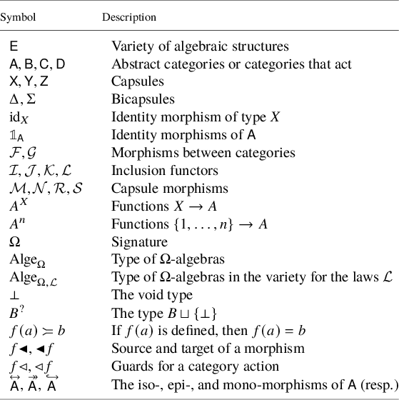
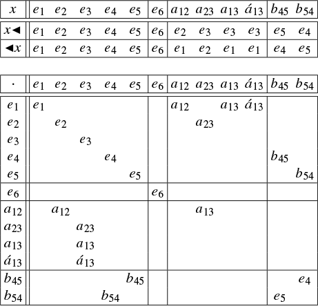

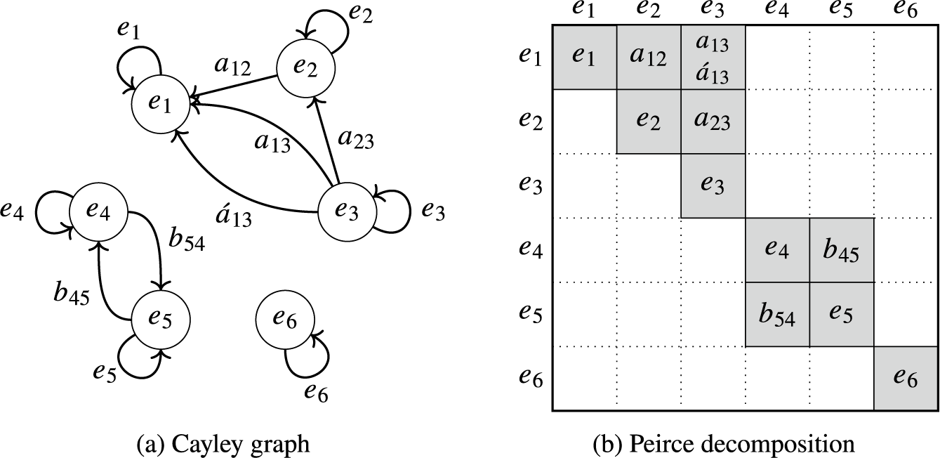

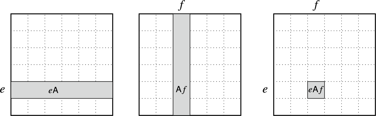

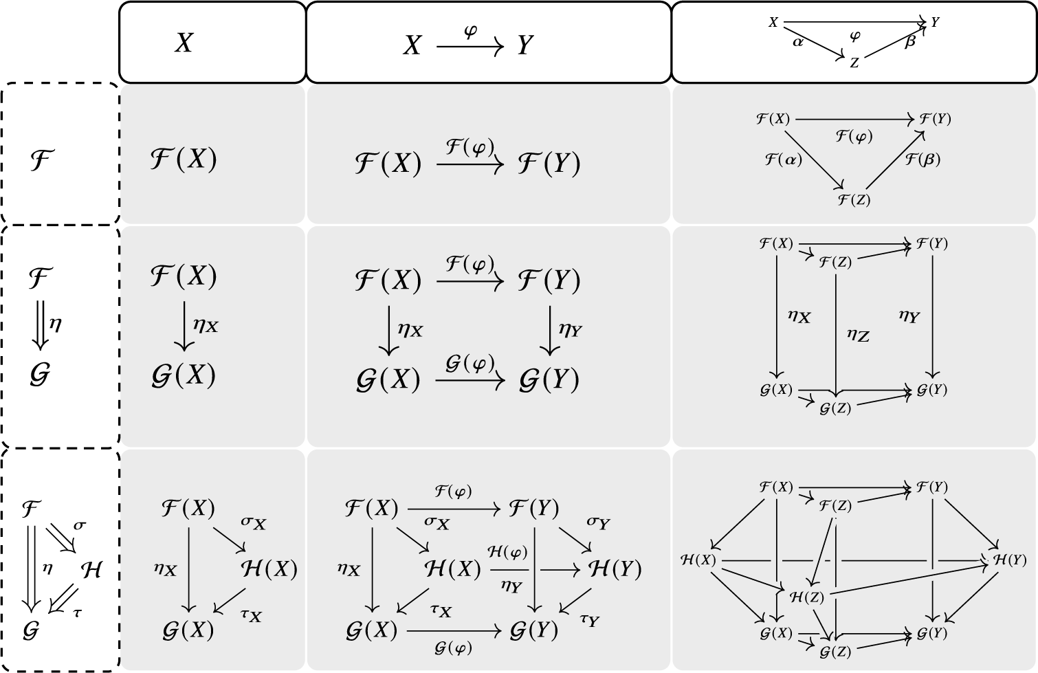


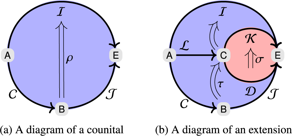
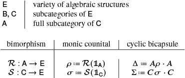
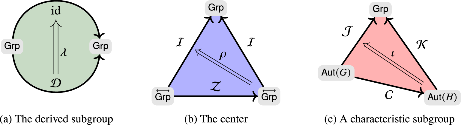
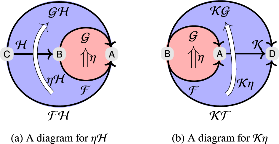
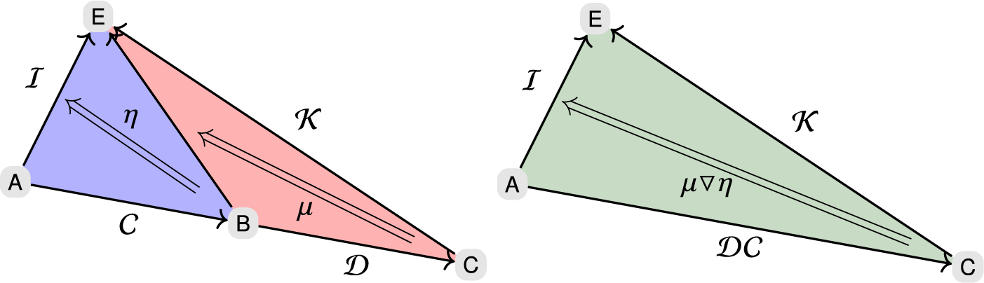

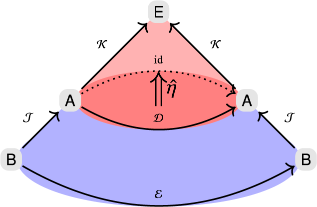
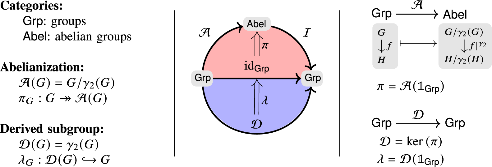
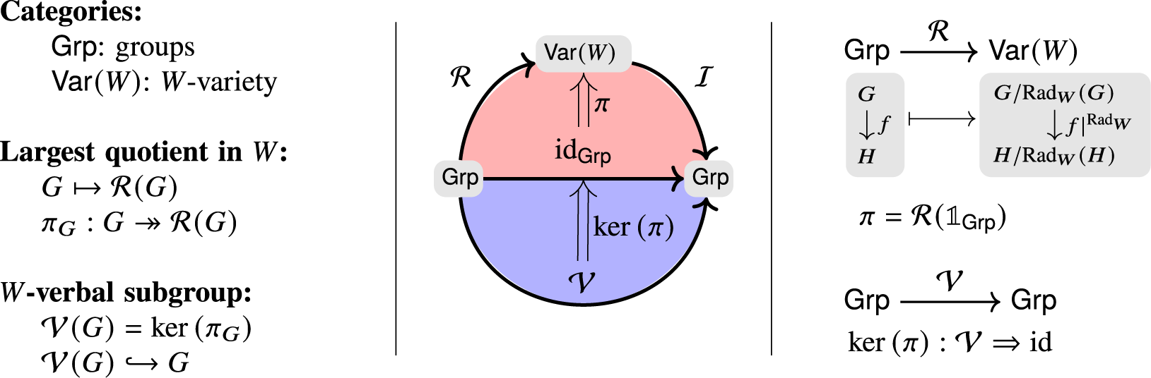
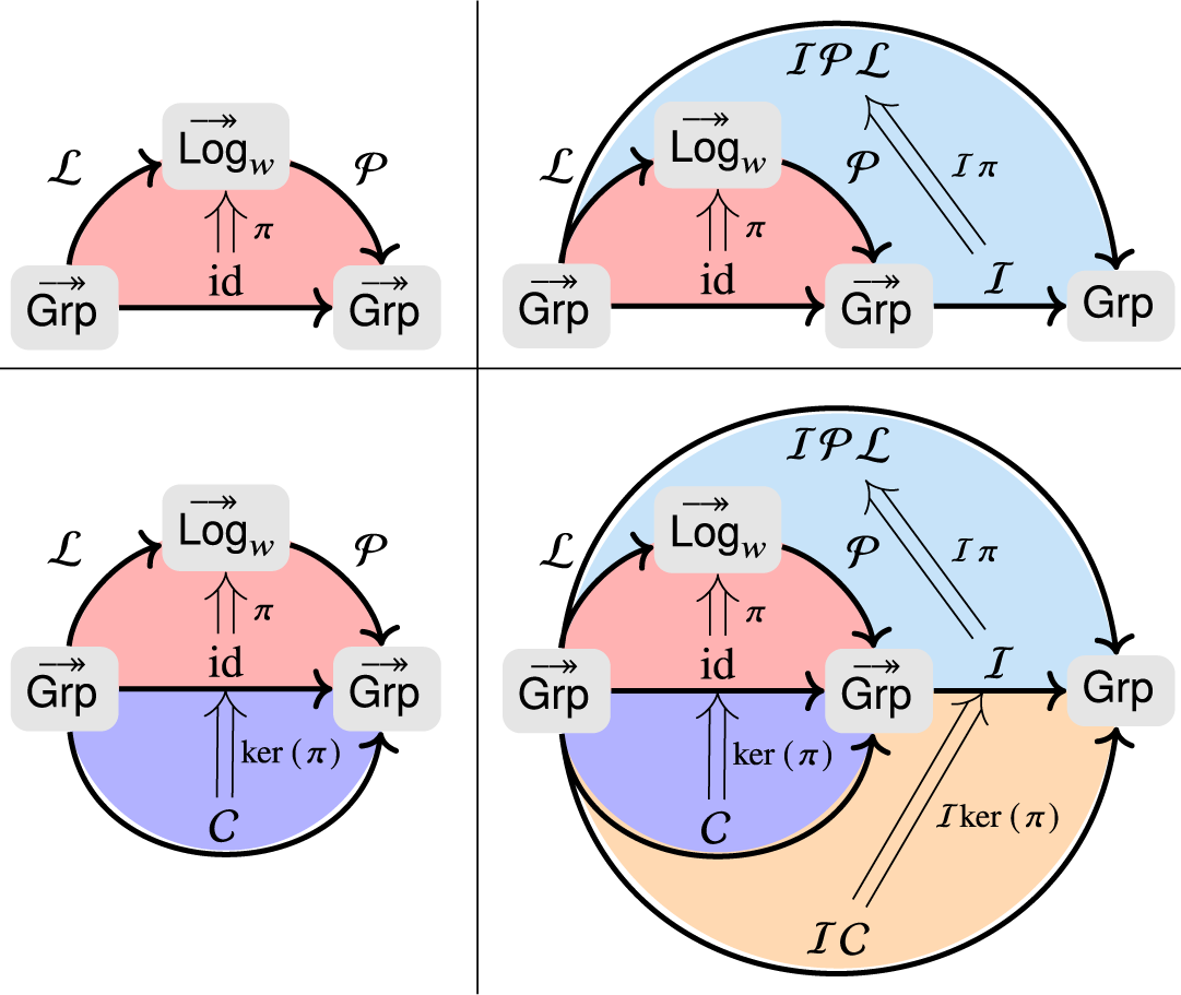

 Open access