


1. Introduction
There is a growing literature which questions the ability of traditional simple-sum money measures to provide a complete representation of liquidity in the economy. See, for example, Barnett (Reference Barnett1978, Reference Barnett1980, Reference Barnett and Barnett2016), Barnett and Chauvet (Reference Barnett and Chauvet2011), Hendrickson (Reference Hendrickson2014), Serletis and Gogas (Reference Serletis and Gogas2014), Belongia and Ireland (Reference Belongia and Ireland2014, Reference Belongia and Ireland2015, Reference Belongia and Ireland2016, Reference Belongia and Ireland2018, Reference Belongia and Ireland2021), Ellington (Reference Ellington2018), Jadidzadeh and Serletis (Reference Jadidzadeh and Serletis2019), Dai and Serletis (Reference Dai and Serletis2019), Serletis and Xu (Reference Serletis and Xu2020), and Dery and Serletis (Reference Dery and Serletis2021), among others. While statistical index number theory and microeconomic aggregation theory provide appealing alternatives to the simple-sum approach to monetary aggregation, they both rely on a number of assumptions about consumer preferences or the aggregator function of the representative economic agent. The estimation of the aggregator function usually requires that quantities and prices of monetary assets be observable and the aggregator function be weekly separable within tastes or technology of an economic agent’s complete aggregator function. See Barnett and Serletis (Reference Barnett and Serletis2008) for a discussion. In this paper, we partially relax these assumptions by allowing for unobserved assets in the aggregator function.
Starting in the early 1980s, in response to interest-rate volatility and improvements in computer and telecommunications technology, as well as banking deregulation, the U.S. banking sector went through a period of significant financial innovation, which led to the growth of the shadow banking system and transformed the entire financial system, considerably affecting the demand for money. Teles and Zhou (Reference Teles and Zhou2005) argue that these technological and regulatory changes justify a change in the way money is measured after 1980. Adrian and Ashcraft (Reference Adrian and Ashcraft2012) report that the share of traditional forms of financial intermediation declined from 100 percent in the mid-1940s to 40 percent by 2007 due to the development of the shadow banking system. As a result of this transformation, a part of the demand for transaction services has been driven away from traditional monetary instruments toward a large number of alternatives, such as, for example, digital currencies in recent years.
In this paper, we assume that some monetary assets are not observed directly and, therefore, their quantities and prices (user costs) cannot be used in the estimation of monetary demand systems and the construction of monetary aggregates (either statistical or functional). We then develop a model of monetary asset demand with unobserved assets. Although the quantities and user costs of the unobserved assets are latent, the unobserved demand for them affects the demand for observed monetary assets. Due to this reason, we are able to estimate a monetary asset demand system that includes unobserved assets. We propose a nonlinear filter and estimate the dynamics of user costs and quantities of unobserved monetary assets and then augment each of the CFS Divisia M1, Divisia M2, Divisia M3, and Divisia M4 monetary aggregates with unobserved monetary assets. We model an aggregator function and the demand for monetary assets using the normalized quadratic (NQ) locally flexible functional form introduced by Diewert and Wales (Reference Diewert and Wales1987). We use the likelihood inference to simultaneously estimate unobserved quantities, user costs, and the parameters of the monetary demand system induced by the aggregator function. Since the quantities of such assets are not observable, we exclude the corresponding equations from the estimating demand system. At the same time, the unobserved prices affect the demand for the observable assets via complementarity and substitutability relationships. We assume an autoregressive process for the unobserved prices and estimate the model in state-space form. Since the measurement equations are nonlinear we estimate the model using a particle filter.
One strand of the literature proposes redefining existing monetary aggregates by adding or removing observable assets in order to better capture liquidity services. Motley (Reference Motley1988) argues that M2 should be modified by adding institutional money-market mutual fund shares and excluding small time deposits. Poole (Reference Poole and Poole1994) introduces the term MZM (for “money zero maturity”) to describe such an aggregate composed entirely of zero-maturity assets. Teles and Zhou (Reference Teles and Zhou2005) advocate MZM as a superior empirical measure of money that restores the long-run relationship among money, prices, a measure of economic activity, and a nominal interest rate. More recently, Barnett and Su (Reference Barnett and Su2016) and Barnett et al. (Reference Barnett, Chauvet, Leiva-Leon and Su2024) extend the Divisia monetary aggregates to incorporate credit card transactions services and derive credit card-augmented Divisia monetary aggregates that jointly aggregate the services of money and credit cards. They provide evidence that the credit-augmented Divisia monetary aggregates have superior power in nowcasting nominal GDP compared to the original Divisia monetary aggregates and the official simple-sum monetary aggregates. An advantage of this approach is that it explicitly specifies what additional information is included in the new monetary aggregates. At the same time, the choice of a specific asset to include in the monetary aggregate is discretionary. As a result, multiple competing monetary aggregates augmented with alternative assets have already emerged. Moreover, assets that are potentially missing from conventional measures of money may change over time. Therefore, the continual inclusion of new assets (and potentially the exclusion of existing ones) would be required.
In contrast, our approach starts with an assumption that the money demand includes an unobserved asset without specifying the nature of the unobserved asset. A significant advantage of this approach is that it does not require arbitrary assumptions about what assets must be included in the measure of money. Also, the model captures the unobserved money demand which may include multiple assets whose composition changes over time. In our model, the unobserved asset enters the utility function symmetrically with the observed assets. Since the latent monetary asset affects demands for observable assets through substitutability and complementarity, we are able to recover its quantity and user cost using the demand for observable assets. In the estimation, we impose monotonicity and positivity constraints on quantities to ensure consistency with neoclassical demand theory. Therefore, the unobserved asset cannot enter the demand system in negative quantities or in a “ short position.” Importantly, if the data implied that the optimal quantity of the latent asset were zero, the estimated series would collapse toward zero. The fact that the estimated latent quantities are persistently positive is therefore an empirical outcome rather than a mechanical restriction. It is important to note that we make no additional assumptions about the total expenditure (budget) which also becomes unobserved with the inclusion of the unobserved asset. The total expenditure can be eliminated from the demand system even in some cases with nonhomothetic preferences.
It is to be noted that in a related paper, Barnett et al. (Reference Barnett, Chauvet and Tierney2009) recover common factors underlying monetary aggregate indices and compare the dynamics of the simple sum and Divisia monetary aggregates. They assume a linear relation between the latent factors and the monetary aggregates and use a modification of the Kalman filter which adopts regime switching. As Barnett et al. (Reference Barnett, Chauvet and Tierney2009, p. 408) put it, “the state-space time-series approach provides a highly promising direction for research into aggregation theory, index number theory, and economic policy.” However, Barnett et al. (Reference Barnett, Chauvet and Tierney2009) take a reduced-form approach and abstract from explicit derivation of the demand for monetary assets from consumer preferences. Thus, the nature of the common factors in monetary aggregates remains unclear.
Our findings suggest that these factors can stem from the demand for unobserved assets. The unobserved components in our structural model can capture the role of credit in monetary aggregation emphasized in Barnett and Su (Reference Barnett and Su2016) and Barnett et al. (Reference Barnett, Chauvet, Leiva-Leon and Su2024). It is especially evident from similar trend dynamics of the unobserved component in the M1 monetary aggregate and the credit cards balances. In addition, the demand for unobserved assets changes the relations between observed quantities demanded and their prices. This change can be interpreted as a structural break or Markov switching of the demand system parameters. For example, Isakin and Serletis (Reference Isakin and Serletis2019) and Xu and Serletis (Reference Xu and Serletis2022) document significant shifts in the parameters of the demands for monetary assets and estimate their models with Markov switching parameters.
We follow Belongia and Ireland (Reference Belongia and Ireland2021) and estimate a five-equation structural VAR model of monetary business cycle with the monetary aggregates. We report impulse response functions of the inflation rate and the output gap to shocks to monetary policy, money demand, and monetary system. The models with the original Divisia M1 and Divisia M2 aggregates produce an output puzzle, i.e. an increase in the output gap in response to a positive shock to the interest rate. We observe that models with the augmented Divisia monetary aggregates produce results consistent with a priori expectations about the effects of monetary policy on output and inflation. Finally, we analyze the relationship between real money, income and the nominal interest rate, with a unitary income elasticity. As documented by Lucas (Reference Lucas1988), the real balances demonstrated a strong negative response to the nominal interest rate until the mid-1980s but the relationship breaks afterwards. This suggests that the demand for money might not be a stable relationship at least with M1. We demonstrate that with our new monetary aggregates money demand has no conspicuous structural break and fits the data well. We also show that money-income ratios and corresponding user costs have significant negative relations for our augmented monetary aggregates at all levels of aggregation while this relation is insignificant for the original Divisia M3 and Divisia M4 aggregates.
The rest of the paper is organized as follows. Sections 2 and 3 briefly sketch related neoclassical demand theory, present the NQ expenditure function, derive the associated system of budget share equations, and discuss the Diewert and Wales (Reference Diewert and Wales1988) method of imposing global concavity with the objective of achieving theoretical regularity. Section 4 presents the unobserved components NQ demand system and section 5 discusses econometric issues and the particle filter. Section 6 discusses the data and presents the empirical results. The final section concludes regarding the implications of our research for monetary theory, the conduct of monetary policy, and business cycle analysis.
2. The model
Let’s consider an economy with identical households whose direct utility function is weakly separable (a direct tree) as follows
 \begin{align} U=u(\boldsymbol{{c}},\ell ,f(\boldsymbol{{x}})) \end{align}
where
 $\boldsymbol{{c}}$
is a vector of the services of consumption goods,
$\boldsymbol{{c}}$
is a vector of the services of consumption goods,
 $\ell$
is leisure time,
$\ell$
is leisure time,
 $\boldsymbol{{x}}$
is a vector of the services of monetary assets (assumed to be proportional to the stocks), and
$\boldsymbol{{x}}$
is a vector of the services of monetary assets (assumed to be proportional to the stocks), and
 $f(\boldsymbol{{x}})$
is a monetary services aggregator function. In accordance with the assignment of monetary assets to monetary aggregates by the Center for Financial Stability (CFS), we assume that the aggregator function,
$f(\boldsymbol{{x}})$
is a monetary services aggregator function. In accordance with the assignment of monetary assets to monetary aggregates by the Center for Financial Stability (CFS), we assume that the aggregator function,
 $f(\boldsymbol{{x}})$
, has the homothetically strongly recursive separable form
$f(\boldsymbol{{x}})$
, has the homothetically strongly recursive separable form
 \begin{equation} f(\boldsymbol{{x}})=f_{4}(\boldsymbol{{x}}_{4}\text{, }f_{3}(\boldsymbol{{x}}_{3},f_{2}(\boldsymbol{{x}}_{2},f_{1}(\boldsymbol{{x}}_{1})))) \end{equation}
where the components of
 $\boldsymbol{{x}}$
 $_{1}$
are those that are included in the CFS M1 monetary aggregate (assets
$_{1}$
are those that are included in the CFS M1 monetary aggregate (assets
 $x_{1}$
and
$x_{1}$
and
 $x_{2}$
in Table 1), the components of
$x_{2}$
in Table 1), the components of
 $\boldsymbol{{x}}$
 $_{2}$
are those of the CFS M2 aggregate net of
$_{2}$
are those of the CFS M2 aggregate net of
 $\boldsymbol{{x}}$
 $_{1}$
(that is, assets
$_{1}$
(that is, assets
 $x_{3}$
and
$x_{3}$
and
 $x_{4}$
in Table 1), the components of
$x_{4}$
in Table 1), the components of
 $\boldsymbol{{x}}$
 $_{3}$
are those of the CFS M3 aggregate net of
$_{3}$
are those of the CFS M3 aggregate net of
 $\boldsymbol{{x}}$
 $_{1}$
and
$_{1}$
and
 $\boldsymbol{{x}}$
 $_{2}$
(that is, assets
$_{2}$
(that is, assets
 $x_{5}$
,
$x_{5}$
,
 $x_{6}$
, and
$x_{6}$
, and
 $x_{7}$
in Table 1), and the components of
$x_{7}$
in Table 1), and the components of
 $\boldsymbol{{x}}$
 $_{4}$
are assets
$_{4}$
are assets
 $x_{8}$
and
$x_{8}$
and
 $x_{9}$
in Table 1. The (monotonically increasing and strictly quasi-concave) aggregator functions,
$x_{9}$
in Table 1. The (monotonically increasing and strictly quasi-concave) aggregator functions,
 $f_{i}$
 $\left ( i=1,2,3,4\right )$
, in (2) are the CFS functional monetary aggregates
$\left ( i=1,2,3,4\right )$
, in (2) are the CFS functional monetary aggregates
 $Q_{1}$
,
$Q_{1}$
,
 $Q_{2}$
,
$Q_{2}$
,
 $Q_{3}$
, and
$Q_{3}$
, and
 $Q_{4}$
, respectively. In particular, if
$Q_{4}$
, respectively. In particular, if
 $Q_{1}$
is the functional monetary aggregate for the components of M1,
$Q_{1}$
is the functional monetary aggregate for the components of M1,
 $Q_{2}$
for M2,
$Q_{2}$
for M2,
 $Q_{3}$
for M3, and
$Q_{3}$
for M3, and
 $Q_{4}$
for M4, then it follows that
$Q_{4}$
for M4, then it follows that
 \begin{align} Q_{1}& =f_{1}(\boldsymbol{{x}}_{1})\text{;} \end{align}
 \begin{align} Q_{2}& =f_{2}\left [ \boldsymbol{{x}}_{2},f_{1}(\boldsymbol{{x}}_{1})\right ] =f_{2}\left ( \boldsymbol{{x}}_{2},Q_{1}\right ) \text{;} \end{align}
 \begin{align} Q_{3}& =f_{3}\left \{ \boldsymbol{{x}}_{3},f_{2}\left [ \boldsymbol{{x}}_{2},f_{1}(\boldsymbol{{x}}_{1})\right ] \right \} =f_{3}(\boldsymbol{{x}}_{3},Q_{2})\text{;}\quad \text{and} \end{align}
 \begin{align} Q_{4}& =f_{4}\left ( \boldsymbol{{x}}_{4},f_{3}\left \{ \boldsymbol{{x}}_{3},f_{2}\left [ \boldsymbol{{x}}_{2},f_{1}(\boldsymbol{{x}}_{1})\right ] \right \} \right ) =f_{4}(\boldsymbol{{x}}_{4},Q_{3})\text{.} \end{align}
Each aggregator function,
 $f_{i}$
 $\left ( i=1,2,3,4\right )$
, is thought of as a category utility function as well as a subaggregate measure of monetary services. For purposes of investigating the demand for Divisia money, the monetary aggregates,
$\left ( i=1,2,3,4\right )$
, is thought of as a category utility function as well as a subaggregate measure of monetary services. For purposes of investigating the demand for Divisia money, the monetary aggregates,
 $Q_{1}$
,
$Q_{1}$
,
 $Q_{2}$
,
$Q_{2}$
,
 $Q_{3}$
, and
$Q_{3}$
, and
 $Q_{4}$
in equations (3)–(6) would be thought of as Divisia quantity indices, which correspond to Divisia price indices,
$Q_{4}$
in equations (3)–(6) would be thought of as Divisia quantity indices, which correspond to Divisia price indices,
 $P_{1}$
,
$P_{1}$
,
 $P_{2}$
,
$P_{2}$
,
 $P_{3}$
, and
$P_{3}$
, and
 $P_{4}$
, respectively.
$P_{4}$
, respectively.
The components of monetary aggregates

Note: Asset
 $x_{1}$
(Cash assets) includes currency, traveler’s checks, and demand deposits. Asset
$x_{1}$
(Cash assets) includes currency, traveler’s checks, and demand deposits. Asset
 $x_{2}$
(Other liquid deposits) includes OCDs, saving deposits, and MMDAs at commercial banks and thrift institutions. Asset
$x_{2}$
(Other liquid deposits) includes OCDs, saving deposits, and MMDAs at commercial banks and thrift institutions. Asset
 $x_{4}$
(Small time deposits) includes small-denomination and small time deposits at commercial banks and thrift institutions.
$x_{4}$
(Small time deposits) includes small-denomination and small time deposits at commercial banks and thrift institutions.
In order to focus on the details of the demand for money at different levels of monetary aggregation, we follow Serletis (Reference Serletis1987) and assume a multistage decentralization procedure according to which the representative agent derives the demand for monetary services at different levels of aggregation from a recursively decentralized optimization problem. Although the consumer is viewed as making the decentralization decisions from the top of the tree down, we will elaborate on the multistage decentralization properties of decision (1)—and we will later estimate conditional money demand models at successive levels of aggregation—recursively, from the bottom up.
The first-stage decision is to select
 $\boldsymbol{{x}}$
 $_{1}$
to solve
$_{1}$
to solve
 \begin{equation*} \max _{\left (\boldsymbol{{x}}_{1}\right )}f_{1}(\boldsymbol{{x}}_{1})\quad \text{subject to } \boldsymbol{{p}}_{1}\boldsymbol{{x}}_{1}=P_{1} Q_{1} \end{equation*}
where
 $\boldsymbol{{p}}_{1}$
is the vector of user costs corresponding to
$\boldsymbol{{p}}_{1}$
is the vector of user costs corresponding to
 $\boldsymbol{{x}}$
 $_{1}$
. The second, third, and fourth stages of the multistage decision are as follows
$_{1}$
. The second, third, and fourth stages of the multistage decision are as follows
 \begin{equation*} \max _{(\boldsymbol{{x}}_{i},Q_{i-1})}f_{i}\left (\boldsymbol{{x}}_{i},Q_{i-1}\right )\quad \text{subject to } \boldsymbol{{p}}_{i}\boldsymbol{{x}}_{i}+P_{i-1}Q_{i-1}=P_{i}Q_{i}\text{, }i=2,3,4 \end{equation*}
where
 $\boldsymbol{{p}}_{i}$
is the vector of user costs corresponding to
$\boldsymbol{{p}}_{i}$
is the vector of user costs corresponding to
 $\boldsymbol{{x}}_{i}$
,
$\boldsymbol{{x}}_{i}$
,
 $P_{i}$
is a Divisia price index corresponding to the Divisia quantity aggregate
$P_{i}$
is a Divisia price index corresponding to the Divisia quantity aggregate
 $Q_{i}$
,
$Q_{i}$
,
 $i=2,3,4$
.
$i=2,3,4$
.
At the most aggregate level, the problem is
 \begin{equation*} \max _{({ \boldsymbol{{c}} },\ell ,Q_{4})}u\left ({ \boldsymbol{{c}} },\ell ,Q_{4}\right )\quad \text{subject to } \boldsymbol{\phi } \boldsymbol{{c}} +w\ell +P_{4}Q_{4}=y \end{equation*}
where
 $\boldsymbol{\phi }$
is the vector of prices of consumption goods,
$\boldsymbol{\phi }$
is the vector of prices of consumption goods,
 $\boldsymbol{{c}}$
,
$\boldsymbol{{c}}$
,
 $w$
is the opportunity cost of leisure,
$w$
is the opportunity cost of leisure,
 $\ell$
,
$\ell$
,
 $P_{4}$
is a Divisia price index corresponding to the Divisia quantity aggregate
$P_{4}$
is a Divisia price index corresponding to the Divisia quantity aggregate
 $Q_{4}$
, and
$Q_{4}$
, and
 $y$
is total income.
$y$
is total income.
3. The NQ expenditure function
We use the NQ expenditure function introduced by Diewert and Wales (Reference Diewert and Wales1988) to estimate the demand equations at each stage of the multistage decision. The NQ expenditure function is locally flexible, capable of approximating an arbitrary twice continuously differentiable function to the second order at an arbitrary point in the domain. Moreover, curvature can be imposed globally without losing the flexibility property. We impose several restrictions on the NQ parameters to satisfy the regularity conditions and produce inference consistent with neoclassical microeconomic theory.
In the general case with
 $n$
goods (
$n$
goods (
 $x_{1},\ldots ,x_{n}$
), for a given level of utility
$x_{1},\ldots ,x_{n}$
), for a given level of utility
 $u$
and the vector of prices (user costs)
$u$
and the vector of prices (user costs)
 $\boldsymbol{{p}}$
, the NQ expenditure function is
$\boldsymbol{{p}}$
, the NQ expenditure function is
 \begin{equation} C\left ({ \boldsymbol{{p}} },u\right )={ \boldsymbol{{d}} }^{\prime }{ \boldsymbol{{p}} }+\left ({ \boldsymbol{{b}} }^{\prime }{ \boldsymbol{{p}} }+\frac {{ \boldsymbol{{p}} }^{\prime }{ \boldsymbol{{C}} \boldsymbol{{p}} }}{2{ \boldsymbol{\alpha } }^{\prime }{ \boldsymbol{{p}} }}\right )u \end{equation}
where
 $\boldsymbol{{d}}=[d_{1},d_{2},\ldots ,d_{n}]^{\prime }, \boldsymbol{{b}}=[b_{1},\ldots ,b_{n}]^{\prime }$
, and the
$\boldsymbol{{d}}=[d_{1},d_{2},\ldots ,d_{n}]^{\prime }, \boldsymbol{{b}}=[b_{1},\ldots ,b_{n}]^{\prime }$
, and the
 $n\times n$
matrix
$n\times n$
matrix
 $\boldsymbol{{C}}\ =[c_{ij}]$
are the unknown parameters to be estimated. The vector of parameters
$\boldsymbol{{C}}\ =[c_{ij}]$
are the unknown parameters to be estimated. The vector of parameters
 $\boldsymbol{\alpha }^{\prime }=[\alpha _{1},\ldots ,\alpha _{n}]$
is predetermined and satisfies
$\boldsymbol{\alpha }^{\prime }=[\alpha _{1},\ldots ,\alpha _{n}]$
is predetermined and satisfies
 $\boldsymbol{\alpha }\gt \boldsymbol{0}_{n}$
. We follow Diewert and Wales (Reference Diewert and Wales1988) and impose the following restrictions on the parameters. The quadratic form matrix
$\boldsymbol{\alpha }\gt \boldsymbol{0}_{n}$
. We follow Diewert and Wales (Reference Diewert and Wales1988) and impose the following restrictions on the parameters. The quadratic form matrix
 $\boldsymbol{{C}}$
is symmetric, i.e.
$\boldsymbol{{C}}$
is symmetric, i.e.
 $c_{kl}=c_{lk}$
for
$c_{kl}=c_{lk}$
for
 $k,l=1,\ldots ,n$
. Further, at some reference price vector
$k,l=1,\ldots ,n$
. Further, at some reference price vector
 $\boldsymbol{{p}}^{\ast }\gg \boldsymbol{0}$
 \begin{align} { \boldsymbol{\alpha } }^{\prime }{ \boldsymbol{{p}} }^{\ast } & ={ \boldsymbol{1} } \notag \\ { \boldsymbol{{d}} }^{\prime }{ \boldsymbol{{p}} }^{\ast } & ={ \boldsymbol{0} } \notag \\ { \boldsymbol{{b}} }^{\prime }{ \boldsymbol{{p}} }^{\ast } & ={ \boldsymbol{1} } \end{align}
 \begin{align} { \boldsymbol{{C}} \boldsymbol{{p}} }^{\ast } & ={ \boldsymbol{0} }_{n}\text{,}\quad { \boldsymbol{{C}} }={ \boldsymbol{{C}} }^{\prime }\text{.} \end{align}
Normalizations (8) and (9) are required for cardinalization of utility—see Diewert and Wales (Reference Diewert and Wales1988) for more details. For example, if
 $\boldsymbol{{p}}^{\ast }=\boldsymbol{1}$
then the elements of the last row and column of
$\boldsymbol{{p}}^{\ast }=\boldsymbol{1}$
then the elements of the last row and column of
 $\boldsymbol{{C}}$
can be expressed using (9).
$\boldsymbol{{C}}$
can be expressed using (9).
Shephard’s (Reference Shephard1953) lemma applies and the NQ Marshallian demand system is given by
 \begin{equation} \boldsymbol{{x}}({ \boldsymbol{{p}} },y)={ \boldsymbol{{d}} }+\frac {{ \boldsymbol{{b}} }\left ({ \boldsymbol{\alpha } }^{\prime }{ \boldsymbol{{p}} }\right )^{2}+{ \boldsymbol{{C}} \boldsymbol{{p}} }\left ({ \boldsymbol{\alpha } }^{\prime }{ \boldsymbol{{p}} }\right )-0.5{ \boldsymbol{\alpha } \boldsymbol{{p}} }^{\prime }{ \boldsymbol{{C}} \boldsymbol{{p}} }}{\left ({ \boldsymbol{\alpha } }^{\prime }{ \boldsymbol{{p}} }\right ){ \boldsymbol{{b}} }^{\prime }{ \boldsymbol{{p}} }+0.5{ \boldsymbol{{p}} }^{\prime }{ \boldsymbol{{C}} \boldsymbol{{p}} }}\times \frac {y-{ \boldsymbol{{d}} }^{\prime }{ \boldsymbol{{p}} }}{{ \boldsymbol{\alpha } }^{\prime }{ \boldsymbol{{p}} }} \end{equation}
where
 $y=\boldsymbol{{p}}^{\prime }\boldsymbol{{x}}$
is the total expenditure.
$y=\boldsymbol{{p}}^{\prime }\boldsymbol{{x}}$
is the total expenditure.
The expenditure function (7) is concave if and only if
 $\boldsymbol{{C}}$
is negative semidefinite. We follow Diewert and Wales (Reference Diewert and Wales1988) to ensure concavity with respect to prices. Since the last row and column of
$\boldsymbol{{C}}$
is negative semidefinite. We follow Diewert and Wales (Reference Diewert and Wales1988) to ensure concavity with respect to prices. Since the last row and column of
 $\boldsymbol{{C}}$
can be expressed using (9), we let
$\boldsymbol{{C}}$
can be expressed using (9), we let
 $\widetilde {{ \boldsymbol{{C}} }}$
denote the
$\widetilde {{ \boldsymbol{{C}} }}$
denote the
 $(n-1)\times (n-1)$
matrix of “free parameters. Then we impose
$(n-1)\times (n-1)$
matrix of “free parameters. Then we impose
 $\widetilde {{ \boldsymbol{{C}} }}=-\boldsymbol{{G}}\boldsymbol{{G}}^{\prime }$
, where
$\widetilde {{ \boldsymbol{{C}} }}=-\boldsymbol{{G}}\boldsymbol{{G}}^{\prime }$
, where
 $\boldsymbol{{G}}=[g_{ij}]$
is an
$\boldsymbol{{G}}=[g_{ij}]$
is an
 $(n-1)\times (n-1)$
lower triangular matrix. With all restrictions imposed, the demand system (10) has a total of
$(n-1)\times (n-1)$
lower triangular matrix. With all restrictions imposed, the demand system (10) has a total of
 $ 2n-2+0.5n(n-1)$
parameters. Even if all quantities demanded are observable, an estimation of the system with an additive error term should use
$ 2n-2+0.5n(n-1)$
parameters. Even if all quantities demanded are observable, an estimation of the system with an additive error term should use
 $n-1$
equations as the covariance matrix of the error terms of the whole system is singular—see Diewert and Wales (Reference Diewert and Wales1988).
$n-1$
equations as the covariance matrix of the error terms of the whole system is singular—see Diewert and Wales (Reference Diewert and Wales1988).
4. The NQ system with unobserved assets
We assume that in each monetary aggregate, M1, M2, M3, and M4, one monetary asset is not observed.Footnote
1
In what follows, for expositional simplicity, we omit the level of aggregation index. Without loss of generality, we assume that the last,
 $n$
th, asset is not observed, i.e., the last price
$n$
th, asset is not observed, i.e., the last price
 $p_{nt}$
in vector
$p_{nt}$
in vector
 $\boldsymbol{{p}}_{t}$
and the last quantity
$\boldsymbol{{p}}_{t}$
and the last quantity
 $x_{nt}$
in vector
$x_{nt}$
in vector
 $\boldsymbol{{x}}_{t}$
are not observed. While that price is unobserved, it affects demands for the observed assets due to complementarity or substitutability across the assets.
$\boldsymbol{{x}}_{t}$
are not observed. While that price is unobserved, it affects demands for the observed assets due to complementarity or substitutability across the assets.
Further, we assume that the logarithm of
 $p_{nt}$
follows a random walk processes
$p_{nt}$
follows a random walk processes
 \begin{equation} \ln p_{nt} = \ln p_{n,t-1}+v_{t} \end{equation}
where the innovation shock (error)
 $v_{t}\sim N(0,\sigma _{v}^{2})$
with variance
$v_{t}\sim N(0,\sigma _{v}^{2})$
with variance
 $\sigma _{v}^{2}$
. As we discuss in Section 6, all price series in our sample suggest unit roots. We assume that the prices of observed assets are observed exactly. Since there are no adjustment costs, the dynamics of the prices have no effect on the optimal decision of the representative consumer in each period. Thus, the demand for monetary assets in each period is given by the NQ demand system (10). Since the quantities of some assets are not observable, the measurement equation includes quantities of observed assets only.
$\sigma _{v}^{2}$
. As we discuss in Section 6, all price series in our sample suggest unit roots. We assume that the prices of observed assets are observed exactly. Since there are no adjustment costs, the dynamics of the prices have no effect on the optimal decision of the representative consumer in each period. Thus, the demand for monetary assets in each period is given by the NQ demand system (10). Since the quantities of some assets are not observable, the measurement equation includes quantities of observed assets only.
The right-hand side of (10) cannot be evaluated because it has entries of unobserved total expenditure
 $y_{t}$
in period
$y_{t}$
in period
 $t$
. To eliminate
$t$
. To eliminate
 $ y_{t}$
from the demand equations, we express
$ y_{t}$
from the demand equations, we express
 $\left ( y_{t}-{ \boldsymbol{{d}} }_{t}^{\prime }{ \boldsymbol{{p}} }_{t}\right ) \left ( { \boldsymbol{\alpha } }^{\prime }{ \boldsymbol{{p}} }_{t}\right ) ^{-1}$
from the first equation and plug it into the other equations. Though we assume nonhomothetic preferences, the demand equations depend on total expenditure in a simple way that allows us to eliminate the total expenditure from the system. It is an important step of our model that allows us to estimate the system without making additional assumptions about the unobserved total expenditure. We assume an additive measurement error and write the rearranged system in scalar form
$\left ( y_{t}-{ \boldsymbol{{d}} }_{t}^{\prime }{ \boldsymbol{{p}} }_{t}\right ) \left ( { \boldsymbol{\alpha } }^{\prime }{ \boldsymbol{{p}} }_{t}\right ) ^{-1}$
from the first equation and plug it into the other equations. Though we assume nonhomothetic preferences, the demand equations depend on total expenditure in a simple way that allows us to eliminate the total expenditure from the system. It is an important step of our model that allows us to estimate the system without making additional assumptions about the unobserved total expenditure. We assume an additive measurement error and write the rearranged system in scalar form
 \begin{equation} x_{it}=d_{i}+\frac {\phi ^{2}b_{i}+\phi \sum _{j}C_{ij}p_{jt}-0.5\alpha _{i}\sum _{j}\sum _{k}C_{jk}p_{kt}p_{jt}}{\phi ^{2}b_{1}+\phi \sum _{j}C_{1j}p_{jt}-0.5\alpha _{1}\sum _{j}\sum _{k}C_{jk}p_{kt}p_{jt}}\left ( x_{1t}-d_{1}\right ) +\varepsilon _{it} \end{equation}
for
 $i=2,\ldots ,n$
, where
$i=2,\ldots ,n$
, where
 $\phi =\sum _{j}\alpha _{j}p_{jt}$
and
$\phi =\sum _{j}\alpha _{j}p_{jt}$
and
 $\boldsymbol{\varepsilon }_{t}=\left ( \varepsilon _{2t},\ldots ,\varepsilon _{nt}\right ) \sim N(\boldsymbol{0},\mathbf{\Sigma }_{{ \boldsymbol{\varepsilon }}})$
. The resulting system contains
$\boldsymbol{\varepsilon }_{t}=\left ( \varepsilon _{2t},\ldots ,\varepsilon _{nt}\right ) \sim N(\boldsymbol{0},\mathbf{\Sigma }_{{ \boldsymbol{\varepsilon }}})$
. The resulting system contains
 $n-1$
equations but the last equation cannot be used in estimation because it has the unobserved quantity in the left hand side. All equations contain unobserved prices which should be estimated together with unknown parameters of the NQ expenditure function. To reduce the number of estimated parameters, we assume that the covariance matrix
$n-1$
equations but the last equation cannot be used in estimation because it has the unobserved quantity in the left hand side. All equations contain unobserved prices which should be estimated together with unknown parameters of the NQ expenditure function. To reduce the number of estimated parameters, we assume that the covariance matrix
 $\mathbf{\Sigma }_{{ \boldsymbol{\varepsilon } }}$
is diagonal. Then the total number of parameters becomes
$\mathbf{\Sigma }_{{ \boldsymbol{\varepsilon } }}$
is diagonal. Then the total number of parameters becomes
 $ 2n-2+0.5n(n-1)+n+1$
where the last two terms correspond to the variances of the errors in equations (11) and (12). The system can be estimated using the maximum likelihood method, the generalized method of moments or Bayesian methods.
$ 2n-2+0.5n(n-1)+n+1$
where the last two terms correspond to the variances of the errors in equations (11) and (12). The system can be estimated using the maximum likelihood method, the generalized method of moments or Bayesian methods.
The model in state-space form is given by the measurement equation (12) and the transition equation (11). Rothenberg (Reference Rothenberg1971) shows that a model is locally identified at a point if and only if the information matrix is nonsingular in the neighborhood around this point. We demonstrate that model parameters are (locally) identified using a Monte Carlo experiment. In Section 6.2 we report the estimates of model parameters with robust standard error proposed by White (Reference White1982) which use the inverse of the information matrix. We would like to note that since system (12) is nonlinear in unobserved prices we do not have to use a normalization of parameters or the unobserved series (e.g., as in Barnett et al. (Reference Barnett, Chauvet and Tierney2009)) to achieve identifiability.
In general, the NQ approximation can violate the regularity properties of the utility function. The replacement
 $\widetilde {{ \boldsymbol{{C}} }}=-\boldsymbol{{G}}\boldsymbol{{G}}^{\prime }$
discussed above ensures the concavity of the utility function. However, the monotonicity property, i.e. the nonincreasing relation between quantities and corresponding prices, can fail in some regions. For discussion see Barnett (Reference Barnett2002). In practice, monotonicity usually holds in the sample region if the quality of fit is satisfactory. This is because an estimated demand system is derived by applying Shephard’s lemma which equates first order derivatives of the utility function to positive demands. Similarly, the positivity of fitted demand quantities is typically satisfied if the fit is good. However, since an estimated demand system imposes no restrictions on the monotonicity and positivity of unobserved quantities, it is likely that these properties will be violated in some regions for the unobserved quantities. We impose monotonicity and positivity in the particle filter as discussed in Appendix A.Footnote
2
At the same time, if concavity is imposed as discussed, the concavity of the utility function will be satisfied globally with respect to all quantities including unobserved quantities. It should be noted that since we impose monotonicity globally along with curvature, the flexibility in the sense of Diewert and Wales (Reference Diewert and Wales1987) of the estimated function form cannot be guaranteed.
$\widetilde {{ \boldsymbol{{C}} }}=-\boldsymbol{{G}}\boldsymbol{{G}}^{\prime }$
discussed above ensures the concavity of the utility function. However, the monotonicity property, i.e. the nonincreasing relation between quantities and corresponding prices, can fail in some regions. For discussion see Barnett (Reference Barnett2002). In practice, monotonicity usually holds in the sample region if the quality of fit is satisfactory. This is because an estimated demand system is derived by applying Shephard’s lemma which equates first order derivatives of the utility function to positive demands. Similarly, the positivity of fitted demand quantities is typically satisfied if the fit is good. However, since an estimated demand system imposes no restrictions on the monotonicity and positivity of unobserved quantities, it is likely that these properties will be violated in some regions for the unobserved quantities. We impose monotonicity and positivity in the particle filter as discussed in Appendix A.Footnote
2
At the same time, if concavity is imposed as discussed, the concavity of the utility function will be satisfied globally with respect to all quantities including unobserved quantities. It should be noted that since we impose monotonicity globally along with curvature, the flexibility in the sense of Diewert and Wales (Reference Diewert and Wales1987) of the estimated function form cannot be guaranteed.
5. Estimation
5.1 The estimation method
The model in the state-space form is given by the transition equation (11) and the observation equation (12). We let
 $\boldsymbol{\vartheta }$
denote the vector of stacked model parameters, namely, first
$\boldsymbol{\vartheta }$
denote the vector of stacked model parameters, namely, first
 $n-1$
elements of
$n-1$
elements of
 $\boldsymbol{{d}}$
, first
$\boldsymbol{{d}}$
, first
 $n-1$
elements of
$n-1$
elements of
 $\boldsymbol{{b}}$
,
$\boldsymbol{{b}}$
,
 $0.5n(n-1)$
nonzero elements of lower triangular matrix
$0.5n(n-1)$
nonzero elements of lower triangular matrix
 $\boldsymbol{{C}}$
,
$\boldsymbol{{C}}$
,
 $n$
diagonal elements of
$n$
diagonal elements of
 $\mathbf{\Sigma }_{{\boldsymbol{\varepsilon }}}$
, variance
$\mathbf{\Sigma }_{{\boldsymbol{\varepsilon }}}$
, variance
 $\sigma _{v}^{2}$
of the error term in the transition equation (11), and the initial value
$\sigma _{v}^{2}$
of the error term in the transition equation (11), and the initial value
 $z_{0}$
of the unobserved user cost. We also denote
$z_{0}$
of the unobserved user cost. We also denote
 $\boldsymbol{{q}}_{t}=\{\hat {\boldsymbol{{p}}}_{t},\hat {\boldsymbol{{x}}}_{t}\}$
, where
$\boldsymbol{{q}}_{t}=\{\hat {\boldsymbol{{p}}}_{t},\hat {\boldsymbol{{x}}}_{t}\}$
, where
 $\hat {\boldsymbol{{p}}}_{t}=(p_{1t},\ldots ,p_{n-1,t})^{\prime }$
is the vector of all observed prices and
$\hat {\boldsymbol{{p}}}_{t}=(p_{1t},\ldots ,p_{n-1,t})^{\prime }$
is the vector of all observed prices and
 $\hat {\boldsymbol{{x}}}_{t}=(x_{1t},\ldots ,x_{n-1,t})^{\prime }$
is the vector of all observed quantities. We use
$\hat {\boldsymbol{{x}}}_{t}=(x_{1t},\ldots ,x_{n-1,t})^{\prime }$
is the vector of all observed quantities. We use
 $\boldsymbol{{q}}_{1:T}$
and
$\boldsymbol{{q}}_{1:T}$
and
 $p_{n,1:T}$
to denote the whole path of
$p_{n,1:T}$
to denote the whole path of
 $\boldsymbol{{q}}_t$
and unobserved price
$\boldsymbol{{q}}_t$
and unobserved price
 $p_{nt}$
, respectively, over
$p_{nt}$
, respectively, over
 $t=1,\ldots ,T$
.
$t=1,\ldots ,T$
.
We estimate the model parameters and the unobserved price using the maximum likelihood method. We factorize the joint distribution of the parameters and the latent state variable conditional on the observed prices and quantities as follows:
 \begin{equation} \psi ({ \boldsymbol{\vartheta } },p_{n,1:T}|{ \boldsymbol{{q}} }_{1:T})=\psi (p_{n,1:T}|{ \boldsymbol{\vartheta } },{ \boldsymbol{{q}} }_{1:T})\psi ({ \boldsymbol{\vartheta } }|{ \boldsymbol{{q}} }_{1:T})\text{.} \end{equation}
Using decomposition (13), we estimate the model by maximum likelihood. For any given parameter vector, we filter the unobserved user costs (i.e., the latent state variable) using a particle filter and evaluate the associated likelihood of the observed data. We then maximize this likelihood with respect to the parameter vector.
Specifically, we construct a particle filter based on the bootstrap filter originally proposed in Gordon et al. (Reference Gordon, Salmond and Smith1993). In addition to producing filtered estimates of the latent state variable, the particle filter provides an approximation to the likelihood of the model conditional on the parameter values. The particle filter uses 1,000 particles, which appears to be a sufficient number for the single state variable—the user cost of the unobserved asset—with a linear transition equation. The full algorithm is described in Appendix A.
We then use the Nelder-Mead procedure to maximize the approximated likelihood function. We find that the simplex method is more robust for our model, as derivative-based algorithms such as BFGS are prone to premature convergence on a likelihood surface with multiple local maxima. Since the likelihood is evaluated numerically via the particle filter at each parameter value considered by the optimizer, the resulting estimates correspond to particle maximum likelihood.Footnote 3
Malik and Pitt (Reference Malik and Pitt2011) discuss maximum likelihood estimation using a particle filter. Here, instead of relying on the likelihood function approximation introduced in Malik and Pitt (Reference Malik and Pitt2011), we implement a modification of the resampling procedure that ensures the continuity and smoothness of the likelihood function; similar approaches are used in Fulop and Li (Reference Fulop and Li2019) and Isakin and Ngo (Reference Isakin and Ngo2019). To obtain smoothed values of the state variable, we use the particle smoother described in Godsill et al. (Reference Godsill, Doucet and West2004). We describe our resampling procedure in Appendix A.
5.2 Monte Carlo experiment
In this subsection, we use Monte Carlo simulations to analyze the bias in the parameter estimates that arises due to the resampling approximation of the proposed particle filter. Our procedure is as follows. We simulate the model with two observable and one unobservable goods as follows. First, we simulate 500 observations of logarithms of three prices as independent random walk processes according to (11) and income as an independent random walk process. Second, we fix parameters at values shown in the first column of Table 2 and calculate the quantities as in (10). Third, we estimate the model parameters using only observable prices and quantities. In doing so, we fix the number of particles in the filter at 100 and 5,000. We implement the procedures using parallel computing.
Monte carlo study of state and parameter estimation

Note: This table reports the results of two Monte Carlo experiments aimed to analyze the bias in state and parameter estimates. The experiments are conducted with 100 and 5,000 particles. Each experiment has 200 independent simulations and subsequent estimations of demand system parameters. Panel “I. State” reports average RMSE’s of the filtered state in each experiment. In Panel “II. Parameters,” column “True” displays the true parameter values, columns “Mean” and “RMSE” report the means and RMSE’s of parameters in each experiment.
Table 2 reports the means and root mean square errors (RMSEs) of these estimates based on 200 independent simulations. For almost all parameters, the means are close to the true values and the RMSEs are relatively small. The only exception is the estimates of the
 $\boldsymbol{{d}}$
vector which is used to accommodate nonhomothetic preferences. The estimates of the components of
$\boldsymbol{{d}}$
vector which is used to accommodate nonhomothetic preferences. The estimates of the components of
 $\boldsymbol{{d}}$
have biases and their RMSEs are relatively large. Although the estimation using a particle filter with 5,000 particles is significantly more computationally intensive than using a filter with 100 particles, there is only moderate improvement in the estimation results.
$\boldsymbol{{d}}$
have biases and their RMSEs are relatively large. Although the estimation using a particle filter with 5,000 particles is significantly more computationally intensive than using a filter with 100 particles, there is only moderate improvement in the estimation results.
6. Empirical evidence
6.1 The data
We use the monthly time-series data on monetary asset quantities and their user costs constructed by Barnett et al. (Reference Barnett, Liu, Mattson and van den Noort2013), and maintained within the CFS program Advances in Monetary and Financial Measurement (AMFM). For a detailed discussion of the data and the methodology for the calculation of user costs, see Barnett et al. (Reference Barnett, Liu, Mattson and van den Noort2013) and http://www.centerforfinancialstability.org. Although the CFS data goes back to 1967:1, we begin our demand analysis in 1974:6, because some key assets (including money-market funds) were not introduced into the U.S. financial system until the mid-1970s. Our sample contains quantities and user costs of 9 monetary assets included in the broadest CFS Divisia M4 monetary aggregate and is from 1974:6 to 2023:3, i.e. a total of 586 monthly observations for each quantity and user cost.
To accommodate the measurement changes of May 2020, when saving deposits and MMDAs became parts of M1, we define two composite monetary assets, cash assets and other liquid deposits, and adhere to the new definitions of M1 and M2. We calculate cash assets, denoted
 $x_{1}$
, as the sum of currency, traveler’s checks, and demand deposits. Other liquid deposits, denoted
$x_{1}$
, as the sum of currency, traveler’s checks, and demand deposits. Other liquid deposits, denoted
 $x_{2}$
, is the sum of OCDs, saving deposits, and MMDAs at commercial banks and thrift institutions. We calculate the user costs of these new assets as average user costs of their components weighted by their respective quantities. As a result, we obtain nine monetary assets included in the broadest CFS Divisia M4 monetary aggregate and listed in Table 1. To calculate real per capita asset quantities, we divide each quantity series by the CPI and total population. The data on these variables come from the Federal Reserve Economic Data (FRED) database of the Federal Reserve Bank of St. Louis.
$x_{2}$
, is the sum of OCDs, saving deposits, and MMDAs at commercial banks and thrift institutions. We calculate the user costs of these new assets as average user costs of their components weighted by their respective quantities. As a result, we obtain nine monetary assets included in the broadest CFS Divisia M4 monetary aggregate and listed in Table 1. To calculate real per capita asset quantities, we divide each quantity series by the CPI and total population. The data on these variables come from the Federal Reserve Economic Data (FRED) database of the Federal Reserve Bank of St. Louis.
Figure 1 shows the quantities and user costs of all the constructed monetary components. One interesting observation is that cash assets and other liquid deposits experienced rapid growth after 2008. While a decline in user costs for these assets, together with a post-crisis shift in demand toward federally insured assets, likely contributed to this dynamic, it also suggests that demand for traditional bank deposits may be influenced by other liquid monetary instruments not included in the traditional aggregates.
User costs and log quantities of the monetary assets.

Finally, the user costs of most monetary assets have distinguishable long-term trends. The augmented Dickey-Fuller test applied to the monetary asset user costs fails to reject the unit root hypothesis at the 1% significance level. We take it as evidence supporting the random walk transition equation (11) for the user costs of the unobserved monetary assets.
6.2 Parameter estimates
We estimate the model at each level of monetary aggregation—M1, M2, M3, and M4—as well as for the top-level demand system. Each demand system includes one unobserved asset. The M1 demand system includes three assets—the two monetary assets that are included in the M1 aggregate (assets
 $x_{1}$
and
$x_{1}$
and
 $x_{2}$
in Table 1) and the unobserved asset,
$x_{2}$
in Table 1) and the unobserved asset,
 $x_{u1}$
. The M2 demand system includes four assets—Divisia M1, the two monetary assets that are included in the M2 aggregate but not in the M1 aggregate (assets
$x_{u1}$
. The M2 demand system includes four assets—Divisia M1, the two monetary assets that are included in the M2 aggregate but not in the M1 aggregate (assets
 $x_{3}$
and
$x_{3}$
and
 $x_{4}$
in Table 1), and the unobserved asset,
$x_{4}$
in Table 1), and the unobserved asset,
 $x_{u2}$
. The M3 demand system includes five assets—Divisia M2, the three monetary assets that are included in the M3 aggregate but not in the M2 aggregate (assets
$x_{u2}$
. The M3 demand system includes five assets—Divisia M2, the three monetary assets that are included in the M3 aggregate but not in the M2 aggregate (assets
 $x_{5}$
,
$x_{5}$
,
 $x_{6}$
, and
$x_{6}$
, and
 $x_{7}$
in Table 1), and the unobserved asset,
$x_{7}$
in Table 1), and the unobserved asset,
 $x_{u3}$
. Finally, the M4 demand system includes four assets—Divisia M3, the two monetary assets that are included in the M4 aggregate but not in the M3 aggregate (assets
$x_{u3}$
. Finally, the M4 demand system includes four assets—Divisia M3, the two monetary assets that are included in the M4 aggregate but not in the M3 aggregate (assets
 $x_{8}$
and
$x_{8}$
and
 $x_{9}$
in Table 1), and the unobserved asset,
$x_{9}$
in Table 1), and the unobserved asset,
 $x_{u4}$
. At the most aggregate level, the demand system includes four goods—consumption,
$x_{u4}$
. At the most aggregate level, the demand system includes four goods—consumption,
 $c$
, leisure,
$c$
, leisure,
 $\ell$
, Divisia M4, and the unobserved asset,
$\ell$
, Divisia M4, and the unobserved asset,
 $x_{ua}$
.
$x_{ua}$
.
For each demand system, we estimate the parameters of the transition equation (11) and the observation equation (12), along with the initial value of the unobserved user cost, denoted by
 $z_{0}$
. Table 3 reports the parameter estimates and the misspecification-robust standard errors proposed by White (Reference White1982) for each demand system—M1, M2, M3, M4, and the top-level demand system. Although the coefficients of flexible functional form approximations are not generally directly interpretable, we report them to demonstrate that the majority of the estimates are statistically significant at the 5 percent level, including the coefficients of the quadratic form,
$z_{0}$
. Table 3 reports the parameter estimates and the misspecification-robust standard errors proposed by White (Reference White1982) for each demand system—M1, M2, M3, M4, and the top-level demand system. Although the coefficients of flexible functional form approximations are not generally directly interpretable, we report them to demonstrate that the majority of the estimates are statistically significant at the 5 percent level, including the coefficients of the quadratic form,
 $G_{ij}$
, which govern the elasticities of substitution. The estimated parameters are economically plausible. Moreover, because the regularity conditions are imposed during estimation—with curvature enforced globally—the own-price effects exhibit the theoretically consistent signs—see Diewert and Fox (1999).
$G_{ij}$
, which govern the elasticities of substitution. The estimated parameters are economically plausible. Moreover, because the regularity conditions are imposed during estimation—with curvature enforced globally—the own-price effects exhibit the theoretically consistent signs—see Diewert and Fox (1999).
Maximum likelihood parameter estimates

Note: Maximum likelihood parameter estimates and their misspecification-robust standard errors for M1, M2, M3, M4, and the aggregate top-level models are reported.
6.3 Unobserved assets and user costs
Figure 2 shows smoothed user costs and quantities of the unobserved assets at each level of monetary aggregation, M1, M2, M3, and M4. It is clear that the quantities of the unobserved monetary assets have distinctive dynamics at different levels of aggregation. The quantity of the unobserved asset in the augmented M1 aggregate jumps in 1982, levels off, and then starts to rise significantly from 2000 and until the pandemic period when it experiences a sharp jump and a decline afterwards. After a graduate decline, the quantity of the unobserved asset in the augmented M2 aggregate jumps in 1991, then it grows very slowly until it experiences another jump during the pandemic. In the M3 aggregate, the quantity of the unobserved asset grows steadily before 2008 and then declines with a small jump in the pandemic. Finally, the quantity of the unobserved asset in the M4 aggregate declines before 2008 and soars after with a decline during the pandemic.
The dynamics of the user costs of the unobserved assets also differ at different levels of aggregation. The user costs of the unobserved assets in the augmented M1, M2, and M3 aggregates have long-run downward trends starting from 1980 and until 2022. The user cost of the unobserved asset in the augmented M4 aggregate is essentially flat with two periods of substantial increases from 1997 through 2003 and from 2004 through 2009. Overall, our findings suggest that over the last decades, a significant share of the demand for monetary assets falls on the unobserved assets.
During recent decades, financial markets experienced unprecedented development of new financial instruments and rise of new financial institutions. Adrian and Ashcraft (Reference Adrian and Ashcraft2012) report that traditional forms of financial intermediation accounted for almost 100 percent of funding for credit intermediation in the mid-1940s. Due to the development of the shadow banking system, their share decreased to 40 percent in 2007 and rebounded to 47 percent after the global financial crisis. As a result of this transformation, a part of the demand for monetary assets has been driven away from traditional monetary instruments. Moreover, in recent years, the Federal Reserve departed from the traditional interest-rate targeting approach to monetary policy and started using unconventional monetary policy tools such as quantitative easing and credit easing. As a result, during and after the global financial crisis the Fed’s balance sheet more than quadrupled and then also increased again during the coronavirus pandemic to over $7 trillion today.
6.4 Divisia monetary aggregates with unobserved assets
Having estimated the user cost and quantity of the unobserved monetary asset at each level of monetary aggregation, we construct Divisia monetary aggregates augmented with the unobserved asset. We normalize each Divisia aggregate to 100 for the first observation.
User costs and log quantities of the unobserved components.
Notes: This figure shows the dynamics of the unobserved user costs (dashed line) and their corresponding quantities (solid line) for Divisia monetary aggregates M1, M2, M3, and M4.

Original and augmented CFS Divisia monetary aggregates.
Notes: This figure shows the logarithms of the original (dashed lines) and augmented with one unobserved asset (solid lines) Divisia monetary aggregates for each level of aggregation M1, M2, M3, and M4. The augmented series are calculated using the discrete-time approximation of the Divisia quantity index.

The growth rates of the original and augmented CFS Divisia monetary aggregates.
Notes: This figure shows the growth rates of the original (dashed lines) and augmented with one unobserved asset (solid lines) Divisia monetary aggregates for each level of aggregation M1, M2, M3, and M4. The augmented series are calculated using the discrete-time approximation of the Divisia quantity index.

Figure 3 presents the original CFS Divisia monetary aggregates and the augmented (with the unobserved component) Divisia monetary aggregates, over the 1974:6 to 2023:3 period, at each level of aggregation, M1, M2, M3, and M4. Figure 4 shows the year-over year growth rates. On average, the augmented Divisia M1, Divisia M2, and Divisia M3 aggregates exhibit higher and more volatile growth rates compared to those of the original Divisia aggregates. The augmented Divisia M4 aggregate demonstrates a slower growth than the original Divisia M4 aggregate before 2009 and faster growth afterwards. The model stays agnostic about a specific reason that leads to this dynamics. However, the dramatic changes in monetary policy that occurred during the Great Recession, followed by a prolonged period of a near-zero policy rate, most likely led to an increase in the demand for alternative instruments not included in the original Divisia M4 monetary aggregate. Also, most of the augmented Divisia monetary aggregates have their volatilities increased around the 2007–2009 economic crisis and the recession caused by the COVID-19 pandemic.
The augmented Divisia M1 aggregate moves relatively closely to the original Divisia M1 aggregate in the 1970s, but pulls ahead starting in the mid-1980s. This finding lends support to the argument that technological and regulatory changes in the banking industry in the 1980s moved some demand for components of M1 to close substitutes not included in M1. Due to these changes, the long-standing relationships connecting M1, GDP, and the interest rate began to deteriorate in the 1980s. We show that our augmented Divisia M1 aggregate follows the relation well during and after the 1980s. It is important to emphasize that the construction of our new monetary aggregates differs from the direct inclusion of additional monetary components. Our augmented Divisia M1 aggregate includes a composite unobserved monetary asset. Thus, our aggregate allows for a broader set of assets that have had their liquidity improved over the years to be included in the augmented series.
Relations between money-income ratios and the interest rate.
Notes: A subsample from 1975 to 1980 is depicted as circles and a subsample from 1981 to 2012 is depicted as triangles. A linear regression line with the 99% confidence interval is shown.

Relations between money-income ratios and the user costs.
Notes: This figure plots the relations between the money-income ratios and the user costs of monetary aggregates. The money-income ratios are calculated as ratios of original and augmented with one unobserved asset Divisia monetary aggregates to GDP. A linear regression line with the 99-percent confidence interval is shown.

Using annual data, Figure 5 plots the ratio of nominal money balances to nominal income against the three-month T-bill rate for each of the CFS Divisia monetary aggregates and our augmented Divisia monetary aggregates. The first graph in the first row shows a negative relation between the Divisia M1/GDP ratio and the interest rate before 1980 (depicted as circles) and a less apparent relation after 1980 (depicted as triangles). As the first graph in the second row displays, the augmented Divisia M1/GDP ratio against the interest rate has a strong negative relation with the interest rate (
 $R^{2}=0.69$
) throughout the period from 1974 to 2012 with no conspicuous structural break.
$R^{2}=0.69$
) throughout the period from 1974 to 2012 with no conspicuous structural break.
For comparability with these results as well as with prior results in the literature, in columns 2 to 4 of Figure 5, we also plot the ratio of money to GDP against the three-month T-bill rate for each of the broader CFS Divisia monetary aggregates and the augmented Divisia monetary aggregates. The graphs in the second row show that the relation between the augmented Divisia aggregates over GDP and the interest rate remains negative and statistically significant at the M2 and M3 levels of aggregation but becomes positive for the augmented Divisia M4 aggregate. Interestingly, the relation between the ratio of the broader CFS Divisia M2, Divisia M3, and Divisia M4 monetary aggregates to GDP and the interest rate is positive.
In this regard, however, it should be noted that there is no reason to expect broad Divisia aggregate velocity to correlate with short-term interest rates, since short-term interest rates are not variables in the demand functions for broad Divisia aggregates. The correct price for the broad Divisia monetary aggregates (both the original and the augmented) is not an interest rate, but the dual to the Divisia monetary quantity index, which is the Divisia price index. Figure 6 plots the ratio of the CFS Divisia monetary aggregates and the augmented Divisia monetary aggregates to nominal income against the correct price that is dual to the corresponding Divisia monetary quantity index. A clear negative relation is documented in this case for all the augmented Divisia monetary aggregates, but not for the CFS Divisia M3 and Divisia M4 aggregates. We conclude that the augmented Divisia monetary aggregates are more appropriate measures of money in terms of capturing the relationship between the money to nominal GDP ratio and the nominal interest rate or the dual Divisia user cost, a relationship that has been a major concern in monetary economics for the last 60 years.
We would like to emphasize the important difference between our unobserved quantity series and a latent dynamic factor estimated in Barnett et al. (Reference Barnett, Chauvet and Tierney2009). The latter is extracted from indices of monetary quantities using a factor model without taking into account the user costs of monetary assets. Thus, this factor is constructed to have maximum predicting power for underlying monetary quantities in the class of linear models. In contrast, our unobserved quantity is constructed using the information from observed quantities and user costs taking into account the structural relation between them.
Unobserved assets and credit cards balances.
Notes: This figure plots credit cards balances and the unobserved components in augmented Divisia monetary aggregates for each level of aggregation M1, M2, M3, and M4.

To illustrate empirical differences, we construct a latent dynamic factor in the spirit of Barnett et al. (Reference Barnett, Chauvet and Tierney2009) but with several significant differences. We model the monetary quantities using a linear model with one latent factor and a random walk transition equation with no regime switching dynamics. For M1 monetary aggregate, the model in state-space form is
 \begin{eqnarray} \boldsymbol{{x}}_{t} &=&\boldsymbol{\lambda }f_{t}+\boldsymbol{\eta }_{t},\;\;\;\;\;\boldsymbol{\eta }_{t}\sim N(\boldsymbol{0},\boldsymbol{\Sigma _{\eta }}) \end{eqnarray}
 \begin{eqnarray} f_{t} &=&f_{t-1}+\xi _{t},\;\;\;\;\;\xi _{t}\sim N(0,\sigma _{\xi }^{2}) \end{eqnarray}
where
 $\boldsymbol{{x}}_{t}$
is the vector of the two components of M1 (see Table 1),
$\boldsymbol{{x}}_{t}$
is the vector of the two components of M1 (see Table 1),
 $\boldsymbol{\lambda }$
is the vector of factor loadings,
$\boldsymbol{\lambda }$
is the vector of factor loadings,
 $f_{t}$
is the latent factor, and
$f_{t}$
is the latent factor, and
 $\boldsymbol{\Sigma _{\eta }}$
is a diagonal covariance matrix. The error terms
$\boldsymbol{\Sigma _{\eta }}$
is a diagonal covariance matrix. The error terms
 $\boldsymbol{\eta }_{t}$
and
$\boldsymbol{\eta }_{t}$
and
 $\xi _{t}$
are serially uncorrelated and uncorrelated with each other. We estimate the model with one factor loading fixed to guarantee identification. While both estimated latent factor
$\xi _{t}$
are serially uncorrelated and uncorrelated with each other. We estimate the model with one factor loading fixed to guarantee identification. While both estimated latent factor
 $f_{t}$
and our unobserved quantity
$f_{t}$
and our unobserved quantity
 $x_{u1,t}$
have upward trend, the correlation between (random walk) innovation shocks of the two series is -0.17. The correlation is also low for monetary aggregates M2, M3, and M4. These low correlation values are not surprising given the aforementioned differences in construction of two unobserved series.
$x_{u1,t}$
have upward trend, the correlation between (random walk) innovation shocks of the two series is -0.17. The correlation is also low for monetary aggregates M2, M3, and M4. These low correlation values are not surprising given the aforementioned differences in construction of two unobserved series.
The unobserved components in our structural model can capture the role of credit in monetary aggregation. Barnett and Su (Reference Barnett and Su2016) argue that credit cards provide transaction services and, therefore, must be included in measures of the money supply. Figure 7 demonstrates the joint dynamics of the unobserved components recovered in our structural model at different levels of aggregation and credit card balances. Similar trend dynamics of the unobserved components and the credit cards suggest that credit cards may play a significant role in explaining the demand for monetary assets. Interestingly, the credit card balances and augmented Divisia M1 series diverge after the recession caused by the COVID-19 pandemic. We take it as evidence that even if credit card transaction services are included in the unobserved asset of the augmented Divisia M1 aggregate, it is not a major component of it.
6.5 The monetary business cycle with the augmented Divisia aggregates
To further investigate the properties of the new augmented Divisia monetary aggregates we estimate a five-equation structural VAR model of the monetary business cycle introduced in Belongia and Ireland (Reference Belongia and Ireland2021). Serletis and Xu (Reference Serletis and Xu2024) use this model to investigate the role of credit card-augmented Divisia monetary aggregates in business cycle analysis. Using a standard three-equation Keynesian model as a starting point, Belongia and Ireland (Reference Belongia and Ireland2021) introduce a model with five equations as followsFootnote 4
 \begin{equation*} { \boldsymbol{{A}} \boldsymbol{{x}} }_{t}=\mathbf{\mu }+\sum _{j=1}^{q}{ \boldsymbol{{B}} }_{j}\boldsymbol{{x}}_{t-j}+{ \boldsymbol{\epsilon } }_{t} \end{equation*}
where the vector of endogenous variables
 $\boldsymbol{{x}}_{t}=(p_{t},y_{t,}r_{t,},m_{t},u_{t})^{\prime }$
,
$\boldsymbol{{x}}_{t}=(p_{t},y_{t,}r_{t,},m_{t},u_{t})^{\prime }$
,
 $p_{t}$
is the PCE inflation rate,
$p_{t}$
is the PCE inflation rate,
 $y_{t}$
is the output gap,
$y_{t}$
is the output gap,
 $r_{t}$
is the shadow federal funds rate,
$r_{t}$
is the shadow federal funds rate,
 $m_{t}$
is the growth rate of a Divisia monetary aggregate, and
$m_{t}$
is the growth rate of a Divisia monetary aggregate, and
 $ u_{t}$
is its dual user cost. The vector of structural shocks
$ u_{t}$
is its dual user cost. The vector of structural shocks
 $\boldsymbol{\epsilon }_{t}=(\varepsilon _{t}^{as},\varepsilon _{t}^{ad},\varepsilon _{t}^{mp},\varepsilon _{t}^{md},\varepsilon _{t}^{ms})^{\prime }$
includes shocks to the aggregate supply,
$\boldsymbol{\epsilon }_{t}=(\varepsilon _{t}^{as},\varepsilon _{t}^{ad},\varepsilon _{t}^{mp},\varepsilon _{t}^{md},\varepsilon _{t}^{ms})^{\prime }$
includes shocks to the aggregate supply,
 $\varepsilon _{t}^{as}$
, aggregate demand,
$\varepsilon _{t}^{as}$
, aggregate demand,
 $\varepsilon _{t}^{ad}$
, the Fed’s monetary policy rule,
$\varepsilon _{t}^{ad}$
, the Fed’s monetary policy rule,
 $\varepsilon _{t}^{mp}$
, the money demand,
$\varepsilon _{t}^{mp}$
, the money demand,
 $\varepsilon _{t}^{md}$
, and the monetary system,
$\varepsilon _{t}^{md}$
, and the monetary system,
 $\varepsilon _{t}^{ms}$
. The matrix of contemporaneous impact coefficients is restricted given structural model assumptions as follows
$\varepsilon _{t}^{ms}$
. The matrix of contemporaneous impact coefficients is restricted given structural model assumptions as follows
 \begin{equation*} { \boldsymbol{{A}} }=\left ( \begin{array}{c@{\quad}c@{\quad}c@{\quad}c@{\quad}c} 1 & -\alpha _{py} & 0 & 0 & 0 \\ \alpha _{ym}-\alpha _{yp} & 1 & \alpha _{yr} & -\alpha _{ym} & 0 \\ -\alpha _{rp} & -\alpha _{ry} & 1 & -\alpha _{rm} & 0 \\ -1 & -\alpha _{my} & 0 & 1 & \alpha _{mu} \\ \alpha _{um} & 0 & -\alpha _{ur} & -\alpha _{um} & 1 \end{array} \right ) \text{.} \end{equation*}
The first equation is a Phillips curve relationship drawing a contemporaneous link between inflation and the output gap. The second equation represents an augmented version of the New Keynesian aggregate demand curve which incorporates the effect of changes in nominal money growth on the real economy. The third equation is an expanded Taylor (Reference Taylor1993) rule that includes the contemporaneous rate of nominal money growth into the Federal Reserve’s policy rule. The fourth equation is a money demand relationship that links the growth rate of real money balances to the output gap and the user cost of money. Finally, the fifth equation describes the monetary system through which private banks create deposits that contribute to the broad money supply.
We estimate the model using the method introduced in Baumeister and Hamilton (Reference Baumeister and Hamilton2015). The prior distributions of the model parameters shown in Table 4 are based on those in Belongia and Ireland (Reference Belongia and Ireland2021). These distributions reflect the New Keynesian view of the monetary cycle. See Belongia and Ireland (Reference Belongia and Ireland2021) for a discussion. We use quarterly data from 1974:2 to 2023:1. In the sample, inflation is measured as the year-over-year percentage change in the price index for personal consumption expenditures, and the output gap is defined as the percentage difference between real GDP and the Congressional Budget Office’s estimate of potential GDP. The shadow federal funds rate is from Wu and Xia (Reference Wu and Xia2016) for the 2009:1–2015:4 period and the effective federal funds rate otherwise. This series is obtained from Belongia and Ireland (Reference Belongia and Ireland2021), and the GDP and inflation series are retrieved from the Federal Reserve Bank of St. Louis FRED database.
Prior distribution of the parameters

Note: All coefficients have Student
 $t$
prior distributions with the indicated parameters.
$t$
prior distributions with the indicated parameters.
Posterior distributions of monetary policy and money demand coefficients

Note: This table reports the impact coefficients of the structural VAR model. The posterior distributions are reported with the median, 16th percentile, and 84th percentile.
Table 5 reports the median, 16th percentile, and 84th percentile of the posterior distributions of the parameters for the original and augmented Divisia aggregates M1–M4. Since the structural model assumes that money is held for transaction purposes, we focus our discussion on the results for the Divisia M1 and M2 aggregates. Having the posterior parameter distributions, we are able to test the significance of the differences between the coefficients of the original and augmented models. For example, to test the significance of the difference between the
 $\alpha _{rp}$
coefficients, we approximate the distribution of the difference with a simulated sample of
$\alpha _{rp}$
coefficients, we approximate the distribution of the difference with a simulated sample of
 $\{\alpha _{rp}^{i}(M1^{a})-\alpha _{rp}^{i}(M1^{o})\}_{i=1}^{1,000}$
, where
$\{\alpha _{rp}^{i}(M1^{a})-\alpha _{rp}^{i}(M1^{o})\}_{i=1}^{1,000}$
, where
 $\alpha _{rp}^{i}(M1^{a})$
and
$\alpha _{rp}^{i}(M1^{a})$
and
 $\alpha _{rp}^{i}(M1^{o})$
are random draws from the posteriors of the
$\alpha _{rp}^{i}(M1^{o})$
are random draws from the posteriors of the
 $\alpha _{rp}$
coefficient estimated with the augmented and original Divisia M1 series, respectively. Using this sample, we determine two-sided critical values and test the significance of the difference between the reported mean values of the coefficients. At the M2 level, we find statistically significant differences in the
$\alpha _{rp}$
coefficient estimated with the augmented and original Divisia M1 series, respectively. Using this sample, we determine two-sided critical values and test the significance of the difference between the reported mean values of the coefficients. At the M2 level, we find statistically significant differences in the
 $\alpha _{ry}$
,
$\alpha _{ry}$
,
 $\alpha _{rm}$
, and
$\alpha _{rm}$
, and
 $\alpha _{my}$
coefficients at the 1% level. These differences suggest that, in setting a target for the federal funds rate, the Federal Reserve’s responses to nominal money growth and the output gap are stronger in the model with the augmented monetary aggregate. At the M1 level, the differences in the
$\alpha _{my}$
coefficients at the 1% level. These differences suggest that, in setting a target for the federal funds rate, the Federal Reserve’s responses to nominal money growth and the output gap are stronger in the model with the augmented monetary aggregate. At the M1 level, the differences in the
 $\alpha _{rp}$
and
$\alpha _{rp}$
and
 $\alpha _{mu}$
coefficients are only weakly statistically significant at the 10% level.
$\alpha _{mu}$
coefficients are only weakly statistically significant at the 10% level.
Although the Taylor principle in its conventional form appears to be violated in all specifications reported in Table 5, with estimates of
 $\alpha _{rp} \lt 1$
, it is worth noting that in most cases the sum
$\alpha _{rp} \lt 1$
, it is worth noting that in most cases the sum
 $\alpha _{rp} + \alpha _{rm}$
exceeds unity. This implies that a generalized Taylor principle holds; that is, the policy rate responds more than one-for-one to the combined growth rates of the nominal variables included in the rule. For the augmented monetary aggregates, this principle is violated only for M3, whereas for the original aggregates it fails for M2, M3, and M4. In many DSGE models with money, the generalized Taylor principle is sufficient to ensure the existence of a unique, nonexplosive rational expectations equilibrium.Footnote
5
At the time, we observe much stronger impact of the output gap on money demand,
$\alpha _{rp} + \alpha _{rm}$
exceeds unity. This implies that a generalized Taylor principle holds; that is, the policy rate responds more than one-for-one to the combined growth rates of the nominal variables included in the rule. For the augmented monetary aggregates, this principle is violated only for M3, whereas for the original aggregates it fails for M2, M3, and M4. In many DSGE models with money, the generalized Taylor principle is sufficient to ensure the existence of a unique, nonexplosive rational expectations equilibrium.Footnote
5
At the time, we observe much stronger impact of the output gap on money demand,
 $\alpha _{my}$
, for the original Divisia aggregates. It may suggest that the unobserved assets in the augmented Divisia monetary aggregates are less related to transactions and have other money functions.
$\alpha _{my}$
, for the original Divisia aggregates. It may suggest that the unobserved assets in the augmented Divisia monetary aggregates are less related to transactions and have other money functions.
Impulse response functions with Divisia M1 aggregates.
Notes: Each panel plots the median (solid line) and 16th and 84th percentiles (dashed lines) of the posterior distribution of the impulse response of the inflation rate and the output gap to one-standard-deviation shocks to monetary policy, money demand, and monetary system.

Impulse response functions with Divisia M2 aggregates.
Notes: Each panel plots the median (solid line) and 16th and 84th percentiles (dashed lines) of the posterior distribution of the impulse response of the inflation rate and the output gap to one-standard-deviation shocks to monetary policy, money demand, and monetary system.

Impulse response functions with Divisia M3 aggregates.
Notes: Each panel plots the median (solid line) and 16th and 84th percentiles (dashed lines) of the posterior distribution of the impulse response of the inflation rate and the output gap to one-standard-deviation shocks to the monetary system and money demand.

Impulse response functions with Divisia M4 aggregates.
Notes: Each panel plots the median (solid line) and 16th and 84th percentiles (dashed lines) of the posterior distribution of the impulse response of the inflation rate and the output gap to one-standard-deviation shocks to the monetary system and money demand.

Figures 8–11 present impulse response functions of the inflation rate and the output gap to a one-standard-deviation shock to monetary policy (the interest rate), money demand (the quantity of money), and monetary system (the user cost of money) for the original and augmented Divisia aggregates M1-M4. The theory predicts that a positive shock to monetary policy should negatively effect inflation and output. In contrast, in the models with the original Divisia aggregates, especially Divisia M2, the response of the output gap to the interest rate shock is positive. There have been many attempts to unravel similar puzzles identified by the VAR studies, and in general, as more variables are introduced and as the VAR specification is refined [fished, in the terminology of Cochrane (Reference Cochrane1994)], monetary VARs produce results that capture reasonable monetary dynamics. It is to be noted that in models with the augmented Divisia aggregates the impulse responses of inflation and the output gap are consistent with the theoretical predictions. For impulse responses to a shock to money demand, money demand increases relative to money supply. As a result, inflation and the output gap are expected to decrease. These responses are observed for both the original Divisia aggregates and the augmented Divisia M1.
Impulse responses to a shock to monetary system are driven by the behavior of the private financial sector. Belongia and Ireland (Reference Belongia and Ireland2014) use a New Keynesian model with a competitive banking system to show that an increase in the federal funds rate increases the costs of funds for banks and then it is passed along to the consumers of monetary services due to higher user costs. A shock to monetary system makes it more expensive for the banking system to create monetary assets. As a result, the effects of such a shock on output and inflation will be similar to those for monetary contraction. However, the existing empirical evidence is mixed. Belongia and Ireland (Reference Belongia and Ireland2014) show that a positive realization of the shock to monetary system generates persistent decrease in prices and a small initial decline and then persistent growth in output. More recently, Belongia and Ireland (Reference Belongia and Ireland2021) find that both inflation and output experience a persistent decline after a shock to monetary system. We find that the impulse response functions for inflation decline with the original Divisia monetary aggregates but (weakly) increase with the augmented Divisia aggregates. The dynamics of impulse responses for the output gap is similar with the original Divisia aggregates and the augmented Divisia M1: an initial increase is followed by a decline. The impulse response function for the output gap with the augmented Divisia M2 declines immediately after a shock to monetary system as in Belongia and Ireland (Reference Belongia and Ireland2021).
In Table 6 we report forecast-error-variance decompositions at 16, 50, and 84 percentiles for the 3-year horizon. We find no significant differences in the levels of contribution of original and augmented Divisia aggregates to inflation and output gap. Innovations in the augmented Divisia M2 explain a higher percentage of the variance of the nominal interest rate relative to the original Divisia M2 aggregate (about 19% with the former and 10% with the latter). However, this difference is not statistically significant.
Forecast error variance decomposition for the original and augmented divisia aggregates

Note: This table reports the three-years-ahead forecast-error variance decomposition for inflation (p), the output gap (y), the nominal interest rate (r), Divisia money growth (m), and the Divisia monetary user cost (u) with shocks to aggregate supply (AS), aggregate demand (AD), monetary policy (MP), money demand (MD), and monetary system (MS).
7. Conclusion
Over the past decades, novel financial instruments have crowded out the demand for some of the traditional monetary assets. Traditional monetary aggregates eschew these instruments and, therefore, provide incomplete representation of liquidity services in the economy. In this paper, we introduce a model of the demand for monetary assets where the user costs and quantities of one of the assets are not observed. Due to complementarity and substitutability among liquid assets, the demand for the unobserved asset affects the demand for observed assets. Therefore, the observed demands contain information about the unobserved asset which can be used to recover unobserved prices and quantities.
We estimate the model parameters and the quantities and user costs of the unobserved monetary asset in each of the Divisia M1, Divisia M2, Divisia M3, and Divisia M4 monetary aggregates, using the data on monetary asset quantities and user costs provided by the Center for Financial Stability. We then construct augmented Divisia monetary aggregates at each level of monetary aggregation. We find that the quantities and the user costs of the unobserved asset have significantly different dynamics at different levels of aggregation. It suggests that the composition of the unobserved asset changes across monetary aggregation levels. Overall, we find evidence of a substantial shift in the demand for monetary assets towards assets not included in the traditional monetary aggregates.
We document several important properties of our proposed augmented Divisia aggregates. First, we show that the stability of money demand improves remarkably when the money is measured with the augmented Divisia monetary aggregates. For example, the new money demand demonstrates no structural breaks in 1980s documented in Lucas (Reference Lucas1988). Second, we estimate the five-equation structural VAR model of monetary business cycle introduced in Belongia and Ireland (Reference Belongia and Ireland2021) and find that the augmented Divisia monetary aggregates are able to resolve an output puzzle (i.e., an increase in the output gap in response to a positive shock to the interest rate) that arises with the original Divisia M1 and Divisia M2 monetary aggregates.
This paper provides a novel evidence on the demand for monetary assets based on a nonlinear model in the state-space form consistent with neoclassical microeconomic theory. We contribute to the literature that seeks to improve liquidity measures and address the “Barnett Critique,” first defined by Chrystal and MacDonald (Reference Chrystal and MacDonald1994) and more recently explored by Belongia and Ireland (Reference Belongia and Ireland2014)—see also Heckman and Serletis (Reference Heckman and Serletis2014). Subsequent research can consider other flexible functional forms and alternative specifications for the dynamics of the unobserved user costs.
Acknowledgements
We would like to thank Bill Barnett and two anonymous referees for comments that greatly improved the paper. Apostolos Serletis also thanks Ryan and Shanna Dunfield for the Dunfield Research Fellowship that provided support for this research.
Competing interests
There are no competing interests to declare.
Appendix A: Particle filters
The particle filter extracts the information about the state variable of the model from observed data on the monetary quantities and their user costs. The particle filter is implemented using sequential importance sampling (SIS). The filter approximates the posterior density
 $\psi (p_{nt}|\boldsymbol{{q}}_{1\,:\,t};\,\boldsymbol{\vartheta })$
by a sample of
$\psi (p_{nt}|\boldsymbol{{q}}_{1\,:\,t};\,\boldsymbol{\vartheta })$
by a sample of
 $N$
particles
$N$
particles
 $\{z_{t}^{(i)}\}_{i=1}^{N}$
and their corresponding weights,
$\{z_{t}^{(i)}\}_{i=1}^{N}$
and their corresponding weights,
 $\{w_{t}^{(i)}\}_{i=1}^{N}$
, i.e.
$\{w_{t}^{(i)}\}_{i=1}^{N}$
, i.e.
 \begin{equation*} p({ \boldsymbol{{z}} }_{t}|{ \boldsymbol{{q}} }_{1\,:\,t};\,{ \boldsymbol{\vartheta } })\approx \sum _{i=1}^{N}w_{t}^{(i)}\delta (z_{t}-z_{t}^{(i)}) \end{equation*}
where
 $\delta$
is the Dirac delta function and
$\delta$
is the Dirac delta function and
 $\sum _{i}w_{t}^{(i)}=1$
. Thus the moments of the distribution at time
$\sum _{i}w_{t}^{(i)}=1$
. Thus the moments of the distribution at time
 $t$
are given by
$t$
are given by
 \begin{equation*} \frac {1}{N}\sum _{i=1}^{N}\Phi (z_{t}^{(i)})w_{t}^{(i)}\overset {a.s.}{\longrightarrow }\mathbb{E}[\Phi ({ \boldsymbol{{z}} }_{t})|{ \boldsymbol{{q}} }_{1\,:\,t};\,{ \boldsymbol{\vartheta } }], \end{equation*}
where
 $\Phi (\!\cdot\!)$
is a real-valued function.
$\Phi (\!\cdot\!)$
is a real-valued function.
The SIS method places a unit probability mass on each path of particles that has already been simulated in the previous iterations. The draws of particles are made sequentially from the conditional distribution keeping the existing particle paths fixed. Therefore, the joint importance distribution of the state in the SIS approximation is factored as follows
 \begin{equation*} \Psi ({ \boldsymbol{{z}} }_{0\,:\,t}|{ \boldsymbol{{q}} }_{1\,:\,t};\,{ \boldsymbol{\vartheta } })\simeq \Psi ({ \boldsymbol{{z}} }_{t}|{ \boldsymbol{{z}} }_{0:t-1},{ \boldsymbol{{q}} }_{1\,:\,t};\,{ \boldsymbol{\vartheta } })\Psi ({ \boldsymbol{{z}} }_{0\,:\,t-1}|{ \boldsymbol{{q}} }_{1\,:\,t-1};\,{ \boldsymbol{\vartheta } }). \end{equation*}
A new set of particles is drawn from the importance distribution
 $\Psi ($
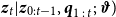 $\boldsymbol{{z}}_{t}|\boldsymbol{{z}}_{0:t-1}, \boldsymbol{{q}}_{1\,:\,t};\, \boldsymbol{\vartheta })$
. The importance weights follow
$\boldsymbol{{z}}_{t}|\boldsymbol{{z}}_{0:t-1}, \boldsymbol{{q}}_{1\,:\,t};\, \boldsymbol{\vartheta })$
. The importance weights follow
 $w_{t}\propto w_{t-1}\tilde {w}_{t}$
where the incremental importance weight
$w_{t}\propto w_{t-1}\tilde {w}_{t}$
where the incremental importance weight
 $\tilde {w}_{t}$
is given by
$\tilde {w}_{t}$
is given by
 \begin{equation} \tilde {w}_{t}=\frac {\psi ({ \boldsymbol{{q}} }_{t}|{ \boldsymbol{{z}} }_{t};{ \boldsymbol{\vartheta } })\psi ({ \boldsymbol{{z}} }_{t}|{ \boldsymbol{{z}} }_{t-1};{ \boldsymbol{\vartheta } })}{\Psi ({ \boldsymbol{{z}} }_{t}|{ \boldsymbol{{z}} }_{0:t-1},{ \boldsymbol{{q}} }_{1\,:\,t};\,{ \boldsymbol{\vartheta } })}. \end{equation}
In the numerator of (16), the first factor,
 $\psi ($
 $\boldsymbol{{q}}_{t}|\boldsymbol{{z}}_{t}; \boldsymbol{\vartheta })$
, is the probability density of observing prices and shares
$\boldsymbol{{q}}_{t}|\boldsymbol{{z}}_{t}; \boldsymbol{\vartheta })$
, is the probability density of observing prices and shares
 $\boldsymbol{{q}}_{t}$
conditional on state
$\boldsymbol{{q}}_{t}$
conditional on state
 $\boldsymbol{{z}}_{t}$
and the second factor,
$\boldsymbol{{z}}_{t}$
and the second factor,
 $\psi (\boldsymbol{{z}}_{t}|\boldsymbol{{z}}_{t-1};\boldsymbol{\vartheta })$
, is the probability density of the state transition.
$\psi (\boldsymbol{{z}}_{t}|\boldsymbol{{z}}_{t-1};\boldsymbol{\vartheta })$
, is the probability density of the state transition.
The likelihood of the state-space model can be calculated as a by-product of the filtering. An estimate of the contribution to the likelihood at time
 $t$
is
$t$
is
 \begin{equation*} \psi ({ \boldsymbol{{q}} }_{t}|{ \boldsymbol{{q}} }_{1:t-1};{ \boldsymbol{\vartheta } })=\int \psi ({ \boldsymbol{{q}} }_{t}|{ \boldsymbol{{z}} }_{t};{ \boldsymbol{\vartheta } })\psi ({ \boldsymbol{{z}} }_{t}|{ \boldsymbol{{q}} }_{1:t-1};{ \boldsymbol{\vartheta } })d{ \boldsymbol{{z}} }_{t}\approx \sum _{i=1}^{N}w_{t-1}^{(i)}\tilde {w}_{t}^{(i)} \end{equation*}
where
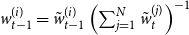 $w_{t-1}^{(i)}=\tilde {w}_{t-1}^{(i)}\left (\sum _{j=1}^{N}\tilde {w}_{t}^{(j)}\right )^{-1}$
is a normalized importance weight.
$w_{t-1}^{(i)}=\tilde {w}_{t-1}^{(i)}\left (\sum _{j=1}^{N}\tilde {w}_{t}^{(j)}\right )^{-1}$
is a normalized importance weight.
As it is well established in the literature, the sequential importance sampling suffers from the weight degeneracy, i.e. the probability masses of all but one particle converge to zero as
 $t$
increases. Therefore, the normalized importance weight of one particle converges to one while the normalized weights of the other particles converge to zero. As a result, as shown in Chopin (Reference Chopin2004), the variance of the weights grows exponentially in time and the estimator becomes a function of a single draw. Gordon et al. (Reference Gordon, Salmond and Smith1993) show that a resampling step can prevent the weight degeneracy problem. The bootstrap filter of Gordon et al. (Reference Gordon, Salmond and Smith1993) uses transition density as the proposal,
$t$
increases. Therefore, the normalized importance weight of one particle converges to one while the normalized weights of the other particles converge to zero. As a result, as shown in Chopin (Reference Chopin2004), the variance of the weights grows exponentially in time and the estimator becomes a function of a single draw. Gordon et al. (Reference Gordon, Salmond and Smith1993) show that a resampling step can prevent the weight degeneracy problem. The bootstrap filter of Gordon et al. (Reference Gordon, Salmond and Smith1993) uses transition density as the proposal,
 $\Psi ($
 $\boldsymbol{{z}}_{t}|\boldsymbol{{z}}_{t-1}, \, \boldsymbol{{q}}_{t}; \boldsymbol{\vartheta })=\psi (\boldsymbol{{z}}_{t}|\boldsymbol{{z}}_{t-1};\boldsymbol{\vartheta })$
, and does not take into account information in the current observation. Such a “blind” proposal may lead to poor performance when the observations are informative on the latent states. The class of adapted particle filters addresses this issue and incorporates
$\boldsymbol{{z}}_{t}|\boldsymbol{{z}}_{t-1}, \, \boldsymbol{{q}}_{t}; \boldsymbol{\vartheta })=\psi (\boldsymbol{{z}}_{t}|\boldsymbol{{z}}_{t-1};\boldsymbol{\vartheta })$
, and does not take into account information in the current observation. Such a “blind” proposal may lead to poor performance when the observations are informative on the latent states. The class of adapted particle filters addresses this issue and incorporates
 $\boldsymbol{{q}}_{t}$
into their proposals. The auxiliary particle filter of Pitt and Shephard (Reference Pitt and Shephard1999) is a popular algorithm that implements a fully adapted particle filter.
$\boldsymbol{{q}}_{t}$
into their proposals. The auxiliary particle filter of Pitt and Shephard (Reference Pitt and Shephard1999) is a popular algorithm that implements a fully adapted particle filter.
While resampling resolves the weight degeneracy problem, it makes the likelihood a discontinuous function of the parameters. The discontinuity problem persists even if resampling is based on common (seeded) random numbers. The discontinuity (and non-smoothness) of the log-likelihood function can cause problems for optimizers, especially for gradient-based routines – see Hurzeler and Kunsch (Reference Hurzeler, Kunsch, Hurzeler and Kunsch2001) for a discussion. Malik and Pitt (Reference Malik and Pitt2011) develop a resampling algorithm which ensures a smooth log-likelihood function in a one-dimensional case. Generalization of their method for a multivariate model is quite expensive computationally. In this paper, we take an alternative approach to preserve the smoothness of the likelihood function. At the resampling step, we draw particles from the normal distribution with moments estimated from the current particle swarm,
 $N(\mu _{z,t},\sigma _{z,t}^{2})$
where
$N(\mu _{z,t},\sigma _{z,t}^{2})$
where
 $\mu _{z,t}=N^{-1}\sum _{i=1}^{N}\tilde {w}_{t}^{(i)}z_{t}^{(i)}$
,
$\mu _{z,t}=N^{-1}\sum _{i=1}^{N}\tilde {w}_{t}^{(i)}z_{t}^{(i)}$
,
 $\sigma _{z,t}^{2}=(N-1)^{-1}\sum _{i=1}^{N}\tilde {w}_{t}^{(i)}(z_{t}^{(i)}-\mu _{z,t})^{2}$
, and
$\sigma _{z,t}^{2}=(N-1)^{-1}\sum _{i=1}^{N}\tilde {w}_{t}^{(i)}(z_{t}^{(i)}-\mu _{z,t})^{2}$
, and
 $\{\tilde {w}_{t}^{(i)}\}_{i=1}^{N}$
are normalized particle weights in period
$\{\tilde {w}_{t}^{(i)}\}_{i=1}^{N}$
are normalized particle weights in period
 $t$
. The bias that stems from this approximation is likely to be small because our model has strongly informative observations and the filtering density is localized around its mean. Similar procedures are used in Fulop and Li (Reference Fulop and Li2019) and Isakin and Ngo (Reference Isakin and Ngo2019). We present the algorithms of two versions of the particle filter: the bootstrap filter and the fully adapted auxiliary particle filter.
$t$
. The bias that stems from this approximation is likely to be small because our model has strongly informative observations and the filtering density is localized around its mean. Similar procedures are used in Fulop and Li (Reference Fulop and Li2019) and Isakin and Ngo (Reference Isakin and Ngo2019). We present the algorithms of two versions of the particle filter: the bootstrap filter and the fully adapted auxiliary particle filter.
A.1. The algorithm of the Bootstrap filter
I. In period
 $t=0$
:
$t=0$
:
-
1. Draw each set of
 $N$
particles
$\{z_{0}^{(i)}\}_{i=1}^{N}$
for the vector of unobserved prices
$p_{n0}$
from its prior distribution. Set weights of particles
$w_{0}^{(i)}=1/N$
,
$i=1,\ldots ,N$
.
$N$
particles
$\{z_{0}^{(i)}\}_{i=1}^{N}$
for the vector of unobserved prices
$p_{n0}$
from its prior distribution. Set weights of particles
$w_{0}^{(i)}=1/N$
,
$i=1,\ldots ,N$
.


II. For periods
 $t=1,\ldots ,T$
:
$t=1,\ldots ,T$
:
-
1. Update the particle weights as
where
\begin{equation*} w_{t}^{(i)}\propto \Phi \left (chol\left (\boldsymbol{\Sigma }_{\varepsilon } \right )^{-1}\left (\boldsymbol{{x}}({ \boldsymbol{{p}} }_{t}^{(i)};\boldsymbol{\vartheta })-{ \boldsymbol{{x}} }_{t}\right )\right ),\quad i=1,\ldots ,N \end{equation*}
$\Phi \left (\cdot \right )$
is the standard normal PDF,
$chol(\cdot )$
denotes the Cholesky decomposition,
$\boldsymbol{{p}}_{t}^{(i)}$
is a combined vector of observed prices in period
$t$
and
$i$
th particle for the unobserved price, and
$\boldsymbol{{x}}(\boldsymbol{{p}}_{t}^{(i)};\boldsymbol{\vartheta })$
is the vector of fitted quantities given by equation (12). At this step, the monotonicity can be imposed by setting weights to zero for the particles that violate the property.
-
2. Calculate the incremental likelihood
$\bar {w}_{t}=\frac {1}{N} \sum _{i=1}^{N}w_{t}^{(i)}$
. -
3. Calculate normalized weights
$\tilde {w}_{t}^{i}=w_{t}^{(i)}/ \sum _{i=1}^{N}w_{t}^{(i)}$
for
$i=1,\ldots ,N$
. Resample
$N$
particles
$\{z_{t}^{(i)}\}_{i=1}^{N}$
from
$N(\mu _{z,t},\sigma _{z,t}^{2})$
where
$\mu _{z,t}=N^{-1}\sum _{i=1}^{N}\tilde {w}_{t}^{(i)}z_{t}^{(i)}$
and
$\sigma _{z,t}^{2}={(N-1)^{-1}}\sum _{i=1}^{N}\tilde {w}_{t}^{(i)}(z_{t}^{(i)}-\mu _{z,t})^{2}$
. -
4. Propagate the particles using the transition equation
$\ln z_{t}^{(i)}=\ln z_{t-1}^{(i)}+v_{t}$
where
$v_{t}\sim N(0,\sigma _{v}^{2})$
.


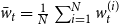


A.2. The algorithm of the fully adapted auxiliary particle filter
I. In period
 $t=0$
:
$t=0$
:
-
1. Draw each set of
$N$
particles
$\{z_{0}^{(i)}\}_{i=1}^{N}$
for the vector of unobserved prices
$p_{n0}$
from its prior distribution. Set weights of particles
$w_{0}^{(i)}=1/N$
,
$i=1,\ldots ,N$
.


II. For periods
 $t=1,\ldots ,T$
:
$t=1,\ldots ,T$
:
-
1. Reweight particles as
where
\begin{equation*} \tilde {w}_{t}^{(i)}=p\left ({ \boldsymbol{{q}} }_{t}|z_{t-1}^{(i)}\right ) \end{equation*}
$\boldsymbol{{q}}_{t}=(\boldsymbol{{p}}_{t}, \boldsymbol{{x}}_{t})$
is the pair of vectors of observed prices and quantities, and normalize weights as
$\hat {w}_{t}^{(i)}=\left (\sum _{j=1}^{N}\tilde {w} _{t}^{(j)}\right )^{-1}\tilde {w}_{t}^{(i)}$
.
-
2. Calculate normalized weights
$\tilde {w}_{t}^{i}=w_{t}^{(i)}/ \sum _{i=1}^{N}w_{t}^{(i)}$
for
$i=1,\ldots ,N$
. Resample
$N$
particles
$ \{z_{t}^{(i)}\}_{i=1}^{N}$
from
$N(\mu _{z,t},\sigma _{z,t}^{2})$
where
$ \mu _{z,t}=N^{-1}\sum _{i=1}^{N}\tilde {w}_{t}^{(i)}z_{t}^{(i)}$
and
$ \sigma _{z,t}^{2}={(N-1)^{-1}}\sum _{i=1}^{N}\tilde {w}_{t}^{(i)}(z_{t}^{(i)}- \mu _{z,t})^{2}$
. -
3. Propagate the particles using the transition equation
$\ln z_{t}^{(i)}=\ln z_{t-1}^{(i)}+v_{t}$
where
$v_{t}\sim N(0,\sigma _{v}^{2})$
.


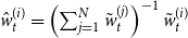


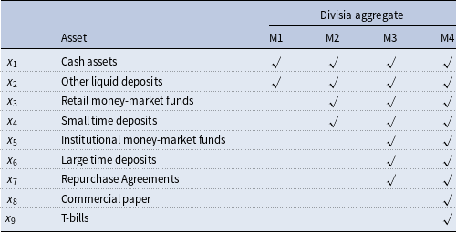
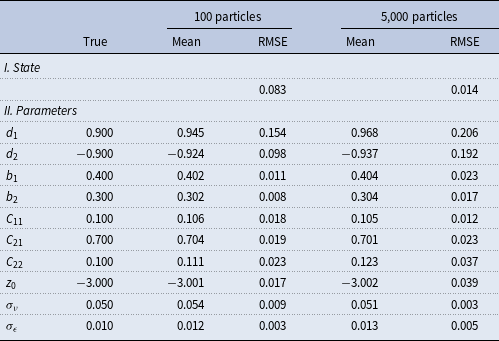
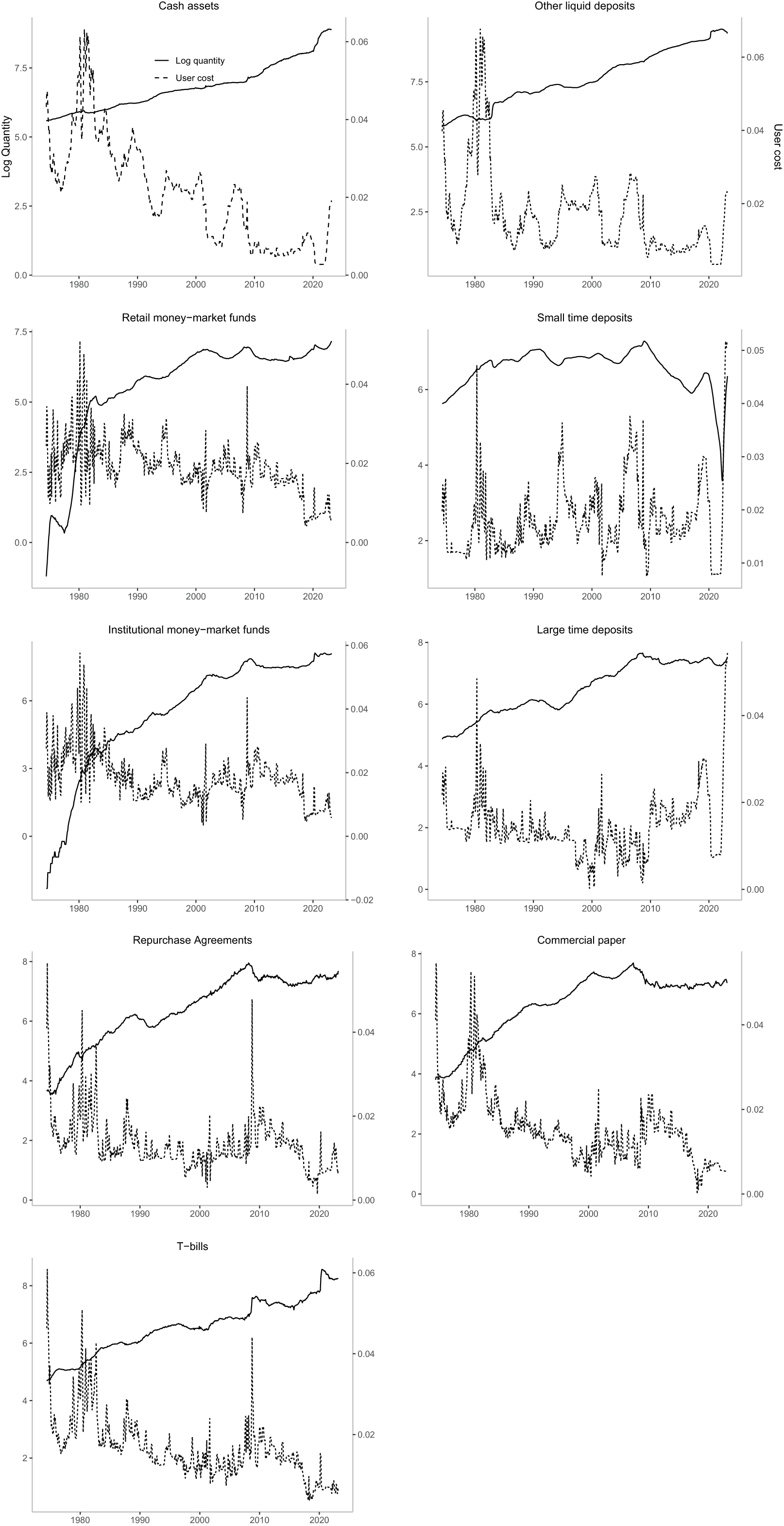
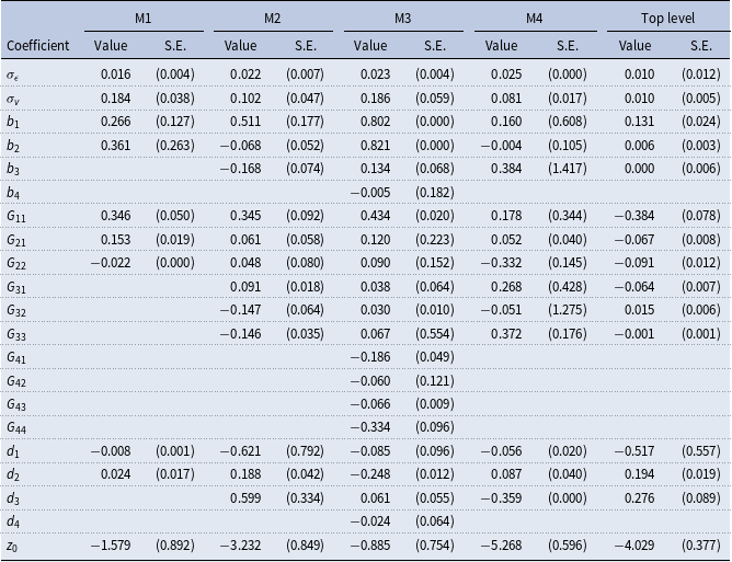


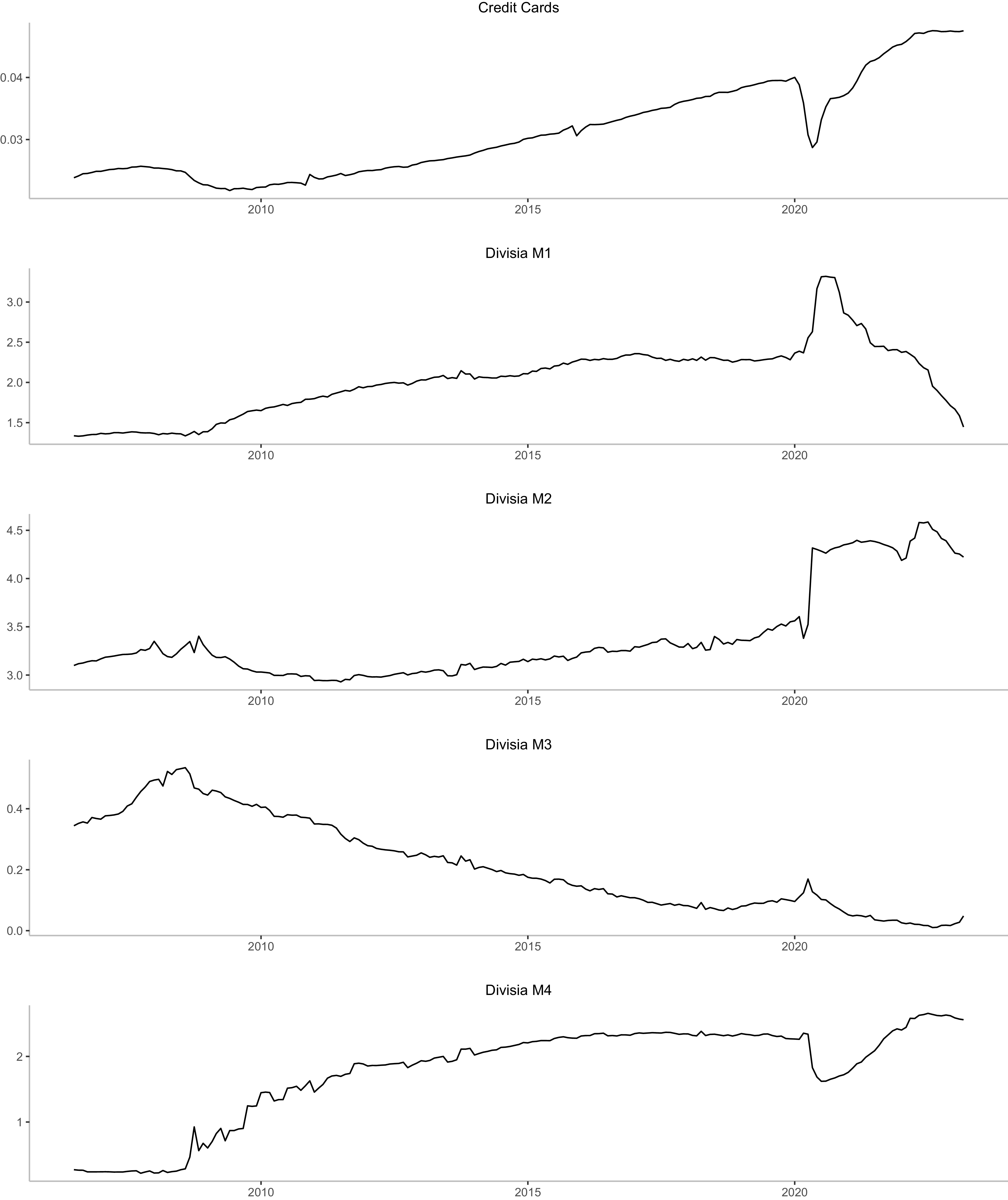
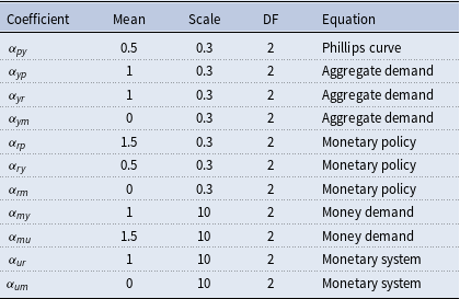
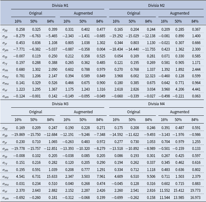


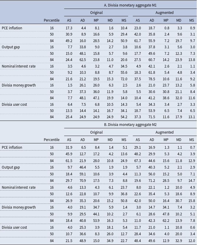

 Open access