


1. Introduction
Snow precipitated over glaciers and ice sheets transforms into ice in the uppermost layers of the ice column through firn densification. During this process, old snow is buried and compressed as a result of the overburden pressure until it reaches the density of pure ice. Understanding and modeling the details of this process is central for the interpretation of ice core records and assessing the mass balance of glaciers and ice sheets based on satellite altimetry.
In the case of ice core records, a good understanding of the air-trapping mechanism is key for interpreting gas records. The air present in firn pores becomes isolated from the atmosphere not until deep in the firn column, at the so-called bubble close-off (BCO) depth. This can create 100- to 1000-year differences in age between trapped gases and the surrounding ice (Δage), which must be considered to properly synchronize records (Schwander and others, Reference Schwander, Sowers, Barnola, Blunier, Fuchs and Malaizé1997).
In the case of mass-balance monitoring from satellite altimetry, the problem is to translate changes in altitude into changes in mass. Sea-level rise estimates can be biased if the firn density field (i.e. firn compaction) is not correctly accounted for (Sørensen and others, Reference Sorensen2011, Lipovsky, Reference Lipovsky2022), and recent efforts to include horizontal density variations over the West Antarctic ice sheet in large-scale modeling finds a correction in volume above flotation over 40 years of  $10\%$ (Schelpe and Gudmundsson, Reference Schelpe and Gudmundsson2023).
Firn densification models are an important tool that can help estimate the effect of densification on ice-core climatic records and mass-loss uncertainties. Ideally, densification models would be derived from first principles, but densification is a complex process in which crystals rearrange and change their shape and size. As a consequence, the relative importance of the different mechanisms driving densification is divided into several stages depending on local conditions (for details see Cuffey and Paterson, Reference Cuffey and Paterson2010, p. 16–22). To simplify matters, large-scale models of firn columns therefore tend to be constructed based on phenomenological arguments.
Herron and Langway (Reference Herron and Langway1980) proposed a one-dimensional empirically tuned model of the first and second stages of densification for predicting depth–density, depth–load and depth–age profiles based exclusively on local temperature and accumulation rate. Their celebrated model has since become the benchmark for comparing more sophisticated models with (e.g. Barnola and others, Reference Barnola, Pimienta, Raynaud and Korotkevich1991, Li and Zwally,Reference Li and Zwally2011). However, reproducing observed density profiles at sites with diverse climatic conditions remains challenging, and some models give inconsistent results for the same boundary conditions (Lundin and others, Reference Lundin2017), suggesting that more work is warranted.
Densification models that attempt to expand on the physical rigor of previous work have also been proposed, although improved accuracy over empirically based models does not necessarily follow (Thompson-Munson and others, Reference Thompson-Munson, Wever, Stevens, Lenaerts and Medley2023). For example, Alley (Reference Alley1987) proposed a simple model for porous firn densification by grain boundary sliding, several models make use of a one-dimensional compactive viscosity (Arnaud and others, Reference Arnaud, Barnola and Duval2000, Morris and Wingham, Reference Morris and Wingham2014, Stevens and others, Reference Stevens, Lilien, Conway, Fudge, Koutnik and Waddington2023), and three-dimensional constitutive relations exist that argue for certain viscosity functions of firn (Salamatin and others, Reference Salamatin, Lipenkov, Barnola, Hori, Duval, Hondoh and Hondoh2009, Fourteau and others, Reference Fourteau, Freitag, Malinen and Löwe2024). Finally, we note that Arthern and others (Reference Arthern, Vaughan, Rankin, Mulvaney and Thomas2010) proposed a Nabarro–Herring creep equation for porous materials that is the basis for several of the models used for altimetry corrections (Smith and others, Reference Smith2020), and SNOWPACK—a physically based land-surface snow model originally developed to support avalanche warning (Bartelt and Lehning, Reference Bartelt and Lehning2002, Lehning and others, Reference Lehning, Bartelt, Brown and Fierz2002a, Reference Lehning, Bartelt, Brown, Fierz and Satyawali2002b)—has also been successfully adapted to model near-surface firn densification (Keenan and others, Reference Keenan2021).
1.1. Beyond one-dimensional modeling
A central problem is to take into account the larger-scale ice flow, as there is evidence of accelerated firn densification when horizontal strain rates are nonzero (Kirchner and others, Reference Kirchner, Bentley and Robertson1979, Alley and Bentley, Reference Alley and Bentley1988, Riverman and others, Reference Riverman2019). This phenomenon, called strain softening, was first introduced by Alley and Bentley (Reference Alley and Bentley1988); they argued that during the second stage, densification is primarily driven by dislocation creep, which increases with the square of the effective stress. Hence, in regions where non-negligible horizontal strain rates are superimposed on the vertical firn compaction, the effective viscosity is reduced, which should, in turn, enhance densification.
Motivated by this, Oraschewski and Grinsted (Reference Oraschewski and Grinsted2022) recently extended the Herron and Langway (Reference Herron and Langway1980) model (HL) by introducing a scale factor that allows the inclusion of horizontal strain rates as a sort of forcing parameter, together with the commonly used climate variables (temperature and accumulation rate). Specifically, the densification rate derived from the classical HL model is multiplied by a scale factor that is a function of the otherwise unresolved strain rate components.
Although extensions based on Herron and Langway (Reference Herron and Langway1980) are generally computationally inexpensive, they remain one-dimensional. Multidimensional approximations can be constructed by horizontally joining firn-column models (e.g. Oraschewski and Grinsted, Reference Oraschewski and Grinsted2022), but formulating firn densification in terms of a three-dimensional constitutive stress–strain rate relationship is desirable for several reasons: (i) the effect of nonzero horizontal strain rates can be represented naturally (without the need for any ad hoc inclusion), (ii) two- or three-dimensional firn compaction problems can be more easily solved for complicated boundary conditions and geometries using, e.g. the finite element method and (iii) Glen’s flow law for solid ice may be extended to also characterize porous firn, thereby allowing for a seamless numerical treatment of the entire firn–ice column.
The semi-empirical rheology proposed by Gagliardini and Meyssonnier (Reference Gagliardini and Meyssonnier1997)—henceforth GM97—is exactly such a field formulation. It is based on a general compressible power-law rheology for porous materials, adapted to fit in situ measured density profiles from Site-2, Greenland (see Fig. 2), and cold room deformation tests. The GM97 rheology has previously been shown capable of reproducing age–depth profiles of mountain glaciers (Lüthi and Funk, Reference Lüthi and Funk2000, Zwinger and others, Reference Zwinger, Greve, Gagliardini, Shiraiwa and Lyly2007, Gilbert and others, Reference Gilbert, Gagliardini, Vincent and Wagnon2014, Licciulli and others, Reference Licciulli, Bohleber, Lier, Gagliardini, Hoelzle and Eisen2020) and predicting the evolution of snow caves buried over time in Antarctica (Brondex and others, Reference Brondex, Gagliardini, Gillet-Chaulet and Chekki2020).
The GM97 rheology depends on two coefficient functions of density that determine the local compressibility and viscosity. The functional form of these, and associated calibration constants, have received little attention in the literature apart from the initial treatment by Gagliardini and Meyssonnier (Reference Gagliardini and Meyssonnier1997) and subsequently by Zwinger and others (Reference Zwinger, Greve, Gagliardini, Shiraiwa and Lyly2007). The proposed coefficient functions mainly disagree for near-surface firn densities, which can have a large impact on modeled surface velocities and densification rates (Gilbert and others, Reference Gilbert, Gagliardini, Vincent and Wagnon2014). This has led to some disagreement in the literature about which coefficient functions to use. More work is therefore warranted to make clear whether the calibrations proposed by Gagliardini and Meyssonnier (Reference Gagliardini and Meyssonnier1997) and Zwinger and others (Reference Zwinger, Greve, Gagliardini, Shiraiwa and Lyly2007) (i) hold for a wider range of sites, where firn cores have since been drilled and (ii) hold in two-dimensional settings, where nontrivial densification fields have been observed. If so, this would put the GM97 rheology on stronger empirical grounds and increase confidence in its future use, which is the primary aim of our work.
In this paper, we test the flexibility and usefulness of the GM97 rheology for modeling firn compaction beyond one-dimensional problems. First, we revisit the original calibration of the rheology and assess the universality of it by trying to reproduce five additional Greenlandic ice core sites, where one-dimensional modeling is appropriate. Then, we test the model’s accuracy and dependency on temperature by attempting to reproduce the collapse of a near-surface snow cave, constructed at the NEEM ice core site in Greenland. Finally, we test whether the rheology can reproduce the enhanced densification observed at the shear margins of the Northeast Greenland Ice Stream (NEGIS), believed to be caused by strain-softening effects. In the following, we begin by introducing the GM97 rheology before considering the special one- and two-dimensional cases thereof, needed for our experiments.
2. Method
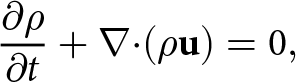
For a compressible material, mass conservation implies that
 \begin{equation}
\frac{\partial\rho}{\partial t} + {\boldsymbol\nabla}{\boldsymbol\cdot}(\rho{\mathbf{u}}) = 0
,
\end{equation}
\begin{equation}
\frac{\partial\rho}{\partial t} + {\boldsymbol\nabla}{\boldsymbol\cdot}(\rho{\mathbf{u}}) = 0
,
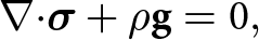
\end{equation}where u and ρ are the velocity and density fields, respectively. The velocity field of a Stokes fluid is governed by the momentum balance
 \begin{equation}
{\boldsymbol\nabla}{\boldsymbol\cdot}{\boldsymbol{\sigma}} + \rho {\mathbf{g}} = {{0}},
\end{equation}
\begin{equation}
{\boldsymbol\nabla}{\boldsymbol\cdot}{\boldsymbol{\sigma}} + \rho {\mathbf{g}} = {{0}},
\end{equation} where  $\boldsymbol{\sigma}(\dot{\boldsymbol{\epsilon}})$ is the stress tensor, $\dot{\boldsymbol{\epsilon}}=({\boldsymbol\nabla}{\mathbf{u}} + ({\boldsymbol\nabla}{\mathbf{u}})^{\mathsf{T}})/2$ is the strain rate tensor and g is the gravitational acceleration vector.
The GM97 rheology treats firn densification as a secondary creep problem involving u, ρ and the temperature (or enthalpy) T, assuming negligible effects from primary creep, snow metamorphism and the brittle fracturing of snow. The rheology represents both firn and ice using a single, compressible Norton–Bailey power-law fluid that conforms to Glen’s incompressible flow law in the limit  $\rho \rightarrow \rho_{\mathrm{ice}}$, where $\rho_{\mathrm{ice}}=917\,\text{kg}\,\text{m}^{-3}$ is the density of glacier ice. The rheology is to be understood as an extension of Glen’s flow law that depends on the first invariant of the strain rate tensor, $\mathrm{tr}(\dot{\boldsymbol{\epsilon}})$, in addition to the usual second invariant,
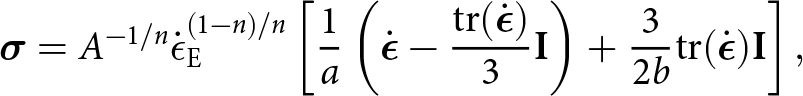
  $\dot{\boldsymbol{\epsilon}}:\dot{\boldsymbol{\epsilon}}$. The rheology was first proposed by Duva and Crow (Reference Duva and Crow1994) for general porous materials but has since been adopted in glaciology, and recently with renewed interest (Brondex and others, Reference Brondex, Gagliardini, Gillet-Chaulet and Chekki2020, Licciulli and others, Reference Licciulli, Bohleber, Lier, Gagliardini, Hoelzle and Eisen2020). Written in its inverse form (see Appendix B) required by the momentum balance (2), the rheology is
 \begin{equation}
\boldsymbol{\sigma} = A^{-1/n} \dot{\epsilon}_{\mathrm{E}}^{(1-n)/n}\left[\frac{1}{a}\left(\dot{\boldsymbol{\epsilon}} - \frac{\mathrm{tr}(\dot{\boldsymbol{\epsilon}})}{3}{\mathbf{I}}\right) + \frac{3}{2b}\mathrm{tr}(\dot{\boldsymbol{\epsilon}}){\mathbf{I}}\right],
\end{equation}
\begin{equation}
\boldsymbol{\sigma} = A^{-1/n} \dot{\epsilon}_{\mathrm{E}}^{(1-n)/n}\left[\frac{1}{a}\left(\dot{\boldsymbol{\epsilon}} - \frac{\mathrm{tr}(\dot{\boldsymbol{\epsilon}})}{3}{\mathbf{I}}\right) + \frac{3}{2b}\mathrm{tr}(\dot{\boldsymbol{\epsilon}}){\mathbf{I}}\right],
\end{equation}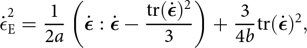 \begin{equation}
\dot{\epsilon}_{\mathrm{E}}^2 = \frac{1}{2a}\left(\dot{\boldsymbol{\epsilon}}:\dot{\boldsymbol{\epsilon}} - \frac{\mathrm{tr}(\dot{\boldsymbol{\epsilon}})^2}{3}\right) + \frac{3}{4b}\mathrm{tr}(\dot{\boldsymbol{\epsilon}})^2,
\end{equation}
\begin{equation}
\dot{\epsilon}_{\mathrm{E}}^2 = \frac{1}{2a}\left(\dot{\boldsymbol{\epsilon}}:\dot{\boldsymbol{\epsilon}} - \frac{\mathrm{tr}(\dot{\boldsymbol{\epsilon}})^2}{3}\right) + \frac{3}{4b}\mathrm{tr}(\dot{\boldsymbol{\epsilon}})^2,
\end{equation} where n = 3 following the above-mentioned adoptions of the rheology,  $\dot{\epsilon}_{\mathrm{E}}$ is the effective strain rate and a and b are the coefficient functions controlling firn viscosity and compressibility (elaborated on below). Note here that Glen’s law is recovered when a = 1, b = 0 and $\mathrm{tr}(\dot{\boldsymbol{\epsilon}}) = 0$, which must be fulfilled in the limit $\rho\rightarrow \rho_{\mathrm{ice}}$.
Since the flow-rate factor, A, depends on temperature, the evolution of the temperature field (T) needs to be considered, too:
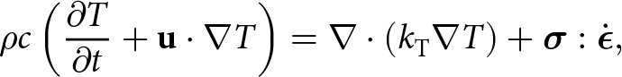 \begin{equation}\rho c\left(\frac{\partial T}{\partial t}+\mathbf u\boldsymbol\cdot\boldsymbol\nabla T\right)=\boldsymbol\nabla\boldsymbol\cdot(k_{\mathrm T}\boldsymbol\nabla T)+\boldsymbol\sigma:\dot{\boldsymbol\epsilon},\end{equation}
 where  $c=c(T)$ and ${k_{\mathrm{T}}}={k_{\mathrm{T}}}(T,\rho)$ are the specific heat capacity and thermal conductivity of ice (see Appendix A for empirical functional forms used). In GM97, the flow-rate factor is modeled the usual way as an Arrhenius activation function of temperature (Greve and Blatter, Reference Greve and Blatter2009, Greve and others, Reference Greve, Zwinger and Gong2014):
 \begin{equation}
A(T) = A_0 \exp[-Q/(RT)],
\end{equation}
\begin{equation}
A(T) = A_0 \exp[-Q/(RT)],
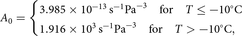
\end{equation}where, following Zwinger and others (Reference Zwinger, Greve, Gagliardini, Shiraiwa and Lyly2007), the canonical dependence on the temperature of the prefactor A 0 and the activation energy for creep, Q, are presumed:
 \begin{equation}
A_0 =
\begin{cases}
3.985 \times 10^{-13}\,\text{s}^{-1} \text{Pa}^{-3} {\quad\text{for}\quad} T \leq -10{^\circ}\text{C} \\
1.916 \times 10^{3}\,\text{s}^{-1} \text{Pa}^{-3} {\quad\text{for}\quad} T \gt -10{^\circ}\text{C}
,
\end{cases}
\end{equation}
\begin{equation}
A_0 =
\begin{cases}
3.985 \times 10^{-13}\,\text{s}^{-1} \text{Pa}^{-3} {\quad\text{for}\quad} T \leq -10{^\circ}\text{C} \\
1.916 \times 10^{3}\,\text{s}^{-1} \text{Pa}^{-3} {\quad\text{for}\quad} T \gt -10{^\circ}\text{C}
,
\end{cases}
\end{equation}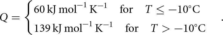 \begin{equation}
Q = \begin{cases}
60\,\text{kJ}\,\text{mol}^{-1}\,\text{K}^{-1} {\quad\text{for}\quad} T \leq -10{^\circ}\text{C} \\
139\,\text{kJ}\,\text{mol}^{-1}\,\text{K}^{-1} {\quad\text{for}\quad} T \gt -10{^\circ}\text{C}
\end{cases}.
\end{equation}
\begin{equation}
Q = \begin{cases}
60\,\text{kJ}\,\text{mol}^{-1}\,\text{K}^{-1} {\quad\text{for}\quad} T \leq -10{^\circ}\text{C} \\
139\,\text{kJ}\,\text{mol}^{-1}\,\text{K}^{-1} {\quad\text{for}\quad} T \gt -10{^\circ}\text{C}
\end{cases}.
\end{equation}The fluidity also depends on other factors such as pressure (Weertman, Reference Weertman1983), water content (Barnes and others, Reference Barnes, Tabor and Walker1971, Duval, Reference Duval1977), impurities (Hörhold and others, Reference Hörhold, Laepple, Freitag, Bigler, Fischer and Kipfstuhl2012) and grain sizes and orientations (Duval, Reference Duval1973, Shoji and Langway, Reference Shoji and Langway1988). The pressure dependence is estimated to be relatively small, even at hydrostatic pressures near ice sheet beds, and therefore neglected (Rigsby, Reference Rigsby1958). Regarding water content, temperatures are generally considered to be low enough to neglect the presence of liquid water. Impurities, such as dust, are known to increase ice softness by up to a factor of two, but in the Greenland firn column considered here—which consists only of Holocene deposition—the dust loading is minimal or can at least be assumed to be uniform to first order. Finally, changes in the size and orientation of grains are thought to be important in dynamic regions such as ice streams and their shear margins (e.g. Gerber and others, Reference Gerber2021), but expanding (3)–(4) to also allow for viscous anisotropy is a daunting task and out of scope of this work, so the effect of developed crystal fabrics in the firn constitute a rheological uncertainty throughout this work.
2.1. Coefficient functions
Following Duva and Crow (Reference Duva and Crow1994), the coefficient functions a and b are taken to depend exclusively on the relative density
 \begin{equation}
{\hat{\rho}} = \frac{\rho}{\rho_{\mathrm{ice}}}.
\end{equation}
\begin{equation}
{\hat{\rho}} = \frac{\rho}{\rho_{\mathrm{ice}}}.
\end{equation} In this way, if a and b are affected by temperature, grain sizes, etc., it is implicitly assumed that such dependencies can be factored out and absorbed into A. Indeed, this separation of dependencies is desirable since (3)–(4) can then be easily made to reduce to Glen’s law in the limit  ${\hat{\rho}}\rightarrow 1$, as noted above.
The coefficient functions a and b depend in part on a model for how stresses concentrate in the presence of enclosed voids (air) (Duva and Crow, Reference Duva and Crow1994) for densities above the critical value  ${\hat{\rho}}\geq {\hat{\rho}}_{\mathrm{crit}} = 0.81$:
 \begin{equation}
a_0 = \frac{1+\frac{2}{3}(1-{\hat{\rho}})}{{\hat{\rho}}^{2n/(n+1)}} ,
\end{equation}
\begin{equation}
a_0 = \frac{1+\frac{2}{3}(1-{\hat{\rho}})}{{\hat{\rho}}^{2n/(n+1)}} ,
\end{equation} \begin{equation}
b_0 = \frac{3}{4}\left( \frac{n^{-1} (1-{\hat{\rho}})^{1/n}}{1-(1-{\hat{\rho}})^{1/n}} \right)^{2n/(n+1)}
,
\end{equation}
\begin{equation}
b_0 = \frac{3}{4}\left( \frac{n^{-1} (1-{\hat{\rho}})^{1/n}}{1-(1-{\hat{\rho}})^{1/n}} \right)^{2n/(n+1)}
,
\end{equation} and in part on an empirical scaling relation for densities  ${\hat{\rho}} \lt {\hat{\rho}}_{\mathrm{crit}}$ that has been found to fit cold room experiments and densification measured at Site 2, Greenland. Specifically, two such sets of a and b scalings have been proposed: Gagliardini and Meyssonnier (Reference Gagliardini and Meyssonnier1997) suggested (Fig. 1, dashed lines)
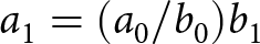 \begin{equation}
a_1 = (a_0/b_0) b_1
\end{equation}
\begin{equation}
a_1 = (a_0/b_0) b_1
\end{equation}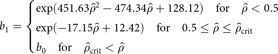 \begin{equation}
b_1 = \begin{cases}
\exp(451.63{\hat{\rho}}^2-474.34{\hat{\rho}} + 128.12) {\quad\text{for}\quad} {\hat{\rho}} \lt 0.5 \\
\exp(-17.15{\hat{\rho}} + 12.42) {\quad\text{for}\quad} 0.5 \leq {\hat{\rho}} \leq {\hat{\rho}}_{\mathrm{crit}} \\
b_0 {\quad\text{for}\quad} {\hat{\rho}}_{\mathrm{crit}} \lt {\hat{\rho}}
\end{cases}
\end{equation}
\begin{equation}
b_1 = \begin{cases}
\exp(451.63{\hat{\rho}}^2-474.34{\hat{\rho}} + 128.12) {\quad\text{for}\quad} {\hat{\rho}} \lt 0.5 \\
\exp(-17.15{\hat{\rho}} + 12.42) {\quad\text{for}\quad} 0.5 \leq {\hat{\rho}} \leq {\hat{\rho}}_{\mathrm{crit}} \\
b_0 {\quad\text{for}\quad} {\hat{\rho}}_{\mathrm{crit}} \lt {\hat{\rho}}
\end{cases}
\end{equation}Coefficient functions a (red) and b (blue) proposed by Gagliardini and Meyssonnier (Reference Gagliardini and Meyssonnier1997) and Zwinger and others (Reference Zwinger, Greve, Gagliardini, Shiraiwa and Lyly2007) for n = 3.
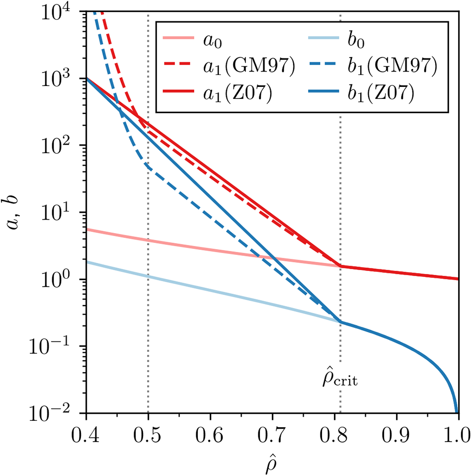
whereas Zwinger and others (Reference Zwinger, Greve, Gagliardini, Shiraiwa and Lyly2007) suggested (Fig. 1, dark solid lines)
 \begin{equation}
a_1 =
\begin{cases}
k_a \exp\normalsize(-\gamma_{a}({\hat{\rho}}-{\hat{\rho}}_{\mathrm{sfc}})\normalsize) {\quad\text{for}\quad} {\hat{\rho}} \leq {\hat{\rho}}_{\mathrm{crit}} \\
a_0 {\quad\text{for}\quad} {\hat{\rho}}_{\mathrm{crit}} \lt {\hat{\rho}}
\end{cases}
\end{equation}
\begin{equation}
a_1 =
\begin{cases}
k_a \exp\normalsize(-\gamma_{a}({\hat{\rho}}-{\hat{\rho}}_{\mathrm{sfc}})\normalsize) {\quad\text{for}\quad} {\hat{\rho}} \leq {\hat{\rho}}_{\mathrm{crit}} \\
a_0 {\quad\text{for}\quad} {\hat{\rho}}_{\mathrm{crit}} \lt {\hat{\rho}}
\end{cases}
\end{equation}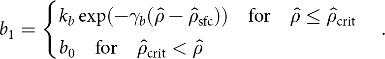 \begin{equation}
b_1 =
\begin{cases}
k_b \exp\normalsize(-\gamma_{b}({\hat{\rho}}-{\hat{\rho}}_{\mathrm{sfc}})\normalsize) {\quad\text{for}\quad} {\hat{\rho}} \leq {\hat{\rho}}_{\mathrm{crit}} \\
b_0 {\quad\text{for}\quad} {\hat{\rho}}_{\mathrm{crit}} \lt {\hat{\rho}}
\end{cases}.
\end{equation}
\begin{equation}
b_1 =
\begin{cases}
k_b \exp\normalsize(-\gamma_{b}({\hat{\rho}}-{\hat{\rho}}_{\mathrm{sfc}})\normalsize) {\quad\text{for}\quad} {\hat{\rho}} \leq {\hat{\rho}}_{\mathrm{crit}} \\
b_0 {\quad\text{for}\quad} {\hat{\rho}}_{\mathrm{crit}} \lt {\hat{\rho}}
\end{cases}.
\end{equation} Here  ${\hat{\rho}}_{\mathrm{sfc}}=0.4$ is the assumed relative density of surface snow, continuity at ${\hat{\rho}}={\hat{\rho}}_{\mathrm{crit}}$ implies the scaling exponents are
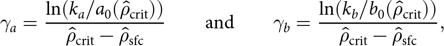 \begin{equation}
\gamma_a = \frac{\ln(k_a/a_0({\hat{\rho}}_{\mathrm{crit}})) }{{\hat{\rho}}_{\mathrm{crit}}-{\hat{\rho}}_{\mathrm{sfc}}}
\qquad \text{and} \qquad
\gamma_b = \frac{\ln(k_b/b_0({\hat{\rho}}_{\mathrm{crit}})) }{{\hat{\rho}}_{\mathrm{crit}}-{\hat{\rho}}_{\mathrm{sfc}}} ,
\end{equation}
\begin{equation}
\gamma_a = \frac{\ln(k_a/a_0({\hat{\rho}}_{\mathrm{crit}})) }{{\hat{\rho}}_{\mathrm{crit}}-{\hat{\rho}}_{\mathrm{sfc}}}
\qquad \text{and} \qquad
\gamma_b = \frac{\ln(k_b/b_0({\hat{\rho}}_{\mathrm{crit}})) }{{\hat{\rho}}_{\mathrm{crit}}-{\hat{\rho}}_{\mathrm{sfc}}} ,
\end{equation}and ka and kb are parameters to be calibrated against observations or experiments, suggested by Zwinger and others (Reference Zwinger, Greve, Gagliardini, Shiraiwa and Lyly2007) to be
 \begin{equation}
k \equiv k_a=k_b \simeq 1000.
\end{equation}
\begin{equation}
k \equiv k_a=k_b \simeq 1000.
\end{equation} Note that ka and kb are the values of a and b at the surface,  ${\hat{\rho}}={\hat{\rho}}_{\mathrm{sfc}}$.
As pointed out by Brondex and others (Reference Brondex, Gagliardini, Gillet-Chaulet and Chekki2020), ka and kb should ideally be re-calibrated on a case-by-case basis, although adopting the cold room and Site 2 calibration proposed by Zwinger and others (Reference Zwinger, Greve, Gagliardini, Shiraiwa and Lyly2007) ( $k \simeq 1000$) has been found sufficient in several cases (Gilbert and others, Reference Gilbert, Gagliardini, Vincent and Wagnon2014, Brondex and others, Reference Brondex, Gagliardini, Gillet-Chaulet and Chekki2020, Licciulli and others, Reference Licciulli, Bohleber, Lier, Gagliardini, Hoelzle and Eisen2020) and is regarded as the canonical value. In this work, we revisit the best-fit value of k by considering additional one- and two-dimensional model experiments that are evaluated against observations.
2.2. Numerics
In the numerical experiments that follow, we solved the coupled density, momentum and thermal problem using FEniCS (Logg and others, Reference Logg, Mardal and Wells2012), relying on Newton’s method to solve nonlinearities. For reasons explained below, the ice stream scenario is not thermally coupled, but the mechanical problem is solved using the same method. The Jacobian of the residual forms (required for Newton iterations) were calculated using the unified form language (Alnæs and others, Reference Alnæs2015), used by FEniCS to specify weak forms of partial differential equations (PDEs), which supports automatic symbolic differentiation. All weak forms are presented in Appendix A.
For our two-dimensional experiments, meshes were constructed using gmsh (Geuzaine and Remacle, Reference Geuzaine and Remacle2009) and updated between time steps to evolve the interior and exterior free-surface boundary.
3. Validation of rheology
We considered three independent numerical experiments to test the proposed best-fit value of the calibration constant,  $k \simeq 1000$ (Zwinger and others, Reference Zwinger, Greve, Gagliardini, Shiraiwa and Lyly2007). First, we swept over k to determine which value can best reproduce observed firn density profiles from a wider range of Greenlandic ice core drill sites (case 1). Second, we sought a value of k that could best reproduce the measured collapse of a trench constructed at NEEM (Steffensen, Reference Steffensen2014) (case 2). Third, we attempted to reproduce the observed enhanced densification over the shear margins of NEGIS by varying k (case 3).
3.1. Case 1: Reproducing Greenlandic ice cores
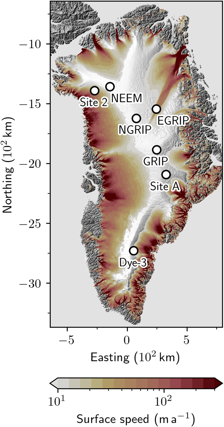
We considered a total of six Greenlandic firn cores from the deep drilling sites at DYE-3, GRIP, NGRIP, NEEM, Site 2 and Site A (Fig. 2). Since firn temperatures are approximately depth-constant at each site (Bréant and others (Reference Bréant, Martinerie, Orsi, Arnaud and Landais2017); Table 1), the problem reduces to that of solving for ρ and the vertical velocity uz if the density and velocity fields are approximated as horizontally homogeneous (similar to traditional one-dimensional modeling, although this assumption might be less well justified at dynamic sites). Unlike the transient two-dimensional problems considered in the following, we solved directly for the steady states of (1)–(2) subject to the boundary conditions
 \begin{equation}
\rho(z=0) = \rho_{\mathrm{sfc}},
\end{equation}
\begin{equation}
\rho(z=0) = \rho_{\mathrm{sfc}},
\end{equation} \begin{equation}
u_z(z=0) = -\dot{a},
\end{equation}
\begin{equation}
u_z(z=0) = -\dot{a},
\end{equation} \begin{equation}
u_z(z=-H) = -\dot{a} \frac{\rho_{\mathrm{sfc}}}{\rho_{\mathrm{ice}}},
\end{equation}
\begin{equation}
u_z(z=-H) = -\dot{a} \frac{\rho_{\mathrm{sfc}}}{\rho_{\mathrm{ice}}},
\end{equation}Sites of Greenlandic ice cores used to validate the GM97 rheology and determine k. Satellite-derived velocities from the MEaSUREs program are shown in colored contours (Howat, Reference Howat2020).
Depth-averaged temperature, accumulation rate, and surface density of each site considered. Accumulation rates and surface densities follow from Bréant and others (Reference Bréant, Martinerie, Orsi, Arnaud and Landais2017). For EGRIP, the accumulation rate and surface density data are retrieved from Karlsson and others (Reference Karlsson2020) and Schaller and others (Reference Schaller, Freitag, Kipfstuhl, Laepple, Steen-Larsen and Eisen2016), respectively.

* Average surface temperature was used due to the lack of a temperature profile.
where H is the height of the modeled firn column,  $\rho_{\mathrm{sfc}}$ is the surface snow density and $\dot{a}$ is the snow accumulation rate at the site (Table 1). The boundary condition (20) assumes that, in steady state, the mass flux into the firn column equals that exiting the column, where H must be taken sufficiently large to guarantee that the bottom of the model domain is pure ice, $\rho(z=-H) = \rho_{\mathrm{ice}}$.
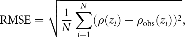
We determined the best-fit value of k by sweeping a wide range of values and calculating the resulting model–observation misfit. Specifically, we considered  $k\in [1;1000]$ and calculated the root-mean-square-error (RMSE) between the modeled and observed density profiles:
 \begin{equation}
\text{RMSE} = \sqrt{\frac{1}{N} \sum_{i=1}^{N} (\rho(z_i) - \rho_{\mathrm{obs}}(z_i))^2},
\end{equation}
\begin{equation}
\text{RMSE} = \sqrt{\frac{1}{N} \sum_{i=1}^{N} (\rho(z_i) - \rho_{\mathrm{obs}}(z_i))^2},
\end{equation}where N is the total number of discrete depth levels at which the misfit is evaluated. Computing the percentage error of each level is also an option (weighing the mismatch with respect to the reference value it is deviating from), but the results obtained in this way are virtually identical (data not shown).
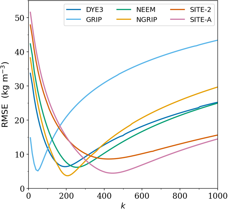
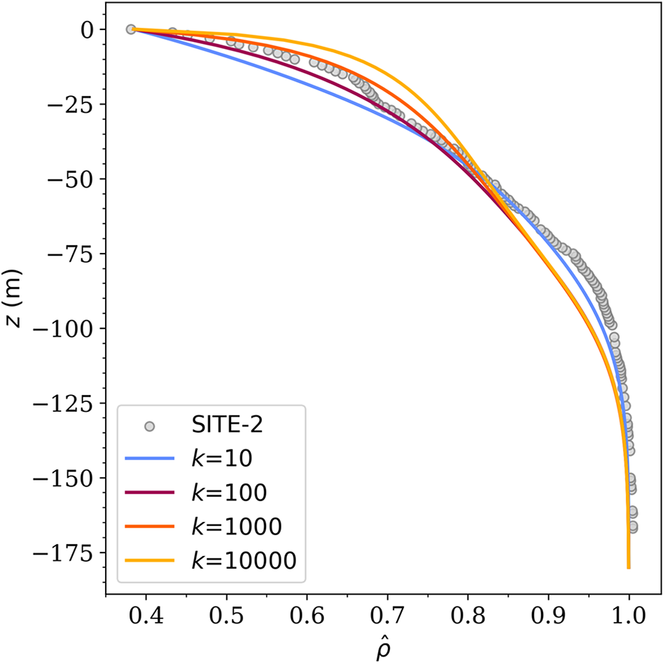
Fig. 3 shows the RMSE misfits calculated for the lower-density section of the firn column ( $\hat{\rho} \lt 0.8$), where k is expected to have the largest influence (see the above section on the coefficient functions). The results suggest a misfit minimum exists somewhere between k = 100 and k = 500 but with disagreements between the sites; that is, a global best-fit k might not be strictly applicable across all sites (disregarding effects from seasonal temperature variations not treated here for simplicity). For reference, Fig. 4 shows the model performance in the case of Site 2 for different values of k. Note that the sensitivity to the magnitude of k decreases for relative densities above 0.8. The underestimation of density at depth is present in all the sites modeled.
Model–observation RMSE of Greenlandic density profiles for  $k\in [1,1000]$. All the curves keep increasing monotonically from k = 1000 and onwards (not shown).
Modeled Site 2 density profiles for various k (colored lines) compared to observations (Bréant and others (Reference Bréant, Martinerie, Orsi, Arnaud and Landais2017); gray dots). The effect of a given k is most evident near the surface: the higher the value of k, the faster the near-surface densification. For  $\hat{\rho} \gt 0.8$, the model generally underestimates densities at a given depth for all k.
3.2. Case 2: Trench collapse at NEEM
In an attempt to further characterize the model dependence on k, we searched for alternative validation experiments that involve near-surface (low-density) firn, since the choice of k affects compressibility the most there. We found that the observed collapse of a cylindrical subsurface tunnel, constructed at the NEEM ice core site, is well-suited for this purpose.
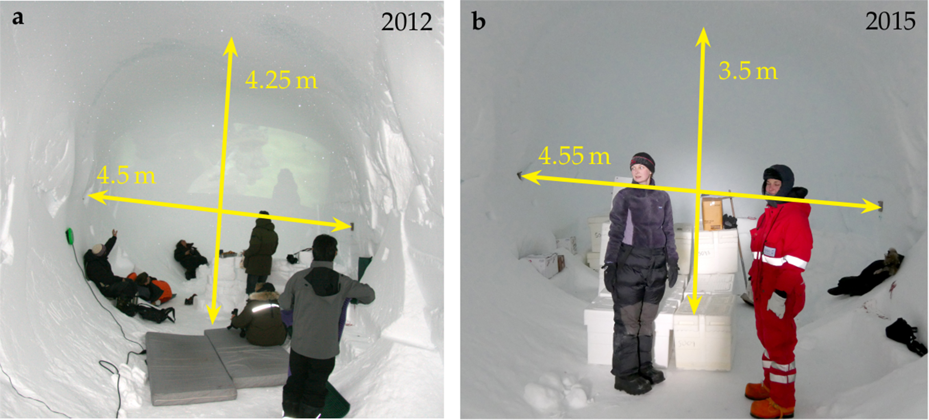
The tunnel was constructed to determine whether subsurface trenches, built following the Camp Century snow-blowing casting technique (Clark, Reference Clark1965), but using large inflatable balloons instead, could serve as drilling and science trenches for deep ice core projects. To judge its feasibility, the tunnel collapse rate was tracked for 3 years after its construction. The initial and final geometries are shown in Fig. 5 for reference, although the pictures are from the northern end of the trench, while we modeled the southern end where measurements were made most consistently.
NEEM balloon trench geometry 2 months after construction on 7 August 2012 (a) and 3 years later on 27 May 2015 (b). No picture of the trench was available for the model target year, 2014, so 2015 is shown instead. Moreover, pictures show the northern end, whereas we used the trench geometry of the southern end that was most consistently measured during the experiment (no pictures available). Pictures were kindly provided by J. P. Steffensen and reprinted with permission according to the NEEM ice-core project media waiver.
The tunnel was constructed by blowing snow out of a large trench and installing an inflatable balloon in the open cavity. After inflating it, snow was blown back into the trench again, burying the balloon in a more closely packed (denser) firn with a typical density of  $\rho_{\mathrm{trench}} = 550\,\text{kg}\,\text{m}^{-3}$ (Brondex and others, Reference Brondex, Gagliardini, Gillet-Chaulet and Chekki2020, Steffensen, Reference Steffensen2022). Finally, after a couple of days, the balloon was deflated and removed, preserving the casted, circular structure of the tunnel.
We simplify the trench collapse problem by considering a vertical cross-section model, thus implicitly assuming translational invariance along the tunnel (strictly speaking, only relevant for very long tunnels). The initial geometry and density field (Fig. 6) was constructed following the technical report by Steffensen (Reference Steffensen2014) and subsequently allowed to evolve thermomechanically throughout the duration of the test, approximately 2 years long. Note that the roof includes the reported extra 1 m of backfilled snow, but that the presence of other structures in the trench (connecting tunnels, cabins, etc.) is not considered here, which might change results slightly and are a source of uncertainty.
Zoom-in of the initial geometry and density field of the NEEM trench model. High-density snow was backfilled into the balloon trench, creating a hardened shell surrounding the tunnel compared to the background density field.
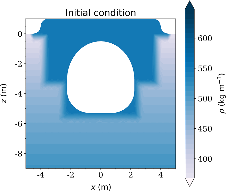
The initial background density field is taken to be equal to the smoothed density profile of the NEEM core (Bréant and others, Reference Bréant, Martinerie, Orsi, Arnaud and Landais2017). The snow accumulation rate is set to the annual average over the trench, which is double the reference measurement at NEEM due to wind-driven excess accumulation (Steffensen, Reference Steffensen2014). The initial temperature field is taken to be uniform and equal to the firn column average measured at NEEM,  $\langle T_{\mathrm{NEEM}}\rangle$ (Table 1). However, during the 5 days that it took to construct the tunnel, both the trench and the snow to be backfilled were exposed to higher-than-usual temperatures (between −3 and $-6{^\circ}\text{C}$; Steffensen (Reference Steffensen2014)). Thus, the initial temperature of the firn that surrounded the tunnel was possibly up to $25{^\circ}\text{C}$ warmer than the firn-average-background temperature (most likely less, though). In order to assess the potential underestimation of the initial collapse rate, caused by prescribing too cold firn, we therefore also consider a second scenario in which all the backfilled snow starts out with a temperature of $-5{^\circ}\text{C}$. This is just an approximation and does not intend to accurately represent the initial temperature field but rather allows us to gauge the impact that a much hotter trench might have on our results.
The model domain has a width of  $L=20\,\text{m}$ and a time-evolving height profile $h(x,t)$ relative to a fixed bottom boundary located at a depth of $H=30\,\text{m}$ below the initial surface. Both L and H are large enough to avoid boundary conditions affecting the solution (judged by trial and error). The bottom boundary is fixed by a free slip condition and kept at the site’s depth-averaged firn temperature. At the surface, we thermally force the model by setting the firn surface temperature equal to measurements from the local Greenland Climatic Network weather station, $T_{\mathrm{GCnet}}(t)$ (Vandecrux and others, Reference Vandecrux2023). To estimate the impact of not taking the surface temperature evolution into account, we also ran the model by forcing it with a constant firn surface temperature, set equal to the average measured surface temperature over the modeled period, $\langle{T_{\mathrm{GCnet}}(t)}\rangle$. A periodic boundary condition is imposed on the left and right sides to close the thermal problem.
In summary, the boundary conditions are
 \begin{equation}
u_z(x,z=-H)= 0,
\end{equation}
\begin{equation}
u_z(x,z=-H)= 0,
\end{equation} \begin{equation}
T(x,z=-H)= T_{\mathrm{icecore}}(z=-H),
\end{equation}
\begin{equation}
T(x,z=-H)= T_{\mathrm{icecore}}(z=-H),
\end{equation}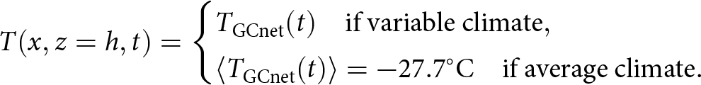 \begin{equation}
T(x,z=h,t)=
\begin{cases}
T_{\mathrm{GCnet}}(t) \quad \mathrm{if\ variable\ climate} , \\
\langle{T_{\mathrm{GCnet}}(t)}\rangle=-27.7{^\circ}\text{C} \quad \mathrm{if\ average\ climate}.
\end{cases}
\end{equation}
\begin{equation}
T(x,z=h,t)=
\begin{cases}
T_{\mathrm{GCnet}}(t) \quad \mathrm{if\ variable\ climate} , \\
\langle{T_{\mathrm{GCnet}}(t)}\rangle=-27.7{^\circ}\text{C} \quad \mathrm{if\ average\ climate}.
\end{cases}
\end{equation} Unlike the steady-state model above, the top surface boundary is allowed to evolve freely, as is the interior tunnel boundary. Both boundaries were updated using the Arbitrary Lagrangian-Eulerian method provided by FEniCS, allowing mesh boundary vertices to be displaced according to the local product between velocity and time-step size. In this method, surface accumulation is taken into account by adding a constant vertical velocity component,  $\dot{a}$, to the surface boundary.
Note that, in effect, surface accumulation gradually leads to an increase in the average height profile since no mass exits the model domain; the domain bottom will, therefore, also gradually tend towards pure ice. Since we are only interested in the relative deformation of the trench geometry—and not the change in center-of-trench position—this is of no concern and does not affect our results.
Due to large density gradients causing numerical instabilities, we assume that the surface accumulation has a density of  $\rho_{\mathrm{trench}}$ rather than $\rho_{\mathrm{sfc}}$. The accumulation rate was therefore scaled by a factor of $\rho_{\mathrm{sfc}}/\rho_{\mathrm{trench}} = 0.56$ to ensure that the total mass deposited (and hence overburden load) is correct. Although this assumption reduces the densification rate of the fresh snow layers, this does not have any direct effect on the mechanical evolution of the tunnel below. However, replacing the snow with a thinner layer of denser (and, thus, less airy) firn may cause the tunnel to be more sensitive to surface temperature variations.
We solve the transient problem for the four values  $k=\lbrace100, 500, 1000, 2000 \rbrace$ using an Euler time-stepping scheme with a time step of $\Delta t=0.75$ days. The results are summarized in Fig. 7, where the tunnel height evolution and the final cross-section are shown for each case. Once again, the smaller k is, the stiffer the firn and, thus, the less the tunnel deforms. For values lower than k = 2000, the predicted deformation is too small for all the modeled scenarios. For higher values, the tunnel deforms too much, and the ceiling starts to cave inward (not shown here).
Modeled evolution of the NEEM tunnel from 10 June 2012 to 27 May 2014. (a) Evolution of the tunnel height for different values of k (line colors) and thermal scenarios (line styles). (b) Corresponding tunnel cross-sections at the end of the simulation. The larger and smaller black curves in panel b represent the initial and final measured tunnel dimensions, respectively. All simulations are thermodynamically coupled but differ in the surface temperature boundary condition. Experiments denoted by solid and dash-dotted lines use measured time-evolving surface temperatures, whereas dashed lines denote experiments where the average surface temperature was imposed (resulting in practically isothermal conditions). The hot trench scenario includes an initially hotter-than-average backfilled trench ( $-5{^\circ}\text{C}$), which aims to be more representative of the real initial conditions. The three grey dots in panel a show measured tunnel dimensions (Steffensen, Reference Steffensen2014). The background red line in panel a shows the smoothed hourly temperature record from the site’s weather station that is part of GC-Net (Vandecrux and others, Reference Vandecrux2023). The original record contains positive temperatures in the first summer (data not shown due to smoothing).
The hotter the surrounding firn is, the faster the tunnel is found to shrink, as anticipated (dash-dotted compared to solid lines). There is a delayed response in the collapse rates modeled to variations in surface temperature, which is a consequence of the time required for the thermal perturbation to reach the depth of the tunnel. Additionally, we also note that the sensitivity of the tunnel to surface temperature variations decreases with time as it becomes more isolated below the accumulating snow.
3.3. Case 3: NEGIS shear margin troughs
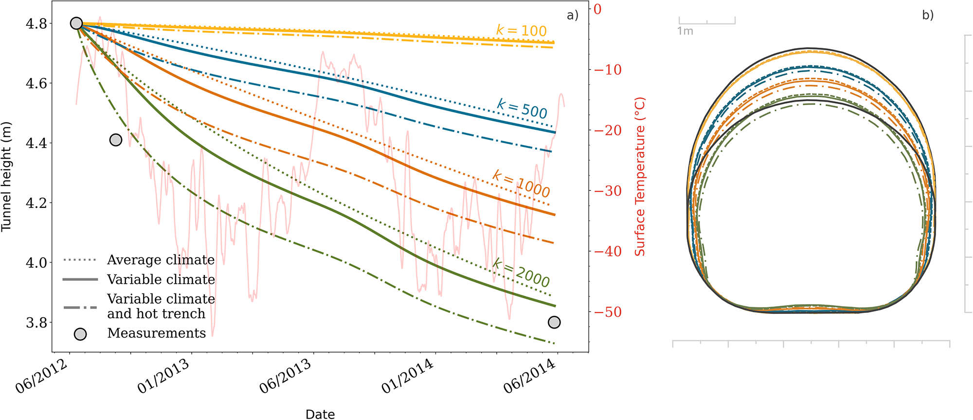
The NEGIS is a coherent structure of fast ice flow, initiating less than  $150\,\text{km}$ from the ice divide and extending more than $600\,\text{km}$ to the coast (Grinsted and others, Reference Grinsted2022). Elevation maps obtained from ArcticDEM (Porter and others, Reference Porter2018) show that, compared to average surface height variations, there are relatively pronounced depressions in the shear margins of NEGIS (Fig. 8), and recent work by Hvidberg and others (Reference Hvidberg2020) has verified the depths of the troughs (depressions) in ArcticDEM using GPS stakes.
ArcticDEM surface topography upstream of NEGIS, hillshaded using the 3D visualization software Blender. The EGRIP drill site is located at the black ball. Note that North has been rotated 135∘ clockwise to make the view of the ice-stream margin most clear, hence flow is toward the bottom part of the figure.
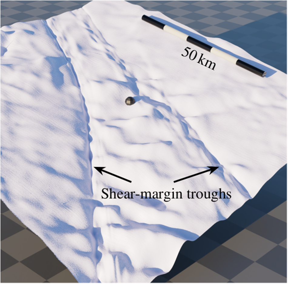
The origin of the shear margin troughs was revealed in a recent seismic survey by Riverman and others (Reference Riverman2019) (survey transect is shown in Fig. 9 as a white line, and the surface height in Fig. 10b as a blue line), finding that there is enhanced densification at the shear margins (blue contours in Fig. 10c). Oraschewski and Grinsted (Reference Oraschewski and Grinsted2022) later showed that these depressions might partly be explained by strain softening, as the horizontal velocity gradients are large there.
Satellite-derived surface velocities around EGRIP from the MEaSUREs program (Howat, Reference Howat2020) and transect (white line) of the 79 geophones used for the seismic survey performed by Riverman and others (Reference Riverman2019).
(a) Absolute value of the smoothed horizontal strain-rate components along the NEGIS seismic transect (solid lines), and the effective horizontal strain rate  ${\dot{\epsilon}}_{\mathrm{eff}}$ by Oraschewski and Grinsted (Reference Oraschewski and Grinsted2022), which includes the upstream history, too. (b) Modeled (red and yellow lines) and GPS-measured (blue line) surface elevation anomaly profile along the seismic transect (Riverman and others, Reference Riverman2019). Solid and dashed lines represent isothermal and hot shear-margin experiments, respectively. (c) Modeled BCO depth profiles (lines) plotted on top of the observed density field by Riverman and others (Reference Riverman2019). The white line shows the observed $\rho=830\,\text{kg}\,\text{m}^{-3}$ BCO depth contour, and the violet line shows the BCO depth modeled by Reference Oraschewski and GrinstedOraschewski and Grinsted (OG22). Vertical solid lines show the modeled shear-margin center points (deepest troughs), and dashed lines show the horizontal extent of the imposed $6{^\circ}\text{C}$ temperature anomaly in the shear margins. The along flow dimension, x, is pointing out of the plane.
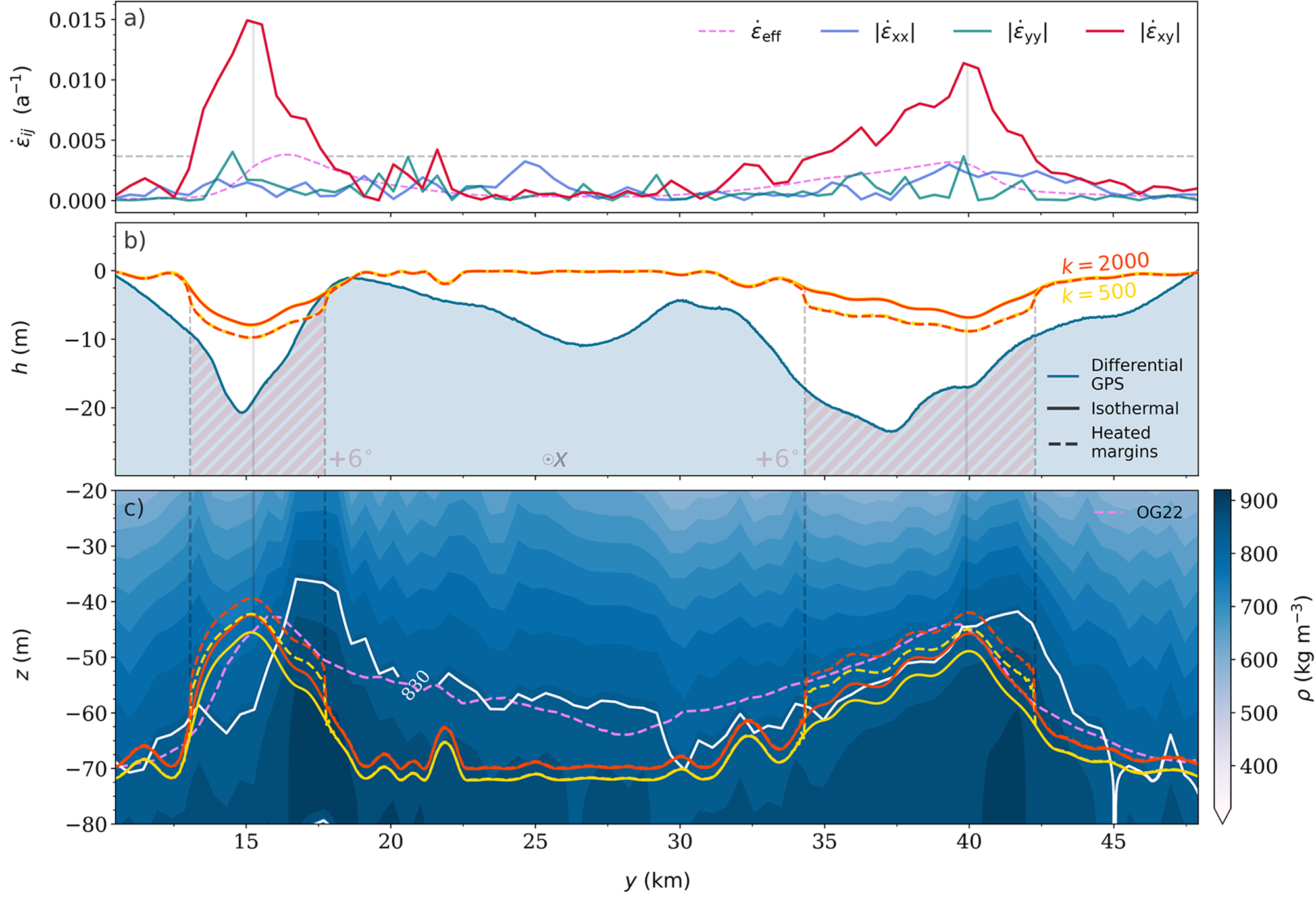
Reproducing the shear-margin troughs in a model of Riverman’s transect therefore makes for a good test case of the GM97 rheology (which accounts for strain softening) and potentially allows for another independent way to estimate the best value of k. In addition to the observed shear-margin troughs (blue line in Fig. 10b), we also include the observed BCO depth (i.e. depth at which  $\rho=830\,\text{kg}\,\text{m}^{-3}$) as a calibration target (white line in Fig. 10c). Note that the ability to model BCO depths might be less sensitive to the value of k and more sensitive to the functional forms of a and b (densities are large at the BCO).
We model the transect using a setup that combines the approaches from both the one-dimensional firn column and NEEM trench models. The yz domain considered is  $L=47.5\,\text{km}$ wide and $H=200\,\text{m}$ tall, including a $5\,\text{km}$ buffer on both lateral sides to prevent the boundaries from affecting the interior solution (extension not shown in the figures). The boundary conditions are free-slip on the left and right boundary:
 \begin{equation}
u_y(y=0,z) = 0,
\end{equation}
\begin{equation}
u_y(y=0,z) = 0,
\end{equation} \begin{equation}
u_y(y=L,z) = 0,
\end{equation}
\begin{equation}
u_y(y=L,z) = 0,
\end{equation}whereas a non-zero mass flux is imposed on the bottom boundary that balances the surface-integrated mass flux:
 \begin{equation}
u_z(y,z=-H) = -\dot{a} \frac{\rho_{\mathrm{sfc}}}{\rho_{\mathrm{ice}}}.
\end{equation}
\begin{equation}
u_z(y,z=-H) = -\dot{a} \frac{\rho_{\mathrm{sfc}}}{\rho_{\mathrm{ice}}}.
\end{equation}Here, H is taken large enough to ensure that the density at the bottom boundary is that of pure ice. The density field is subject only to the surface boundary condition
 \begin{equation}
\rho(y,z=0) = \rho_{\mathrm{sfc}}.
\end{equation}
\begin{equation}
\rho(y,z=0) = \rho_{\mathrm{sfc}}.
\end{equation} The surface density is considered to be  $\rho_{\mathrm{sfc}}=343$ kg m−3 (average of the top 2 m of firn, Schaller and others (Reference Schaller, Freitag, Kipfstuhl, Laepple, Steen-Larsen and Eisen2016)) while the accumulation rate is taken to be uniform across the transect for simplicity, $\dot{a}=130$ kg m−2 yr−1 (Karlsson and others, Reference Karlsson2020), despite it may be up to a $20\%$ higher in the shear margins due to drift snow trapped by the troughs (Riverman and others, Reference Riverman2019). The surface height profile h(y) was updated following the usual kinematic equation for free surface evolution:
 \begin{equation}
\frac{\partial h}{\partial t}= \dot{a} + u^{\text{(s)}}_z-u^{\text{(s)}}_y\frac{\partial h}{\partial y},
\end{equation}
\begin{equation}
\frac{\partial h}{\partial t}= \dot{a} + u^{\text{(s)}}_z-u^{\text{(s)}}_y\frac{\partial h}{\partial y},
\end{equation} where  $\dot{a}$ is the surface accumulation rate, and $u^{(\mathrm{s})}_y$ and $u^{(\mathrm{s})}_z$ are the surface velocity components in the yz model domain. When re-meshing after updating the surface boundary, the density field was linearly interpolated onto the new mesh.
In the absence of any horizontal variation in boundary conditions and initial state, the density field would remain horizontally homogeneous in time (the column would evolve solely due to gravitational compaction). However, additional out-of-plane strain rate components play an important role in the NEGIS transect: the shear margins experience large horizontal x–y shear (red line in Fig. 10a) that can cause significant strain softening, and the trunk might experience a slight extending flow (if any) in the along-flow x-direction (blue line in Fig. 10a). We therefore superimpose the observed  $\dot{\epsilon}_{xy}(y)$ profile on our y–z model domain by assuming it to be depth invariant, while neglecting $\dot{\epsilon}_{xx}$ and $\dot{\epsilon}_{yy}$ as they are comparatively small. All strain rates were calculated based on satellite-derived velocities from the MEaSUREs program (Howat, Reference Howat2020) and slightly smoothed to avoid numerical instabilities. Finally, lacking information about the $\dot{\epsilon}_{xz}$ shear component, we set it to zero following the shallow shelf approximation, commonly used to model ice stream flow.
The effect of the out-of-model-plane component  $\dot{\epsilon}_{xy}$ on strain softening is included by extending the strain rate invariants that enter the effective viscosity, $\dot{\epsilon}_{\mathrm{E}}$, according to (to be consistent with) their three-dimensional definitions:
 \begin{equation}
\mathrm{tr}(\dot{\boldsymbol{\epsilon}}) = \mathrm{tr}(\dot{\boldsymbol{\epsilon}}_{\text{2D}}),
\end{equation}
\begin{equation}
\mathrm{tr}(\dot{\boldsymbol{\epsilon}}) = \mathrm{tr}(\dot{\boldsymbol{\epsilon}}_{\text{2D}}),
\end{equation} \begin{equation}
\dot{\boldsymbol{\epsilon}} : \dot{\boldsymbol{\epsilon}} = \dot{\boldsymbol{\epsilon}}_{\text{2D}} : \dot{\boldsymbol{\epsilon}}_{\text{2D}} + 2 \dot{\epsilon}_{xy}^2,
\end{equation}
\begin{equation}
\dot{\boldsymbol{\epsilon}} : \dot{\boldsymbol{\epsilon}} = \dot{\boldsymbol{\epsilon}}_{\text{2D}} : \dot{\boldsymbol{\epsilon}}_{\text{2D}} + 2 \dot{\epsilon}_{xy}^2,
\end{equation} where  $\boldsymbol{\dot{\epsilon}}_\text{2D}$ is the two-dimensional strain rate tensor in our yz model.
For the temperature field across the transect, we consider two different scenarios. In the first scenario, we assume a uniform temperature of  $T=-28{^\circ}\text{C}$ (and thus a uniform flow-rate factor) (Table 1). In the second scenario, we impose a $6{^\circ}\text{C}$ elevated temperature in the ice-stream shear margins as reported by Holschuh and others (Reference Holschuh, Lilien and Christianson2019) (high-end estimate, could be lower), postulated to be caused by strain heating. Since ice is a good thermal insulator, the $6{^\circ}\text{C}$ anomaly is specified as an abrupt but depth-constant step function crossing into the shear margins. Although adding a thermal coupling to this problem as well (i.e. evolving the temperature field) would increase the physical realism, the out-of-plane heat flow is poorly known, making the thermal problem not well-posed. On the other hand, by imposing the above-mentioned steady temperature fields, the effect of dynamic strain softening (due to nonlinear viscosity) is made clearer, as its effect can be understood in isolation.
For brevity, we report only on four transient simulations that are chosen to be representative of our results: k = 500 and k = 2000 for each of the two temperature field scenarios. Here, we consider the simulation to have reached a steady-state solution once the surface elevation changes by less than  $0.02\,\text{m}$ per year (which, with a timestep of 1.25 a, takes around several hundred iterations to achieve). Also, since the different model simulations result in firn slabs of different thicknesses, when plotting, we offset the model frames to ensure a common surface elevation, allowing for an easier comparison with the observed elevation profile. The steady-state surface elevations and BCO depths modeled are plotted in Fig 10b, c, respectively, along with the observed profiles.
Overall, we find that the model (red and yellow lines) predicts higher rates of densification in the shear margins, where the shallowest part of the modeled firn columns are found to align with the maximum in horizontal shear strain rates. As expected, increasing k or shear-margin temperatures results in a softer firn that shortens the shear-margin firn column (raises the BCO depth).
Comparing the surface elevation profiles (Fig. 10b), the model can at best explain half the depth of the shear-margin troughs, with the hot shear-margin scenario predicting the deepest troughs. Once a common vertical offset is set, the predicted surface elevation profiles are found to be practically identical regardless of k. The model cannot capture the central depression, observed around  $y\simeq 27.5\,\text{km}$, which appears not to be related to strain-softening effects since both $\dot{\epsilon}_{xy}$ and $\dot{\epsilon}_{xx}$ profiles are negligible there. In addition, we find a horizontal mismatch between the modeled trough locations and observations.
The predicted BCO depths, on the other hand, seem to match observations better, with the k = 2000 heated margin scenario being better able to reproduce the observed BCO profile. However, independent of k, the measured depth minima of the BCO depth are, like the troughs, horizontally offset compared to the local  $\dot{\epsilon}_{xy}$ maxima. Further, the modeled BCO depth contour decreases more quickly than observations in the left shear margin.
4. Discussion
4.1. Reproducing Greenlandic ice cores
Our model results for the six Greenlandic firn cores suggest that the GM97 rheology is best evaluated by separately considering two different density ranges (depth ranges) of the modeled firn column.
For  ${\hat{\rho}} \gt 0.8$, the model is unable to closely reproduce the observed density profiles regardless of the value of k and generally underestimates the density for a given depth (see, e.g. Fig. 4 below $-50\,\text{m}$). At these higher densities, the coefficient functions are defined following the analytical model by Duva and Crow (Reference Duva and Crow1994), which the authors remarked might overestimate the densification rate for uniaxial compression but underestimate when the stress state is close to hydrostatic. On one hand, their caveats are insufficient for explaining our underestimated densification rate since our model assumes uniaxial compression, but, on the other hand, could be a possible explanation since incompressibility is indeed approached at the bottom part of the firn column.
However, for k = 10, the predicted density profiles are in better agreement with the deeper observations (see, e.g. Fig. 4 for  ${\hat{\rho}} \gt 0.8$), suggesting a possible mismatch between the optimal value of k needed for reproducing the near-surface and near-BCO parts of the firn column. This, we speculate in turn, might suggest some kind of inconsistency in either $a_0,b_0$ or $a_1,b_1$.
For  ${\hat{\rho}} \lt 0.8$, the model performance is very sensitive to the choice of k, which affects the decrease in compressibility with increasing density (see Methods section). There, we are generally able to find good fits of k for reproducing the Greenlandic cores. There is, however, a risk of overfitting since noise and uncertainties in the measurements ultimately affect the spread in best-fit estimates of k, so this sort of analysis can only be taken so far. As shown in Fig. 4, the lower-density observations always fall between the profiles modeled for k = 100 and k = 1000, implying that the best value is somewhere in between. Indeed, this is a general tendency across all six firn cores, suggesting that k might be somewhat less than the canonical value of $k\simeq 1000$. We note that this discrepancy could, in part, be explained by the calibration of a and b (Gagliardini and Meyssonnier, Reference Gagliardini and Meyssonnier1997, Zwinger and others, Reference Zwinger, Greve, Gagliardini, Shiraiwa and Lyly2007) being based on the cold room experiments by Langway (Reference Langway1970). Due to obvious practical limitations, these mechanical tests cannot replicate the slow in situ densification process, so they are performed at higher temperatures and stresses. While their calibration of k worked well for the density profile that the rheology was validated against, it is not surprising that different values of k might provide better fits at other sites.
The only site-specific parameters in our firn model are the depth-average temperature, surface density and accumulation rate, which means that further local characteristics that affect the densification are neglected (some of which are captured to some extent in other models—e.g. grain-size effects; Kingslake and others (Reference Kingslake, Skarbek, Case and McCarthy2022)). Within our simple one-dimensional firn model, it is therefore not surprising that these few site-specific parameters are insufficient for capturing the full diversity of the densification process. On that note, it is also possible that the coefficient functions a and b have some dependencies not considered in the model, especially temperature (see the discussion of the NEEM tunnel experiments below). Finally, uncertainties in the imposed, observed surface densities affect not only the near-surface solution but eventually also the compressibility of the whole firn column by virtue of  $a(\rho(z))$ and $b(\rho(z))$, underlining the importance of accurate surface density measurements for future studies.
4.1.1. Steady-state assumption
The steady-state density profiles calculated here do not, by definition, include effects from seasonal variations in temperature (or melt, for that matter). Given the exponential flow rate factor A(T), our model might therefore be underestimating the rate of densification due to warm temperature anomalies softening the firn more than equivalent cold anomalies would stiffen it. Similar asymmetric responses to temperature have already been reported in other cases (e.g. firn air content; Thompson-Munson and others (Reference Thompson-Munson, Wever, Stevens, Lenaerts and Medley2023)) and, as found in the comparison between the average and variable climate scenarios in Fig. 7, this asymmetry also affects the firn column height and density profile. A more realistic model setup might therefore result in a smaller k, since the inferred k for a given temperature profile would, in our current model setup, have to compensate for the fact that A(T) should have been (somewhat) larger.
Another factor disregarded here is the present-day superimposed warming trend, which implies that the near-surface firn temperatures are hotter than the depth-averaged temperature. Similarly to the effect of seasonal variation, a more realistic model setup that could account for thermal heterogeneities might therefore produce lower estimates of k. The depth-averaged thermal profiles used here might therefore also explain some of the spread in k estimated between sites since each core is likely to be affected differently due to different extraction dates and the climate experienced.
4.1.2. Is k universal?
With all of the above caveats taken into account, our RMSE analysis (Fig. 3) suggests that there is no optimal value of k, universally applicable to all sites. Nonetheless, our results of one-dimensional firn compaction indicate that, if a single value of k is to be used, a value in the range of 100–400 is probably better than the canonical value of k = 1000. If the sample size of relevant firn cores could be expanded in future work, a more accurate value of k might be sought with higher confidence by using a global RMSE metric (combined RMSE across all cores for a given k; not attempted here), which would also allow for more robust uncertainty quantification.
Addressing the mentioned model shortcomings might lead to improved misfits and thus, potentially, a better ability to determine whether a universal value of k exists. But given the misfits found in the deeper part of the firn columns (e.g.  ${\hat{\rho}} \gt 0.8$ in Fig. 4 for Site 2)—where much smaller values of k are needed to reproduce observed densities—our results suggest that more work is equally needed to understand the limitations of the canonical coefficient functions a and b.
Taken together, we therefore argue that the benefit of the GM97 rheology is (as of now) not to provide a new tool for altimetry corrections but rather its ability to seamlessly represent multidimensional firn compaction in large-scale transient problems.
4.2. Trench collapse at NEEM
The results from the NEEM trench simulations do not agree with our one-dimensional firn compaction results. Overall, setting  $k\simeq 2000$ gives the best agreement with the observed trench deformation, which is twice the canonical value and ten times that needed to minimize the RMSE of the NEEM density profile (Fig. 3). This is somewhat surprising since such a magnitude of k causes a significant overestimation of the near-surface densification rate in our one-dimensional model above (taking the above model caveats into account), and we have no reason to believe that a and b should not apply to both one- and two-dimensional problems. Although it is possible that calibrating against surface experiments is not necessarily comparable to the above full-column calibrations, the disagreement between estimates of k suggests that either the experimental conditions are not realistic enough, they have changed significantly since the formation of the firn column (e.g. due to the warming climate) or the model fails to properly reproduce some important aspect of the densification process. Combining all the specifications of the technical report (Steffensen, Reference Steffensen2014) with the surface measurements made by affiliated projects at NEEM, we believe that the present experimental conditions are as detailed as they can practically be for this experiment, but several sources of uncertainty are still relevant to consider.
First, the hot trench simulations clearly show that the choice of initial temperature field is a key factor in this problem. Despite all scenarios resulting in a progressively reduced rate of collapse as time passes, the observed pronounced initial collapse rate (grey dots in Fig. 7) is best explained if a hotter initial trench is taken into account. However, by setting k sufficiently large, the observed initial collapse rate can also be roughly reproduced. But that affects the final tunnel height, making it considerably shorter than observed because the firn is, in effect, made too compressible. The only way to reproduce both the transient change in tunnel height and its final height is therefore by an appropriate choice of both k and initial thermal state. If it is possible to repeat this experiment in the future, we thus suggest that the temperature field also be well documented to reduce uncertainties in the model initial state.
Second, unusually high atmospheric temperatures, recorded during the first summer of the experiment, reached six positive temperature days and caused extraordinary melt events that were observed covering the tunnel ceiling in blue refrozen meltwater patches (Steffensen, Reference Steffensen2014). The tunnel evolution was surely impacted by the presence of this percolating liquid water, which, apart from perturbing the temperature and density fields, has been observed to accelerate grain growth and affect densification rates (Brun, Reference Brun1989, Sturm and Holmgren, Reference Sturm and Holmgren1998, Mizukami and Perica, Reference Mizukami and Perica2008). This might have contributed to the observed initial collapse rate, and Reference SteffensenSteffensen believed that it had perturbed the structural rigidity of the tunnel (Steffensen, Reference Steffensen2014). Additional uncertainties that may have favored the exceptionally large initial deformation rate could be the effect of nearby tunnels and structures or the wind-enhanced accumulation due to the proximity to the main camp dome (not considered here).
We emphasize that the large best-fit value of  $k\simeq 2000$ is not a consequence of neglecting the recent surface warming trend; setting the depth-average firn temperature as the surface boundary condition results in a tunnel evolution that is almost identical to the average current-climate experiments in Fig. 7 (results not shown). This means that, regardless of whether the model is forced with present-day temperatures or not (the impact of any recent trend is not significant in the depth-averaged temperature yet), a larger value around $k\simeq 2000$ is required to fit the observed rate of collapse.
Finally, a source of uncertainty is of course the model uncertainty. For example, it is possible that the coefficient functions a and b also depend on temperature, although the GM97 rheology assumes that A(T) captures the effect of temperature alone. If so, the optimal value of k would also have to account for some sort of effective contribution/adjustment due to temperature. As long as the climatic conditions are stable, this contribution would likely only vary between sites, but changes in thermal conditions (such as the average surface temperature or amplitude of the seasonal variations) could, in this way, also contribute to model uncertainty.
Taken together, we argue that the conditions considered in our simulation might not have captured those at NEEM during 2012–14 sufficiently well, and thus the best fit  $k\simeq 2000$ inferred from this test is subject to considerable uncertainty. Our results also underline the impact that initialization and boundary conditions can have on these kinds of model predictions, along with processes unaccounted for such as surface melting, which complicate model calibration and validation attempts. Nonetheless, our sensitivity tests and experiments are sufficient to provide some qualitative insight into the structural characteristics of these tunnels. While not shown here, this also includes how to maximize the lifetime of subsurface tunnels, which we find requires a carefully selected combination of initial tunnel shape and the cross-sectional profile of backfilled snow. This line of modeling could be relevant for the future development and design of trenches, whether for ice core drilling projects or as storage facilities (e.g. Brondex and others, Reference Brondex, Gagliardini, Gillet-Chaulet and Chekki2020).
4.3. NEGIS shear margin troughs
We find that our NEGIS cross-section model is partly able to reproduce the faster densification observed at the shear margins near EGRIP, resulting in shallower firn columns. Despite the idealized nature of our model and boundary conditions (elaborated on below), we believe that our results are sufficiently convincing to support the hypothesis that the deep troughs are partly due to nonlinear-viscous firn softening/compaction, resulting from significant shear-margin strain rates. There are, however, some differences compared to observations that suggest important model shortcomings but also highlight a path forward for future studies of firn densification over ice streams.
In order to characterize the model mismatch with observations more carefully, we include for comparison two useful results from Oraschewski and Grinsted (Reference Oraschewski and Grinsted2022): (i) the effective horizontal strain rate experienced by the firn column throughout its formation ( ${\dot{\epsilon}}_{\mathrm{eff}} = \sqrt{\dot{\boldsymbol{\epsilon}}:\dot{\boldsymbol{\epsilon}}/2}$ integrated along upstream flow lines; dashed violet line in Fig. 10a) and (ii) the BCO depth contour modeled by Oraschewski and Grinsted (Reference Oraschewski and Grinsted2022) using their strain-rate-scale-factor model that relies on ${\dot{\epsilon}}_{\mathrm{eff}}$ (dashed violet line in Fig. 10c).
4.3.1. Trough depths
The predicted elevation profiles appear to be insensitive to the value of k, but this is not the case for two subtle reasons. First, Fig. 10b shows the surface height after setting a common surface reference to allow easy comparison with observations; that way, the  $\sim 3\,\text{m}$ difference in surface heights between experiments with different k is manifested instead at depth (e.g. the BCO depths are shifted accordingly). Second, sensitivity tests indicate that the difference in modeled surface height of steady-state firn columns, for different choices of k, does not change as the superimposed shear strain rate increases (data not shown). Although the predicted densification rates are affected by a superimposed strain rate (rendering the firn column shallower in the shear margin), the difference between surface heights for different k thus remains independent along the transect. Hence, while the height of the firn column is reduced with increasing k, the depth of the surface trough is independent of k, leaving the shear-margin surface troughs not useful for assessing/calibrating k.
Regarding the effect of temperature, anomalies can have an important impact on densification rates, as seen in the NEEM trench model. Our experiments with  $+6{^\circ}\text{C}$ warmer shear margins soften the local firn column, significantly improving the predicted surface elevation and BCO depth profiles. However, the applied step-function temperature field is rather simplified; the transition to the maximum temperature (where shear strain rates are maximal) surely occurs more gradually. Nonetheless, our results are intended as a first-order estimate of the effect of warm shear margins that can be understood as an upper bound.
Since the mismatch between the modeled and observed surface shape is insensitive to k, and the potential effect of warmer margins is relatively limited, the remaining  $\sim 10\,\text{m}$ discrepancy in trough depths might, in part, be due to the horizontal variation of the accumulation neglected in this study. Even if such conditions were well known, the modeled cross-section should not be expected to reproduce all observed density contours exactly since upstream flow corrections are not accounted for; that is, firn parcel trajectories might in reality not be vertical as modeled but could enter the domain obliquely.
We also speculate that the empirically proposed parts of the coefficient functions a and b, relevant for low-density firn, might be too crude to capture the densification process in more exotic strain rate regimes, such as ice stream shear margins. The main reason being that the real strain rate history, experienced by the firn column, is probably closer to  ${\dot{\epsilon}}_{\mathrm{eff}}$ (dashed violet line in Fig. 10a), which is supposed to also include the upstream past in an effective sense. Insofar as this measure is accurate, it is much smaller than the typical shear-margin strain rates used here, and therefore the magnitude of the resulting troughs would be only half as deep for a given k (not shown). Given the already shallow depressions, this would make the origin of the shear margin troughs even harder to explain.
We mention that the central depression is ignored here, as it is possibly caused by ice flow effects, resulting from a combination of upstream flow effects and interactions with the subglacial environment (Christianson and others, Reference Christianson2014, Riverman and others, Reference Riverman2019, Hvidberg and others, Reference Hvidberg2020). Note that this irregular wavy structure is present throughout the trunk of the ice stream (Fig. 8). A more realistic, three-dimensional ice stream model of the entire ice–firn column might lead to a better understanding of how the broader ice-flow setting could induce this wavy surface topography (left for future research). The same applies to understanding to what extent the effective strain rate  ${\dot{\epsilon}}_{\mathrm{eff}}$ is a useful measure (i.e. can account for upstream effects in an integrated sense), which could be validated, or at least better understood, if calculated in a three-dimensional firn model of the ice stream.
4.3.2. Horizontal offsets
Another discrepancy with observations is that the modeled firn columns are most shallow exactly where  $|{\dot{\epsilon}_{xy}}|$ peaks, while observed shear-margin surface depressions (measured by differential GPS) and the BCO depth minima are shifted by $\sim 2.5$– $5\,\text{km}$ (Fig. 10b, c). In contrast, this shift is less apparent in the work by Oraschewski and Grinsted (Reference Oraschewski and Grinsted2022), likely a consequence of having used ${\dot{\epsilon}}_{\mathrm{eff}}$ as the forcing strain rates, which follows the observed BCO depth profile closer than the local strain-rate profile used here. This suggests that some upstream correction to our superimposed shear strain rate field might reduce the horizontal offset between modeled and observed BCO depths. But the same correction does not necessarily apply to all layers (especially to those closer to the surface), since the age of the parcel and, thus, the upstream trajectories, are different (shorter). If taken into account (assuming the superimposed shear strain rate is indeed depth constant), it is possible that offsets between the modeled and observed trough positions and BCO depths might be explained.
4.3.3. BCO depths
Overall, the predicted BCO depth profiles match observations better than the surface elevation, capturing the most defining features reasonably well. Unfortunately, these do not help much in assessing the optimal value of k for the same reason that the shear margin troughs are not useful; the sensitivity of the modeled BCO depth profile to k is very small compared to the effect of superimposed shear strain rates (not to mention the uncertainties in the seismically inferred BCO depth contour by Riverman and others (Reference Riverman2019)).
One striking mismatch is the missing ‘tail’ of the left-hand side BCO peak, contrary to the right-hand side; modeled BCO depths drop off much faster toward interior values than observed. The profile of  ${\dot{\epsilon}}_{\mathrm{eff}}$ (violet dashed line in Fig. 10a) does not necessarily suggest that upstream effects can explain this skewed BCO depth contour, at least given the present-day velocity map used here. Grinsted and others (Reference Grinsted2022) recently reported an observed outward acceleration of the shear margins, which is strongest on the southern shear margin (left-hand side in Fig. 10). The northern shear margin (right-hand side in Fig. 10) has a somewhat double margin structure (Jansen and others, Reference Jansen2024) that apparently does not seem to affect the predicted BCO depth, and a recent radar survey (Nymand and others, Reference Nymand2024) found that the crystal fabric there (unlike the southern shear margin) does not match modeled fabrics well, suggesting the northern shear margin might be more dynamic. Therefore, if the outward acceleration of the southern shear margin is indeed related to the ‘tail’ misfit, it is not entirely clear why the modeled BCO depth in the northern shear margin fits observations better.
Our simulations rely on present-day strain rates that are almost four times bigger than the flow-line integrated effective strain rate  ${\dot{\epsilon}}_{\mathrm{eff}}$. If superimposing ${\dot{\epsilon}}_{\mathrm{eff}}$ is more accurate than using $\dot{\epsilon}_{xy}$ as done here, the firn column height predicted by the GM97 rheology at the shear margins would be notably smaller than observed (similar in magnitude to our results at $y\simeq 22\,\text{km}$). Since choosing a different k cannot improve the misfit (cf. above discussion), this could suggest that the definition of the coefficient functions a and b would be worth revisiting.
4.3.4. Implications for ice-core proxies
An accurate model for predicting how strain softening can cause shallower firn columns would be a useful tool to help the interpretation of some ice core proxies. In the case of gas measurements, for example, our results agree with Oraschewski and Grinsted (Reference Oraschewski and Grinsted2022), suggesting that in the shear margins of NEGIS, BCO is reached up to ∼ 200 a earlier than in the center of the ice stream where it takes around 400 a (estimated as the time taken for firn parcels to reach BCO density, starting from the surface and subject to the modeled steady-state velocity field). As a consequence, the age difference between the gas and surrounding ice, Δage, is smaller, which should be accounted if ice cores were to be drilled there; conversely, this could be a reason for drilling ice cores in ice stream shear margins (higher gas age resolution). What this means for the Δage profile in the EGRIP ice core is unclear, but present-day surface velocities suggest that firn parcels ending up in the EGRIP core did not pass through the ice stream shear margins (Hvidberg and others, Reference Hvidberg2020).
5. Conclusion
In this paper, we applied the firn rheology by Gagliardini and Meyssonnier (Reference Gagliardini and Meyssonnier1997) (GM97) to several present-day firn densification problems in Greenland using the finite element method. Unlike many existing one-dimensional firn models, the GM97 rheology can account for arbitrary, three-dimensional stress configurations (including the effect of strain softening), and seamlessly represents both firn and ice in a single continuum description. This makes GM97 a promising rheology that enables the study of complex firn densification scenarios, but its calibration and general performance arguably require more testing, such as on a wider range of conditions and flow settings.
With that focus, we revisited the canonical compressibility and viscosity functions of the rheology, proposed by Zwinger and others (Reference Zwinger, Greve, Gagliardini, Shiraiwa and Lyly2007), by extending their calibration to include five additional Greenlandic firn cores. While the model is able to reasonably fit all the density profiles by varying the free calibration parameter, k, between 100 and 500 (lower than the canonical  $k\simeq 1000$ proposed by Zwinger and others (Reference Zwinger, Greve, Gagliardini, Shiraiwa and Lyly2007)), we find that no single calibration is applicable to all six cores. We suggest that more work might be needed to determine whether better-suited functional forms exist for the compressibility and viscosity of firn, although climate-induced variations on firn mechanical properties were not considered due to steady-state assumptions.
Seeking another independent way to validate the GM97 calibration, we attempted to reproduce the collapse of a firn tunnel, constructed at NEEM ice core site, Greenland. While the GM97 rheology was found to be well-suited for simulating the transient deformation of the tunnel geometry, the dependence of densification rate on density was found to be very sensitive to the exact value of k. Combined with other unknowns related to the thermal forcing history and the presence of melt water, we conclude that the experimental conditions at NEEM were probably insufficiently documented to allow us to prescribe realistic model boundary conditions. We therefore have less confidence in the resulting best-fit (calibration) of  $k\simeq 2000$.
Finally, we constructed a cross-section model of the NEGIS to assess whether the higher rate of densification, observed in the ice stream shear margins, might be explained by increased strain softening due to large horizontal shearing. Supporting this hypothesis, we found that modeled firn columns in the shear margins are indeed shallower when accounting for the observed horizontal shear and elevated temperatures. Even though upstream and depth corrections are probably needed to fully understand the mismatch between model and observations, and that modeled surface trough depths can account for only half the observed depths, other important features such as the BCO depth are better reproduced. The NEGIS experiment was not found useful to further constrain the compressibility and viscosity functions of the GM97 rheology due to the depths of the resulting surface depression and BCO perturbation not being sufficiently sensitive to k.
In summary, we demonstrated that the GM97 rheology is useful for simulating firn densification under a diverse set of stress/strain scenarios, making it relevant for future use cases such as modeling horizontal firn density variations over ice sheets for mass-loss estimates or estimating ice–gas age differences for ice-core proxy interpretations. However, our work also suggests that it would be worth revisiting the compressibility and viscosity functions of the GM97 rheology, such as validating/calibrating them in more carefully constructed lab experiments to determine their density and temperature dependencies in greater detail.
Data availability statement
The codes used to produce the model runs and plots of this work can be found in the following repository: https://github.com/jonarri/JOG_FirnDensificationIn2D_GM97.
Acknowledgements
We wish to thank Editor Alan Rempel, Max Brils and an anonymous reviewer for providing comments that greatly improved the structure of our manuscript and the numerical experiments considered.
Author contributions
All authors contributed to the methodology, based on initial ideas by NMR, AG and CSH. JAI and LLG wrote all model code and performed all simulations under the supervision of NMR. JAI, LLG and NMR wrote the first draft. All authors contributed to the final manuscript.
Funding statement
The research leading to these results has received funding from the Novo Nordisk Foundation, grant no. NNF23OC0081251, the Independent Research Fund Denmark (DFF), grant no. 2032-00364B, the Villum Foundation, grants no. 23261 and 16572 and by ref. CEX2021-001201-M funded by MCIN/AEI/ 10.13039/ 501100011033. JAI benefits from a predoctoral grant from the Basque Government (PRE_2023_1_0131).
EGRIP is directed and organized by the Centre for Ice and Climate at the Niels Bohr Institute, University of Copenhagen. It is supported by funding agencies and institutions in Denmark (A. P. Møller Foundation, University of Copenhagen), USA (US National Science Foundation, Office of Polar Programs), Germany (Alfred Wegener Institute, Helmholtz Centre for Polar and Marine Research), Japan (National Institute of Polar Research and Arctic Challenge for Sustainability), Norway (University of Bergen and Trond Mohn Foundation), Switzerland (Swiss National Science Foundation), France (French Polar Institute Paul-Emile Victor, Institute for Geosciences and Environmental research), Canada (University of Manitoba) and China (Chinese Academy of Sciences and Beijing Normal University).
Competing interests
The authors declare that they have no competing interests.
Appendix A: Weak forms
The weak or variational forms solved in FEniCS are obtained by multiplying the respective PDEs with a weight function, w (or w if vectorial), and integrating over all space. Terms involving second-order derivatives are integrated by parts the usual way to reduce them to first-order derivatives at the expense of adding boundary integrals. In the following, Ω and Γ will represent the volume and the bounding surface of the model domain, respectively (or in two dimensions, area and bounding line).
For mass conservation, the weak form is
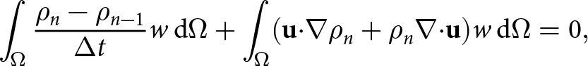 \begin{align}
\int_{\Omega} \frac{\rho_n-\rho_{n-1}}{\Delta t} w\,\mathrm{d}{\Omega}
+ \int_{\Omega} ({\mathbf{u}}{\boldsymbol\cdot}{\boldsymbol\nabla}\rho_n + \rho_n{\boldsymbol\nabla}{\boldsymbol\cdot}{\mathbf{u}})w\,\mathrm{d}{\Omega} = 0,
\end{align}
\begin{align}
\int_{\Omega} \frac{\rho_n-\rho_{n-1}}{\Delta t} w\,\mathrm{d}{\Omega}
+ \int_{\Omega} ({\mathbf{u}}{\boldsymbol\cdot}{\boldsymbol\nabla}\rho_n + \rho_n{\boldsymbol\nabla}{\boldsymbol\cdot}{\mathbf{u}})w\,\mathrm{d}{\Omega} = 0,
\end{align}which discretizes the time derivative using an implicit Euler scheme, and subscripts n and n − 1 refer to the solution at the new and previous time step, respectively.
The free surface evolution is solved in a similar way and has the weak form
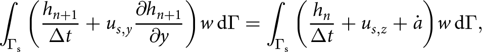 \begin{equation}
\int_{\Gamma_\mathrm{s}} \bigg(\frac{h_{n+1}}{\Delta t} + u_{s,y} \frac{\partial h_{n+1}}{\partial y}\bigg) w\, \mathrm{d}{\Gamma}
=\int_{\Gamma_\mathrm{s}} \bigg(\frac{h_{n}}{\Delta t} + u_{s,z}+\dot{a}\bigg) w\, \mathrm{d}{\Gamma},
\end{equation}
\begin{equation}
\int_{\Gamma_\mathrm{s}} \bigg(\frac{h_{n+1}}{\Delta t} + u_{s,y} \frac{\partial h_{n+1}}{\partial y}\bigg) w\, \mathrm{d}{\Gamma}
=\int_{\Gamma_\mathrm{s}} \bigg(\frac{h_{n}}{\Delta t} + u_{s,z}+\dot{a}\bigg) w\, \mathrm{d}{\Gamma},
\end{equation}where  $\mathrm{d}{\Gamma}$ is a line element along the surface segment of the boundary, $\Gamma_\mathrm{s}$.
The weak form of the momentum balance is
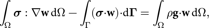 \begin{align}
\int_{\Omega} \boldsymbol{\sigma} : {\boldsymbol\nabla} {\mathbf{w}} \, \mathrm{d}{\Omega}
- \int_{\Gamma} (\boldsymbol{\sigma}{\boldsymbol\cdot}{\mathbf{w}}){\boldsymbol\cdot} \mathrm{d}{\boldsymbol{\Gamma}}
= \int_{\Omega} \rho {\mathbf{g}}{\boldsymbol\cdot}{\mathbf{w}}\, \mathrm{d}{\Omega},
\end{align}
\begin{align}
\int_{\Omega} \boldsymbol{\sigma} : {\boldsymbol\nabla} {\mathbf{w}} \, \mathrm{d}{\Omega}
- \int_{\Gamma} (\boldsymbol{\sigma}{\boldsymbol\cdot}{\mathbf{w}}){\boldsymbol\cdot} \mathrm{d}{\boldsymbol{\Gamma}}
= \int_{\Omega} \rho {\mathbf{g}}{\boldsymbol\cdot}{\mathbf{w}}\, \mathrm{d}{\Omega},
\end{align}where the middle term is the boundary traction integral that vanishes in the problems considered in the main text due to periodic boundaries or specified Dirichlet (velocity) boundary conditions.
Finally, the weak form of the temperature equation is
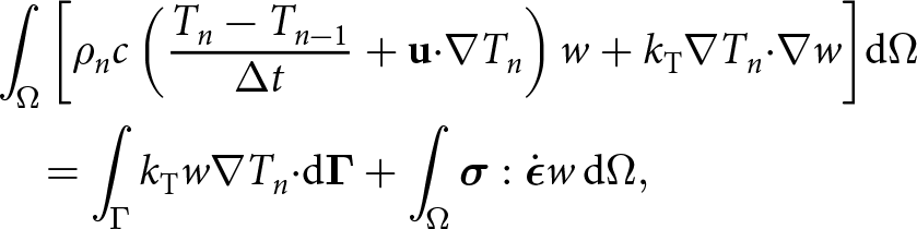 \begin{align}
&\int_{\Omega} \bigg[\rho_n c \left( \frac{T_n-T_{n-1}}{\Delta t} + {\mathbf{u}}{\boldsymbol\cdot}{\boldsymbol\nabla} T_n\right) w
+ {k_{\mathrm{T}}}{\boldsymbol\nabla} T_n {\boldsymbol\cdot} {\boldsymbol\nabla} w
\bigg] \mathrm{d}{\Omega} \nonumber\\
&\quad =
\int_{\Gamma} {k_{\mathrm{T}}} w {\boldsymbol\nabla} T_n {\boldsymbol\cdot} \mathrm{d}{\boldsymbol{\Gamma}}
+ \int_{\Omega} \boldsymbol{\sigma}:\dot{\boldsymbol{\epsilon}} w\, \mathrm{d}{\Omega} ,
\end{align}
\begin{align}
&\int_{\Omega} \bigg[\rho_n c \left( \frac{T_n-T_{n-1}}{\Delta t} + {\mathbf{u}}{\boldsymbol\cdot}{\boldsymbol\nabla} T_n\right) w
+ {k_{\mathrm{T}}}{\boldsymbol\nabla} T_n {\boldsymbol\cdot} {\boldsymbol\nabla} w
\bigg] \mathrm{d}{\Omega} \nonumber\\
&\quad =
\int_{\Gamma} {k_{\mathrm{T}}} w {\boldsymbol\nabla} T_n {\boldsymbol\cdot} \mathrm{d}{\boldsymbol{\Gamma}}
+ \int_{\Omega} \boldsymbol{\sigma}:\dot{\boldsymbol{\epsilon}} w\, \mathrm{d}{\Omega} ,
\end{align}where the second term on the right-hand side accounts for the energy flux through the model domain boundaries that vanishes if boundaries are periodic or Dirichlet (temperature) boundary conditions are specified. Here, the specific heat capacity is
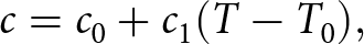 \begin{align}
c = c_0 + c_1(T-T_0),
\end{align}
\begin{align}
c = c_0 + c_1(T-T_0),
\end{align} where  $c_0=2127.5\,\text{J}\,\text{kg}^{-1}\,\text{K}^{-1}$, $c_1=7.253\,\text{J}\,\text{kg}^{-1}\,\text{K}^{-2}$ and $T_0=273.16\,\text{K}$. The thermal conductivity is
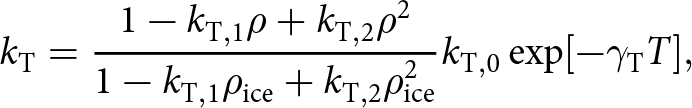 \begin{equation}k_{\mathrm T}=\frac{1-k_{\mathrm T,1}\rho+k_{\mathrm T,2}\rho^2}{1-k_{\mathrm T,1}\rho_{\mathrm{ice}}+k_{\mathrm T,2}\rho_{\mathrm{ice}}^2}k_{\mathrm T,0}\exp\lbrack-\gamma_{\mathrm T}T\rbrack,\end{equation}
where  ${k_{\mathrm{T},0}} = 9.828\,\text{W}\,\text{m}^{-1}\,\text{K}^{-1}$, ${k_{\mathrm{T},1}} = 7.3188 \times 10^{-3}\,\text{m}^{3}\,\text{kg}^{-1}$, ${k_{\mathrm{T},2}} = 2.3428 \times 10^{-5}\,\text{m}^{6}\,\text{kg}^{-2}$ and ${\gamma_{\mathrm{T}}} = 5.7 \times 10^{-3}\,\text{K}^{-1}$.
Both (A1) and (A4) use linear elements for the unknowns and weight functions (Galerkin method), whereas (A3) uses quadratic elements.
Appendix B: Rheology derivation
The rheology can be derived from plastic potential theory by assuming the effective stress,  $\sigma_{\mathrm{E}}$, depends on both the first and second stress-tensor invariants, $\mathrm{tr}(\boldsymbol{\sigma})$ and $\boldsymbol{\sigma}:\boldsymbol{\sigma}$, respectively. We follow Duva and Crow (Reference Duva and Crow1994) by writing $\sigma_{\mathrm{E}}^2$ as the particular linear combination
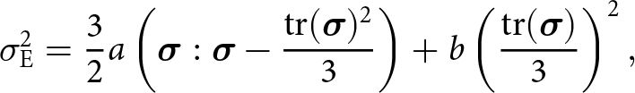 \begin{align}
\sigma_{\mathrm{E}}^2 = \frac{3}{2} a \left(\boldsymbol{\sigma}:\boldsymbol{\sigma} - \frac{\mathrm{tr}(\boldsymbol{\sigma})^2}{3}\right) + b \left(\frac{\mathrm{tr}(\boldsymbol{\sigma})}{3}\right)^2,
\end{align}
\begin{align}
\sigma_{\mathrm{E}}^2 = \frac{3}{2} a \left(\boldsymbol{\sigma}:\boldsymbol{\sigma} - \frac{\mathrm{tr}(\boldsymbol{\sigma})^2}{3}\right) + b \left(\frac{\mathrm{tr}(\boldsymbol{\sigma})}{3}\right)^2,
\end{align} where a and b are material functions of density. For conformity with Glen’s flow law in incompressible limit  $\rho\rightarrow\rho_{\mathrm{ice}}$, the relationship between the effective stress and effective strain rate, $\dot{\epsilon}_{\mathrm{E}}$, should follow the power law $\dot{\epsilon}_{\mathrm{E}}=A\sigma_{\mathrm{E}}^n$, corresponding to a Norton–Bailey creep potential. The flow rule then implies (Duva and Crow, Reference Duva and Crow1994)
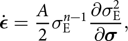 \begin{align}
\dot{\boldsymbol{\epsilon}} = \frac{A}{2} \sigma_{\mathrm{E}}^{n-1}\frac{\partial \sigma_{\mathrm{E}}^2}{\partial \boldsymbol{\sigma}},
\end{align}
\begin{align}
\dot{\boldsymbol{\epsilon}} = \frac{A}{2} \sigma_{\mathrm{E}}^{n-1}\frac{\partial \sigma_{\mathrm{E}}^2}{\partial \boldsymbol{\sigma}},
\end{align}where A is the flow-rate factor. The derivatives needed for evaluating  $\partial\sigma_{\mathrm{E}}^2/\partial\boldsymbol{\sigma}$ are $\partial(\boldsymbol{\sigma}:\boldsymbol{\sigma})/\partial\boldsymbol{\sigma} = 2 \boldsymbol{\sigma}$ and $\partial \mathrm{tr}(\boldsymbol{\sigma})^2/\partial\boldsymbol{\sigma} = 2 \mathrm{tr}(\boldsymbol{\sigma}) {\mathbf{I}}$, and the forward rheology is therefore
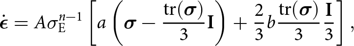 \begin{gather}
\dot{\boldsymbol{\epsilon}} = A \sigma_{\mathrm{E}}^{n-1}\left[
a \left(\boldsymbol{\sigma} - \frac{\mathrm{tr}(\boldsymbol{\sigma})}{3}{\mathbf{I}}\right) + \frac{2}{3}b \frac{\mathrm{tr}(\boldsymbol{\sigma})}{3}\frac{{\mathbf{I}}}{3}
\right],
\end{gather}
\begin{gather}
\dot{\boldsymbol{\epsilon}} = A \sigma_{\mathrm{E}}^{n-1}\left[
a \left(\boldsymbol{\sigma} - \frac{\mathrm{tr}(\boldsymbol{\sigma})}{3}{\mathbf{I}}\right) + \frac{2}{3}b \frac{\mathrm{tr}(\boldsymbol{\sigma})}{3}\frac{{\mathbf{I}}}{3}
\right],
\end{gather}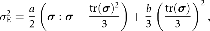 \begin{gather}
\sigma_{\mathrm{E}}^2 = \frac{a}{2}\left(\boldsymbol{\sigma}:\boldsymbol{\sigma} - \frac{\mathrm{tr}(\boldsymbol{\sigma})^2}{3}\right) + \frac{b}{3} \left(\frac{\mathrm{tr}(\boldsymbol{\sigma})}{3}\right)^2,
\end{gather}
\begin{gather}
\sigma_{\mathrm{E}}^2 = \frac{a}{2}\left(\boldsymbol{\sigma}:\boldsymbol{\sigma} - \frac{\mathrm{tr}(\boldsymbol{\sigma})^2}{3}\right) + \frac{b}{3} \left(\frac{\mathrm{tr}(\boldsymbol{\sigma})}{3}\right)^2,
\end{gather}where a factor of  $3^{(n+1)/2}/2$ has been absorbed into A. Notice that Glen’s incompressible flow law is recovered in the limit a = 1 and b = 0.
The inverse rheology can be derived by vectorizing (B3) according to
 \begin{align}
{\mathcal{V}}({\mathbf{X}}) = [X_{11},X_{21},X_{31}, X_{12},X_{22},X_{32}, X_{13},X_{23},X_{33}]^{\mathsf{T}},
\end{align}
\begin{align}
{\mathcal{V}}({\mathbf{X}}) = [X_{11},X_{21},X_{31}, X_{12},X_{22},X_{32}, X_{13},X_{23},X_{33}]^{\mathsf{T}},
\end{align}giving
 \begin{align}
{\mathcal{V}}(\dot{\boldsymbol{\epsilon}}) &= A \sigma_{\mathrm{E}}^{n-1} {\mathbf{P}} \cdot {\mathcal{V}}(\boldsymbol{\sigma}),
\end{align}
\begin{align}
{\mathcal{V}}(\dot{\boldsymbol{\epsilon}}) &= A \sigma_{\mathrm{E}}^{n-1} {\mathbf{P}} \cdot {\mathcal{V}}(\boldsymbol{\sigma}),
\end{align}where
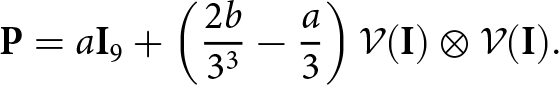 \begin{align}
{\mathbf{P}} =
a{\mathbf{I}}_9 + \left(\frac{2b}{3^3}-\frac{a}{3}\right){\mathcal{V}}({\mathbf{I}})\otimes{\mathcal{V}}({\mathbf{I}}).
\end{align}
\begin{align}
{\mathbf{P}} =
a{\mathbf{I}}_9 + \left(\frac{2b}{3^3}-\frac{a}{3}\right){\mathcal{V}}({\mathbf{I}})\otimes{\mathcal{V}}({\mathbf{I}}).
\end{align}Here, ⊗ is the generalized outer product (Kronecker product), and  $\mathrm{tr}(\boldsymbol{\sigma})={\mathbf{I}} : \boldsymbol{\sigma} = {\mathcal{V}}({\mathbf{I}}){\boldsymbol\cdot}{\mathcal{V}}(\boldsymbol{\sigma})$ was used. The inverse rheology is then given by $\boldsymbol{\sigma} = {\mathcal{V}}^{-1}({\mathbf{P}}^{-1}{\mathcal{V}}({\dot{\boldsymbol{\epsilon}}}))$, or in tensorial form as written in Equation (4).


 Open access