


Introduction
The inverse design of nanophotonic structures, obtaining a geometry for a desired photonic function (Figure 1a–b), has been a challenge for decades. When treated as a pure optimization problem, due to the highly nonlinear nature of the problem, hundreds to several thousands of iterations are required for a single design task, even with the most advanced algorithms, such as evolutionary or topology optimization algorithms (Figure 1c–d). Recently, modern machine learning algorithms, which have revolutionized a multitude of computer-assisted processes, from character and speech recognition, autonomous vehicles, and cancer diagnostics to name a few, have been applied to the inverse problem in nanophotonics and have demonstrated great promise.
Deep learning nanophotonics. (a) Interaction of light with plasmonic nanostructures. Incoming electromagnetic radiation interacts with human-made subwavelength structures in a resonant manner, leading to an effective optical response where the optical properties for both horizontal and vertical polarizations of the designed metamaterial are dictated by the geometry at the nanoscale rather than the chemical composition. (b) To date, the approach enabled by computational tools allows only for “direct” modeling (predicting the optical response in both polarizations (H = horizontal and V = vertical) of a nanostructure based on its geometry, constituent and surrounding media). However, the inverse problem, where the tool outputs a nanostructure for an input desired optical response, is much more relevant from a designer point of view and is currently unachievable in a time efficient way. Note: nanofab, nanofabrication. (c) The plot shows that if a more complex optical response is desired, the solution of the inverse problem becomes increasingly unattainable. A deep learning approach bridges this gap and unlocks the possibility to design, at the single nanoparticle level, complex optical responses with multiple resonances and for both polarizations. (d) The different categories of generalization as explained in the main text. In Category 1, a model is capable of designing nanostructures from the same shape and material it was trained on, but with different properties, such as sizes, angles, and host material. In Category 2, a model is able to generalize and design geometries with shapes that differ from the training set shapes but are still considered to be in the same family. In Category 3, a model is able to design any geometry, with any shape, achieving what is called generalization capability. Note: FEM, finite element method; NP, nanoparticle.
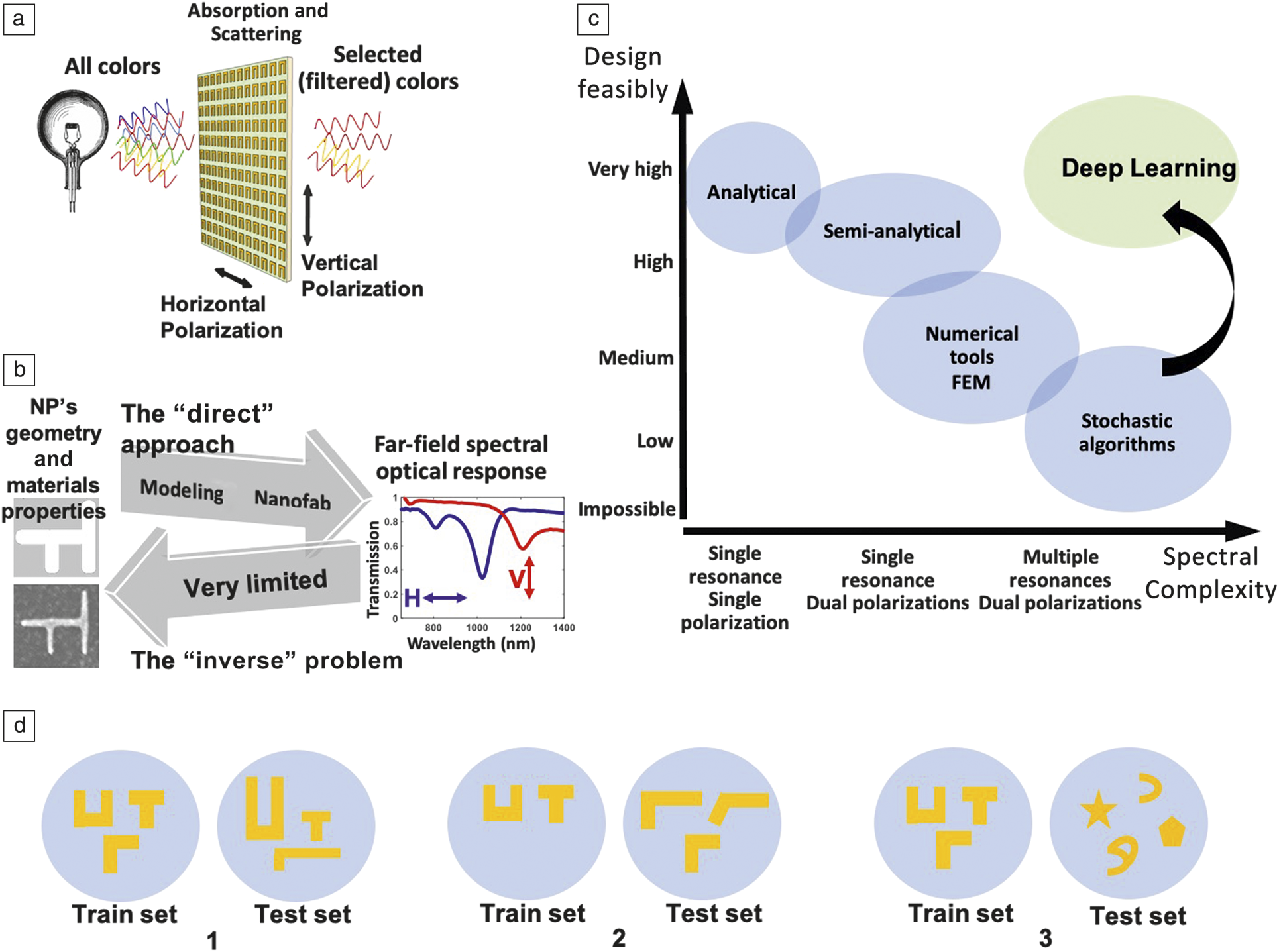
The major contributions to date that have been published to design nanostructures by utilizing machine learning techniques can be categorized into three categories (Figure 1d). The first, and the most fundamental one, is obtaining a model that is capable of designing nanostructures from the same shape and material it was trained on, but with different properties, such as sizes, angles, and host material. As we discuss in greater detail next, in works that fall within this category the general structure is maintained (particle with eight alternating shells or thin film with m alternating layers as presented in Figure 2 and Figure 3) and the machine learning algorithm works to provide optimized parameters of the structure.Reference Peurifoy, Shen, Jing, Yang, Cano-Renteria, DeLacy, Joannopoulos, Tegmark and Soljacˇic´1–Reference Ma, Cheng and Liu4 Our previous work, which introduced a model that was trained on different shapes, such as “H,” “h,” “n,” and “L” with given matched spectra, also falls within this category.Reference Malkiel, Mrejen, Nagler, Arieli, Wolf and Suchowski5
Design of thin-film multilayer filters for on-demand spectral response using neural networks.Reference Liu, Tan, Khoram and Yu2 (a) A thin film composed of m layers of SiO2 and Si3N4. The design parameters of the thin film are the thicknesses of the layers d i (i = 1, 2, ..., m), and the device response is the transmission spectrum. (b) The forward neural network takes D = [d 1, d 2, ..., d m] as inputs and discretized transmission spectrum R = [r 1, r 2, ..., r m] as output. A tandem network is composed of (left) an inverse design network connected to a (right, dashed box) forward modeling network. The forward modeling network is trained in advance. In the training process, weights in the pretrained forward modeling network are fixed and the weights in the inverse network are adjusted to reduce the cost (i.e., error between the predicted response and the target response). Outputs by the intermediate layer M (labeled in blue) are designs D. (c, d) Example test results for two different target designs queried with the tandem network method showing successful retrieval compared to the target design. Note: c, speed of light; a, maximum allowed thickness of each layer.

Multilayer shell nanoparticle inverse design using neural networks (NNs).Reference Peurifoy, Shen, Jing, Yang, Cano-Renteria, DeLacy, Joannopoulos, Tegmark and Soljacˇic´1 (a) The NN architecture has as its inputs the thickness (x i) of each shell of the nanoparticle and as its output the scattering cross section at different wavelengths of the scattering spectrum (y i). (b) NN versus numerical nonlinear optimization. The legend gives the dimensions of the particle, and the blue is the desired spectrum. The NN is seen to solve the inverse design much more accurately.

The second category incorporates models that are able to generalize and design geometries with shapes that differ from the set of shapes used during training, but are still considered to be in the same family (i.e., the model can generalize to other shapes that are similar, but not identical, to the set of shapes it was trained on). Attempts to devise such a model have recently been presented where the parameters of the model are the pixel of a two-dimensional (2D) image, allowing a more versatile and general representation of structures.Reference Liu, Zhu, Rodrigues, Lee and Cai6 The third category is a model that is able to design any geometry, with any shape, achieving what the deep learning community calls the generalization capability. The generalization ability of such models needs to be verified via a proper holdout test set (i.e., a test set) comprising structures sampled from a completely different distribution than the set the model was trained on. To this end, studies that provide a model that is able to design nanostructures for any spectra should exercise extra care in constructing a test set that would verify the generalization level of the model at hand.
The categories discussed above are ordered by the complexity of the learning task, where each category relates to a different level of robustness or generalization. The most desirable capability is the last category, which can design any geometry with any shape.
Under the context of the model at hand and the assumption that a large volume of data is available for learning, the first step to achieve such a generic capability is to design a model that has enough degrees of freedom to allow the design of any geometry.
In this article, we review the topic of inverse design in nanophotonics based on deep learning architectures and compare the advantages and weaknesses of the main published approaches. We also expand our current approach toward the goal of inverse design of any nanostructure with at-will spectral response.
Deep learning versus optimization and genetic algorithms
The deep learning approach to inverse design in nanophotonics is still in its infancy and needs to be evaluated against more established optimization techniques that have been presented over the years. We therefore start with a general comparison, along the lines presented in Table I, between the deep learning approach and genetic algorithms, the most widely used type of optimization algorithm, for the inverse design of nanophotonics devices.Reference Malkiel, Mrejen, Nagler, Arieli, Wolf and Suchowski5,Reference Malkiel, Nagler, Mrejen, Arieli, Wolf and Suchowski7,Reference Malkiel, Mrejen, Nagler, Arieli, Wolf and Suchowski8
Performance comparison with respect to different parameters between different computational approaches (shallow neural network, deep neural network, and genetic algorithms).

Note: AI, artificial intelligence; MSE, mean squared error.
A genetic algorithm is an optimization method inspired by natural selection. Such an algorithm can be used to solve optimization tasks by searching for a good solution among many possible solutions, with regard to a predefined set of constraints. This task is further defined by a fitness function that measures the quality of a candidate solution. The goal is to find a solution that maximizes the fit function subject to the constraints. In order to find a good solution, the algorithm, similar to natural selection, evolves generations of possible solutions. At the beginning of the process, the algorithm starts with a random set of simple solutions; it evaluates each one of them and then chooses which will be carried over to the next generation and how. Some possible solutions can move with no change to the next generation, some will be randomly mutated, and some will be randomly matched with other solutions, thus creating a new descendant candidate.
In each generation, all of the possible solutions are evaluated in order to search for the best fit, and the process terminates when a good solution is found or when a predefined threshold of the number of generations is reached. Although the nondeterministic search of the genetic algorithm could lead to the discovery of nontrivial solutions, genetic algorithms are not suitable for tasks where the computation of the fitness function is computationally demanding. The algorithm relies on evaluating every single possible candidate in every generation, so if the evaluation time is demanding, the process becomes intractable.
As a specific example, evaluating a single spectrum of a given three-dimensional (3D) geometry for a single polarization for that wavelength range takes at least one minute to several tens of minutes even when using efficient scattering calculations such as the discrete dipole approximation,Reference Draine and Flatau9 as there is no analytical solution for the scattering of a general 3D geometry. This practical, simple runtime constraint makes a genetic algorithm not relevant to this type of task since each generation is composed of hundreds or thousands of experiments that demand hours of computations for each generation and days for a single design task.
In comparison to evolutionary algorithms and other similar stochastic optimization methods, mainstream learning techniques such as deep learning optimize a generic model during the training process. Although there may be a relatively long training process, using such a network to predict new samples typically takes less than 1 s. In the approach developed by the authors,Reference Malkiel, Mrejen, Nagler, Arieli, Wolf and Suchowski5,Reference Malkiel, Nagler, Mrejen, Arieli, Wolf and Suchowski7 training the network takes up to 3 h. When the training process is complete, each query takes 3 ms to compute. This way, given a query, deep learning would design a solution in 3 ms, while a genetic algorithm will perform thousands of simulations where each one of the simulations could take hours to perform.
We emphasize that the evolutionary approach is fundamentally different since for every single design task, it searches the parameter space over dozens (sometimes hundreds) of generations with each generation encompassing dozens or hundreds of individual designs (e.g., individuals). For this reason, the individuals should be simple enough to analytically solve for their electromagnetic response, otherwise the optimization task will take a prohibitive amount of time and thus limit the usefulness of such an approach.
The deep neural network (DNN) approach is radically different. A DNN is trained on a set encompassing structures that are not trivial, for which the response must be calculated using time-consuming numerical approaches. However, once the data set is created and learned, this task is nonrecurring, and each design task takes only a query of the DNN, which takes only a few milliseconds.
Recent advances in DNNs for nanophotonics
In this section, we review recent advances in DNNs applied to the inverse design problem of nanophotonic devices. Recently, we introduced the bidirectional neural network for the design of nanostructures (Figure 4).Reference Malkiel, Mrejen, Nagler, Arieli, Wolf and Suchowski5,Reference Malkiel, Mrejen, Nagler, Arieli, Wolf and Suchowski8 The bidirectional model, which proceeds from the optical response spectrum to the nanoparticle geometry and then back, solves both the inverse problem of designing a nanostructure and the direct problem of inferring the optical characteristics of the designed geometry. The advantages of the bidirectional model are twofold. First, this model is able to streamline the design process by retrieving an immediate prediction for the optical properties of the designed nanostructure. In this model, the designer can match the desired spectra (as depicted in Figure 1a) with the recovered spectra, which can also be used in understanding the confidence level of the model for the specific design. Second, a bidirectional model allows co-adaptation between both directions, leading to better robustness and higher stability for the predictions.
Our previous workReference Malkiel, Mrejen, Nagler, Arieli, Wolf and Suchowski5,Reference Malkiel, Nagler, Mrejen, Arieli, Wolf and Suchowski7,Reference Malkiel, Mrejen, Nagler, Arieli, Wolf and Suchowski8 introduced a bilateral deep learning (DL) network able to predict the response (in two polarizations) of any of the structures defined in the “H” family (see main text). It also allows the design of “H” structures based on the required response. (a) The “H” geometry is parametrized to allow easy vector representation where the presence of Legs 1–5 is binarily coded (1 = leg present, 0 = leg absent). Note: L 1 = length of Legs 1, 2, 4, and 5; L 0 = Leg 3 length; φ = Leg 1 angle. (b) The network architecture allows the input of the horizontal and vertical spectrum vectors (sampled at 43 wavelength points each) as well as a material’s properties vector representation (43 parameters). This input is then fed into the first three fully connected 100 neuron (described by the solid black circles) layers followed by eight fully connected layers. The DL is given a (c) measured horizontal polarization (horizontal red double-headed arrow) and (d) vertical polarization (vertical blue double-headed arrow). (e) The predicted geometry, which is in good agreement compared to the geometry measured in scanning electron microscope (inset [c]). Comparison between the fed spectra and the predicted ones are found in (c, d). Note: DNN, deep neural network.

The model we introduced was trained on synthetic data centered around different variants of the H shape, and was also applied on measured spectra from nanofabricated materials from our laboratory. This model was the firstReference Malkiel, Nagler, Mrejen, Arieli, Wolf and Suchowski7 neural-based architecture applied for the design of a nanostructure, but its architecture is inherently limited to the H family (Figure 4). To date, this is the only experimental demonstration of geometry prediction capability of a deep learning network.
Ma and co-workers introduced a model for the design of chiral metamaterials incorporating two bidirectional networks along with a synthetic data set composed of a vectorized representation of geometries associated with materials, reflection spectra, and circular dichroism spectra.Reference Ma, Cheng and Liu4 The dual bidirectional model comprises two networks, a primary network and an auxiliary network. The primary network predicts the back and forth geometry encoding vector and its associated reflection spectra (Figure 5a). The auxiliary network predicts the back and forth geometry (represented as an encoding vector) and its associated circular dichroism spectra. Both networks are separately trained using the previously discussed data set. The authorsReference Ma, Cheng and Liu4 show that a model that combines both the auxiliary network and the primary network yields more accurate predictions.
Bidirectional deep learning network applied to the design of chiral metamaterials.Reference Ma, Cheng and Liu4 (a) Schematic of the designed chiral metamaterial. The inset is the zoomed-in structure of a single meta-atom. (b) A bidirectional deep neural network is designed to retrieve the chiral metamaterial geometry from the reflections (σ+-input-σ+-output [blue curve], σ–-input-σ–-output [green curve]), and the cross-polarization term σ+-input-σ–-output (red curve) and CD, and vice versa. (c, d) CD spectra predicted by the deep neural network (blue dots), which are in good agreement with the simulations (red curve). Note: CD, circular dichroism; σ+, σ– right-handed and left-handed circular polarization, respectively.

Sajedian and co-workers suggest a neural network that solves the direct problem of inferring spectra for a given geometry (Figure 6).Reference Sajedian, Kim and Rho3 This problem can be solved via (slow) simulations, and is considered to be more feasible compared to the ill-posed inverse problem of inferring a geometry for on-demand spectra.
Spectrum prediction for one polarization based on the geometry represented as a 2D map of pixels using convolutional neural networks. (a) Convolutional neural networks are used to extract spatial features from an image of a structure by extracting data from smaller parts of the image. (b) (Right) The solid blue lines show the absorption curves obtained from the simulation package (SIM) for (left) a random geometry, and the dotted orange lines show the absorption curves predicted by the deep learning (DL) model. These curves show a one-to-one comparison of predicted absorption value versus real absorption value for each frequency. Adapted with permission from Reference Sajedian, Kim and RhoReference 3. © 2019 Nature Publishing Group. Note: relu, rectified linear unit.

Liu and co-workers propose a generative adversarial network (GAN)—an algorithm that uses two neural networks that contest each other to generate new data—for generating 2D nanostructure images from spectra (Figure 7).Reference Liu, Zhu, Rodrigues, Lee and Cai6 The authors created a synthetic data set of geometries associated with multiple families, such as squares, circles, sectors, crosses, and shapes from the Modified National Institute of Standards and Technology (MNIST) data set (which incorporate handwritten digits [numbers]). The authors demonstrated the ability of the model to randomly design test samples from each one of the families previously discussed, using a model that was trained with samples from all families. This evaluation corresponds to Category 1 previously presented in Figure 1d, as the model task is to infer geometries from the same template it already saw in the training (this time, only with different attributes such as sizes and angles).
Generative adversarial networks-based inverse design of metasurfaces.Reference Liu, Zhu, Rodrigues, Lee and Cai6 (a) Three networks, the generator, the simulator, and the critic constitute the complete architecture. The generator accepts the spectra T and noise z and produces possible patterns. The simulator is a pretrained network that approximates the transmittance spectrum T̂ for a given pattern at its input, and the critic evaluates the distance of the distributions between the geometric data and the patterns from the generator. While training the generator, the produced patterns vary according to the feedback obtained from S and D. Valid patterns are documented during the training process, and are smoothed to qualify as candidate structures. (b) Test patterns are depicted in the top row and the corresponding generated patterns are listed in the bottom row. Each shape provides a sample of the different classes of geometric data input to the critic network. Note: S, simulator network; D, critic network.

During a second evaluation, Liu and co-workers tested a higher level of generalization, which correlates to the second category previously described.Reference Liu, Zhu, Rodrigues, Lee and Cai6 In this evaluation, the authors used a holdout test set composed of a complete subfamily set of geometries. Specifically, and to showcase the capability of their approach, the authors decided to keep all of the samples that correspond to digit “5” from the MNIST family in a holdout test set and trained their model on the rest of the data set. They reported the topologies of the predicted geometry and the original (i.e., ground truth) geometry differ considerably (the predicted geometry comprised a variation of the digit “3”), but the overall spectra of the predicted geometry possess similar features to the input spectra, with some discrepancies in a few specific locations.Reference Liu, Zhu, Rodrigues, Lee and Cai6
In addition, the authors argue that without GAN training, their model collapses and generates images of random pixels. When optimizing an inverse function of a single network, one can often obtain a solution that satisfies the inversion criteria; however, this does not create a valid input, as has been shown in the case of adversarial examples.Reference Goodfellow, Shlens and Szegedy10 This is why, similar to the mapping between MNIST and SVHN (the Street View House Numbers) digits results presented,Reference Taigman, Polyak and Wolf11 a GAN loss is needed. An alternative way for GANs to improve generalization may be to rely on activations from multiple layers of the direct network, as is done in the perceptual loss.Reference Johnson, Alahi and Fei-Fei12
As previously mentioned,Reference Malkiel, Mrejen, Nagler, Arieli, Wolf and Suchowski5,Reference Malkiel, Mrejen, Nagler, Arieli, Wolf and Suchowski8 we introduced a model able to infer geometries of the same or similar shapes it was trained on (Category 1), which have variable sizes, angles, and the permittivity (epsilon) of the host materials. However, in order to be able to design any geometry, one needs to allow for larger degrees of freedom. Specifically, our model architecture was designed to retrieve coding vectors that encode the geometry shape to the “H” family. To circumvent the inherent limitation of this encoding, further degrees of freedom were obtained as we asked the model to predict each edge presence, the length of the edge, and the angle between the inner edge and the top right edge.Reference Malkiel, Mrejen, Nagler, Arieli, Wolf and Suchowski5,Reference Malkiel, Nagler, Mrejen, Arieli, Wolf and Suchowski7,Reference Malkiel, Mrejen, Nagler, Arieli, Wolf and Suchowski8
Toward generalization
Recent work in computer vision has suggested pix2pix,Reference Isola, Zhu, Zhou and Efros13 a neural-based model that learns to map images from the source domain to the target domain. Given an input image, the model learns to generate images according to some ground truth image labels. Applied on different types of data sets, pix2pix showcases the ability of neural networks to generate realistic images that preserve different types of underlying logic, such as mapping gray images to color images, facade labels to images, maps to aerial views.
Following the pix2pix approach, and by building upon our previous work, we recently published the spectra2pix model,14 which aims to expand our capabilities to the second or even third more desirable categories. The model focuses on solving the inverse problem of inferring a nanostructure geometry from a given spectrum and material properties. Compared to the previous bidirectional model, the spectra2pix architecture supports the generation of any geometry by training the model to regress the raw pixel values of the 2D images of the geometries at hand. The training task is enforced by optimizing the spectra2pix model to minimize a pixelwise loss term, applied on the generated image with the ground truth image. In this new work, we published a new version of our data set, incorporating the 2D images of the geometries. The data set and the code can be found on Github.15
In spectra2pix, we utilize the data set from References 5 and 7. This data set comprises ∼13 K samples of synthetic experiments, where each sample is associated with a geometry, a single polarization (vertical or horizontal), and materials properties. By pairing the polarization, we formed ∼6 K experiments comprising the quadruplet of horizontal spectrum, vertical spectrum, epsilon host dielectric, and 2D image of the geometry. The epsilon host dielectric values vary in the range of 1.0 to 3.0.
The geometries are composed of different combinations of edges, which together form a template with the shape “H.” All three data parts, geometry, spectrum, and material properties are represented as vectors. Using spectra2pix, we were able to transform the previously discussed data set from the vectorized representation of the geometry encoding into 2D binary images comprising geometry shapes. A sample of the transformed images, along with the matched spectra of each geometry can be seen in Figure 8. The transformed data set is available for the public on Github.15
Six samples from the transform data set of spectra2pix.Reference Malkiel, Mrejen, Wolf and Suchowski14,Reference Malkiel15 We see the wide variety of (left) spectra and (right) geometries spanned by the family of the “H” shapes. The spectra correspond to horizontal and vertical polarizations in transmission. In all experiments, the structures are made of gold, each with a different host dielectric, with dielectric values varying in range (1.0, 3.0) (not shown in the figure). Each image is composed of 64 × 64 pixels, with a pixel size of 15.625 × 15.625 nm.

The architecture of spectra2pix is composed of two parts. The first part is built upon our previous work and utilizes three sequences of fully connected layers, each receiving a vectorized representation of a different part of the input data (two polarizations and host material). A few key properties of the second part of the architecture were adapted from pix2pix work, for which, following the fully connected sequences, the spectra2pix model reshapes the internal vectorized representation into a 2D matrix and utilizes a sequence of convolutional layers. The last layer in this model is a convolutional layer, with a single filter, which outputs a 2D image of the desired geometry.
To study the ability of spectra2pix to generalize, we split the previously discussed data set into train, test, and validation sets. The test set contains all of the geometries of the shape “L” and its variants. The train set contains all of the rest of the experiments (H family shapes), leaving 5% as a holdout validation set. The spectra2pix network was trained for 1 M training steps. We used the validation set for early stopping. At the end of the training, we used the model to infer geometries for the test set.
Figure 9 shows a representative sample from the test set predictions. Each row represents a different query. The left column (Figure 9a) displays the input spectra (both vertical and horizontal polarization), the middle (Figure 9b) presents the generated geometry, and the right (Figure 9c) showcases the ground truth label.
Results of queries with three designs from the test set (“L” family) to spectra2pix after the learning phase.Reference Malkiel, Mrejen, Wolf and Suchowski14 (a) Input spectra are presented; (b) the predicted geometry by spectra2pix, and (c) the ground truth geometry is depicted. Each image is composed of 64 × 64 pixels, with a pixel size of 15.625 × 15.625 nm.

These results indicate that the spectra2pix is fairly able to generate unseen geometries sampled from a different distribution than what the model was trained on.
Compared to the research reported in Reference 5, in the spectra2pix work, we utilize our model and showcase its ability to converge without GAN training, and more importantly, we demonstrate a successful generalization ability of the model to design a complete unseen subfamily set of geometries, taken from a somewhat different distribution the model was trained on. This generalization capability is associated with category two previously described.
Conclusions
The use of machine learning techniques, and deep learning in particular, has spawned huge interest over the past few years in the nanophotonics communities, due to the great promise these techniques offer for the inverse design of novel nanophotonic devices and functionalities. In this article, we have reviewed the main advances that have occurred in the past four years. We discussed the advantages and weaknesses of the different approaches presented so far, and introduced our spectra2pix network, a model composed of ultimate degrees of freedom, which conceptually allows the design of any 2D geometry. In addition, we presented the ability of spectra2pix to successfully generalize the set design of a completely unseen subfamily of geometries. Our results highlight the importance and the generalization ability of DNNs toward the goal of inverse design of any nanostructure with at-will spectral response.
Acknowledgments
Funding from the Israel Science Foundation under Grant No. 1433/15 is acknowledged. The contribution of I.M. is part of PhD thesis research conducted at Tel Aviv University.

Itzik Malkiel is a doctoral candidate in the School of Computer Science at Tel Aviv University, Israel, and a senior researcher on the Recommendation Machine Learning Research Team with Microsoft Corporation. He received his BSc degree in computer science from the Hebrew University, Jerusalem, in 2010. He received his MSc degree in computer science from Tel Aviv University, Israel, in 2016. Prior to joining Microsoft, he was a research scientist with GE Global Research and a senior software engineer and project leader. His current research focuses on machine learning (ML) and deep learning and includes topics such as medical imaging, computer vision, natural language processing, and ML applications in physics. Malkiel can be reached by email at itzik.malkiel@gmail.com.
Michael Mrejen is a research scientist in the Femto-Nano Laboratory in the Department of Condensed Matter Physics, School of Physics and Astronomy, at Tel Aviv University, Israel. He obtained his PhD degree in applied science and technology from the University of California, Berkeley, in 2015, and MSc degree in applied physics at Hebrew University, Jerusalem, in 2007. He received his BSc degree in optical engineering in 2003 from Technion–Israel Institute of Technology, Israel. His research focuses on exploring ultrafast light–matter interactions in plasmonic nanostructures, silicon photonics, and two-dimensional materials, as well as applying machine learning to nanophotonics. He has published 16 peer-reviewed articles and holds four patents. Mrejen can be reached by email at michael.mrejen@berkeley.edu.

Lior Wolf is a full professor in the School of Computer Science at Tel Aviv University, Israel, and a research scientist with Facebook AI Research. From 2003 to 2006, he conducted postdoctoral research at the Massachusetts Institute of Technology. In 2004, he received his PhD degree from the Hebrew University, Jerusalem. He is a European Research Council grantee. His awards include the International Conference on Computer Vision (ICCV) 2001 and ICCV 2019 honorable mention, and the best paper awards at the European Conference on Computer Vision 2000, the post-ICCV 2009 Workshop on eHeritage, the pre-Computer Vision and Pattern Recognition Workshop on Action Recognition, and the Internet Corporation for Assigned Names and Numbers 2016. His research focuses on computer vision and deep learning. Wolf can be reached by email at wolf@cs.tau.ac.il.

Haim Suchowski is an associate professor in the Department of Condensed Matter Physics, School of Physics and Astronomy, at Tel Aviv University, Israel. He received his BA degree in physics and BSc degree in electrical engineering, both in 2004, from Tel Aviv University, and his MSc degree in physics in 2006 and PhD degree in physics in 2011 from the Weizmann Institute of Science. His research focuses on exploring ultrafast dynamics in condensed-matter physics, nanophotonics, and two-dimensional materials. Suchowski also conducts research in nonlinear optics and in quantum coherent control with ultrashort laser pulses. He has 43 articles and 10 patents. He received the Fulbright Postdoctoral Fellowship and was recently awarded a European Research Council Grant for his project “MIRAGE 20-15.” Suchowski can be reached by email at haimsu@tauex.tau.ac.il.


 Open access