


Introduction
A basal zone of ice that interacts with the glacier bed is common to many glaciers and ice streams. This zone is typically debris-rich and has a low concentration of air bubbles relative to the sedimentary englacial ice, indicating its subglacial origin (bubble-free ice may be formed in other ways as well; e.g. Luthi and others, Reference Luthi, Fahnestock and Truffer2009). The basal zone also commonly possesses internal structures, such as banding or zonation at various scales, which frequently display folding, boudinage or other deformational features. Basal ice such as that observed at Matanuska Glacier is derived from subglacial waters – both glacial melt and surface-derived – which freezes and incorporates debris by processes of regelation or hydraulic supercooling (Alley and others, Reference Alley, Lawson, Evenson, Strasser and Larson1998). Within the basal zone, there is commonly a layer several meters thick that exhibits a banding – termed ‘stratification’ by Lawson (Reference Lawson1979a) – that arises from alternating layers of debris-poor and debris-rich ice (Fig. 1). The mechanism by which this stratification arises is poorly understood, and might either reflect pseudo-seasonal hydraulic fluctuations at the glacier bed or be a foliation resulting from post-freeze-on segregation and deformation within the basal zone (Alley and others, Reference Alley, Lawson, Evenson, Strasser and Larson1998). The origin of this stratification is of interest because of its implications for ice flow and processes of subglacial sediment entrainment and transport. Additionally, in situ melting of stratified basal ice contributes to the formation of melt-out till, a not-uncommon type of till that until recently has been both variably and poorly understood (Larson and others, Reference Larson, Menzies, Lawson, Evenson and Hopkins2016).
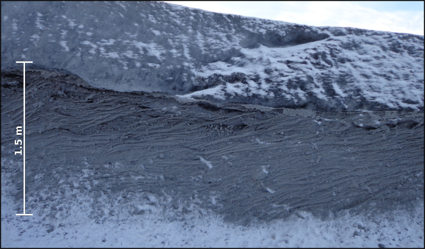
Basal ice exposure near our sample location (see Fig. 2). Photograph looking toward the SW. Note the abrupt transition from the clean englacial ice, above, to the debris-rich stratified ice, and the consistent up-glacier (to the left) dip of the debris-rich horizons.
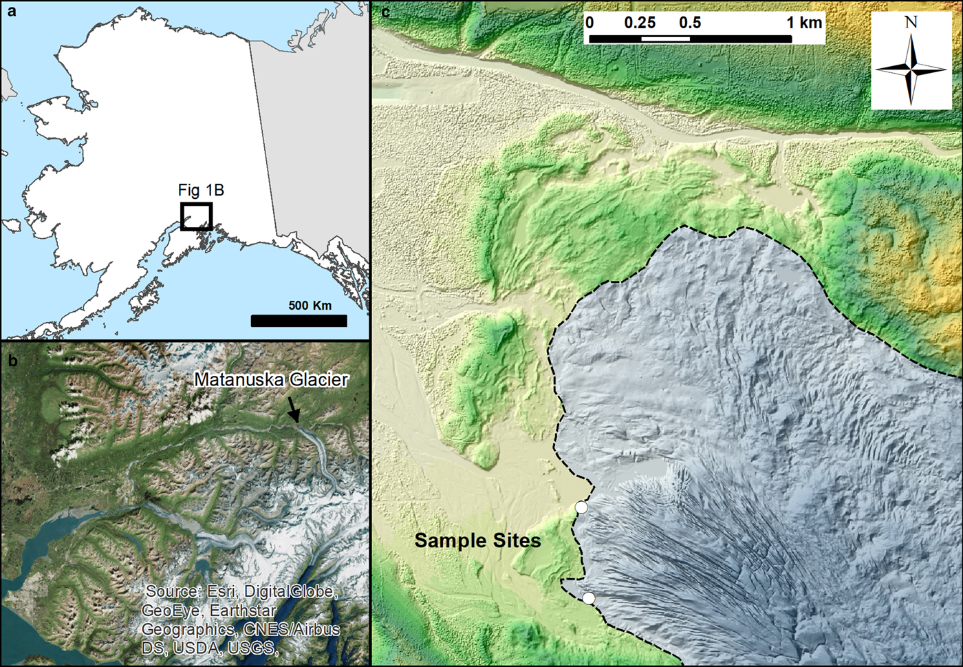
(a) Location map indicating the study area in southern Alaska. (b) Satellite image of the Chugach Range, Anchorage Lowland and the Matanuska Valley, including the prominent Matanuska Glacier. (c) LiDAR DEM and hillshade of Matanuska Glacier's terminus, including the primary sampling sites and ice margin (dashed line and shading).
Fabric – the preferred orientation of clasts, grains, particles and crystals – is a common tool used to learn about depositional and deformational processes. In glacial geology, ‘macrofabric’ refers to the orientation of macroscopic grains, commonly pebbles, and is an easy, low-cost way to investigate glacial processes. However, this tool is limited by grain size (i.e. application to fine-grained sediments requires special sample preparation and microscopic or other examination) and the potential for unintentional user bias (Chandler and Hubbard, Reference Chandler and Hubbard2008). Anisotropy of magnetic susceptibility (AMS) has a long history of application in structural geology as an indicator of relative strain in rocks (e.g. Borradaile, Reference Borradaile1988; Pares, Reference Pares2004; Ferre and others, Reference Ferre, Gebelin, Till, Sassier and Burmeister2014). AMS is dominantly controlled by the shape and distribution of magnetic grains (Tarling and Hrouda, Reference Tarling and Hrouda1993), and thus provides a robust, volume-averaged and objective alternative to traditional measurements of the fabric where environmental conditions and material properties are amenable to sampling and analysis.
In a novel investigation of the basal ice of Tunabreen, Svalbard, Fleming and others (Reference Fleming2013) demonstrated the potential of the AMS method for evaluating deformation kinematics in the basal zone of modern glaciers. After collecting samples using a drill designed for the recovery of cores for paleomagnetic analysis, Fleming and others measured the AMS of a total of 61 samples from six sites located across the exposed terminus of the glacier. The samples possessed a measurable AMS, dominated by the susceptibility of paramagnetic sediments. The diamagnetic susceptibility of ice contributed insignificantly to the AMS. The mean maximum AMS susceptibility axis paralleled ice flow direction, trending to the north (359°) with a 20° plunge. The maximum susceptibility axes were also found to parallel macroscopic deformation structures, such as sheath folding, elongated bubbles and stretching lineations. Additionally, the similarity of the fabric of basal ice to that of subglacially deformed materials led the authors to postulate that the March (Reference March1932) model of grain rotation may also apply to the deformation kinematics of basal ice. Overall, the AMS results of Fleming and others provide further evidence that non-coaxial strain plays a significant role in the deformation of basal ice.
Because the basal zone is composed of distinct facies of ice with differing morphologies and concentrations of debris, we expect AMS to be variable within the basal zone and, perhaps, to reflect rheological variations. Herein, we apply the AMS technique to the stratified basal ice of Matanuska Glacier, Alaska, USA, to evaluate the nature and distribution of strain within the basal zone. Specifically, we use a dense sampling of two exposures to (1) characterize the magnetic mineralogy of the basal zone of Matanuska Glacier; (2) characterize the AMS ellipsoid and fabric of debris-rich and debris-poor ice facies; (3) evaluate the influence of debris concentration on the fabric in the basal zone. Subsequently, we discuss the implications our results have on our understanding of the rheology of debris-ice mixtures contextualized by a thorough understanding of the grain-scale forces acting to align the particles within the basal ice.
Field setting
The Matanuska Glacier (Figs 2a, b), located ~150 km NE of Anchorage, AK, USA, is an ~48 km long temperate glacier, which drains NNW from the ice fields of the Chugach Mountains. The Matanuska is well-known for excellent exposures of stratified basal ice, and has a particularly well-developed stratification. The glacier has been remarkably stable throughout much of the Holocene (Williams and Ferrians, Reference Williams and Ferrians1961). The terminal lobe of the Matanuska (Fig. 2c) is ~4 km wide, the eastern portion of which is stagnant and covered with supraglacial debris; the western, debris-free portion is active and is the location of this study.
During winter months, ice advance causes the terminus of the glacier to thrust over morainal debris and stagnant buried ice, exposing the base of the glacier and providing access to the basal zone. This phenomenon provides excellent exposures of the englacial ice and some or all of the basal ice, sometimes extending into subglacial sediments. The basal zone of the Matanuska was first described in detail by Lawson (Reference Lawson1979a, Reference Lawson1979b). The Matanuska is a remarkably well-studied glacier, so the discussion that follows is largely a summary of the relevant details from Lawson (Reference Lawson1979a, Reference Lawson1979b, Reference Lawson1981), as well as additional relevant observations published in the literature.
The basal zone of the Matanuska ranges from 1 to 15 m thick when exposed; however, the thicker exposures are packages of ice stacked by low-angle thrusts. Basal ice has been observed, at one time or another, along the entire width of the active portion of the glacier, and has been detected geophysically and traced up-glacier ~300 m (Arcone and others, Reference Arcone, Lawson and Delaney1995; Lawson and others, Reference Lawson1998; Baker and others, Reference Baker2003). Lawson (Reference Lawson1979a, Reference Lawson1979b) provided detailed descriptions of the englacial and basal zones, and identified facies useful for characterizing the ice. The englacial ice – the debris-free or nearly-debris-free glacier ice constituting most of the glacier – can be subdivided into the diffuse and banded facies; however, the englacial zone is outside the scope of this work. The basal zone is characterized by three facies: dispersed, stratified and suspended. The dispersed facies is commonly found directly below the englacial ice, and the transition between the two is abrupt. This facies can be thin (~0.2 m) to thick (8 m), and in some localities non-existent. Debris within the dispersed facies is uniformly distributed and rarely clustered; debris typically represents 8% of the sample by mass.
The stratified and suspended facies (Fig. 1) underly the dispersed facies, and the contact is well-defined, but irregular. The most striking feature of the basal ice is the apparent stratification that arises from alternating layers of debris-poor and debris-rich ice. The debris-poor suspended facies is composed of fine-grained ice (typically <4 mm, Lawson, Reference Lawson1979c), and is generally bubble-free; when present, air bubbles are elongated in the direction of ice flow. Within these layers, debris is commonly present in irregularly shaped silt aggregates at grain intersections. The debris-rich stratified facies contains predominantly silt-to-coarse sand in well-defined semi-planar layers. In some cases, layers are ice-supported, and in others, ice is present only in the interstices between clasts. Clasts as large as cobbles are occasionally present, and are mostly subround and lack striations. Layers are generally semi-continuous at the scale of the exposure, and commonly dip up-glacier 10–15°. Debris layers are commonly 1–3 cm thick, and extend for several meters. See Larson and others (Reference Larson, Menzies, Lawson, Evenson and Hopkins2016) for a complete description of the sedimentology of the stratified basal ice.
The freeze-on process for the basal zone of the Matanuska has been identified as hydraulic supercooling of subglacial waters rising from an overdeepening near the glacier terminus (Alley and others, Reference Alley, Lawson, Evenson, Strasser and Larson1998). An overdeepening beneath the active portion of the glacier is readily identified by a zone of heavy crevassing immediately up-glacier of the modern glacier terminus, and has been characterized geophysically (Lawson and others, Reference Lawson1998; Baker and others, Reference Baker2003). In the summer months, frazil ice can be observed forming at vents near the glacier terminus (Lawson and others, Reference Lawson1998; Evenson and others, Reference Evenson1999). This frazil ice is produced as the pressure is released from supercooled water as it rises from the overdeepening, resulting in rapid ice crystal growth and entrainment of suspended and, in some cases, bedload sediments (Alley and others, Reference Alley, Lawson, Evenson, Strasser and Larson1998). Isotopic studies of the basal zone of the Matanuska indicate that rainfall runoff in addition to glacial melt is an important component of the basal waters, and that growth of the basal zone ice post-dates the production of bomb-produced tritium in the atmosphere (Lawson and Kulla, Reference Lawson and Kulla1978; Strasser and others, Reference Strasser, Lawson, Larson, Evenson and Alley1998; Titus and others, Reference Titus, Strasser, Lawson, Evenson and Alley1999).
Sampling and methodology
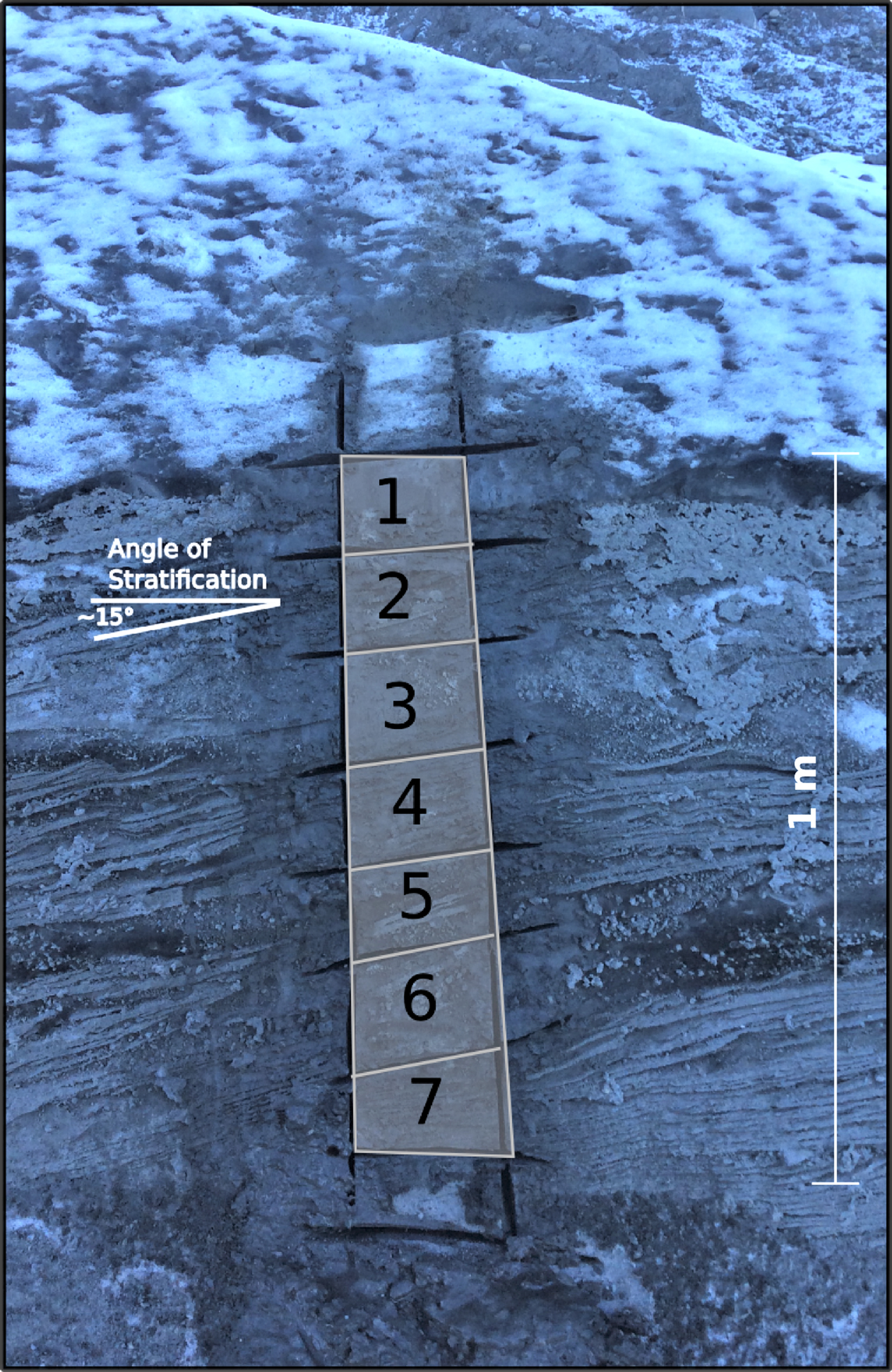
The basal zone of Matanuska Glacier was sampled in two locations on the western front of the active portion of the glacier. The northern sample site (Fig. 2) provided an ~1.5 m-thick section of the stratified basal ice underlying a thin (~4 cm) section of dispersed facies. Here, the layering within the stratified facies displays a relatively uniform up-glacier dip of ~15°. At the section sampled, the basal zone was capped by ~0.5 m of clean (debris-free), englacial ice. Samples were collected for AMS analysis and determination of debris content from one vertical column extending from the upper contact of the basal zone to the base of the exposure (Fig. 3). Additional samples were collected at the southern sample site (Fig. 2), which exhibited easily collectable distinct stratified and suspended facies; these samples were analyzed separately and will be referred to as the ‘facies samples’. At each site, large (15 cm × 15 cm × 10 cm) samples were cut using a concrete saw, oriented using a Brunton compass, and extracted from the exposure using a chisel and hammer. Orientation marks were carved into the samples, which were subsequently tightly sealed with plastic wrap and bagged to minimize sublimation during storage. Each sample collected was subsampled into ~8 cm3 specimens and inserted into standard paleomagnetic sample boxes. In total, 267 specimens were retrieved from the column in Figure 3 for analysis at Lehigh University. The facies specimens (117 total) were visually classified as stratified or suspended facies, according to the dominance of suspended silt aggregates or stratified layers, and shipped to the Institute for Rock Magnetism, University of Minnesota for analysis. To minimize melting, samples were kept in a cooler with dry ice between cuts and measurements.
Strategy for collecting seven specimens (numbered) from the uppermost 1 m of the ~1.5 m-thick section of basal ice. The snow-covered upper portion is debris-free englacial ice. Specimens were not collected from the cuts above specimen 1 or below specimen 7.
AMS was measured at Lehigh University using a KLY-3S Agico Kappabridge (Brno, Czech Republic) following the 15 static orientation scheme of Jelinek (Reference Jelinek1981). Additional specimens were measured at the Institute for Rock Magnetism, University of Minnesota, using an Agico MFK-1a susceptibility bridge with an automatic three-axis sample rotator. The orientation-dependent susceptibilities were fit using the least-squares method to an AMS ellipsoid defined by the maximum (k 1), intermediate (k 2) and minimum (k 3) susceptibility axes.
For this investigation, we will evaluate the AMS of basal ice in two ways. First we will evaluate the AMS ellipsoid of individual specimens using anisotropy (P’) and shape (T) factors (Hrouda, Reference Hrouda1982):


Subsequently, we will investigate the fabric, a higher-order orientation analysis of the AMS ellipsoids contained within a sample. In our study, each sample contains a minimum of 30 specimens. Therefore, each fabric is a composition of 30 or more ellipsoids. This distinction is important, as the information content of the AMS ellipsoids and the fabric to which they contribute are different.
Following convention within glacial geology, the fabric orientations are characterized using the eigenvalue method of Mark (Reference Mark1973), wherein a symmetric second-rank tensor is fit to the distribution of each susceptibility axis (e.g. k 1) and described by the principal eigenvector orientations (V 1, V 2 and V 3), and their associated eigenvalues (S 1, S 2, S 3, with S 1 + S 2 + S 3 = 1). V 1 is the orientation of maximum clustering, the degree of which is described by S 1, where S 1 = 0.33 indicates an isotropic distribution and S 1 = 1 indicates a perfectly aligned population of axes. In the fabric analysis of till, it is common to analyze the fabric using the k 1 orientation, which becomes oriented parallel to the shear direction and possesses a characteristic up-glacier plunge relative to the shear plane defined by the k 2 axis (e.g. Hooyer and others, Reference Hooyer, Iverson, Lagroix and Thomason2008; Iverson and others, Reference Iverson, Hooyer, Thomason, Graesch and Shumway2008). Since the attitude of the shear plane is rarely known independently, magnetic fabrics must be evaluated using all three axes to avoid significant misinterpretations (Iverson, Reference Iverson2017). To further define fabric shapes and the clustering of axes, we employ the metrics of Benn (Reference Benn1994) and plot the isotropy (I = S 3/S 1) and elongation (E = 1−S 2/S 1) for each susceptibility axis on a two-variable ternary diagram.
Results
Magnetic mineralogy
A series of magnetic experiments were conducted at the Institute for Rock Magnetism to determine the magnetic mineralogy of the basal ice. Leftover pieces of ice from cutting the cubic AMS samples were allowed to dry and the sediment was collected for measurement.
Low-temperature experiments were conducted on a Quantum Designs (San Diego, CA, USA) Magnetic Properties Measurement System. A specimen was cooled from 300 to 20 K in the presence of a 2.5 T field and the magnetic remanence (field cooling, remanence) was measured upon warming back to 300 K. Subsequently, the specimen was cooled to 20 K in the absence of a field, a low-temperature saturation isothermal remanent magnetization (SIRM) of 2.5 T was applied, and the remanence was measured upon warming to 300 K (zero field cooling, remanence). The specimen was then subjected to a room temperature SIRM of 2.5 T and the magnetic remanence was measured upon cooling and warming between 300 and 20 K. In all curves, the specimen goes through the ~120 K magnetite Verwey transition (Verwey, Reference Verwey1939) and the ~34 K pyrrhotite Besnus transition (Besnus, Reference Besnus1966), indicating that both magnetite and pyrrhotite are present (Fig. 4a).
(a) Low-temperature (de)magnetization data showing a pyrrhotite Besnus transition (T B) at ~34 K and a magnetite Verwey transition (T V) at ~120 K in the field-cooled (FC), zero field-cooled (ZFC) and room temperature saturation isothermal remanent (SIRM) magnetization curves. (b) High-temperature susceptibility. The heating (red) curve shows a peak in susceptibility preceding pyrrhotite's Curie temperature (Py) and a marked drop of susceptibility associated with magnetite's Curie temperature (Mgt). The cooling (blue) curve reveals an increase of susceptibility consistent with the production of magnetite upon heating. (c) Unmixing of backfield demagnetization data revealing two superimposed distributions of magnetic grains centered at coercivities of 15.7 and 41.6 mT, likely corresponding to magnetite and pyrrhotite (see text for details).
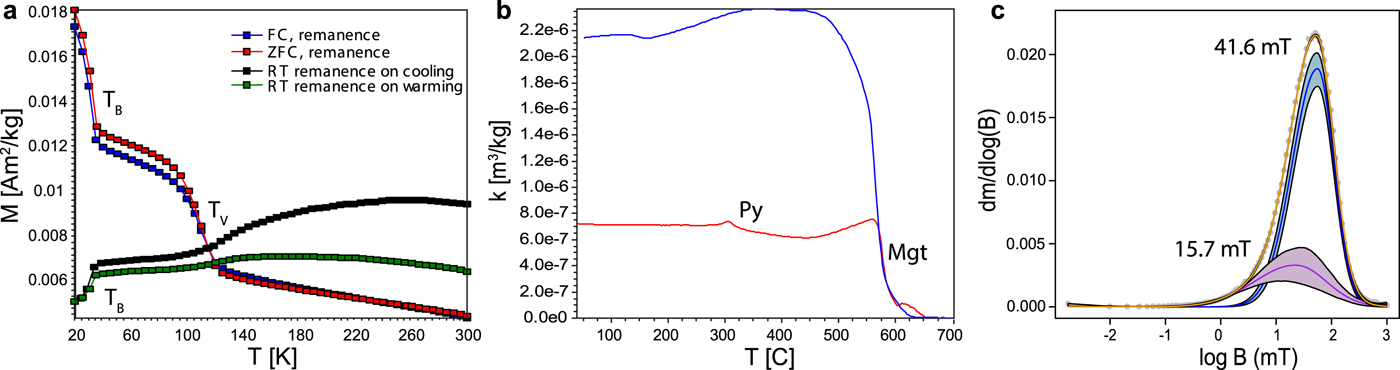
High-temperature susceptibility measurements were performed on a KLY-2 Agico (Brno, Czech Republic) susceptibility bridge. Heating curves reveal a small peak followed by a decrease of susceptibility at ~320°C consistent with the unblocking of pyrrhotite grains close to their Curie temperature (Dunlop and Özdemir, Reference Dunlop and Özdemir1997) (Fig. 4b). A second broader increase of susceptibility is observed starting ~500°C and is followed by a sharp drop at magnetite's Curie temperature (580°C). The increase of susceptibility is attributed to the creation of new magnetite upon heating, likely from clay minerals, as confirmed by the enhanced susceptibility upon cooling. A small fraction of susceptibility persists to ~650°C and is interpreted as the inversion of oxidized magnetite (maghemite) to hematite upon heating (Dunlop and Özdemir, Reference Dunlop and Özdemir1997).
Unmixing of a backfield demagnetization curve (Maxbauer and others, Reference Maxbauer, Feinberg and Fox2016) reveals that two dominant populations of magnetic grains are present and can be fitted with two overlapping distributions centered at ~15.7 and 41.6 mT (Fig. 4c). The unmixing of backfield curves provides non-unique solutions, as evidenced by the uncertainty envelopes around the fitted components; however, the mean coercivities are consistent with a distribution of magnetite and pyrrhotite grains within the PSD grain size range.
These rock-magnetic data are mutually consistent, and demonstrate that the AMS of these glacial sediments is carried by a mixture of magnetite and pyrrhotite. Furthermore, the PSD grain size suggests the maximum and minimum principal susceptibility axes of these grains coincide with the long and short axes of the grains, indicating that these grains record normal susceptibility fabrics (e.g. Jackson, Reference Jackson1991). The data suggest that paramagnetic grains are also present, likely phyllosilicates and clay minerals, which may contribute to the AMS. However, their contribution is likely small in the presence of ferrimagnetic magnetite and pyrrhotite.
Ice facies AMS characterization
Debris content
Average debris content of the facies specimens is 38.4 ± 18.8% by weight (wt.%); individual specimens range from 1.2 to 67.1 wt.%. The debris contents within the stratified and suspended facies are 52.0 ± 9.74 and 23.9 ± 14.9 wt.%, respectively. These values are consistent with the previous observations at Matanuska Glacier (Lawson, Reference Lawson1979).
AMS parameters
AMS ellipsoids of the facies samples (Fig. 5a) vary considerably in both degree of anisotropy (P’) and shape (T). This is representative of the total population of samples, as has been observed in previous AMS investigations (e.g. Gentoso and others, Reference Gentoso2012; Fleming and others, Reference Fleming2013; Hopkins and others, Reference Hopkins, Evenson, Kodama and Kozlowski2016). Taken as a whole, T values indicate dominantly triaxial to oblate (positive) fabrics, but range from nearly perfectly prolate (−0.89) to nearly perfectly oblate (0.9). Variation of T is also large (mean std dev. of 0.4). P’ shows significantly less variability. When samples are classified according to facies (Fig. 5b), anisotropy of the stratified facies is less variable (P’ = 1.05 ± 0.04) and the shape is consistently oblate (T = 0.46 ± 0.37). The AMS of the suspended facies is dominantly triaxial with P’ values similar to, and sometimes much higher than, the stratified facies.
Bivariate plot of specimen-level AMS anisotropy (P’) and shape (T) factors for specimens classified as suspended and stratified facies (a) and facies mean anisotropies with 1-sigma error bars (b).
AMS fabric
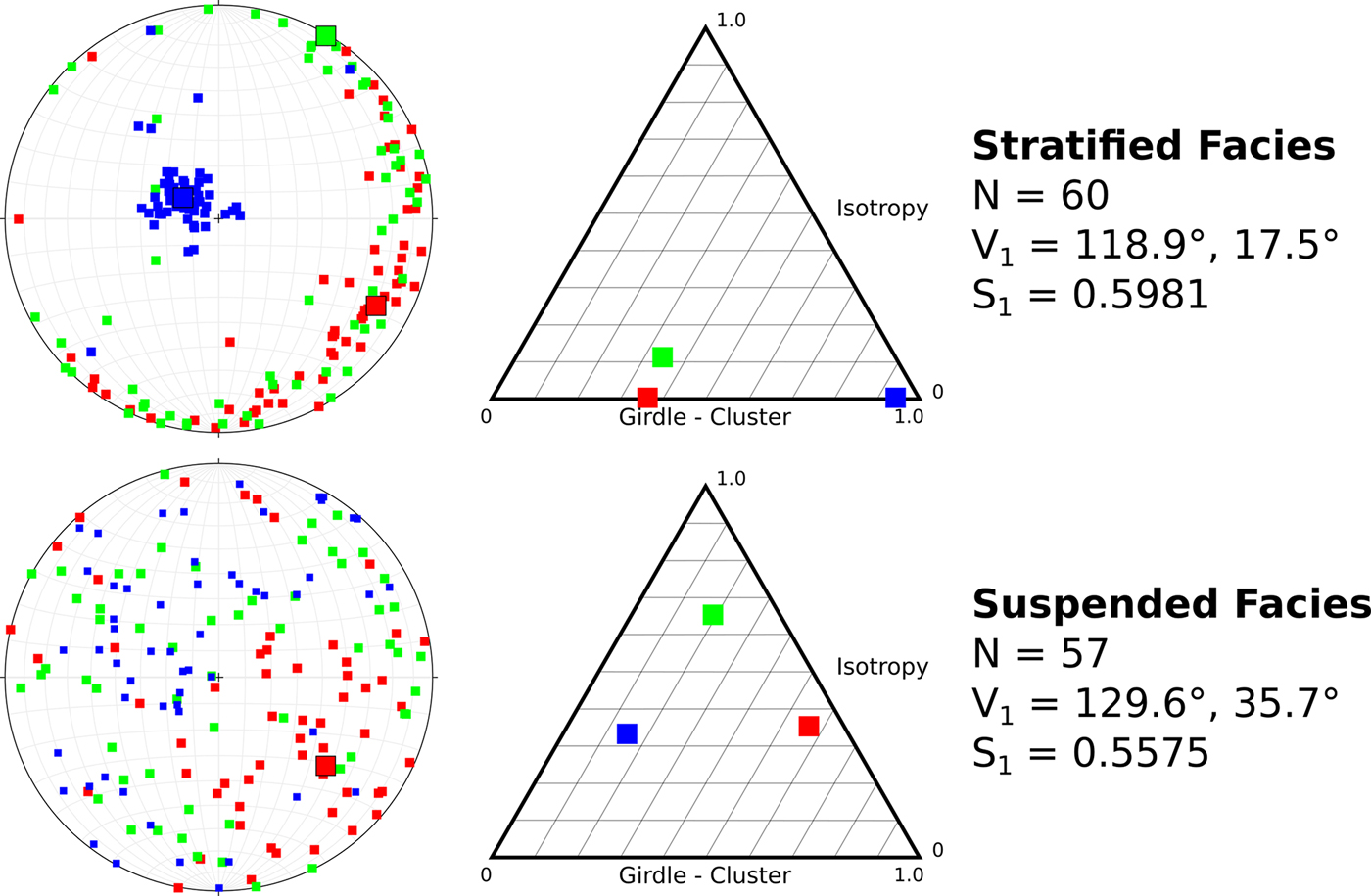
The characteristic AMS fabric of each facies is markedly different (Fig. 6). The stratified facies possesses a well-developed, girdled fabric with a V 1 parallel to ice flow and plunging up-glacier 17.5° within the plane of the stratification. Intermediate axes concentrate near horizontal, and the minimum axes are tightly clustered perpendicular to the k 1–k 2 plane. In contrast, the suspended facies possesses a nearly isotropic fabric.
Stereographic projections in a geographic coordinate system (left) and ternary shape diagrams (center) of AMS fabrics for basal ice facies. Individual AMS k 1 (red), k 2 (green) and k 3 (blue) axes are displayed using small squares; V 1 axes are presented using large squares for axes with E > 0.5.
Fabric: vertical distribution
AMS fabrics for each sample from Figure 3 are presented in Figure 7. Sample 1, the uppermost fabric spanning the englacial, dispersed and stratified facies of ice, possesses a near random fabric for all the susceptibility axes. This specimen is also characterized by low debris content (17 ± 18 wt.%). All lower samples are exclusively within the stratified facies of ice, and possess anisotropic fabrics (Fig. 7). Specimens 2, 4, 5 and 7 display significant clustering of their k 1 axes (S 1 > 0.6, E > 0.5), and the V 1 trends for these fabrics are parallel or sub-parallel to the known ice flow direction (NW). These samples generally display insignificant plunge (⩽5°) down-glacier, except for the lower-most fabric (sample 7). Sample 7 possesses the strongest fabric of this section (S 1 = 0.8565), and plunges 16° up-glacier.
AMS fabrics for each sample. Fabrics are presented in lower-hemisphere stereographic projections in a geographic coordinate system, with north toward the top of the page. Ice flow is to the NW. Individual AMS k 1 (red), k 2 (green) and k 3 (blue) axes are displayed using small squares; V 1 axes are presented using large squares for axes with E > 0.5. Column 2 (from left) presents k 1 orientations with 2-sigma Kamb contours. Column 3 presents k 1 rose diagrams. k 1 fabric statistics and V 1 trend and plunge are shown in column 4. Two-variable (E, I) ternary shape diagrams are presented in column 5. Specimen sample descriptions and dominant facies are shown in column 6.

Fabric shape parameters, characterized using the ternary plots of Benn (Reference Benn1994), are shown in column 5 of Figure 7 and Table 1. Three of the four fabrics discussed above possess significant clustering around all three axes, with specimens 4 and 6 being the exception. The two specimens discussed above (3, 6) whose k 1 axes do not parallel ice flow display girdle fabrics within the k 1–k 2 plane. All fabrics within the stratified facies possess significant clustering around the k 3 axis, and in all cases this axis is near-vertical.
Sample debris content (weight %), fabric strengths (S 1) and fabric shape characteristics (I & E)

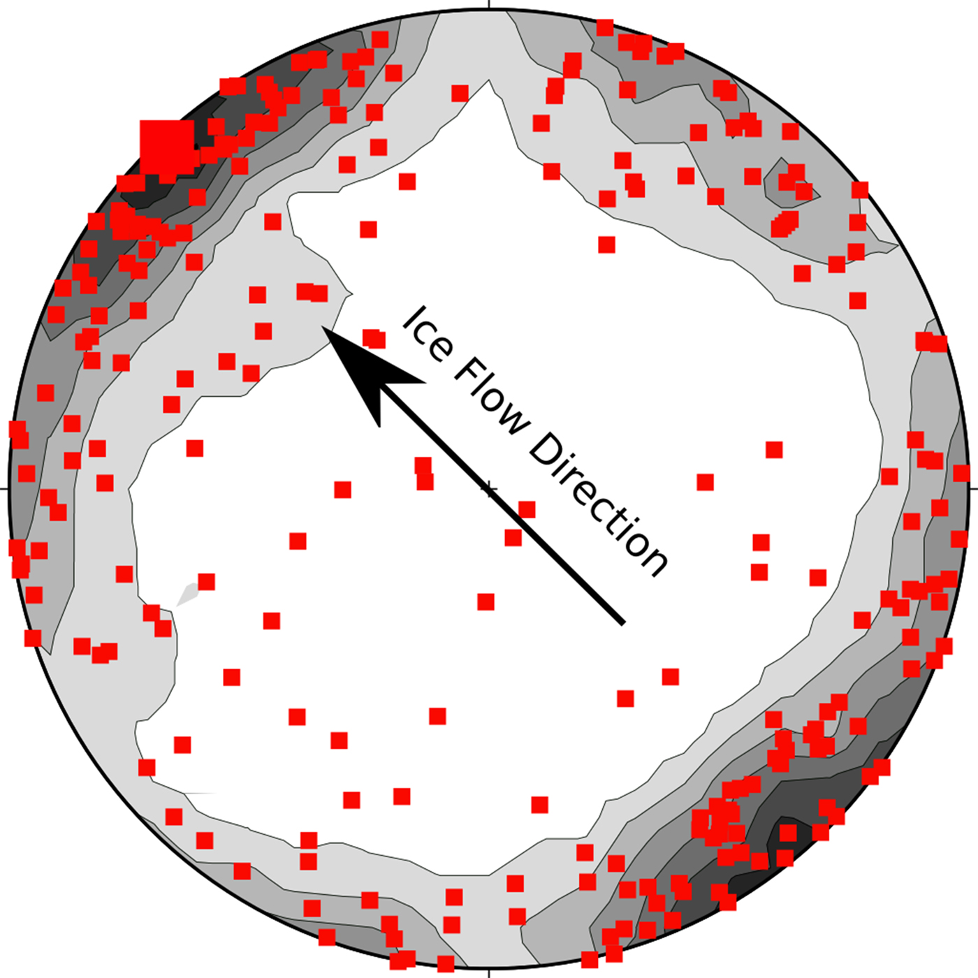
The bulk k 1 fabric of all specimens (Fig. 8) in this section parallels ice flow (V 1 = 316°, 2°), but displays weak clustering (S 1 = 0.5506). Fabric shape (I = 0.213; E = 0.403) indicates that the k 1 axes are weakly girdled in the horizontal plane, which is to be expected from averaging the clustered, girdled and isotropic fabrics displayed above. The girdle is better described as a bimodal distribution, with one cluster parallel to ice flow (315°) and another oriented perpendicular to flow, possibly representing an intersection lineation or switching of the k 1 and k 2 principle axes. The perpendicular k 1 orientations are largely sourced from samples 3 and 6, and possess anisotropy ellipsoids otherwise typical of the larger measured population.
Stereographic projection of all specimen AMS k 1 orientations (small squares) from the northern sample site contoured using 2-sigma Kamb contours, mean V 1 (large red square) and ice flow direction are also shown.
Relationships between fabric parameters and debris content
Figure 9 explores the relationship between key descriptive measures of fabric and debris content. Consistent with the similar S 1 values for each facies, the strength of the fabric defined by the k 1 axes increases only slightly with increasing debris (Fig. 9a). Strength of the k 3 axis fabric shows a greater increase. Fabric elongation increases with increasing debris, while fabric isotropy decreases (Figs 9b, c). This relationship is significantly more pronounced for the k 3 axes, as would be expected for fabrics with k 1 and k 2 axes girdled within the shear plane.
Bivariate plots of fabric strength as measured by S 1 (a), fabric shape characteristics (E, I) for k 1 fabrics (b) and fabric shape characteristics (E, I) for k 3 fabrics (c).

Discussion
Fleming and others (Reference Fleming2013) found that AMS aligns with the deformation inferred from the structures observed in basal ice of a surge-type glacier, supporting the use of magnetic properties as a proxy for deformational history (see ‘Introduction’ section). We provide a brief review here of some of the physical processes controlling the orientation of magnetic particles (inclusions) in ice, finding broad support for Fleming and others (Reference Fleming2013), but with some nuance. Subsequently, we offer two potential explanations of the observed AMS of the basal ice of Matanuska Glacier.
Within a crystal at stresses and temperatures typical of glaciers, ice deforms almost entirely by dislocation glide on basal planes, but with no crystallographically preferred glide direction in those basal planes (see, e.g. Jacka and Budd, Reference Jacka and Budd1989; Cuffey and Paterson, Reference Cuffey and Paterson2010; Alley, Reference Alley1992 for reviews). Because polycrystalline glacier ice rarely if ever is deposited with its basal planes oriented for easy glide in the stress state of the glacier, this restriction of glide to basal planes causes incompatible deformation between neighboring grains, which is accommodated by grain rotation, grain-boundary sliding, and diffusion and deformation focused in the regions of potential overlap or gaps between neighboring grains. Additional grain-boundary sliding may also occur, contributing to the bulk deformation (Goldsby and Kohlstedt, Reference Goldsby and Kohlstedt2001).
The grain rotation associated with incompatible deformation of adjacent grains leads to the evolution of lattice-preferred orientations, with c-axes (the normal to the basal planes) rotating toward compressive axes in the large-scale stress field under ‘pure’ shear and rotating toward the normal to the shear plane under simple shear. This has the effect of making the ice harder for additional pure shear deformation, by reducing the resolved shear stress on basal planes, but making the ice softer in simple shear by aligning the shear planes of individual crystals with the shear plane of the glacier. Grain deformation also causes elongation of grains, and thus elongation and preferred orientation of grain boundaries.
This evolution of the grain-boundary structure and of c-axis fabric is opposed by additional processes, including subdivision of grains by strengthening of subgrain boundaries formed by interactions among dislocations, and by nucleation and growth of new, strain-free grains, which generally occurs with c-axes at high angles to stress axes such that there is a large resolved shear stress on the basal planes of the new grains. Under some conditions, a steady state may be reached in which nucleation and growth of new grains balance the deformation of old grains, producing a constant average grain size, grain shape, c-axis fabric, etc. Under other conditions, these characteristics continue to evolve with deformation.
Broadly, the net effect of simple-shear deformation of polycrystalline ice is to rotate grains such that their basal planes parallel the shearing direction, generally with some tendency to develop preferred orientation of grain boundaries also parallel to the shearing direction, and with adjacent grains experiencing similar deformation. Under pure shear, ice evolves toward basal planes in a ‘hard’ orientation, and during this evolution, adjacent grains deform in somewhat different ways. Under high stresses, nucleation and growth of new, strain-free grains occur with basal planes oriented at high angles to the applied stresses. In pure shear, this softens the ice but maintains incompatible deformation in adjacent grains. Some uncertainty remains about the onset, if any, of such nucleation-and-growth recrystallization in simple shear (Jacka and Budd, Reference Jacka and Budd1989). Such recrystallization is suppressed by high impurity or particulate concentrations that tend to slow or stop the migration of grain boundaries. Glaciers thus often contain relatively impure ice with a strong c-axis clustering that is deforming rapidly in simple shear, adjacent to ‘cleaner’ ice with a c-axis girdle or other relatively dispersed fabric.
Studies of the c-axis fabric and grain size of Matanuska Glacier are severely hampered by the difficulty of cutting thin sections through the ice with such high debris concentrations without causing localized melting (e.g. Ensminger and others, Reference Ensminger, Alley, Evenson, Lawson and Larson2001). Observations of sublimated surfaces in winter confirm expectations that the higher debris concentrations of the stratified facies are associated with finer-grained ice than in the suspended facies. Modern techniques such as electron backscatter diffraction might be applied in future targeted studies, but at present we lack c-axis data on the ice studied. Analogy to other settings suggests that the fine-grained high-debris-concentration stratified-facies ice has c-axes clustered toward the normal to the layering, and that the coarser-grained lower-debris-concentration suspended-facies ice has either a similar fabric or a multi-maximum girdle centered on the normal to the layering (e.g. Samyn and others, Reference Samyn, Svensson and Fitzsimons2008).
Non-spherical inclusions in the ice are rotated by flow, and spherical but deformable inclusions (e.g. bubbles) are deformed and then rotated. Inclusion orientations then can be used to interpret strain at the grain scale (Fegyveresi and others, Reference Fegyveresi, Alley, Voigt, Fitzpatrick and Wilen2018), as reviewed briefly here.
The magnetic inclusions in Matanuska Glacier basal ice likely include combinations of more-or-less prolate magnetic ellipsoids of ferrimagnetic magnetite and pyrrhotite and more-or-less oblate ellipsoids of paramagnetic phyllosilicates. In temperate ice such as the Matanuska Glacier, these mineral inclusions are likely separated from the ice by meltwater, producing a free-slip boundary. Sufficient cooling would increase coupling between ice and inclusions, but persistent pseudo-liquid layers would likely allow continuing slip for temperatures within a few degrees of the bulk melting point, with great cooling required to fully couple ice and inclusions (Dash and others, Reference Dash, Rempel and Wettlaufer2006). For a free-slip boundary, pure shear in ice will tend to orient prolate inclusions in the elongation direction, and oblate inclusions with their short axis in the direction of greatest compression; simple shear will orient prolate inclusions in the shear direction and oblate inclusions in the shear plane (e.g. March, Reference March1932; Ghosh and Ramberg, Reference Ghosh and Ramberg1976; Ildefonse and Mancktelow, Reference Ildefonse and Mancktelow1993). A no-slip boundary may allow an inclusion to rotate through the shear plane in simple shear, but with the slowest rotation near the shear plane, weakening the strength of fabric developed but not eliminating it, and maintaining the same relation to the stress state.
For any inclusion contained fully within a single ice crystal, this indicates that the direction of maximum elongation will rotate to align with the shear direction in the basal plane, with the minimum elongation normal to the shear plane. For a large inclusion crossing a grain (crystal) boundary, the situation may be somewhat complex, with influence from shear within both grains and from shearing in the grain boundary; however, the strong discontinuity in the grain boundary seems likely to dominate, so the inclusion would tend to be oriented with maximum elongation in the shear direction and minimum elongation normal to the grain boundary.
Triaxial (i.e. k 1 > k 2 > k 3) to girdle magnetic fabrics oriented sub-parallel to ice flow direction consistent with simple shear along a sub-horizontal shear plane dominate the basal ice of the Matanuska Glacier. This observation is also consistent with macrofabrics described in the basal zone of the Matanuska Glacier (Lawson, Reference Lawson1979; Hart, Reference Hart1995), and is in general agreement with the AMS fabrics of Fleming and others (Reference Fleming2013). Macrofabrics of the Matanuska are commonly moderately strong and plunge up-glacier, commonly within the plane of the stratification (Lawson, Reference Lawson1979), as would be expected under simple shear and as is commonly observed in subglacial tills. Up-glacier plunge is also observed in the magnetic fabrics of Fleming and others (Reference Fleming2013). The same relationship is observed here. Simple shear within the basal zone has been suggested previously for other glaciers based upon macroscopic structures, including folds, boudinage, pressure shadows and rotational clasts (Hubbard and Sharp, Reference Hubbard and Sharp1989; Hart, Reference Hart1998). These features are rarely observed at the Matanuska Glacier.
Magnetic anisotropy at the specimen-level is similar in debris-rich and debris-poor Matanuska Glacier ice (Fig. 5); however, averaging over multiple specimens produces isotropic to weakly developed magnetic fabrics in debris-poor ice, while debris-rich ice fabrics are well-developed with the k 1–k 2 axes girdled within the plane of stratification. Based on these magnetic fabrics, AMS indicates higher strain within debris-rich stratified facies ice but much less strain within debris-poor ice, or else the effects of recrystallization of ice crystals opposing the effects of strain on the magnetic fabric. The magnitude of strain indicated within debris-rich layers is perhaps variable; however, in most cases, it is significant. Fabric strengths reported here are comparable to AMS fabric strengths of deforming till beds (Shumway and Iverson, Reference Shumway and Iverson2009; Gentoso and others, Reference Gentoso2012; Vreeland and others, Reference Vreeland, Iverson, Graesch and Hooyer2015; Hopkins and others, Reference Hopkins, Evenson, Kodama and Kozlowski2016); however, given the expected significant differences in the deformation style of basal ice and till, direct comparisons should be avoided. We suggest, as did Fleming and others (Reference Fleming2013), that further work focusing on experimentally sheared debris-ice mixtures is needed.
There is no apparent trend in fabric strength throughout the ~1.5 m column sampled in this study. This is perhaps surprising (cf. Hart, Reference Hart1995), because the progressive growth of basal ice on the bottom of the glacier means that the uppermost samples are older than deeper ice. Several explanations are possible, and more than one mechanism may have contributed. Because the basal ice is thicker than the sampled interval (see ‘Field setting’ section), we have not characterized the full range of behavior, and there may be a trend that we lack the sensitivity to detect. Time evolution of basal strain rate during accretion as the ice flowed out of the overdeepening, coupled with depth variation of strain rate within the accreted ice from depth variation in stresses, could enhance or cancel depth variation in cumulative strain. We note again that while samples presented in Figure 7 were classified according to dominant facies, individual specimens were not; thus, the strength of fabrics in Figure 7 may not be directly comparable or a reliable indicator of relative strain, because each fabric is likely a composite of both stratified and suspended ice facies.
The rheology of basal ice is significant for glacial dynamics, including subglacial sediment transport and vertical deformation profiles (e.g. Cuffey and others, Reference Cuffey, Thorsteinsson and Waddington2000). However, several mechanisms are involved, acting at rates affected by several factors (Hubbard and Sharp, Reference Hubbard and Sharp1989; Benn and Evans, Reference Benn and Evans2014; Moore, Reference Moore2014), such that adding debris to ice may either harden or soften it for further deformation (Ting and others, Reference Ting, Martin and Ladd1983; Moore, 2014). Significant factors include debris content, ice crystal size, ice fabric and the presence of unfrozen water.
While field evidence indicates that increasing debris content typically weakens ice and allows for increased and more rapid deformation (Brugman, Reference Brugman1983; Fisher and Koerner, Reference Fisher and Koerner1986; Echelmeyer and Zhongxiang, Reference Echelmeyer and Zhongxiang1987; Cohen, Reference Cohen2000), laboratory studies often indicate an apparent ‘hardening’ of ice associated with increasing debris concentrations (e.g. Hooke and others, Reference Hooke, Dahlin and Kauper1972; Baker and Bergerich, Reference Baker and Bergerich1979; Nickling and Bennet, Reference Nickling and Bennet1984). This discrepancy reflects the competing relationships between the variables mentioned above. Crystal size impacts ice strength, such that fine-grained ice tends to deform more readily, with grain size inversely related to debris content (Baker, Reference Baker1978; Baker and Bergerich, Reference Baker and Bergerich1979; Cuffey and others, Reference Cuffey, Thorsteinsson and Waddington2000). Therefore, increasing debris content may cause progressively smaller ice crystals, which in turn shifts more of the debris into grain boundaries or their intersection such that ice in debris-rich layers can be largely interstitial. Microstructures identified within the debris-rich basal zone of the Taylor Glacier suggest the importance of unfrozen water, which may allow slip across interfacial water films (Samyn and others, Reference Samyn, Fitzsimons and Lorrain2005, Reference Samyn, Fitzsimons and Lorrain2009). Thus, we consider it highly likely that deformation is concentrated in the debris-rich layers of the stratified basal ice as a result of decreased ice grain size and greater availability of unfrozen water associated with high debris and, presumably, solute content, and that the facies-dependent fabrics (Fig. 8) support that conclusion.
It is also possible that a scale-dependent bias contributes to our results. In the suspended facies, debris is concentrated into mm-scale clots at the intersections of coarse-grained ice. Within a representative 8 cm3 specimen, only a few clots are present. Sample anisotropy (P’, Fig. 5) is comparable to that of the stratified facies or even slightly stronger, indicating alignment within the clots, which may reflect some combination of cumulative strain and surface-tension effects. However, the orientation of the anisotropy may not align with the bulk shear direction because of local grain-scale deviations in stress and strain rate, which are expected under many circumstances, as described above. Averaging over many specimens then would yield the weak fabric observed in the suspended facies. In the finer-grained stratified facies with its greater debris concentration, local deviations of deformation from the bulk strain field are more fully sampled within a small volume, yielding weak specimen anisotropy but strong fabric. Based on our data and the results from other sites, we consider it likely that both mechanisms contribute: deformation is localized in the finer-grained layers with higher debris concentration, and the sampling scale of the AMS influences the results.
Conclusions
AMS fabric analysis within stratified basal ice of Matanuska Glacier supports the occurrence of simple shear within the basal zone, as expected physically and as observed for many other glaciers and ice streams. At the centimeter scale of individual AMS specimens, significant anisotropy occurs in both finer-grained ice with higher debris concentration and coarser-grained ice with sparser debris localized in clots. The finer-grained ice shows a stronger AMS fabric indicating more-consistent orientation of deformation in adjacent samples, likely both because of higher strain in the finer-grained ice, and because averaging over more grains in a single sample of finer-grained ice more completely removes the effects of local grain-scale deviations of deformation from the large-scale average. Simple shear parallel to ice flow appears to dominate. Future work is needed that further addresses the influence of debris concentration and other basal conditions on the behavior of basal ice and its potential influence on the flow and sedimentary dynamics of Matanuska Glacier and other glaciers.
Acknowledgements
This work benefited tremendously from helpful suggestions, discussion and hard work of Daniel Lawson, Grahame Larson, Josh Stachnik and Tom Pasquini. Additional thanks to Tom Pasquini and ExxonMobil for partially funding this research. Endless thanks to Bill and Kelly Stevenson for their graciousness in providing lodging, logistical support and entertainment. This article is IRM publication number 1813.


 Open access